Queues with Small Advice

Abstract

Motivated by recent work on scheduling with predicted job sizes, we consider the performance of scheduling algorithms with minimal advice, namely a single bit. Besides demonstrating the power of very limited advice, such schemes are quite natural. In the prediction setting, one bit of advice can be used to model a simple prediction as to whether a job is “large” or “small”; that is, whether a job is above or below a given threshold. Further, one-bit advice schemes can correspond to mechanisms that tell whether to put a job at the front or the back for the queue, a limitation which may be useful in many implementation settings. Finally, queues with a single bit of advice have a simple enough state that they can be analyzed in the limiting mean-field analysis framework for the power of two choices. Our work follows in the path of recent work by showing that even small amounts of even possibly inaccurate information can greatly improve scheduling performance.

1 Introduction

1.1 Motivation

In queueing settings where the required service time for a job is known, strategies that take advantage of that information, such as Shortest Job First (SJF) or Shortest Remaining Processing Time (SRPT) can yield significant performance improvements over blind strategies such as First In First Out (FIFO). However, exact knowledge of the service times is a great deal to ask for in practice. Here we consider the setting where one is given much more limited information. Specifically, we consider the case where, for each job, a queue gets only one bit of information, or advice, regarding the job size.

While a one bit limitation may seem unusual, there are both theoretical and practical motivations for such a study. Online algorithms with small amounts of optimal advice has been a subject of study in the theoretical literature (see, e.g., the survey [3]); such work highlights the potential for additional information to improve performance. Considering the case of just one bit of information is an interesting limiting case. Further, one-bit advice can naturally correspond to informing whether a job should be placed at the front or the back of the queue; for some queue implementations, such as in hardware or other highly constrained settings, one may desire this simplicity over more complicated data structures for managing job placement in the queue.

However, as a more concrete practical motivation, recently researchers have studied queues with predicted service times, rather than exact service times, where such predictions might naturally be provided by a machine learning algorithm [4, 13, 14, 15, 17, 19]. Indeed, the queueing setting is one natural example of an expanding line of work where predictions can be used to improve algorithms, particularly in scheduling (e.g., [8, 9, 11, 15, 17]). Our setting here of one-bit predictions can model a natural setting where the prediction corresponds to whether a job’s service time is believed to be above or below a fixed threshold. Such predictions may be simpler to implement or more accurate than schemes that attempt to provide a prediction of the exact service time.

For single-queue settings, our work uses standard queueing theoretic analysis techniques. Here we generally follow the (folklore) approach of using Kleinrock’s Conservation Law to derive formulae for the conditional waiting time of a job according to its service time; this approach dates back to at least the work of O’Donovan [16], from whose framework and notation we borrow. The derivations can also be readily obtained using the analysis of priority systems, following the framework presented in for example [6]. The goal here is not to suggest new methods of analysis, but instead:

• show how the problem of scheduling with limited predicted information can naturally be analyzed;

• demonstrate how even limited advice and predictions can provide large performance gains; and

• show some interesting derivations for the special case we refer to as exponential predictions.

We also examine one-bit predictions schemes with large numbers of queues using the power of two choices. Here each arrival chooses the better of two randomly selected queues (or more generally from $d$ randomly selected queues) from a large system of (homogenous) queues. This study shares many of the same motivations as for single queues; moreover, it may offer a first step to some open questions in the area, such as analyzing the power of two choices when using Shortest Remaining Processing Time or related schemes (see e.g. [14]).

Finally, more generally, we believe this work also highlights some aspects of using machine learning predictions that may provide guidance for the design of machine learning prediction settings. For example, we see that some predictions may be much more important than others; in queueing settings, it seems generally much more important to identify long jobs correctly than short jobs, as long jobs will block many other jobs from service.

2 Single Queues and One-Bit Threshold Schemes

2.1 Notation and Model

We consider M/G/1 queueing systems, with arrival rate $\lambda$ and where the processing times are independently sampled according to the cumulative distribution $F(x)$ with corresponding density $f(x)$. We follow some of the notation from [16]. We assume the expected service time has been scaled so the mean service time is 1 (that is, ${\bf E}[F]=1$). Note ${\bf E}[F^{2}]$ is the second moment for the service time. We further let

$$V =\frac{\lambda{\bf E}[F^{2}]}{2}$$

be the expected remaining service time of the job being served at the time of a random arrival. We also let

$$\rho(t) =\lambda\int_{0}^{t}xf(x)dx$$

be the rate at which load is added to the queue from jobs with service time at most $t$, and correspondingly

$$\rho(t) =\lambda\int_{\infty}^{t}xf(x)dx=\lambda.$$

2.2 The Conservation Law

As described in [16], Kleinrock’s Conservation Law says that for a queue with Poisson arrivals satisfying basic assumptions (such as the queue is busy whenever there are jobs in the system), the expected load $L$ on the system at a random time point (e.g., in the stationary distribution), satisfies

$$L(1-\rho) =V,$$

where again $V$ is the expected load due to the job in service and $\rho$ is the total rate at which load is added to the system. The law allows simple derivations of conditional expected waiting times, by looking at appropriate subsystems of jobs.

2.3 Analysis of One-Bit Threshold Schemes

We consider the case of an advisor that provides a single bit of advice per job. Specifically we consider the strategy where the advice bit is 0 if the job’s service time is less than some threshold $T$, and 1 otherwise. The job is placed at the front of the queue if the advice bit is 0, and at the back of the queue otherwise. We consider preemptive and non-preemptive queues, where in the preemptive case a job placed at the front will preempt the job currently receiving service. We later generalize the one bit of advice to prediction-based systems, where the prediction is whether the service time for the job is larger or smaller than the threshold.

2.4 The non-preemptive system

We first consider jobs arriving jobs with service time at most $T$. Here we do not require the conservation rule; such a job is placed at the front of the queue, although it has to wait for the job, if any, in service to complete. Further, any additional jobs of service time at most $T$ that arrive before this job starts service is placed ahead of the arriving job being considered. We denote the expected waiting time for a job with service time $t$, by which we mean the time spent by an incoming job in the stationary distribution waiting before starting to obtain service, by $W_{1}(t)$. We denote the expected sojourn time, by which we mean the entire time spent by an incoming job in the system, by $S_{1}(t)$.

The expected time an arriving job has to wait for an existing job being processed is $V$. It follows from standard busy period analysis that additional incoming jobs increase the expected waiting time by a factor of $\rho(T)$, and so

$$W_{1}(t) =\frac{V}{1-\rho(T)}.$$

The expected sojourn time for such jobs is thus

$$S_{1}(t) =\frac{V}{1-\rho(T)}+t.$$

For jobs with service time $t$ larger than $T$, we consider the subsystem of all jobs, and use the notation $W_{2}(t)$ and $S_{2}(t)$ for the corresponding quantities. In this setting we have

$$L =\frac{V}{1-\rho}$$

from the conservation law. For any job with service time larger than $T$, any new job with service time at most $T$ that arrives will be placed ahead of of this job until it is served. Hence

$$W_{2}(t) =\frac{L}{1-\rho(T)}$$

$$=\frac{V}{(1-\rho)(1-\rho(T))},$$

and

$$S_{2}(t) =\frac{V}{(1-\rho)(1-\rho(T))}+t.$$

For a given service distribution $F$ and threshold $T$, we have the total expected waiting time $W$ in the system is

$$W =\frac{VF(T)}{1-\rho(T)}+\frac{V(1-F(T))}{(1-\rho)(1-\rho(T))}$$

$$=\frac{V(1-F(T)\rho)}{(1-\rho)(1-\rho(T))}.$$

The expected sojourn time $S$ satisfies $S=W+1$. Minimizing $W$ (or $S$) can be accomplished numerically.

As an example we discuss through this work, for exponentially distributed service times, $V=\lambda$, $F(T)=1-e^{-T}$, $\rho=\lambda$, and $\rho(T)=(\lambda)(1-(T+1)e^{-T})$. We find the expected sojourn time for this case, which we refer to as $S_{e,n}$, is then

$$S_{e,n} =\frac{\lambda(1-\lambda+\lambda e^{-T})}{(1-\lambda)(1-(\lambda(1-(T+1)e^{-T})))}+1$$

$$=\frac{1-\lambda+\lambda(T+1)e^{-T}-\lambda^{2}Te^{-T}}{(1-\lambda)(1-(\lambda(1-(T+1)e^{-T})))}+1.$$

Taking the derivative, we find the optimal $T$ value occurs when

$$\frac{1}{\lambda}-1 =\frac{e^{-T}}{T-1},$$

or equivalently we seek $T$ that satisfies

$$\lambda =\frac{T-1}{e^{-T}+T-1},$$

In particular, as $\lambda$ goes to $1$, the optimal $T$ increases to infinity, and as $\lambda$ goes to 0, the optimal $T$ goes to 1. It is perhaps worth noting that a threshold $T$ of 4 corresponds to a $\lambda$ larger than $0.99$; that is, in this case, we do not see very large thresholds even under high load.

As another example, we consider service distributions following the Weibull distribution with cumulative distribution $F(x)=1-e^{-\sqrt{2x}}$. The Weibull distribution is heavy-tailed; while the average service time of this distribution remains 1, the second moment is 6, so there are many more very long jobs as compared to the exponential distribution. Weibull distributions are commonly used for queueing simulations, as heavy-tailed service time distributions are more realistic for many scenarios.

For this Weibull distribution, $V=3\lambda$ and $\rho(T)=\lambda(1-e^{-\sqrt{2T}}(T+\sqrt{2T}+1))$ are computed easily. The expected sojourn time in this case, which we denote by $S_{w,n}$, is then given by

$$S_{w,n} =\frac{3\lambda(1-\lambda+\lambda e^{-\sqrt{2T}})}{(1-\lambda)(1-(\lambda(1-e^{-\sqrt{2T}}(T+\sqrt{2T}+1))))}+1.$$

2.5 The preemptive system

We first consider jobs arriving jobs with service time at most $T$. Again, here we do not require the conservation rule; such a job is placed at the front of the queue, and any additional job of service time at most $T$ that arrive before this job starts service is placed ahead of the arriving job being considered. We use $W_{1}(t)$ and $S_{1}(t)$ as before.

Clearly $W_{1}(t)=0$. However, we also consider the effect of preemptions. Since any job of size at most $T$ will preempt the job, the expected sojourn time is

$$S_{1}(t) =\frac{t}{1-\rho(T)}.$$

For jobs with service times larger than $T$, we consider the subsystem of all jobs, and again use the notation $W_{2}(t)$ and $S_{2}(t)$ for the corresponding quantities.

In this setting we have

$$L =\frac{V}{1-\rho}$$

from the conservation law. While waiting any job of service time at most $T$ is placed ahead of any job of size greater than $T$, so again

$$W_{2}(t) =\frac{L}{1-\rho(T)}$$

$$=\frac{V}{(1-\rho)(1-\rho(T))}.$$

Because of the preemption, the expected time from the start of service until finishing service increases to $t/(1-\rho(T))$, and so

$$S_{2}(t) =\frac{V}{(1-\rho)(1-\rho(T))}+\frac{t}{1-\rho(T)}.$$

In this case the total expected waiting time is

$$W =\frac{V(1-F(T))}{(1-\rho)(1-\rho(T))},$$

and the total expected sojourn time is

$$S =\frac{V(1-F(T))+1-\rho}{(1-\rho)(1-\rho(T))}.$$

For exponentially distributed service times, we find the expected sojourn time in this case, which we refer to as $S_{e,p}$ is then

$$S_{e,p} =\frac{1-\lambda+\lambda e^{-T}}{(1-\lambda)(1-(\lambda(1-(T+1)e^{-T})))}.$$

One can readily that $S_{e,p}<S_{e,n}$ for any value of $T$; indeed,

$$\lambda S_{e,p} =S_{e,n}-1,$$

so

$$S_{e,n}-S_{e,p} =1-(1-\lambda)S_{e,p}>0.$$

Also, the optimal value of $T$ is again given by

$$\frac{1}{\lambda}-1 =\frac{e^{-T}}{T-1}.$$

For the Weibull distribution, we have the corresponding expression

$$S_{w,p} =\frac{1-\lambda+3\lambda e^{-\sqrt{2T}}}{(1-\lambda)(1-(\lambda(1-e^{-\sqrt{2T}}(T+\sqrt{2T}+1))))}.$$

3 Adding Predictions

We consider a simple model where the probability of a misprediction for a given item depends only on its service time, independent of other jobs and other considerations. Specifically, we suppose we have a desired threshold $T$, and our prediction is simply our best guess as to whether a job’s service time is larger or less than $T$. We define $g_{T}(x)$ be the probability that a job of size $x$ is predicted to be less than $T$. While one can imagine more complex prediction models, this model is quite natural, and is useful for examining the potential power of predictions.

3.1 The non-preemptive system

To deal with the predictions, we now let

$$Q(T) =\int_{0}^{\infty}f(x)g_{T}(x)dx,$$

and

$$\rho^{\prime}(T) =\lambda\int_{0}^{\infty}xf(x)g_{T}(x)dx.$$

Here $\rho^{\prime}(T)$ can be interpreted as the rate load arrives to the system from jobs with predicted service time at most $T$, and similarly $Q(T)$ is the fraction of jobbs predicted to have service time at most $T$.

We first consider arriving jobs with predicted service time at most $T$ and actual service time $t$. Following the same reasoning we have previously used, the waiting time ${W^{\prime}}_{t}$ for such jobs is given by

$${W^{\prime}}_{1}(t) =\frac{V}{1-\rho^{\prime}(T)}.$$

For jobs with predicted service time greater than $T$,

$${W^{\prime}}_{2}(t) =\frac{V}{(1-\rho)(1-\rho^{\prime}(T))}.$$

The total expected waiting time per job is therfore given by

$$W^{\prime} =\frac{V\int_{0}^{\infty}f(x)g_{T}(x)dx}{1-\rho^{\prime}(T)}+\frac{V\int_{0}^{\infty}f(x)(1-g_{T}(x))dx}{(1-\rho)(1-\rho^{\prime}(T))}$$

$$=\frac{V(1-\rho\int_{0}^{\infty}f(x)g_{T}(x)dx)}{(1-\rho)(1-\rho^{\prime}(T))}$$

$$=\frac{V(1-\rho Q(T))}{(1-\rho)(1-\rho^{\prime}(T))}.$$

In particular, we see that the only changes from the setting without the prediction is that in the $1-F(T)\rho$ term in the numerator, the $F(T)$ has been replaced by the more complex integral expression $Q(T)$, and similarly the $1-\rho(T)$ term in the denominator has become $1-\rho^{\prime}(T)$.

A model suggested in [13, 14] considers the setting where a prediction for a job with service time $z$ is itself exponentially distributed with mean $z$; we refer to this as the exponential prediction model. While not necessarily realistic, this model often allows for mathematical derivations, and provides a useful starting point for considering the effects of predictions. With this model,

$$g_{T}(x) =1-e^{-(T/x)},$$

and hence

$$Q(T) =\int_{0}^{\infty}f(x)g_{T}(x)dx$$

$$=1-\int_{0}^{\infty}e^{-x-(T/x)}dx$$

$$=1-2\sqrt{T}K_{1}(2\sqrt{T}),$$

where $K_{1}$ is a modified Bessel function of the second kind. Also

$$\rho^{\prime}(T) =\lambda\int_{0}^{\infty}(xe^{-x}-xe^{-x-(T/x)})dx$$

$$=\lambda(1-2TK_{2}(2\sqrt{T})),$$

where $K_{2}$ is a modified Bessel function of the second kind (with a different parameter).

The expected sojourn time for this case, which we refer to as $S_{e^{*},n}$, is then

$$S_{e^{*},n} =\frac{\lambda(1-\lambda(1-2\sqrt{T}K_{1}(2\sqrt{T})))}{(1-\lambda)(1-\lambda(1-2TK_{2}(2\sqrt{T})))}+1.$$

There does not appear to be a simple form for the derivative of this expression that allows us to write a simple form for the optimal value fo $T$, although it can be found numerically.

We can perform similar calculations for our Weibull distribution. Here we have

$$Q(T) =1-\int_{0}^{\infty}\frac{1}{sqrt2x}e^{-\sqrt{2x}-(T/x)}dx$$

$$=1-\sqrt{\frac{T}{2\pi}}G_{0,3}^{3,0}\left(\frac{T}{2}~{}|~{}-\frac{1}{2},0,\frac{1}{2}\right),$$

where here $G$ is the Meijer $G$-function.

Similarly

$$\rho^{\prime}(T) =\lambda\int_{0}^{\infty}\sqrt{\frac{x}{2}}\left(e^{-\sqrt{2x}}-e^{-\sqrt{2x}-(T/x)}\right)dx$$

$$=\lambda\left(1-\sqrt{\frac{T^{3}}{2\pi}}G_{0,3}^{3,0}\left(\frac{T}{2}~{}|~{}-\frac{3}{2},0,\frac{1}{2}\right)\right),$$

where again $G$ is the Meijer $G$-function.

The expected sojourn time for this case, which we refer to as $S_{w^{*},n}$, is then

$$S_{w^{*},n} =\frac{3\lambda\left(1-\lambda\left(1-\sqrt{\frac{T}{2\pi}}G_{0,3}^{3,0}\left(\frac{T}{2}~{}|~{}-\frac{1}{2},0,\frac{1}{2}\right)\right)\right)}{(1-\lambda)\left(1-\lambda\left(1-\sqrt{\frac{T^{3}}{2\pi}}G_{0,3}^{3,0}\left(\frac{T}{2}~{}|~{}-\frac{3}{2},0,\frac{1}{2}\right)\right)\right)}+1.$$

3.2 The preemptive system

For the preemptive system, again let

$$Q(T) =\int_{0}^{\infty}f(x)g_{T}(x)dx,$$

and

$$\rho^{\prime}(T) =\lambda\int_{0}^{\infty}xf(x)g_{T}(x)dx.$$

We first consider jobs arriving jobs with predicted service time at most $T$ and actual service time $t$ Such jobs will have no waiting time, but their expected sojourn time is

$$S_{1}(t) =\frac{t}{1-\rho^{\prime}(T)}.$$

For jobs with predicted service time greater than or equal to $T$, following the same reasoning as in the case without predictions, we have

$$W_{2}(t) =\frac{V}{(1-\rho)(1-\rho^{\prime}(T))},$$

and

$$S_{2}(t) =\frac{V}{(1-\rho)(1-\rho^{\prime}(T))}+\frac{t}{1-\rho^{\prime}(T)}.$$

We therefore find the total expected waiting time is

$$W =\frac{V(1-Q(T))}{(1-\rho)(1-\rho^{\prime}(T))},$$

and the total expected sojourn time is

$$S =\frac{V(1-Q(T))}{(1-\rho)(1-\rho^{\prime}(T))}+\frac{1}{1-\rho^{\prime}(T)}$$

$$=\frac{V(1-Q(T))+1-\rho}{(1-\rho)(1-\rho^{\prime}(T))}.$$

For the exponential prediction model, the expected sojourn time, which we refer to as $S_{e^{*},n}$, is then

$$S_{e^{*},p} =\frac{\lambda 2\sqrt{T}K_{1}(2\sqrt{T})+1-\lambda}{(1-\lambda)(1-\lambda(1-2TK_{2}(2\sqrt{T})))}.$$

We again here have the relation

$$\lambda S^{*}_{e,p} =S^{*}_{e,n}-1,$$

showing that preemption is always helpful in this setting.

For the Weibull model,

$$S_{w^{*},p} =\frac{1-\lambda+3\lambda\sqrt{\frac{T}{2\pi}}G_{0,3}^{3,0}\left(\frac{T}{2}~{}|~{}-\frac{1}{2},0,\frac{1}{2}\right)}{(1-\lambda)\left(1-\lambda\left(1-\sqrt{\frac{T^{3}}{2\pi}}G_{0,3}^{3,0}\left(\frac{T}{2}~{}|~{}-\frac{3}{2},0,\frac{1}{2}\right)\right)\right)}.$$

4 One-Bit Advice with Multiple Queues

In this section, we consider one-bit threshold schemes for setting with multiple queues. In particular, we consider the “power of $d$ choices” (also known as the “balanced allocations”) setting, where we consider the number of queues growing to infinity, and each arrival chooses the best queue from a small constant-sized subset of randomly selected queues [2, 12, 18]. An advantage here of queues based on one bit of advice is their state can easily represented, allowing the type of mean-field analysis that is typical for such systems. We note that analysis of the power of $d$ choices with for example exact job sizes using queueing schemes such as Shortest Remaining Processing Time remains an intriguing open question (see e.g. [14] for more discussion), although simply using FIFO queues and choosing the least loaded queue from a constant number of choices has been analyzed [7].

As our purpose here is primarily to demonstrate how schemes utilizing one bit can be analyzed in this framework, we choose a relatively simple example, based on the anecdotal 80-20 rule, that 20% of the jobs cause 80% of the work. We assume that there are two types of jobs: long jobs have exponentially distributed service times with mean $\mu_{1}$, and short jobs have exponentially distributed service times with mean $\mu_{2}<\mu_{1}$. Long jobs arrive with rate $\lambda_{1}n$ and short jobs arrive with rate $\lambda_{2}n$, where $n$ is the number of queues in the system. While this model is general, it can encompass the 80-20 rule, where long jobs are less frequent but require much more work; for example, if $\lambda_{1}\mu_{1}=4\lambda_{2}\mu_{2}$, then long jobs are relatively rare but contribute 80% of the work.

In the prediction setting, we assume long jobs are misclassified as short jobs independently with probability $q_{1}$, and short jobs are misclassified as long jobs independently with probability $q_{2}$. (We may view the case without predictions, where the one bit of advice is accurate, as corresponding to $q_{1}=q_{2}=0$, with the resulting equations.) A more useful interpretation for our analysis is that a job that is classified as a long job, or labeled long, is actually long with probability $p_{L}=\lambda_{1}(1-q_{1})/(\lambda_{1}(1-q_{1})+\lambda_{2}q_{2})$, and similarly a job that is classified as a short job, or labeled short, is actually short with probability $p_{S}=\lambda_{2}(1-q_{2})/(\lambda_{2}(1-q_{2})+\lambda_{1}q_{1})$. Similarly, the arrival rate for jobs that labeled long is $\lambda_{L}=\lambda_{1}(1-q_{1})+\lambda_{2}q_{2}$ and the arrival rate for jobs that are labeled short is $\lambda_{S}=\lambda_{2}(1-q_{2})+\lambda_{1}q_{1}$.

For serving jobs, we give labeled short jobs priority, and serve them in FIFO fashion; similarly, labeled longs jobs are served using FIFO. We suggest a simple, convenient method for choosing queues, although many variations are possible and can be studied similarly. We choose the “best” of $d$ queues chosen independently and uniformly at random for a constant $d$, where we determine the best as follows. First, an empty queue has highest priority; an empty queue will always be selected if it is one of the $d$ chosen. Otherwise, we ignore the label and the time already spent being served of the job being served. Jobs that are predicted to be short shall choose the queue with the fewest queued labeled short jobs, breaking ties in favor of the queue with the fewest labeled long jobs (and then randomly if two queues match), and similarly jobs that are predicted to be long shall choose the queue with the smallest number of queued labeled long jobs, breaking ties in favor of the queue with fewer short jobs (and then randomly if two queues match). Again, one could imagine more complex policies based on minimizing the expected time until service; such policies can be studied using the same framework.

We derive equations describing the system state in the mean field limit, where the number of queues goes to infinity. (This approach can be formalized using the theory of density dependent jump Markov chains, following the work of Kurtz; see [5, 10, 20] for examples.) The state of a single queue can be represented by a triple $(s,\ell,c)$, where $s$ is the number of jobs that are labeled short, $\ell$ is the number of jobs that are labeled long, and $c$ is 1 if the current running job is long and 2 if it is short. The state $(0,0,0)$ is used for an empty queue; this is the only state where $c\neq 1,2$. Let $x_{(s,\ell,c)}(t)$ represent the fraction of queues in state $(s,\ell,c)$ at time $t$; we drop the $t$ where the meaning is clear. We use ${\hat{x}}{(s,\ell,c)}$ to refer to the equilibrium values for these quantities.

Note that our setting allows a relatively simple analysis by having service times be exponentially distributed and predictions depend only on the type of the job, instead of its running time. Because of this, to keep the state of a queue it suffices to keep the type of the running job, as this gives the distribution of the remaining time it is in service. This approach can be extended to more general service times and predictions; see e.g. [1, 7], for example, for the appropriate framework. At a high level, for such generalizations, the state of the queue must track how long the current running job has been in the system; the distributions function for remaining time in service, which is derived by taking the proper weighted average over types, then determines whether the service will complete over the next time interval $dt$.

To write the equations describing the limiting behavior of these systems, we use some additional notation. Let $z_{(2,s,\ell)}$ be the fraction of queues with lower priority over a queue with $s$ queued labeled short jobs and $\ell$ queue labeled large jobs when a job labeled short arrives (in terms of being chosen by our algorithm), and similarly define $z_{(1,s,\ell)}$ for when a job labeled long arrives. Here again we drop the implicit dependence on $t$. These $z$ values can be readily computed by dynamic programming or even brute force given the $x_{(s,\ell,c)}$. For $c=1,2$ and $c^{\prime}=1,2$, let

$$w_{(c^{\prime},s,\ell,c)} =\left(\left(z_{(c^{\prime},s,\ell)}+x_{(s,\ell,1)}+x_{(s,\ell,2)}\right)^{d}-\left(z_{(c^{\prime},s,\ell)}\right)^{d}\right)\frac{x_{(s,\ell,c)}}{x_{(s,\ell,1)}+x_{(s,\ell,2)}}.$$

Then $w_{(c^{\prime},s,\ell,c)}$ gives the probability that an incoming job labeled $c^{\prime}$ chooses a queue in state $(s,\ell,c)$. For the empty queue, we have the special case

$$w_{(c^{\prime},0,0,0)} =1-\left(1-x_{(0,0,0)}\right)^{d},$$

and is it convenient to let $w_{(c^{\prime},s,\ell,c)}=0$ if $s<0$ or $\ell<0$.

The limiting mean field equations when $s>0$ are then

$$\frac{dx_{(s,\ell,1)}}{dt} =\lambda_{S}w_{(2,s-1,\ell,1)}+\lambda_{L}w_{(1,s,\ell-1,1)}+\mu_{1}x_{(s+1,\ell,1)}(1-p_{S})+\mu_{2}x_{(s+1,\ell,2)}(1-p_{S})$$

$$-\left(\mu_{1}x_{(s,\ell,1)}+\lambda_{S}w_{(2,s,\ell,1)}+\lambda_{L}w_{(1,s,\ell,1)}\right),$$

and

$$\frac{dx_{(s,\ell,2)}}{dt} =\lambda_{S}w_{(2,s-1,\ell,2)}+\lambda_{L}w_{(1,s,\ell-1,2)}+\mu_{1}x_{(s+1,\ell,1)}p_{S}+\mu_{2}x_{(s+1,\ell,2)}p_{S}$$

$$-\left(\mu_{2}x_{(s,\ell,2)}+\lambda_{S}w_{(2,s,\ell,2)}+\lambda_{L}w_{(1,s,\ell,2)}\right).$$

The cases where $s=0$ and $\ell>0$ are given by

$$\frac{dx_{(0,\ell,1)}}{dt} =\lambda_{L}w_{(1,0,\ell-1,1)}+\mu_{1}x_{(1,\ell,1)}(1-p_{S})+\mu_{2}x_{(1,\ell,2)}(1-p_{S})+\mu_{1}x_{(0,\ell+1,1)}p_{L}+\mu_{2}x_{(0,\ell+1,2)}p_{L}$$

$$-\left(\mu_{1}x_{(0,\ell,1)}++\lambda_{S}w_{(2,0,\ell,1)}+\lambda_{L}w_{(1,0,\ell,1)}\right),$$

and

$$\frac{dx_{(0,\ell,2)}}{dt} =\lambda_{L}w_{(1,0,l-1,2}+\mu_{1}x_{(1,\ell,1)}p_{S}+\mu_{2}x_{(1,\ell,2)}p_{S}+\mu_{1}x_{(0,\ell+1,1)}(1-p_{L})+\mu_{2}x_{(0,\ell+1,2)}(1-p_{L})$$

$$-\left(\mu_{2}x_{(0,\ell,2)}++\lambda_{S}w_{(2,0,\ell,2)}+\lambda_{L}w_{(1,0,\ell,2)}\right),$$

And finally, for queues without any waiting jobs, we have

$$\frac{dx_{(0,0,1)}}{dt} =\lambda_{L}p_{L}w_{(1,0,0,0)}+\lambda_{S}(1-p_{S})w_{(1,0,0,0)}$$

$$+\mu_{1}x_{(0,1,1)}p_{L}+\mu_{2}x_{(0,1,2)}p_{L}+\mu_{1}x_{(1,0,1)}(1-p_{S})+\mu_{2}x_{(1,0,2)}(1-p_{S})$$

$$-\left(\mu_{1}x_{0,0,1}+\lambda_{S}w_{(2,0,0,1)}+\lambda_{L}w_{(1,0,0,1)}\right);$$

$$\frac{dx_{(0,0,2)}}{dt} =\lambda_{S}p_{S}w_{(2,0,0,0)}+\lambda_{L}(1-p_{L})w_{(2,0,0,0)}$$

$$+\mu_{1}x_{(0,1,1)}(1-p_{L})+\mu_{2}x_{(0,1,2)}(1-p_{L})+\mu_{1}x_{(1,0,1)}p_{S}+\mu_{2}x_{(1,0,2)}p_{S}$$

$$-\left(\mu_{1}x_{0,0,2}+\lambda_{S}w_{(2,0,0,2)}+\lambda_{L}w_{(1,0,0,2)}\right);$$

$$\frac{dx_{(0,0,0)}}{dt} =\mu_{1}x_{(0,0,1)}+\mu_{2}x_{(0,0,2)}-\left(\lambda_{S}w_{(2,0,0,0)}+\lambda_{L}w_{(1,0,0,0)}\right).$$

In section 5 below, we compare the results from calculating the differential equations results numerically with simulations.

5 Simulations and Numerical Results

5.1 Single Queues

In the simulations for single queues, each data point is obtained by simulating initially empty queues over 1000000 units of time, and taking the average response time for all jobs that terminate after time 100000. We then take the average of over 100 simulations. Waiting for the first 10% allows the system to approach the stationary distribution, and we run for sufficient time that recording only completed jobs has small influence.

Before presenting results, we emphasize that we have checked the experimental results for single queues against the equations we have derived in sections 2 and 3. They match very closely; in general terms, nearly all the averaged simulation results presented are within 1% of the values derived from the equations. (Individual simulation runs can vary more significantly; the maximum and minimum times over our trials vary by 5-10% for exponentially distributed service times, and by 10-20% for Weibull service times.) As such, we do not present further results comparing equations to simulations here.

Our first simulations are for exponentially distributed service times. While we have done more simulations at various arrival rates, we present results for $\lambda=0.8,0.9,$ and $0.95$. This focuses on the more interesting case of reasonably high arrival rates, while keeping the values within a reasonable range for presentation. As a baseline, when the arrival rate is $\lambda$, the expected time a job spends in such a system in equilibrium with a FIFO queue is $1/(1-\lambda)$.

We first show the results of the experiments, comparing the results with and without preemption, and with and without prediction. Figure 2 shows the results as the threshold varies given correct one-bit advice, and Figure 2 shows the results under the exponential prediction model. The figures are at the same scale so results can be compared. We see here that preemption, as expected, provides some gains, and the cost for using prediction is not too large. In particular, one bit of even sometimes incorrect advice substantially reduces the average time in system over simple FIFO queueing. The results show that in this setting choosing a threshold near the optimal rather than the optimal does not substantially affect the results.

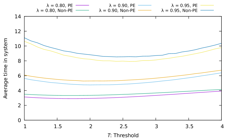
Figure 1: Performance under threshold schemes with exact information, exponentially distributed service times.

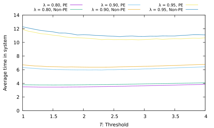
Figure 2: Performance under threshold schemes with predicted information, exponentially distributed service times, exponential predictions.

We also do experiments for the Weibull distribution with cumulative distribution $1-e^{-\sqrt{2x}}$. As a baseline, when the arrival rate is $\lambda$, the expected time a job spends in such a system in equilibrium with a FIFO queue under this Weibull distribution is $(1+\lambda)/(1-\lambda)$.

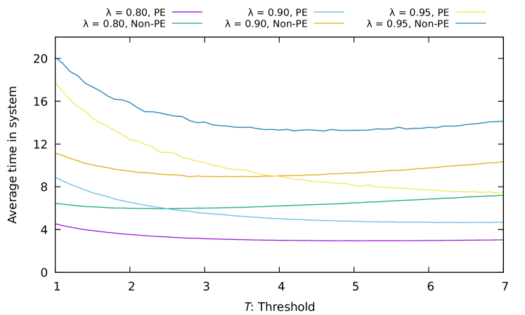
Figure 3: Performance under threshold schemes with exact information, Weibull distributed service times.

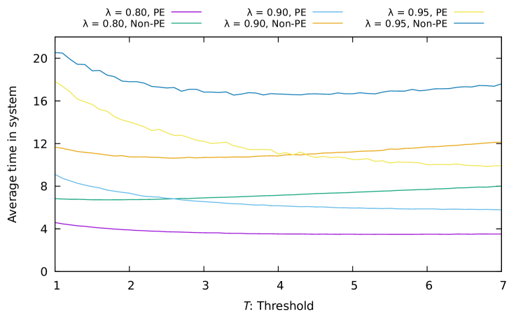
Figure 4: Performance under threshold schemes with predicted information, Weibull distributed service times, exponential predictions.

Similar to before, Figure 4 shows the results as the threshold varies given correct one-bit advice, and Figure 4 shows the results under the exponential prediction model. Note that the range of thresholds is much larger. One would expect larger thresholds would be optimal for a heavy-tailed distribution, as the downside of having a very large job at the front of the queue is more substantial. Further, in this setting, preemption offers more substantial gains, and clearly pushes the optimal threshold to larger values, as preemption significantly reduces the impact of a long job holding the queue. While the cost of using predicted advice over optimal advice is larger, the potential (and actual) gains from using predicted advice are even more substantial.

To shed additional light, we compare one-bit advice to no advice, in which case the queue uses FIFO, and full knowledge of the processing times, in which case the queue uses Shortest Remaining Processing Time (SRPT). In the case of predictions, we consider the exponential prediction model, comparing our schemes against FIFO and Shortest Predicted Remaining Processing Time [13], which uses SRPT scheduling on the predicted times. For FIFO results we simply use the standard formula for expected time in the system; we could similarly use formulae for the other results, but present results from simulations. In particular, for our one-bit schemes, we choose the best threshold from simulation result, and allow preemptions. As we can see in Tables 1 and 2, one-bit schemes greatly improve on FIFO across the board, with a greater improvement for Weibull distributions, as one would expect. Indeed, one-bit threshold schemes achieve a large fraction of the benefit that would arise from full knowledge of processing times, and one-bit predictions achieve a large fraction of the benefit that would arise from more detailed predictions. We also find that preemption is helpful, and moreso for the heavier tailed distributions, as one would expect. Perhaps most important, using predictions provides large gains, nearly as good as with exact information, showing the large potential for even simple predictions to provide large value in scheduling.

	FIFO	THRESHOLD	THRESHOLD	SRPT	PREDICTION	PREDICTION	SPRPT
$\lambda$		NO PREEMPT	PREEMPT		NO PREEMPT	PREEMPT
0.50	2.000	1.783	1.564	1.425	1.850	1.698	1.659
0.60	2.500	2.089	1.814	1.604	2.209	2.013	1.940
0.70	3.333	2.542	2.203	1.875	2.761	2.517	2.369
0.80	5.000	3.329	2.910	2.355	3.757	3.451	3.143
0.90	10.00	5.278	4.755	3.552	6.366	5.960	5.097
0.95	20.00	8.535	7.914	5.532	10.848	10.372	8.424
0.98	50.00	16.495	15.735	10.436	22.418	21.909	16.696

Table 1: Results for exponentially distributed service times. Prediction results are using exponential predictions.

	FIFO	THRESHOLD	THRESHOLD	SRPT	PREDICTION	PREDICTION	SPRPT
		NO PREEMPT	PREEMPT		NO PREEMPT	PREEMPT
0.50	4.000	3.012	1.608	1.411	3.155	1.736	1.940
0.60	5.500	3.676	1.867	1.574	3.918	2.062	2.280
0.70	8.000	4.565	2.258	1.813	4.983	2.568	2.750
0.80	13.00	5.955	2.951	2.217	6.721	3.481	3.519
0.90	29.00	8.940	4.649	3.154	10.630	5.790	5.224
0.95	58.00	13.223	7.448	4.517	16.546	9.846	7.788
0.98	148.0	22.451	15.194	7.666	29.346	20.918	13.404

Table 2: Results for Weibull distributed service times. Prediction results are using exponential predictions.

5.2 Multiple Queues

We present results here for an example using the power of two choices, to demonstrate the results from differential equations match simulations, and to show the effectiveness of working with predictions. In our example we follow the 80-20 rule; we choose parameters $\lambda_{1}=0.225$, $\mu_{1}=3.2$, $\lambda_{2}=0.90$, and $\mu_{2}=0.20$. The overall load on the system is therefore $0.9$. For simulations, each data point is obtained by simulating systems of 1000 (initially empty) queues over 100000 units of time, and taking the average response time for all jobs that terminate after time 10000. We then take the average of over 100 simulations. For the differential equations, we simply used Euler’s method over times steps of $10^{-5}$ over time $10^{4}$. (This provides an accurate calculation for the “fixed point”, or stationary distribution corresponding to the solution of these equations.) All experiments use two choices. We provide simulation results for randomly choosing a single queue and using FIFO, choosing a queue based on the least loaded and using SRPT within the queue, and choosing the shorter of two queues and FIFO processing for comparison. We provide simulation results for various predictions, where the two values after “Pred” in the table are $q_{1}$ (misprediction for long jobs) and $q_{2}$ (short jobs), respectively.

	Simulations	Diff. Eqns.
1 Choice	24.208	$---$
SRPT	2.366	$---$
Shorter Queue, FIFO	4.967	$---$
Pred 0.0, 0.0	3.394	3.392
Pred 0.1, 0.1	3.690	3.688
Pred 0.2, 0.2	4.010	4.007
Pred 0.3, 0.3	4.353	4.347
Pred 0.4, 0.4	4.717	4.711
Pred 0.5, 0.5	5.105	5.098
Pred 0.2, 0.4	4.280	4.276
Pred 0.4, 0.2	4.402	4.395
Pred 0.11, 0.61	4.617	4.611

Table 3: Results for queueing systems with 1000 queues, 2 choices and baseline comparisons.

The main takeaways from Table 3, beyond the fact that the differential equations are quite accurate (less than 0.2% difference in these examples), are that one-bit predictions can provide benefits over the already excellent performance of choosing the shorter queue; even when all predictions are only 60% accurate, we seem some gain in performance. Considering $q_{1}=0.2$ and $q_{2}=0.4$ along with $q_{1}=0.4$ and $q_{2}=0.2$ shows that predictions for long jobs are more important, even though there are much fewer long jobs. The effect of giving a long job higher priority, where it can block short jobs, has a more prominent effect than misclassifying a short job. This demonstrates that the goal of a machine learning algorithm in this setting should not be simply to maximize the number of correct predictions; a machine learning algorithm can do better by predicting the long jobs well. (See [14] for a similar discussion.)

As an extreme example of this, choosing $q_{1}=0.11$ and $q_{2}=0.61$ leads to a total error rate of 51% over all jobs, as short jobs have a much higher arrival rate than long jobs. But even though more than half the jobs types are predicted incorrectly, because long jobs are predicted correctly most of the time, such predictions still perform notably better than not using predictions and just choosing the shorter queue.

6 Conclusions

We have looked at the setting of queueing systems with one bit of advice, where a primary motivation is the potential for machine learning algorithms to provide simple but useful predictions to improve scheduling. In the case of single queues, we see that a natural probabilistic model for predictions leads to relatively straightforward equations that can be used to determine where one would ideally choose a threshold to separate long and short jobs. For large-scale queueing systems, where the power of two choices can be used, we have shown that one-bit prediction can allow for fluid limit analysis. We view this as a potential step forward for the interesting open problem of determining the behavior of systems using the power of two choices with scheduling via shortest remaining processing time or other scheduling schemes based on the service time.

We believe there remain several interesting directions to explore in this space. The use of predictions in more complex settings, such as call centers, may provide significant value. A challenging underlying questions, when “jobs” may correspond to people, is how to define appropriate notions of fairness, so tht jobs that are mispredicted by a machine learning algorithm do not suffer overly from the algorithm’s behavior.

References

- [1] Reza Aghajani, Xingjie Li, and Kavita Ramanan. Mean-field dynamics of load-balancing networks with general service distributions. arXiv preprint arXiv:1512.05056, 2015.
- [2] Yossi Azar, Andrei Z. Broder, Anna R. Karlin, and Eli Upfal. Balanced allocations. SIAM J. Comput., 29(1):180–200, 1999.
- [3] Joan Boyar, Lene M Favrholdt, Christian Kudahl, Kim S Larsen, and Jesper W Mikkelsen. Online algorithms with advice: a survey. ACM SIGACT News, 47(3):93–129, 2016.
- [4] Matteo Dell’Amico, Damiano Carra, and Pietro Michiardi. PSBS: Practical size-based scheduling. IEEE Transactions on Computers, 65(7):2199-2212, 2015.
- [5] S. N. Ethier and T. G. Kurtz. Markov Processes: Characterization and Convergence. John Wiley and Sons, 1986.
- [6] Mor Harchol-Balter. Performance modeling and design of computer systems: queueing theory in action. Cambridge University Press, 2013.
- [7] Tim Hellemans and Benny Van Houdt. On the power-of--choices with least loaded server selection. POMACS, 2(2):27:1–27:22, 2018.
- [8] Chen-Yu Hsu, Piotr Indyk, Dina Katabi, and Ali Vakilian. Learning-Based Frequency Estimation Algorithms. In 7th International Conference on Learning Representations, 2019.
- [9] Tim Kraska, Alex Beutel, Ed H Chi, Jeffrey Dean, and Neoklis Polyzotis. The case for learned index structures. In Proceedings of the 2018 International Conference on Management of Data, pages 489–504, 2018.
- [10] T. G. Kurtz. Solutions of Ordinary Differential Equations as Limits of Pure Jump Markov Processes. Journal of Applied Probability, Vol. 7, 1970, pp. 49-58.
- [11] Thodoris Lykouris and Sergei Vassilvitskii. Competitive caching with machine learned advice. In Proceedings of the 35th International Conference on Machine Learning, pp. 3302–3311, 2018.
- [12] Michael Mitzenmacher. The power of two choices in randomized load balancing. IEEE Trans. Parallel Distrib. Syst., 12(10):1094–1104, 2001.
- [13] Michael Mitzenmacher. Scheduling with predictions and the price of misprediction. 11th Innovations in Theoretical Computer Science Conference, ITCS 2020, 14:1-14:18, 2020.
- [14] Michael Mitzenmacher. The Supermarket Model with Known and Predicted Service Times. arXiv preprint arXiv:1905.12155, 2019.
- [15] Michael Mitzenmacher and Sergei Vassilvitskii. Algorithms with Predictions. In Beyond the Worst-Case Analysis of Algorithms, edited by Tim Roughgarden, Cambridge University Press, 2020.
- [16] T.M. O’Donovan. Direct solutions of M/G/1 priority queueing models. Revue française d’automatique, informatique, recherche opérationnelle, 10.V1, 107-111, 1976.
- [17] Manish Purohit, Zoya Svitkina, and Ravi Kumar. Improving online algorithms via ML predictions. In Advances in Neural Information Processing Systems, pages 9684–9693, 2018.
- [18] Nikita Dmitrievna Vvedenskaya, Roland L’vovich Dobrushin, and Fridrikh Izrailevich Karpelevich. Queueing system with selection of the shortest of two queues: An asymptotic approach. Problemy Peredachi Informatsii, 32(1):20–34, 1996.
- [19] Adam Wierman and Misja Nuyens. Scheduling despite inexact job-size information. Performance Evaluation Review, 36(1):25-36, 2008.
- [20] N.C. Wormald. Differential equations for random processes and random graphs. The Annals of Applied Probability, 5(1995), pp. 1217–1235.