Partial Factorizations of Products of Binomial Coefficients

Abstract.

Let ${\overline{G}}_{n}=\prod_{k=0}^{n}\binom{n}{k},$ the product of the elements of the $n$-th row of Pascal’s triangle. This paper studies the partial factorizations of ${\overline{G}}_{n}$ given by the product $G(n,x)$ of all prime factors $p$ of ${\overline{G}}_{n}$ having $p\leq x$, counted with multiplicity. It shows $\log G(n,\alpha n)\sim f_{G}(\alpha)n^{2}$ as $n\to\infty$ for a limit function $f_{G}(\alpha)$ defined for $0\leq\alpha\leq 1$. The main results are deduced from study of functions $A(n,x),B(n,x),$ that encode statistics of the base $p$ radix expansions of the integer $n$ (and smaller integers), where the base $p$ ranges over primes $p\leq x$. Asymptotics of $A(n,x)$ and $B(n,x)$ are derived using the prime number theorem with remainder term or conditionally on the Riemann hypothesis.

1. Introduction

Let $\overline{G}_{n}$ denote the product of the binomial coefficients in the $n$th row of Pascal’s triangle

$$\overline{G}_{n}:=\prod_{k=0}^{n}\binom{n}{k}=\frac{(n!)^{n+1}}{\prod_{k=0}^{n}(k!)^{2}}.$$ (1.1)

These products were studied in [24], where it was observed that the integer sequence ${\overline{G}}_{n}$ arises as the inverse of the product of all the non-zero unreduced Farey fractions, i.e. the set of all rational fractions in the unit interval $(0,1]$ having denominator at most $n$, not necessarily in lowest terms. We write the prime factorization of ${\overline{G}}_{n}$ as

$${\overline{G}}_{n}=\prod_{p}p^{\nu_{p}({\overline{G}}_{n})}$$ (1.2)

where $\nu_{p}({\overline{G}}_{n})={\rm ord}_{p}({\overline{G}}_{n})$. Since ${\overline{G}}_{n}$ is an integer, $\nu_{p}({\overline{G}}_{n})\geq 0$ for all $n\geq 1$. The asymptotic growth rate of ${\overline{G}}_{n}$ is easily determined, using Stirling’s formula, to be

$$\log\overline{G}_{n}=\frac{1}{2}n^{2}-\frac{1}{2}n\log n+O(n),$$ (1.3)

an estimate which is valid more generally for the step function $\overline{G}_{x}:=\overline{G}_{\lfloor x\rfloor}$ for all real $x\geq 1$. The sequence ${\overline{G}}_{n}$ considered only at integer points $n$ has a complete asymptotic expansion for $\log\overline{G}_{n}$ to all orders in $(\frac{1}{n})^{k}$ $(k\geq 0)$, see [24, Theorem A.2].)

The purpose of this paper is to study the internal structure of the prime factorization of ${\overline{G}}_{n}$ as $n$ varies, as measured by the partial factorization

$$G(n,x)=\prod_{p\leq x}p^{\nu_{p}({\overline{G}}_{n})}.$$ (1.4)

Here $G(n,x)$ is a divisor of ${\overline{G}}_{n}$ that includes the total contribution of all primes up to $x$ in the product ${\overline{G}}_{n}$. The function $G(n,x)$ for fixed $n$ is an integer-valued step function of the variable $x$. This function of $x$ stabilizes for $x\geq n$, with

$$G(n,x)=G(n,n)={\overline{G}}_{n}\quad\mbox{for}\quad x\geq n.$$

This paper determines the asymptotic behavior of $\log G(n,x)$ and related arithmetic statistics as $n\to\infty$ for a wide range of $x$, with emphasis on the range when $x\sim\alpha n$, for fixed $0<\alpha\leq 1$. To do so it determines the asymptotic behavior of auxiliary statistics $A(n,x)$ and $B(n,x)$, defined below, which encode information on radix expansions of integers up to $n$ to prime bases $p\leq n$.

1.1. Result: Asymptotics of $G(n,x)$

We determine the size of the partial factorization function $G(n,x)$ in the range $1\leq x\leq n$. We establish limiting behavior as $n\to\infty$ taking $x=x(n):=\alpha n$.

Theorem 1.1.

Let $G(n,x)=\prod_{p\leq x}p^{\nu_{p}({\overline{G}}_{n})}$. Then for all $0<\alpha\leq 1$,

$$\log G(n,\alpha n)=f_{G}(\alpha)n^{2}+R_{G}(n,\alpha n),$$ (1.5)

where $f_{G}(\alpha)$ is a function given for $\alpha>0$ by

$$f_{G}(\alpha)=\frac{1}{2}+\frac{1}{2}\alpha^{2}\left\lfloor\frac{1}{\alpha}\right\rfloor^{2}+\frac{1}{2}\alpha^{2}\left\lfloor\frac{1}{\alpha}\right\rfloor-\alpha\left\lfloor\frac{1}{\alpha}\right\rfloor,$$ (1.6)

with $f_{G}(0)=0$ and $R(n,\alpha n)$ is a remainder term.

(1) Unconditionally there is a positive constant $c$ such that for all $n\geq 4$, and all $0<\alpha\leq 1$ the remainder term satisfies

$$R_{G}(n,\alpha n)=O\left(\frac{1}{\alpha}n^{2}\exp(-c\sqrt{\log n})\right).$$ (1.7)

The implied constant in the $O$-notation does not depend on $\alpha$.

(2) Conditionally on the Riemann hypothesis, for all $n\geq 4$ and all $0<\alpha\leq 1$, the remainder term satisfies

$$R_{G}(n,\alpha n)=O\left(\frac{1}{\alpha}n^{7/4}(\log n)^{2}\right),$$ (1.8)

The implied constant in the $O$-notation does not depend on $\alpha$.

The limit function $f_{G}(\alpha)=\lim_{n\to\infty}\frac{1}{n^{2}}\log G(n,\alpha n)$ is pictured in Figure 1.

Figure 1. Graph of limit function $f_{G}(\alpha)$ in $(\alpha,\beta)$-plane for $0\leq\alpha\leq 1.$ The dotted line is $\beta=\frac{1}{2}\alpha$.

The limit function $f_{G}(\alpha)$ has the following properties (cf. Lemma 4.2).

1. The function $f_{G}$ is continuous on $[0,1]$. It has $\lim_{\alpha\to 0^{+}}f_{G}(\alpha)=0$ and the formula (1.6) gives the value $f_{G}(0)=0$, making the convention that $\alpha\lfloor\frac{1}{\alpha}\rfloor=1$ at $\alpha=0$. It is not differentiable at each point $\alpha=\frac{1}{j}$ for integer $j\geq 2$, and not differentiable from above at $\alpha=0$.

2. The function $f_{G}$ satisfies

   $$f_{G}(\alpha)\leq\frac{1}{2}\alpha\quad\mbox{for}\quad 0\leq\alpha\leq 1.$$ (1.9)

   Equality holds at $\alpha=\frac{1}{j}$ for all integer $j\geq 1$, with $f_{G}\left(\frac{1}{j}\right)=\frac{1}{2j}$, and at $\alpha=0$ (by convention) and at no other values.

Specifically $f_{G}(\alpha)$ is piecewise quadratic, i.e. for $j\geq 1$, on each closed interval $\left[\frac{1}{j+1},\frac{1}{j}\right]$ it is given by

$$f_{G}(\alpha)=\frac{1}{2}-j\alpha+\frac{j(j+1)}{2}\alpha^{2}\quad\mbox{for}\quad\frac{1}{j+1}\leq x\leq\frac{1}{j}.$$ (1.10)

Theorem 1.1 is a restated form of Theorem 4.1, which applies uniformly to the full range $1\leq x\leq n$. The new content of Theorem 1.1 concerns the range $0<\alpha<1$ and determination of the function $f_{G}(\alpha)$. At the endpoint $\alpha=1$ the binomial product estimate (1.3) gives an unconditional asymptotic formula for $\log G(n,n)$ with power-savings remainder term better than (1.8). This value $G(n,n)$ is given explicitly by a product of ratios of factorials, permitting the estimate. Improved estimates are possible in some parts of the range $x=o(n)$, corresponding to $\alpha=0$, using exponential sum methods, as discussed at the end of Section 1.2.

We now consider the methods used to prove Theorem 1.1. It is proved starting from an expression for $\log G(n,x)$ obtained taking the logarithm of the factorization (1.4):

$$\log G(n,x)=\sum_{p\leq x}\nu_{p}({\overline{G}}_{n})\log p.$$ (1.11)

The proof uses formulas for the individual exponents $\nu_{p}({\overline{G}}_{n})$ given in terms of base $p$ radix expansion data of the integers up to $n$, proved in [24] and stated in Section 1.2 below. The functions $\nu_{p}({\overline{G}}_{n})$ exhibit a kind of self-similar behavior, different for each $p$, having large fluctuations. One can write the individual exponents $\nu_{p}({\overline{G}}_{n})$ as a difference of quantities given by statistics of the base $p$ radix expansion of integers up to $n$ (see Theorem 1.3 ). Summing over $p\leq x$ yields a formula

$$\log G(n,x)=A(n,x)-B(n,x),$$

involving nonnegative arithmetic functions $A(n,x)$ and $B(n,x)$ defined in (1.17) and (1.18) below. The functions $A(n,x)$ and $B(n,x)$ encode information on prime number counts, as detailed in Section 1.5 below.

The main technical results of this paper are estimates of the the size of $A(n,x)$ and $B(n,x)$. These functions are weighted averages of statistics of the radix expansions of $n$ for varying prime bases $p\leq x$. Individual radix statistics have been extensively studied in the literature, holding the radix base $p$ fixed and varying $n$. The case of fixed $n$ and variable $p$ considered here seems not well studied.

1.2. Products of binomial coefficients and digit sum statistics

It is well known that the divisibility of binomial coefficients ${{n}\choose{k}}$ by prime powers is described by base $p$ radix expansion conditions, starting from work of Kummer, see the survey of Granville [18]. Given a base $b\geq 2$, write the base $b$ radix expansion of an integer $n\geq 0$ as

$$n=\sum_{i=0}^{k}a_{i}b^{i}\quad\mbox{with}\quad 0\leq a_{i}=a_{i}(b,n)\leq b-1,$$

in which $b^{k}\leq n<b^{k+1}$ and the top digit $a_{k}(b,n)\geq 1$. One has

$$a_{i}(b,n)=\left\lfloor\frac{n}{b^{i}}\right\rfloor-b\left\lfloor\frac{n}{b^{i+1}}\right\rfloor.$$ (1.12)

The radix conditions involve the following two statistics of the base $b$ digits of $n$.

Definition 1.2.

(1) The sum of digits function $d_{b}(n)$ (to base $b$) is

$$d_{b}(n):=\sum_{i\geq 0}a_{i}(b,n).$$ (1.13)

(2) The running digit sum function $S_{b}(n)$ (to base $b$) is

$$S_{b}(n):=\sum_{j=0}^{n-1}d_{b}(j).$$ (1.14)

The paper [24] derived a closed formula for ${\rm ord}_{p}({\overline{G}}_{n})$ which involves such radix expansions of the integers $1\leq j\leq n$.

Theorem 1.3.

([24, Theorem 5.1]) For each prime $p$ one has for each $n\geq 1$,

$$\nu_{p}({\overline{G}}_{n})=\frac{2}{p-1}S_{p}(n)-\frac{n-1}{p-1}d_{p}(n).$$ (1.15)

The formula (1.15) encodes large cancellations of powers of $p$ between the numerator and denominator of the factorial form for ${\overline{G}}_{n}$ on the right side of (1.1). The individual terms on the right side of (1.15) need not be integers: As an example, $n=35$ has base $p=7$ expansion $(50)_{7}$, whence $d_{7}(35)=5$ and $\frac{n-1}{p-1}d_{p}(n)=\frac{85}{3}$, while $\frac{2}{p-1}S_{p}(n)=\frac{175}{3}$ and $\nu_{7}({\overline{G}}_{35})=30$.

Taking logarithms of both sides of the product formula (1.4) for $G(n,x)$ and substituting the formula (1.15) for each $\nu_{p}({\overline{G}}_{n})$ yields the following identity. There holds

$$\log G(n,x)=A(n,x)-B(n,x),$$ (1.16)

where

$$A(n,x)=\sum_{p\leq x}\frac{2}{p-1}S_{p}(n)\log p$$ (1.17)

and

$$B(n,x)=\sum_{p\leq x}\frac{n-1}{p-1}d_{p}(n)\log p.$$ (1.18)

The functions $A(n,x)$ and $B(n,x)$ are arithmetical sums that combine behavior of the base $p$ digits of the integer $n$, viewing $n$ as fixed, and varying the radix base $p$. The interesting range of $x$ is $1\leq x\leq n$ because these functions “freeze” at $x=n$: $A(n,x)=A(n,n)$ for $x\geq n$ and $B(n,x)=B(n,n)$ for $x\geq n$.

We single out the special case $x=n$, setting

$$A(n):=A(n,n)=\sum_{p\leq n}\frac{2}{p-1}S_{p}(n)\log p$$ (1.19)

and

$$B(n):=B(n,n)=\sum_{p\leq n}\frac{n-1}{p-1}d_{p}(n)\log p.$$ (1.20)

The sums $A(n)$ and $B(n)$ hold $n$ fixed and vary the base $p$.

The main results of the paper estimate the functions $A(n,x),B(n,x)$ and $\log G(n,x)$ for $1\leq x\leq n$ with main terms having the general form $f(\alpha)n^{2}$ where $\alpha=\frac{x}{n}$ and with such $f(\alpha)$ for $0\leq\alpha\leq 1$ is a continuous function having $f(0)=0$. The proofs first estimate $A(n,n)$ and $B(n,n)$, and then use these estimates as input to recursively estimate $A(n,x)$ and $B(n,x)$ for general $x$.

Olivier Bordellès informed us that exponential sum methods yield alternative unconditional estimates for $A(n,x)$, $B(n,x)$ and $\log G(n,x)$, which are nontrivial when $x=o(n)$, and apply for $x>\sqrt{n}$. These estimates improve on the estimates of our main theorems for certain ranges of $x$. We present such estimates in Appendix A. The main terms in the exponential sum estimates have a different form than the main terms in the estimates for $A(n,x)$, $B(n,x)$ and $\log G(n,x)$. Theorem 3.7 obtains for $x=o(n)$ a simplified form of our main terms which facilitates a comparison of the estimates.

1.3. Results: Asymptotics of $A(n)$ and $B(n)$

We determine asymptotics of the two functions $A(n)$ and $B(n)$ as $n\to\infty$, giving a main term and a bound on the remainder term. The analysis proceeds by estimating the fluctuating term $B(n)$ depending on $d_{p}(n)$.

Theorem 1.4.

Let $A(n)=\sum_{p\leq n}\frac{2}{p-1}S_{p}(n)\log p$ and $B(n)=\sum_{p\leq n}\frac{n-1}{p-1}d_{p}(n)\log p.$

(1) There is a constant $c>0$, such that for $n\geq 4$,

$$A(n)=\left(\frac{3}{2}-\gamma\right)n^{2}+O\left(n^{2}\exp(-c\sqrt{\log n})\right),$$ (1.21)

where $\gamma$ denotes Euler’s constant. Similarly

$$B(n)=(1-\gamma)n^{2}+O\left(n^{2}\exp(-c\sqrt{\log n})\right).$$ (1.22)

(2) Assuming the Riemann hypothesis, for all $n\geq 4$,

$$A(n)=\left(\frac{3}{2}-\gamma\right)n^{2}+O\left(n^{7/4}(\log n)^{2}\right).$$ (1.23)

and

$$B(n)=(1-\gamma)n^{2}+O\left(n^{7/4}(\log n)^{2}\right),$$ (1.24)

Theorem 1.4 answers a question raised in [24, Section 8] of whether the asymptotic growth of $A(n)$ is the same as that of the sum $A^{\ast}(n)$ obtained by replacing each $S_{p}(n)$ with the leading term of its asymptotic growth estimate as $n\to\infty$. They are not the same: see Section 1.5.

To establish Theorem 1.4 it suffices to prove it for $B(n)$; the estimate for $A(n)$ then follows from the linear relation $A(n)=\log{\overline{G}}_{n}+B(n)$ (from (1.16)) combined with the asymptotic estimate for $G(n)$ in (1.3). The main contribution in the sum $B(n)$ comes from those primes $p$ having $p>\sqrt{n}$, whose key property is that : their base $p$ radix expansions have exactly two digits. The size of the remainder term then involves prime counting functions, which relate to the zeros of the Riemann zeta function. We obtain an unconditional result from the standard zero-free region for $\zeta(s)$. The Riemann hypothesis, or more generally a zero-free region for the zeta function of the form $Re(s)>1-c_{0}$ for some $c_{0}>0$ yields an asymptotic formula of shape $B(n)=(1-\gamma)n^{2}+O\left(n^{2-\delta}\right)$ with a power-saving remainder term $\delta=\delta(c_{0})$ depending on the width of the zero-free region.

The constants appearing in the main terms of the asymptotics of $A(n)$ and $B(n)$ in Theorem 1.4 give quantitative information on cross-correlations between the statistics $d_{p}(n)$ and $S_{p}(n)$ of the base $p$ digits of $n$ (and smaller integers) as the base $p$ varies while $n$ is held fixed. As suggested in the survey [23], the occurrence of Euler’s constant in the main term of these asymptotic estimates encodes subtle arithmetic behavior in these sums.

1.4. Results: Asymptotics of $A(n,x)$ and $B(n,x)$

We first determine asymptotics for $B(n,\alpha n)$ for $0\leq\alpha\leq 1$, starting from $B(n)=B(n,n)$ and obtaining $B(n,x)$ by decreasing $x$ from $x=n$. In what follows $H_{m}=\sum_{j=1}^{m}\frac{1}{j}$ denotes the $m$-th harmonic number and $\gamma$ denotes Euler’s constant.

Theorem 1.5.

Let $B(n,\alpha n)=\sum_{p\leq\alpha n}\frac{n-1}{p-1}d_{p}(n)\log p.$ Then for all $0<\alpha\leq 1$,

$$B(n,\alpha n)=f_{B}(\alpha)n^{2}+R_{B}(n,\alpha n),$$ (1.25)

where $f_{B}(\alpha)$ is a function given for $\alpha>0$ by

$$f_{B}(\alpha)=1-\gamma+\left(H_{\lfloor\frac{1}{\alpha}\rfloor}-\log\frac{1}{\alpha}\right)-\alpha\left\lfloor\frac{1}{\alpha}\right\rfloor,$$ (1.26)

with $f_{B}(0)=0$, and $R_{B}(n,\alpha n)$ is a remainder term.

(1) Unconditionally there is a positive constant $c$ such that for all $n\geq 4$, and $0<\alpha\leq 1$, the remainder term satisfies

$$R_{B}(n,\alpha n)=O\left(\frac{1}{\alpha}n^{2}\exp(-c\sqrt{\log n})\right).$$ (1.27)

The implied constant in the $O$-notation does not depend on $\alpha$.

(2) Conditionally on the Riemann hypothesis, for all $n\geq 4$ and $0<\alpha\leq 1$, the remainder term satisfies

$$R_{B}(n,\alpha n)=O\left(\frac{1}{\alpha}n^{7/4}(\log n)^{2}\right),$$ (1.28)

The implied constant in the $O$-notation does not depend on $\alpha$.

The limit function $f_{B}(\alpha)$ is pictured in Figure 2. The function lies strictly above the diagonal line $\beta=(1-\gamma)\alpha$; note that in (1.16) in its relation to $\log G(n,x)$ it appears with a negative sign, consistent with $f_{G}(\alpha)\leq\frac{1}{2}\alpha$.

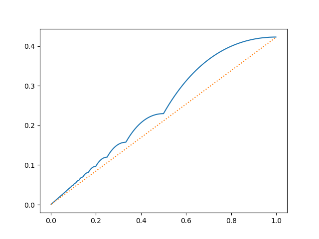
Figure 2. Graph of limit function $f_{B}(\alpha)$ in $(\alpha,\beta)$-plane, $0\leq\alpha\leq 1.$ The dotted line is $\beta=(1-\gamma)\alpha$, where $\gamma$ is Euler’s constant.

We then obtain asymptotics for $A(n,x)$ using a recursion starting from $A(x,x)$ (given by (3.14)) relating $A(n,x)$ to various $B(y,x)$ with $x\leq y\leq n$.

Theorem 1.6.

Let $A(n,\alpha n)=\sum_{p\leq\alpha n}\frac{2}{p-1}S_{p}(n)\log p.$ Then for all $0<\alpha\leq 1$,

$$A(n,\alpha n)=f_{A}(\alpha)n^{2}+R_{A}(n,\alpha n),$$ (1.29)

where $f_{A}(\alpha)$ is a function given for $\alpha>0$ by

$$f_{A}(\alpha)=\frac{3}{2}-\gamma+\left(H_{\left\lfloor\frac{1}{\alpha}\right\rfloor}-\log\frac{1}{\alpha}\right)+\frac{1}{2}\alpha^{2}\left\lfloor\frac{1}{\alpha}\right\rfloor^{2}+\frac{1}{2}\alpha^{2}\left\lfloor\frac{1}{\alpha}\right\rfloor-2\alpha\,\left\lfloor\frac{1}{\alpha}\right\rfloor,$$ (1.30)

with $f_{A}(0)=0$, and $R_{A}(n,\alpha n)$ is a remainder term.

(1) Unconditionally there is a positive constant $c$ such that for all $n\geq 4$, and $0<\alpha\leq 1$. the remainder term satisfies

$$R_{A}(n,\alpha n)=O\left(\frac{1}{\alpha}n^{2}\exp(-c\sqrt{\log n})\right).$$ (1.31)

The implied constant in the $O$-notation does not depend on $\alpha$.

(2) Conditionally on the Riemann hypothesis, for all $n\geq 4$ and $0<\alpha\leq 1$, the remainder term satisfies

$$R_{A}(n,\alpha n)=O\left(\frac{1}{\alpha}n^{7/4}(\log n)^{2}\right),$$ (1.32)

The implied constant in the $O$-notation does not depend on $\alpha$.

The limit function $f_{A}(\alpha)$ is pictured in Figure 3. It lies very close to the line $\beta=(3/2-\gamma)\alpha$. The graph of $f_{A}(\alpha)$ falls below the line $\beta=(3/2-\gamma)\alpha$ for $\alpha>\alpha_{0}$ and falls above it for $\alpha<\alpha_{0}$, with $\alpha_{0}\approx 0.82$. The figure also depicts a plot of its derivative $f_{A}^{{}^{\prime}}(\alpha)$, with horizontal dotted line indicating derivative $\frac{3}{2}-\gamma$.

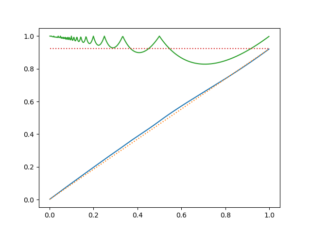
Figure 3. Graph of limit function $f_{A}(\alpha)$ in $(\alpha,\beta)$-plane, $0\leq\alpha\leq 1.$ The dotted line is $\beta=(3/2-\gamma)\alpha$, where $\gamma$ is Euler’s constant. Superimposed on the graph is a plot of the derivative $f_{A}^{{}^{\prime}}(\alpha)$ drawn to the same scale.

We note that the functions $f_{A}(\alpha)$ and $f_{B}(\alpha)$ are continuous functions of $\alpha$, although the given floor function formulas for $f_{A}(\alpha)$ and $f_{B}(\alpha)$ are a sum of functions that are discontinuous at the points $\alpha=\frac{1}{k}$.

Theorem 1.5 and Theorem 1.6 are restated versions of Theorems 3.1 and Theorem 3.4 given in terms of the $x$-variable. Theorem 1.1 follows as a corollary of these two theorems, substituting their estimates into the formula $\log G(n,x)=A(n,x)-B(n,x)$. In the subtraction giving the asymptotics of $\log G(n,x)$, Euler’s constant cancels out.

1.5. Motivation: Digit sum statistics and the prime number theorem

The statistics $A(n,x)$ and $B(n,x)$ can be related to the problem of estimating $\pi(x)$.

1.5.1. Running digit sum $S_{b}(n)$

The radix statistic $S_{b}(n)$ a fixed integer base $b\geq 2$ has been extensively studied. It was treated in 1940 by Bush [2], followed by Bellman and Shapiro [1], and Mirsky [29], who in 1949 showed that for all $b\geq 2$,

$$S_{b}(n)=n\log_{b}(n)+O_{b}(n),$$ (1.33)

where the implied constant in the $O$-notation depends on the base $b$. In 1952 Drazin and Griffith [9] deduced an inequality implying that for all bases $b\geq 2$,

$$S_{b}(n)\leq\frac{b-1}{2}n\log_{b}n\quad\mbox{ for all}\quad n\geq 1,$$ (1.34)

with equality holding for $n=b^{k}$ for $k\geq 1$, cf. [24, Theorem 5.8]. The upper bound (1.34) suggests consideration of the statistic

$$A^{\ast}(n,x):=\sum_{p\leq x}\frac{2}{p-1}\left(\frac{p-1}{2}n\log_{p}n\right)\log p=\pi(x)\,n\log n.$$ (1.35)

Applying inequality (1.34) for $S_{p}(n)$ term-by-term to the definition of $A(n,x)$ yields

$$A(n,x)\leq A^{\ast}(n,x)=\pi(x)n\log n.$$ (1.36)

Furthermore from the estimate (1.33) applied term-by-term to the definition of $A(n,x)$, we obtain, viewing $x$ as fixed and $n$ as varying.

$$A(n,x)=\pi(x)n\log n+O_{x}(n),$$ (1.37)

where the implied constant in the $O$-symbol depends on $x$. It follows that for fixed $x$ one has the the asymptotic formula

$$A(n,x)\sim A^{\ast}(n,x)=\pi(x)\,n\log n\quad\mbox{as}\quad n\to\infty,$$ (1.38)

Thus $A(n,x)$ encodes information about $\pi(x)$ for $n$ very large compared to $x$. In the case where $x=n$ (1.36) gives

$$A(n)=A(n,n)\leq A^{\ast}(n,n)=\pi(n)n\log n.$$ (1.39)

The prime number theorem estimate $\pi(n)=\frac{n}{\log n}+O\left(\frac{n}{(\log n)^{2}}\right)$ yields

$$\pi(n)n\,\log n=n^{2}+O\left(\frac{n^{2}}{\log n}\right).$$

The question of whether $A(n)\sim A^{\ast}(n,n)$ could hold as $n\to\infty$, was raised in [24, Sect. 8]. By the prime number theorem it is equivalent to the question whether $A(n)\sim n^{2}$ as $n\to\infty$. Theorem 1.4 answers this question in the negative, showing that $A(n)\sim\left(\frac{3}{2}-\gamma\right)n^{2}$, with $\frac{3}{2}-\gamma\approx 0.92288$.

1.5.2. Digit sums $d_{b}(n)$

The digit sums $d_{b}(n)$ are oscillatory quantities that have been modeled probabilistically, where one samples for a fixed $b$, the values $d_{b}(k)$ uniformly in a certain range of $k$. One has for each $n\geq 1$ the inequality

$${\mathbb{E}}[d_{b}(k):1\leq k\leq n-1]=\frac{1}{n-1}S_{b}(n),$$

and it follows that

$${\mathbb{E}}[d_{b}(k):0\leq k\leq n-1]=\frac{b-1}{2}\log_{b}n+O_{b}(1),$$ (1.40)

according to (1.33). Furthermore the bound (1.34) gives

$${\mathbb{E}}[d_{b}(k):0\leq k\leq n-1]\leq\frac{b-1}{2}\log_{b}n,$$ (1.41)

The statistic $B(n,x)$ averages over $\frac{n-1}{p-1}d_{p}(n)\log p$ holding $n$ fixed and varying $p$. Now (1.41) gives

$$\frac{n-1}{b-1}{\mathbb{E}}[d_{b}(k):0\leq k\leq n-1]\log b\leq\frac{1}{2}\log n.$$

If the averaging over $p$ in $d_{p}(n)$ in this statistic behaved similarly to averaging over $n$ for fixed $n$, then we might expect $B(n,x)$ to behave similarly to the statistic

$$B^{\ast}(n,x):=\sum_{p\leq x}\frac{n-1}{p-1}\left(\frac{p-1}{2}\log_{p}(n)\right)\log p=\frac{1}{2}\pi(x)n\log n.$$ (1.42)

The prime number theorem yields the estimate

$$B^{\ast}(n,n)=\frac{1}{2}n^{2}+O\left(\frac{n^{2}}{\log n}\right).$$

The question whether $B(n)\sim B^{\ast}(n,n)$ holds as $n\to\infty$ is equivalent to whether $B(n)\sim\frac{1}{2}n^{2}$ as $n\to\infty$ holds. Theorem 1.4 answers this question in the negative, with $B(n)=(1-\gamma)n^{2}$ as $n\to\infty$ and $1-\gamma\approx 0.42288$.

1.5.3. Asymptotics for $A(n,x)$ and $B(n,x)$ with $x=o(n)$

The estimates for $A(n,n)$ and $B(n,n)$ reveal a difficulty in deducing the prime number theorem from radix expansion statistics, purely from knowing the limiting statistics as $n\to\infty$ holding $p$ fixed. Theorem 1.4 shows that the problem is that the contributions of individual primes $p$ in these radix expansion statistics have not reached their individual limiting asymptotics as $n\to\infty$, holding $p$ fixed. In addition, when $x=\alpha n$ and $n\to\infty$, the formulas for $f_{A}(\alpha)$ and $f_{B}(\alpha)$ exhibit oscillations in the main terms of the estimates for $A(n,x)$ and $B(n,x)$.

In contrast we show that for certain ranges of relatively large $x=o(n)$ the asymptotic formula $A(n,x)\sim A^{\ast}(n,x)$ is valid.

Theorem 1.7.

Suppose that a sequence $(n_{j},x_{j})$ with $1\leq x_{j}\leq n_{j}$ having $n_{j}\to\infty$ as $j\to\infty$ satisfies the two conditions

$$\lim_{j\to\infty}\frac{x_{j}}{n_{j}}=0\quad\mbox{and}\quad\lim_{j\to\infty}\frac{\log x_{j}}{\log n_{j}}=1.$$ (1.43)

Then,

$$A(n_{j},x_{j})\sim A^{\ast}(n_{j},x_{j}):=\pi(x_{j})n_{j}\log n_{j}\quad\mbox{as}\quad j\to\infty,$$ (1.44)

and

$$\,\,\,B(n_{j},x_{j})\sim B^{\ast}(n_{j},x_{j}):=\frac{1}{2}\pi(x_{j})n_{j}\log n_{j}\quad\mbox{as}\quad j\to\infty.$$ (1.45)

In consequence

$$\log G(n_{j},x_{j})\sim\frac{1}{2}\pi(x_{j})n_{j}\log n_{j}\quad\mbox{as}\quad j\to\infty$$ (1.46)

Theorem 1.7 is proved in Section 3.3. The asymptotic formulas of Theorem 1.7 fail to hold. for values of $x$ smaller than (1.43) relative to $n$ For example, taking $x_{j}=n_{j}^{\alpha}$ for any fixed $\alpha$ with $2/3<\alpha<1$ the right side of (1.44) is $A^{\ast}(n_{j},x_{j})\sim\frac{1}{\alpha}n_{j}x_{j}$ but Theorem A.2 combined with the prime number theorem $\vartheta(x)\sim x$ shows the left side of (1.44) is $A(n_{j},x_{j})\sim n_{j}x_{j}$ in this range. Also $B^{\ast}(n_{j},x_{j})\sim\frac{1}{\alpha}n_{j}x_{j}$ while Theorem A.1 and the prime number theorem show $B(n_{j},x_{j})\sim\frac{1}{2\alpha}n_{j}x_{j}$.

1.6. Related work

Binomial coefficients and their factorizations have been studied in prime number theory and in sieve methods. In 1932 in one of his first papers Erdős [12] used the central binomial coefficients ${{2n}\choose{n}}$ to get an elegant proof of Bertand’s postulate, asserting that there exists a prime between $n$ and $2n$, as well as Chebyshev type estimates for $\pi(x)$ ([3]). Later Erdős showed with Kalmar in 1937 that such an approach could in principle yield the prime number theorem, in the sense that suitable (multiplicative) linear combinations of factorials exist to give a sharper sequence of inequalities yielding the result. However their proof of the existence of such identities assumed the prime number theorem to be true. The proof with Kalmar was lost, but in 1980 Diamond and Erdős [7] reconstructed a proof. For Erdős’s remarks on the work with Kalmar see [14, pp. 58–59] and Rusza [33, Section 1]. We mention also that the internal structure of prime factors of the middle binomial coefficient ${{2n}\choose{n}}$ has received detailed study, see Erdős et al [13] and Pomerance [31].

An earlier paper of the second author and Mehta [24] studied products of unreduced Farey fractions, and in it expressed $\log{\overline{G}}_{n}$ in terms of radix digit statistics $A(n)$ and $B(n)$. Another paper [25] studied parallel questions for products of Farey fractions, which were related to questions in prime number theory. On digit sums $S_{b}(n)$, a formula of Trollope [36] found in 1968 for base $2$ led to notable work of Delange [5], giving an exact formula for $S_{b}(n)$ for all $b\geq 1$. It asserts that, for a general base $b\geq 2$,

$$S_{b}(n)=\frac{b-1}{2}n\log_{b}(n)+f_{b}(\log_{b}n)n$$ (1.47)

where $f_{b}(x)$ is a continuous function, periodic of period $1$, which is everywhere non-differentiable. Substituting $n=1$ gives $f_{b}(0)=0$, and the inequality (1.34) implies that $f_{b}(x)\leq 0$ for all real $x$. Further work on $S_{b}(n)$ includes Flajolet et al [15] and Grabner and Hwang [16], discussed in a survey of Drmota and Grabner [10]. For work on the distribution of digit sums $d_{b}(n)$, see the survey of Chen et al [4].

Up to now direct information on sums over radix expansions like $A(n)$ or $B(n)$ has not been not been successfully used to obtain proofs of the prime number theorem. The appearance of Euler’s constant in their asymptotics connects to many problems in number theory, cf. [23]. The prime number theorem has been successfully deduced by elementary methods. In 1945 Ingham [22] deduced the prime number theorem from a Tauberian theorem starting from asymptotic estimates of

$$F(x)=\sum_{n\leq x}f\left(\frac{x}{n}\right),$$

under the Tauberian condition that $f(x)$ is positive and increasing. The prime number theorem was deduced from estimates of $\log n!$, by N. Levinson [27] in 1964 by a related method. These methods obtain a remainder term saving at most one logarithm. In 1970 Diamond and Steinig [8] obtained by elementary methods a proof of the prime number theorem with a remainder term $O\large(x\exp(-c(\log x)^{\beta})\large)$ for $\beta=\frac{1}{7}+\epsilon$. The exponent was improved to $\beta=\frac{1}{6}-\epsilon$ by Lavrik and Sobirov [26]. In 1982 Diamond [6] gave a useful survey of such approaches to the prime number theorem.

1.7. Contents of paper

Section 2 derives estimates of $A(n)$ and $B(n)$. Section 3 derives estimates of $A(n,x)$ and $B(n,x)$, and proves Theorem 1.7. In addition Theorem 3.7 in Section 3.3 gives simplified formulas for the main terms in the asymptotics of $A(n,x)$ and $B(n,x)$ which apply when $x=o(n)$. Section 4 derives estimates of $\log G(n,x)$. and proves properties of the limit functions $f_{G}(\alpha)$. Section 5 determines the limit function $f_{BC}(\alpha)$ for partial factorizations of the central binomial coefficients ${{2n}\choose{n}}$. Appendix A presents estimates for $B(n,x)$ based on exponential sums due to O. Bordellés, yielding improved estimations for $A(n,x)$, $B(n,x)$, $\log G(n,x)$ for some ranges of $x=o(n)$.

Acknowledgments

We thank Olivier Bordellès for communicating the exponential sum estimates given in Theorem A.1. of the Appendix. We are indebted to D. Harry Richman for providing plots of the limit functions, and to Wijit Yangjit for helpful comments. We thank the reviewer for references and significant simplifications of proofs. Theorem 1.4 appears in the PhD. thesis of the first author ([11]), who thanks Trevor Wooley for helpful comments. The first author was partly supported by NSF grant DMS-1701577. The second author was partly supported by NSF grants DMS-1401224 and DMS-1701576, and by a Simons Fellowship in Mathematics in 2019.

2. Asymptotics for the sums $B(n)$ and $A(n)$

In this section we first obtain asymptotics for the functions $B(n)=\sum_{p\leq n}\frac{n-1}{p-1}d_{p}(n)\log p$, given in Theorem 1.4(2). At the the end we deduce asymptotics for $A(n)=\sum_{p\leq n}\frac{2}{p-1}S_{p}(n)\log p$.

2.1. Preliminary Reduction

We study $B(n)$ and reduce the main sum to primes in the range $\sqrt{n}<p\leq n$. We write

$$B(n)=B_{1}(n)+B_{R}(n)$$ (2.1)

where

$$B_{1}(n):=\sum_{\sqrt{n}<p\leq n}\frac{n-1}{p-1}d_{p}(n)\log p$$ (2.2)

and

$$B_{R}(n):=\sum_{1<p\leq\sqrt{n}}\frac{n-1}{p-1}d_{p}(n)\log p.$$ (2.3)

is a remainder term coming from small $p$ (relative to $n$) that makes a negligible contribution to the asymptotics

Lemma 2.1.

For $n\geq 2$

$$B_{R}(n)\leq 4\,n^{3/2}.$$ (2.4)

Proof.

One has $d_{p}(n)\leq(p-1)\left(\frac{\log n}{\log p}+1\right).$ Consequently

$$B_{R}(n) \leq\sum_{p\leq\sqrt{n}}(n-1)(\log n+\log p)$$

$$\leq\sum_{p\leq\sqrt{n}}(n-1)(\log n+\log\sqrt{n})$$

$$\leq\frac{3}{2}n\pi(\sqrt{n})\log n$$

$$\leq 4\,n^{3/2},$$

The rightmost inequality used the estimate, valid for $x>1$, that

$$\pi(x)\leq 1.25506\frac{x}{\log x},$$ (2.5)

see Rosser and Schoenfeld [32, eqn. (3.6)]. ∎

2.2. Estimate for $B_{1}(n)$: radix expansion

We estimate $B_{1}(n)$ starting from the observation that for primes $\sqrt{n}<p\leq n$, the base $p$ radix expansion of $n$ for $\sqrt{n}<p\leq n$, has exactly $2$ digits.

Lemma 2.2.

For $n\geq 2$ and all primes $\sqrt{n}<p\leq n$, one has

$$d_{p}(n)=n-(p-1)\left\lfloor\frac{n}{p}\right\rfloor.$$

In consequence for all primes $\sqrt{n}<p\leq n$ lying in the interval $I_{j}=(\frac{n}{j+1},\frac{n}{j}]$, where $j=\lfloor\frac{n}{p}\rfloor$, and $1\leq j<\sqrt{n}$, one has

$$\frac{n-1}{p-1}d_{p}(n)\log p=(n-1)\left(\frac{n\log p}{p-1}-j\log p\right).$$ (2.6)

Proof.

For $\sqrt{n}<p<n$ the integer $n$ has exactly two base $p$ digits, $n=a_{1}p+a_{0}$. Here $a_{1}(n)=\lfloor\frac{n}{p}\rfloor$, corresponding to $p\in I_{j}=(\frac{n}{j+1},\frac{n}{j}]$, the trailing digit $a_{0}(n)=n-p\lfloor\frac{n}{p}\rfloor$ , whence

$$d_{p}(n)=a_{0}(n)+a_{1}(n)=(n-p\lfloor\frac{n}{p}\rfloor)+\lfloor\frac{n}{p}\rfloor=n-(p-1)\lfloor\frac{n}{p}\rfloor.$$

This formula is a special case of $d_{p}(n)=n-(p-1)\left(\sum_{k=1}^{\infty}\lfloor\frac{n}{p^{k}}\rfloor\right)$, which follows from computing $\nu_{p}(n!)$ two ways, the first being the Legendre formula $\nu_{p}(n!)=\sum_{k=1}^{\infty}\lfloor\frac{n}{p^{k}}\rfloor$ and the second being $\nu_{p}(n!)=\frac{n-d_{p}(n)}{p-1}$, see Hasse [21, Chap. 17, sect. 3].

Now the condition $j=\lfloor\frac{n}{p}\rfloor$ corresponds to $p\in I_{j}=(\frac{n}{j+1},\frac{n}{j}]$, and (2.6) follows by substitution of the value of $d_{p}(n)$ when $p>\sqrt{(}n)$. Note that the intervals $I_{j}$ for $1\leq j<\sqrt{n}$ cover the entire interval $\sqrt{n}<p\leq n$ (and may include some $p\leq\sqrt{n}$ in the last interval, where $n$ has three digits in its base $p$ radix expansion). ∎

We use the identity (2.6) to split the sum $B_{1}(n)$ into two parts:

$$B_{1}(n)=B_{11}(n)-B_{12}(n),$$ (2.7)

in which

$$B_{11}(n):=n(n-1)\sum_{\sqrt{n}<p\leq n}\frac{\log p}{p-1},$$ (2.8)

and

$$B_{12}(n):=(n-1)\sum_{j=1}^{\lfloor\sqrt{n}\,\rfloor}\,j\Bigg{[}\sideset{}{{}^{\prime}}{\sum}_{\frac{n}{j+1}<p\leq\frac{n}{j}}\log p\Bigg{]}.$$ (2.9)

where the prime in the inner sum means only $p>\sqrt{n}$ are included. (The prime only affects one term in the sum.) The sums $B_{11}(n)$ and $B_{12}(n)$ are of comparable sizes, on the order of $n^{2}$. We estimate them separately.

2.3. Estimate for $B_{11}(n)$

The first quantity $B_{11}(n)$ is a standard sum in number theory.

Theorem 2.3.

Let

$$B_{11}(n)=n(n-1)\sum_{\sqrt{n}<p\leq n}\frac{\log p}{p-1}.$$

(1) There is an absolute constant $c>0$ such that for $n\geq 4$,

$$B_{11}(n)=\frac{1}{2}n^{2}\log(n)+O(n^{2}e^{-c/2\,\sqrt{\log n}}).$$ (2.10)

(2) Assuming the Riemann hypothesis we have

$$B_{11}(n)=\frac{1}{2}n^{2}\log(n)+O\left(n^{7/4}(\log n)^{2}\right).$$ (2.11)

We prove this result after a series of preliminary lemmas. As a first reduction, we show that $\frac{\log p}{p-1}$ may be approximated by $\frac{\log p}{p}$. with a power savings error for $p>\sqrt{n}.$

Lemma 2.4.

We have, unconditionally,

$$\sum_{\sqrt{n}<p\leq n}\frac{\log p}{p-1}=\sum_{\sqrt{n}<p\leq n}\frac{\log p}{p}+O\left(\frac{1}{\sqrt{n}}\right).$$ (2.12)

Proof.

We have

$$\sum_{\sqrt{n}<p\leq n}\left(\frac{\log p}{p-1}-\frac{\log p}{p}\right) = \sum_{\sqrt{n}<p\leq n}\frac{\log p}{p(p-1)}\leq 2\sum_{\sqrt{n}<p\leq n}\frac{\log p}{p^{2}}=O\left(\frac{1}{\sqrt{n}}\right)$$

as required. ∎

To estimate the sum on the right side of (2.12), we study $h(n):=\sum_{p\leq n}\frac{\log p}{p}$. Merten’s first theorem says that the function $h(n)=\log n+O(1)$ (see [20, Theorem 425], [35, Sect. I.4]). Here we need an estimate with a better remainder term.

Lemma 2.5.

(1) There is a constant $c_{2}=\gamma-c_{1}$, where $c_{1}=\sum_{p}\sum_{k=2}^{\infty}\frac{\log p}{p^{k}}$ such that, for $x\geq 4$,

$$h(x):=\sum_{p\leq x}\frac{\log p}{p}=\log x+c_{2}+O\left(e^{-c\sqrt{\log x}}\right),$$

(2) Assuming the Riemann hypothesis, for $x\geq 4$,

$$h(x):=\sum_{p\leq x}\frac{\log p}{p}=\log x+c_{2}+O\left(x^{-1/2}(\log x)^{2}\right),$$

Proof.

(1) This result appears in Rosser and Schoenfeld [32, eqn. (2.31)].

(2) This result appears in Schoenfeld [34, eqn. (6.22)]. ∎

Definition 2.6.

(1) The first Chebyshev function $\vartheta(n)$, is defined by

$$\vartheta(n)=\sum_{p\leq n}\log p.$$

(2) The second Chebyshev function $\psi(n)$ is defined by

$$\psi(n)=\sum_{{p,\,k}\atop{p^{k}\leq n}}\log p=\sum_{m=1}^{n}\Lambda(m).$$

Here $\psi(n)=\vartheta(n)+\vartheta(n^{1/2})+\vartheta(n^{1/3})+\cdots.$ Using the Chebyshev style estimate $\vartheta(n)\leq 5n$ given in (2.5), one has

$$\vartheta(n)\leq\psi(n)\leq\vartheta(n)+5\sqrt{n}\log n.$$

We recall known bounds for $\vartheta(n)$.

Lemma 2.7.

(Chebyshev function estimates)

(1) There is a constant $c>0$ such that, for $x\geq 4$,

$$\vartheta(x)=\sum_{p\leq x}\log p=x+O\left(xe^{-c\sqrt{\log x}}\right),$$

(2) Assuming the Riemann hypothesis, for $x\geq 4$,

$$\vartheta(x)=\sum_{p\leq x}\log p=x+O\left(\sqrt{x}(\log x)^{2}\right),$$

Proof.

(1) is given in [30, Theorem 6.9].

(2) is given in [30, Theorem 13.1]. ∎

Proof of Theorem 2.3..

Recall $B_{11}(n)=n(n-1)\left(\sum_{\sqrt{n}<p\leq n}\frac{\log p}{p-1}\right)$.

(1) Applying estimate (1) of Lemma 2.5 with $x=n$ and with $x=\sqrt{n}$, subtracting the latter cancels the constant $C_{1}$ and yields

$$\sum_{\sqrt{n}<p\leq n}\frac{\log p}{p}=\log n-\frac{1}{2}\log n+O\left(e^{-c\sqrt{1/2\log n}}\right).$$

Combining this bound with Lemma 2.4 yields

$$\sum_{\sqrt{n}<p\leq n}\frac{\log p}{p-1}=\frac{1}{2}\log n+O\left(e^{-\frac{c}{2}\sqrt{\log n}}\right).$$

Multiplying by $n(n-1)$, we obtain the bound (2.10).

(2) Assuming the Riemann hypothesis, we proceed the same way as above, using the Riemann hypothesis estimate (2) of Lemma 2.5 in place of (1). ∎

2.4. Estimates for $B_{12}(n)$

We estimate $B_{12}(n)$ by rewriting it in terms of Chebyshev summatory functions, and using known estimates.

Theorem 2.8.

Let

$$B_{12}(n):=(n-1)\sum_{j=1}^{\lfloor\sqrt{n}\rfloor}j\Bigg{[}\sideset{}{{}^{\prime}}{\sum}_{\frac{n}{j+1}<p\leq\frac{n}{j}}\log p\Bigg{]}.$$

Then:

(1) There is an absolute constant $c>0$ such that for all $n\geq 4$,

$$B_{12}(n)=\frac{1}{2}n^{2}\log n+(\gamma-1)n^{2}+O\left(n^{2}\,\log n\,e^{-c/2\,\sqrt{\log n}}\right)$$ (2.13)

(2) Assuming the Riemann hypothesis we have, for all $n\geq 4$,

$$B_{12}(n)=\frac{1}{2}n^{2}\log(n)+(\gamma-1)n^{2}+O\left(n^{7/4}(\log n)^{2}\right).$$ (2.14)

Proof.

(1) We have

$$\frac{1}{n-1}B_{12}(n) =\sum_{j=1}^{\lfloor\sqrt{n}\rfloor}j\Bigg{[}\sideset{}{{}^{\prime}}{\sum}_{\frac{n}{j+1}<p\leq\frac{n}{j}}\log p\Bigg{]}$$

$$=\sum_{j=1}^{\lfloor\sqrt{n}\rfloor}j\left(\vartheta\left(\frac{n}{j}\right)-\vartheta\left(\frac{n}{j+1}\right)\right)+O\left(\sqrt{n}\log n\right)$$

$$=\left(\sum_{j=1}^{\lfloor\sqrt{n}\rfloor}\vartheta\left(\frac{n}{j}\right)\right)-(\sqrt{n}-1)\vartheta(\sqrt{n})+O\left(\sqrt{n}\log n\right)$$

where $\vartheta(m)=\sum_{p\leq m}\log p$ is the first Chebyshev summatory function, and the error estimate comes from not counting primes $p\leq\sqrt{n}$ inside the term with $j\leq\sqrt{n}<j+1$.

Using Lemma 2.7, for $j\leq\sqrt{n}$ we have

$$\vartheta\left(\frac{n}{j}\right)=\frac{n}{j}+O\left(\frac{n}{j}e^{-c\sqrt{\log\frac{n}{j}}}\right)=\frac{n}{j}+O\left(\frac{n}{j}e^{-\frac{c}{2}\sqrt{\log n}}\right).$$

In consequence

$$\sum_{j=1}^{\lfloor\sqrt{n}\rfloor}\vartheta\left(\frac{n}{j}\right) =\sum_{j=1}^{\lfloor\sqrt{n}\rfloor}\left(\frac{n}{j}+O\left(\frac{n}{j}e^{-\frac{c}{2}\sqrt{\log n}}\right)\right)-(\sqrt{n}-1)\left(\sqrt{n}+O\left(\sqrt{n}e^{-\frac{c}{2}\sqrt{\log n}}\right)\right)$$

$$=n\left(\frac{1}{2}n\log n+\gamma+O\left(\frac{1}{n}\right)\right)+O\left(n\log ne^{-\frac{c}{2}\sqrt{\log n}}\right).$$

In addition we have

$$(\sqrt{n}-1)\vartheta(\sqrt{n})=n+O\left(n\log n\,e^{-\frac{c}{2}\sqrt{\log n}}\right).$$

Substituting these formulas in the formula for $\frac{1}{n-1}B_{12}(n)$ above and multiplying by $n-1$ yields

$$B_{12}(n) =(n-1)\left(\frac{1}{2}n\log n+\gamma n+O\left(n\log n\,e^{-\frac{c}{2}\sqrt{\log n}}\right)\right)$$

$$\quad\quad-(n-1)\left(n+O\left(n\log ne^{-\frac{c}{2}\sqrt{\log n}}\right)\right)+O\left(n^{3/2}\log n\right)$$

$$=\frac{1}{2}n^{2}\log n+(\gamma-1)n^{2}+O\left(n^{2}\log n\,e^{-\frac{c}{2}\sqrt{\log n}}\right),$$

as asserted.

(2) Now assume the Riemann hypothesis. Then

$$\sum_{j=1}^{\lfloor\sqrt{n}\rfloor}\vartheta\left(\frac{n}{j}\right) =\Bigg{[}\sum_{j=1}^{\lfloor\sqrt{n}\rfloor}\frac{n}{j}+O\left(\sqrt{\frac{n}{j}}\left(\log\frac{n}{j}\right)^{2}\right)\Bigg{]}$$

$$=n\left(\frac{1}{2}\log n+\gamma+O\left(\frac{1}{n}\right)\right)+O\left(n^{3/4}(\log n)^{2}\right)$$

We also have

$$(\sqrt{n}-1)\theta(\sqrt{n})=n+O\left(n^{3/4}(\log n)^{2}\right).$$

Consequently

$$B_{12}(n) =(n-1)\left(\frac{1}{2}n\log n+\gamma\,n+O\left(n^{3/4}(\log n)^{2}\right)\right)-(n-1)\left(n+O\left(n^{3/4}(\log n)^{2}\right)\right)$$

$$=\frac{1}{2}n^{2}\log n+(\gamma-1)n^{2}+O\left(n^{7/4}(\log n)^{2}\right).$$

∎

2.5. Asymptotic estimate for $A(n)$ and $B(n)$

Proof of Theorem 1.4.

We estimate $B(n)$ and start with

$$B(n)=B_{11}(n)-B_{12}(n)+B_{R}(n).$$

By Lemma 2.2 we have $B_{R}(n)=O(n^{3/2})$, which is negligible compared to the remainder terms in the theorem statements.

(1) Unconditionally, using Theorems 2.3(1) and Theorem 2.8(1), we obtain

$$B(n) =B_{11}(n)-B_{12}(n)+B_{R}(n)$$

$$=\left(\frac{1}{2}n^{2}\log(n)+O\left(n^{2}e^{-\frac{c}{2}\sqrt{\log n}}\right)\right)-\left(\frac{1}{2}n^{2}\log n+(\gamma-1)n^{2}+O\left(n^{2}\log(n)e^{-\frac{c}{\sqrt{2}}\,\sqrt{\log n}}\right)\right)$$

$$=(1-\gamma)n^{2}+O\left(n^{2}e^{-\frac{c}{2}\sqrt{\log n}}\right).$$

(2) Assuming the Riemann hypothesis, using Theorems 2.3(2) and Theorem 2.8(2),

$$B(n) =B_{11}(n)-B_{12}(n)+B_{R}(n)$$

$$=\left(\frac{1}{2}n^{2}\log(n)+O\left(n^{7/4}(\log n)^{2}\right)\right)-\left(\frac{1}{2}n^{2}\log n+(\gamma-1)n^{2}+O\left(n^{7/4}(\log n)^{2}\right)\right)$$

$$=(1-\gamma)n^{2}+O\left(n^{7/4}(\log n)^{2}\right),$$

as required.

The estimates for $A(n)$ follow directly from those of $B(n)$, using the linear relation $A(n)=\log{\overline{G}}_{n}+B(n)$. Combining this relation with the asymptotic estimate (1.3) yields

$$A(n)=\frac{1}{2}n^{2}+B(n)+O\left(n\log n\right).$$

The estimates (1) and (2) for $A(n)$ then follow on substituting the formulas (1), (2) for $B(n)$. ∎

3. Asymptotic estimates for the sums $B(n,x)$ and $A(n,x)$

3.1. Estimates for $B(n,x)$

We derive estimates for $B(n,x)$ in the interval $1\leq x\leq n$ starting from the asymptotic estimates for $B(n)=B(n,n)$. Let $H_{m}=\sum_{k=1}^{m}\frac{1}{k}$ denote the $m$-th harmonic number.

Theorem 3.1.

Let $B(n,x)=\sum_{p\leq x}\frac{n-1}{p-1}d_{p}(n)\log p.$ We set

$$B(n,x)=B_{0}(n,x)+R_{B}(n,x),$$ (3.1)

having main term $B_{0}(n,x)=f_{B}(\frac{x}{n})n^{2}$ with

$$f_{B}(\frac{x}{n}):=(1-\gamma)+\left(H_{\left\lfloor\frac{n}{x}\right\rfloor}-\log\frac{n}{x}\right)-\left(\left\lfloor\frac{n}{x}\right\rfloor\frac{x}{n}\right),$$ (3.2)

and having $R_{B}(n,x)$ as remainder term. Then:

(1) Unconditionally for all $n\geq 4$ and all $1\leq x\leq n$, the remainder term satisfies

$$R_{B}(n,x)=O\left(n^{2}\left(\frac{n}{x}\right)e^{-\frac{c}{2}\sqrt{\log n}}\right),$$ (3.3)

where the $O$-constant is absolute.

(2) Assuming the Riemann hypothesis, for $n^{3/4}\leq x\leq n$ the remainder term satisfies

$$R_{B}(n,x)=O\left(n^{7/4}(\log n)^{2}\right).$$

Remark 3.2.

It is immediate that the unconditional estimate (1) is trivial whenever $1\leq x\leq n\exp(-c/2\sqrt{\log n})$, since the remainder term will then have order of magnitude at least $n^{2}$, and the O-constant can be adjusted. The formula (3.1) implies a nontrivial estimate for $x\geq\frac{n}{(\log n)^{A}}$ for any fixed positive $A$.

Proof.

We write

$$B(n,x)=B(n)-B^{c}(n,x),$$ (3.4)

where the complement function

$$B^{c}(n,x):=\sum_{x<p\leq n}\frac{n-1}{p-1}d_{p}(n)\log p.$$ (3.5)

The analysis in Section 2.2 applies to estimate $B^{c}(n,x)$. We may assume that $x\geq\sqrt{n}$ since (3.3) holds trivially for smaller $x$. For $x\geq\sqrt{n}$ Lemma 2.2 gives the decomposition

$$B^{c}(n,x)=B_{11}^{c}(n,x)-B_{12}^{c}(n,x)$$

where

$$B_{11}^{c}(n,x)=n(n-1)\sum_{x<p\leq n}\frac{\log p}{p-1}$$ (3.6)

and

$$B_{12}^{c}(n,x)=(n-1)\sum_{j=1}^{\lfloor\frac{n}{x}-1\rfloor}j\left(\sum_{\frac{n}{j+1}<p\leq\frac{n}{j}}\log p\right)+(n-1)\left\lfloor\frac{n}{x}\right\rfloor\left(\sum_{x<p\leq\frac{n}{\lfloor n/x\rfloor}}\log p\right).$$ (3.7)

To estimate $B_{11}^{c}(n,x)$ we suppose $x>\sqrt{n}$ and apply Lemma 2.4 to obtain

$$\sum_{x<p\leq n}\frac{\log p}{p-1}=\sum_{x<p\leq n}\frac{\log p}{p}+O\left(\frac{\log n}{\sqrt{n}}\right).$$

Next Lemma 2.5(1) gives

$$\sum_{x<p\leq n}\frac{\log p}{p}=\log\frac{n}{x}+O\left(\frac{\log n}{\sqrt{n}}\right).$$

Substituting these two estimates in (3.6) yields, for $x\geq\sqrt{n}$, unconditionally,

$$B_{11}^{c}(n,x)=n(n-1)\log\frac{n}{x}+O\left(n^{3/2}\log n\right).$$ (3.8)

To estimate $B_{12}^{c}(n,x)$ for $x\geq\sqrt{n}$, call the two sums on the right side of (3.7) $(n-1)B_{21}^{c}(n,x)$ and $(n-1)B_{22}^{c}(n,x)$, respectively. Then

$$B_{21}^{c}(n,x) := \sum_{j=1}^{\lfloor\frac{n}{x}-1\rfloor}j\left(\sum_{\frac{n}{j+1}<p\leq\frac{n}{j}}\log p\right)=\sum_{j=1}^{\left\lfloor\frac{n}{x}-1\right\rfloor}j\left(\vartheta\left(\frac{n}{j}\right)-\vartheta\left(\frac{n}{j+1}\right)\right)$$

$$= \sum_{j=1}^{\left\lfloor\frac{n}{x}-1\right\rfloor}j\left(\frac{n}{j}-\frac{n}{j+1}\right)+O\left(\sum_{j=1}^{\left\lfloor\frac{n}{x}\right\rfloor}j\left(\frac{n}{j}\right)\exp(-c\sqrt{\log(n/j)})\right)$$

$$= \sum_{j=1}^{\lfloor\frac{n}{x}-1\rfloor}\frac{n}{j+1}+O\left(\left\lfloor\frac{n}{x}\right\rfloor n\exp(-c/2\,\log x)\right)$$

$$= n\left(H_{\left\lfloor\frac{n}{x}\right\rfloor}-1\right)+O\left(\left\lfloor\frac{n}{x}\right\rfloor n\exp(-c/2\,\log x)\right),$$

with the prime number theorem with error term in Lemma 2.7(1) applied in the second line. In addition

$$B_{22}^{c}(n,x) := \left\lfloor\frac{n}{x}\right\rfloor\left(\sum_{x<p\leq\frac{n}{\lfloor n/x\rfloor}}\log p\right)=\left\lfloor\frac{n}{x}\right\rfloor\left(\vartheta\left(\frac{n}{\left\lfloor n/x\right\rfloor}\right)-\vartheta(x)\right)$$

$$= \left\lfloor\frac{n}{x}\right\rfloor\left(\frac{n}{\left\lfloor n/x\right\rfloor}-x\right)+O\left(n\left\lfloor\frac{n}{x}\right\rfloor\exp(-c/2\,\sqrt{\log x})\right)$$

$$= n-\left\lfloor\frac{n}{x}\right\rfloor x+O\left(n\left\lfloor\frac{n}{x}\right\rfloor\exp(-c/2\,\sqrt{\log n})\right),$$

also applying Lemma 2.7(1) in the second line. Substituting the bounds for $B_{11}^{c}(n,x)$ and $B_{22}^{c}(n,x)$ into (3.8) yields

$$B_{12}^{c}(n,x)=n(n-1)\left(H_{\left\lfloor\frac{n}{x}\right\rfloor}-\left\lfloor\frac{n}{x}\right\rfloor\frac{x}{n}\right)+O\left(n^{2}\left\lfloor\frac{n}{x}\right\rfloor\exp(-c/2\,\sqrt{\log n})\right).$$ (3.9)

We obtain, using Theorem 1.4 (1) to estimate $B(n)$,

$$B(n,x) = B(n)-B_{11}^{c}(n,x)+B_{12}^{c}(n,x)$$ (3.10)

$$= (1-\gamma)n^{2}+n(n-1)\left(-\log\frac{n}{x}+H_{\left\lfloor\frac{n}{x}\right\rfloor}-\left\lfloor\frac{n}{x}\right\rfloor\frac{x}{n}\right)$$

$$\quad\quad\quad+O\left(n^{2}\left\lfloor\frac{n}{x}\right\rfloor\exp(-c/2\,\sqrt{\log n})\right),$$

$$= (1-\gamma)n^{2}+n^{2}\left(H_{\left\lfloor\frac{n}{x}\right\rfloor}-\log\frac{n}{x}\right)-n^{2}\left(\left\lfloor\frac{n}{x}\right\rfloor\frac{x}{n}\right)$$

$$\quad\quad\quad+O\left(n^{2}\left\lfloor\frac{n}{x}\right\rfloor\exp(-c/2\,\sqrt{\log n})\right),$$

which is (3.1).

(2) We follow the same sequence of estimates as in (1). In estimating both $S_{1}(n,x)$ and $S_{2}(n,x)$ we apply the Riemann hypothesis bound in Lemma 2.7(2) to improve their remainder terms from $O\left(n^{2}\left\lfloor\frac{n}{x}\right\rfloor\exp(-\frac{c}{2}\sqrt{\log n})\right)$ to $O\left(n^{3/2}\left\lfloor\frac{n}{x}\right\rfloor(\log n)^{2})\right)$. Imposing the bound $x\geq n^{3/4}$ yields the remainder term $O\left(n^{7/4}(\log n)^{2}\right)$. In the final sum (3.10) Theorem 1.4(2) estimates $B(n)$ under the Riemann hypothesis to yield an additional remainder term $O\left(n^{7/4}(\log n)^{2}\right)$. ∎

Proof of Theorem 1.5.

The theorem follows on choosing $x=\alpha n$ in Theorem 3.1 and simplifying. ∎

Remark 3.3.

The function $f_{B}(\alpha)$ defined by (1.26) has $f_{B}(1)=1-\gamma$, and has $\lim_{\alpha\to 0}f_{B}(\alpha)=0$ since $H_{\left\lfloor\frac{1}{\alpha}\right\rfloor}-\log\frac{1}{\alpha}\to\gamma$ as $\alpha\to 0$.

3.2. Estimates for $A(n,x)$

We derive estimates for $A(n,x)$ starting from $A(x,x)$ and using a recursion involving $B(y,x)$ for $x\leq y\leq n$.

Theorem 3.4.

Let $A(n,x)=\sum_{p\leq x}\frac{2}{p-1}S_{p}(n)\log p.$ We write

$$A(n,x)=A_{0}(n,x)+R_{A}(n,x),$$ (3.11)

having main term $A_{0}(n,x)=f_{A}(\frac{x}{n})n^{2}$ with

$$f_{A}(\frac{x}{n}):=\left(\frac{3}{2}-\gamma\right)+\left(H_{\lfloor\frac{n}{x}\rfloor}-\log\frac{n}{x}\right)+\frac{1}{2}(\frac{x}{n})^{2}\left\lfloor\frac{n}{x}\right\rfloor^{2}+\frac{1}{2}(\frac{x}{n})^{2}\left\lfloor\frac{n}{x}\right\rfloor-2\frac{x}{n}\left\lfloor\frac{n}{x}\right\rfloor,$$ (3.12)

and having $R_{A}(n,x)$ as remainder term. Then:

(1) Unconditionally there is a positive constant $c$ such that for all $n\geq 4$ and $1\leq x\leq n$, the remainder term satisfies

$$R_{A}(n,x)=O\left(n^{2}\left(\frac{n}{x}\right)e^{-\frac{c}{2}\sqrt{\log n}}\right),$$ (3.13)

where the $O$-constant is absolute.

(2) Assuming the Riemann hypothesis, for and $n\geq 4$ and $n^{3/4}\leq x\leq n$ the remainder term satisfies

$$R_{A}(n,x)=O\left(n^{7/4}\left(\frac{n}{x}\right)(\log n)^{2}\right).$$

Remark 3.5.

Although the range of $x$ in (1) is given as $\sqrt{n}\leq x\leq n$, the remainder term is larger than the main term whenever $x\leq n\exp(-\frac{c}{2}\sqrt{\log n})$. The formula (3.11) gives a nontrivial estimate for $x\geq\frac{n}{(\log n)^{A}}$ for any fixed positive $A$.

Proof.

(1) We start from from the equality

$$A(n,x)=\sum_{p\leq x}\frac{2}{p-1}S_{p}(x)\log p+\sum_{y=x+1}^{n-1}\frac{2}{y-1}\left(\sum_{p\leq x}\frac{y-1}{p-1}d_{p}(y)\log p\right).$$

This formula may be rewritten

$$A(n,x)=A(x,x)+\sum_{y=x+1}^{n-1}\frac{2}{y-1}B(y,x).$$ (3.14)

We apply the estimates of Theorem 1.6 (1) to $A(x,x)$, and those of Theorem 3.1 (1) to $B(y,x)$, to obtain, for $x\geq\sqrt{n}$,

$$A(n,x) = \left(\frac{3}{2}-\gamma\right)x^{2}+\sum_{y=x+1}^{n-1}\frac{2}{y-1}\left((1-\gamma)y^{2}+y(y-1)\left(H_{\left\lfloor\frac{y}{x}\right\rfloor}-\log\frac{y}{x}-\left\lfloor\frac{y}{x}\right\rfloor\frac{x}{y}\right)\right)$$ (3.15)

$$\quad\quad+O\left(x^{2}\exp(-c\sqrt{\log x})\right)+O\left(\sum_{y=x+1}^{n-1}\frac{2}{y-1}\left(y^{2}\left\lfloor\frac{y}{x}\right\rfloor\exp(-c/2\sqrt{\log y})\right)\right)$$

$$= \left(\frac{3}{2}-\gamma\right)x^{2}+\left(2(1-\gamma)\sum_{y=x+1}^{n-1}\frac{y^{2}}{y-1}\right)+\left(\sum_{y=x+1}^{n-1}2yH_{\lfloor\frac{y}{x}\rfloor}-2y\log\frac{y}{x}-2x\left\lfloor\frac{y}{x}\right\rfloor\right)$$

$$\quad\quad+O\left(n^{2}\left\lfloor\frac{n}{x}\right\rfloor\exp(-c/2\sqrt{\log x})\right).$$

We name the last two sums on the right side of (3.15), as

$$A(n,x)=\left(\frac{3}{2}-\gamma\right)x^{2}+A_{1}(n,x)+A_{2}(n,x)+O\left(n^{2}\left\lfloor\frac{n}{x}\right\rfloor\exp(-c/2\,\sqrt{\log x})\right).$$

We assert

$$A_{1}(n,x):=2(1-\gamma)\sum_{y=x+1}^{n-1}\frac{y^{2}}{y-1}=(1-\gamma)(n^{2}-x^{2})+O\left(n\right).$$ (3.16)

This estimate follows from

$$\sum_{y=x+1}^{n-1}\frac{y^{2}}{y-1}=\sum_{y=x+1}^{n-1}(y+O(1))=\frac{1}{2}n(n-1)-\frac{1}{2}x(x+1)+O(n)=\frac{1}{2}(n^{2}-x^{2})+O\left(n\right).$$

It remains to estimate the sum

$$A_{2}(n,x):=\sum_{y=x+1}^{n-1}2yH_{\left\lfloor\frac{y}{x}\right\rfloor}-\sum_{y=x+1}^{n-1}2y\left(\log\frac{y}{x}\right)-\sum_{y=x+1}^{n-1}2x\left\lfloor\frac{y}{x}\right\rfloor=A_{21}(n,x)-A_{22}(n,x)-A_{23}(n,x).$$

We assert that, for $n^{1/2}\leq x\leq n$,

$$A_{21}(n,x)=n^{2}H_{\left\lfloor\frac{n}{x}\right\rfloor}-x^{2}\left\lfloor\frac{n}{x}\right\rfloor^{2}+x^{2}\left\lfloor\frac{n}{x}\right\rfloor+O\left(n\log n\right).$$ (3.17)

To show this, we evaluate the three sums. We set $n=j_{0}x+\ell$ $j_{0}=\left\lfloor\frac{n}{x}\right\rfloor$ and $0\leq\ell<x$ , where $\ell=n-x\left\lfloor\frac{n}{x}\right\rfloor=x\{\frac{n}{x}\}$. We have

$$A_{21}(n,x) = \sum_{y=x+1}^{n-1}2yH_{\left\lfloor\frac{y}{x}\right\rfloor}=\sum_{j=1}^{j_{0}}\frac{1}{j}\left(\sum_{y=jx}^{n-1}2y\right)-2x.$$

$$= \sum_{j=1}^{j_{0}}\frac{2}{j}\left({{n}\choose{2}}-{{jx+1}\choose{2}}\right)-2x$$

$$= n(n-1)H_{\left\lfloor\frac{n}{x}\right\rfloor}-\sum_{j=1}^{j_{0}}x(jx+1)-2x$$

$$= n(n-1)H_{\left\lfloor\frac{n}{x}\right\rfloor}-\frac{1}{2}x^{2}\left\lfloor\frac{n}{x}\right\rfloor\left\lfloor\frac{n}{x}+1\right\rfloor+x\left\lfloor\frac{n}{x}\right\rfloor-2x,$$

Now (3.17) follows, since the terms $x\left\lfloor\frac{n}{x}\right\rfloor-2x$ and $nH_{\left\lfloor\frac{n}{x}\right\rfloor}$ contribute $O\left(n\log n\right)$.

We assert that

$$A_{22}(n,x)=n(n-1)\log\frac{n}{x}-\frac{1}{2}n^{2}+\frac{1}{2}x^{2}+O\left(n\log n\right).$$ (3.18)

To see this, we have $A_{22}=2(\sum_{y=x+1}^{n-1}y\log y)-2(\sum_{y=x+1}^{n-1}y\log x).$ Now

$$2\sum_{y=x+1}^{n-1}y\log y = 2\int_{x+1}^{n}y\log y\,dy+O\left(n\log n\right)=\left(y^{2}\log y-\frac{1}{2}y^{2}\right)|_{x+1}^{n}+O\left(n\log n\right)$$

$$= n^{2}\log n-(x+1)^{2}\log(x+1)-\frac{1}{2}n^{2}+\frac{1}{2}x^{2}+O\left(n\log n\right).$$

We have also

$$2\sum_{y=x+1}^{n-1}y\log x = n(n-1)\log x-x(x+1)\log x$$

$$= \left(n(n-1)\log n-n(n-1)\log\frac{n}{x}\right)-(x+1)^{2}\log(x+1)+O\left(n\log n\right).$$

Subtracting the last two estimates yields (3.18).

We assert that

$$A_{23}(n,x)=-x^{2}\left\lfloor\frac{n}{x}\right\rfloor^{2}-x^{2}\left\lfloor\frac{n}{x}\right\rfloor+2nx\left\lfloor\frac{n}{x}\right\rfloor+O\left(n\right).$$ (3.19)

To see this, we have

$$A_{23}(n,x) = \sum_{y=x+1}^{n-1}2x\left\lfloor\frac{y}{x}\right\rfloor=\left(2x\left(\sum_{j=1}^{j_{0}-1}jx\right)-2x\right)+2x\left\lfloor\frac{n}{x}\right\rfloor\lfloor\ell+1\rfloor$$

$$= x^{2}\left(\left\lfloor\frac{n}{x}-1\right\rfloor\right)\left(\left\lfloor\frac{n}{x}\right\rfloor\right)+2x\left\lfloor x\left\{\frac{n}{x}\right\}\right\rfloor\left\lfloor\frac{n}{x}\right\rfloor+O\left(n\right).$$

We obtain (3.19) by simplifying the last term on the right using

$$\left\lfloor x\{\frac{n}{x}\}\right\rfloor=x\left\{\frac{n}{x}\right\}+O(1)=x\left(\frac{n}{x}-\left\lfloor\frac{n}{x}\right\rfloor\right)+O(1)=n-x\left\lfloor\frac{n}{x}\right\rfloor+O(1).$$

We insert the estimates (3.17) -(3.19) into $A_{2}(n,x)=A_{21}(n,x)-A_{22}(n,x)-A_{23}(n,x)$ (we replace coefficients $n(n-1)$ with $n^{2}$ modulo the remainder term), to obtain

$$A_{2}(n,x)=n^{2}\left(H_{\left\lfloor\frac{n}{x}\right\rfloor}-\log\frac{n}{x}\right)+\frac{1}{2}x^{2}\left\lfloor\frac{n}{x}\right\rfloor^{2}+\frac{1}{2}x^{2}\left\lfloor\frac{n}{x}\right\rfloor-2nx\left\lfloor\frac{n}{x}\right\rfloor+O\left(n\log n\right).$$ (3.20)

Substituting the estimates (3.16) and (3.20) for $A_{1}(n,x)$ and $A_{2}(n,x)$ into (3.15) yields (3.11).

(2) Assuming the Riemann hypothesis, using the estimates of Theorem 1.4 for $B(n)$, and Theorem 3.1(2) for $B(y,x)$, the remainder term estimate for $A(n,x)$ given in (3.15) improves to $O\left(n^{7/4}(\frac{n}{x})(\log n)^{2}\right),$ for the range $n^{3/4}\leq x\leq n$. The reminder terms in all other estimates are already $O(n\log n)$ so are absorbed in this remainder term. ∎

Proof of Theorem 1.6.

The result follows from Theorem 3.4 on choosing $x=\alpha n$ and simplifying. ∎

Remark 3.6.

The function $f_{A}(\alpha)$ defined by (1.30) has $f_{A}(1)=\frac{3}{2}-\gamma$, and has $\lim_{\alpha\to 0}f_{A}(\alpha)=0$ since $H_{\lfloor\frac{1}{\alpha}\rfloor}-\log\frac{1}{\alpha}\to\gamma$ as $\alpha\to 0$.

3.3. Simplified formulas for main terms $A_{0}(n,x)$ and $B_{0}(n,x)$ when $x=o(n)$

The main terms $A_{0}(n,x)$ and $B_{0}(n,x)$ appearing in Theorem 3.4 and Theorem 3.1 necessarily have a complicated form, because they must describe the oscillations visible in the functions $f_{A}(\alpha)$ and $f_{B}(\alpha)$. Here we show their asymptotics simplify when $x=o(n)$,.

Theorem 3.7.

(Asymptotics of $A_{0}(n,x)$ and $B_{0}(n,x)$)

(1) Uniformly for $n\geq 1$ and all $1\leq x\leq n$,

$$A_{0}(n,x)=nx+O(x^{2}).$$ (3.21)

(2) Uniformly for $n\geq 1$ and all $1\leq x\leq n$,

$$B_{0}(n,x)=\frac{1}{2}nx+O(x^{2}).$$ (3.22)

Proof.

We prove (2) and then (1).

(2) Recall $B_{0}(n,x)=f_{B}(\frac{x}{n})n^{2}$ with

$$f_{B}\left(\frac{x}{n}\right)=\big{(}1-\gamma\big{)}+\left(H_{\left\lfloor\frac{n}{x}\right\rfloor}-\log\frac{n}{x}\right)-\left(\left\lfloor\frac{n}{x}\right\rfloor\frac{x}{n}\right).$$

For $t>1$, we have

$$H_{\lfloor t\rfloor}=\log\lfloor t\rfloor+\gamma+\frac{1}{2}\frac{1}{\lfloor t\rfloor}+O\left(\frac{1}{t^{2}}\right)$$ (3.23)

where $\gamma$ is Euler’s constant, cf. [23, eqn. (3.1.11)]. (This estimate is valid only at integer values $\lfloor t\rfloor$ because the remainder term is smaller than the jumps of the step function at $\lfloor t\rfloor$.) Taking $t=\frac{n}{x}\geq 3$, we obtain

$$f_{B}(\frac{x}{n}) = \big{(}1-\gamma\big{)}+\left(\log\left\lfloor\frac{n}{x}\right\rfloor+\gamma+\frac{1}{2\lfloor n/x\rfloor}+O\left(\frac{x^{2}}{n^{2}}\right)-\log\frac{n}{x}\right)-\left\lfloor\frac{n}{x}\right\rfloor\frac{x}{n}.$$

Substituting $\frac{\lfloor t\rfloor}{t}=1-\frac{\{t\}}{t},$ with $t=\frac{n}{x}$ the constant terms cancel and we obtain

$$f_{B}(\frac{x}{n})=\frac{1}{2\lfloor n/x\rfloor}+\log\left\lfloor\frac{n}{x}\right\rfloor-\log\frac{n}{x}+\frac{\{n/x\}}{x/n}+O\left(\frac{x^{2}}{n^{2}}\right)$$ (3.24)

We next observe , for $t\geq 3$,

$$\log t-\log\lfloor t\rfloor=\log\left(\frac{t}{\lfloor t\rfloor}\right)=\log\left(1+\frac{\{t\}}{\lfloor t\rfloor}\right)=\frac{\{t\}}{\lfloor t\rfloor}+O\left(\frac{\{t\}^{2}}{\lfloor t\rfloor^{2}}\right)=\frac{\{t\}}{\lfloor t\rfloor}+O\left(\frac{1}{t^{2}}\right)=\frac{\{t\}}{t}+O\left(\frac{1}{t^{2}}\right).$$ (3.25)

Substituting this formula with $t=\frac{n}{x}$ into (3.24), the $\frac{x}{n}\{\frac{n}{x}\}$-terms cancel and we obtain

$$f_{B}(\frac{x}{n})=\frac{1}{2}\frac{1}{\lfloor n/x\rfloor}+O\left(\frac{x^{2}}{n^{2}}\right).$$

Using $\frac{1}{\lfloor t\rfloor}-\frac{1}{t}=O\left(\frac{1}{t^{2}}\right)$ (valid for $t\geq 1$) we obtain for $1\leq x\leq\frac{1}{3}n$ that

$$B_{0}(n,x)=f_{B}(\frac{x}{n})x^{2}=\frac{1}{2}nx+O\left(x^{2}\right).$$

This estimate holds for the whole interval $1\leq x\leq n$, by increasing the $O$-constant to $1$ if it is smaller than $1$ since $B_{0}(n,x)\leq B_{0}(n,n)\leq(1-\gamma)n^{2}$.

(1) Recall $A_{0}(n,x)=n^{2}f_{A}(\frac{x}{n})$ with

$$f_{A}\left(\frac{x}{n}\right)=\left(\frac{3}{2}-\gamma\right)+\left(H_{\lfloor\frac{n}{x}\rfloor}-\log\frac{n}{x}\right)+\frac{1}{2}\frac{x^{2}}{n^{2}}\left\lfloor\frac{n}{x}\right\rfloor^{2}+\frac{1}{2}\frac{x^{2}}{n^{2}}\left\lfloor\frac{n}{x}\right\rfloor-2\frac{x}{n}\left\lfloor\frac{n}{x}\right\rfloor.$$

Taking $t=\frac{n}{x}\geq 3$, as in (1) we obtain

$$f_{A}(\frac{x}{n})=\left(\frac{3}{2}-\gamma\right)+\left(\log\left\lfloor\frac{n}{x}\right\rfloor+\gamma+\frac{1}{2\lfloor n/x\rfloor}+O\left(\frac{x^{2}}{n^{2}}\right)-\log\frac{n}{x}\right)+\frac{1}{2}\frac{x^{2}}{n^{2}}\left\lfloor\frac{n}{x}\right\rfloor^{2}+\frac{1}{2}\frac{x^{2}}{n^{2}}\left\lfloor\frac{n}{x}\right\rfloor-2\frac{x}{n}\left\lfloor\frac{n}{x}\right\rfloor.$$

We simplify the last expression by substituting ${\lfloor t\rfloor}=t-\{t\}$ with $t=\frac{n}{x}$ to obtain

$$\frac{1}{2}\frac{x^{2}}{n^{2}}\left\lfloor\frac{n}{x}\right\rfloor^{2}+\frac{1}{2}\frac{x^{2}}{n^{2}}\left\lfloor\frac{n}{x}\right\rfloor-2\frac{x}{n}\left\lfloor\frac{n}{x}\right\rfloor=\left(\frac{1}{2}-\frac{x}{n}\left\{\frac{n}{x}\right\}+\frac{1}{2}\frac{x^{2}}{n^{2}}\left(\left\{\frac{n}{x}\right\}\right)^{2}\right)+\left(\frac{1}{2}\frac{x}{n}-\frac{1}{2}\frac{x^{2}}{n^{2}}\left\{\frac{n}{x}\right\}\right)-\left(2-2\frac{x}{n}\left\{\frac{n}{x}\right\}\right).$$

Substituting this formula in the previous equation and using (3.25) with $t=\frac{n}{x}$ we find the constant terms and the $\frac{x}{n}\{\frac{n}{x}\}$-terms on the right side cancel, yielding for $1\leq x\leq\frac{1}{3}n$,

$$f_{A}(\frac{x}{n}) = \left(\frac{1}{2\lfloor n/x\rfloor}+O\left(\frac{x^{2}}{n^{2}}\right)\right)+\frac{1}{2}\frac{x^{2}}{n^{2}}\left(\left\{\frac{n}{x}\right\}\right)^{2}+\left(\frac{1}{2}\frac{x}{n}-\frac{1}{2}\frac{x^{2}}{n^{2}}\left\{\frac{n}{x}\right\}\right)$$

$$= \frac{x}{n}+O\left(\frac{x^{2}}{n^{2}}\right).$$

Multiplying by $n^{2}$ gives the result for $1\leq x\leq\frac{1}{3}n$, and the estimate extends to $1\leq x\leq n$ similarly to (1), (possibly changing the $O$-constant) using $A_{0}(n,x)\leq A_{0}(n,n)=(3/2-\gamma)n^{2}$. ∎

We apply the simplified asymptotics of Theorem 3.7 to prove Theorem 1.7.

Proof of Theorem 1.7 .

The prime number theorem together with the hypothesis $\lim_{j\to\infty}\frac{\log x_{j}}{\log n_{j}}=1$ implies

$$\pi(x_{j})\sim\frac{x_{j}}{\log x_{j}}\sim\frac{x_{j}}{\log n_{j}}\quad\mbox{as}\quad j\to\infty.$$

We deduce

$$A^{\ast}(n_{j},x_{j})=\pi(x_{j})n_{j}\log n_{j}\sim n_{j}x_{j}\quad\mbox{as}\quad j\to\infty.$$ (3.26)

For $A(n_{j},x_{j})$, Theorem 3.4(1) gives

$$A(n_{j},x_{j})\sim A_{0}(n_{j},x_{j})\quad\mbox{as}\quad j\to\infty,$$ (3.27)

unconditionally if $x_{j}\geq n_{j}\exp(-\frac{1}{2}c\sqrt{\log n_{j}})$ for all large enough $j$. Now Theorem 3.7 gives

$$A_{0}(n_{j},x_{j})\sim x_{j}n_{j}$$

over the entire range where $\frac{x_{j}}{n_{j}}\to 0$ and $\lim_{j\to\infty}\frac{\log x_{j}}{\log n_{n}}\to 1$.

We use Theorem A.2 for the remaining range of $x$ satisfying the hypothesis. we get that for any sequence having $\lim_{j\to\infty}\frac{x_{j}}{n_{j}}=0$ while $x_{j}>(n_{j})^{2/3}$ fo all large enough $j$, we have

$$A(n_{j},x_{j})\sim\vartheta(x_{j})n_{j}\quad\mbox{as}\quad j\to\infty.$$

Now the prime number theorem implies $\vartheta(x)=\sim x$ as $x\to\infty$, whence

$$A(n_{j},x_{j})\sim x_{j}n_{j}\quad\mbox{as}\quad j\to\infty.$$ (3.28)

Combining (3.27) and (3.28) yields $A(n_{j},x_{j})\sim A^{\ast}(n_{j},x_{j})$ in the desired range of $x$.

The proof for $B(n_{j},x_{j})\sim B^{\ast}(n_{j},x_{j})$ is identical, using Theorem 3.1, Theorem 3.7(2), and Theorem A.1 in place of Theorem 3.4 and Theorem 3.7 (1) and Theorem A.2. The identity $\log G(n_{j},x_{j})=A(n_{j},x_{j})-B(n_{j},x_{j})$ then yields the given asymptotic (1.46) for $G(n_{j},x_{j})$. ∎

4. Asymptotic estimates for $G(n,x)$

We deduce asymptotics of $G(n,x)$ and study properties of its associated limit function $f_{G}(\alpha)$.

4.1. Estimates for $G(n,x)$

Theorem 4.1.

Let $G(n,x)=\prod_{p\leq x}p^{\nu_{p}({\overline{G}}_{n})}$, and set

$$f_{G}(\frac{x}{n})=\frac{1}{2}+\frac{1}{2}\left(\frac{x}{n}\right)^{2}\left\lfloor\frac{n}{x}\right\rfloor^{2}+\frac{1}{2}\left(\frac{x}{n}\right)^{2}\left\lfloor\frac{n}{x}\right\rfloor-\frac{x}{n}\left\lfloor\frac{n}{x}\right\rfloor.$$ (4.1)

for $0<\frac{x}{n}\leq 1$.

(1) There is a constant $c>0$ such that for all $n\geq 4$ and $1\leq x\leq n$,

$$\log G(n,x) = f_{G}(\frac{x}{n})\,n^{2}+O\left(n^{2}\left(\frac{n}{x}\right)e^{-\frac{c}{2}\sqrt{\log n}}\right),$$ (4.2)

where the implied $O$-constant is absolute.

(2) Assuming the Riemann hypothesis, for all $n\geq 4$ and $1\leq x\leq n$,

$$\log G(n,x)=f_{G}(\frac{x}{n})\,n^{2}+O\left(n^{7/4}\left(\frac{n}{x}\right)(\log n)^{2}\right),$$ (4.3)

The implied $O$-constant is absolute.

Proof.

Recall from (1.16) the identity

$$\log G(n,x)=A(n,x)-B(n,x).$$

The result (1) follows by inserting the formulas (3.11) in Theorem 3.4 (1) and (3.1) in Theorem 3.1 (1) into the right side of this identity. The result (2) follows using the improved remainder terms in these formulas assuming the Riemann hypothesis. ∎

Proof of Theorem 1.1.

The theorem follows on choosing $x=\alpha n$ in Theorem 4.1, and simplifying. Note that in the remainder term $\frac{n}{x}=\frac{1}{\alpha}$ appears to make the $O$-constant independent of $\alpha$. ∎

4.2. Properties of limit function $f_{G}(\alpha)$

We establish properties of the limit function $f_{G}(\alpha)$.

Lemma 4.2.

(Properties of $f_{G}(\alpha)$) Let $f_{G}(\alpha)=\frac{1}{2}+\frac{1}{2}\alpha^{2}\left\lfloor\frac{1}{\alpha}\right\rfloor^{2}+\frac{1}{2}\alpha^{2}\left\lfloor\frac{1}{\alpha}\right\rfloor-\alpha\left\lfloor\frac{1}{\alpha}\right\rfloor$.

(1) One has

$$f_{G}(\alpha)=\frac{1}{2}-j\alpha+\frac{1}{2}j(j+1)\alpha^{2}\quad\mbox{for}\quad\frac{1}{j+1}\leq\alpha\leq\frac{1}{j}.$$ (4.4)

(2) The function $f_{G}(\alpha)$ is continuous on $[0,1]$, taking $f_{G}(0)=0$. One has $f_{G}(\frac{1}{j})=\frac{1}{2j}$ for $j\geq 1$.

(3) The function $f_{G}(\alpha)$ is not differentiable at $\alpha=\frac{1}{j}$ for $j\geq 2$, nor at $\alpha=0$.

(4) One has

$$f_{G}(\alpha)\leq\frac{1}{2}\alpha\quad\mbox{for}\quad 0\leq\alpha\leq 1.$$ (4.5)

Equality occurs at $\alpha=0$ and at $\alpha=\frac{1}{j}$ for $j\geq 1$, and at no other point in $[0,1]$.

Proof.

(1) Suppose $\frac{1}{j+1}<\alpha\leq\frac{1}{j}$. Then $\lfloor\frac{1}{\alpha}\rfloor=j$, and $\{\frac{1}{\alpha}\}=\frac{1}{\alpha}-j$. Thus

$$f_{G}(\alpha) = \frac{1}{2}+\frac{1}{2}j^{2}\alpha^{2}+\frac{1}{2}j\alpha^{2}-j\alpha$$

$$= \frac{1}{2}-j\alpha+\frac{1}{2}j(j+1)\alpha^{2}.$$

(2) The quadratic function on the right side of (4.4) has value $f_{G}(\frac{1}{j})=\frac{1}{2j}$ and we check it continuously extends to value $f_{G}(\frac{1}{j+1})=\frac{1}{2(j+1)}$. The latter fact establishes continuity at the break point $\alpha=\frac{1}{j}$. On the half-open interval $(\frac{1}{j+1},\frac{1}{j}]$ we have

$$f^{\prime}(\alpha)=-j+j(j+1)\alpha$$

which is positive on this interval, so $f(\alpha)$ is increasing on it. Since $f(\frac{1}{j})=\frac{1}{2j}$ we conclude $f(\alpha)\leq\frac{1}{2j}$ for $0<x\leq\frac{1}{2j}$, hence $\lim_{\alpha\to 0^{+}}f_{G}(\alpha)=0$. Thus it is continuous at $\alpha=0$, on setting $f_{G}(0)=0$.

(3) At $\alpha=\frac{1}{j+1}$ the derivative approaching from the right is $0$ and approaching from the left is $1$. Approaching $\alpha=0$ the derivative oscillates between $0$ and $1$ infinitely many times, and there is no limiting difference quotient approaching from the right.

(4) Equality holds at $\alpha=\frac{1}{j+1}$ by property (2). On the interval $\frac{1}{j+1}\leq\alpha\leq\frac{1}{j}$ the quadratic function is convex upwards, with initial slope $0$, and it touches the line $y=\frac{1}{2}x$ again at $x=\frac{1}{j}$. So the function must lie strictly below the line $y=\frac{1}{2}x$ inside the interval. ∎

5. Concluding Remarks

This paper derived asymptotic information about the partial factorizations of products of binomial coefficients using estimates from prime number theory. It showed that the functions $A(n,x)$ and $B(n,x)$ related to partial factorizations have well-defined asymptotics as $n\to\infty$, which under proper scalings when $s=\alpha n$ converge to limit functions, with remainder terms having a power savings under the Riemann hypothesis.

One would like to reverse the direction of information flow and derive from such statistics estimates on the distribution of prime numbers. To gain insight we consider the simpler case of the central binomial coefficients ${{2n}\choose{n}}$, where a rigorous result is possible. We define analogously the partial factorizations

$$G_{BC}(2n,x):=\prod_{p\leq x}p^{\nu_{p}({{2n}\choose{n}})}.$$ (5.1)

We have the Stirling’s formula estimate

$$G_{BC}(2n,2n)={{2n}\choose{n}}=4^{n+O(\log n)}.$$ (5.2)

Kummer’s divisibility criterion implies that if $\sqrt{2n}<p<2n$ then, for each $k\geq 1$,

$$\nu_{p}\left({{2n}\choose{n}}\right)=\begin{cases}1\quad\mbox{if}\quad\frac{2n}{2k}<p\leq\frac{2n}{2k-1},\\ 0\quad\mbox{if}\quad\frac{2n}{2k+1}<p\leq\frac{2n}{2k}.\end{cases}$$ (5.3)

One may deduce in a fashion similar to the arguments in this paper that

$$\log G_{BC}(2n,2\alpha n)=f_{BC}(\alpha)2n+R_{BC}(2n,2\alpha n),$$ (5.4)

where $R_{BC}(2n,2\alpha n)$ is a remainder term and $f_{BC}(\alpha)$ is a limit function defined for $0\leq\alpha\leq 1$ having $f_{BC}(1)=\log 2\approx 0.69314$ and $f_{BC}(0)=0$ and

1. $f_{BC}(\alpha)$ is continuous on $[0,1]$ and is piecewise linear on $\alpha>0$. It is linear on intervals $[\frac{1}{k+1},\frac{1}{k}]$ for $k\geq 1$.

2. $f_{BC}(\alpha)$ has slope $1$ on intervals $\frac{1}{2k}\leq\alpha\leq\frac{1}{2k-1}$.

3. $f_{BC}(\alpha)$ has slope $0$ on intervals $\frac{1}{2k+1}\leq\alpha\leq\frac{1}{2k}$.

One can show using (5.3) that the reminder term $R_{BC}(n,\alpha n)$ is unconditionally of size $O\large(\frac{1}{\alpha}n\exp(-c\sqrt{\log n})\large)$ and is on the Riemann hypothesis of size $O\left(\sqrt{\frac{1}{\alpha}}\,n^{1/2}(\log n)^{2}\right)$. It is pictured in Figure 4.

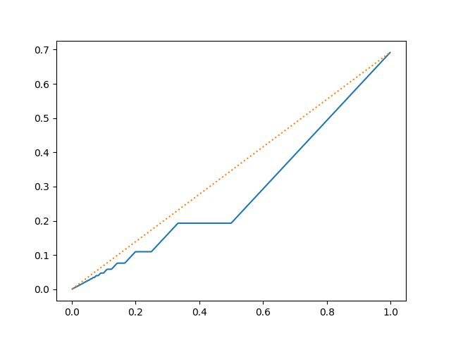
Figure 4. Graph of limit function $f_{BC}(\alpha)$ in $(\alpha,\beta)$-plane, $0\leq\alpha\leq 1.$ The dotted line is $\beta=(\log 2)\alpha$.

The value $\alpha=\frac{1}{2}$ is especially interesting. It concerns $G(2n,n)$ and here Kummer’s criterion gives

$$\frac{G_{BC}(2n,2n)}{G_{BC}(2n,n)}=\prod_{n<p\leq 2n}p.$$ (5.5)

It is well known that the Riemann hypothesis is equivalent to the assertion that for all integers $n\geq 2$,

$$P(n):=\prod_{p\leq n}p=e^{n+O(n^{1/2}(\log n)^{2})}.$$ (5.6)

(Taking logarithms of (5.6), $\log P(n)$ becomes Chebyshev’s first function $\vartheta(n)$ and the equivalence follows from Lemma 2.7 (2).) In consequence one can deduce that the Riemann hypothesis is also equivalent to the assertion that for all $n\geq 2$ ,

$$\frac{P(2n)}{P(n)}=\prod_{n<p\leq 2n}p=e^{n+O(n^{1/2}(\log n)^{2})}.$$ (5.7)

We conclude that the Riemann hypothesis is equivalent to the assertion that for all $n\geq 2$, the partial factorization $G(2n,x)$ with $x=n$ has

$$G_{BC}(2n,n)=G_{BC}(2n,2n)\cdot\frac{P(n)}{P(2n)}=\left(\frac{4}{e}\right)^{n+O(n^{1/2}(\log n)^{2}))}.$$ (5.8)

Taking logarithms in (5.8), we find that the Riemann hypothesis is equivalent to the assertion that at $\alpha=\frac{1}{2}$, for all $n\geq 2$

$$\log G_{BC}(2n,n)=2f_{BC}\left(\,\frac{1}{2}\,\right)n+O\large(n^{1/2}(\log n)^{2}\large),$$ (5.9)

with $f_{BC}(\frac{1}{2})=\log 2-\frac{1}{2}\approx 0.19314$. Thus the Riemann hypothesis is encoded in a power-savings error term $O(n^{1/2}(\log n)^{2})$ in (5.9) at the single point $\alpha=1/2$.

The role the Riemann hypothesis plays in these estimates concerns the rapidity of convergence of the finite $n$ approximations to these limit functions, and not in the particular form of the limit function. The central binomial coefficient exhibits a situation where suitable power savings estimate at a single point $\alpha=\frac{1}{2}$ is equivalent the Riemann hypothesis.

It may be that the power savings estimates given under RH for binomial products in this paper for $0<\alpha<1$ should imply a zero-free region for the Riemann zeta function of form $Re(s)>1-\delta$ for some $\delta>0$. We do not know whether a power-savings estimate at $\alpha=\frac{1}{2}$ alone would imply a zero-free region.

This paper started from an expression for $G(n,n)$ as a ratio of factorials, which led to a power savings estimate at $\alpha=1$. The graph of the limit function $f_{G}(\alpha)$ suggests that the values $x=\frac{n}{j}$ might have special properties, since they lie on the line $y=\frac{1}{2}x.$ One may ask whether factorial product formulas exist for values $G(jn,n)$ when $j\geq 2$.

Appendix A Estimates for $A(n,x)$, $B(n,x)$ and $\log G(n,x)$ via exponential sums

The following result was communicated to us by Olivier Bordellès. One can obtain alternate unconditional bounds for $B(n,x)$ by methods of exponential sums, having a main term involving the first Chebyshev function $\vartheta(x)$, which have nontrivial unconditional remainder terms in various ranges where $x=o(n)$. In this Appendix $B_{1}(x)=x-\frac{1}{2}$ denotes the first Bernoulli polynomial.

Theorem A.1.

For $n\geq 1$ an integer and $1\leq x\leq n$ be a real number, set

$$B(n,x)=\frac{1}{2}\vartheta(x)n+{\widetilde{R}}_{B}(n,x)$$ (A.1)

where $\vartheta(x)$ is the first Chebyshev function and ${\widetilde{R}}_{B}(n,x)$ is the remainder. Then for $n^{2/3}\leq x\leq n$,

$${\widetilde{R}}_{B}(n,x)=O\left(x^{5/4}n^{3/4}(\log n)^{7/2}+n^{5/3}\log n\right).$$ (A.2)

Proof.

Using Lemma 2.1 and $\lfloor x\rfloor=x-\{x\}$, we have

$$B(n,x) = (n-1)\sum_{n^{1/2}<p\leq x}\frac{\log p}{p-1}\left(n-(p-1)\lfloor\frac{n}{p}\rfloor\right)+O\left(n^{3/2}\right)$$

$$= n(n-1)\sum_{n^{1/2}<p\leq x}\frac{\log p}{p-1}-(n-1)\sum_{n^{1/2}<p\leq x}\lfloor\frac{n}{p}\rfloor\log p+O\left(n^{3/2}\right)$$

$$= \left(n(n-1)\sum_{n^{1/2}<p\leq x}\frac{\log p}{p}+n(n-1)\sum_{n^{1/2}<p\leq x}\frac{\log p}{p(p-1)}\right)$$

$$+\left(-n(n-1)\sum_{n^{1/2}<p\leq x}\frac{\log p}{p}+(n-1)\sum_{n^{1/2}<p\leq x}\{\frac{n}{p}\}\log p\right)+O\left(n^{3/2}\right)$$

$$= n(n-1)\sum_{n^{1/2}<p\leq x}\frac{\log p}{p(p-1)}+(n-1)\sum_{n^{1/2}<p\leq x}\{\frac{n}{p}\}\log p+O\left(n^{3/2}\right).$$

The first Bernoulli polynomial has $B_{1}(\{\frac{n}{p}\})=\{\frac{n}{p}\}-\frac{1}{2}$, whence

$$B(n,x) = n(n-1)\sum_{n^{1/2}<p\leq x}\frac{\log p}{p(p-1)}+(n-1)\sum_{n^{1/2}<p\leq x}B_{1}(\{\frac{n}{p}\})\log p$$

$$+\frac{n-1}{2}\left(\vartheta(x)-\vartheta(n^{1/2})\right)+O\left(n^{3/2}\right),$$

$$= \frac{1}{2}\vartheta(x)n+(n-1)\sum_{n^{1/2}<p\leq x}B_{1}(\{\frac{n}{p}\})\log p+O\left(n^{3/2}\log n\right).$$

We obtain

$$B(n,x)=\frac{1}{2}\vartheta(x)n+(n-1)\sum_{n^{1/2}<m\leq x}\Lambda(m)B_{1}(\{\frac{n}{m}\})+O\left(n^{3/2}\log n\right),$$ (A.3)

by inserting $O\left(\frac{n^{1/2}}{\log n}\right)$ extra nonzero terms $\Lambda(m)$ inside the sum, each of size $O(\log n)$.

We estimate the sum containing the von Mangoldt function. If $x\leq 2n^{2/3}$ then

$$|\sum_{n^{1/2}<m\leq x}\Lambda(m)B_{1}(\{\frac{n}{m}\})|\leq|\sum_{n^{1/2}<m\leq 2n^{2/3}}\Lambda(m)|\ll n^{2/3},$$

which gives (A.2) with remainder term ${\widetilde{R}}_{B}(n,x)=O(n^{5/3})$. For $2n^{2/3}\leq x\leq n$, we have

$$|\sum_{n^{1/2}<m\leq x}\Lambda(m)B_{1}(\{\frac{n}{m}\})| \leq |\sum_{n^{1/2}<m\leq 2n^{2/3}}\Lambda(m)B_{1}(\{\frac{n}{m}\})|+|\sum_{2n^{2/3}<m\leq x}\Lambda(m)B_{1}(\{\frac{n}{m}\})\,|$$ (A.4)

$$\ll n^{2/3}+\log n\left(\max_{2n^{2/3}<M\leq x}|\sum_{M<m\leq\min(2M,x)}\Lambda(m)B_{1}(\{\frac{n}{m}\})\,|\right),$$

We use the following estimate, cf. Graham and Kolesnik [17, Theorem A6]. For each integer $H\geq 1$ and for $2n^{2/3}<M\leq n$,

$$|\sum_{M<m\leq\min(2M,x)}\Lambda(m)B_{1}(\{\frac{n}{m}\})|\ll\frac{1}{H}\left(\sum_{M<m\leq 2M}\Lambda(m)\right)+\sum_{h=1}^{H}\frac{1}{h}|\sum_{M<m\leq\min(2M,x)}\Lambda(m)\exp(\frac{2\pi ihn}{m})\,|,$$ (A.5)

with the implied constant in $\ll$ being independent of $H$. (It is based on trigonometric polynomial majorants and minorants to the sawtooth function $B_{1}(\{x\})$.) We apply an exponential sum estimate of Granville and Ramarè [19, Theorem 9’, p.77], which says: For $2n^{2/3}\leq M\leq n$, and any $y^{\prime}$ with $M\leq y^{\prime}\leq 2M$,

$$|\,\sum_{M<m\leq y^{\prime}}\Lambda(m)\exp(\frac{2\pi in}{m})\,|\leq 5M(\frac{M}{n})^{1/4}(\log 16M)^{5/2}.$$

Substituting this bound in (A.5) (with $n$ replaced by $hn$ as needed) yields for any integer $H\geq 1$ such that $2(Hn)^{2/3}\leq M\leq x$,

$$|\sum_{M<m\leq\min(2M,x)}\Lambda(m)B_{1}(\{\frac{n}{m}\})\,| \ll \frac{M}{H}+\sum_{h=1}^{H}\frac{1}{h}\frac{M^{5/4}}{(hn)^{1/4}}(\log M)^{5/2}$$

$$\ll \frac{M}{H}+n^{-1/4}M^{5/4}(\log M)^{5/2}$$

$$\ll nM^{-1/2}+n^{-1/4}M^{5/4}(\log M)^{5/2},$$

where to get the last line we choose $H=\lfloor\frac{1}{2}M^{3/2}n^{-1}\rfloor$. Substituting these bounds into (A.4), noting that $2n^{2/3}\leq M\leq x$, we obtain for $2n^{2/3}\leq x\leq n$,

$$|\sum_{n^{1/2}<m\leq x}\Lambda(m)B_{1}(\{\frac{n}{m}\})|=O\left(x^{5/4}n^{-1/4}(\log n)^{7/2}+n^{2/3}\log n\right).$$

Substituting this estimate in (A.3) gives the desired bound for ${\widetilde{R}}_{B}(n,x)$. ∎

Following the combinatorial approach in this paper, one can deduce from Theorem A.1 the following estimate for $A(n,x)$.

Theorem A.2.

For $n\geq 1$ an integer and $1\leq x\leq n$ a real number, set

$$A(n,x)=\vartheta(x)n+{\widetilde{R}}_{A}(n,x)$$ (A.6)

where $\vartheta(x)$ is the first Chebyshev function and ${\widetilde{R}}_{A}(n,x)$ is the remainder. Then for $n^{2/3}\leq x\leq n$,

$${\widetilde{R}}_{A}(n,x)=O\left(x^{5/4}n^{3/4}(\log n)^{7/2}+n^{5/3}(\log n)^{2}\right).$$ (A.7)

Proof.

We use the combinatorial identity

$$A(n,x)=A(x,x)+\sum_{y=x+1}^{n}\frac{2}{y-1}B(y,x).$$

We have the trivial estimate $A(x,x)\leq A^{\ast}(x,x)=x^{2}.$ Taking $n^{2/3}<x\leq n$ and using the estimate of Theorem A.1, we have

$$A(n,x) = O(x^{2})+\sum_{y=x+1}^{n}\frac{2}{y-1}(\frac{1}{2}\vartheta(x)y)+O\left(\sum_{y=x+1}^{n}\frac{2}{y-1}(x^{5/4}y^{5/4}(\log y)^{7/2}+n^{5/3}\log n)\right)$$

$$= \vartheta(x)(n-x)+O\left(\sum_{y=x+1}^{n}\frac{1}{y}\vartheta(x)\right)+O\left(x^{5/4}\sum_{y=x+1}^{n}y^{-1/4}(\log y)^{7/2}\right)+O\left(n^{5/3}(\log n)^{2}\right)$$

$$= \vartheta(x)n+O\left(x^{2}+x\log n+x^{5/4}n^{3/4}(\log n)^{7/2}+n^{5/3}(\log n)^{2}\right)$$

$$= \vartheta(x)n+O\left(x^{5/4}n^{3/4}(\log n)^{7/2}+n^{5/3}(\log n)^{2}\right),$$

where the last line takes the largest of the terms in the given range of $x$. ∎

Corollary A.3.

For $n\geq 1$ and $1\leq x\leq n$, set

$$\log G(n,x)=\frac{1}{2}\vartheta(x)n+{\widetilde{R}}_{G}(n,x)$$ (A.8)

where $\vartheta(x)$ is the first Chebyshev function and ${\widetilde{R}}_{G}(n,x)$ is the remainder. Then for $n^{2/3}\leq x\leq n$,

$${\widetilde{R}}_{G}(n,x)=O\left(x^{5/4}n^{3/4}(\log n)^{7/2}+n^{5/3}(\log n)^{2}\right).$$ (A.9)

Proof.

Use the identity $\log G(n,x)=A(n,x)-B(n,x)$ together with the estimates in Theorem A.1 and Theorem A.2, noting ${\widetilde{R}}_{G}(n,x)={\widetilde{R}}_{A}(n,x)-{\widetilde{R}}_{B}(n,x)$. ∎

Remark A.4.

The estimates above have a nontrivial error term for $x>n^{2/3}(\log n)^{2+\epsilon}.$ O. Bordellès also observes that one can obtain results parallel to the Theorems above, covering the range $n^{1/2}<x\leq n^{2/3}$ having the same main terms and nontrivial using an exponential sum estimate given in Ma and Wu [28, Proposition 3.1].

References

- [1] R. Bellman and H. N. Shapiro, A problem in additive number theory, Annals of Math. 49 (1948), 333-340.
- [2] L. E. Bush, An asymptotic formula for the average sums of digits of integers, Amer. Math. Monthly 47 (1940), 154–156.
- [3] P. L. Chebyshev, Memoire sur les nombres premiers, J. Maths. Pures Appl. 1852, 17 366–390. [pp. 51–70 in: A. Markoff, N. Sonin, Editors, Oeuvres de P. L. Tschebychef, Tome I, St. Petersburg 1899.]
- [4] L. H. Y. Chen, H-K Hwang, and V. Zacharovas, Distribution of the sum of digits function of random integers: a survey, Prob. Surveys 11 (2014), 177-236.
- [5] H. Delange, Sur la fonction sommatoire de la fonction Somme des chiffres . L’Enseign. Math. 21 (1975), no. 1, 31–47.
- [6] H. Diamond, Elementary methods in the study of the distribution of prime numbers, Bull. Amer. Math. Soc. (N.S.) 7 (1982), no. 3, 553–589.
- [7] H. Diamond and P. Erdős, On sharp elementary prime number estimates, Enseign. Math. 26 (1980), no. 3-4, 313–321.
- [8] H. Diamond and J. Steinig, An elementary proof of the prime number theorem with a remainder term, Invent. Math. 11 (1970), 199–258.
- [9] M. P. Drazin and J. S. Griffith, On the decimal representation of integers, Proc. Camb. Phil. Soc. 48 (1952), 555–565.
- [10] M. Drmota and P. J. Grabner, Analysis of digital functions and applications, pp. 452–504 in: Combinatorics, automata and number theory, Encyclopedia Math. Appl. No. 135. Cambridge University Press, Cambridge 2010.
- [11] L. Du, PhD thesis, University of Michigan, 2020.
- [12] P. Erdős, Bewies eines Satzes von Tschebischeff, Acta. Litt. Sci. Szeged Sect. Math. 5 (1930/1932), 194–198.
- [13] P. Erdős, R. L. Graham, I. Z. Rusza, E. G. Straus, On the prime factors of , Collection of articles in honor of Derrick Henry Lehmer on the occasion of his seventieth birthday, Math. Comp 29 (1975), 83–92.
- [14] P. Erdős, Some of my favorite problems and results, pp. 47–67 in: The Mathematics of Paul Erdős (R. L. Graham and J. Neseteril, Eds.), Springer-Verlag, Berlin/New York 1997.
- [15] P. Flajolet, P. Grabner, P. Kirschenhofer, H. Prodinger and R. F. Tichy, Mellin transforms and asymptotics: digital sums. Theor. Comp. Sci. 123 (1994), 291–314.
- [16] P. J. Grabner and Hsien-Kuei Hwang, Digital sums and divide-and-conquer recurrences: Fourier expansions and absolute convergence, Const. Approx. 21 (2005), 149–179.
- [17] S. W. Graham and G. Kolesnik, Van der Corput’s Method of Exponential Sums, Cambridge Univ. Press 1991.
- [18] A. Granville, Arithmetic properties of binomial coefficients. I. Binomial coefficients modulo prime powers. in: Organic mathematics (Burnaby, BC, 1995), 253–276, CMS Conf. Proc. 20, Amer. Math. Soc. : Providence, RI 1997.
- [19] A. Granville and O. Ramaré, Explicit bounds on exponential sums and the scarcity of squarefree binomial coefficients, Mathematika 43 (1996), 73–107.
- [20] G. H. Hardy, and E. M. Wright, An Introduction to the Theory of Numbers (Fifth Edition). Oxford University Press: Oxford 1979.
- [21] H. Hasse, Number Theory. Translated by H. G. Zimmer from the 1967 German edition. Grundlehren der mathematischen Wissenschaften 229. Springer-Verlag: Berlin-Heidelberg-New York 1980. (Reprinted in series: Classics in mathematics. Springer-Verlag: Berlin 2002.)
- [22] A. E. Ingham, Some Tauberian theorems connected with the prime number theorem, J. London Math. Soc. 22 (1945), 161–180.
- [23] J. C. Lagarias, Euler’s constant: Euler’s work and modern developments. Bull. Amer. Math. Soc. (N. S.) 50 (2013), no. 4, 527–628.
- [24] J. C. Lagarias and H. Mehta, Products of binomial coefficients and unreduced Farey fractions. International Journal of Number Theory, 12 (2016), no. 1, 57-91.
- [25] J. C. Lagarias and H. Mehta, Products of Farey fractions. Experimental Math. 26 ( 2017) no. 1, 1–21.
- [26] A. F. Lavrik and S. S. Sobirov, The remainder term in the elementary proof of the prime number theorem (Russian), Dokl. Akad. Nauk. SSSR 211 (1973), 534–536.
- [27] N. Levinson, The prime number theorem from , Proc. Amer. Math. Soc. bf 15 (1964), 480–485.
- [28] J. Ma and J. Wu, On a sum involving the Mangoldt function, Periodica Math. Hung., to appear.
- [29] L. Mirsky, A theorem on representations of integers in the scale of , Scripta Mathematica 15 (1949), 11–12.
- [30] H. L Montgomery and R. C. Vaughan, Multiplicative Number Theory I. Classical Theory, Cambridge University Press, Cambridge 2007.
- [31] C. Pomerance, Divisors of the middle binomial coefficient, Amer. Math. Monthly 122 (2015) 636–644.
- [32] J. B. Rosser and L. Schönfeld, Approximate formulas for some functions of prime numbers, Illinois J. Math. 6 (1962), 64-94
- [33] I. Rusza, Erdős and the integers, J. Number Theory 79 (1999), 115–163.
- [34] L. Schoenfeld, Sharper bounds for the Chebyshev functions and . II, Math. Comp. 30 (1976), 337–360.
- [35] G. Tenenbaum, Introduction to Analytic and Probabilistic Number Theory, Third Edition, American Math. Soc., Providence, RI 2015.
- [36] J. R. Trollope, An explicit expression for binary digital sums. Math. Mag. 41 (1968), 21–25.