The Toeplitz matrix $e^{-\kappa|i-j|}$ and its application to a layered electron gas

Abstract

We present an explicit solution of the eigen-spectrum of the Toeplitz matrix $C_{ij}=e^{-\kappa|i-j|}$ with $0\leq i,j\leq N,$ and extend it to a combination of a Toeplitz matrix and a Hankel matrix. The solution is found by elementary means that bypass the Wiener-Hopf technique usually used for this class of problems. It rests on the observation that the inverse of $C_{ij}$ is effectively a nearest neighbor hopping model with specific onsite energies, which can in turn be diagonalized easily. We apply this result to find analytically the plasma modes of a layered assembly of 2-dimensional electron gas. We find a sum rule relating the geometric mean of the frequencies of the plasma modes to the determinant of this Toeplitz matrix.

§Introduction:

In the course of our study of layered electronic systems initiated in[1], we came across an interesting Toeplitz matrix

$$C_{ij}=e^{-\kappa|i-j|},\;\hskip 14.45377pt0\leq i,j\leq N.$$ (1)

Eigenfunctions and eigenvalues of Toeplitz matrices are usually found by the Wiener-Hopf technique[2, 3]. The special case of Eq.(1) is called a Kac-Murdock-Szego matrix[4], which can be solved[5, 6, 7, 8] by noting that its inverse is a simple tridiagonal matrix, whose eigenfunctions and eigenvalues can easily be found. An aspect of interest is that the inverse matrix is a tridiagonal matrix, i.e. a nearest neighbor hopping model with a specific on-site and boundary energy. This type of matrix arises in a large number of problems in condensed matter physics, and therefore the relationships found here may thus be of broad interest.

The method of finding the eigenfunctions and eigenvalues of the matrix $C_{ij}$ by constructing its inverse can be generalized to a matrix that is the combination of a Hankel matrix and a Toeplitz matrix:

$$M_{ij}=ae^{-\kappa|i-j|}+be^{\kappa|i-j|}+c\left[e^{-\kappa(i+j)}+e^{-\kappa(2N-i-j)}\right]$$ (2)

with arbitrary $a,b$ and $c.$ This generalization is the subject of this paper.

The particular combination of Hankel and Toeplitz matrices given above is appropriate for solving the plasma modes of a layered assembly of 2-dimensional electron gas. The plasma mode frequencies have been found numerically for this system by a method different from ours[9, 10, 11], and has in fact been studied experimentally using Raman scattering[12]. Applying our method to this problem yields a simple expression for the eigenfunctions associated with these plasma modes, as well as a sum rule relating the frequencies of the (N+1) branches of the plasma frequency as functions of the parallel component of the photon wave vector. The density of states of eigenvalues is also of interest experimentally[14] and evaluated analytically here.

In the rest of this paper, we first review the details of the inversion of C, and two matrices closely related to it, followed by a calculation of the eigenspectrum. We then generalize the method to calculate the eigenspectrum of the matrix $M$ in Eq.(2). Finally, we apply the result to the layered electron gas.

§The Inversion of $C_{ij}$

For $0\leq j\leq N$ we denote the basis column vector $\hat{e}_{j}$ (with1 at the $j^{th}$ row and 0 elsewhere) as $|j\rangle$, and write an operator $\widehat{C}$ such that $\widehat{C}|j\rangle=\sum_{l=0}^{N}C_{lj}|l\rangle$. Let us also denote $\omega_{0}=e^{\kappa}$. We decompose $\widehat{C}$ into right ($\widehat{R}$) and left ($\widehat{L}$) moving parts as

$$\widehat{C}+{\bf 1}=\widehat{R}+\widehat{L},$$ (3)

where ${\bf 1}$ is the identity operator. The operators $\widehat{R}$ and $\widehat{L}$ are defined by their action on the basis states

$$\widehat{R}|j\rangle=\sum_{l=j}^{N}e^{-\kappa(l-j)}|l\rangle=|r_{j}\rangle\equiv\sum_{l=j}^{N}\frac{\omega_{0}^{j}}{\omega_{0}^{l}}\;\;|l\rangle$$ (4)

$$\widehat{L}|j\rangle=\sum_{l=0}^{j}e^{-\kappa(j-l)}|l\rangle=|l_{j}\rangle\equiv\sum_{l=0}^{j}\frac{\omega_{0}^{l}}{\omega_{0}^{j}}\;\;|l\rangle.$$ (5)

Note that the boundary vectors are given by

$$|l_{0}\rangle=|0\rangle,\mbox{ and}\;\;|r_{N}\rangle=|N\rangle.$$ (6)

For the next steps it is useful to note four recursion relations between the basis vectors and their domains

$$|l_{j+1}\rangle=\frac{1}{\omega_{0}}|l_{j}\rangle+|j+1\rangle,\;\;\mbox{for}\;\;0\leq j\leq N-1$$ (7)

$$|l_{j-1}\rangle={\omega_{0}}|l_{j}\rangle-\omega_{0}|j\rangle,\;\;\;\;\mbox{for}\;\;1\leq j\leq N$$ (8)

$$|r_{j+1}\rangle=\omega_{0}|r_{j}\rangle-\omega_{0}|j\rangle,\;\;\;\;\mbox{for}\;\;0\leq j\leq N-1$$ (9)

$$|r_{j-1}\rangle=|j-1\rangle+\frac{1}{\omega_{0}}|r_{j}\rangle\;\;\;\;\mbox{for}\;\;1\leq j\leq N.$$ (10)

Let us calculate the action of $\widehat{C}$ on the states. Consider first the interior terms $1\leq j\leq N-1$:

$$(\widehat{C}+{\bf 1})|j+1\rangle = |r_{j+1}\rangle+|l_{j+1}\rangle$$ (11)

$$= \omega_{0}|r_{j}\rangle+\frac{1}{\omega_{0}}|l_{j}\rangle+|j+1\rangle-\omega_{0}|j\rangle,$$

using Eqs. (7,9). Similarly

$$(\widehat{C}+{\bf 1})|j-1\rangle = |r_{j-1}\rangle+|l_{j-1}\rangle$$ (12)

$$= \frac{1}{\omega_{0}}|r_{j}\rangle+\omega_{0}|l_{j}\rangle-\omega_{0}|j\rangle+|j-1\rangle$$

using Eqs. (8,10). Adding Eq. (11) and Eq. (12) and rearranging we find

$$\widehat{C}(|j+1\rangle+|j-1\rangle)=(\omega_{0}+\frac{1}{\omega_{0}})\widehat{C}|j\rangle-(\omega_{0}-\frac{1}{\omega_{0}})|j\rangle.$$ (13)

Multiplying through by the inverse operator $\widehat{C}^{-1}$ we find

$$\widehat{C}^{-1}|j\rangle=\coth{\kappa}|j\rangle-\frac{1}{2\sinh{\kappa}}(|j+1\rangle+|j-1\rangle).$$ (14)

To determine the action of $\widehat{C}^{-1}$ on the boundary term $j=0$ we note

$$({\bf 1}+\widehat{C})|1\rangle = |l_{1}\rangle+|r_{1}\rangle=|1\rangle+\frac{1}{\omega_{0}}|0\rangle+\omega_{0}|r_{0}\rangle-\omega_{0}|0\rangle,$$

$$\widehat{C}|1\rangle = \omega_{0}|r_{0}\rangle-(\omega_{0}-\frac{1}{\omega_{0}})|0\rangle$$ (15)

where we used Eq. (6), Eq. (7) and Eq. (9). Now observe that on using Eq. (6)

$$\widehat{C}|0\rangle=|r_{0}\rangle,$$ (16)

and hence we may write

$$\widehat{C}|1\rangle=\omega_{0}\widehat{C}|0\rangle-(\omega_{0}-\frac{1}{\omega_{0}})|0\rangle,$$ (17)

or taking the inverse,

$$\widehat{C}^{-1}|0\rangle=\frac{e^{\kappa}}{2\sinh{\kappa}}|0\rangle-\frac{1}{2\sinh{\kappa}}|1\rangle.$$ (18)

To determine the action of $\widehat{C}^{-1}$ on the boundary term $j=N$ we note that

$$\widehat{C}|N-1\rangle = \omega_{0}|l_{N}\rangle-\omega_{0}|N\rangle+\frac{1}{\omega_{0}}|N\rangle$$ (19)

where Eq. (6) and Eq. (10) have been used. We further use

$$\widehat{C}|N\rangle=|l_{N}\rangle,$$ (20)

so that

$$\widehat{C}|N-1\rangle = \omega_{0}\widehat{C}|N\rangle-\omega_{0}|N\rangle+\frac{1}{\omega_{0}}|N\rangle.$$ (21)

Upon inversion we get

$$\widehat{C}^{-1}|N\rangle=\frac{e^{\kappa}}{2\sinh{\kappa}}|N\rangle-\frac{1}{2\sinh{\kappa}}|N-1\rangle.$$ (22)

Combining Eq. (18), Eq. (22) and Eq. (14) we write the inverse matrix in the form of a tight-binding Hamiltonian

$$\widehat{C}^{-1}=\sum_{j=0}^{N}\varepsilon(j)|j\rangle\langle j|-\tau\sum_{j=0}^{N-1}\left\{|j\rangle\langle j+1|+|j+1\rangle\langle j|\right\},$$

$$\tau=\frac{1}{2\sinh{\kappa}}$$

$$\varepsilon(1)=\varepsilon(2)=\cdots=\varepsilon(N-1)=\coth{\kappa},$$

$$\varepsilon(0)=\varepsilon(N)=\frac{e^{\kappa}}{2\sinh{\kappa}};\;\;$$ (23)

§Inverses of $\widehat{R}$ and $\widehat{L}$

It is interesting to note the inverses

$$\widehat{R}^{-1}={\bf 1}-e^{-\kappa}\sum_{j=0}^{N-1}|j+1\rangle\langle j|$$ (24)

i.e. the identity minus a right shift operator, and

$$\widehat{L}^{-1}={\bf 1}-e^{-\kappa}\sum_{j=0}^{N-1}|j\rangle\langle j+1|$$ (25)

i.e. the identity minus a left shift operator. The proof uses a similar idea as before. For Eq. (24) with $0\leq j\leq N-1$, we use Eq. (9) to write

$$\widehat{R}|j+1\rangle=\omega_{0}\widehat{R}|j\rangle-\omega_{0}|j\rangle,\;\mbox{or}\;\;\widehat{R}^{-1}|j\rangle=|j\rangle-\frac{1}{\omega_{0}}|j+1\rangle,$$ (26)

and for the boundary term use $\widehat{R}^{-1}|N\rangle=|N\rangle$. For Eq. (25) with $0\leq j\leq N-1$, we use Eq. (7) to write

$$\widehat{L}|j+1\rangle=\frac{1}{\omega_{0}}\widehat{L}|j\rangle+|j+1\rangle,\;\;\mbox{or}\;\;\widehat{L}^{-1}|j+1\rangle=|j+1\rangle-\frac{1}{\omega_{0}}|j\rangle,$$ (27)

and for the boundary term $\widehat{L}^{-1}|0\rangle=|0\rangle$. Together these result in Eq. (24) and Eq. (25).

§Diagonalizing of $\widehat{C}$

It is actually easier to diagonalize $\widehat{C}^{-1}$ in Eq. (23). We try the wave function

$$|\Psi(q)\rangle=\sum_{j=0}^{N}\cos(qj-\Phi(q))|j\rangle$$ (28)

such that

$$\widehat{C}^{-1}|\Psi(q)\rangle=\Lambda^{-1}|\Psi(q)\rangle.$$ (29)

Here $q$ and $\Phi(q)$ as well as the eigenvalue $\Lambda$ are to be determined. The interior terms $1\leq j\leq N-1$ are satisfied by this wavefunction provided

$$\Lambda^{-1}=\coth\kappa-\frac{\cos q}{\sinh\kappa},$$ (30)

and the amplitude at $j=0$ requires the condition

$$(\Lambda^{-1}-\varepsilon(0))\cos\Phi=-\tau\cos(q-\Phi),$$ (31)

or simplifying further we find the phase shift determined by

$$\Phi(q)=\mbox{arccot}\left\{\frac{\sin q}{\cos q-e^{-\kappa}}\right\}.$$ (32)

The phase shift $\Phi(q)$ varies continuously with $q$ in the interval $0\leq q\leq\pi$, decreasing monotonically from $\pi/2$ to $-\pi/2$. It is thus a convenient parameterization for finding all the eigenvalues. The amplitude at $j=N$ is satisfied if

$$(\Lambda^{-1}-\varepsilon(N))\cos(qN-\Phi(q))=-\tau\cos(q(N-1)-\Phi(q)),$$ (33)

or simplifying further

$$\sin(qN-2\Phi(q)) = 0.$$ (34)

Alternatively, we can observe that the eigenfunctions must be odd or even functions of the index $j$ measured from the midpoint of $j=N/2$ (this is true even if $N$ is odd), so that either $\sin(qN/2-\Phi(q))$ or $\cos(qN/2-\Phi(q))$ is zero for each eigenfunction. The product of the two expressions, and therefore $\sin(qN-2\Phi(q))$ must therefore be zero for every eigenfunction. It is straightforward to verify that the N values $\nu=0,1,\ldots N$ yield the $N+1$ distinct eigenvalues

$$\Lambda(q_{\nu},\kappa) = \frac{\sinh\kappa}{\cosh\kappa-\cos q_{\nu}},\;\;\mbox{with}$$ (35)

$$q_{\nu}N = \nu\pi+2\Phi(q_{\nu}).$$ (36)

We will usually denote $\Lambda(q_{\nu},\kappa)$ as $\Lambda(q_{\nu})$. At finite $N$ the values $q=0$ and $q=\pi$ are excluded since for these the wavefunction $|\Psi(q)\rangle$ vanishes identically, formally these correspond to $\nu=-1$ and $\nu=N+1$ respectively. Also we note that in the limit $\kappa\to+\infty$, the phase shift $\Phi(q)=\pi/2-q$ and hence $q_{\nu}=\frac{\nu+1}{N+2}\pi$.

The matrices $\widehat{R}$ and $\widehat{L}$ act as raising or lowering operators and do not have the usual eigenfunctions, however it is easy to construct their generalized eigenfunctions.

§Density of states

For large N it is useful to employ the density of states of the exact eigenvalues, these can be found straightforwardly. We note the identity

$$\frac{d\Phi(q)}{dq}=-\frac{1}{2}(1+\Lambda(q)),$$ (37)

so that we can write the difference in successive solutions from Eq. (36) in the form

$$\pi\Delta\nu=N\Delta q_{\nu}-2\Delta\Phi(q_{\nu})=\Delta q_{\nu}(N+1+\Lambda(q_{\nu}))$$ (38)

so that

$$\sum_{\nu=0}^{N}\to\int_{q_{0}}^{q_{N}}\frac{dq}{\pi}\left\{N+1+\Lambda(q)\right\}.$$ (39)

From Eq. (36)

$$\frac{dq}{d\Lambda}=-\frac{\sinh\kappa}{\Lambda^{2}\left[1-(\cosh\kappa-\frac{\sinh\kappa}{\Lambda})^{2}\right]^{\frac{1}{2}}}$$ (40)

and hence we can convert a sum over solutions to an integral over eigenvalues with a density of states

$$\sum_{\nu}\to\frac{1}{\pi}\int_{\Lambda_{<}}^{\Lambda_{>}}\frac{d\Lambda}{\Lambda^{2}}\frac{\left\{N+1+\Lambda\right\}\sinh\kappa}{\Lambda^{2}\left[1-(\cosh\kappa-\frac{\sinh\kappa}{\Lambda})^{2}\right]^{\frac{1}{2}}}$$ (41)

where

$$\Lambda_{<}=\frac{\sinh\kappa}{\cosh\kappa+1},\;\;\Lambda_{>}=\frac{\sinh\kappa}{\cosh\kappa-1}.$$ (42)

§Szegő’s theorem for the determinant of $C_{ij}$

It is interesting to compute the determinant of $C$. For the matrix Eq. (1) we are in the happy position of being able to do so exactly by using Gauss’s method of triangulation, leading to

$$||C||=det(C)=(1-e^{-2\kappa})^{N}.$$ (43)

The proof is elementary. An alternative approach exploits the tridiagonal nature of $C^{-1}.$ If one defines $A_{j}$ to be the $j\times j$ submatrix of $(2\sinh\kappa)C^{-1}$ that ends at the bottom right corner of $C^{-1},$ it is easy to verify that $||A_{j+1}||=V_{j}||A_{j}||-||A_{j-1}||$ for $j=1,2\ldots N$ with the boundary condition $||A_{0}||=1$ and $||A_{1}||=e^{\kappa},$ and $V_{j}=e^{\kappa}\delta_{j,N}+(1-\delta_{j,N})2\cosh\kappa.$ With the boundary condition, the solution to the recurrence relation is $||A_{j}||=e^{j\kappa}$ for $0\leq j\leq N,$ and so $||A_{N+1}||=e^{(N+1)\kappa}(1-e^{-2\kappa}).$ Therefore $||C||=(2\sinh\kappa)^{N+1}/[e^{(N+1)\kappa}(1-e^{-2\kappa})]=(1-e^{-2\kappa})^{N}.$

We can also calculate the determinant from the strong theorem of Szegő [15], which is guaranteed to give the two leading terms in the limit of large N. Specifically the theorem says that when the (N+1)x(N+1) Toeplitz matrix $C$ is generated by a density $\phi(\theta)$ through a Fourier series, i.e.

$$C(i-j)=\int_{-\pi}^{\pi}\;\frac{d\theta}{2\pi}\;e^{-i\theta(i-j)}\phi(\theta)$$ (44)

and further if

$$\log\phi(\theta)=\sum_{l=-\infty}^{\infty}e^{il\theta}\nu_{l}$$ (45)

then the determinant for large $N$ is given by

$$||C||=\exp\{(N+1)\nu_{0}+\sum_{l=1}^{\infty}l|\nu_{l}|^{2}+o(N)\}.$$ (46)

In the present case of Eq. (1) it is readily seen that

$$\phi(\theta) = \frac{\sinh\kappa}{\cosh\kappa-\cos(\theta)},\;\;\mbox{and}$$ (47)

$$\nu_{l} = \delta_{l,o}\left(\log 2\sinh\kappa-\kappa\right)+(1-\delta_{l,o})\frac{e^{-\kappa|l|}}{|l|}.$$ (48)

Substituting into Eq. (46) and carrying out the summation over $l$ we see that Szegő’s theorem gives

$$||C|| = \exp\{(N+1)\left[\log(1-e^{-2\kappa})\right]-\left[\log(1-e^{-2\kappa})\right]+o(N)\}$$ (49)

$$= \exp\{N\left[\log(1-e^{-2\kappa})\right]+o(N)\}.$$

Comparing with Eq. (43) we see that the above expression is exact if we drop the $o(N)$ correction terms altogether. We can also calculate the determinant using the exact eigenvalues $\Lambda$ given in Eq. (36) and employing the Euler-Mclaurin formula. The first two terms are the same as in Eq. (49). The rather unexpected vanishing of the $o(N)$ correction term, as explained to us by Prof. Ehrhardt, is the consequence of the following general result[16]: define $\varphi(z)=\sum_{k=-\infty}^{\infty}C_{k+j,j}z^{k}.$ If $1/\varphi(z)$ has a Laurent series in which all $\sim z^{k}$ terms vanish for $k>m$ or $k<-m,$ then the determinant of $C$ is of the form $G^{N}E$ for $N+1\geq m,$ for some constants $E$ and $G.$ (The constants can be defined as $G=||C_{N=m}||/||C_{N=m-1}||$ and $E=||C_{N=m}||/G^{m}.$) In the case at hand, $m=1,$ and the determinant grows exponentially with $N$ over the entire range of $N.$

§Generalization to combined Toeplitz Hankel matrices

Toeplitz matrices are closely related to Hankel matrices: the elements $H_{ij}$ of a Hankel matrix $H$ only depend on $i+j.$ It is clear that any Hankel matrix is related to some Toeplitz matrix through reflection about the midpoint: $i\rightarrow N-i$ or $j\rightarrow N-j.$ In particular, the matrix

$$\tilde{H}_{ij}=e^{-\kappa|i+j-N|},\;\hskip 14.45377pt0\leq i,j\leq N.$$ (50)

is a reflection of the Toeplitz matrix $C_{ij}$ which we have analyzed. Since $\tilde{H}=RC,$ where $R$ is the reflection operator, any eigenvector of $C$ satisfies $\tilde{H}|\psi\rangle=RC|\psi\rangle=\lambda R|\psi\rangle.$ Since, as we have remarked earlier, the eigenvectors of $C$ are even or odd under reflection about the midpoint, $\tilde{H}|\psi\rangle=(-1)^{P}\lambda|\psi\rangle,$ where $P$ is the parity of the eigenvector.

A related Hankel matrix, $H_{ij}=\exp[-\kappa(i+j)],$ for which there is no cusp on the diagonal, is even simpler to solve. It is easy to verify that any vector $|\psi\rangle$ that satisfies $\sum_{j}\exp[-j\kappa]\psi_{j}=0$ is a null vector of $H.$ Thus the null space of $H$ is $N$-dimensional, and the $N+1$’th eigenvector must be the vector that is orthogonal to this subspace: $\psi_{j}=\exp[-j\kappa]$ (unnormalized), with eigenvalue $\sum\exp[-2j\kappa].$

We now consider the problem of finding the eigenvalues of a combination of Hankel and Toeplitz matrices:

$$M_{ij}=a\exp\left[-\kappa|i-j|\right]+b\exp\left[\kappa|i-j|\right]+c\left\{\exp\left[-\kappa(i+j)\right]+\exp\left[-\kappa(2N-i-j)\right]\right\}$$ (51)

with the restriction $a\neq b.$ Each of the four parts of this matrix can be solved (in our discussion of the matrix $C,$ there was no restriction that $\kappa$ had to be positive), but they are non-commuting.

We define the tridiagonal matrix $T$

$$T=\frac{1}{2(a-b)\sinh\kappa}\begin{pmatrix}e^{\kappa}&-1&0\ldots\\ -1&2\cosh\kappa&-1\ldots\\ \vdots&&\ddots\end{pmatrix}$$ (52)

which is the same tridiagonal matrix we used earlier, except for the factor of $a-b$ in the denominator. Then it is possible to verify that

$$TM=I+\begin{pmatrix}\alpha_{0}&\alpha_{1}&\ldots\\ 0&0&\ldots\\ \vdots&\vdots&\ddots\\ \alpha_{N}&\alpha_{N-1}&\ldots\end{pmatrix}$$ (53)

i.e. the matrix $T$ is the inverse of $M$ except for boundary effects. Explicitly, the elements of the boundary rows are

$$\alpha_{i}=\frac{1}{a-b}(b\exp[\kappa i]+c\exp[-\kappa i]).$$ (54)

The actual inverse of $M$ is then

$$M^{-1}=T+\begin{pmatrix}x_{0}&x_{1}&\ldots\\ 0&0&\ldots\\ \vdots&\vdots&\ddots\\ x_{N}&x_{N-1}&\ldots\end{pmatrix}$$ (55)

where, taking advantage of the symmetry properties of $M,$ the condition to be satisfied by the $x_{i}$’s is

$$M\begin{pmatrix}x_{0}\\ x_{1}\\ \vdots\\ x_{N}\end{pmatrix}=-\begin{pmatrix}\alpha_{0}\\ \alpha_{1}\\ \vdots\\ \alpha_{N}\end{pmatrix}.$$ (56)

This has the solution

$$\begin{pmatrix}x_{0}\\ x_{1}\\ \vdots\\ x_{N}\end{pmatrix}=-T\begin{pmatrix}\alpha_{0}\\ \alpha_{1}\\ \vdots\\ \alpha_{N}\end{pmatrix}-\begin{pmatrix}\sum\alpha_{i}x_{i}\\ 0\\ \vdots\\ \sum\alpha_{N-i}x_{i}\end{pmatrix}.$$ (57)

Substituting Eq.(54) in the first term on the right hand side, all the elements of $T\cdot\alpha$ except the first and last ones are zero. Therefore, $x_{1},x_{2}\ldots x_{N-1}=0$ and we are left with the coupled equations

$$(a-b)\begin{pmatrix}x_{0}\\ x_{N}\end{pmatrix}=-\frac{1}{a-b}\begin{pmatrix}c\\ be^{N\kappa}\end{pmatrix}-\begin{pmatrix}x_{0}&x_{N}\\ x_{N}&x_{0}\end{pmatrix}\begin{pmatrix}b+c\\ be^{N\kappa}+ce^{-N\kappa}\end{pmatrix}$$ (58)

which has the solution

$$x_{0} = \frac{ac-bc+c^{2}-b^{2}e^{2\kappa N}}{(a-b)[(a+c)^{2}-(ce^{-N\kappa}+be^{N\kappa})^{2}}$$

$$x_{N} = \frac{c^{2}e^{-N\kappa}-abe^{N\kappa}}{(a-b)(a^{2}+2(a-b)c-b^{2}e^{2N\kappa}+c^{2}(1-e^{-2N\kappa})}.$$ (59)

Once we have obtained $M^{-1}$ in the form of Eq.(55), it is easy to see that the eigenvectors can be written with elements $\psi_{q}(j)=\cos[q(j-N/2)]$ or $\psi_{q}(j)=\sin[q(j-N/2)].$ The eigenvalues are related to $q$ through

$$\Lambda^{-1}=\frac{1}{a-b}\left[\coth\kappa-\frac{\cos q}{\sinh\kappa}\right].$$ (60)

The boundary conditions for the even and odd eigenvectors

$$(x_{0}+x_{N})\cos qN/2+\frac{e^{-\kappa}}{2(a-b)\sinh\kappa}[\cos qN/2+\cos q(N/2+1)] = 0$$

$$(x_{0}-x_{N})\sin qN/2+\frac{e^{-\kappa}}{2(a-b)\sinh\kappa}[\sin qN/2+\sin q(N/2+1)] = 0$$

respectively determine the allowed values of $q.$

From Eq.(53), it is easy to see that

$$det(M)=(1+\alpha_{0})^{2}/det(T)=(a-b)^{N-1}(a+c)^{2}((1-e^{-2\kappa})^{N}.$$ (62)

§2-d Plasmon spectrum

As mentioned in the introduction, the Toeplitz matrix $C_{ij}$ arises in the context of plasmons in multilayer systems, a system that has been studied extensively earlier. The original systems studied in the work of Olego, Pinczuk, Gossard and Wiegmann [12, 13] consists of alternating layers of insulating $GaAs$ and conducting $(Al_{x}Ga_{1-x})As$. Here the conducting planes are coupled by the Coulomb interaction only, i.e. one ignores the direct hopping of electrons between layers [1]. Recent advances in materials allows a vast range of composite materials, generalizing this initial system [17, 18, 19, 20]. To understand plasmons in these systems, one needs to understand the dielectric function of layered systems [11, 10, 9], where the plasmon is a pole of a charge response function, probed by either a charged particle surface scattering, or as in the case of [12, 13, 9] by photons using Raman scattering. Within the widely used random phase approximation for these systems, the plasmon is found as the eigen-solution of a homogeneous Fredholm equation[9] satisfied by $\delta\rho(l)$, the induced charge density on layer $l$ due to a small excess external charge:

$$\delta\rho(l)=D_{0}(k_{\small||},\omega)V(k_{\small||})\sum_{m=0}^{N}e^{-k_{\small||}d|l-m|}\delta\rho(m),$$ (63)

where $k_{\small||}$ is the magnitude of the component of the photon parallel to the 2-d layer, d the separation between the $N+1$ layers, $V(k_{\small||})=\frac{2\pi e^{2}}{k_{\small||}\varepsilon_{M}}$ and $\varepsilon_{M}$ is the material dielectric constant. Here $D_{0}(k_{\small||},\omega)$ is the ”bubble” polarization in 2-d; it is approximated well in terms of the 2-d density $n$ and effective mass $m^{*}$ by

$$D_{0}\sim\frac{nk_{\small||}^{2}}{m^{*}\omega^{2}}.$$

When the dielectric constants in the different layers are different, one must also add image charges to Eq. (63) as explained in [9], who provide a complete numerical solution for all cases.

Comparing Eq. (63) with Eq. (1) we see that the plasmon frequencies for the $N+1$ layer problem are obtained from $\Lambda_{\nu}$ in Eq. (35)

$$\omega_{\nu}(k_{\small||})=\sqrt{\frac{2\pi ne^{2}}{\varepsilon_{M}m^{*}}}\sqrt{k_{\small||}\Lambda(q_{\nu},\kappa)}$$ (64)

by identifying $\kappa=k_{\small||}d$. The allowed $q_{\nu}$’s are given by Eq. (36), and are not evenly spaced. The exact determination of the Toeplitz determinant implies that we have a sum-rule on

$$\langle\omega(k_{\small||})\rangle_{gm} \equiv \left[\prod_{\nu=0}^{N}\omega_{\nu}(k_{\small||})\right]^{\frac{1}{N+1}}$$ (65)

$$= \sqrt{\frac{2\pi ne^{2}}{\varepsilon_{M}m^{*}}}\sqrt{k_{\small||}}\left[(1-e^{-2k_{\small||}d})\right]^{\frac{N}{2(N+1)}}$$

In Fig. (1) we illustrate the plasmon solutions for the case of 6 layers using parameters close to those in [12], and also display the geometric mean.

It is useful to note that in general layered systems, the background dielectric function varies between layers , often described as a $\epsilon_{0}$-$\epsilon$-$\epsilon_{0}$ configuration of the layers [9]. The pure Toeplitz spectrum is obtained when $\epsilon_{0}=\epsilon$. In fact the experiment in [13] corresponds to such a case, with a vanishing dielectric contrast.

In the generic $\epsilon_{0}$-$\epsilon$-$\epsilon_{0}$ configuration of the layers [9], the problem corresponds to the more complicated Toeplitz-Hankel combination discussed in the previous section, with (in the notation of Ref. [9], with $N\rightarrow N+1$)

$$c/a = \frac{\epsilon-\epsilon_{0}}{\epsilon+\epsilon_{0}}\exp[-\kappa(L-Nd)]$$

$$b/a = \left(\frac{\epsilon-\epsilon_{0}}{\epsilon+\epsilon_{0}}\right)^{2}\exp[-2\kappa(L/d)].$$ (66)

The right hand side of Eq.(65) is multiplied by

$$[(1-b/a)^{N-1}(1+c/a)^{2}]^{1/(N+1)}(1-b/a)^{-1/2}.$$ (67)

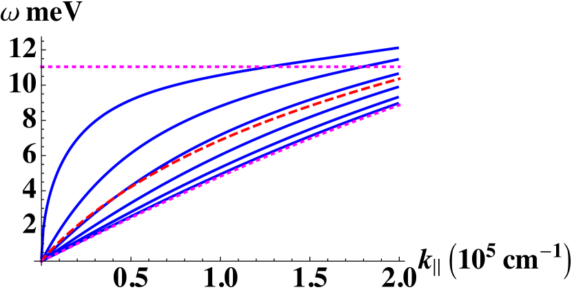
Figure 1: The six plasmon branches for a six layer system in blue solid curves, the geometric mean frequency from Eq. (65) in red dashed curve, and the 3-d bulk and 2-d bulk plasmon in magenta dotted curves. The parameters used are similar to those of sample 1 in [12], we used d= 900$A^{0}$, n=7.3$\times 10^{11}$ cm^-2, $m^{*}=0.07m_{e}$, $\varepsilon=13.1$.

§Acknowledgments:

We thank Professor J. K. Jain and Professor Aaron Pinczuk for a helpful correspondence, and Professor Torsten Ehrhardt for feedback about prior work on Toeplitz matrices. We also thank Professor Peter Forrester for pointing out Ref.[5]. The work at UCSC was supported by the US Department of Energy (DOE), Office of Science, Basic Energy Sciences (BES), under Award No. DE-FG02-06ER46319.

References

[1] P. B. Visscher and L. M. Falicov, Phys. Rev. B3, 2541 (1971).
[2] P. Deift, A. Its and I. Kravosky, arXiv:1207.4990 (2012). This article gives an illuminating account of the impact of Toeplitz matrix theory on exactly solvable models in statistical mechanics, in particular on Lars Onsager’s celebrated solution of the spontaneous magnetization in 2-dimensional Ising model..
[3] A. Caledron, F. Spitzer and H. Widom, Illinois J. Math. 3, 490 (1959).
[4] M. Kac, W.L. Murdock, and G. Szegő, J. Rat. Mech. Anal. 2, 767 (1953).
[5] J.N. Pierce and S. Stein, Proc. IRE 48, 89 (1960).
[6] R.A. Horn and C.R. Johnson, Matrix analysis, Cambridge University Press (Cambridge, 1991).
[7] W.F. Trench, Lin. Alg. Appl. 294, 181 (1999).
[8] A. N. Poddubny, Phys. Rev. A 101,043845 (2020).
[9] Jainendra K. Jain and Philip B. Allen, Phys. Rev. Letts. 54 2437 (1985); Phys. Rev. B32, 997 (1985).
[10] S. Das Sarma and J. J. Quinn, Phys. Rev. B25, 7603 (1982).
[11] A. Fetter, Ann. Phys. (N.Y.) 88, 1 (1974).
[12] D. Olego, A. Pinczuk, A. C. Gossard and W. Wiegmann, Phys. Rev. B25, 7867 (1982).
[13] A. Pinczuk, M. G. Lamont and A. C. Gossard, Phys. Rev. Letts. 56, 2092 (1986).
[14] H. Morawitz, I. Bozovic, V. Z. Kresin, G. Rietveld and D. van der Marel, Z. Phys. B 90, 277 (1993).
[15] G. Szegő On certain hermitian forms associated with the Fourier series of a positive function, Festschrift Marcel Riesz, Lund 228-238 (1952). Also see U. Grenander and G. Szegő, Toeplitz forms and their applications, University of California Press, Berkeley and Los Angeles, 1958.
[16] H. Widom, Adv. Math. 13, 284 (1974).
[17] H.G. Yan, X.S. Li, B. Chandra et al, Nature Nanotech. 7, 330 (2012).
[18] A.M. Da Silva, Y.C. Chang, T. Norris and A.H. MacDonald, Phys. Rev. B 88, 195411 (2013).
[19] V.A. Volodin, M.D. Efremov, V.V. Preobrazhenskii et al, JETP Lett. 71, 477 (2000).
[20] K. Okamoto, D. Tanaka, R. Degawa et al, Sci. Rep. 6, 36165 (2016).