Changes in air quality and human mobility in the U.S. during the COVID-19 pandemic

Abstract

The first goal of this study is to quantify the magnitude and spatial variability of air quality changes in the U.S. during the COVID-19 pandemic. We focus on two pollutants that are federally regulated, nitrogen dioxide (NO2) and fine particulate matter (PM_2.5). NO2 is emitted during fuel combustion by all motor vehicles and airplanes. PM_2.5 is emitted by airplanes and, among motor vehicles, mostly by diesel vehicles, such as commercial heavy-duty diesel trucks. Both PM_2.5 and NO2 are also emitted by conventional power plants, although PM_2.5 almost exclusively by coal power plants. Observed concentrations at all available ground monitoring sites (240 and 480 for NO2 and PM_2.5, respectively) were compared between April 2020, the month during which the majority of U.S. states had introduced some measure of social distancing (e.g., business and school closures, shelter-in-place, quarantine), and April of the prior five years, 2015–2019, as the baseline. Large, statistically-significant decreases in NO2 concentrations were found at more than 65% of the monitoring sites, with an average drop of 2 parts per billion (ppb) when compared to the mean of the previous five years. The same patterns are confirmed by satellite-derived NO2 column totals from NASA OMI, which showed an average drop in 2020 by 13% over the entire country when compared to the mean of the previous five years. PM_2.5 concentrations from the ground monitoring sites, however, were not significantly lower in 2020 than in the past five years and were more likely to be higher than lower in April 2020 when compared to the previous five years.

The second goal of this study is to explain the different responses of these two pollutants, i.e., NO2 was significantly reduced but PM_2.5 was nearly unaffected, during the COVID-19 pandemic. The hypothesis put forward is that the shelter-in-place measures affected people’s driving patterns most dramatically, thus passenger vehicle NO2 emissions were reduced. Commercial vehicles (generally diesel) and electricity demand for all purposes remained relatively unchanged, thus PM_2.5 concentrations did not drop significantly. To establish a correlation between the observed NO2 changes and the extent to which people were actually sheltering in place, thus driving less, we use a mobility index, which was produced and made public by Descartes Labs. This mobility index aggregates cell phone usage at the county level to capture changes in human movement over time. We found a strong correlation between the observed decreases in NO2 concentrations and decreases in human mobility, with over 4 ppb decreases in the monthly average where mobility was reduced to near zero and around 1 ppb decrease where mobility was reduced to 20% of normal or less. By contrast, no discernible pattern was detected between mobility and PM_2.5 concentrations changes, suggesting that decreases in personal-vehicle traffic alone may not be effective at reducing PM_2.5 pollution.

1 Introduction

Worldwide, about 91% of the population is exposed to poor air quality. The World Health Organization (WHO) estimates that on average, 4.2 million people die each year from causes directly attributed to air pollution whodeath . Nitrogen dioxide (NO2) is one of a group of highly reactive gases known as nitrogen oxides (NOx). NO2 can irritate the human respiratory system and is also harmful to ecosystems by the formation of nitric acid and acid rain epano2 ; lin2011 . PM_2.5 is another harmful air pollutant that consists of microscopic particles with a diameter smaller than 2.5 $\mu$m. These particles can pose a great risk to human health because they can penetrate into human lungs and even the bloodstream; PM_2.5 is also often associated with poor visibility epapm . NO2 and PM_2.5 are both primary (i.e., they can be directly emitted into the atmosphere) and secondary (i.e., they can also form after chemical reactions in the atmosphere) pollutants. High concentrations of both are not necessarily found where their emissions are highest, due to processes such as chemical reactions, transport, or diffusion. NO2 and PM_2.5 are the main focus of this paper because they are among the seven “criteria” pollutants that are regulated at the federal level by the U.S. Environmental Protection Agency (EPA) via the National Ambient Air Quality Standards (NAAQS).

The novel coronavirus disease (SARS-CoV-2/COVID-19, COVID-19 hereafter for brevity) was first identified in Wuhan, China, on December 30, 2019 who ; chan2020 . Cases started to spread initially in China but quickly expanded to other countries across the world. COVID-19 was declared a global pandemic in March 2020 whoEurope . At the time of this study, over 9 million people have been affected by the virus, with over 470,000 deaths in 213 countries and territories worldometer ; JHU . COVID-19 first reached the U.S. in February 2020 and since then it has caused over 120,000 deaths in the span of a few months cdc ; JHU . The death rate of COVID-19 is significantly higher among people with cardiovascular and respiratory illnesses acc , which are also strongly connected with air pollution isaifan2020 . Furthermore, new studies suggest that higher concentrations of air pollutants result in a higher risk of COVID-19 infection yongjian2020 and mortality wu2020 .

In the U.S., social distancing measures were implemented state by state with the goal of limiting the spread of the pandemic. In general, closure or non-physical interaction options (e.g., delivery only) were implemented for schools, restaurants, and public places of gathering. Businesses, workers, and types of activities that were deemed essential during the pandemic either continued operating under strict protection measures (e.g., personal protective equipment (PPE), masks) or switched to online work. Non-essential businesses requiring physical presence and interaction closed completely (e.g., hair salons, bars, gyms). The extent of social distancing measures, seriousness of the implementation, and the degree of compliance varied throughout the U.S. Most states announced some level of social distancing orders starting in mid-March, 2020 bbc , often including a mandatory quarantine for people diagnosed with or showing symptoms of the coronavirus. By the beginning of April, almost all states had a mandatory shelter-in-place or lockdown order nystats . Hereafter, lockdown and shelter-in-place will be used interchangeably. The social distancing measures have led to drastic changes in mobility and energy use and therefore changes in emissions of pollutants.

Globally, the COVID-19 outbreak is forcing large changes in economic activities NCAR . In China, following the strict social distancing measures, transportation decreased noticeably and, as a result, China experienced a drastic decrease in atmospheric pollution, specifically CO NCAR , NO2, and PM_2.5 manuel2020 ; NCAR ; nasa concentrations in major urban areas. However, emissions from residential heating and industry remained steady or slightly declined chen2020 . Using satellite data, Zhang et al. zhang2020nox and the National Center for Atmospheric Research NCAR reported a 70% and 50% decrease in NOx concentrations in Eastern China, respectively. Bao and Zhang bao2020 showed an average of 7.8% decrease in the Air Quality Index over 44 cities in northern China. Bawens et al. Bauwensetal2020 and Shi and Brasseur ShiBra20 reported an increase in O3 concentrations in the same region. Chen et al. chen2020 , reported that NO2 and PM_2.5 concentrations were decreased by 12.9 and 18.9 $\mu$g/m³, respectively. They estimated that this improvement in the air quality of China avoided over 10,000 NO2- and PM_2.5-related deaths during the pandemic, which could potentially outnumber the confirmed deaths related to COVID-19 in China chen2020 . Other researchers also have proposed that the improvements of air quality during the pandemic might have saved more lives than the coronavirus has taken dutheil2020 ; gfeed . Likewise, Isaifan isaifan2020 argues that the shutting down of industrial and anthropogenic activities caused by COVID-19 in China may have saved more lives by preventing air pollution than by preventing infection.

European countries, such as France and Italy, experienced a sharp reduction in their air pollution amid COVID-19 esa . In Brazil, a significant decrease in CO concentrations and, to a lower extent, in NOx levels was observed, while ozone levels were higher due to a decrease in NOx concentrations in VOC-limited locations dantas2020 ; nakada2020 . The same findings were observed in Kazakhstan and Spain, respectively kerimray2020 ; tobias2020changes . Likewise, Iran nemati2020 and India mahato2020 ; sharma2020 reported noticeable improvements in air pollution during the pandemic. Le et al. le2020 looked into the impacts of the forced confinement on CO2 emissions and concluded that global CO2 emissions decreased by 17% by early April compared to the average level in 2019. They believe that the yearly-mean CO2 emissions would decrease by 7% if restrictions remain by the end of 2020.

In the United States, as a result of social distancing, states started to experience a dramatic decrease in personal transportation and mobility in general gao2020 . Personal vehicle transportation decreased by approximately 46% on average nationwide, while freight movement only decreased by approximately 13% inrixtraffic . Air traffic decreased significantly as well businessinsider . On-road vehicle transportation is a main source of NOx emissions nei . Airports too are usually hot spots for NO2 pollution nasa .

The Houston Advanced Research Center (HARC) harc analyzed the daily averages of hourly aggregated concentrations of benzene, toluene, ethylbenzene, and xylenes (BTEX) across six stations in Houston, USA. They reported a decrease in BTEX levels in the atmosphere while an intensified formation on PM_2.5 in the region. Similarly, the New York Times reported huge declines in pollution over major metropolitan areas, including Los Angeles, Seattle, New York, Chicago, and Atlanta using satellite data NYtimes .

While a noticeable number of studies have looked into the correlation between lockdown measures amid COVID-19 and air quality in different countries, none has evaluated air quality for the entire United States. The goals of this study are to investigate the magnitude and spatial variability of air quality (NO2 and PM_2.5) changes in the U.S. during the COVID-19 pandemic and to understand the relationships between mobility and NO2 changes. An innovative aspect of this study is that we use an extensive database of ground monitoring stations for NO2 and PM_2.5 (Section 2.1) and a third-party high-resolution mobility dataset derived from cellular device movement (Section 2.3). In addition, we included satellite-retrieved NO2 information to increase the spatial data coverage (Section 2.2). Whereas most studies rely only on a comparison to 2019, we consider five prior years (2015–2019) to provide a more robust measure.

2 Data

2.1 Air quality data

Criteria pollutant concentration data, originally measured and quality-checked by the various state agencies, are centrally collected and made available to the public by the EPA through their online Air Quality System (AQS or AirData) platform AQS . For NO2, the reported concentrations are one-hour averages, thus 24 records are reported daily (if no records are missing). For PM_2.5, the reported concentrations are 24-hour averages, thus one value is reported per day. The AQS pre-generated files are updated twice per year: once in June, to capture the complete data for the prior year, and once in December, to capture the data for the summer. The daily files, containing daily-average and daily-maximum of one-hour NO2 concentrations and 24-hour-average of PM_2.5 concentrations, were downloaded for the years 2015–2019. At the time of this study (May 2020), however, the pre-generated files for April 2020 were not yet available.

For the year 2020 only, the data source was the U.S. EPA AirNow program Airnow , which collects real-time observations of criteria pollutants from over 2,000 monitoring sites operated by more than 120 local, state, tribal, provincial, and federal agencies in the U.S., Canada, and Mexico. As stated on AirNow website, “these data are not fully verified or validated and should be considered preliminary and subject to change.” Of the two types of files available from AirNow, namely AQObsHourly and Hourly, AQObsHourly files were downloaded for March and April 2020 because of their smaller file size (they are updated once per hour, as opposed to multiple times). Texas and New York do not feed NO2 measurements to Airnow, thus their 2020 NO2 data were downloaded directly from their state websites TXNO2 ; NYNO2 .

The NAAQS for NO2 and PM_2.5 are based on the comparison of a “design value”, which is a specific statistic of measured concentrations over a specific time interval, against a threshold value as follows:

• NO2: annual mean of 1-hour concentrations may not exceed 53 parts per billion (ppb);

• NO2: 98th percentile of 1-hour daily maximum concentrations, averaged over 3 years, may not exceed 100 ppb;

• PM_2.5: annual mean of 24-hour concentrations, averaged over 3 years, may not exceed 12 $\mu$g/m³;

• PM_2.5: 98th percentile of 24-hour concentrations, averaged over 3 years, may not exceed 35 $\mu$g/m³.

Clearly it is not possible to calculate the design values as early as April because neither the annual average nor the 98th percentile can be calculated after only four months. As such, in this study we will use a simple monthly average as the representative metric to compare the concentrations in April 2020 to those in the previous five Aprils.

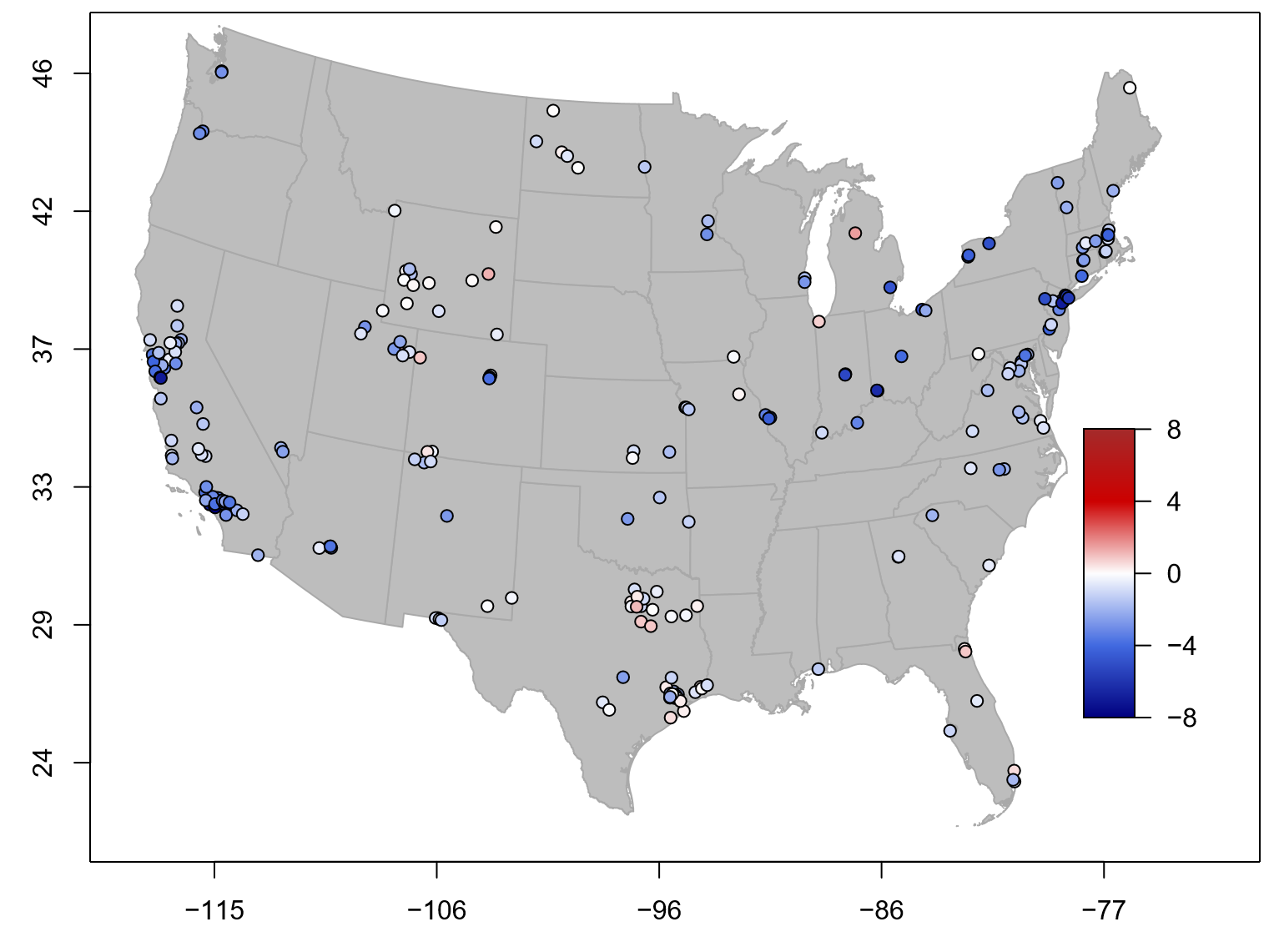
Figure 3: Difference in monthly-average NO2 concentrations (ppb) between April 2020 and the five previous Aprils (2015–2019). Negative values (blue) indicate a decrease in NO2 concentrations in April 2020, vice versa positive values (red) indicate an increase.

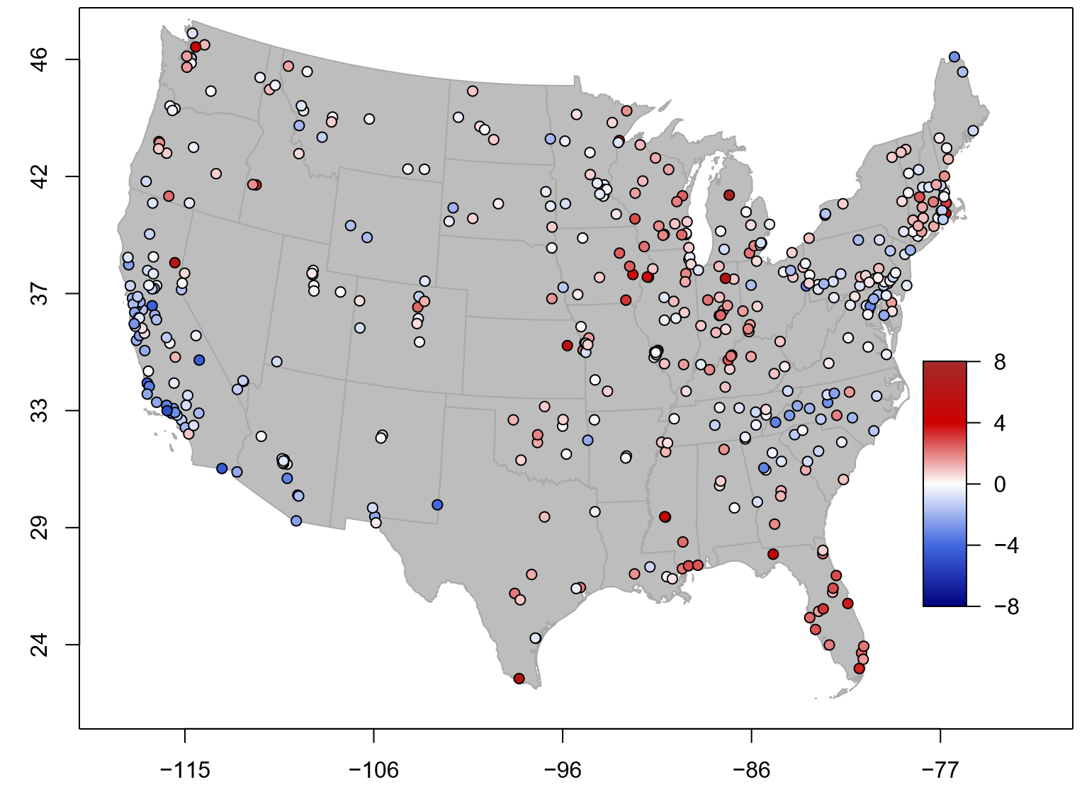
Figure 4: Difference in monthly-average PM_2.5 concentrations ($\mu$g/m³) between April 2020 and the five previous Aprils (2015–2019). Negative values (blue) indicate a decrease in PM_2.5 concentrations in April 2020, vice versa positive values (red) indicate an increase.

An air quality station, whether measuring NO2 or PM_2.5, was used in this study only if it reported both in 2020 (through AirNow) and in the five years prior (through AQS). In addition, only air quality stations that were reporting at least 75% of the time were retained. Note that not all NO2-measuring sites also measure PM_2.5, and vice versa. Of the 426 and 882 sites that measured NO2 and PM_2.5, respectively, in April 2020, only 271 and 819 reported at least 75% of the time, and ultimately only 201 and 480 reported NO2 and PM_2.5 also in April 2015–2019 for at least 75% of the time. These are the sites that we will focus on in this study and that are shown in Figures 3 and 4.

2.2 Satellite data

Satellite observations for NO2 were acquired using the OMI instrument flying onboard the NASA AURA satellite, and were downloaded using the NASA GIOVANNI portal giovanni . Specifically, the Nitrogen Dioxide Product (OMNO2d) was used, which is a Level-3 global gridded product at a 0.25x0.25 spatial resolution provided for all pixels where cloud fraction is less than 30%. The product comes in two variants, the first measuring the concentration in the total column and the second the concentration only in the troposhere. For this work, the latter measurements were used.

The satellite-derived NO2 column totals at the pixels of the ground monitoring sites are well correlated with the NO2 concentrations recorded at the ground monitoring sites in all years, with R-square values varying between 0.76 and 0.80. As an example, we show the correlation between the two in 2016 and 2020 in Figure 1. As such, we can use satellite-derived NO2 column totals to: 1) confirm the results obtained from the ground monitoring sites and 2) analyze pixels where no ground monitoring sites are available.

2.3 Mobility data

Mobility measures aim to capture general patterns of observed movement and most available data products today utilize mobile device activity as a proxy. While policy makers set social distancing guidance, there are various policies enacted and various degrees to which policies are followed throughout the country. We seek to observe actual patterns of movement by using a dataset developed by Descartes Labs descartes that provides an aggregated mobility measure based on anonymized and/or de-identified mobile device locations. Mobility is essentially a statistical representation of the distance a typical member of a given population moves in a day. Descartes Labs calculated the farthest distance apart recorded by smartphone devices utilizing select apps (with location reporting enabled) for at least 10 uses a day, spread out over at least 8 hours in a day, with a day defined as 00:00 to 23:59 local time Warren2020 . The maximum distance for each qualifying device is tied to the origin county in which the anonymized user is first active each day. Aggregated results at the county level are produced as a statistical measure of general travel behavior.

Mobility data are ultimately provided as percent of normal, i.e., the ratio of aggregated mobility during each day of the COVID-19 pandemic over that of the baseline (17 February–7 March 2020). Note that the baseline period is in late winter 2020, whereas the period of focus in this paper is April 2020, in spring. As such, a fraction of the differences in mobility may be due to differences in weather and/or climate rather than to COVID-19 restrictions. We did not attempt to correct for this type of bias. Another caveat, noted by the the producers of the data Warren2020 , is that the raw data used to calculate mobility are available for only a small fraction of the total number of devices (a few percent at most), thus the resulting mobility may or may not truly represent the average behaviour in each county. Nonetheless, the effects of these sampling errors are expected to be small. The mobility data are made freely available by Descartes Labs at the U.S. county level gitdata .

3 Results

3.1 Observed air quality changes

In the rest of this paper, we will compare the monthly-average of the pollutant of interest – NO2 or PM_2.5 – during the month of April 2020 to the average of the five monthly-averages during April of the years 2015 through 2019. There are two reasons for this choice. First, using five years to establish a reference is more meaningful than, say, using just the year 2019, because year-to-year variability can occur regardless of the pandemic. In fact we found that, in general, the year 2019 was relatively clean when compared to the previous five, thus a comparison between April 2020 and April 2019 may under-estimate the true impact of COVID-19. Second, although the monthly-average is not the design value for either NO2 or PM_2.5, it is a value that is representative of the overall air quality during the entire month of April. Alternative metrics, such as the monthly maximum, are more representative of extreme circumstances, like wildfires, that are not necessarily associated to COVID-19.

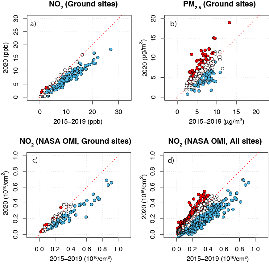
Figure 2: Scatter plots of: (a) NO2 and (b) PM_2.5 observed concentrations at ground monitoring sites, and NO2 column totals from NASA OMI satellite at (c) pixels of the ground monitoring sites and (d) all pixels during April of 2020 (y-axis) versus April of the previous five years 2015–2019 (x-axis). Blue-filled markers represent sites for which the values in April 2020 were lower than in any April of 2015–2019; red-filled markers represent sites for which the values in April 2020 were higher than in any April of 2015–2019.

Starting with NO2, the April 2020 averages were generally below the April 2015–2019 average at the ground monitoring sites, as most sites lay below the 1:1 line in Figure 2b. In addition, 65% of the sites were characterized by NO2 concentrations in 2020 that were lower than those in all of the previous five years (for the month of April). Only a few sites (5 in total, $<2\%$) experienced NO2 concentrations in 2020 that were higher than those in all of the previous five years (for the month of April). The average drop in NO2 concentrations was -2.02 ppb (Tables 1 and 3).

The same pattern is confirmed in the satellite-derived data. Out of the 227 pixels with ground monitoring sites, a total of 127 (56%) exhibited lower NO2in 2020 than in the previous five years and only 5% higher (Figure 2b). Once all 14,706 pixels with valid satellite retrievals all over the country are considered, a similar pattern of lower NO2 column totals in 2020 than in the five previous years emerges from these data too (Figure 2c), but with 28% of the pixels lower in 2020 than in the previous five years and 5% higher (for the month of April, Table 3).

In terms of spatial variability, Figure 3 shows that, although NO2 reductions were recorded all over the country, the highest decreases were observed in California and the Northeast, where the shelter-in-place measures started earlier (March 11 for California, the earliest in the country, and March 22 for New York, third earliest nystats ) and lasted longer (both states still have major restrictions in place as of June 10, 2020 WaPost ). Noticeable exceptions were North Dakota and Wyoming, where either no significant decreases or actual small increases in NO2 concentrations were observed. North Dakota enforced no shelter-in-place measures and in Wyoming only the city of Jackson implemented a stay-at-home order as of April 20, 2020 nystats . However, as discussed in Section 2.3, actual people’s mobility, as opposed to state ordinances, is a better metric to understand the real effect of COVID-19 on air quality because not everybody in all counties followed the state- or county-restrictions all the time.

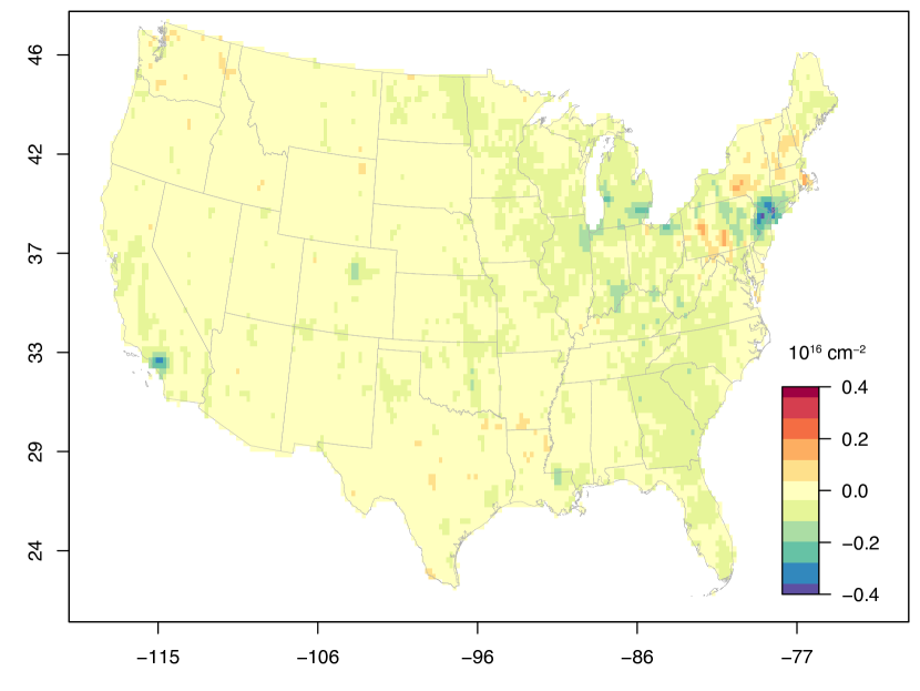
Figure 5: Difference between the NASA OMI NO2 monthly-average column totals ($10^{16}$ molecules/cm²) in 2020 and in 2015–2019 for the month of April. The “hotspot” of reduced NO2 in the Northeast is apparent.

Figure 3 was useful because it included actual NO2 concentrations measured near the ground. However, the spatial coverage was sparse and urban areas were over-sampled compared to rural areas. This weakness is addressed via the NASA OMI satellite data, which are shown in Figure 5 as the difference between the monthly average of NO2 column total in 2020 and that in 2015–2019 for the month of April. The regions with low coverage of ground concentration of NO2 and mobility in the Midwest are generally characterized by near-normal NO2 column totals. The Northeast hotspot of low mobility is also a hotspot of low NO2, consistent with Bauwensetal2020 , although it is surrounded by patches of above-normal values that were not detectable from the ground monitoring stations. The Los Angeles area is another hotspot of NO2 decreases, as for low mobility. For PM_2.5, the ground monitoring stations depict a completely different response to COVID-19. Whereas most NO2 sites were laying below the 1:1 line (Figure 2a), the majority of PM_2.5 sites laid above it (Figure 2b), indicating an overall increase in monthly-average PM_2.5 in the country in April 20202 with respect to the previous five years. Only 18% of the sites reported concentrations of PM_2.5 that were lower in 2020 than in the previous five years (in the month of April), while 24% of the stations reported the highest levels in 2020 compared to the previous five years (for the month of April). The average increase in PM_2.5 concentrations was small, +0.05 $\mu$g/m³ (Tables 2 and 3).

In summary, we report a large decrease (-2.02 ppb, or 27%) in monthly-average NO2 concentrations across the U.S. ground monitoring stations, confirmed by the satellite-derived NO2 column total decrease of 7.1 $\times 10^{14}$ molecules/cm² (or 24%) at the pixels of the ground monitoring stations during April of 2020 when compared to April of the previous five years. When all the pixels with valid data were included, a drop of 2.4$\times 10^{14}$ molecules/cm² (or 13%) during April of 2020 was observed when compared to April of the previous five years (Table 3). The monthly-average of PM_2.5, however, increased slightly on average (+0.05 $\mu$g/m³ when compared to the previous five-year average) during the same period (Table 3). In the next Section 3.3, we try to explain the reasons for these differences.

3.2 Observed mobility changes

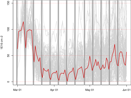
a) b)

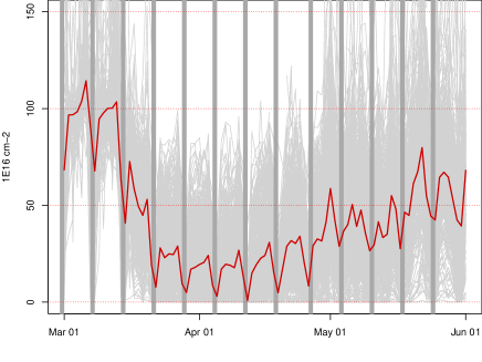
Figure 6: Mobility, expressed as percent of normal, at the locations of the ground stations monitoring (a) NO2 and (b) PM_2.5 during March–May 2020. The average of all the stations is shown in red.

Time series of mobility data at the counties with NO2 ground monitoring sites are shown in Figure 6a and at the counties with PM_2.5 ground monitoring sites in Figure 6b. Only a few counties had both types of monitoring sites, thus the counties included in the two figures are generally different. Yet, the patterns are very similar. First of all, mobility on average dramatically dropped starting in the second half of March, reaching values around 20% by April, and then started to recover in May, as some states reopened for business or relaxed the shelter-in-place measures WaPost . Second, a distinct minimum in mobility during the month of April is clearly visible, which confirms that this month was the most relevant for air quality impacts from COVID-19. There is some variability around this general behaviour, but nonetheless only a few counties barely reached normal mobility in April. Lastly, the typical traffic reduction during the weekends is confirmed in the mobility data, regardless of the pandemic. This adds confidence to the use of mobility data as proxies for people’s actual behaviours.

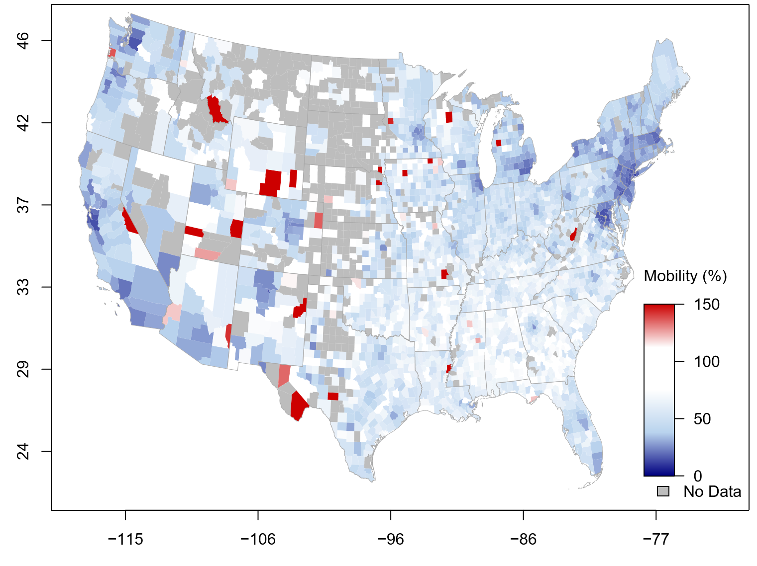
a) b)

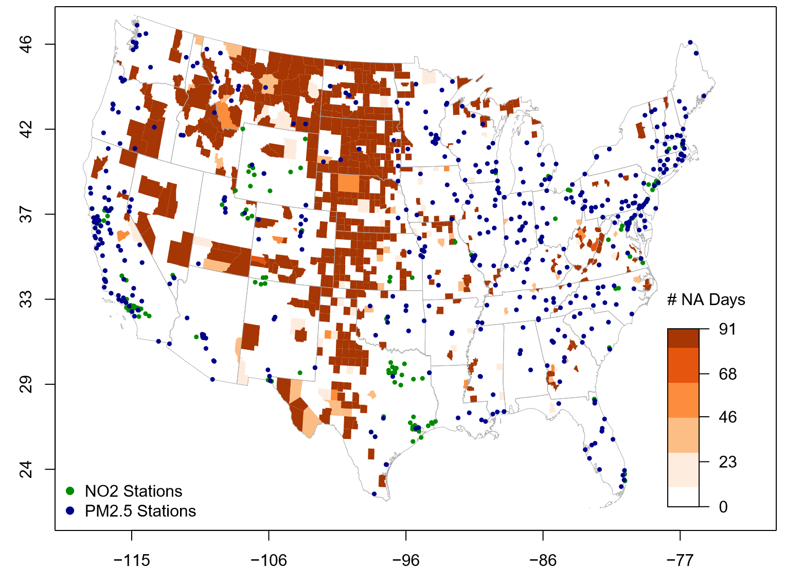
Figure 7: Spatial distribution of (a) mobility, expressed as percent of normal, in April 2020 and (b) mobility data availability, expressed as number of missing days, during March–May 2020.

In terms of spatial variability, changes in mobility during COVID-19 in the U.S. were not uniform, although in general mobility was reduced in most states (Figure 7a). Note the high count of non-valid data in many counties in the Midwest (Figure 7b), possibly due to low population density. However, the ground monitoring stations of both NO2 and PM_2.5 are generally located in counties with high data availability. In general, the strongest decreases in mobility are found around large urban areas throughout the country, e.g., the Northeast corridor from Washington D.C. to Boston; the San Francisco and Los Angeles areas in California; Seattle in the Northwest; and Chicago. A few isolated counties experienced increases in mobility (in red in Figure 7a). Wyoming stands out as one of the few states with no significant decreases in mobility, consistent with the lack of shelter-in-place measures nystats .

3.3 Relationships between air quality and mobility changes

To better interpret the relationship between mobility and the air pollutant of interest, either NO2 or PM_2.5, the mobility data were divided into bins, based on the monthly-average (in April 2020) of the mobility in the county where each ground monitoring site was located. For most cases, there was only one ground monitoring site per county. But in some cases, such as Los Angeles county in California for NO2 or Maricopa county in Arizona for PM_2.5, multiple monitoring sites were located in the same county and therefore they were all paired to the same mobility value. The change in monthly-average concentration of the pollutant between April 2020 and the five previous Aprils was then calculated for each mobility bin.

Starting with NO2, there is a clear relationship with mobility (Figure 8a). Large and negative changes in NO2 concentrations, of the order of -4 ppb, were found at locations where mobility was basically halted, i.e., where it was less than 1% of normal in April 2020, as in full lock down. As mobility increased, the NO2 benefits decreased, although not linearly. For example, decreases by 2–3 ppb in NO2 concentrations occurred where mobility was restricted but not to a full lock down (i.e., between 1% and 20% of normal). Past 20%, the changes in NO2 concentrations were still negative and significant, but not large, less than 1 ppb on average. This suggests that NO2 responds modestly to changes in mobility that are not large, but then, if mobility is reduced dramatically (i.e., by at least 80%, thus it is down to 20% of normal), large decreases in NO2 can occur.

With respect to PM_2.5, there is no obvious relationship between the reductions in mobility and the observed concentrations (Figure 8b). Only for the most extreme mobility reductions, i.e., the bin with $<$1% mobility, which indicates that the entire population was sheltering at home for the entire month of April, PM_2.5 concentrations decreased by about 1 $\mu$g/m³. After the first bin, as mobility increased, both increasing and decreasing concentrations of PM_2.5 were found, with large standard deviations and no discernible pattern. We conclude that the changes in PM_2.5 were not directly caused by changes in people’s mobility.

How can we reconcile the clear relationship of NO2 with mobility with the lack thereof for PM_2.5? The hypothesis we put forward is that the shelter-in-place measures affected mostly people’s driving patterns, thus passenger vehicle – mostly fueled by gasoline – emissions were reduced and so were the resulting concentrations of NO2. Commercial vehicles (generally diesel) and electricity demand for all purposes (often provided by coal-burning power plants), however, remained relatively unchanged, thus PM_2.5 concentrations did not drop significantly and did not correlate with mobility. To test this hypothesis, in a subsequent study we will use a photochemical model, coupled with a numerical weather prediction model, which we will run with and without emissions from diesel vehicles, while keeping everything else the same. The difference between the concentrations of the pollutants in the two cases will be attributable to diesel traffic alone. Similarly, we will be able to reduce emissions from other sectors, to reflect the effect of COVID-19 on other aspects of life, such as air traffic or business closures.

4 Conclusions and future work

This study analyzed the effects of COVID-19 on air quality, more specifically NO2 and fine particulate PM_2.5 concentrations, in the U.S. Although different states introduced different levels of shelter-in-place and social distancing measures at different times, by the beginning of April 2020 all states but a few had adopted some restrictions. As such, the analysis focused on the month of April 2020, which was compared to April of the previous five years, 2015–2019.

Two types of measurements were used, NO2 and PM_2.5 concentrations from the ground monitoring stations – maintained by the states – and satellite-derived NO2 column totals in the troposphere. Although the two measurements are not identical, they are strongly correlated with one another because the near-ground concentrations of NO2 are the dominant contributors to the tropospheric column total.

To quantify social distancing, we used the mobility index calculated and distributed by Descartes Labs. Their algorithms account for people’s maximum distance travelled in a day by tracing the user’s location multiple times a day while using selected apps. Mobility is represented as a percent value, such that 100% means normal conditions, i.e., those during the period of 17 February – 7 March 2020.

We found that NO2 levels decreased significantly in April 2020 when compared to April of the five previous years, by up to 8 ppb in the monthly average at some locations. On average over all U.S. monitoring sites, the decrease in NO2 levels was between 24% (from satellite) and 27% (from ground stations). The decreases in NO2 were largest where mobility was reduced the most, with a direct, although not linear, relationship between the two. In terms of spatial variability, hotspots of reduced NO2 concentrations in the Northeast and California coincided perfectly with hotspots of reduced mobility. Vice versa, states where social distancing measures were minimal experienced the smallest reduction in NO2, e.g., Wyoming and North Dakota.

By contrast, the concentrations of PM_2.5 did not decrease significantly during the same period and even reached unprecedented high values at about a fifth of the sites. In addition, changes in PM_2.5 concentrations were not correlated with changes in people’s mobility, neither spatially nor as aggregated statistics.

We propose that the different response to reduced people’s mobility between NO2 and PM_2.5 could be explained by the fact that commercial vehicles (including delivery trucks, buses, trains), generally diesel fueled, remained more or less in circulation, while passenger vehicles, gasoline fueled, dropped dramatically due to COVID-19. PM_2.5 emissions are much larger from diesel than from gasoline vehicles. In addition, other sources of PM_2.5 emissions, like power plants, did not decrease. We plan to verify this hypothesis in a subsequent study using a photochemical model coupled with a numerical weather prediction model, as described in Section 3.3.

As far as we know, this is the first study to use ground monitoring stations to assess the effects of COVID-19 on air quality in the U.S. Satellite-derived NO2 column totals have been used in a few previous studies, but none looked at the correlation between the two types of NO2 measurements. Another innovation of this study is the use of mobility data, which are an excellent proxy for actual people’s behaviour, as opposed to the state or county regulations, which may or may not be fully followed by people.

This analysis has also numerous limitations. First of all, we paired mobility data and pollutant concentrations at the county level, thus we implicitly assumed that the measured concentration and county-average mobility were representative of the entire county. For large counties, especially those with also low population density, this assumption may not hold. The second implicit assumption of our pairing is that local mobility affects local pollution only and, vice versa, that local pollution is affected by local mobility only. In other words, we are neglecting the effects of transport and chemical reactions, which could cause either an increase or a decrease of pollution regardless of the local mobility change in the county of interest. For example, consider the case that the prevailing wind is such that a county is located downwind of an airport. If the airport was shutdown during the pandemic, that county would see a reduction of NO2 and PM_2.5 concentrations even if no social distancing measures were in place. Another limitation is that we looked at people’s mobility as the only factor explaining NO2 concentration changes, whereas NO2 emissions changed also in response to business and school closures, air traffic reductions, among many others sources. Lastly, we focused on two pollutants only, NO2 and PM_2.5, because of time constraints; future work will include other regulated compounds, such as ozone and carbon monoxide.

Conflict of interest

On behalf of all authors, the corresponding author states that there is no conflict of interest.

Table 1: Monthly-average of NO2 concentrations (ppb) by state in the month of April of the years 2015–2020.

State	N. Sites	2015	2016	2017	2018	2019	2020
Arizona	4	12.49	11.68	13.58	12.82	10.33	9.06
California	56	9.73	9.23	8.79	8.85	8.13	5.92
Colorado	7	11.37	9.87	9.39	9.94	9.5	8.25
Connecticut	3	11.71	11.13	11.72	10.34	8.43	6.54
District Of Columbia	1	9.19	8.74	7.43	8.25	8.46	7.26
Florida	7	5.65	4.23	4.73	5.55	5.34	4.77
Georgia	2	11.39	12.15	10.83	11.62	10.8	10.83
Hawaii	1	3.04	2.99	4.59	3.21	3.72	2.85
Indiana	4	11.49	9.43	8.32	9.89	8.2	7.2
Iowa	1	1.42	2.33	1.66	2.08	1.9	1.69
Kansas	4	6.10	4.86	4.4	5.98	5.16	4.47
Kentucky	1	13.94	14.95	13.08	13.18	17.43	11.25
Maine	2	4.30	3.67	3.99	4.03	3.39	2.83
Maryland	5	10.43	10	8.57	8.84	8.11	6.74
Massachusetts	8	9.47	9.08	7.15	8.45	6.47	5.15
Michigan	2	9.37	8.28	8.37	8.59	7.39	6.79
Minnesota	2	7.51	5.95	7.25	9.88	6.53	5.08
Mississippi	1	3.91	4.25	4.28	3.85	3.79	2.68
Missouri	6	10.81	9.17	8.82	8.62	8.64	6.92
Montana	1	0.54	0.61	0.9	0.68	0.46	0.36
Nevada	2	8.48	7.93	9.77	10.09	8.53	6.76
New Jersey	8	13.80	13.39	12.33	12.48	12.38	8.03
New Mexico	8	4.68	4.56	4.48	4.74	5.22	3.58
New York	5	13.64	12.56	12.05	12.42	11.3	7.55
North Carolina	3	6.04	6.29	6.05	6.11	6.58	4.4
North Dakota	6	2.91	1.98	2.44	2.59	2.16	1.95
Ohio	5	14.60	12.13	10.84	11.17	11.28	8.25
Oklahoma	3	8.89	8.43	7.02	7.38	7.38	6.02
Oregon	2	12.39	11.59	10.69	9.42	9.98	7.77
Pennsylvania	1	12.87	12.89	11.74	10.81	8.7	10.39
Rhode Island	2	14.03	13.5	10.23	13.37	10.15	8.47
South Carolina	2	5.59	6.03	6.73	6.62	5.84	4.92
Texas	40	5.80	6.23	5.23	6.41	5.95	5.26
Utah	7	3.42	2.95	4.5	4.15	2.92	2.32
Vermont	2	7.32	6.12	6.23	6.16	5.74	4
Virginia	9	5.77	5.05	4.92	5.25	5.42	4.04
Washington	2	16.80	18.17	14.25	13.32	11.36	9.52
Wisconsin	2	12.50	11.11	9.61	11.36	9.75	8.63
Wyoming	13	1.69	1.62	1.61	1.55	1.31	1.33

Table 2: Monthly-average of PM_2.5 concentrations ($\mu$g/m³) by state in the month of April of the years 2015–2020.

State	N. Sites	2015	2016	2017	2018	2019	2020
Alabama	4	7.94	7.56	8.82	7.26	7.64	8.59
Alaska	4	3.45	3.57	4.36	3.43	4.45	3.83
Arizona	13	5.67	5.82	6.9	8.13	5.03	4.75
Arkansas	4	7.01	7.12	8.12	6.98	7.51	7.54
California	61	7.06	6.65	6.35	7.93	6.31	5.26
Colorado	8	5.31	3.65	4.63	5.87	5.26	5.21
Connecticut	8	4.8	5.54	3.81	5.61	5.32	5.75
Delaware	3	5.73	5.65	6.21	6.48	5.91	7.09
District Of Columbia	1	6.21	6.68	7.11	8	6.33	4.67
Florida	16	7.01	7	7.41	7.68	6.39	9.52
Georgia	10	7.87	8.31	8.52	8.25	8.83	8.44
Hawaii	7	5.96	4.72	6.68	4.26	3.2	3.32
Idaho	5	4.47	5.51	4.21	4.43	3.55	5.72
Illinois	14	8.23	7.67	7.06	8.03	7.43	8.11
Indiana	15	7.5	8.21	6.17	6.64	6.21	8.47
Iowa	9	7.78	6.97	6.18	7.09	5.65	8.71
Kansas	3	6.34	6.21	6.85	8.31	8.77	11.47
Kentucky	12	6.97	7.03	6.27	6.48	6.77	8.04
Louisiana	4	7.81	7.06	8.43	7.52	6.84	7.74
Maine	6	5.16	5.64	4.93	4.46	3.63	4.05
Maryland	10	6.93	6.75	5.74	6.46	4.33	4.81
Massachusetts	9	4.67	5.08	3.02	5.6	4.68	5.71
Michigan	11	6.7	6.7	5.52	6.48	6.33	7.1
Minnesota	18	5.09	5.66	5.06	6.22	4.88	5.73
Mississippi	7	7.98	7.49	8.32	8.27	6.97	10.15
Missouri	13	7.65	6.3	6.46	7.33	7.33	6.6
Montana	11	5.02	4.57	4.07	4.81	3.7	4.21
Nebraska	2	8.02	6.65	9.82	9.77	6.1	8.17
Nevada	6	6.16	4.81	4.57	5.25	3.23	4.11
New Hampshire	5	4.3	4.2	3.18	4.11	3.34	4.01
New Jersey	3	5.69	7.27	7.32	7.17	6.09	5.84
New Mexico	5	7.34	5.05	7.02	7.93	5.58	4.87
New York	7	5.32	4.99	4.38	4.93	4.92	4.5
North Carolina	13	6.78	7.25	7.16	6.53	6.4	5.41
North Dakota	6	4.65	3.24	4.33	5.26	3.58	4.2
Ohio	12	7.49	7.86	5.55	6.82	6.68	6.99
Oklahoma	9	7.32	7.31	7.52	8.78	7.71	8.19
Oregon	12	5.3	4.94	4.28	5.14	4.24	5.17
Pennsylvania	24	7.41	7.01	7.64	6.99	6.52	6.97
Rhode Island	5	4.84	5.2	4.56	6.01	3.3	4.08
South Carolina	6	7.33	6.95	7.95	6.64	6.6	6.62
South Dakota	8	6.65	4.93	5.35	5.54	3.68	5.01
Tennessee	11	6.41	6.68	6.8	6.45	6.5	6.23
Texas	11	10.04	8.84	9.13	8.79	8.76	10.27
Utah	7	5.6	3.3	3.47	4.59	3.03	3.79
Vermont	4	4.32	4.24	3.27	4.69	4.48	4.73
Virginia	6	5.74	5.76	6.33	5.31	5.75	5.66
Washington	11	5.57	6.5	3.53	4.01	4.17	5.11
Wisconsin	18	5.45	7.47	4.58	5.46	6.68	7.49
Wyoming	3	4.04	2.75	2.73	3.3	2.57	1.73

Table 3: Average air quality measurements in April of the years 2015–2020 from NASA OMI and ground monitoring stations.

	2015	2016	2017	2018	2019	2020
NASA OMI
NO2 at all pixels (1016molecules/cm2)	0.16	0.15	0.14	0.13	0.14	0.12
NO2 at ground sites (1016molecules/cm2)	0.32	0.31	0.28	0.29	0.29	0.23
Ground monitoring stations
NO2 (ppb)	8.16	7.69	7.22	7.62	7.0	5.52
PM_2.5 ($\mu$g/m3)	6.52	6.36	6.02	6.60	5.82	6.31

a) b)

Figure 1: Scatter plots of monthly-average NO2 concentrations (ppb) from the ground monitoring sites versus monthly-average NO2 column totals ($10^{16}$ molecules/cm²) retrieved from the NASA OMI satellite at the pixels of the ground monitoring sites during (a) April 2016 and (b) April 2020.

a) b)

Figure 8: Changes in monthly-average concentrations of (a) NO2 and (b) PM_2.5 near ground monitoring sites during April of 2020 versus April of the previous five years as a function of mobility index bins in April 2020.

References

- (1) Bao, R., Zhang, A.: Does lockdown reduce air pollution? Evidence from 44 cities in northern China. Science of the Total Environment p. 139052 (2020). DOI 10.1016/j.scitotenv.2020.139052
- (2) Bauwens, M., Compernolle, S., Stavrakou, T., Müller, J.F., van Gent, J., Eskes, H., Levelt, P.F., van der A, R., Veefkind, J.P., Vlietinck, J., Yu, H., Zehner, C.: Impact of coronavirus outbreak on NO2 pollution assessed using TROPOMI and OMI observations. Geophysical Research Letters 47(11), e2020GL087978 (2020). DOI 10.1029/2020GL087978. https://agupubs.onlinelibrary.wiley.com/doi/abs/10.1029/2020GL087978
- (3) Beydoun, M., Eslami, E., Jennings, M.: HARC research analyzes effects of COVID-19 on air quality. Tech. rep., Houston Advanced Research Center (HARC) (April 29, 2020). https://www.newswise.com/coronavirus/harc-research-analyzes-effects-of-covid-19-on-air-quality/?article_id=730812
- (4) British Broadcasting Corporation (BBC): Earlier coronavirus lockdown could have saved 36,000 lives (May 2020). https://www.bbc.com/news/world-us-canada-52757150, Accessed 06/09/2020
- (5) Burke, M.: COVID-19 reduces economic activity, which reduces pollution, which saves lives (March 8, 2020). http://www.g-feed.com/2020/03/covid-19-reduces-economic-activity.html, Accessed 06/09/2020
- (6) Center for Disease Control and Prevention (CDC): Coronavirus Disease 2019 (COVID-19): Cases in the US (June 8, 2020). https://www.cdc.gov/coronavirus/2019-ncov/cases-updates/cases-in-us.html, Accessed 06/09/2020
- (7) Chan, J.F.W., Yuan, S., Kok, K.H., To, K.K.W., Chu, H., Yang, J., Xing, F., Liu, J., Yip, C.C.Y., Poon, R.W.S., et al.: A familial cluster of pneumonia associated with the 2019 novel coronavirus indicating person-to-person transmission: a study of a family cluster. The Lancet 395(10223), 514–523 (2020)
- (8) Chen, K., Wang, M., Huang, C., Kinney, P.L., Anastas, P.T.: Air pollution reduction and mortality benefit during the COVID-19 outbreak in China. The Lancet Planetary Health (2020). DOI 10.1016/S2542-5196(20)30107-8
- (9) Dantas, G., Siciliano, B., França, B.B., da Silva, C.M., Arbilla, G.: The impact of COVID-19 partial lockdown on the air quality of the city of Rio de Janeiro, Brazil. Science of the Total Environment 729, 139085 (2020)
- (10) Descartes Labs: Mobility changes in response to COVID-19. https://github.com/descarteslabs/DL-COVID-19, Accessed 06/01/2020
- (11) Descartes Labs: U.S. mobility. https://www.descarteslabs.com/mobility/, Accessed 06/10/2020
- (12) Dutheil, F., Baker, J.S., Navel, V.: COVID-19 as a factor influencing air pollution? Environmental Pollution 263, 114466 (2020)
- (13) European Space Agency (ESA): Coronavirus lockdown leading to drop in pollution across Europe (March 27, 2020). https://www.esa.int/Applications/Observing_the_Earth/Copernicus/Sentinel-5P/Coronavirus_lockdown_leading_to_drop_in_pollution_across_Europe, Accessed 06/10/2020
- (14) Gao, S., Rao, J., Kang, Y., Liang, Y., Kruse, J.: Mapping county-level mobility pattern changes in the United States in response to COVID-19. SIGSPATIAL Special 12(1), 16–26 (2020)
- (15) Isaifan, R.: The dramatic impact of coronavirus outbreak on air quality: Has it saved as much as it has killed so far? Global Journal of Environmental Science and Management 6(3), 275–288 (2020)
- (16) Johns Hopkins University: COVID-19 dashboard by the Center for Systems Science and Engineering (CSSE) at Johns Hopkins University (JHU) (2020). https://coronavirus.jhu.edu/map.html, accessed 06/16/2020
- (17) Kerimray, A., Baimatova, N., Ibragimova, O.P., Bukenov, B., Kenessov, B., Plotitsyn, P., Karaca, F.: Assessing air quality changes in large cities during COVID-19 lockdowns: The impacts of traffic-free urban conditions in Almaty, Kazakhstan. Science of the Total Environment p. 139179 (2020)
- (18) Le Quéré, C., Jackson, R.B., Jones, M.W., Smith, A.J., Abernethy, S., Andrew, R.M., De-Gol, A.J., Willis, D.R., Shan, Y., Canadell, J.G., et al.: Temporary reduction in daily global \ceCO2 emissions during the COVID-19 forced confinement. Nature Climate Change pp. 1–7 (2020)
- (19) Lin, J.T., McElroy, M.B.: Detection from space of a reduction in anthropogenic emissions of nitrogen oxides during the chinese economic downturn. Atmospheric Chemistry and Physics (2011)
- (20) Mahato, S., Pal, S., Ghosh, K.G.: Effect of lockdown amid COVID-19 pandemic on air quality of the megacity Delhi, India. Science of the Total Environment p. 139086 (2020)
- (21) Mervosh, S., Lu, D., Swales, V.: See which states and cities have told residents to stay at home (April 20, 2020). https://www.nytimes.com/interactive/2020/us/coronavirus-stay-at-home-order.html, Accessed 06/13/2020
- (22) Mullen, B.: COVID-19 clinical guidance for the cardiovascular care team. Tech. rep., American College of Cardiology (ACC) (March 6, 2020). https://www.acc.org/~/media/665AFA1E710B4B3293138D14BE8D1213.pdf
- (23) Nakada, L.Y.K., Urban, R.C.: COVID-19 pandemic: Impacts on the air quality during the partial lockdown in São Paulo state, Brazil. Science of The Total Environment p. 139087 (2020)
- (24) National Aeronautics and Space Administration (NASA): NASA probes environment, COVID-19 impacts, possible links (April 29, 2020). https://www.nasa.gov/feature/nasa-probes-environment-covid-19-impacts-possible-links, Accessed 06/10/2020
- (25) Nemati, M., Ebrahimi, B., Nemati, F.: Assessment of Iranian nurses’ knowledge and anxiety toward COVID-19 during the current outbreak in Iran. Archives of Clinical Infectious Diseases 15(COVID-19) (2020)
- (26) New York State Department of Environmental Conservation: Air monitoring website. http://www.nyaqinow.net/, Accessed 05/07/2020
- (27) Pishue, B.: COVID-19’s impact on freight: An analysis of long-haul freight movement during a pandemic. Tech. rep., INRIX (April 28, 2020)
- (28) Plumer, B., Popovich, N.: Traffic and pollution plummet as U.S. cities shut down for coronavirus (March 2020). https://www.nytimes.com/interactive/2020/03/22/climate/coronavirus-usa-traffic.html?auth=link-dismiss-google1tap, Accessed 06/09/2020
- (29) Sharma, S., Zhang, M., Gao, J., Zhang, H., Kota, S.H., et al.: Effect of restricted emissions during COVID-19 on air quality in India. Science of the Total Environment 728, 138878 (2020)
- (30) Shi, X., Brasseur, G.P.: The response in air quality to the reduction of Chinese economic activities during the COVID-19 outbreak. Geophysical Research Letters 47(11), e2020GL088070 (2020). DOI 10.1029/2020GL088070. https://agupubs.onlinelibrary.wiley.com/doi/abs/10.1029/2020GL088070
- (31) Slotnick, D.: Coronavirus demolished air travel around the globe. These 14 charts show how empty the skies are right now (April 22, 2020). https://www.businessinsider.com/air-traffic-during-coronavirus-pandemic-changes-effects-around-the-world-2020-4, Accessed 06/10/2020
- (32) Texas Commission on Environmental Quality (TCEQ): Monthly summary report by site. https://www.tceq.texas.gov/cgi-bin/compliance/monops/select_month.pl, Accessed 06/12/2020
- (33) The Washington Post: Where states are reopening after the U.S. shutdown (June 2020). https://www.washingtonpost.com/graphics/2020/national/states-reopening-coronavirus-map/, Accessed 06/09/2020
- (34) Tobías, A., Carnerero, C., Reche, C., Massagué, J., Via, M., Minguillón, M.C., Alastuey, A., Querol, X.: Changes in air quality during the lockdown in Barcelona (Spain) one month into the SARS-CoV-2 epidemic. Science of the Total Environment p. 138540 (2020)
- (35) U.S. Environmental Protection Agency (EPA): Nitrogen dioxide (\ceNO2) pollution. https://www.epa.gov/no2-pollution/basic-information-about-no2#What%20is%20NO2, Accessed 06/10/2020
- (36) U.S. Environmental Protection Agency (EPA): Particulate Matter (\cePM) pollution. https://www.epa.gov/pm-pollution/particulate-matter-pm-basics#PM, Accessed 06/10/2020
- (37) U.S. Environmental Protection Agency (EPA): Profile of version 1 of the 2014 national emissions inventory. Tech. rep., Office of Air Quality Planning and Standards (2017). https://www.epa.gov/sites/production/files/2017-04/documents/2014neiv1_profile_final_april182017.pdf, Accessed 06/17/2020
- (38) U.S. Environmental Protection Agency (EPA) Air Quality System: Pre-generated data files. https://aqs.epa.gov/aqsweb/airdata/download_files.html, Accessed 5/20/2020
- (39) U.S. Environmental Protection Agency (EPA) AirNow: AirNow API. https://docs.airnowapi.org/, Accessed 5/27/2020
- (40) U.S. National Aeronautics and Space Administration (NASA), Earth Science Data Systems (ESDS): Giovanni, The bridge between data and science. https://giovanni.gsfc.nasa.gov/giovanni/, Accessed 05/30/2020
- (41) Warren, M.S., Skillman, S.W.: Mobility changes in response to COVID-19. Tech. rep., Descartes Labs (2020). DOI arxiv.org/abs/2003.14228. Available at https://www.descarteslabs.com/wp-content/uploads/2020/03/mobility-v097.pdf
- (42) Worden, H., Martínez-Alonso, S., Park, M., Pan, L.: COVID-19 impact on Asian emissions: Insight from space observations (March 2020). https://www2.acom.ucar.edu/news/covid-19-impact-asian-emissions-insight-space-observations, Accessed 06/09/2020
- (43) World Health Organization (Regional Office for Europe): WHO announces COVID-19 outbreak a pandemic (March 2020). http://www.euro.who.int/en/health-topics/health-emergencies/coronavirus-covid-19/news/news/2020/3/who-announces-covid-19-outbreak-a-pandemic, Accessed 06/09/2020
- (44) World Health Organization (WHO): Coronavirus disease 2019 (COVID-19) situation report – 94 (Apr 2020). https://www.who.int/docs/default-source/coronaviruse/situation-reports/20200423-sitrep-94-covid-19.pdf?sfvrsn=b8304bf0_2, Accessed 06/09/2020
- (45) World Heath Organization (WHO): Air pollution. https://www.who.int/health-topics/air-pollution#tab=tab_1, Accessed 06/10/2020
- (46) Worldometers.info: COVID-19 coronavirus pandemic (June 9, 2020). https://www.worldometers.info/coronavirus/, Accessed 06/09/2020
- (47) Wu, X., Nethery, R.C., Sabath, B.M., Braun, D., Dominici, F.: Exposure to air pollution and COVID-19 mortality in the United States. medRxiv (2020). DOI 10.1101/2020.04.05.20054502
- (48) Yongjian, Z., Jingu, X., Fengming, H., Liqing, C.: Association between short-term exposure to air pollution and COVID-19 infection: Evidence from China. Science of the total environment p. 138704 (2020)
- (49) Zambrano-Monserrate, M.A., Ruano, M.A., Sanchez-Alcalde, L.: Indirect effects of COVID-19 on the environment. Science of The Total Environment p. 138813 (2020)
- (50) Zhang, R., Zhang, Y., Lin, H., Feng, X., Fu, T.M., Wang, Y.: \ceNOx emission reduction and recovery during COVID-19 in east China. Atmosphere 11(4), 433 (2020)