Cutting Polygons into Small Pieces with Chords:
Laser-Based Localization

Abstract

Motivated by indoor localization by tripwire lasers, we study the problem of cutting a polygon into small-size pieces, using the chords of the polygon. Several versions are considered, depending on the definition of the “size” of a piece. In particular, we consider the area, the diameter, and the radius of the largest inscribed circle as a measure of the size of a piece. We also consider different objectives, either minimizing the maximum size of a piece for a given number of chords, or minimizing the number of chords that achieve a given size threshold for the pieces. We give hardness results for polygons with holes and approximation algorithms for multiple variants of the problem.

1 Introduction

Indoor localization is a challenging and important problem. While GPS technology is very effective outdoors, it generally performs poorly inside buildings, since GPS depends on line-of-sight to satellites. Thus, other techniques are being considered for indoor settings. One of the options being investigated for localization and tracking is to use one-dimensional tripwire sensors [18] such as laser beams, video cameras with a narrow field of view [35], and pyroelectric or infrared sensors [14, 16]. In these approaches, multiple sensors emitting directional signal beams are deployed in an environment, with the beams inducing an arrangement that cuts the domain into cells, allowing one to track the movement of a mobile target from one cell to another when it crosses the signal beam. Since the accuracy of the localization depends on the sizes of the cells, it is desirable to cut the polygon into small pieces. With such beam deployment, one can also ensure that no “large” object can be “hidden” in the domain, since any such object will necessarily intersect one of the beams.

In the literature there have been studies of target localization and tracking using such “tripwire” sensors. Zheng, Brady, and Agarwal [36] consider general models of “boundary sensors” that are triggered when an object crosses them. They assume that the position of the sensors is already given and consider the signal processing problem of determining the location and trace of a target by the spatial and temporal sequence of the laser beams crossed by the target. In this paper, we focus on the problem of optimizing the placement of signal beam sensors to minimize the ambiguity of target location within each cell.

Problem Formulation and Notation.

We study various versions of the laser cutting problem. The input polygon, denoted by $P$, is a closed polygonal domain (i.e., a connected compact set in $\mathbb{R}^{2}$ with piecewise linear boundary) having a total of $n$ vertices, $r$ of which are reflex (having internal angle greater than $\pi$). The terms “cut” and “laser” will be used interchangeably to denote a chord of $P$, i.e., a maximal line segment in $P$ whose relative interior lies in the interior of $P$. The measure (or size) of a cell in the arrangement will be (a) the cell’s area, (b) its diameter (defined as the maximum Euclidean distance between two points of the cell), or (c) the radius of the largest inscribed disk within the cell.

For each measure, we consider two formulations of the optimization problem:

• MinMeasure: Given a positive integer $k$, determine how to place $k$ laser beams in $P$ to minimize the maximum measure, $\delta$, of a cell in the arrangement of the lasers.

• Min-LaserMeasure: Given $\delta>0$, determine the smallest number of laser beams to cut $P$ into cells each of measure at most $\delta$.

In Min-LaserMeasure, no generality is lost by taking the cell size bound, $\delta$, to be 1. We assume that the optimal solution is greater than a constant $c$; otherwise, the problem can be solved optimally in $O(n^{\textrm{poly}(c)})$ time (in the real RAM model of computation, standard for geometric algorithms) by reducing it to a mathematical program whose variables are the locations of the lasers endpoints on the boundary of $P$ (the space of the variables would be split into regions of fixed combinatorial types for all the lasers, and in each region, the measures for the cells of the partition of $P$ will be explicitly written and optimized—since each cell has $\textrm{poly}(c)=O(1)$ complexity, the optimization problem will be of constant size). It may be interesting to investigate also the opposite scenario and obtain efficient algorithms for minimizing the measures using a small given number of lasers. Further variants of the problem may be defined. One possible requirement is to use only axis-aligned lasers—in fact, with this restriction (of primarily theoretical interest) we obtain better approximations than for the more general case of unrestricted-orientation lasers.

Results.

We give hardness results and approximation algorithms for several variants of the problems, using a variety of techniques. Specifically,

• Section 2 proves hardness of our problems in polygons with holes: we show that it is NP-hard to decide whether one can split the domain into pieces of measure at most $\delta$, using a given number $k$ of lasers (this holds for any of the measures, which implies that both MinMeasure and Min-LaserMeasure are hard for polygons with holes). Our hardness reductions hold using axis-parallel lasers, as well, which implies that the problem is hard with or without the restriction to axis-aligned lasers.

• Section 3.1 gives an $O(\log r)$-approximation for Min-LaserArea in simple polygons. The algorithm “unrefines” the ray shooting subdivision by Hershberger and Suri [19], merging the triangles bottom-up along the decomposition tree; the merging stops whenever the next merge would create a cell of area greater than $\delta$, implying that the boundaries between the merged cells can be charged to disjoint parts of $P$ of area more than $\delta$. The lasers are then put along the cell boundaries of the coarsened subdivision; since the subdivision is obtained by cutting out $O(1)$ children from parents in a tree on the original subdivision (where the children were separated from parents by polygonal chains of $O(1)$ complexity), we can charge these $O(1)$ lasers to the intersection of OPT with an area of more than $\delta$. The remaining large pieces in the coarsened subdivision (e.g., triangles of area more than $\delta$ in the initial triangulation) are cut with a suitable grid of lasers, which is within a constant factor of optimal subdivision for each piece. The $O(\log n)$ approximation factor then follows from the fact that each laser could pass through $O(\log n)$ cells of the original subdivision (the subdivision’s core property). To bring the approximation factor down to $O(\log r)$ we decompose $P$ into convex pieces with a decomposition whose stabbing number is $O(\log r)$ (a result, which may be of independent interest) and use the same scheme as with the Hershberger–Suri decomposition.

• In Section 4.1 we present a bi-criteria approximation to the diameter version for simple polygons: if $k$ lasers can cut $P$ into pieces of diameter at most $\delta$, we find a cutting with at most 2$k$ lasers into $O(\delta)$-diameter pieces. In Section 4.2 we use the bi-criteria algorithm to give a constant-factor approximation to MinDiameter. Both algorithms use only axis-aligned lasers, yielding the same approximation guarantees for the versions with general-direction lasers and with axis-aligned lasers.

• Section 5 gives a constant-factor approximation to Min-LaserDiameter and Min-LaserArea in simple polygons under the restriction that the lasers are axis-aligned. The algorithms are based on “histogram decomposition” with constant stabbing number and solving the problems in each histogram separately.

• In Section 6 we give a bi-criteria approximation to the diameter version in polygons with holes under the restriction that lasers are axis-parallel. The algorithm is similar to the one for simple polygons in that they both use a grid; however, everything else is different: in simple polygons we place lasers along grid lines, while in polygons with holes the grid lines just subdivide the problem (in fact, we consider the vertical and the horizontal strips separately). More importantly, even though we place axis-aligned lasers in both simple and nonsimple polygons, for the former we approximate cutting with arbitrary-direction lasers, while for the latter only cuttings with axis-aligned lasers (approximating cuttings with general-direction lasers in polygons with holes is open). We use the bi-criteria algorithm to give a constant-factor approximation to MinDiameter in polygons with holes—this part is the same as for simple polygons.

• Section 7 gives an $O(\log{\rm OPT})$-approximation for Min-LaserCircle in polygons with holes. The algorithm is based on a reduction to the SetCover problem.

Table 1 summarizes our results. The running times of our algorithms depend on the output complexity, which may depend on the size (area, perimeter, etc.) of $P$. Some of our algorithms can be straightforwardly made to run in strongly-polynomial time, producing a strongly-polynomial-size representation of the output; for others, such conversion—which in general is outside our scope—is not easily seen. Many versions of the problem still remain open. For simple polygons, despite considerable attempts, we have neither hardness results nor polynomial-time algorithms to compute an optimal solution; all of our positive results are approximation algorithms.

	Axis-Parallel Lasers		Unrestricted-Direction Lasers
	Min-LaserMeasure	MinMeasure	Min-LaserMeasure	MinMeasure
Area	$O(1)$ 5	OPEN	$O(\log r)$ 3.1	OPEN
Diameter	$O(1)$ 5	$O(1)$* 4.2, 6	bi-critreria 4.1	$O(1)$ 4.2
In-circle radius	$O(\log\mbox{OPT})$* 7	OPEN	$O(\log\mbox{OPT})$* 7	OPEN

Table 1: Approximations for simple polygons. The results marked with asterisks apply also to polygons with holes (either directly or with a similar/extended algorithm).

Related Previous Work. Previous results on polygon decomposition [24] use models that do not support laser cuts or are restricted to convex bodies. For example, Borsuk’s conjecture [6, 20, 22] seeks to partition a convex body of unit diameter in $\mathbb{R}^{d}$ into the minimum number of pieces of diameter less than one. Conway’s fried potato problem [10, 4] seeks to minimize the maximum in-radius of a piece after a given number of successive cuts by hyperplanes for a convex input polyhedron in $\mathbb{R}^{d}$. Croft et al. [10, Problem C1] raised a variant of the problem in which a convex body is partitioned by an arrangement of hyperplanes (i.e., our problem in $\mathbb{R}^{d}$), but no results have been presented.

Equipartition problems ask to partition convex polygons into convex pieces all having the same area or the same perimeter (or other measures) [2, 5, 23, 25, 30, 32]. In these problems, the partition is not restricted to chords (or hyperplanes). Topological methods are used for existential results in this area, and very few algorithmic results are known [1]. Another related problem is the family of so-called cake cutting problems [31, 15], in which an infinite straight line “knife” is used to cut a convex “cake” into (convex) pieces that represent a “fair” division into portions. In contrast, we are interested in cutting nonconvex polygons into connected pieces.

In [7] several variants of Chazelle’s result from [9] were explored, including cutting the polygon along a chord to get approximately equal areas of the two resulting parts. Yet another related problem is that of “shattering” with arrangements [13], in which one seeks to isolate objects in cells of an arrangement of a small number of lines, but without consideration of the size of the cells (as is important in our problem).

2 Hardness in Polygons with Holes

We show that for all three measures (area, diameter, the radius of the largest inscribed circle) it is NP-hard to decide whether a given polygon $P$ with holes can be divided into pieces of small measure using a given number of lasers, both for unrestricted-orientation and axis-aligned lasers. However, it is currently open whether these problems remain NP-hard for simple polygons.

We prove hardness by reduction from the 3SAT problem. Our polynomial-time reduction is similar to previous reductions for line cover problems, which are geometric variants of set cover [26]. In particular, Megiddo and Tamir [28] proved that the LineCover problem is NP-complete: Given $n$ points in the plane and an integer $k$, decide whether the points can be covered by $k$ lines. Hassin and Megiddo [17] proved hardness for MinimumHittingHorizontalUnitSegments problem: Given $n$ horizontal line segments in the plane, each of unit length, and an integer $k$, decide whether there exists a set of $k$ axis-parallel lines that intersects all $n$ segments. Our reduction is based on the idea of Hassin and Megiddo, but requires some adjustments to generate a subdivision of a polygon.

Theorem 1.

In a polygon with holes, both MinArea and Min-LaserArea are NP-hard (with or without the axis-aligned lasers restriction).

Proof.

We reduce from 3-SAT. Let $\Phi$ be a boolean formula in 3CNF with $m$ clauses $c_{1},\ldots,c_{m}$, and $n$ variables $x_{1},\ldots,x_{n}$. We construct an orthogonal polygon $P$ with holes and an integer $k$ such that $\Phi$ is satisfiable if and only if $P$ can be subdivided into regions of area at most $2$ using $k$ lasers. (The reduction goes through with or without the restriction that all lasers are axis-parallel).

We construct a polygon $P$ from the rectangle $B=[0,7m+2]\times[0,3n+4]$ by carving rectangular “rooms” connected by narrow corridors. The rooms are pairwise disjoint and they each have area of $2$. The corridors are axis-parallel, run between opposite sides of the bounding box $B$, and their width is $1/(100\max\{m,n\})$. See Fig. 1 for an illustration.

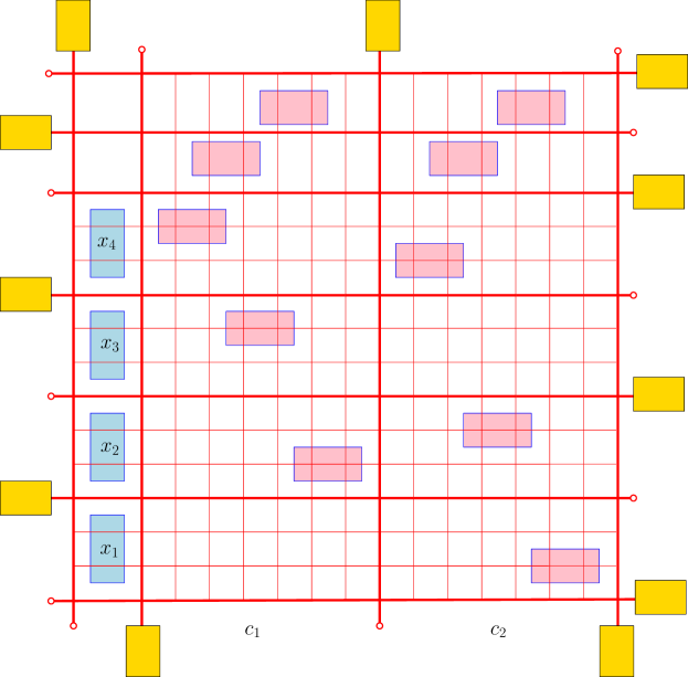
Figure 1: An example for the rooms and corridors for $\Phi=(x_{2}\vee\overline{x}_{3}\vee\overline{x}_{4})\wedge(x_{1}\vee\overline{x}_{2}\vee x_{4})$. The rooms corresponding to variables are in blue. The rooms corresponding to clauses (five rooms per clause) are in pink. The corridors are shown in red, some of which are connected to additional rooms (shown in yellow). The polygon is composed of the union of all the rooms and corridors.

Variable rooms. For each variable $x_{i}$, $i=1,\ldots,n$, create one room: $[\frac{1}{2},\frac{3}{2}]\times[3(i-1)+\frac{1}{2},3i-\frac{1}{2}]$. Note that all rooms are to the left of the line $x=2$.

Clause rooms. For each clause $c_{j}$, $j=1,\ldots,m$, create five rooms. All five rooms have size $2\times 1$ and lie between the lines $x=7(j-1)+2$ and $x=7j+2$. Three out of five rooms are aligned with the variable rooms. Suppose $c_{j}$ contains the variables $x_{i}$, $x_{i^{\prime}}$, and $x_{i^{\prime\prime}}$, where $i<i^{\prime}<i^{\prime\prime}$. If $x_{i}$ is nonnegated, then create the room $[7(j-1)+\frac{1}{2},7(j-1)+\frac{5}{2}]\times[3(i-1)+\frac{1}{2},3i-\frac{3}{2}]$; otherwise create the room $[7(j-1)+\frac{1}{2},7(j-1)+\frac{5}{2}]\times[3(i-1)+\frac{3}{2},3i-\frac{1}{2}]$. We create a room for $x_{i^{\prime}}$ (resp., $x_{i^{\prime\prime}}$) analogously, shifted by a horizontal vector $(0,2)$ (resp;., $(0,4)$). Note that the $x$-projections of these rectangles do not overlap. Two additional rooms lie above the variable rooms: $[7(j-1)+\frac{3}{2},7(j-1)+\frac{7}{2}]\times[2n+\frac{1}{2},2n+\frac{3}{2}]$ and $[7(j-1)+\frac{7}{2},7(j-1)+\frac{11}{2}]\times[2n+\frac{5}{2},2n+\frac{7}{2}]$.

Corridors and separator gadgets. Create narrow corridors along the vertical lines $x=0,2,3,\ldots,7m$ and horizontal lines $y=0,1,2,\ldots,3n$, $y=3n+2$, and $y=3n+4$. Add rectangular rooms of area $2$ at one end of some of the corridors. Specifically, we add rooms to the corridors at $x=0$ and $x=7j+2$ for $j=0,1,\ldots,m$ alternately at the top and bottom endpoints; and similarly for the corridors at $y=3i$ for $i=0,1,\ldots,n$, $y=3n+2$, and $y=3n+4$, alternately at the left and right endpoints. Altogether, $m+n+5$ corridors have rooms at their endpoints.

Finally, we set the parameter $k=3m+2n+5$. This completes the description of an instance corresponding to the Boolean formula $\Phi$.

Equivalence. Let $\tau:x_{i}\rightarrow\{\texttt{true},\texttt{false}\}$ be a satisfying truth assignment for $\Phi$. We show that $P$ can be subdivided by $k$ lasers into regions of area at most $2$. Place lasers at all horizontal and vertical lines that have additional rooms at their endpoints; this requires $m+n+5$ lasers. These lasers subdivide $P$ into subpolygons that each intersect at most one room. For $i=1,\ldots,n$, if $\tau(x_{i})=\texttt{true}$, then place a horizontal laser at $y=3(i-1)+1$ (along the bottom corridor touching room for $x_{i}$), otherwise at $y=3(i-1)+2$ (along the top corridor touching room for $x_{i}$). These lasers split each variable room into two rectangles of area $\frac{1}{2}$ and $\frac{3}{2}$. For $j=1,\ldots,m$, we place two vertical lasers that subdivide the rooms associated with clause $c_{j}$. Since $\tau$ is a satisfying truth assignment, the rooms corresponding to true literals are already split by horizontal lasers. As can easily be checked, the remaining (at most 4) rooms can be split using two vertical lasers. Now $P$ is subdivided into pieces that each intersect at most one room, and contains at most $1.5$ area of each room. Since the corridors are narrow, the area of each piece is less than 2, as required. We have used $n$ horizontal lasers for the variables, and $2m$ vertical lasers for clauses. Overall, we have used $(m+n+5)+n+2m=3m+2n+5$ lasers.
Suppose now that $k=3m+2n+5$ lasers can subdivide $P$ into polygons of area at most 2. We show that $\Phi$ is satisfiable. The area of each room is about 2, so they each intersect at least one laser. Each variable room requires at least one laser; and the $n$ variable rooms jointly require $n$ lasers (as no laser can intersects two variable rooms). Each clause is associated with two rooms above the line $y=3n$; which jointly require two lasers. Overall these rooms require $2m$ lasers.

Note that a laser that intersects a clause rooms above $y=3n$ or a variable room cannot intersect any room at the end of corridors. We are left with at most $k-(n+2m)=m+n+5$ lasers to split these rooms. Since we have precisely $m+n+5$ rooms at the end of the corridors, and no laser can intersect two such rooms, there is a unique laser intersecting each of these rooms. As argued above, for $i=1,\ldots,n$, the room associated with $x_{i}$ intersects only one laser. If this laser intersects the corridor at $y=3(i-1)+1$, then let $\tau(x_{i})=\texttt{true}$, otherwise $\tau(x_{i})=\texttt{false}$. For $j=1,\ldots,m$, there are two lasers that intersect the two rooms associated with $c_{j}$ above $y=3n$. These two lasers cannot intersect all three rooms associated with $c_{j}$ below $y=3n$. Consequently, at least one of these rooms intersects a laser coming from a variable room. Hence each clause contains a true literal, and $\Phi$ is satisfiable. ∎

Theorem 2.

In polygons with holes, both MinCircle and Min-LaserCircle are NP-hard (with or without the axis-aligned lasers restriction).

Proof.

The hardness reduction from 3SAT in the proof of Theorem 1 goes through if we replace all the $1\times 2$ and $2\times 1$ rectangles in the variable and clause gadgets with axis-aligned squares of size $\frac{3}{2}\times\frac{3}{2}$, and set the desired inradius to be $\delta=\frac{5}{8}$. These parameters ensure that if a laser along a grid line intersects $\frac{3}{2}\times\frac{3}{2}$, it subdivides it into two regtangles, each of inradius at most $\frac{5}{8}$. ∎

Theorem 3.

In polygons with holes, both MinDiameter and Min-LaserDiameter are NP-hard (with or without the axis-aligned lasers restriction).

Proof.

We reduce the problem from 3-SAT. Let $\Phi$ be a boolean formula in 3CNF with $m$ clause $c_{1},\ldots,c_{m}$, and $n$ variables $x_{1},\ldots,x_{n}$. We construct a polygon $P$ with holes and an integer $k$ such that $\Phi$ is satisfiable if and only if $P$ can be subdivided into regions of diameter at most $\delta$ using $k$ lasers (where $\delta$ =1.103 and $k$ is polynomial in $m$ and $n$ as specified below).

Similarly to the proof of Theorem 1, we start with a network of horizontal and vertical corridors in a bounding box $B=[0,7m+2]\times[0,3n+4]$, which we call a grid. The holes of the polygon are the grid cells. Instead of rectangular “rooms” of a certain area, we add side-corridors of specified shapes and lengths. The side-corridors are narrow, and do not introduce new holes; but they have an impact on the diameter of polygonal pieces. See Fig. 2 for an overview.

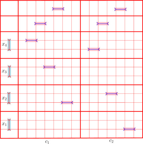
Figure 2: An example for the grid of corridors for $\Phi=(x_{2}\vee\overline{x}_{3}\vee\overline{x}_{4})\wedge(x_{1}\vee\overline{x}_{2}\vee x_{4})$ (in red). The clause gadgets (five gadgets per clause) are in shaded pink. The side corridors are not shown; they are detailed in Fig. 4.

Each $1\times 2$ (resp., $2\times 1$) room in the proof of Theorem 1 is replaced by a concentric $(1+2a)\times(2a)$ (resp., $(2a)\times(1+2a)$) bounding box $b$, where $a=0.05$. See Fig. 3. These bounding boxes are not contained in the polygon; in each bounding box, $P$ contains a unit-length axis-parallel corridor and four spikes that connect the four corners of the bounding box to the unit segment (in particular, the diameter of the unit segment and the four spikes is ${\rm diam}(b)$).

Let the diameter threshold be $\delta:=1.103$, where ${\rm diam}(b)=\sqrt{(1+2a)^{2}+(2a)^{2}}=\sqrt{1.22}>1.104$. Each box $b$ can be split into pieces of diameter less than $\delta$ by a laser along a grid line passing through $b$. Therefore, we can prove the correctness of the reduction similarly to the proof of Theorem 1. However, we need to control how the grid is subdivided into pieces of diameter at most $\delta$ (independent of the truth assignment of the variables). This is the primary role of the side-corridors that we discuss in the remainder of the proof.

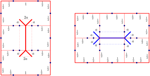
Figure 3: A variable gadget (left) and a clause gadget (right), with four spikes of length $\sqrt{2}a$. Each dot indicates a pair of doors on opposite sides of corridors, which are shown in detail in Fig. 4.

We attach a set $\mathcal{S}$ of side-corridors to the grid as follows:

1. For every $s\in\mathcal{S}$, ${\rm diam}(s)=\sqrt{5/4}\approx 1.118>\delta$, hence $s$ requires at least one laser.

2. Every $s\in\mathcal{S}$ is connected the grid by a very short and narrow corridor, called the door of $s$; a laser through this door can split $s$ into two pieces of diameter less than $\delta$.

3. $\mathcal{S}$ is partitioned into pairs $\{s_{1},s_{2}\}\subset\mathcal{S}$ such that the doors of $s_{1}$ and $s_{2}$ are located symmetrically on opposite sides of a grid corridor, and a laser can split both $s_{1}$ and $s_{2}$ into pieces of diameter at most $\delta$ iff $\{s_{1},s_{2}\}$ is a pair. (Fig. 4(middle)–(right) show side-corridors in two adjacent grid cells on opposite sides of a corridor.)

4. Therefore, every optimal solution contains a laser for each pair of side-corridors in $\mathcal{S}$.

5. There is a pair of doors at every intersection between a main corridor (of the grid) and the bounding box of a gadget.

6. The number $k$ of lasers equals $n+2m$ (one per variable gadget, two per clause gadget) plus half the number of side-corridors, which is proportional to the total length $O(mn)$ of the grid.

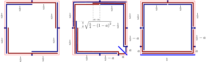
Figure 4: Side-corridors for three types of holes of the grid. Left: A hole not adjacent to any gadget. Middle: a hole adjacent to a corner of a gadget (with a spike in the lower right corner). Right: a hole adjacent to the side of a gadget (the unit-length corridor of a gadget is the bottom edge, highlighted in blue).

Figure 3 indicates the locations of the doors to matching pairs of side-corridors in a grid; and Figure 4 shows the specific shapes of these side-corridors in a grid cell. Lasers placed at every pair of side-corridors decompose the polygon into cells of diameter at most $\delta$, and the bounding boxes of the gadgets boxes. It follows that the reduction in the proof of Theorem 1 goes though, the decision problem whether $P$ can be subdivided into pieces of diameter $\delta$ with a given number of lasers is NP-hard. ∎

3 Decomposition Algorithms for Simple Polygons

In this section, we present approximation results for decomposing a simple polygon $P$ by lasers of arbitrary orientations (recall that $n$ denotes the total number of vertices of $P$ and $r$ is the number of reflex vertices). We describe an $O(\log r)$-approximation for Min-LaserArea (Section 3.1), a bi-criteria algorithm for diameter (Section 4.1), and a $O(1)$-approximation for MinDiameter (Section 4.2).

3.1 Min-LaserArea

Given a simple polygon $P$ and a threshold $\delta$, we wish to find the minimum number of lasers that subdivide $P$ into pieces, each of area at most 1. We start with the easy $O(1)$-approximation in the special case when $P$ is a convex polygon.

Lemma 4.

For every convex polygon $P$, we can find a set of $k=O(\sqrt{{\rm area}(P)})$ lasers that subdivide $P$ into pieces, each of area at most 1, in $O(k+n)$ time. Every decomposition into pieces of area at most 1 requires $\Omega(\sqrt{{\rm area}(P)})$ lasers.

Proof.

For the lower bound, notice that the arrangement of $\ell$ lines has $O(\ell^{2})$ faces, and so $\ell$ lasers decompose $P$ into $O(\ell^{2})$ cells. By the pigeonhole principle, the area of the largest piece is $\Omega({\rm area}(P)/\ell^{2})\leq 1$. Hence $\ell\geq\Omega(\sqrt{{\rm area}(P)})$, as claimed.

For the upper bound, recall that by John’s theorem [3, 21], $P$ contains an ellipse $E$ such that $E\subset P\subset 2E$, where $2E$ is obtained from $E$ by central dilation of ratio 2. Let $B$ be a bounding box of $P$ (i.e., a rectangle of arbitrary orientation that contains $P$) of minimum area. Then ${\rm area}(E)\leq{\rm area}(P)\leq{\rm area}(B)\leq\frac{4}{\pi}\,{\rm area}(2E)=O({\rm area}(E))$, hence ${\rm area}(B)\leq O({\rm area}(P))$, and $B$ can be computed in $O(n)$ time [12, 34]. Assume, w.l.o.g., that $B$ is axis-aligned with the lower-left corner at the origin. For every $m\in\mathbb{N}$, we can decompose the rectangle $B$ into $m^{2}$ congruent rectangles with $2(m-1)$ axis-parallel lasers: $m-1$ equally spaces horizontal (resp., vertical) lasers. If $m=\lceil\sqrt{{\rm area}(B)}\rceil=O(\sqrt{{\rm area}(P)})$, then the area of each piece is at most ${\rm area}(B)/m\leq 1$. These $\ell=2m-2$ lasers decompose $P$ into pieces of area at most $1$, as well, as required. ∎

Overview.

We give a brief overview of our approximation algorithm for a simple polygon $P$. The basic idea is to decompose $P$ into convex pieces, and use Lemma 4 to further decompose each convex piece. There are two problems with this naïve approach: (1) a laser in an optimal solution may intersect several convex pieces (i.e., the sum of lower bounds for the convex pieces is not a global lower bound); and (2) the lasers used for a convex decomposition are not accounted for. We modify the basic approach to address both of these problems.

We use the Hershberger–Suri triangulation (as a convex subdivision). For a simple polygon $P$ with $n$ vertices, Hershberger and Suri [19] construct a Steiner triangulation into $O(n)$ triangles such that every chord of $P$ intersects $O(\log n)$ triangles. We can modify their construction to produce a Steiner decomposition into a set $\mathcal{C}$ of convex cells (rather than triangles) such that each laser intersects $O(\log r)$ convex cells, where $r$ is the number of reflex vertices of $P$. Thus, each laser of ${\rm OPT}$ can help partition $O(\log r)$ convex cells; this factor dominates the approximation ratio of our algorithm.

A convex cell $C\in\mathcal{C}$ is large if ${\rm area}(C)>1$, otherwise it is small. We decompose each large convex cell using Lemma 4. We can afford to place $O(1)$ lasers along the boundary of a large cell. We cannot afford to place lasers on the boundaries of all small cells. If we do not separate the small cells, however, they could merge into a large (nonconvex) region, so we need some separation between them. In the algorithm below, we construct such separators recursively by carefully unrefining the Hershberger–Suri triangulation. The unrefined subdivision is no longer a triangulation, but we maintain the properties that (i) each cell is bounded by $O(1)$ lasers within each pseudotriangle (and an arbitrary number of consecutive edges of $P$), and (ii) every chord of $P$ intersects $O(\log n)$ cells.

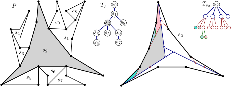
Figure 5: Left: A simple polygon $P$, decomposed into pseudotriangles, and the dual graph $T_{P}$. Right: A pseudotriangle $s_{2}$ is recursively subdivided into Steiner triangles, with recursion tree $T_{s_{2}}$.

Basic properties of the Hershberger–Suri triangulation.

Given a simple polygon $P$ with $n$ vertices, Hershberger and Suri [19] construct a Steiner-triangulation in two phases (see Fig. 5 for an example): First, they subdivide $P$ into $O(n)$ pseudotriangles (i.e., simple polygons with precisely three convex vertices) using $O(n)$ noncrossing diagonals of $P$; and then subdivide each pseudotriangle into Steiner triangles. The runtime of their algorithm, as well as the number of Steiner triangles, is $O(n)$. Let $\mathcal{S}$ denote the set of pseudotriangles produced in the first phase; and let $T_{P}$ be the dual tree of the pseudotriangles, in which each node corresponds to a pseudotriangle, and two nodes are adjacent if and only if the corresponding pseudotriangles share an edge (a diagonal of $P$). Note that the degree of $T_{P}$ is not bounded by a constant (it is bounded by $n$), as a pseudotriangle may be adjacent to arbitrarily many other pseudotriangles. We consider $T_{P}$ to be a rooted tree, rooted at an arbitrary pseudotriangle. Then every nonroot pseudotriangle $s$ in $\mathcal{S}$ has a unique edge incident to the parent of $s$; we call this edge the parent edge of $s$.

Hershberger and Suri subdivide each pseudotriangle $s\in S$ recursively: In each step, they use $O(1)$ line segments to subdivide a pseudotriangle into $O(1)$ pseudotriangles, which are further subdivided recursively until they obtain triangles. Let us denote by $T_{s}$ the recursion tree for $s$. Each vertex $v\in T_{s}$ represents a region $R_{v}\subset s$: The root of $T_{s}$ represents $s$, and the leaves represent the Steiner triangles in $s$. The recursive subdivision maintains the following two properties: (a) Every edge of $s$ is incident to a unique region in each level of $T_{s}$, (b) For each node $v\in T_{s}$, the boundary between $R_{v}$ and $s\setminus R_{v}$ is a polyline with $O(1)$ edges (that is, $R_{v}$ is bounded by $O(1)$ line segments inside $s$, and some sequence of consecutive edges of $s$).

Algorithm. We are ready to present an approximation algorithm for Min-LaserArea. Given a simple polygon $Q$, we begin by computing the Hershberger–Suri triangulation, the pseudotriangles $\mathcal{S}$, the dual tree $T_{P}$, and a recursion tree $T_{s}$ for each pseudotriangle $s\in\mathcal{S}$. We then process the pseudotriangles in a bottom-up traversal of $T_{P}$.

Within each pseudotriangle $s\in\mathcal{S}$, we unrefine the Steiner triangulation of $s$ by merging some of the cells into one cell (the resulting larger cells need not be triangular or convex). Initially, each node $v\in T_{s}$ corresponds to a region $R_{v}\subseteq s$. However, if we do not place lasers along the edges of $s$, then $R_{v}$ may be adjacent to (and merged with) other cells that are outside the pseudotriangle $s$, along the boundary of $s$. Since we have an upper bound on the total area of each cell in the final decomposition, we need to keep track of the area of the region on both sides of an edge of the pseudo-triangulation. In the course of unrefinement algorithm for all $s\in\mathcal{S}$, we compute nonnegative weights $w(\cdot)$ for all edges of the pseudotriangulation. The weights are used for bookkeeping purposes. Specifically, the edges of $P$ have zero weight. In a bottom-up traversal of $T_{P}$, when we start processing a pseudotriangle $s$, the weights $w(e)$ have already been computed for all edges of the pseudo-triangle $s$ except the parent edge of $s$. The weight $w(e)$ for the parent edge $e$ of $s$ is determined when we have computed the unrefined subdivision of $s$; and $w(e)$ will be the area of the unrefined cell in $s$ adjacent to the parent edge. A node $v\in T_{s}$ initially corresponds to a region $R_{v}$ within the pseudotriangle $s$, but in the final decomposition of $P$, the node is part of some larger cell $\widehat{R}_{v}\subseteq P$, with ${\rm area}(\widehat{R}_{v})={\rm area}(R_{v})+\sum_{e}w(e)$, where the summation is over all edges of $s$ on the boundary of $R_{v}$, and $w(e)$ denotes the area of the cell on the opposite side of $e$.

As the weight of the parent edge is not available yet when we unrefine $s$, we modify the recursion tree $T_{s}$ as follows: We choose the root to be the leaf $v_{0}\in T_{s}$ adjacent to the parent edge of $s$, and reverse the parent-child relation on all edges of $T_{s}$ along the $s$-$v_{0}$ path. We denote the modified recursion tree $T^{\prime}_{s}$ (Fig. 6 (left)). For all nodes $v$ along the $s$-$v_{0}$ path (including $s$ and $v_{0}$), we redefine the corresponding regions of the nodes in $T^{\prime}_{s}$ as follows. We denote by $R_{v}(T_{s})$ and $R_{v}(T^{\prime}_{s})$ the regions corresponding to node $v$ in trees $T_{s}$ and $T^{\prime}_{s}$, respectively. We set $R_{v_{0}}(T^{\prime}_{s}):=s$ and for all other nodes $v$ along the $s$-$v_{0}$ path (including $s$), we set $R_{v}(T^{\prime}_{s}):=s\setminus R_{u}(T_{s})$, where $u$ is the parent of $v$ in $T^{\prime}_{s}$. With a slight abuse of notation, we set $R_{v}=R_{v}(T^{\prime}_{s})$ for all $v\in T^{\prime}_{s}$ for the remainder of the algorithm. Note that ${\rm area}(R_{v})$ monotonically decreases with the depth in $T^{\prime}_{S}$.

In a bottom-up traversal of $T_{P}$, consider every $s\in\mathcal{S}$. We proceed with two phases (see Fig. 6 for an example).

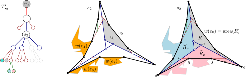
Figure 6: Left: The modified recursion tree $T_{s_{2}}^{\prime}$. Middle: pseudotriangle $s_{2}$ with the initial Steiner triangulation, edge weights representing the areas of adjacent regions in the descendants of $s_{2}$, and the parent edge $e_{0}$ of $s_{2}$. Right: The unrefined subdivision of $s_{2}$ into $R_{u}$, $R_{v}$, and $R$; larger cells $\widehat{R}_{u}$ and $\widehat{R}_{v}$ (blue and pink), and the weight $w(e_{0})={\rm area}(R)$ of the parent edge of $s_{2}$ (gray).

Phase 1 of the algorithm is an unrefinement process, that successively merges small cells of the Hershberger–Suri triangulation (no lasers are involved). We initialize three variables:

$$R:=s,\hskip 17.07164ptT:=T^{\prime}_{s},\hskip 17.07164ptU_{s}:=\emptyset,$$

where $R\subseteq s$ is the region yet to be handled, $T$ is a subtree of $T_{s}^{\prime}$ corresponding to the region $R$, and $U_{s}$ is the set of interior-disjoint faces in $s$ produced by the unrefinement process. While ${\rm area}(R)>1$, do the following:

• Find a lowest node $v\in T$ for which ${\rm area}(\widehat{R}_{v})>1$,

• Set $U_{s}:=U_{s}\cup\{\widehat{R}_{v}\}$,

• Set $R:=R\setminus R_{v}$,

• Delete the subtree rooted at $v$ from $T$, and

• For all ancestors $u$ of $v$, set $\widehat{R}_{u}:=\widehat{R}_{u}\setminus\widehat{R}_{v}$.

When the while loop ends, define the weight of the parent edge of $s$ to be ${\rm area}(R)$.

Phase 2 of the algorithm positions lasers in a pseudotriangle $s$ as follows.
For every region $\widehat{R}_{v}\in U_{s}$, do:

• Step 1. Place lasers along all edges of the boundary between $\widehat{R}_{v}$ and $s\setminus\widehat{R}_{v}$, and the boundaries between $R_{v}$ and $R_{v^{\prime}}$ for all children $v^{\prime}$ of $v$. For example in Fig. 6 (right), two lasers are placed along the edges $(a,c)$ and $(c,e)$ that disconnect $\widehat{R}_{v}$ from $s_{2}$. Also, a laser that is placed along edge $(b,d)$ that separates the children of $R_{v}$.

• Step 2. If ${\rm area}(R_{v})\geq 1$ (which means $R_{v}$ has not merged with any other region in Phase 1, i.e., $\widehat{R}_{v}=R_{v}$ hence $\widehat{R}_{v}$ is convex), subdivide $\widehat{R}_{v}$ by $\Theta(\sqrt{{\rm area}(R_{v})})$ lasers according to Lemma 4.

This completes the description of our algorithm.

Theorem 5.

Let $P$ be a simple polygon with $n$ vertices, and let $k^{*}$ be the minimum number of lasers that subdivide $P$ into pieces of area at most $1$. We can find an integer $k$ with $k^{*}\leq k\leq O(k^{*}\log n)$ in $O(n)$ time, and a set of $k$ lasers that subdivide $P$ into pieces of area at most $1$ in output-sensitive $O(k+n)$ time.

Proof.

Phase 1 of our algorithm (unrefinement) subdivides each pseudotriangle $s\in\mathcal{S}$ into regions such that each region corresponds to a subtree rooted at some node $v$ of the recursion tree $T_{s}^{\prime}$. Node $v$ corresponds to a region $R_{v}\subset s$, and a possibly larger region $\widehat{R}_{v}\subset P$ which is the union of $R_{v}$ and adjacent regions in the descendant pseudotriangles of $s$ adjacent to $R_{v}$. Phase 1 of the algorithm ensures that ${\rm area}(\widehat{R}_{v})>1$ (therefore, $\widehat{R}_{v}$ must intersect at least one laser in ${\rm OPT}$), but for all children $v^{\prime}$ of $v$ in $T^{\prime}_{s}$, we have ${\rm area}(\widehat{R}_{v^{\prime}})\leq 1$.

In Step 1, the algorithm uses $O(1)$ lasers for each $v\in U_{s}$ to separate $\widehat{R}_{v}$ from $s\setminus\widehat{R}_{v}$. Recall that the recursion tree $T_{s}$ has bounded degree. Consequently, we use $O(1)$ lasers to separate $\widehat{R}_{v^{\prime}}$ from $\widehat{R}_{v}\setminus\widehat{R}_{v^{\prime}}$ for all children $v^{\prime}$ of $v$. These polylines subdivide $\widehat{R}_{v^{\prime}}$ into smaller regions of area at most $1$. Overall, we have used $O(1)$ lasers for each of these nodes $v\in T_{s}^{\prime}$, $s\in\mathcal{S}$. Note that each region $\widehat{R}_{v}$ is the union of triangles from the Hershberger–Suri Steiner triangulation, and so each laser in ${\rm OPT}$ intersects $O(\log n)$ such regions. Consequently, we use $O(k^{*}\,\log n)$ lasers in Step 1.

Finally, consider the lasers used in Step 2 for subdividing the triangles $t\in T$ with ${\rm area}(t)>1$. By Lemma 4, each such triangle intersects at least $\Omega(\sqrt{{\rm area}(t)})$ lasers in any valid solution; and conversely each laser of an optimal solution intersects $O(\log n)$ regions in $T$. Consequently, the number of lasers uses in Step 2 is $\sum_{t\in T}O(\sqrt{{\rm area}(t)})\leq O(k^{*}\,\log n)$.

It remains to show that the algorithm runs in $O(n+k)$ time. The Hershberger-Suri Steiner triangulation can be computed in $O(n)$ time [19]. It consists of $O(n)$ triangles, hence the combined size of the dual tree $T_{p}$, and the recursion trees $T_{s}$, $s\in\mathcal{S}$, is also $O(n)$. The unrefinement algorithm is done in a single traversal of these trees, spending $O(1)$ time at each node. For each large cell (triangle) of the Hershberger-Suri triangulation, by Lemma 4, we can compute a minimum bounding box and the number of lasers used by the algorithm in $O(1)$ time. Computing all $k$ lasers requires $O(k)$ additional time. ∎

An $O(\log r)$ Approximation for Min-LaserArea in Simple Polygons.

We can improve the approximation ratio in Theorem 5 from $O(\log n)$ to $O(\log r)$, where $r$ is the number of reflex vertices of $P$, if we replace the Hershberger–Suri triangulation with a convex decomposition. (Hershberger and Suri decompose $P$ into triangles to support ray shooting queries, but for our purposes a decomposition into convex cells suffices.)

Let $(v_{1},\ldots,v_{n})$ be the $n$ vertices of $P$; assume they are in general position. Let $R$ be the set of reflex vertices of $P$. For every reflex vertex $v\in R$, the angle bisector of the interior angle at $v$ hits some edge $a_{v}b_{v}$ of $P$. Let $L=\{v,a_{v},b_{v}:v\in R\}$, that is, $L$ is the set of all reflex vertices of $P$, and both endpoints of the edges hit by the angle bisectors of reflex angles. Clearly, $|L|\leq 3r$.

Lemma 6.

There is a simple polygon $Q\subset P$ whose vertex set is $L$, and every connected component of $P\setminus Q$ is a convex polygon. The polygon $Q$ can be computed in $O(n\log n)$ time.

Proof.

We describe an algorithm that decomposes $P$ along noncrossing diagonals into a collection $\mathcal{P}$ of convex polygons and their complement $P\setminus(\bigcup_{A\in\mathcal{P}}A)$ will be polygon $Q$. Initially $\mathcal{P}=\{P\}$ and $Q=\emptyset$.

The algorithm has two steps. In the first step, a collection $\mathcal{P}$ of convex polygons is created such that the vertex set of the complement $P\setminus(\bigcup_{A\in\mathcal{P}}A)$ is $L$. However, $P\setminus(\bigcup_{A\in\mathcal{P}}A)$ is not necessarily connected. In the second step, the connected components of $P\setminus(\bigcup_{A\in\mathcal{P}}A)$ are merged into a simple polygon $Q$ (a single connected component) with the same vertex set $L$.

First step:

While there is a nonconvex polygon $P^{\prime}\in\mathcal{P}$, we replace $P^{\prime}$ with one or more smaller polygons in $\mathcal{P}$ as follows. Let $v$ be a reflex vertex of $P^{\prime}$. Since $P^{\prime}\subset P$, vertex $v$ is also a reflex vertex of $P$. Denote by $\vec{r}_{v}$ the angle bisector of $P$ at $v$. Note that $\vec{r}_{v}$ enters the interior of $P^{\prime}$ at $v$; denote by $ab$ the edge of $P^{\prime}$ where $\vec{r}_{v}$ first exits $P^{\prime}$. Let $P(v)$ be the geodesic triangle formed by the edge $ab$ and the shortest paths from $v$ to $a$ and to $b$, respectively. Update $\mathcal{P}$ by replacing $P^{\prime}$ with the polygons in $P^{\prime}\setminus P(v)$. See Figure 7 for an example. In the course of the algorithm, every polygon in $\mathcal{P}$ is formed by a sequence of consecutive vertices of the input polygon $P$.

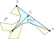
Figure 7: Replace $P^{\prime}$ by four polygons (in yellow), after taking out the geodesic triangle $P(v)$ where $v$ is a reflex vertex.

We claim that in each iteration of the algorithm, all vertices of $P(v)$ are in $L$. Clearly, $v$ is a reflex vertex in $P^{\prime}$, hence a reflex vertex of $P$, as well. Similarly, the interior vertices of the shortest paths from $v$ to $a$ and to $b$ are reflex vertices in $P^{\prime}$, hence in $P$. It remains to show that $a,b\in L$. If $ab$ is an edge of $P$, then $a,b\in L$ by the definition of $L$. Otherwise, $ab$ is a diagonal of $P$, and so it is an edge of a geodesic triangle $P(v^{\prime})$ of some previous iteration of the algorithm—by induction, they are in $L$, as well. At the end of the while loop, all polygons in $\mathcal{P}$ are convex, however, the complement $P\setminus(\bigcup_{A\in\mathcal{P}}A)$ is not necessarily connected. See Figure 8 for an illustration.

Figure 8: A simple polygon $P$, the vertices in $L$ are blue (reflex) or red (hit by angle bisector). Left: The first step produces convex polygons $\mathcal{P}=\{A_{1},\ldots,A_{6}\}$, but $P\setminus\bigcup_{i=1}^{6}A_{i}$ is disconnected. Right: The second step merges $P\setminus\bigcup_{i=1}^{6}A_{i}$ into a simple polygon $Q$. As $|A_{3}\cap L|\geq 3$ and $|A_{4}\cap L|\geq 3$, the second step creates conv$(V(A_{3})\cap L)$ and conv$(V(A_{4})\cap L)$ (shown in deep yellow) which merges $P\setminus\bigcup_{i=1}^{6}A_{i}$ into a single connected component $Q$.

Second step:

While there is a (convex) polygon $P^{\prime}\in\mathcal{P}$ incident to three or more vertices in $L$, we replace $P^{\prime}$ with smaller polygons: In particular, let $V(P^{\prime})$ be the vertex set of $P^{\prime}$. If $|V(P^{\prime})\cap L|\geq 3$, then replace $P^{\prime}$ with the polygons in $P^{\prime}\setminus\text{conv}(V(P^{\prime})\cap L)$, where $\text{conv}(.)$ stands for the convex hull. In each iteration, all polygons in $\mathcal{P}$ remain convex. At the end of the while loop, every polygon in $\mathcal{P}$ is incident to exactly two vertices in $L$, and $P\setminus(\bigcup_{A\in\mathcal{P}}A)$ is a simple polygon with vertex set $L$. ∎

Lemma 7.

Every simple polygon $P$ on $n$ vertices, $r$ of which are reflex, can be decomposed into convex faces such that every chord of $P$ intersects $O(\log r)$ faces. Such a decomposition can be computed in $O(n\log n)$ time.

Proof.

We can compute the set $L$ of up to $3r$ vertices and a simple polygon $Q\subset P$ described in Lemma 6 in $O(n\log n)$ time. We then compute the Hershberger–Suri triangulation for $Q$, which is a Steiner triangulation of $O(r)$ triangles such that every chord of $Q$ intersects $O(\log r)$ triangles [19]. This triangulation of $Q$, together with the convex polygons in $P\setminus Q$, form a subdivision of $P$ into convex faces.

We claim that every chord of $P$ intersects at most $O(\log r)$ faces: at most $O(\log r)$ triangles in $Q$ and at most two convex sets in $P\setminus Q$. If a chord $\ell$ of $P$ intersects three components of $P\setminus Q$, say $C_{1},C_{2},C_{3}$ in this order, then $\ell$ crosses the boundary of $C_{2}$ twice, so $C_{2}$ must have at least two edges on the boundary between $C_{2}$ and $Q$. However, by Lemma 6, every edge of $Q$ is either an edge or a diagonal of $P$. Therefore the boundary between $Q$ and a component of $P\setminus Q$ is a single diagonal of $P$. Thus $\ell$ intersects at most two components of $P\setminus Q$; moreover $\ell\cap Q$ is a chord of $Q$, so it intersects $O(\log r)$ triangles inside $Q$. ∎

By performing the algorithm on the convex subdivision in Corollary 7, the approximation ratio improves to $O(\log r)$.

Theorem 8.

Let $P$ be a simple polygon with $n$ vertices, $r$ of which are reflex, and let $k^{*}$ be the minimum number of lasers needed to subdivide $P$ into pieces of area at most $1$. We can find an integer $k$ with $k^{*}\leq k\leq O(k^{*}\log r)$ in $O(n\log n)$ time, and a set of $k$ lasers that subdivide $P$ into pieces of area at most $1$ in output-sensitive $O(k+n\log n)$ time.

4 Diameter in simple polygons

4.1 Bi-Criteria Approximation for Diameter

For the diameter version in a simple polygon, we describe a bi-criteria approximation algorithm (Theorem 11). We start from deriving a lower bound for the minimum number of lasers in a decomposition into pieces of diameter at most $\delta$ (for bi-criteria approximation algorithm we use general $\delta$, instead of $\delta$ =1, because we will scroll over $\delta$ when using the algorithm to get an approximation for MinDiameter).

Consider the infinite set of vertical lines, $\mathcal{L}_{V}$, evenly spaced with separation $\delta$; that is, $\mathcal{L}_{V}=\{x=i\delta:i\in\mathbb{Z}\}$. The lines in $\mathcal{L}_{V}$ decompose $P$ into a set $\mathcal{P}_{V}$ of simple polygons, that we call cells. By construction, the orthogonal projection of each cell to the $x$-axis is an interval of length at most $\delta$. (More precisely, we consider the polygon $P$ to be a closed set in the plane. Subtracting the union of vertical lines $\mathcal{L}_{V}$ from $P$ results in a set of connected components; the closures of these components are the simple polygons in $\mathcal{P}_{V}$). The polygons in $\mathcal{P}_{V}$ are faces in the arrangement of the lines in $\mathcal{L}_{V}$ and the edges of $P$; the planar dual of this decomposition is a tree, whose nodes are the faces $\mathcal{P}_{V}$ and whose edges are dual to the vertical lines.

If the projection of polygon $Q\in\mathcal{P}_{V}$ onto the $x$-axis is an interval of length $\delta$ (which means it extends from $x=i\delta$ to $x=(i+1)\delta$, for some integer $i$), we say that $Q$ is a full-width cell; otherwise the projection of $Q$ onto the $x$-axis is of length less than $\delta$, and we say that $Q$ is a narrow cell. (It may be that $P$ itself is a narrow cell if, e.g., $P$ does not intersect any of the vertical lines $L_{V}$.)

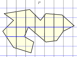
Figure 9: $P$ is subdivided by a grid; the lasers are thick

The intersection of the lines in $\mathcal{L}_{V}$ with $P$ is a set of vertical chords of $P$. Let $C_{V}$ be the set of these chords. While there is a chord $\ell\in C_{V}$ that lies on the boundary of some narrow cell, remove $\ell$ from $C_{V}$ (thereby merging the cells on the two sides of $\ell$ into one cell). As a result, all remaining chords lie on the boundary between full-width cells. Let $C_{V}^{\prime}$ be the resulting set of chords, and let $k_{V}=|C_{V}^{\prime}|$ denote their cardinality. Since any two full-width cells of $\mathcal{P}_{V}$ that are in adjacent vertical strips remain separated by a chord in $C_{V}^{\prime}$, the $x$-extent of each face in the new decomposition of $P$ is at most $3\delta$. We summarize this below.

Proposition 9.

The remaining $k_{V}$ chords $C_{V}^{\prime}$, $k_{V}\geq 0$, subdivide $P$ into a set $\mathcal{Q}$ of $k_{V}+1$ polygons, each of which intersects at most two lines in $\mathcal{L}_{V}$, consequently its projection to the $x$-axis is an interval of length less than $3\delta$. Further, the dual graph of this decomposition is a tree (with $k_{V}$ edges and $k_{V}+1$ nodes).

If $k_{V}=0$, then there is just one cell, $\mathcal{Q}=\{P\}$. If $k_{V}\geq 1$, then each $Q\in\mathcal{Q}$ includes at least one full-width cell, since the only lasers remaining are those separating one full-width cell from an adjacent full-width cell sharing the laser.

Thus, the boundary of each $Q\in\mathcal{Q}$ includes at least two distinct (simple) paths connecting a point on one line of $\mathcal{L}_{V}$ to a point on an adjacent line of $\mathcal{L}_{V}$. Each of these paths has length at least $\delta$. The endpoints of such a path are at distance at least $\delta$ away from each other. In any laser cutting of $P$ into pieces of diameter at most $\delta$, each such path contains a laser endpoint in its interior or at both endpoints (if the path is a horizontal line segment). In any case, each of these paths contains a laser endpoint in its interior or at its left endpoint. Thus overall, there must be at least $2|\mathcal{Q}|=2(k_{V}+1)$ endpoints of lasers. This implies that $k^{*}\geq k_{V}+1$, where $k^{*}$ is the minimum number of lasers in order to achieve pieces of diameter at most $\delta$. Therefore we conclude,

Lemma 10.

If $k_{V}\geq 1$, then $k^{*}\geq k_{V}+1$.

Now, we consider the set of horizontal lines, $\mathcal{L}_{H}=\{y=j\delta:j\in\mathbb{Z}\}$, and apply the above process to polygon $P$, yielding horizontal chords $C_{H}$, and then a subset $C_{H}^{\prime}\subseteq C_{H}$ of chords after merging cells (removing lasers that separate a full-height cell from an adjacent short cell). The result is a decomposition of $P$ into $k_{H}+1=|C_{H}^{\prime}|+1$ pieces, each having projection onto the $y$-axis of length less than $3\delta$. Analogously to Lemma 10, we get $k^{*}\geq k_{H}+1$ if $k_{H}\geq 1$.

If we now overlay the vertical chords $C_{V}^{\prime}$ and the horizontal chords $C_{H}^{\prime}$, the resulting arrangement decomposes $P$ into pieces each of which is a simple polygon having projections onto both the $x$- and the $y$-axis of lengths less than $3\delta$; thus, the resulting pieces each have diameter less than $3\delta\sqrt{2}$. The total number of lasers is $k_{V}+k_{H}\leq 2(k^{*}-1)$.

Theorem 11.

Let $P$ be a simple polygon with $n$ vertices, and let $k^{*}$ be the minimum number of lasers that decompose $P$ into pieces each of diameter at most $\delta$ for a fixed $\delta>0$. One can compute a set of at most $2(k^{*}-1)$ axis-aligned lasers that decompose $P$ into pieces each of diameter at most $3\sqrt{2}\delta$ in time polynomial in $n$ and ${\rm diam}(P)/\delta$.

4.2 $O(1)$-Approximation for MinDiameter in simple polygons

In this section we consider the problem of minimizing the maximum diameter of a cell in the arrangement of $k$ lasers, for a given number $k$. Our $O(1)$-approximation algorithm repeatedly decreases the $x$- and $y$- separation in the bi-criteria solution from Theorem 11 until the number of placed lasers is about to jump over 2$k$; then, the number of lasers is halved while increasing the diameter by a constant factor.

Specifically, let $\ell(\delta)$ denote the number of lasers used in the end of the bi-criteria algorithm with the $x$- and $y$-separation between consecutive vertical and horizontal lines being $\delta$. Our algorithm to approximate the diameter achievable with $k$ lasers is as follows:

• Initialize $\delta={\rm diam}(P)$, and $\varepsilon>0$

• While $\ell(\delta)\leq 2k$, set $\delta=\delta/(1+\varepsilon)$ and recompute $\ell(\delta)$.

• Let $\delta_{0}$ be such that $\ell(\delta_{0})\leq 2k$ but $\ell(\delta_{0}/(1+\varepsilon))>2k$.

• Let $C_{V}$ and $C_{H}$ be the $\ell(\delta_{0})\leq 2k$ vertical and horizontal lasers, resp., found by the bi-criteria algorithm.

• Partition $C_{V}$ into lasers along $x=i\delta_{0}$ for even $i$ and the rest (odd $i$); let $C_{V}^{\prime}$ be a smallest part. Similarly, let $C_{H}$ be a smaller part when we partition $C_{H}$ into two subsets of lines where $y=i\delta_{0}$ is an even or odd multiple of $\delta_{0}$.

• Return the lasers in $C_{V}^{\prime}\cup C_{H}^{\prime}$.

Theorem 12.

Let $P$ be a simple polygon with $n$ vertices, and let $\delta^{*}$ be the optimal diameter achievable with $k$ lasers. For every $\varepsilon>0$, one can compute a set of at most $k$ lasers that partition $P$ into pieces each of diameter at most $4\sqrt{2}(1+\varepsilon)\delta^{*}$ in time polynomial in $n$, ${\rm diam}(P)/\delta^{*}$, and $\varepsilon$.

Proof.

By Theorem 11, if $\delta^{*}$ were smaller than $\delta_{0}/(1+\varepsilon)$, then $\ell(\delta_{0}/(1+\varepsilon))$ would have been at most $2k$, which is not the case (by the choice of $\delta_{0}$), implying that $\delta^{*}\geq\delta_{0}/(1+\varepsilon)$. Our algorithm starts with at most $2k$ lasers, produced by the bi-criteria solution, that decomposes $P$ into pieces that each intersects at most two consecutive lines in $L_{V}=\{x=i\delta_{0}:i\in\mathbb{Z}\}$ and $L_{H}=\{y=i\delta_{0}:i\in\mathbb{Z}\}$, hence their $x$- and $y$-projections have length at most $3\delta_{0}$. By removing at least half of the horizontal (resp., vertical) lasers, the number of lasers drops to $k$ or below, and the pieces on opposite sides of these lasers merge. The removal of a laser along a line $x=i\delta_{0}$ creates a piece that can intersect only $x=j\delta_{0}$ for $j\in\{i-1,i,i+1\}$. Therefore, each resulting piece intersects at most 3 consecutive lines in $L_{V}$ and $L_{H}$, respectively, they each have $x$- and $y$-projection of length at most $4\delta_{0}$. Hence the diameter of the final pieces is at most $4\sqrt{2}\delta_{0}\leq 4\sqrt{2}(1+\varepsilon)\delta^{*}$. ∎

5 Axis-Parallel Lasers

In this section we study Min-LaserDiameter and Min-LaserArea under the constraint that all lasers must be axis-parallel (the edges of $P$ may have arbitrary orientations). The algorithms for both problems start with a “window partitioning” $P$ into “(pseudo-)histograms” of stabbing number at most three, and are then tuned to the specific measures to partition the histograms. We use a simple sweepline algorithm for the diameter, and a dynamic program for the area. The main result is:

Theorem 13.

Let $P$ be a simple polygon with $n$ vertices and let $k^{*}$ be the minimum number of axis-parallel lasers needed to subdivide $P$ into pieces of area (diameter) at most $1$. There is an algorithm that finds $O(k^{*})$ axis-parallel lasers that subdivide $P$ into pieces of area (diameter) at most $1$ in time polynomial in $n$ and ${\rm area}(P)$ (${\rm diam}(P)$).

5.1 Reduction to Histograms

A histogram is a simple polygon bounded by an axis-parallel line segment, the base, and an $x$- or $y$-monotone polygonal chain between the endpoints of the base.

The window partition of a simple polygon was originally used for the design of data structures that support link distance queries [27, 33]. In this section, we use the axis-parallel version, which partitions a simple polygon $P$ into histograms such that every axis-parallel chord of $P$ intersects at most 3 histograms. Window partitions for orthogonal polygons can be computed by a standard recursion [27, 33]; we use a modified version where we recurse until the remaining subpolygons are below the size threshold $1$. This modification guarantees termination on all simple polygons (not only orthogonal polygons).

Figure 10: Window partition of a polygon $Q$ with a horizontal base $b$ into a maximal histogram $H$ (colored gold) and four polygons $Q_{1}$, $Q_{2}$, $Q_{3}$, and $Q_{4}$ (in white). If the sizes (areas/diameters) of $Q_{1}$, $Q_{2}$, $Q_{3}$, and $Q_{4}$ are each at most $1$, then $Q$ is a pseudo-histogram.

Window Partition Algorithm. Given a simple polygon $P$, let $b$ be an axis-parallel chord of $P$ that subdivides $P$ into two simple polygons $P_{1}$ and $P_{2}$ with a common base $b$. Let $\mathcal{S}=\{(P_{1},b),(P_{2},b)\}$ be a set of tuples where each tuple has a polygon and its axis-parallel base, and let $\mathcal{H}=\emptyset$ be the set of histograms. While $\mathcal{S}$ contains a pair $(Q,b)$, where the size (e.g., the diameter) of $Q$ is more than 1, do the following:

1. compute the maximal histogram $H$ of base $b$ in $Q$, and add $(H,b)$ to $\mathcal{H}$; See Figure 10.

2. update $\mathcal{S}$ by replacing $(Q,b)$ with the pairs $(Q_{i},b_{i})$, where the polygons $Q_{i}$ are the connected components of $Q\setminus H$, and $b_{i}$ is the boundary between $Q_{i}$ and $H$.

Return $\mathcal{H}$ and $\mathcal{S}$.

Pseudo-histograms.

Let $T_{1}$ and $T_{2}$ be the recursion trees of the algorithm, rooted at $P_{1}$ and $P_{2}$, respectively. Let $T=T_{1}\cup T_{2}$. Each node $v\in T$ corresponds to a polygon $Q_{v}\subset P$. Every nonleaf node $v\in T$ also corresponds to a histogram $H_{v}\subset Q_{v}$; it is possible that size$(H_{v})\leq 1$ but size$(Q_{v})>1$ (the size is ${\rm area}$ or ${\rm diam}$ based on the problem). For a leaf $v\in T$, we have either size$(Q_{v})\leq 1$, or $H_{v}=Q_{v}$ and size$(H_{v})>1$. The polygons $Q_{v}$ at leaf nodes and the histograms $H_{v}$ at nonleaf nodes jointly form a subdivision of $P$.

Every node $v\in T$ in the recursion tree corresponds to a polygon-base pair $(Q_{v},b_{v})$. For any subset $U\subset V(T)$, where $V(T)$ is the set of vertices of $T$, the bases $\{b_{u}:u\in U\}$ decompose $P$ into simply connected cells. For every $u\in U$, there is a cell $P_{u}$ in the decomposition such that $H_{u}\subset P_{u}\subset Q_{u}$. Since every axis-parallel chord of $P$ crosses at most 2 bases, it can intersect at most 3 polygons in such a decomposition.

In a bottom-up traversal of $T$, we can find a subset $U\subset V(T)$ such that $\{b_{u}:u\in U\}$ decomposes $P$ into polygons $P_{u}$, $u\in U$, such that size$(P_{u})>1$ but the size of every component of $P_{u}\setminus H_{u}$ is at most $1$. Each polygon $P_{u}$ consists of a histogram $H_{u}$ with base $b_{u}$, and subpolygons (pockets) of size at most 1 attached to some edges of $H_{u}$ orthogonal to $b_{u}$. We call each such polygon $P_{u}$ a pseudo-histogram. See Figure 10.

5.2 $O(1)$-Approximation for Min-LaserDiameter in Histograms

We start with an $O(1)$-approximation for histograms, and then extend our algorithm to pseudo-histograms and simple polygons. Without loss of generality, we assume that the base is horizontal.

Figure 11: Left: A histogram polygon with a horizontal base. Right: lasers introduced in Phase 1 are shown in black. Horizontal (vertical) lasers introduced in Phase 2 are shown in blue (red).

Theorem 14.

There is an algorithm that, given a histogram $P$ with $n$ vertices, computes an $O(1)$-approximation for the axis-parallel Min-LaserDiameter problem in time polynomial in $n$ and ${\rm diam}(P)$.

Proof.

We first describe the algorithm.

Algorithm. We are given a histogram $P$ with a horizontal base $ab$. If ${\rm diam}(P)\leq 1$, halt. Otherwise, do the following:

1. Subdivide $ab$ into $\lceil 2|ab|\rceil$ intervals which all, except possibly one, have length $1/2$ and place vertical lasers on the boundary between consecutive intervals.

2. Sweep $P$ with a horizontal line $L$ top down, and maintain the set of cells formed by all lasers in step one and the line $L$. When the diameter of a cell $C$ above $L$ is precisely $1$, place a horizontal laser $pq$ along the bottom side of $C$, where $p,q\in\partial P$, and place two vertical lasers at $p$ and $q$, respectively.

Analysis. Let ${\rm OPT}$ denote the set of lasers in an optimal solution, and let $k^{*}=|{\rm OPT}|$. Denote by ${\rm ALG}$ the set of lasers computed by the algorithm; let ${\rm ALG}^{1}$ be the number of vertical lasers computed in Phase 1, and let ${\rm ALG}^{2}_{h}$ and ${\rm ALG}^{2}_{v}$ be the set of horizontal and vertical lasers computed in Phase 2. Clearly, $|{\rm ALG}^{2}_{v}|\leq 2|{\rm ALG}^{2}_{h}|$. Therefore it is enough to prove that $|{\rm ALG}^{1}|=O(k^{*})$ and $|{\rm ALG}^{2}_{h}|=O(k^{*})$.

First we show that $|{\rm ALG}^{1}|=O(k^{*})$. The vertical lasers in ${\rm OPT}$ subdivide the base $ab$ into segments of length at most $1$. Therefore, $k^{*}\geq\lfloor|ab|\rfloor$. Combined with $k^{*}\geq 1$, this readily implies $|{\rm ALG}^{1}|=\lceil 2|ab|\rceil-1=O(k^{*})$.

Next we prove $|{\rm ALG}^{2}_{h}|\leq 2k^{*}$ using a charging scheme. Specifically, we charge every laser in ${\rm ALG}^{2}_{h}$ to a laser in ${\rm OPT}$ such that each laser in ${\rm OPT}$ is charged at most twice. Recall for each laser $pq\in{\rm ALG}^{2}_{h}$ placed by the algorithm, there is a cell $C=C_{pq}$ such that ${\rm diam}(C_{pq})=1$ and $pq$ contains the bottom edge of $C_{pq}$. Since ${\rm diam}(C_{pq})=1$, the cell $C_{pq}$ intersects some laser in ${\rm OPT}$; we charge $pq$ to one of these lasers. Denote by ${\rm OPT}_{h}(C_{pq})$ and ${\rm OPT}_{v}(C_{pq})$, resp., the horizontal and vertical lasers in ${\rm OPT}$ that intersect $C_{pq}$. The charging scheme is described by the following rules:

1. If ${\rm OPT}_{h}(C_{pq})\neq\emptyset$, then charge $pq$ to the lowest laser in ${\rm OPT}_{h}(C_{pq})$;

2. else if $C_{pq}$ intersects $\partial P$, then charge $pq$ to a laser in ${\rm OPT}_{v}(C_{pq})$ that is closest to $C_{pq}\cap\partial P$;

3. else if there is no horizontal laser in ${\rm OPT}$ that lies above $pq$, then charge $pq$ to an arbitrary laser in ${\rm OPT}_{v}(C_{pq})$;

4. else charge $pq$ to the lowest horizontal laser in ${\rm OPT}$ that lies above $pq$.

It remains to prove that each laser in ${\rm OPT}$ is charged at most once for each the four rules. Since (a) and (d) charge horizontal lasers, and (b) and (c) charge to vertical lasers in ${\rm OPT}$, then each laser in ${\rm OPT}$ is charged by at most two of the rules. In each case, we argue by contradiction. Assume that a laser $\ell\in{\rm OPT}$ is charged twice by one of the rules, that is, there are two lasers $pq,rs\in{\rm ALG}^{2}_{h}$, that are charged to $\ell$ by the same rule. The width of cells $C_{pq}$ and $C_{rs}$ is at most $1/2$, because of the spacing of the vertical lasers in ${\rm ALG}^{1}$. Since ${\rm diam}(C_{pq})={\rm diam}(C_{rs})=1$, they each have height at least $\sqrt{3}/2$. Without loss of generality, we may assume that the algorithm chooses $pq$ before $rs$.

(a) In this case, $\ell$ is the lowest horizontal laser in ${\rm OPT}$ that intersect $C_{pq}$ and $C_{rs}$, respectively. Since $pq$ is above $rs$, laser $pq$ intersects the interior of $C_{rs}$, contradicting the assumption that $C_{rs}$ is a cell formed by the arrangement of all lasers in ${\rm ALG}$.

(b) In this case, $\ell$ is a vertical laser that intersects both $C_{pq}$ and $C_{rs}$, and also intersect $\partial P$. When the algorithm places a horizontal laser at $pq$, it also places vertical lasers from $p$ and $q$ to the base of $P$. These three lasers separate $\partial P$ from the portion of $\ell$ below $pq$. This contradict the assumption that $C_{rs}$ is a cell formed by the arrangement of all lasers in ${\rm ALG}$.

(c) In this case, both $C_{pq}$ and $C_{rs}$ intersects a vertical laser $\ell\in{\rm OPT}$, and they both lie above the highest horizontal laser that crosses $\ell$. Consequently, they both intersect the two highest cells, say $C_{\rm left}$ and $C_{\rm right}$, on the two sides of $\ell$ in the arrangement formed by ${\rm OPT}$. The combined height of $C_{pq}$ and $C_{rs}$ is at least $\sqrt{3}$. Therefore, the height of $C_{\rm left}$ and $C_{\rm right}$ is at least $\sqrt{3}>1$, contradicting the assumption that ${\rm diam}(C_{\rm left})\leq 1$ and ${\rm diam}(C_{\rm right})\leq 1$.

(d) In this case, $\ell$ is the lowest horizontal laser in ${\rm OPT}$ that lies above $C_{pq}$ and $C_{rs}$, respectively. Let $C_{\rm below}$ be the cell of the arrangement of ${\rm OPT}$ that lies below $\ell$. The combined height of $C_{pq}$ and $C_{rs}$ is at least $\sqrt{3}$. Therefore, the height of $C_{\rm below}$ is at least $\sqrt{3}>1$, contradicting the assumption that ${\rm diam}(C_{\rm below})\leq 1$. ∎

Adaptation to pseudo-histograms.

In a laser cutting of $P$ into pieces of diameter at most 1, each pseudo-histogram $P_{u}$ intersects a laser, since ${\rm diam}(P_{u})>1$. An adaptation of the algorithm in Section 5.2 can find an $O(1)$-approximation for Min-LaserDiameter in each $P_{u}$. As noted above, each laser intersect at most 3 pseudo-histograms, hence the union of lasers in the solutions for pseudo-histograms is an $O(1)$-approximations for $P$.

The sweep-line algorithm in Section 5.2 can easily be adapted to subdivide a pseudo-histogram $P_{u}$. Recall that $P_{u}$ consists of a histogram $H_{u}$ and pockets of diameter at most 1. We run steps 1 and 2 of the algorithm for the histogram $H_{u}$ with two minor changes in step 2: (1) we compute the critical diameters with respect to $P_{u}$ (rather than $H_{u}$), and (2) when the diameter of a cell $C$ above a chord $pq$ of $P_{u}$ is precisely 1, we place up to four vertical lasers: at intersection points of $L$ with $\partial P_{u}$ the $\partial H_{u}$ (the vertical lasers through $pq\cap\partial H_{u}$ cut possible pockets that intersect $pq$). The analysis of the sweep line algorithm is analogous to Section 5.2, and yields the following result.

Theorem 15.

There is an algorithm that, given a simple polygon $P$ with $n$ vertices,computes an $O(1)$-approximation for the axis-parallel Min-LaserDiameter problem in time polynomial in $n$ and ${\rm diam}(P)$.

5.3 Discretization of a Histogram Polygon

Consider a histogram polygon $P$ having $n$ vertices. We assume that the vertices are in general position, in the sense that no three vertices are collinear.

Let $V_{P}$ be the set of vertical chords in $P$ having top endpoint at a vertex of $P$; such vertical chords yield the vertical decomposition of $P$ into vertical trapezoids (which are rectangles if $P$ is orthogonal). Let $H_{P}$ be the set of horizontal chords in $P$ having at least one of its endpoints at a vertex of $P$; such horizontal chords yield the horizontal decomposition of $P$ into horizontal trapezoids (which are rectangles if $P$ is orthogonal). The bottom side of a horizontal trapezoid is either the base of $P$ or a chord in $H_{P}$; and the top side is a horizontal line segment (possibly of zero length) that contains up to three chords in $H_{P}$ (since no three vertices of $P$ are collinear, and each vertex is incident to at most two horizontal chords of $P$).

Min-LaserArea.

We show that an $O(1)$-approximate solution for axis-parallel MinArea on a histogram $P$ can be found among a discrete set of candidate lasers.

Lemma 16.

For a histogram $P$, let $k^{*}$ be the minimum number of axis-parallel lasers that subdivide $P$ into pieces of area at most 1. We can find a set $C$ of $O(n+{\rm area}(P))$ chords of $P$, such that $O(k^{*})$ lasers from $C$ can subdivide $P$ into pieces of area at most 1.

Proof.

We construct the set $C$ of candidate lasers as follows. We add all chords in $V_{P}\cup H_{P}$ (incident to vertices of $P$) into $C$. For every vertical (horizontal) trapezoid $\tau$ in the decomposition of $V_{P}$ ($H_{P}$), let $R_{\tau}$ be the axis-parallel bounding box of $\tau$. If ${\rm area}(R_{\tau})>1$, then include $\lceil{\rm area}(R_{\tau})\rceil-1$ evenly spaced vertical (horizontal) chords into $C$, which subdivide $\tau$ into trapezoids of area at most $1$. We give an upper bound on the number of lasers in $C$. Since each vertex of $P$ is incident to at most 4 axis-parallel chords, $|V_{P}\cup C_{P}|\leq O(n)$. For every trapezoid $\tau$, we have ${\rm area}(\tau)\leq{\rm area}(R_{\tau})\leq 2\,{\rm area}(\tau)$. Since $\sum_{\tau}{\rm area}(\tau)={\rm area}(P)$, where we sum over vertical (horizontal) trapezoids, then $\sum_{\tau}\lceil{\rm area}(R_{\tau})\rceil-1\leq{\rm area}(P)$. Overall, $|C|\leq O(n+{\rm area}(P))$, as required.

Let ${\rm OPT}$ be a set of lasers in an optimal solution for the axis-parallel Min-LaserArea problem, where $k^{*}=|{\rm OPT}|$. We choose a subset $L\subset C$ of $O(k^{*})$ lasers that subdivide $P$ into pieces of area at most 1. We may assume that ${\rm area}(P)>1$, hence $k^{*}\geq 1$ (otherwise we could choose $L=\emptyset$).

For each vertical laser $\ell\in{\rm OPT}$, we add the nearest vertical chords in $C$ on the left and right side of $\ell$, resp., into $L$. Similarly, for each horizontal laser $\ell\in{\rm OPT}$, we add the nearest top and bottom horizontal chords of $\ell$ from $H_{P}\cup H_{1}$ into $L$. There is at most one nearest horizontal chord in $C$ below $\ell$, and at most three nearest horizontal chords above $\ell$, as no three vertices of $P$ are collinear. Hence, we place $O(1)$ lasers for each laser $\ell\in{\rm OPT}$.

The lasers in $L$ subdivide $P$ into new cells; let $\sigma$ be one of them. We claim that ${\rm area}(\sigma)\leq 1$. Suppose, to the contrary, that ${\rm area}(\sigma)>1$. Then some laser $\ell\in{\rm OPT}$ intersects the interior of $\sigma$. If $\ell$ is vertical (horizontal), then $\ell$ is in a vertical (horizontal) trapezoid $\tau$ with ${\rm area}(\tau)\leq 1$ such that $\tau$ is bounded by vertical (horizontal) lasers in $L$. Consequently, $\sigma\subseteq\tau$, hence ${\rm area}(\sigma)\leq{\rm area}(\tau)\leq 1$. This contradicts our assumption, and proves the claim. ∎

Min-LaserDiameter.

We show that an $O(1)$-approximate solution for axis-parallel MinDiameter on a histogram $P$ can be found among a discrete set of candidate lasers.

Lemma 17.

For a histogram $P$, let $k^{*}$ be the minimum number of axis-parallel lasers that subdivide $P$ into pieces of diameter at most 1. We can find a set $C$ of $O(n+\text{per}(P))$ chords of $P$, such that $O(k^{*})$ lasers from $C$ can subdivide $P$ into pieces of diameter at most 1.

Proof.

Let $\mathcal{L}_{V}=\{x=i\cdot(1/\sqrt{2}):i\in\mathbb{Z}\}$ be an infinite set of vertical lines. Let $V_{1}$ be the set of vertical chords of $P$ that lie on lines in $\mathcal{L}_{V}$. As $P$ is $x$-monotone, $P$ has at most one chord in any line in $\mathcal{L}_{V}$. Similarly, let $H_{1}$ be the set of horizontal chords of $P$ that lie on lines in $\mathcal{L}_{H}=\{y=i\cdot(1/\sqrt{2}):i\in\mathbb{Z}\}$; any horizontal line can contain up to $\Omega(n)$ chords of $P$. Note that $|V_{1}|\leq O({\rm diam}(P))$, and $|H_{1}|\leq O(\text{per}(P))$. Letting $C=(H_{P}\cup V_{P})\cup(H_{1}\cup V_{1})$, we have $|C|\leq O(n+\text{per}(P))$.

Let ${\rm OPT}$ be a set of lasers in an optimal solution for the axis-parallel Min-LaserDiameter problem, where $k^{*}=|{\rm OPT}|$. We choose a subset $L\subset C$ of $O(k^{*})$ lasers that subdivide $P$ into pieces of diameter at most 1. We may assume that ${\rm diam}(P)>1$ hence $k^{*}\geq 1$ (otherwise we could choose $L=\emptyset$).

Denote by $w$ the length of the base edge of $P$. Then $|V_{1}|\leq\lceil w/(1/\sqrt{2})\rceil=\lceil\sqrt{2}w\rceil$. Since the vertical lasers in ${\rm OPT}$ subdivide the base into intervals of length at most 1, we have $k^{*}\geq\lceil w\rceil$. Combined with $k^{*}\geq 1$, this implies $|V_{1}|\leq O(k^{*})$. We include all vertical lasers in $V_{1}$ to $L$.

For each vertical laser in $\ell\in{\rm OPT}$, we add $O(1)$ lasers from $V_{P}\cup H_{P}\cup H_{1}$ into $L$ as follows. The laser $\ell$ lies in some vertical trapezoid, $\tau$, in the subdivision by $V_{P}$. We add both lasers of $V_{P}$ on the boundary of $\tau$ into $L$. We also add the highest chord from $H_{P}\cup H_{1}$ that intersects $\ell$ into $L$.

For each horizontal laser $\ell\in{\rm OPT}$, we add $O(1)$ lasers from $V_{P}\cup V_{1}\cup H_{1}$ into $L$ as follows. Let $R_{\ell}\subset P$ be a maximal axis-parallel rectangle whose top side is $\ell$ and the interior of $R_{\ell}$ is disjoint from horizontal lasers in ${\rm OPT}$ (i.e., the bottom side of $R_{\ell}$ is either the base of $P$ or another horizontal laser in ${\rm OPT}$). We add all lasers in $H_{1}$ that intersect $R_{\ell}$ into $L$. Note that the height of $R_{\ell}$ is at most $1$ (otherwise ${\rm OPT}$ would contain a cell of height more than $1$). Thus $R_{\ell}$ intersects at most two lasers from $H_{1}$ (that we add in $L$). Furthermore, $\ell$ lies in some trapezoid, $\tau$, in the subdivision formed by $H_{P}$. We add all $O(1)$ lasers of $H_{P}$ on the boundary of $\tau$ to $L$; and if any chord in $H_{1}$ intersects $\tau$ above $\ell$, then we add the lowest such chord to $L$.

The lasers in $L$ subdivide $P$ into new cells; let $\sigma$ be one of them. We claim that ${\rm diam}(\sigma)\leq 1$. Since $V_{1}\subset L$, the $x$-extent of $\sigma$ is at most $1/\sqrt{2}$. If a topmost edge of $\sigma$ is in a horizontal laser $\ell\in L$, then by construction $L$ contains another horizontal lasers at distance at most $1/\sqrt{2}$ below $\ell$. Consequently, the $y$-extent of $\sigma$ is also at most $1/\sqrt{2}$, and ${\rm diam}(\sigma)\leq 1$.

It remains to consider the case that $\sigma$ is bounded above the boundary of $P$. Suppose, to the contrary, that ${\rm diam}(\sigma)>1$, hence its $y$-extent is more than $1/\sqrt{2}$. Then some laser $\ell\in{\rm OPT}$ intersects $\sigma$. If $\ell$ is vertical, then the top endpoint of $\ell$ is in $\sigma$. By construction, $L$ contains the highest chord from $H_{P}\cup H_{1}$ that intersects $\ell$. Thus the $y$-extent of $\sigma$ is at most $1/\sqrt{2}$. If $\ell$ is horizontal, lying in some horizontal trapezoid $\tau$, then $L$ contains all lasers in $H_{P}$ along the top edge of $\tau$. If the top edge of $\tau$ is an edge of $P$, then $L$ also contains the lowest a chord in $H_{1}$ that intersects $\tau$ above $\ell$. This again implies that the $y$-extent of $\sigma$ is at most $1/\sqrt{2}$. In both cases, we have shown that he $y$-extent of $\sigma$ is at most $1/\sqrt{2}$, hence ${\rm diam}(\sigma)\leq 1$, as claimed. ∎

5.4 $O(1)$-Approximation for Min-LaserArea

We now consider the problem of Min-LaserArea, with axis-parallel lasers chosen from a discrete set to achieve pieces of area at most $1$. The $O(1)$-approximation algorithm is based on the window partition method described earlier, allowing us to reduce to the case of subdividing a pseudo-histogram $P$, for which we give an exact dynamic programming algorithm.

Let $V$ (resp., $H$) be the discrete set of vertical (resp., horizontal) candidate lasers. For $h\in H$, let $P_{h}\subseteq P$ be the sub-pseudo-histogram of $P$ that is above $h$, with base $h$. We note that in an optimal solution for $P$ or for $P_{h}$, we need not consider vertical lasers from $V$ other than those that meet the base of the pseudo-histogram; any vertical laser within a “pocket” of the pseudo-histogram can be replaced by the laser that defines the lid of the pocket, since each pocket is of area at most 1.

A subproblem in the dynamic program is specified as a tuple,

$$\sigma=(h_{\rm base},k_{v},v_{\rm left},v_{\rm right},h_{\rm over},W_{\rm max}),$$

which includes the following data:

$h_{\rm base}$

is either the base of $P$ or one of the candidate horizontal lasers, $H$.

$k_{v}$

is the number of vertical lasers extending through the base, $h_{\rm base}$, of the subproblem.

$v_{\rm left}$ and $v_{\rm right}$

are the leftmost and rightmost vertical lasers extending through the base, $h_{\rm base}$, of the sub-pseudo-histogram (the positions of other vertical lasers are not specified by $\sigma$). Possibly, $v_{\rm left}=v_{\rm right}$, if $k_{v}=1$. If $k_{v}=0$, we set $v_{\rm left}=v_{\rm right}=NIL$.

$h_{\rm over}$

is an “overhanging” horizontal laser, which is a constraint inherited from a neighboring subproblem; it is either $NIL$ (no constraint) or is a horizontal laser of $H$ that crosses $v_{\rm left}$, and is above the base $h_{\rm base}$. Further, if $h_{\rm over}\neq NIL$, then only $v_{\rm left}$ can cross $h_{\rm over}$ (out of the $k_{v}$ vertical lasers extending through the base, $h_{\rm base}$), and no horizontal laser can cross $v_{\rm left}$ above $h_{\rm base}$ and below $h_{\rm over}$.

$W_{\rm max}$

is the maximum allowed spacing between consecutive vertical lasers in the subproblem; it suffices to consider values $W$ that are determined by pairs of candidate vertical lasers.

If $h_{\rm over}=NIL$, the sub-pseudo-histogram, $P_{\sigma}$, corresponding to $\sigma$ is $P_{\sigma}$; otherwise, the sub-pseudo-histogram $P_{\sigma}$ is the subset of $P_{\sigma}$ that is to the right of $v_{\rm left}$ and below $h_{\rm over}$.

Our goal is to compute the function $f(\sigma)$, equal to the minimum number of horizontal lasers that (together with a suitable set of $k_{v}$ vertical lasers) can partition the sub-pseudo-histogram corresponding to $\sigma$ into pieces of area at most $1$, subject to the parameters of the subproblem. Note that, by our choice of candidate horizontal lasers (cf. Lemma 16), the candidate set $H$ is sufficient to guarantee that it is always possible to achieve pieces of area at most $1$, even without vertical lasers.

If there exists a set of vertical lasers, $v_{1},v_{2},\ldots,v_{k_{v}}$, between $v_{\rm left}=v_{1}$ and $v_{\rm right}=v_{right}$, such that the areas of the resulting subpieces of $P_{\sigma}$, using only these vertical lasers, are each at most $1$, then $f(\sigma)=0$, since no horizontal lasers are needed to achieve the desired area threshold of $1$. It is easy to decide if this is the case: (i) if $h_{\rm over}=NIL$, then we must have that the area of the portion of $P_{\sigma}=P_{h_{\rm base}}$ that is left of $v_{\rm left}$ is at most $1$, the area of the portion of $P_{\sigma}$ to the right of $v_{\rm right}$ is at most $1$, and there exists a set of intermediate vertical cuts, $v_{2},\ldots,v_{k_{v}-1}$, ordered from left to right between $v_{\rm left}$ and $v_{\rm right}$, with each piece of $P_{\sigma}$ between $v_{i}$ and $v_{i+1}$ having area at most $1$. (A simple greedy strategy allows this to be checked, placing lasers from left to right in order to make each piece be as wide as possible, while having area at most $1$.) (ii) if $h_{\rm over}\neq NIL$, then we proceed similarly, but now within the pseudo-histogram polygon $P_{\sigma}$, which is bounded on the left by $v_{\rm left}$, and lies below $h_{\rm over}$.

If $k_{v}\leq 2$, then we compute the fewest horizontal lasers (from $H$) to meet the area bound $1$ by sweeping $P_{\sigma}$, from top to bottom, inserting horizontal lasers (from the discrete candidate set) only as needed to achieve the area bound. (Recall that, by our choice of discrete candidate lasers, the area bound can always be achieved.)

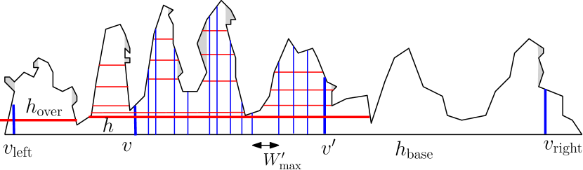
Figure 12: Top: Case (1): $v$ is not crossed by a horizontal laser. Bottom: Case (2) $v$ is crossed by a horizontal laser; $h$ is the lowest such laser. The pockets are shown in gray shading.

If $k_{v}\geq 3$, then we optimize over the choice of the leftmost vertical laser cut, $v$, within $P_{\sigma}$, considering two possibilities:

(1)

In the optimal solution, $v$ is not crossed within $P_{\sigma}$ by a horizontal laser.

In this case,

$$f(\sigma)=\min_{v}\{f(\sigma^{\prime})+H(v_{\rm left},v,h_{\rm over})\},$$

with $H(v_{left},v,h_{over})$ equal to the minimum number of horizontal lasers required in the sub-pseudo-histogram determined by $(v_{\rm left},v,h_{\rm over})$, with $\sigma^{\prime}=(h_{\rm base},k^{\prime}_{v}=k_{v}-1,v^{\prime}_{\rm left}=v,v_{\rm right},h^{\prime}_{\rm over}=NIL,W_{\rm max})$, and with the minimization being taken over $v\in V$ satisfying (i) $v$ lies strictly between (in $x$-coordinate) $v_{\rm left}$ and $v_{\rm right}$, (ii) $v$ is at distance at most $W_{\max}$ to the right of $v_{\rm left}$, and (iii) $v$ does not cross $h_{\rm over}$ (if $h_{\rm over}\neq NIL$).

(2)

In the optimal solution, $v$ is crossed by at least one horizontal laser. Let $h$ be the lowest such horizontal laser crossing $v$, let $v^{\prime}$ (possibly $v^{\prime}=v$) be the rightmost vertical laser of OPT crossing $h$, let $k^{\prime}\in\{1,2,\ldots,k_{v}\}$ be the number of vertical lasers crossing $h$ in OPT, and let $W^{\prime}_{max}$ be the maximum spacing between consecutive vertical lasers crossing $h$ in OPT.

Necessarily, the area of the piece of $P_{\sigma}$ that is left of $v$ and below $h_{\rm over}$ and below $h$ must be at most $1$. (Note that the inherited overhang constraint implies the constraint that no additional horizontal laser can cross $v_{\rm left}$ between $h_{\rm base}$ and $h_{\rm over}$.)

We get new subproblems $\sigma_{1}=(h,k^{\prime},v,v^{\prime},NIL,W^{\prime}_{\rm max})$, and $\sigma_{2}=(h_{\rm base},k_{v}-k^{\prime},v^{\prime},v_{\rm right},h,W_{\rm max})$.

In this case, the recursive optimization is given by

$$f(\sigma)=\min_{v,v^{\prime},h,k^{\prime}}\{1+f(\sigma_{1})+f(\sigma_{2})\}.$$

This concludes the description of the dynamic program.

While we have specified the algorithm for the measure of area, with slight modifications, the algorithm also applies to the measure of diameter, allowing us to solve Min-LaserDiameter in pseudo-histograms (at a much higher polynomial time bound than stated in Theorem 14.

6 Diameter Measure in Polygons with Holes and Axis-Parallel Lasers

6.1 Bi-Criteria Approximation for Diameter

In this section we give a bi-criteria approximation for the diameter version in a polygon with holes when lasers are constrained to be axis-parallel. The approach is similar to the algorithm for simple polygons and lasers of arbitrary orientations (cf. Section 4.1) in that both use grid lines, but they differ significantly to handle holes in a polygon when the lasers are axis-parallel. Particularly, in simple polygons we place lasers along grid lines, while in polygons with holes the grid lines just divide the problem into sub-problems.

Lasers in vertical strips.

Consider the infinite set of equally spaced vertical lines $\mathcal{L}_{V}=\{x=i\delta:i\in\mathbb{Z}\}$, for some $\delta>0$. The lines subdivide $P$ into a set $\mathcal{P}_{V}$ of polygons (possibly with holes), that we call strips. (Unlike Section 4.1, we do not place lasers along the lines in $\mathcal{L}_{V}$; we use the strips for a divide-and-conquer strategy.) The projection of any strip on the $x$-axis has length at most $\delta$; we say that a strip is full-width if its projection has length exactly $\delta$. Let $\mathcal{F}_{V}\subset\mathcal{P}_{V}$ denote the set of full-width strips, and let $F\in\mathcal{F}_{V}$ be a full-width strip.

The leftmost (resp., rightmost) points of $F$ lie on a line $L=\{x=i\delta\}$ (resp., $R=\{x=(i+1)\delta\}$) for some $i\in\mathbb{Z}$ (see Fig. 13). Consequently, the outer boundary of $F$ contains two simple paths between $L$ and $R$; we denote them by $T$ (top) and $B$ (bottom).

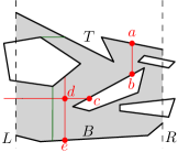
Figure 13: $F$ is shaded, the holes are white. The $L$-$R$ separating path $\gamma=abcde$ (vertices marked with red disks) alternates between holes and lasers (red) in the interior of $P$; $a_{F}(\gamma)=2$ as there are two links $ab$ and $de$ in path $\gamma$ whose extensions are fully contained in $F$. $ab$ and $cde$ are the maximal rectilinear subpaths of $\gamma$ through the free space. The minimum-link path $\gamma(F)$ (darkgreen) also alternates between holes and free space.

Since the distance between $L$ and $R$ is $\delta$, in any laser cutting of $P$ into cells of diameter at most $\delta$, there exists a $T\textrm{-}B$ path $\gamma\subset F$ along the boundaries of cells that separates $L$ and $R$. Since $\gamma$ is disjoint from the interior of the cells, it must follow lasers in the interior of $P$. We may assume, w.l.o.g., that $\gamma$ follows any laser at most once; otherwise we could shortcut $\gamma$ along the laser. Since the lasers are axis-aligned, $\gamma$ is an alternating sequence of subpaths that are either in $\partial P$ or rectilinear paths through the interior of $F$; we call any such $T\textrm{-}B$ path an alternating path.

An axis-aligned segment $s$, fully contained in $F$, is associated with $F$ if it remains fully contained in $F$ after it is maximally extended within $P$ (i.e., if both endpoints of the supporting chord of $P$ are on the boundary of $F$). For example, any vertical segment $s\subset F$ is associated with $F$ (because $T$ and $B$ belong to the boundary of $F$). Let $a_{F}(\gamma)$ be the number of associated links of $\gamma$ (i.e., the number of edges whose supporting chords are fully contained in $F$). Let $|\gamma|$ denote the total number of the (axis-aligned) edges in $\gamma$. A key observation is the following.

Lemma 18.

$|\gamma|\leq 3\,a_{F}(\gamma)$.

Proof.

Let $\pi$ be a (maximal) rectilinear subpath of $\gamma$ through the free space, i.e., a part of $\gamma$ whose endpoints lie on the boundary of $P$. If $\pi$ is a single horizontal link, then the link is associated with $F$ (because if any of its two ednpoints is outside $F$, then $\gamma$ protrudes through $L$ or $R$, not separating them). Otherwise (i.e., if $\pi$ contains vertical links), the number of the vertical links is at least 1/3 of the total number of links in $\pi$. The lemma follows by summation over all subpaths of $\gamma$. ∎

Our algorithm computes an alternating path $\gamma(F)$ with the minimum number of links and places one laser along every link of $\gamma(F)$ (the horizontal lasers may extend beyond $F$). To find $\gamma(F)$, we can build the critical graph of $F$, whose vertices are $T$, $B$, and components of $\partial P$ within the strip $F$ (including holes in the strip), and in which the weight of the edge between two vertices is the axis-parallel link distance between them. The weight of an edge between vertices $i$ and $j$ can be found by in polynomial time by standard wave propagation techniques [29, 11], i.e., by successively labeling the areas reachable with $k$ links from $i$ for increasing $k$, until $j$ is hit by the wave. After the critical graph is built, $\gamma(F)$ is found as the shortest $T\textrm{-}B$ path in the graph.

By minimality of $\gamma(F)$, the number links $|\gamma(F)|$ in it (and hence the number of lasers we place) is at most $|\gamma(F)|$. Let $k_{V}=\sum_{F\in\mathcal{F}_{V}}|\gamma(F)|$ be the total number of lasers placed in all full-width strips in $\mathcal{F}_{V}$, and let $k^{*}$ be the minimum number of axis-parallel lasers in a laser cutting of $P$ into cells of diameter at most $\delta$. An immediate consequence of Lemma 18 is the following.

Corollary 19.

$k_{V}\leq 3k^{*}$.

Proof.

As the links of $\gamma(F)$ follow lasers, at least $a_{F}(\gamma)$ lasers are fully contained in $F$. ∎

The $k_{V}$ lasers placed in full-width strips subdivide $P$ into polygonal pieces; let $Q$ be one such piece.

Lemma 20.

The length of the $x$-projection of $Q$ on the $x$-axis is at most $2\delta$.

Proof.

We prove that $Q$ intersects at most one line in $\mathcal{L}_{V}$. Suppose, to the contrary, that $Q$ intersects two consecutive lines $\ell_{1}:x=i\delta$ and $\ell_{2}=x=(i+1)\delta$. Let $\lambda$ be a shortest path in $Q$ between points in $Q\cap\ell_{1}$ and $Q\cap\ell_{2}$, respectively. By minimality, $\lambda$ lies in the strip between $\ell_{1}$ and $\ell_{2}$. Consequently, $\lambda$ is contained in some full-width strip $F\subset\mathcal{F}_{V}$. However, the path $\gamma(F)$ intersects every path in $F$ between $F\cap\ell_{1}$ and $F\cap\ell_{2}$; in particular, it intersects $\lambda$. Since we have placed a laser along every segment of $\gamma(F)$ in the interior of $P$, $\lambda$ intersects a laser, contradicting the assumption that $\lambda\subset Q$. ∎

Lasers in horizontal strips.

Similarly, we consider the set of horizontal lines $\mathcal{L}_{H}=\{y=j\delta:j\in\mathbb{Z}\}$ and apply the above process to $P$, yielding horizontal chords $C_{H}$ that subdivide the polygon into horizontal strips (polygons, possibly with holes). We again work only with full-height strips, whose boundary intersect two consecutive lines in $\mathcal{L}_{H}$. In each full-height strip, we find a minimum-interior-link rectilinear path that separates the boundary points along the two lines in $\mathcal{L}_{H}$, and place lasers along the links of the path. Let $k_{H}$ be the number of lasers over all full-height strips.

Putting everything together.

We overlay the $k_{V}$ lasers in full-width strips with the $k_{H}$ lasers in full-height strips. The resulting arrangement partitions $P$ into polygonal pieces (possibly with holes). The $x$- and $y$-projection of each piece has length at most $2\delta$ by Lemma 20; thus, each piece has diameter less than $2\delta\sqrt{2}$. By Corollary 19, the total number of lasers used in the arrangement is $k_{V}+k_{H}\leq 6k^{*}$. We obtain the following theorem.

Theorem 21.

Let $P$ be a polygon with holes of diameter ${\rm diam}(P)$ having $n$ vertices, and let $k^{*}$ be the minimum number of laser cuts that partition $P$ into pieces each of diameter at most $\delta$ for a fixed $\delta>0$. In time polynomial in $n$ and ${\rm diam}(P)/\delta$, one can compute a set of at most $6k^{*}$ lasers that subdivide $P$ into pieces each of diameter at most $2^{3/2}\delta$.

6.2 $O(1)$-Approximation to MinDiameter

Similarly to Section 4.2, we can use the bi-criteria algorithm to derive a constant-factor approximation for minimizing the maximum diameter of a cell in the arrangement of a given number $k$ of axis-parallel lasers. Our $O(1)$-approximation algorithm repeatedly decreases the $x$- and $y$- separation in the bi-criteria solution from Theorem 21 until the number of placed lasers is about to jump over 6$k$; then, the number of lasers is decreased by a factor of $6$ while increasing the diameter by a constant factor.

Specifically, let $\ell(\delta)$ denote the number of lasers used in the end of the bi-criteria algorithm with the $x$- and $y$-separation between consecutive vertical and horizontal lines being $\delta$. Our algorithm to approximate the diameter achievable with $k$ lasers is as follows:

• Initialize $\delta={\rm diam}(P)$, and let $\varepsilon>0$.

• While $\ell(\delta)\leq 6k$, set $\delta=\delta/(1+\varepsilon)$ and recompute $\ell(\delta)$.

• Let $\delta_{0}$ be such that $\ell(\delta_{0})\leq 6k$ but $\ell(\delta_{0}/(1+\varepsilon)>6k$.

• Let $\mathcal{F}_{V}$ and $\mathcal{F}_{H}$ be the full-width and full-height strips, resp., used in the bi-criteria algorithm to place the $\ell(\delta_{0})$ lasers.

• Partition $\mathcal{F}_{V}$ into 6 subsets: the set of strips whose left boundary is in a line $x=i\delta_{0}$, where $i\equiv a\mod 6$ for $a=\{0,1,2,3,4,5\}$. Let $\mathcal{F}_{V}^{\prime}\subset\mathcal{F}_{V}$ be a subset of strips that uses the minimum number of chords for their minimum-link paths.

• Similarly, partition $\mathcal{F}_{H}$ into 6 subsets of strips based on the residue class of $j\mod 6$, where the top side of the strip is in $y=j\delta_{0}$. Let $\mathcal{F}_{H}^{\prime}\subset\mathcal{F}_{H}$ be a subset that uses the minimum number of chords for their minimum-link paths.

• Return the lasers used in minimum-link paths in the strips of $\mathcal{F}_{V}^{\prime}$ and $\mathcal{F}_{H}^{\prime}$.

Theorem 22.

Let $\delta^{*}$ be the minimum diameter achievable with $k$ axis-parallel lasers. For every $\varepsilon>0$, one can compute a set of at most $k$ axis-parallel lasers that partition $P$ into pieces each of diameter at most $12\sqrt{2}(1+\varepsilon)\delta^{*}$ in time polynomial in $n$, ${\rm diam}(P)/\delta^{*}$, and $\varepsilon$.

Proof.

By Theorem 21, if $\delta^{*}$ were smaller than $\delta_{0}/(1+\varepsilon)$, then $\ell(\delta_{0}/(1+\varepsilon))$ would have been at most $6k$, which is not the case (by the choice of $\delta_{0}$), implying that $\delta^{*}\geq\delta_{0}/(1+\varepsilon)$. Our algorithm starts with at most $6k$ lasers, produced by the bi-criteria solution, that decomposes $P$ into strips that each intersect at most one line in $\mathcal{L}_{V}=\{x=i\delta_{0}:i\in\mathbb{Z}\}$ and in $\mathcal{L}_{H}=\{y=i\delta_{0}:i\in\mathbb{Z}\}$, respectively; hence their $x$- and $y$-projections have length at most $2\delta_{0}$. By removing at least $\frac{5}{6}$ of the horizontal (resp. vertical) lasers, the number of lasers drops to $k$ or below, and the cells on opposite sides of these lasers merge. However, each resulting cell intersects at most one line in $\{x=6i\delta_{0}:i\in\mathbb{Z}\}$ and at most one line in $\{y=6i\delta_{0}:i\in\mathbb{Z}\}$. Consequently, the $x$- and $y$-projection of each resulting cell is an interval of length at most $12\delta_{0}$. Hence the diameter of the final cells is at most $12\sqrt{2}\delta_{0}\leq 12\sqrt{2}(1+\varepsilon)\delta^{*}$. ∎

7 $O(\log{\rm OPT})$-approximation for Min-LaserCircle

This section considers the radius of the largest inscribed circle as the measure of cell size; in particular, in Min-LaserCircle the goal is to split the polygon $P$ (which may have holes) into pieces so that no piece contains a disk of radius 1. We give an $O(\log{\rm OPT})$-approximation algorithm for Min-LaserCircle based on reducing the problem to SetCover. The following reformulation is crucial for the approximation algorithm:

Observation 1.

A set of lasers splits $P$ into pieces of in-circle radius at most 1 iff every unit disk that lies inside $P$ is hit by a laser.

Theorem 23.

For a polygon $P$ with $n$ vertices (possibly with holes), Min-LaserCircle admits an $O(\log{\rm OPT})$-approximation in time polynomial in $n$ and ${\rm area}(P)$.

Proof.

We lay out a regular square grid of points at spacing of $\sqrt{2}$. The set of grid points within $P$ is denoted by $G$. We may assume $|G|=O({\rm area}(P))$ by a suitable (e.g., uniformly random) shift. Due to the spacing, every unit-radius disk in $P$ contains a point of $G$ (possibly on its boundary).

Consider an optimal set, $L^{*}$ of lasers that hit all unit disks that are contained within $P$. Replace each laser (chord) $c\in L^{*}$ with up to four anchored chords of the same homotopy type as $c$ with respect to the vertices of $P$ and the points $G$, obtained as follows: Shift the chord $c$ vertically down (up), while keeping its endpoints on the same pair of edges of $P$, until it becomes incident to a point in $G$ or a vertex of $P$, then rotate the chord clockwise (counterclockwise) around this point until it becomes incident to another point in $G$ or a vertex of $P$. Since every unit disk within $P$ contains a point of $G$, any unit disk within $P$ that is intersected by $c$ is also intersected by one of the shifted and rotated copies of $c$. This means that we can construct a candidate set, $C$, of $O((n+{\rm area}(P))^{2})$ chords that can serve as lasers in an approximate solution, giving up at most a factor 4 of optimal. Further, in the arrangement of the segments $C$ within $P$, any unit disk is intersected by some set of chords of $C$, thereby defining a combinatorial type for each unit disk in $P$. (Two disks are of the same type if they are intersected by the same subset of chords in $C$; one way to define the type is to associate it with a cell in the arrangement of lines drawn parallel to each chord $c\in C$ at distance 2 from $c$ on each side of $c$ – while the center of the disk is in one cell of the arrangement, the disk intersects the same chords.) Let $D$ be the polynomial-size ($O(|C|^{2})$) set of disks, one “pinned” (by two segments, from the set $C$ and the set of edges of $P$) disk per combinatorial type. By construction, any set of chords from $C$ that meets all disks of $D$ must meet all unit disks within $P$.

We thus formulate a discrete set cover instance in which the “sets” correspond to the candidate set $C$ of chords, and the “elements” being covered are the disks $D$. Since there are constant-size sets of disks that cannot be shattered, the VC dimension of the set system is constant, and an $O(\log{\rm OPT})$-approximate solution for the set cover can be found in time polynomial in the size of the instance [8]. ∎

The same algorithm works for the version in which the lasers are restricted to be axis-aligned (the only change is that the candidate set consists from the grid of axis-aligned chords through $G$ and vertices of $P$).

Acknowledgements.

We thank Peter Brass for technical discussions and for organizing an NSF-funded workshop where these problems were discussed and this collaboration began. This research was partially supported by NSF grants CCF-1725543, CSR-1763680, CCF-1716252, CCF-1617618, CCF-1439084, CNS-1938709, DMS-1800734, CRII-1755791, CCF-1910873, CNS-1618391, DMS-1737812, OAC-1939459, CCF-1540890, and CCF-2007275. The authors also acknowledge partial support from the US-Israel Binational Science Foundation (project 2016116), the DARPA Lagrange program, the Sandia National Labs and grants by the Swedish Transport Administration and the Swedish Research Council.

References

- [1] B. Armaselu and O. Daescu. Algorithms for fair partitioning of convex polygons. Theoretical Computer Science, 607:351–362, 2015.
- [2] I. Bárány, P. Blagojević, and A. Szűcs. Equipartitioning by a convex 3-fan. Advances in Mathematics, 223(2):579–593, 2010.
- [3] A. I. Barvinok. A course in convexity, volume 54 of Graduate Studies in Mathematics. AMS, Providence, RI, 2002.
- [4] A. Bezdek and K. Bezdek. A solution of Conway’s fried potato problem. Bulletin of the London Mathematical Society, 27(5):492–496, 1995.
- [5] P. V. M. Blagojević and G. M. Ziegler. Convex equipartitions via equivariant obstruction theory. Israel Journal of Mathematics, 200(1):49–77, 2014.
- [6] K. Borsuk. Drei Sätze über die -dimensionale euklidische Sphäre. Fundamenta Mathematicae, 20:177–190, 1933.
- [7] P. Bose, J. Czyzowicz, E. Kranakis, D. Krizanc, and A. Maheshwari. Polygon cutting: Revisited. In Proc. Japanese Conference on Discrete and Computational Geometry, volume 1763 of LNCS, pages 81–92. Springer, 1998.
- [8] H. Brönnimann and M. T. Goodrich. Almost optimal set covers in finite VC-dimension. Discrete and Computational Geometry, 14(4):463–479, 1995.
- [9] B. Chazelle. A theorem on polygon cutting with applications. In Proc. 23rd IEEE Symposium on Foundations of Computer Science (FOCS), pages 339–349, 1982.
- [10] H. T. Croft, K. J. Falconer, and R. K. Guy. Unsolved Problems in Geometry. Springer-Verlag, New York, 1991.
- [11] G. Das and G. Narasimhan. Geometric searching and link distance. In Proc. 2nd Workshop on Algorithms and Data Structures (WADS), volume 519 of LNCS, pages 261–272. Springer, 1991.
- [12] H. Freeman and R. Shapira. Determining the minimum-area encasing rectangle for an arbitrary closed curve. Commun. ACM, 18(7):409–413, 1975.
- [13] R. Freimer, J. S. B. Mitchell, and C. Piatko. On the complexity of shattering using arrangements. Technical report, Cornell University, 1991.
- [14] U. Gopinathan, D. J. Brady, and N. Pitsianis. Coded apertures for efficient pyroelectric motion tracking. Opt. Express, 11(18):2142–2152, 2003.
- [15] R. Guàrdia and F. Hurtado. On the equipartition of plane convex bodies and convex polygons. Journal of Geometry, 83(1):32–45, 2005.
- [16] S. C. Gustafson. Intensity correlation techniques for passive optical device detection, 1982.
- [17] R. Hassin and N. Megiddo. Approximation algorithms for hitting objects with straight lines. Discrete Applied Mathematics, 30(1):29–42, 1991.
- [18] T. He, Q. Cao, L. Luo, T. Yan, L. Gu, J. Stankovic, and T. Abdelzaher. Electronic tripwires for power-efficient surveillance and target classification. In Proc. 2nd International Conference on Embedded Networked Sensor Systems (SenSys 2004). ACM Press, 2004.
- [19] J. Hershberger and S. Suri. A pedestrian approach to ray shooting: Shoot a ray, take a walk. J. Algorithms, 18(3):403–431, 1995.
- [20] T. Jenrich and A. E. Brouwer. A 64-dimensional counterexample to Borsuk’s Conjecture. Electr. J. Comb., 21(4):P4.29, 2014.
- [21] F. John. Extremum problems with inequalities as subsidiary conditions. In Studies and Essays Presented to R. Courant on his 60th Birthday, pages 187–204. Interscience Publishers, Inc., New York, NY, 1948.
- [22] J. Kahn and G. Kalai. A counterexample to Borsuk’s conjecture. Bull. Amer. Math. Soc., 29:60–62, 1993.
- [23] R. Karasev, A. Hubard, and B. Aronov. Convex equipartitions: the spicy chicken theorem. Geometriae Dedicata, 170(1):263–279, 2014.
- [24] J. M. Keil. Polygon decomposition. In J. Sack and J. Urrutia, editors, Handbook of Computational Geometry, pages 491–518. North Holland/Elsevier, 2000.
- [25] I. Kostitsyna. Balanced partitioning of polygonal domains. PhD thesis, Stony Brook University, Stony Brook, NY, 2015.
- [26] S. Langerman and P. Morin. Covering things with things. Discrete & Computational Geometry, 33(4):717–729, 2005.
- [27] A. Maheshwari, J.-R. Sack, and H. N. Djidjev. Link distance problems. In J.-R. Sack and J. Urrutia, editors, Handbook of Computational Geometry, chapter 12, pages 519–558. North-Holland, 2000.
- [28] N. Megiddo and A. Tamir. On the complexity of locating linear facilities in the plane. Operations Research Letters, 1:194–197, 1982.
- [29] J. S. Mitchell, V. Polishchuk, and M. Sysikaski. Minimum-link paths revisited. Computational Geometry, 47(6):651–667, 2014.
- [30] R. Nandakumar and N. Ramana Rao. Fair partitions of polygons: An elementary introduction. Proceedings-Mathematical Sciences, 122(3):459–467, 2012.
- [31] J. Robertson and W. Webb. Cake-cutting algorithms: Be fair if you can. AK Peters/CRC Press, 1998.
- [32] P. Soberón. Balanced convex partitions of measures in . Mathematika, 58(1):71–76, 2012.
- [33] S. Suri. On some link distance problems in a simple polygon. IEEE Trans. Robotics and Automation, 6(1):108–113, 1990.
- [34] G. Toussaint. Applications of the rotating calipers to geometric problems in two and three dimensions. International Journal of Digital Information and Wireless Communications, 4(3):372–386, 2014.
- [35] S. Zahnd, P. Lichisteiner, and T. Delbruck. Integrated vision sensor for detecting boundary crossings. In 2003 IEEE International Symposium on Circuits and Systems (ISCAS), volume 2, 2003.
- [36] Y. Zheng, D. J. Brady, and P. K. Agarwal. Localization using boundary sensors: An analysis based on graph theory. ACM Trans. Sen. Netw., 3(4), 2007.