J-PLUS: Unveiling the brightest-end of the $\rm Ly\alpha$ luminosity function at $\rm 2.0\!<\!z\!<\!3.3$ over $\rm 1000\,deg^{2}$

We present the photometric determination of the bright-end of the Ly$\alpha\$luminosity function (at $\rm L_{Ly\alpha}\,{\gtrsim}\,10^{\,43.5}\,erg\,s^{-1}$) within four redshifts windows ($\rm\Delta\,z\,{<}\,0.16$) in the interval $\rm 2.2\!\lesssim\!z\!\lesssim\!3.3$. Our work is based on the Javalambre Photometric Local Universe Survey (J-PLUS) first data-release, which provides multiple narrow-band measurements over $\rm{\sim}1000\,deg^{2}$, with limiting magnitude $r\!\sim\!22$. The analysis of high-z Ly$\alpha\$-emitting sources over such a wide area is unprecedented, and allows to select a total of $\sim\!14,500$ hyper-bright ($\rm L_{Ly\alpha}\,{>}\,10^{43.3}\,erg\,s^{-1}$) Ly$\alpha\$-emitting candidates. We test our selection with two spectroscopic follow-up programs at the GTC telescope, which confirm as line-emitting sources $\sim\!89\%$ of the targets, with $\sim\!64\%$ being genuine $\rm z\!\sim\!2.2$ QSOs. We extend the $\rm 2.2\!\lesssim\!z\!\lesssim\!3.3$ Ly$\alpha\$luminosity function for the first time above $\rm L_{Ly\alpha}\,{\sim}\,10^{44}\,erg\,s^{-1}$ and down to densities of $\rm\sim\!10^{-8}\,Mpc^{-3}$. Our results unveil with high detail the Schechter exponential-decay of the brightest-end of the Ly$\alpha\$LF, complementing the power-law component of previous LF determinations at $\rm 43.3\!\lesssim\!Log_{10}(L_{Ly\alpha}/erg\,s^{-1})\!\lesssim\!44$. We measure $\rm\Phi^{*}=(3.33\pm 0.19)\times 10^{-6}$, $\rm Log(L^{*})=44.65\pm 0.65$ and $\rm\alpha=-1.35\pm 0.84$ as an average over the redshifts we probe. These values are significantly different than the typical Schechter parameters measured for the Ly$\alpha\$LF of high-z star-forming LAEs. This suggests that $\rm z\!>\!2$ AGN/QSOs (likely dominant in our samples) are described by a structurally different LF than $\rm z\!>\!2$ star-forming LAEs, namely with $\rm L^{*}_{QSOs}\sim 100\,L^{*}_{LAEs}$ and $\rm\Phi^{*}_{QSOs}\sim 10^{-3}\,\Phi^{*}_{LAEs}$. Finally, our method identifies very efficiently as high-z line-emitters sources without previous spectroscopic confirmation, currently classified as stars ($\sim\!2000$ objects in each redshift bin, on average). Assuming a large predominance of Ly$\alpha\$-emitting AGN/QSOs in our samples, this supports the scenario by which these are the most abundant class of $\rm z\!\gtrsim\!2$ Ly$\alpha\$emitters at $\rm L_{Ly\alpha}\,{\gtrsim}\,10^{\,43.3}\,erg\,s^{-1}$.

1 Introduction

An increasing number of recent works has been focusing on the study of high-redshift Lyman-$\alpha$ emitters (LAEs), objects showing prominent rest-frame Ly$\alpha\$emission within a spectrum (usually) devoided of other line features (e.g., Cassata et al., 2011; Nakajima et al., 2018). The spectral properties of LAEs are usually interpreted as to be coming from young ($\rm\lesssim 50\,Myr$) and low-mass ($\rm M_{*}\!<\!10^{10}\,M_{\odot}$) galaxies (e.g., Wilkins et al., 2011; Amorín et al., 2017; Hao et al., 2018; Santos et al., 2020) with small rest-frame UV half-light radii ( $\rm R\!\lesssim\!1-2\,Kpc$, as in e.g., Møller & Warren, 1998; Lai et al., 2008; Bond et al., 2012; Guaita et al., 2015; Kobayashi et al., 2016; Ribeiro et al., 2016; Bouwens et al., 2017a; Paulino-Afonso et al., 2018) which are actively star-forming ($\rm SFR\!\sim\!1-100\,M_{\odot}/yr$) and dust-poor (dust attenuation $\rm A_{V}\!<\!0.2$, see e.g., Gawiser et al., 2006, 2007; Guaita et al., 2011; Nilsson et al., 2011; Bouwens et al., 2017b; Arrabal Haro et al., 2020). When observed at high redshift, isolated and grouped LAEs would represent the progenitors of present-day galaxies and clusters, respectively, hence providing extremely valuable insights about structure formation (e.g., Matsuda et al., 2004, 2005; Venemans et al., 2005; Gawiser et al., 2007; Overzier et al., 2008; Guaita et al., 2010; Mei et al., 2015; Bouwens et al., 2017b; Khostovan et al., 2019). A basic statistical tool to study the population of high-z LAEs is the description of their number density, at a given redshift, as a function of line luminosity ($\rm L_{Ly\alpha}$), namely the Ly$\alpha\$luminosity function (LF, see e.g., Gronke et al., 2015, for a theoretical approach). Several recent works have focused on the construction of the Ly$\alpha\$LF at $\rm z\!\geq\!2$ (Gronwall et al., 2007; Ouchi et al., 2008; Blanc et al., 2011; Clément et al., 2012; Konno et al., 2016; Sobral et al., 2017, 2018b) by making use of deep observations carried over narrow sky regions (up to few squared degrees, as in e.g., Matthee et al., 2014; Cassata et al., 2015; Matthee et al., 2017b; Ono et al., 2018). Their findings describe a Ly$\alpha\$LF which follows a Schechter function (Schechter, 1976) at relatively faint line luminosity (i.e. $\rm L_{Ly\alpha}\lesssim 10^{42.5}$, see e.g., Ouchi et al., 2008; Konno et al., 2016; Sobral et al., 2016; Matthee et al., 2017a), a regime mostly occupied by low-mass star-forming galaxies (e.g., Hu et al., 1998; Kudritzki et al., 2000; Stiavelli et al., 2001; Santos et al., 2004; van Breukelen et al., 2005; Gawiser et al., 2007; Rauch et al., 2008; Guaita et al., 2011).

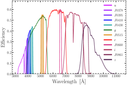
Figure 1: The measured transmission curves for the J-PLUS filter set, after accounting for sky absorption, CCD quantum efficiency and the total effect of the JAST/T80 telescope optical system. The four NB we exploit to look for bright Ly$\alpha\$emitters at $\rm z\!>\!2$ (namely, the $J$0395, $J$0410, $J$0430 and $J$0515 NBs) share their wavelength coverage with the $g$ band and are shown here as filled-area curves.

On the other hand, the bright-end of the Ly$\alpha\$LF is populated by AGN/QSOs (Calhau et al., 2020) and rare, bright and SF-bursty Ly$\alpha\$-emitting systems (e.g., Matsuda et al., 2011; Bridge et al., 2013; Cai et al., 2017b, 2018). Current constraints at high Ly$\alpha\$luminosity are somewhat poor, given the relatively small cosmological volumes probed by past works focused specifically on detecting high-z Ly$\alpha\$-emitting sources (e.g., Fujita et al., 2003; Blanc et al., 2011; Herenz et al., 2019). In particular, recent measurements show hints about a number-density excess with respect to an exponential (Schechter) decay, at $\rm L_{Ly\alpha}\gtrsim 10^{\,43}$ (e.g., Konno et al., 2016). This might be explained by means of a population of faint AGN contributing to the global LAE balance (see e.g., Matthee et al., 2017b; Sobral et al., 2018b). Further support to this picture is provided by the tomographic analysis of the high-z Ly$\alpha\$LF in the COSMOS field performed by Sobral et al. (2018b) by using a combination of optical, infrared and X-Ray data. In their work, the major contribution to the LF at $\rm L_{Ly\alpha}\gtrsim 10^{43}$ is provided by sources showing X-Ray loud counterparts, thus likely to be AGN (see also e.g., Matthee et al., 2017b; Calhau et al., 2020). Their work shows how this contribution completely vanishes at $\rm z\!\gtrsim\!3.5$, thus paralleling the peak of AGN activity usually observed at $\rm z\!\sim\!2-3$ (e.g., Hasinger et al., 2005; Miyaji et al., 2015). Finally, the constraints on the bright-end of the Ly$\alpha\$LF are prone to significant contamination by lower-redshift interlopers. For example, Sobral et al. (2017) and Stroe et al. (2017a) showed that a consistent fraction of bright LAE candidates at $\rm z\!>\!2$ are actually AGN at $\rm z\!\gtrsim\!1.5$ emitting CIV.

This work exploits the first data-release (DR1 hereafter) of the Javalambre Photometric Local Universe Survey (J-PLUS, Cenarro et al., 2019), which provides imaging of the Northern hemisphere in both narrow- and broad-bands (NB and BB, see Fig. 1 and Table 1). The DR1 covers an area of $\rm>\!1000\,deg^{2}$, which is unprecedented for NB-surveys of $\rm z\!>\!2$ luminous line-emitters. Our goal is to exploit these characteristics for obtaining large samples of photometrically-selected bright Ly$\alpha\$emitting sources, and probe the bright-end of their LF at four different redshifts (see Table 2). The combination of large survey area and multi-NB data provides the means to assess the nature of bright Ly$\alpha\$-emitting sources (Nilsson et al., 2011; Shibuya et al., 2014) and sample their distribution over a luminosity regime which is yet poorly constrained (Gronwall et al., 2007; Guaita et al., 2010; Blanc et al., 2011; Konno et al., 2016; Sobral et al., 2018b). We complement our study by presenting the results of two follow-up spectroscopic programs aimed at assessing the performance and contamination of our methodology.

This paper is organised as follows: Sect. 2 details the main features of the J-PLUS survey and the classes of sources we target. Our method for detecting NB excesses, our selection function and our sample of LAEs candidates are described in Sect. 3, along with our spectroscopic follow-up programs. Section LABEL:sec:lumifunc is focused on the computation of the four $\rm 2\!<\!z\!<\!3.3$ Ly$\alpha\$LFs. Finally, we discuss our results in Sect. LABEL:sec:scientific_results and present our conclusions in Sect. 6. Throughout this paper, magnitudes are given in the AB system (Oke, 1974; Oke & Gunn, 1983), and we assumed a flat $\Lambda$CDM cosmology described by PLANCK15 parameters (Planck Collaboration et al., 2016a, b), namely: $\rm H_{0}=67.3\,Km\,s^{-1}\,Mpc^{-1}$, $\rm\Omega_{m;0}=0.315$, $\rm\Omega_{\Lambda;0}=0.685$.

v Filter	FWHM [Å]	$\rm mag_{AB}^{min}\,(3\sigma)$	$\langle\mathit{f}_{\lambda}\rangle\ \rm(3\sigma)\ [erg\,cm^{-2}\,s^{-1}\,\text{\AA}^{-1}]$
v                             v $u$				363.91	21.17	$2.99\times 10^{-17}$
v $J$0378	152.74	21.18	$2.56\times 10^{-17}$
v $J$0395	101.39	21.06	$2.63\times 10^{-17}$
v $J$0410	201.76	21.28	$1.99\times 10^{-17}$
v $J$0430	200.80	21.30	$1.78\times 10^{-17}$
v $g$	1481.92	22.09	$7.05\times 10^{-18}$
v $J$0515	207.19	21.35	$1.18\times 10^{-17}$
v $r$	1500.20	22.02	$4.36\times 10^{-18}$
v $J$0660	146.13	21.34	$7.27\times 10^{-18}$
v $i$	1483.59	21.54	$4.47\times 10^{-18}$
v $J$0861	410.50	20.67	$7.94\times 10^{-18}$
v $z$	1055.93	20.80	$6.54\times 10^{-18}$
v

Table 1: Tabulated FWHMs and $3\sigma$ detection limits of J-PLUS filters. Additional details and information about J-PLUS DR1 can be found at: https://archive.cefca.es/catalogues/jplus-dr1. For the sake of simplicity, we generally refer to the filters $J$0378, $J$0395, $J$0410, $J$0430, $J$0515, $J$0660 and $J$0861 as J-PLUS NBs, even though some of these filters (e.g. $J$0861) could be defined as medium bands.

2 Ly$\alpha\$emitters in the J-PLUS photometric survey

J-PLUS is an ongoing wide-area photometric survey performed at the Observatorio Astrofísico de Javalambre (OAJ, Cenarro et al., 2014) in Arcos de las Salinas (Teruel, Spain). Here we summarize its technical features (detailed in Cenarro et al., 2019) and we define the class of Ly$\alpha\$-emitting sources we target.

Narrow	$\rm Ly{\alpha}$-related properties								$\ \langle\rm z\rangle$ of contaminant QSO lines
Band	$\ \langle\rm z\rangle$	$\rm z_{\,p}$	$[\rm z_{min}\ ;\ z_{max}]$	$\rm A_{eff}\ [deg^{2}]$	$\rm Vol\ [cGpc^{3}]$	$\rm F_{Ly\alpha}^{\,min}\,[erg\,cm^{-2}\,s^{-1}]$	$\rm L_{Ly\alpha}^{min}\,[erg\,s^{-1}]$	$\rm Log\,\left(L_{Ly\alpha}^{min}\right)$	SiIV	CIV	CIII]	MgII
vv                                                                                                         v $J$0395													2.24	2.25	$2.20-2.28$	897.44	0.961	$5.23\times 10^{-16}$	$2.16\times 10^{43}$	43.33	1.82	1.54	1.06	0.41
v $J$0410	2.38	2.37	$2.29-2.46$	897.46	1.917	$4.46\times 10^{-16}$	$2.21\times 10^{43}$	43.34	1.94	1.65	1.15	0.47
v $J$0430	2.54	2.53	$2.46-2.62$	897.41	1.907	$3.99\times 10^{-16}$	$2.25\times 10^{43}$	43.35	2.08	1.78	1.25	0.54
v $J$0515	3.23	3.24	$3.14-3.31$	965.99	2.044	$2.65\times 10^{-16}$	$2.68\times 10^{43}$	43.43	2.68	2.32	1.69	0.84
v

Table 2: Second to ninth columns from the left: properties of the filters related to the Ly$\alpha\$line. From left to right: median redshift in the filter bandwidth, redshift associated to the filter pivot wavelength (see Tokunaga & Vacca, 2005), redshift interval covered by the NB FWHM, effective DR1 area ad volume (see Sect. LABEL:sec:lyalum_and_volume_computation), minimum detectable line flux and luminosity (both in linear and logarithmic units, see Sect. 2.2.1). Last four columns to the right: redshift associated to strong QSOs lines (e.g., Vanden Berk et al., 2001) which can act as contaminants in our selection.

2.1 Survey description and source catalogs

J-PLUS observations are being carried out by the T80Cam instrument on the JAST/T80 83cm telescope (Marin-Franch et al., 2015). The JAST/T80 optical system provides a wide field of view ($\rm FoV\!\sim\!1.96\,deg^{2}$) while ensuring a high spatial resolution ($0.55$ arcsec/pixel, see Cenarro et al., 2019, for technical details). J-PLUS nominal depth is shallower than that of comparably-wide optical surveys, i.e. $r=22$ at signal-to-noise ratio $\rm SNR=3$ (as compared to e.g. $\rm r^{\prime}=23.1$ at $\rm SNR=5$ for SDSS, see York et al., 2000). Nevertheless, it offers NB measurements over an unprecedented sky-area, making it suitable for extensive searches of bright emission-line galaxies (ELGs). The J-PLUS filter set is composed by 12 photometric pass-band filters (see Fig. 1) which can be divided into 5 broad-bands (BBs) and 7 narrow-bands (NBs) of width $\sim\!800\!-\!2000\,\mbox{\AA}$ and $\sim\!150\!-\!500\,\mbox{\AA}$, respectively (table 1). Their measured transmission curves (i.e. accounting for optical elements, CCD quantum efficiency and sky transparency) are shown in Fig. 1.

J-PLUS images are automatically reduced in order to obtain public catalogs of sources. This work is based on the recent DR1, obtained with stable pipelines for data reduction and source-extraction, specifically calibrated and tested on J-PLUS data (as detailed in e.g., Cenarro et al., 2019; López-Sanjuan et al., 2019a). We use the standard J-PLUS dual-mode objects lists, constructed with $r$ as the band for source detection and for defining their associated sky position and photometric apertures. The latter are then used to extract sources’ photometry in the remaining filters. We note that relying on dual-mode catalogs has non-trivial implications on the completeness of our final LAEs samples, which we address in Sect. LABEL:sec:bivariate_completeness. Finally, this work is based on the DR1 auto-aperture photometry. We ensure that this choice allows to recovery the total Ly$\alpha\$line flux of point-like sources (see Sect. LABEL:sec:line_flux_retrieval) and exploit the measurement of detection completeness in each survey pointing provided in the DR1, which was tested on auto-aperture photometry (see Sect. LABEL:sec:completeness).

2.2 Detection of Ly$\alpha\$emission with J-PLUS

The design of the J-PLUS filters potentially allows to detect Ly$\alpha\$emission within seven redshift windows, one per NB, respectively centered at $\rm z\!\sim\!2.11,\,2.24,\,2.38,\,2.54,\,3.23,\,4.43$ and $6.09$. In particular, we employ the $J$0395, $J$0410, $J$0430 and $J$0515 filters (see Fig. 1) for targeting $\rm z\!\sim\!2.24,\,2.38,\,2.54$ and $3.23$, as shown in Table 2. Our selection is based on measuring NB excesses with respect to the continuum traced by BB photometry (see Sect. 3.1). Consequently, it is prone to contamination by prominent emission lines. In particular, we expect our samples to be significantly contaminated by both nebular emission due to star-formation (e.g. H$\,{}_{\beta}$, [OIII]$\!{}_{\,4959+5007}$ and [OII]$\!{}_{\,3727}$ lines) and AGN/QSOs ionizing radiation (e.g. CIV$\!{}_{\,1549}$, CIII]$\!{}_{\,1908}$, MgII$\!{}_{\,2799}$ and SiIV$\!{}_{\,1397}$ lines, see also Stroe et al., 2017a, b). The latter ones and their associated redshift intervals in J-PLUS are listed in Table 2. We note that SiIV and MgII are minor sources of contamination since: i) they are significantly fainter than Ly$\alpha\$(e.g., Telfer et al., 2002; Selsing et al., 2016), ii) J-PLUS probes relatively small cosmological volumes at $0.35\!<\rm\!z\!<\!0.85$ and iii) the number density of AGN/QSOs at $\rm z\!<\!1$ is lower than at $\rm z\!>\!2$ (e.g., Palanque-Delabrouille et al., 2016; Pâris et al., 2018). We exclude the $J$0378 NB after checking that our method does not reliably detect photometric excess in this NB (see Sect. LABEL:sec:line_flux_retrieval). We also exclude the $J$0660 and $J$0861 NBs since they provide very scarce samples of candidates ($\lesssim 100$ sources) whose contamination cannot be reliably estimated, due to the absence of cross-matches with SDSS spectroscopic data (see Sect. 3.3). We note that this is in agreement with the work of Sobral et al. (2018b), which shows no significant detection of bright ($\rm L_{Ly\alpha}\gtrsim 10^{\,43}\,erg\,s^{-1}$) Ly$\alpha\$-emitting sources at $\rm z\!\gtrsim\!3.5$, i.e. at the redshift probed by the $J$0660 and $J$0861 NBs.

2.2.1 $\rm L_{Ly\alpha}$ and $\rm EW_{Ly\alpha}$ detection limits

The minimum luminosity of an emission line measurable with a NB filter ($\rm L_{Ly\alpha}^{min}$) can be computed by knowing the relative contribution of line and continuum to the total flux in the band, and the source redshift. In other words, by knowing the line equivalent width ($\rm EW$ hereafter, see appendix A) and the wavelength position of the line-peak in the NB. Unfortunately, these are not provided by a single NB measurement without further hypothesis. To compute $\rm L_{Ly\alpha}^{min}$ for each J-PLUS NB, we first assume that faint sources are detected with higher probability at the wavelength of the transmission curve peak. Consequently their line would be redshifted to the observed $\rm\lambda_{\,obs}\!=\!\lambda_{T^{\,max}}$. The choice of $\rm EW$, on the other hand, as a higher degree of arbitrariness. Despite $\rm EW$ as low as $5\,\text{\AA}$ have been explored in the past (e.g., Sobral et al., 2017), high-z Ly$\alpha\$-emitting sources typically exhibit $\rm EW\!>\!15-20\,\text{\AA}$ (as in e.g., Gronwall et al., 2007; Guaita et al., 2010; Santos et al., 2020). We hence select $\rm EW\!=\!25\text{\AA}$ as our lower limit to estimate $\rm L_{Ly\alpha}^{min}$ (see e.g., Ouchi et al., 2008; Santos et al., 2016; Konno et al., 2018). In detail, we use the detection limits of J-PLUS bands (table 1) to compute the minimum line-flux measurable with each NB ($\rm F^{\,min}_{Ly\alpha}$, see Sect. 3.1 and appendix A for details). We then link the latter to $\rm L_{Ly\alpha}^{min}$ using our assumptions on $\rm\lambda_{\,obs}$ and $\rm EW$.

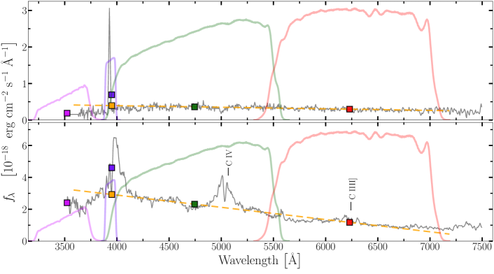
Figure 2: Representation of our NB excess detection method. Grey lines in both panels show the observed spectra of typical $\rm z\!\sim\!2$ Ly$\alpha\$-emitting sources (from the publicly available VUDS DR1 spectroscopic dataset, see e.g., Le Fèvre et al., 2015; Tasca et al., 2017). Upper panel: a SF LAE spectrum showing a single, prominent Ly$\alpha\$line (here redshifted at $\rm\lambda_{obs}\!\sim\!3900\,\mbox{\AA}$) and no other significant features. Bottom panel: a QSO spectrum with evident CIV and CIII] lines in addition to Ly$\alpha\$(at $\rm\lambda_{obs}\!\sim\!4000\,\mbox{\AA}$). We show the transmission curves and associated synthetic photometry of four J-PLUS bands as colored lines and squares. From left to right, $u$ (purple), $J$0395 NB (violet), $g$ (green) and $r$ (red). In brief: our method uses $g$ and $r$ photometry for estimating a linear continuum (yellow dashed line in the plots) which is then evaluated at the NB pivot wavelength (yellow square). Finally, the ratio between the latter and the NB measurement (violet square) is used as a proxy for the Ly$\alpha\$line flux (see Eq. 1). By using $u$ and $g$ instead of $g$ and $r$ this method would provide a poorer handle of the non-linear continuum in the region affected by the Ly$\alpha\$line profile.

The characteristics of J-PLUS filters and its observing strategy make its data sensitive to very bright Ly$\alpha\$emission ($\rm L_{Ly\alpha}\!>\!10^{\,43.3}\,erg\,s^{-1}$, see Table 2). We note that few studies have explored this range of $\rm L_{Ly\alpha}$, mostly due to the limited sky areas of their associated deep photometric surveys (see e.g., Blanc et al., 2011; Konno et al., 2016; Matthee et al., 2017b; Sobral et al., 2018b). On the contrary, J-PLUS DR1 provides multi-band imaging over $\rm\sim\!\!1000\,deg^{2}$, which is unprecedented for studies targeting high-z Ly$\alpha\$-emitting sources. The effective survey area after masking artifacts and bright stars sums up to $\rm\sim\!900\,deg^{2}$, which correspond to $\rm\gtrsim\!1\,Gpc^{3}$ (comoving) in each z window we sample (see Table 2). This allows to measure with high precision the Ly$\alpha\$luminosity function at $\rm 2.2\!\lesssim\!z\!\lesssim\!3.3$ and $\rm L_{Ly\alpha}\gtrsim 2\times 10^{\,43}\,erg\,s^{-1}$.

2.2.2 AGN/QSOs or Star-Forming galaxies

Recent compelling hints point towards identifying the majority of high-z Ly$\alpha\$-emitting sources at $\rm L_{Ly\alpha}\!>\!2\times 10^{43}\,erg\,s^{-1}$ as AGN/QSOs (see e.g., Nilsson et al., 2011; Konno et al., 2016; Matthee et al., 2017b; Sobral et al., 2018a, b; Calhau et al., 2020). The work of Sobral et al. (2018a), in particular, pointed out the co-existence of two different classes of luminous $\rm z\!\sim\!2-3$ LAEs at roughly $\rm 3\,L^{*}$, namely dust-free, highly star-forming galaxies and AGN. In addition, a significant fraction (at least $\gtrsim 20\%$) of bright LAEs selected by Matthee et al. (2017b) and Sobral et al. (2018b), respectively on the Boötes and COSMOS fields (with areas of $\rm\sim\!0.7\,deg^{2}$ and $\rm\sim\!2\,deg^{2}$) show X-Ray counterparts, which strongly points towards confirming them as AGN/QSOs. Finally, Calhau et al. (2020) shows how the fraction of AGN/QSOs within a sample of $\rm z\!>\!2$ Ly$\alpha\$-emitting candidates approaches $\sim\!100\%$ at $\rm L_{Ly\alpha}\gtrsim 10^{\,43.5}\,erg\,s^{-1}$.

We broadly expect the above findings to hold valid over the much wider area of DR1 (bigger by a factor of $\sim\!500$), hence to select a mixture of extremely Ly$\alpha\$-bright, rare star-forming galaxies (e.g., Sobral et al., 2016; Hartwig et al., 2016; Cai et al., 2017a; Shibuya et al., 2018; Cai et al., 2018; Marques-Chaves et al., 2019) and luminous AGN/QSOs, numerically dominated by the latter source class. Indeed, our work selects objects showing strong and reliable NB excess, without employing any further criterion to disentangle its nature. Figure 2 shows typical spectra of high-z SF galaxies and QSOs, pointing out their significant diversity (see e.g., Hainline et al., 2011, for a comparison with narrow-line AGN spectra). Ideally, this difference should be mirrored by bi-modalities in the photometric properties of our selected samples, assuming that i) both the Ly$\alpha\$emitting source classes are significantly present in our selection results and ii) J-PLUS filters can effectively capture their spectral difference. For generality, we conduct our analysis by considering all the sources in our selected samples as Ly$\alpha\$-emitting candidates (LAE candidates, in brief). We then look for eventual bi-modalities in their photometric properties as hints for the presence of two distinct classes of objects. Where needed, we explicitly refer to the two categories of Ly$\alpha\$-emitting sources as either QSOs or SF LAEs to clearly state this distinction.

2.2.3 Morphology of Ly$\alpha\$-emitting sources in J-PLUS data

Due to resonant scatter of Ly$\alpha\$photons by neutral hydrogen, SF LAEs can be surrounded by faint Ly$\alpha\$-emitting halos and then appear more extended at Ly$\alpha\$wavelengths than in their continuum (e.g., Møller & Warren, 1998; Fynbo et al., 2001, 2003; Nilsson et al., 2009b; Finkelstein et al., 2011; Guaita et al., 2015; Wisotzki et al., 2016; Shibuya et al., 2019, but see also Bond et al. 2010, 2012 and Feldmeier et al. 2013). As shown in Sect. 2.1, the DR1 dual-mode catalog is based on detection in $r$-band, which probes UV-continuum wavelengths in the rest-frame of $\rm z\!\gtrsim\!2.2$ sources. UV observations show typical rest-frame half-light radii of about $\rm r_{50}\!\lesssim\!2\,kpc$ for $\rm z\!\gtrsim\!2$ SF LAEs (see e.g., Venemans et al., 2005; Taniguchi et al., 2009; Bond et al., 2009, 2012; Kobayashi et al., 2016; Ribeiro et al., 2016; Paulino-Afonso et al., 2017, 2018). This translates into apparent sizes comparable to the spatial resolution of T80cam ($\rm R=0.5$”$/pixel$) and to the typical J-PLUS seeing (i.e. $s\lesssim 1^{\prime\prime}$, Cenarro et al., 2019). Since QSOs are point-like by definition, we then expect both SF LAEs and QSOs at $\rm 2.2\!\lesssim\!z\!\lesssim\!3.3$ to show compact morphology in the J-PLUS $r$ band. Section 3.3.3 details how we exploit this assumption to look for potential low-z interlopers.

Furthermore, the extended Ly$\alpha\$halos of SF LAEs are usually characterized by low surface brightness and hence observed by means of very deep NB imaging (e.g. $\rm m_{NB}\gtrsim 26-27$, see Leclercq et al., 2017; Bădescu et al., 2017; Erb et al., 2018) or IFU surveys (e.g., Bacon et al., 2015; Drake et al., 2017). This also applies to the peculiar class of high-z Ly$\alpha\$-emitting systems showing rest-frame very extended ($\rm d\gtrsim 20-30$ kpc) and bright ($\rm L_{Ly\alpha}\!>\!10^{\,43}\,erg\,s^{-1}$) Ly$\alpha\$emission, namely Ly$\alpha$-nebulae or blobs (i.e. LABs, see e.g., Matsuda et al., 2004; Bridge et al., 2013; Ao et al., 2015; Cai et al., 2017b; Cantalupo et al., 2019; Lusso et al., 2019). Despite extended Ly$\alpha\$emission being usually too faint for J-PLUS detection limits, extremely rare but sufficiently bright Ly$\alpha\$-emitting extended sources might still be observed within the very large area of J-PLUS DR1. These should be targeted by not relying on dual-mode catalogs but instead on analysing the 511 continuum-subtracted NB images of J-PLUS DR1 and applying specific source extraction criteria (as in e.g., Sobral et al., 2018b). Nevertheless, we did not focus on these tasks since they deserve a separate and detailed analysis which lies outside the goals of this work.

3 Ly$\alpha\$-emitting candidates selection

In order to select our candidates from the J-PLUS DR1, we first look for secure NB emitters (i.e. objects showing a reliable NB excess) for each of the four NBs we use. We then exploit cross-matches with external databases and the remaining J-PLUS NBs to remove low-z interlopers. Our selection rules are detailed in Sect. 3.2 and 3.3, while the following section explains how we target Ly$\alpha\$emission with J-PLUS NBs.

3.1 Detection of NB excess with a set of three filters

Our method to estimate the eventual NB excess for all DR1 sources and assess its significance is based on the works of Vilella-Rojo et al. (2015) and Logroño-García et al. (2019) which parallel well-established methodologies (see e.g., Venemans et al., 2005; Pascual et al., 2007; Gronwall et al., 2007; Guaita et al., 2010). We employ sets of three filters composed as: [NB; $g$; $r$], where NB stands for either $J$0395, $J$0410, $J$0430 or $J$0515. By using spectroscopically identified $\rm z\!>\!2$ QSOs, we checked that filter-sets defined as [NB; $u$; $g$] provide less accurate Ly$\alpha\$flux measurements than [NB; $g$; $r$]. As detailed in Vilella-Rojo et al. (2015), our method assumes that:

1. the emission line profile can be approximated by a Dirac-delta centered at a given wavelength $\rm\lambda_{EL}$,

2. the source continuum is well traced by a linear function over the wavelength range covered by the three filters.

Hypothesis 2 implies that NB measurements affected by an emission line should exhibit a photometric excess with respect to the straight line graced by $g$ and $r$ photometry (see Fig. 2). The goal of our method is to measure this excess and relate it to the line flux which is producing it.

All the NBs we use share their probed wavelength ranges with the $g$ filter, hence the eventual emission-line flux would affect also the $g$ measurement and must be removed in order to estimate the source continuum. As detailed in appendix A, we combine the NB, $g$ and $r$ fluxes (respectively $\rm f_{\lambda}^{\,NB}$, $\mathrm{f}_{\lambda}^{\,g}$ and $\mathrm{f}_{\lambda}^{\,r}$) to estimate the line-removed continuum-flux in the $g$ and NB filters (respectively $\rm f_{\lambda\,;\,cont}^{\,\mathit{g}}$ and $\rm f_{\lambda\,;\,cont}^{\,NB}$). In this way, we can estimate the eventual NB excess due only to an emission-line as:

$$\rm\Delta m^{NB}=m^{NB}_{cont}-m^{NB}=2.5\,Log\,\left(\frac{f_{\lambda}^{\,NB}}{f_{\lambda\,;\,cont}^{\,NB}}\right)\ ,$$ (1)

where the last equality follows by the definition of AB magnitudes $\rm f^{\,NB}_{\lambda}$ ($\rm m^{NB}$) is the total NB flux (magnitude) including continuum and line contributions, while $\rm f^{\,NB\,;\,cont}_{\lambda}$ ($\rm m^{NB}_{cont}$) is the continuum-only NB flux (magnitude), shown as a yellow square in Fig. 2. $\rm\Delta m^{NB}$ is an indirect probe of $\rm F_{Ly\alpha}$, i.e. the continuum-subtracted integrated line flux emitted by a given source. As fully detailed in appendix A, by introducing the coefficients

$$\rm\alpha_{x}=\frac{\int\lambda^{2}\,T_{\lambda}^{\,x}\,d\lambda}{\int T_{\lambda}^{\,x}\,\lambda\,d\lambda}\quad;\quad\quad\beta_{x}=\frac{T_{\lambda}^{\,x}(\lambda_{EL})\,\,\lambda_{EL}}{\int T_{\lambda}^{\,x}\,\lambda\,d\lambda}\ ,$$ (2)

which only depend on the transmission curve of a given filter “x” (i.e. $\rm T^{\,x}_{\lambda}$) and on $\rm\lambda_{\,EL}$ (i.e. the wavelength position of the line-peak in the NB), our methodology can directly estimate $\rm F_{Ly\alpha}$ via the quantity:

$$\mathrm{F^{\,3FM}_{Ly\alpha}}=\frac{\left(\mathrm{f}^{\,g}_{\lambda}-\mathrm{f}^{\,r}_{\lambda}\right)+\frac{\alpha_{r}\,-\ \alpha_{g}}{\alpha_{\mathrm{NB}}\,-\ \alpha_{r}}\cdot\left(\mathrm{f}_{\mathrm{NB}}-\mathrm{f}^{\,r}_{\lambda}\right)}{\beta_{g}+\frac{\alpha_{r}\,-\ \alpha_{g}}{\alpha_{\mathrm{NB}}\,-\ \alpha_{r}}\cdot\beta_{\mathrm{NB}}}\ .$$ (3)

We use $\rm\Delta m^{NB}$ for selecting reliable NB excesses (section 3.2), while $\rm F^{3FM}_{Ly\alpha}$ for computing the luminosity of our candidates (section LABEL:sec:lumifunc). In Eq. 3, the superscript 3FM (as in three-filters method) points out that our method provides a photometric estimate of $\rm F_{Ly\alpha}$. The biases affecting $\rm F^{\,3FM}_{Ly\alpha}$ are addressed in Sect. LABEL:sec:line_flux_retrieval.

Figure 2 graphically explains our method, when applied to both a SF LAE and a QSO spectrum. In general, SF LAEs show narrow Ly$\alpha\$-line profiles as opposed to QSOs, whose emission can easily cover (observed) intervals of few $\sim\!100\text{\AA}$. This implies that part of QSOs’ Ly$\alpha\$flux can lie outside the NB wavelength coverage, hence might be undetected by J-PLUS NBs. The importance of this bias on $\rm F^{\,3FM}_{Ly\alpha}$ depends on e.g. line profile details and the position of its peak in the NB. In turn, these are determined by a number of complex aspects, such as the QSOs accretion status (e.g., Calhau et al., 2020), the transfer of Ly$\alpha\$photons in the hydrogen-rich ISM and IGM (e.g., Dijkstra, 2017; Gurung-Lopez et al., 2018) or the sources’ metals and dust content (e.g., Christensen et al., 2012). These details can be extracted by high-resolution spectroscopic data but not from J-PLUS photometry. For this reason, we apply Eq. (3) to all our selected candidates and then statistically correct $\rm F^{3FM}_{Ly\alpha}$ to account for the line-flux loss, as detailed in Sect. LABEL:sec:filter_width_corr.

3.2 Selection Function

We extract our $\rm 2.2\!\lesssim z\lesssim\!3.3$ LAE candidates from a parent sample of $\rm N\!\sim\!1.1\times 10^{7}$ sources, obtained from the J-PLUS DR1 $r$-band selected, dual-mode catalog (see Sect. 2.1 and Cenarro et al., 2019). Our selection targets strong NB excesses with respect to the BB-estimated continuum and removes secure contaminants (see Sect. 3.3). Its overall performance was significantly improved thanks to the spectroscopic follow-up programs described in Sect. 3.4. The selection results are presented in Sect. LABEL:sec:LAE_samples, while the implications of using dual-mode catalogs are addressed in Sect. LABEL:sec:line_flux_retrieval and LABEL:sec:completeness.

The photometry of too-bright or too-faint objects is likely to be either saturated or severely affected by noise. Hence we apply a very broad cut on $g$, $r$ magnitudes and their associated errors ($\rm\sigma_{\mathit{g}}$ and $\rm\sigma_{\mathit{r}}$), namely:

• $14\leqslant$ $g$ $\leqslant 24\ \bigwedge\ \rm\sigma_{\mathit{g}}<1$   ;   $14\leqslant$ $r$ $\leqslant 24\ \bigwedge\ \rm\sigma_{\mathit{r}}<1$.

We check that these conditions do not significantly affect the final number of our candidates. Nevertheless, we account for eventual losses of continuum-faint sources with relatively bright Ly$\alpha\$emission (see Sect. LABEL:sec:completeness). Spurious detections eventually included in these $g$ and $r$ intervals are removed by adequate SNR cuts (see below).

We additionally require single-mode detection in each of the NB, $g$ and $r$ bands, since all are necessary for our excess-detection method. For this, we exploit the detection flags provided by the DR1 database. This condition implies that we are only sensitive to low EW at faint Ly$\alpha\$flux; we account for this in our completeness estimates (section LABEL:sec:completeness).

The normalized effective exposure time $\rm t^{\,eff}_{\,exp}$ (provided in the DR1) can be used as a proxy for the number of exposures contributing to the photometry of each source. The limit $\rm t^{\,eff}_{\,exp}>0.5$ excludes objects whose detection is affected by the dithering pattern of J-PLUS pointings, which might compromise the removal of cosmic rays or their extraction process.

Sources’ photometry can be affected by optical artifacts or bright stars. J-PLUS makes use of the MANGLE software (Swanson et al., 2008) in order to mask-out areas affected by these defects. For each of our selection, we apply the cumulative MANGLE mask associated to the three-filters [NB; $g$; $r$]. This reduces the total sky-coverage of our data to an effective area of $\rm A_{eff}\sim 900\,deg^{2}$ (see Table 2 for details).

3.2.1 Pointing-by-pointing selection

The combined action of the previous cuts produce four different lists (one per NB) of $\rm N\gtrsim 2\times 10^{6}$ sources each (see Table 4). To proceed, we take into account that J-PLUS DR1 is composed by 511 different pointings (or tiles) which exhibit e.g. varying depths, source counts and colors. Consequently, we apply the following conditions on each tile separately build a selection function as uniform as possible.

NB excess significance

In order to select line-emitters candidates, we look for outliers in the $\rm\Delta m^{NB}$ vs. $\rm m^{NB}$ distribution of each tile, after considering photometric uncertainties (as in e.g., Bunker et al., 1995; Fujita et al., 2003; Sobral et al., 2009; Bayliss et al., 2011; Matthee et al., 2017b, and Fig. 3). In particular, using Eq. 1 we compute the error:

$$\rm\sigma_{\Delta m^{NB}}(m^{NB})=\sqrt{\rm\sigma_{m^{NB}_{cont}}^{2}+\sigma_{m^{NB}}^{2}}\ ,$$ (4)

and identify reliable NB-emitters as the objects satisfying:

$$\rm\Delta m^{NB}>\Sigma\cdot\sigma_{\Delta m^{NB}}+\langle\Delta m^{NB}\rangle\ ,$$ (5)

with $\Sigma=3$. We account for pointing variations by anchoring our cut to the average color $\rm\langle\Delta m^{NB}\rangle$ of each tile, which acts as a rigid offset. Figure 3 shows the results of this procedure on a J-PLUS tile with $\rm\langle\Delta m^{NB}\rangle=-0.27$. As expected, only $\lesssim\!10-15\%$ of our parent-sample pass this cut (see Table 4).

We explicitly exclude objects with low-SNR NB measurements by imposing $\rm m_{\,NB}\!>\!m^{NB}_{cut}$, where $\rm m^{NB}_{cut}$ is the NB magnitude at which the average NB SNR of each pointing is equal to $5$. This threshold is relatively impacting on the whole DR1, since only $\sim 35\%$ of sources is able to pass it. We checked that imposing $\left\langle\rm SNR\right\rangle=3$ would lead to significantly higher contamination of our selected samples.

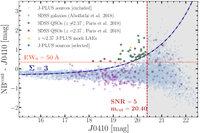
Figure 3: Example of a color-magnitude diagram obtained for the NB filter $J$0410 on a DR1 pointing (out of 511). Our photometric cuts are summarized as follows: the blue dashed-dotted line shows the $\rm\Delta m^{NB}$-significance threshold, while the vertical red line marks the NB SNR limit. We exclude sources below the blue dashed-dotted line and inside the grey shaded area. The orange horizontal dotted line shows $\rm\Delta m^{NB}$ associated to $\rm EW=50\text{\AA}$ (see Eq. 7). Grey-blue dots mark all the J-PLUS detections in the pointing, while red and purple crosses show $\rm z\!\sim\!2.4$ QSOs and low-z galaxies from SDSS DR14. Yellow triangles show J-PLUS mock data of $\rm z\!\sim\!2.4$ SF LAEs (Izquierdo-Villalba et al., 2019). Finally, our Ly$\alpha\$-emitting candidates are shown as green dots.

Clean BB photometry is a key requirement to estimate the sources NB excess. We exclude objects with $g$ $\rm\!>\!g_{cut}$ and $r$ $\rm\!>\!r_{cut}$, where $\rm g_{cut}$ and $\rm r_{cut}$ are defined as the magnitudes at which $\rm\langle SNR\rangle=5$ in each BB and pointing. Despite its effect on the parent samples being small (see Table 4), this cut might exclude genuine continuum-faint candidates with bright Ly$\alpha\$. We account for this as described in Sect. LABEL:sec:completeness.

In principle, Ly$\alpha\$can be distinguished from e.g. CIV and CIII] of AGN/QSOs spectra (e.g., Stroe et al., 2017a, b) or nebular H$\,{}_{\beta}$, [OIII]$\!{}_{\,4959+5007}$ and [OII]$\!{}_{\,3727}$ by exploiting its generally higher intrinsic strength and EW (e.g., Vanden Berk et al., 2001; Hainline et al., 2011; Selsing et al., 2016; Nakajima et al., 2018). Therefore, we impose a NB-color cut defined by assuming a minimum rest-frame EW for our candidates (as in, e.g. Fujita et al., 2003; Gawiser et al., 2006; Gronwall et al., 2007; Hayes et al., 2010; Adams et al., 2011; Clément et al., 2012; Santos et al., 2016). Observed- and rest-frame EWs (respectively $\rm EW_{obs}$ and $\rm EW_{0}$) are related via:

$$\rm EW_{obs}=EW_{0}\ (1+z)\ .$$ (6)

We set $\rm EW_{0}^{\,min}=50\,\text{\AA}$ and obtain the corresponding $\rm EW_{obs}^{\,min}$ from Eq. (6). We then link $\rm EW_{obs}$ and $\rm\Delta m^{NB}$ (defined in Eq. 1) with the analytic expression:

$$\rm\Delta m^{NB}_{min}=2.5\,Log\,\left(1+\beta_{NB}\cdot EW_{obs}^{min}\right)+\langle m^{NB}\rangle\ ,$$ (7)

(see Guaita et al., 2010, and appendix A), where $\rm\beta_{NB}$ is defined in Eq. 2 and $\rm\langle m^{NB}\rangle$ is the average color in the tile. By requiring $\rm\Delta m^{NB}\!>\!\Delta m^{NB}_{min}$ (orange horizontal dotted line in Fig. 3) we exclude $\gtrsim 96\%$ of our DR1 parent sample, since most sources do not show line-emission. We note that the choice of $\rm EW_{0}^{\,min}$ has a certain degree of arbitrariness indeed past works have explored a wide range of limiting values (see e.g., Gronwall et al., 2007; Ouchi et al., 2008; Bond et al., 2009; Nilsson et al., 2009b; Guaita et al., 2010; Konno et al., 2016; Matthee et al., 2016; Bădescu et al., 2017; Sobral et al., 2017). We fix $\rm EW_{0}=50\text{\AA}$ after checking our EW estimates on publicly-available spectroscopic catalogs of $\rm z\!\gtrsim\!2$ SF LAEs and QSOs (namely DR14, VUDS and VVDS Cassata et al., 2011; Le Fèvre et al., 2015; Pâris et al., 2018) and on the confirmed $\rm z\!\sim\!2$ QSOs in our follow-up data (see Table 8 in Sect. 3.4). In particular, $50\text{\AA}$ provides a good compromise between the retrieval of $\rm z\!\gtrsim\!2$ sources and the exclusion of $\rm z\!<\!2$ interlopers. We note that this relatively high $\rm EW_{0}^{\,min}$ is still close to the lower limits of EW distributions usually measured for high-z Ly$\alpha\$-emitting sources (e.g., Nilsson et al., 2009a; Bond et al., 2012; Amorín et al., 2017; Hashimoto et al., 2017; Santos et al., 2020). Besides, low EWs can be accessed with very-narrow bands ($\rm FWHM\!\lesssim\!50\text{\AA}$) and deep observations ($r\!>\!22$, e.g., Sobral et al., 2017), which both act as limiting factors in our case. Finally, we stress that this condition is not directly applied on $\rm EW_{0}$, hence it does not pose a strict limit on the measured $\rm EW$ of our candidates (see Ouchi et al., 2008, for a similar discussion).

These cuts select respectively 12251, 19905, 24813 and 15213 objects for $J$0395, $J$0410, $J$0430 and $J$0515 NBs (i.e. $<\!1\%$ of the parent catalog, see Table 4). These samples are still likely to be contaminated by interlopers, such as lower-z QSOs, ELGs and faint blue stars, which are usually targeted with BB-based color cuts (e.g., Ross et al., 2012; Ivezić et al., 2014; Peters et al., 2015; Richards et al., 2015). We checked that, in our case, these methods significantly affect also the number of selected $\rm z\!\gtrsim\!2$ QSOs from SDSS DR14. We hence decided to drop any color cut because of its non-trivial effect on our selection.

v Filters	DR1 parent sample	$\rm\Delta m^{\,NB}$ significance	NB SNR	BB SNR	$\rm EW_{obs}^{\,min}$	First selection
v                                                         v $J$0395							2,036,657	348,613 (17.1%)	1,324,373 (65.0%)	2,017,720 (99.1%)	57,800 (2.8%)	12,251 (0.6%)
v $J$0410	2,730,135	232,753 (8.5%)	1,846,144 (67.6%)	2,679,515 (98.2%)	150,321 (5.5%)	19,905 (0.7%)
v $J$0430	3,015,684	235,685 (7.8%)	2,024,629 (67.2%)	2,930,026 (97.2%)	173,388 (5.8%)	24,813 (0.8%)
v $J$0515	4,520,911	244,550 (5.4%)	2,956,154 (65.4%)	3,797,178 (84.0%)	143,662 (3.2%)	15,213 (0.3%)
v

Table 3: Number counts of sources passing each cut of our selection, for the four J-PLUS NBs we use. Here we report the effects of each cut separately to highlight its effect, hence the fractions reported in the Table do not add to 100%. The most impacting cuts are those on $\rm EW_{obs}^{\,min}$ cut and on NB excess significance. The number of sources passing all these conditions, for each NB, produce our final samples of LAE candidates and is shown in the last column to the right. These partial samples are likely to be highly contaminated by interlopers showing reliable NB excess. Table 3.3.2 shows a summary of the samples contamination and the final number of selected sources.

3.3 Removal of residual contaminants

Despite efficiently identifying NB-emitters, the conditions in Sect. 3.2 might also select line-emitting interlopers (see Sect. 2.2). Previous works based on similar methods have usually explored limited sky regions already surveyed by deep multi-wavelength data, which supported the identification of contaminants (e.g. COSMOS, UDS, SXDS, SA22 and Boötes fields, see Warren et al., 2007; Scoville et al., 2007; Furusawa et al., 2008; Geach et al., 2008; Kim et al., 2011; Bian et al., 2012; Stroe & Sobral, 2015). Unfortunately, few previous surveys uniformly cover the very wide area of J-PLUS DR1, hence limiting our ability to identify contaminants.

3.3.1 Cross-matches with public external databases

Interlopers with a secure identification (either spectroscopic, astrometric or photometric) can be removed via cross-matches with public catalogs. We employ a radius of $\rm r_{max}^{\,match}=3.5$” after checking that this provides a high matching completeness while keeping low the number of multiple matches, for all the matched databases. More in detail, we recover the 80% (95%) of all QSOs from SDSS DR14 (within the DR1 footprint) respectively at $r\!\sim\!21.25$ ($r\!\sim\!20.80$) and $\rm Log\,(L_{Ly\alpha})\!\sim\!44.25$ ($\sim\!44.70$).

We exploit the lists of spectroscopically-identified galaxies (Bundy et al., 2015; Hutchinson et al., 2016), stars (Majewski et al., 2017) and QSOs (Pâris et al., 2018) provided by the recent SDSS-IV DR14 (DR14 hereafter, Blanton et al., 2017; Abolfathi et al., 2018). Given the wide overlap with J-PLUS DR1 and the higher depth of DR14 (Cenarro et al., 2019), this cross-match ensures the removal of secure contaminants from our selection. As discussed in Sect. 2.2, QSOs can act as both interlopers and genuine candidates depending on their z, hence we need to rely on a list of securely identified QSOs. The Pâris et al. (2018) catalog includes $\rm N\gtrsim 5.3\times 10^{5}$ sources observed by BOSS and eBOSS surveys (Dawson et al., 2013, 2016) and confirmed as QSOs by careful inspection. We keep genuine Ly$\alpha\$-emitting sources at the z sampled by each NB, while the rest are identified as contaminants and removed. The cross-match with DR14 shows a generally low contamination (table 3.3.2), with low-z galaxies accounting respectively for 5.1%, 4.3%, 5.3% and 3.1% of our $J$0395, $J$0410, $J$0430 and $J$0515 NB samples. On the other hand, the $\rm z\!\lesssim\!2$ QSOs fraction drops from 11.1% to 0.3%, paralleling the drop of DR14 $\rm z\!\gtrsim\!2.2$ QSOs. Finally, SDSS stars account for $\lesssim\!2\%$ of our samples. These fractions are likely to be underestimated, given the different depth of the two surveys and eventual mis-matches between DR14 and DR1 catalogs. Nevertheless, being measured on spectroscopically confirmed sources, these are secure contamination estimates.

Our spectroscopic follow-up program 2018A (see Sect. 3.4) showed a non-negligible contamination from stars in our samples. To limit this issue, we built a specific criterion for excluding stars, based on the very accurate measurements offered by Gaia DR2 data (Gaia Collaboration et al., 2018). Since the latter do not include source classification, we define secure stars by using the significance of their proper-motion assessments. More in detail, we exclude the J-PLUS sources with a counterpart in Gaia DR2, showing significant measurements ($\sigma\!>\!3$) in each proper motion component, i.e.:

$$\rm\sigma_{pm}=\sqrt{\rm\sigma_{pmra}^{2}+\sigma_{pmdec}^{2}+\sigma_{\mu}^{2}}>\sqrt{27}\sim 5.2\ ,$$ (8)

where $\rm\sigma_{pmra}$, $\rm\sigma_{pmdec}$ and $\rm\sigma_{\mu}$ are respectively the errors on proper motion (ra and dec) and parallax. With this cut, we explicitly remove objects showing significant apparent motion from our list of LAE candidates. The good performance of this criterion was confirmed by the results of our second follow-up program, whose targets were selected from the results of our updated pipeline (see Sect. 3.4 for details). The contamination from Gaia DR2 is presented in Table 3.3.2.

Ly$\alpha\$-emitting sources at $\rm z\!>\!2$ are generally expected to appear faint at (observed) UV wavelengths due to the dimming action of the Ly$\alpha\$-break and Lyman-break (e.g., Steidel & Hamilton, 1992; Steidel et al., 1996, 1999; Shapley et al., 2003). On the contrary, $\rm z\!<\!2$ AGN/QSOs, blue stars and low-z star-forming galaxies can show significant UV emission. We exploit this property for removing $\rm z\!<\!2$ interlopers by cross-matching our catalogues with GALEX all-sky UV observations (Gil de Paz et al., 2009). In particular, we remove sources with a $\rm SNR\!>\!3$ detection in either of the two FUV and NUV GALEX bands (see e.g., Ciardullo et al., 2012). Table 3.3.2 shows the fraction of interlopers identified with this cross-match in each NB. In order to check our assumption according to which only $\rm z\!<\!2$ sources are expected to be significantly observed in UV, we additionally matched the J-PLUS sources with counterparts in GALEX to the spectroscopic sample of DR14. This analysis confirmed that $>\!99.5\%$ of sources with UV-bright GALEX detection show a spectroscopic $\rm z\!<\!2$, hence act as contaminant in our selection.

The third release of the Large Quasar Astrometric Catalog (Souchay et al., 2015a, b) is a complete archive of spectroscopically identified QSOs. By combining data from available catalogs, it provides the largest complement to the DR14 list (Pâris et al., 2018). We exclude sources included in LQAC-3 with spectroscopic z lying outside the range probed by each NB. As expected, this step identifies only few additional interlopers (see Table 3.3.2).

3.3.2 Multiple NB excesses

We target additional interlopers by exploiting the whole set of J-PLUS NBs. In particular, we look for LAE candidates showing significant excesses (with respect to adjacent BBs) in the six NBs not used for their selection. Indeed, we expect SF LAEs to not show any additional NB feature (e.g., Shapley et al., 2003; Nakajima et al., 2018), while QSOs at the targeted z can exhibit only particular combinations of NB excesses.

Figure 4: Examples of multiple NB excess in J-PLUS photo-spectra. Empty and filled squares respectively mark NB and BB photometry, while the dashed yellow line shows the linear continuum we estimate through $g$ and $r$ BBs (in green and red, respectively). This comparison shows that both a $\rm z\!\sim\!0.05$ galaxy (upper panel) and a $\rm z\!\sim\!2.25$ QSO (lower panel) exhibit significant excesses in $J$0395 and $J$0515 NBs (respectively second and fifth empty squares from the left). The $J$0515 excess is produced respectively by H$\,{}_{\beta}$ at $\rm z\!\sim\!0.05$ and CIV line at $\rm z\!\sim\!2.25$, but its nature is hardly distinguishable by J-PLUS photometry.

Consequently, we remove the sources showing multiple excesses not compatible with $\rm z\!>\!2$ spectral features (e.g., Matthee et al., 2017b). On the other hand, sources showing multiple excesses compatible with $\rm z\!>\!2$ sources can hardly be separated into different classes by J-PLUS data. As an example, Fig. 4 shows the photo-spectra of a $\rm z\!\sim\!0.05$ galaxy (upper panel) and a $\rm z\!\sim\!2.25$ QSO (bottom panel) from the DR14 spectroscopic samples. Both sources show simultaneous excesses in $J$0395 and $J$0515 filters (respectively purple and yellow empty squares) with respect to the linear continuum traced by $g$ and $r$ BBs (yellow dashed line). On top of this, both photo-spectra exhibit comparable BB colors and might hence be confused by our selection. Since we are not able to directly measure this source of contamination, we estimate a statistical correction as explained in Sect. LABEL:sec:purity_of_samples.

v Filters	First selection	SDSS spectra	GALEX	Gaia DR2 stars	LQAC QSOs	Multiple NB	Extended	Final [N; $\rm deg^{-2}$]
v $J$0395	12,251	2,192 (17.9%)	2,003 (16.4%)	857 (7.0%)	87 (0.7%)	1,312 (10.7%)	6,307 (51.5%)	2,547 ; 2.8
v $J$0410	19,905	1,983 (9.9%)	2,003 (10.1%)	2,738 (13.8%)	56 (0.3%)	16,48 (8.3%)	9,557 (48.0%)	5,556 ; 6.2
v $J$0430	24,813	2,083 (8.4%)	2,597 (10.5%)	2,441 (9.8%)	40 (0.2%)	3,313 (13.4%)	15,468 (62.3%)	4,994 ; 5.6
v $J$0515	15,213	523 (3.4%)	1,249 (8.2%)	531 (3.5%)	7 (0.05%)	1,282 (8.4%)	12,992 (85.4%)	1,467 ; 1.5
v

Table 4: Number counts (and fractions) of secure interlopers among the sources passing our photometric selection, for each J-PLUS NB we use (see discussion in Sect. 3.3). We note that the extended fraction of our samples is particularly high for the $J$0515 NBs, suggesting that this filter is affected by high level of contamination from extended low-z interlopers. Indeed, this is the only NB among the four which is susceptible to contamination from the strong [OIII]$\,{}_{4959+5007}$ doublet and H$\,{}_{\beta}$ line, in addition to [NeIII] and [OII]. Sources with at least one identification as secure interloper are excluded; the final number counts of Ly$\alpha\$-emitting candidates are shown in the last column to the right. The average sky density of these objects shows significant variation among the four lists, with an average of $\rm\sim 4\,deg^{-2}$ sources, per filter. The complete catalogs of genuine candidates (i.e. after excluding securely identified interlopers) can be found at: https://www.j-plus.es/ancillarydata/dr1_lya_emitting_candidates

3.3.3 Morphological cut

We expect our $\rm z\!\gtrsim\!2.2$ candidates to appear compact in J-PLUS data (see Sect. 2.2.3), hence the candidates showing extended morphology are likely to be low-z interlopers. The DR1 catalog provides a morphological parameter $\mathcal{C}$ which allows to discriminate between compact ( $\mathcal{C}\!\sim\!1$) and extended objects ($\mathcal{C}\!\sim\!0$, see López-Sanjuan et al., 2019b, for details). By cross-matching the whole DR1 sample to SDSS spectroscopic catalogs of galaxies and QSOs, we checked that more than $\gtrsim 90\%$ of galaxies in SDSS ($\rm z\!\lesssim\!1$, see Hutchinson et al., 2016) and only $\lesssim 5\%$ of DR14 QSOs (at any z) are found at $\rm\mathcal{C}\leqslant 0.1$. We then remove objects with $\rm\mathcal{C}\leqslant 0.1$ from our selection. Table 3.3.2 (previous-to-last column to the right) shows the abundance of extended sources in each of the four lists.

3.4 Spectroscopic follow-up at the GTC telescope

This section presents two spectroscopic follow-up programs executed at the Gran Telescopio Canarias (GTC) telescope in the semesters 2018A and 2019A. The spectroscopic confirmation of a sub-sample of our candidates allowed to assess the performance of our selection, to refine our methodology and to estimate its residual contamination. Overall, these programs confirmed 45 sources selected among our $J$0395 NB-emitters.

3.4.1 Programs description

To ensure uniform observations and comparable results, we performed the same target selection and required identical observing conditions for both programs (namely GTC2018A and GTC2019A). In particular, we randomly selected a sample of 24 (21) Ly$\alpha\$-bright candidates ($\rm L_{Ly\alpha}\!>\!10^{\,43.5}\,erg\,s^{-1}$) for program GTC2018A (GTC2019A), spanning the entire luminosity range covered by our candidates. We stress that targets for GTC2019A were selected after refining our selection with the help of GTC2018A results. We requested to use the OSIRIS spectrograph and the R500B grism, in order to exploit its good spectral resolution ($\rm R\!\sim\!500$, which translates to $\rm\Delta\lambda\,pixel^{-1}\!\sim\!3.65\text{\AA}$ for the 0.8” slit width we requested). The exposure times for our targets were computed by assuming the observing conditions summarized in the header of Table 8 (appendix B). These were calibrated to achieve $\rm SNR\!\geqslant\!3$ (in each $\lambda$ bin) over the whole OSIRIS spectral range, in order to identify eventual emission lines and measure their integrated flux.

We limited our programs length to $<\!20$ hours, to ensure their completion. Due to the high observing times required by our targets, we followed-up only candidates selected by $J$0395 NB. The target selection balanced the total observing time and the uniform sampling of our candidates $\rm L_{Ly\alpha}$ distribution. Finally, we excluded objects with previous spectroscopic identifications (at any z). Our proposals were respectively awarded with 11.56 and 18.95 hours of observations and were both fully executed.

3.4.2 Spectroscopic results

The results of both programs are shown in Table 8. Overall, we identified 29/45 targets ($64.4\%$) as genuine $\rm z\!\sim\!2.2$ Ly$\alpha\$-emitting sources, 8/45 ($17.7\%$) as $\rm z\!\sim\!1.5$ QSOs emitting CIV at $\rm\lambda_{obs}\sim 4000\,\texttt{\AA}$, 1 ($2.2\%$) $\rm Ly\beta$-emitting QSO at $\rm z\!\sim\!2.76$, 5 ($11.3\%$) blue stars and 2 ($4.4\%$) low-z galaxies selected because of their narrow emission lines. As an example, Fig. 5 shows a spectra for each different source class together with its associated J-PLUS photometry.

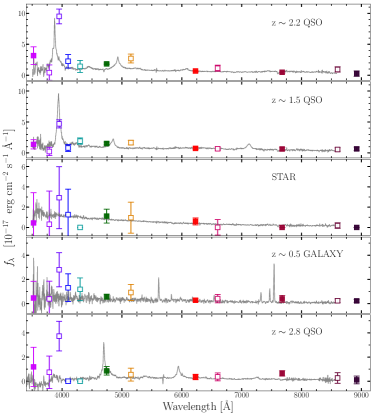
Figure 5: Summary of our spectroscopic results, showing one spectrum (grey line in each panel) for each source classes identified in our target lists. From top to bottom: $\rm z\!\sim\!2.2$ QSO, $\rm z\!\sim\!1.5$ QSO, star, $\rm z\!\sim\!0.5$ galaxy and $\rm Ly\beta\!\!$-emitting QSO. The corresponding J-PLUS photometry is shown as coloured squares. The star and galaxy targets show low-significance excesses in $J$0395 NB (third square from the left). Indeed, these interlopers were selected as targets by the first version of our methodology, i.e. before applying the improvements due to CTG2018A results and the re-calibration of J-PLUS data (López-Sanjuan et al., 2019a).

Both $\rm z\!\sim\!2.2$ and $\rm z\!\sim\!1.5$ QSOs show prominent line emission at $\rm\lambda_{obs}\sim 3950$ and are consequently selected as genuine $J$0395 NB-emitters. The same applies to the $\rm z\!\sim\!2.8$ QSO emitting $\rm Ly\beta$ at $\rm\lambda_{obs}\!\sim\!3950$. On the contrary, the remaining sources do not show significant spectral features, indeed their selection is due to strong blue colors combined to a barely-significant NB-excess (see e.g. third panel from above). In particular, the star and galaxy interlopers (i.e. third and fourth panels from the top) were picked as targets before we refined our selection rules and the J-PLUS DR1 was re-calibrated (López-Sanjuan et al., 2019a). With the current J-PLUS photometry and our updated selection these objects are not re-selected (right column of Table LABEL:tab:GTCresults2018A). Given the absence of emission lines at $\rm\lambda_{obs}\!\!\sim\!\!3900\text{\AA}$ for these objects, their low-significance NB-excess is likely due to imperfections in their photometry. In the case of the $\rm z\!\!\sim\!\!0.5$ galaxy (fourth panel from the top in Fig. 5), we additionally observe a discrepancy between the spectrum and J-PLUS data. A number of possible explanation can account for this, such as errors in the spectrum extraction and calibration, too-low spectroscopic SNR at $\rm\lambda_{obs}\lesssim 4500\,\text{\AA}$ or artifacts biasing only the $J$0395 photometry. On the contrary, the excess of the $\rm z\!\sim\!2.8$ QSO (bottom panel in Fig. 5) is due to the $\rm Ly\beta$ line redshifted at $\rm\lambda_{obs}\sim 3950$ in the observed spectrum, although in tension with J-PLUS photometry. In this case, QSO variability might play a role (e.g., Hook et al., 1994; Kozłowski, 2016) as well as photometric imperfections.

Overall, $40/45$ targets ($88.9\%$) are genuine line emitters, hence confirming the efficiency of our selection. Moreover, the stars contamination is reduced from $\sim\!17\%$ to $\lesssim\!5\%$ between the two programs (see Tables LABEL:tab:GTCresults2018A and LABEL:tab:GTCresults2019A). Indeed, guided by the GTC2018A results, we i) excluded sources with significant apparent motion according to Gaia DR2 and ii) selected $\rm EW_{0}=50\text{\AA}$ as our limiting value for defining the $\rm\Delta m^{NB}$ cut (see Sect. 3.2).

Figure 12: Ly$\alpha\$luminosity functions for each of the NB filter we used in our study (colored squares). The grey shaded areas show the Ly$\alpha\$luminosity limit (vertical limit) and the limiting number density measurable by J-PLUS (horizontal limit). The wide area explored by the narrow-bands of J-PLUS survey allow to remarkably extend the range of luminosity sampled by previous studies (coloured circles, triangles hexagons and diamonds in each plot) and to explore previously-unconstrained $\rm L_{Ly\alpha}$ intervals. Dashed lines marks the best-fit determinations by Sobral et al. (2018b), split respectively into a Schecther (light green) and a power-law contribution (dark green). Our results provide tight constraints at $\rm 44.5\lesssim Log\,(L_{Ly\alpha}/erg\,s^{-1})\lesssim 45.5$, a regime currently unexplored by previous Ly$\alpha\$LFs determinations. Our errors are dominated by the completeness correction at low luminosity, while poor statistics due to low number counts (i.e. poissonian errors) dominate the bright tail of our distributions.

We report the best fits from Sobral et al. (2018b) at each redshift since these highlight both the Schechter and power-law components of the LFs (respectively, light-green and dark-green dashed lines in Fig. 1). These are obtained from a mixed Schechter/power-law model adapted to $\rm Log(L_{Ly\alpha}/\,erg\,s^{-1})\!\lesssim\!44.5$ data, showing a transition between the two regimes at $\rm Log(L_{Ly\alpha}/\,erg\,s^{-1})\!\sim\!43.5$. Despite the small overlap of luminosity regimes, our $\rm z\!\sim\!2.25$ LF shows a remarkably good agreement with the power-law of Sobral et al. (2018b), as shown in the upper-left panel of Fig. 1. Interestingly, this component well accounts for the population of X-ray bright objects in their samples, suggesting that these sources might belong to a separate class described by a different luminosity distribution than SF LAEs at $\rm Log(L_{Ly\alpha}/\,erg\,s^{-1})\!\lesssim\!43.3$. On the contrary, a significant discrepancy between our data and the power-law components is evident at higher z. We ascribe this to the wider separation between the $\rm L_{Ly\alpha}$ ranges probed by our data and those on which the fits of Sobral et al. (2018b) are obtained at these z.

We note that our $\rm z\!\sim\!2.25$ data nicely complement also the bright-end determination of Konno et al. (2016) (orange dots in the upper-left panel of Fig. 1). This work clearly showed an excess with respect to the exponential decay of a Schechter function at $\rm Log(L_{Ly\alpha}/\,erg\,s^{-1})\!\gtrsim\!43$. Their explanation relied on the contribution of a population of Ly$\alpha\$-emitting AGN/QSOs, as in e.g. Matthee et al. (2017b) and Sobral et al. (2018b). By joining these hints to the results of our spectroscopic follow-up and our sample analysis (Sect. 3.4 and LABEL:sec:LAE_samples), our work further supports the picture according to which Ly$\alpha\$-emitting AGN/QSOs are responsible for the bright-end excess observed on the $\rm 2\!\lesssim\!z\!\lesssim\!3$ Ly$\alpha\$luminosity function at $\rm 43.3\!\lesssim\!Log(L_{Ly\alpha}/\,erg\,s^{-1})\!\lesssim\!44.5$.

5.2.1 Comparison with SDSS DR14 QSOs

Figure 1 additionally shows the Ly$\alpha\$LF of all the DR14 QSOs in the J-PLUS footprint (from Pâris et al., 2018), with spectroscopic redshift in the intervals sampled by each NB (red pentagons). We obtain this determination by performing synthetic photometry of SDSS QSOs with J-PLUS filters and applying the same flux corrections as those computed for our data (see Sect. LABEL:sec:line_flux_retrieval). For simplicity, we only associate poissonian errors to the SDSS LF.

Despite the comparison being only qualitative, the agreement between the SDSS QSOs distribution and our data is good, especially at low z. Interestingly, the fraction of our genuine candidates showing SDSS QSOs counterparts at the redshift probed by each NB is $\lesssim 30\%$, in each NB. Assuming that the Pâris et al. (2018) catalog represents a $\sim\!100\%$ complete sample of QSOS and considering the low fraction of SDSS QSOs in our data, the agreement between the two LFs could be explained in terms of a significant residual contamination of our samples ($\sim\!70\%$). Nevertheless, this is in contrast with both our purity estimates and our spectroscopic follow-up (Sect. LABEL:sec:purity_of_samples and 3.4.2). A more interesting explanation is that our NB-based selection might actually be sensitive to high-z QSOs which lack spectroscopic determination in SDSS (due e.g. to their BB colors, see Ross et al., 2012; Richards et al., 2015), as those confirmed by our follow-up programs. Indeed, their previous classification based on SDSS photometry and morphology would identify most of them just as compact objects (namely stars, see Table 8). We suggest that this mis-classification might originate from the SDSS target selection, based on BB-colors, which might miss the presence of emission lines. On the contrary, our selection targets photometric excesses with respect to a continuum estimate, hence it can efficiently select high-z line emitters.

Figure 13: Joint fit of our Ly$\alpha\$luminosity functions and literature data with a double-Schechter model (grey solid lines in each panel). This is obtained by joining the best Schechter fit from Sobral et al. (2018b) at each redshift (green dashed lines in each panel) and a second Schechter function (coloured dashed-dotted lines). We jointly fit this double-Schechter model to both our data and the literature ones leaving free the parameters of the second Schechter, in order to constrain its faint-end slope $\alpha$ at each redshift.

5.3 $\rm Ly\alpha$ LF parameters

5.3.1 The faint-end slope: power-law or double-Schechter?

As suggested by e.g. Konno et al. (2016); Matthee et al. (2017b); Sobral et al. (2018b, a) and Calhau et al. (2020), the population of bright Ly$\alpha\$-emitting sources at $\rm Log(L_{Ly\alpha}/erg\,s^{-1})\!>\!43$ is likely to be composed by a mixture of SF LAEs and AGN/QSOs. In particular, Matthee et al. (2017b) and Sobral et al. (2018b) suggest that the two source classes might be described by substantially different distributions in terms of typical number density and Ly$\alpha\$luminosity. Interestingly, the power-law component of their studies can be explained as the faint-end of a Schechter function (Schechter, 1976, see also Eq. 34) describing the QSOs luminosity distribution. Our data can effectively support this hypothesis by providing the bright-end complement to the AGN/QSOs Schechter distribution. At the same time, our analysis limited by the J-PLUS depth which prevents us to constrain its the faind-end slope at $\rm Log(L_{Ly\alpha}/erg\,s^{-1})\!\lesssim\!44$. This might significantly influence the determination of our Schechter paramters given their mutual correlation. Instead of fixing the faint-end slope to a fiducial value (as in e.g., Gunawardhana et al., 2015; Sobral et al., 2018b), we compute it by jointly exploiting our data and previous Ly$\alpha\$LF determinations, over the whole interval $\rm 41.5\!\lesssim\!Log(L_{Ly\alpha}/erg\,s^{-1})\!\lesssim\!44$. More in detail, we make use of the Schechter component from Sobral et al. (2018b) at each redshift to describe the Ly$\alpha\$LF at $\rm Log(L_{Ly\alpha}/erg\,s^{-1})\!\lesssim\!43.3$, and combine it to a second Schechter function to account for $\rm Log(L_{Ly\alpha}/erg\,s^{-1})\!\gtrsim\!44.$. We then vary the faint-end slope of the latter and, for each $\alpha$, we jointly fit the complete double-Schechter model to both our data and all the literature determinations (see Fig. 1). Finally, for each NB we obtain $\alpha$ and its errors from the reduced $\chi^{2}$ distribution of the double-Schechter fits, namely: $\alpha_{\,J0395}\!=\!-1.77^{+0.09}_{-0.07}$, $\alpha_{\,J0410}\!=\!-1.33_{-0.22}^{+0.50}$, $\alpha_{\,J0410}\!=\!-1.17_{-0.13}^{+0.19}$ and $\alpha_{\,J0515}\!=\!-1.34_{-0.09}^{+0.12}$.

Figure 14: Final Schechter fits of our Ly$\alpha\$LFs (colored solid lines in each panel) performed by keeping the faint-end slope fixed to $\alpha=-1.35\pm 0.84$. The colored shaded regions in each panel mark the $1\sigma$ confidence regions for the $\Phi^{*}$ and $\rm L^{*}$ parameters obtained by sampling their associated errors, obtained via monte-carlo simulations (see Sect. 5.3.2). The literature data shown in each panel are the same as in Fig. 1.

We further assume no evolution of $\alpha$ with respect to redshift since neither our data nor previous works would allow to constrain it. Under this assumption, we obtain our final $\alpha$ as the weighted average of the above values: $\rm\alpha=-1.35\pm 0.84$. This high uncertainty is expected, given the limited amount of data populating the transition-regime between the two Schechter functions at $\rm Log(L_{Ly\alpha}/erg\,s^{-1})\!\sim\!43.5$ (see Fig. 1). Nevertheless, our procedure consistently accounts for available data over $\rm\sim\!3\,dex$ in luminosity, providing one of the first estimates of $\alpha$ for the Schechter LF of Ly$\alpha\$-emitting sources at $\rm Log(L_{Ly\alpha}/erg\,s^{-1})\!\gtrsim\!44$. Few works have currently estimated the LF shape at these very bright regimes by usually performing a power-law fit (e.g., Matthee et al., 2017b; Sobral et al., 2018b). Interestingly, these works respectively determined values of $(\alpha+1)=-0.75^{+0.17}_{-0.17}$ and $(\alpha+1)=-0.74^{+0.17}_{-0.17}$ at $\rm z\!\sim\!2.2$, which are both consistent with our faint-end slopes determinations at $\rm z\!<\!2.5$ within $1\sigma$. This suggests that the power-law component observed at the bright end by previous works might be explained as the faint-end of a Schechter function describing the distribution of extremely luminous Ly$\alpha\$-emitting sources (i.e. AGN/QSOs). In other words, the full Ly$\alpha\$luminosity function at $\rm 41.5\!\lesssim\!Log(L_{Ly\alpha}/erg\,s^{-1})\!\lesssim\!44$ could be effectively described by a double-Schechter model.

5.3.2 Constraints on $\Phi^{*}$ and $\rm L^{*}$

We employ the fixed $\alpha$ computed with the above procedure to fit our data with a single-Schechter model and constrain $\rm\Phi^{*}$ and $\rm L^{*}$ at $\rm Log(L_{Ly\alpha}/erg\,s^{-1})\!>\!44$. We stress that for this step we explicitly use only our data points. The results of this procedure are compared to literature data in Fig. 1, while the left panel of Fig 15 directly compares our four redshift bins. We account for correlations between $\alpha$ and the remaining parameters by sampling the error of $\alpha$ (assumed to be Gaussian) with 50,000 monte-carlo realizations oof the single-Schechter fits, from which we extracting our final values and errors for $\rm\Phi^{*}$ and $\rm L^{*}$. Our results are listed in Table 5.3.2 and shown in the right panel of Fig. 15.

Filters	z	$\alpha$	$\rm\Phi^{*}\ [10^{-6}\,Mpc^{-3}]$	$\rm Log(L^{*}/erg\,s^{-1})$
vvv $J$0395	$2.25^{\,+0.03}_{\,-0.05}$	$-1.35\pm 0.84$	$1.86^{\,+4.14}_{\,-1.60}$	$44.54^{\,+0.43}_{\,-0.35}$
vvv $J$0410	$2.37^{\,+0.09}_{\,-0.08}$	$-1.35\pm 0.84$	$4.66^{\,+6.03}_{\,-3.25}$	$44.60^{\,+0.29}_{\,-0.21}$
vvv $J$0430	$2.53^{\,+0.09}_{\,-0.07}$	$-1.35\pm 0.84$	$3.61^{\,+4.40}_{\,-2.57}$	$44.63^{\,+0.30}_{\,-0.22}$
vvv $J$0515	$3.24^{\,+0.07}_{\,-0.10}$	$-1.35\pm 0.84$	$2.12^{\,+3.56}_{\,-1.55}$	$44.87^{\,+0.32}_{\,-0.26}$
vvv

Table 7: Schechter parameters computed on our data by fixing the faint-end slope to $\alpha\!=\!-1.35\pm 0.84$. The latter value was obtained as described in Sect. 5.3.1. Errors on $\rm\Phi^{*}$ and $\rm L^{*}$ are obtained from their corresponding 1D distributions computed via monte-carlo sampling of $\alpha$ errors.

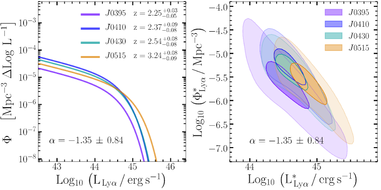
Figure 15: Left panel: single-Schechter fits to our data computed with the fixed faint-end slope $\alpha\!=\!-1.35\pm 0.84$ obtained as in Sect. 5.3.1. We note that the difference among the four determinations (factor of $\sim\!2$ both in luminosity and normalization) are absorbed by the errors on the Schechter parameters (right panel). Right panel: distribution of $\rm\Phi^{*}$ and $\rm L^{*}$ obtained from the monte-carlo sampling of $\alpha$ errors. The contours mark the levels including $86\%$ and $39\%$ of the monte-carlo realizations (respectively faint and dark contours). This analysis shows that the parameters of the four determinations are statistically consistent, hence we do not observe hints for an evolution of the $\rm 2\!\lesssim\!z\!\lesssim\!3.3$ Ly$\alpha\$LF at $\rm Log(L_{Ly\alpha}/erg\,s^{-1})\gtrsim 43.5$.

Under the hypothesis that our samples are greatly dominated by AGN/QSOs, our results show that their LF is described by a clearly distinct distribution with respect to SF LAEs (see also Matthee et al., 2017b). In particular, by comparing our $\rm\Phi^{*}$ and $\rm L^{*}$ to previous determinations at $\rm Log(L_{Ly\alpha}/erg\,s^{-1})\!<\!43$ (Gronwall et al., 2007; Ouchi et al., 2008; Konno et al., 2016), we measure a typical density and luminosity of AGN/QSOs respectively $\rm\sim\!\!3\,dex$ lower and $\rm\sim\!\!2\,dex$ higher, as already suggested by e.g. Matthee et al. (2017b) and Sobral et al. (2018b). In turn, this would suggest that the transition between the regime dominated respectively by SF LAEs and AGN/QSOs would fall at $\rm Log(L_{Ly\alpha}/erg\,s^{-1})\!\sim\!43.5$, as also highlighted by Sobral et al. (2018a) and Calhau et al. (2020).

Finally, our data do not allow to constrain the evolution of our Ly$\alpha\$LFs determinations. Indeed the $\rm\Phi^{*}$ and $\rm L^{*}$ we obtain are statistically consistent (at $\sim 2\sigma$) among the four filters, with average values $\rm\Phi^{*}\!=\!(3.33\pm 0.19)\times 10^{-6}\,Mpc^{-3}$ and $\rm L^{*}\!=\!44.65\pm 0.65\,erg\,s^{-1}$. This is shown in the right panel of Fig. 15, where the faint and dark contours for each filter respectively mark the 2-$\sigma$ and 1-$\sigma$ levels (i.e. the $\!86\%$ and $\!39\%$ iso-contours) of the parameters distributions obtained from monte-carlo realizations. The wide overlap between the four filters shows the low constraining power of our data towards the evolution of the LF parameters with redshift. This was anticipated by the significant variation among the distributions of $\rm L_{\,Ly\alpha}$ and EW at each z shown in Fig. LABEL:fig:ew_and_lyalum_distributions, which ultimately hinders the possibility to disentangle the intrinsic variations of our sample properties from systematic effects. We note that

5.4 The AGN fraction of $\rm z\!\gtrsim\!2$ LAEs

By assuming that our Ly$\alpha\$LF describes the distribution of only AGN/QSOs, we can build a simple toy model to estimate the relative fraction AGN/QSOs and SF LAEs as a function of Ly$\alpha\$luminosity. We define the latter as:

$$\rm q_{\,AGN}=\frac{LF^{\,SF\ LAEs}}{LF^{\,SF\ LAEs}+LF^{\,AGN/QSOs}}\ ,$$ (14)

where $\rm LF^{\,AGN/QSOs}$ is one of the four determinations of the Schechter function computed from our data, while $\rm LF^{\,SF\ LAEs}$ is the best fit of Sobral et al. (2018b) at the corresponding redshift. We use the latter since it is obtained by excluding LAE candidates with X-ray counterparts from the determination of the Schechter fit. Consequently, we assume it provides a fair estimate for the luminosity distribution of only SF LAEs. We underline that our estimate of $q_{\,AGN}$ is an illustrative application of our results rather than a rigorous measurement, given the strong assumptions on which it is based.

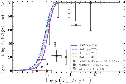
Figure 16: The AGN/QSO fraction as a function of luminosity for each NB. We estimated this quantity by assuming that our results are entirely dominated by AGN/QSOs and that the best Schechter fit of Sobral et al. (2018b) describes the distribution of SF LAEs (see Eq. 14). Our results are in agreement with the spectroscopic determination of Sobral et al. (2018a), which only employs Ly$\alpha\$emission pre-selection for their targets. On the other hand, the estimates of Matthee et al. (2017b) and Calhau et al. (2020) are based on the detection of either X-ray or radio counterparts for their Ly$\alpha\$-emitting candidates.

The AGN/QSOs fractions for all the redshifts we probe are shown in figure 16. Despite our simplifying assumptions, we find a good agreement (within $1\,\sigma$) with the measurements of Sobral et al. (2018a), which are obtained from a spectroscopic follow-up of Ly$\alpha\$-selected targets. On the contrary, the works of Matthee et al. (2017b) and Calhau et al. (2020) (also shown in Fig. 16 for comparison) are based on photometric selections which identify AGN/QSOs candidates on the basis of their X-ray and/or radio-loudness. The latter are likely to be significant only for a sub-sample of AGN/QSOs (as suggested by e.g., Sobral et al., 2018b, and Calhau et al. 2020), hence the discrepancy with our estimates might also be explained in terms of this incompleteness effect.

To conclude, the good agreement between our AGN/QSOs fraction estimates and the data of Sobral et al. (2018a) supports the scenario by which our samples are strongly dominated by Ly$\alpha\$-emitting AGN/QSOs. Furthermore, the discrepancy with respect to X-ray/Radio selected AGN candidates suggests that the latter are likely a sub-sample of the whole high-z AGN/QSOs population. Our selection, on the contrary, is only based on Ly$\alpha\$emission, hence it is likely to detect previously-unidentified high-z AGN/QSOs. This is also in line with the results of our spectroscopic follow-up program (section 3.4.2).

6 Conclusions

This work presents the determination of the bright-end of the Ly$\alpha\$luminosity function at four redshifts in the interval $\rm 2\!\lesssim z\lesssim\!3.3$, namely $\rm z\!=\!2.25^{\,+0.03}_{\,-0.05}$, $\rm z\!=\!2.37^{\,+0.09}_{\,-0.08}$, $\rm z\!=\!2.54^{\,+0.08}_{\,-0.08}$ and $\rm z\!=\!3.24^{\,+0.08}_{\,-0.09}$. We obtain the LFs by employing four lists of Ly$\alpha\$-emitting candidates selected in DR1 catalog of the J-PLUS survey, according to the significance of their photometric excess in the $J$0395, $J$0410, $J$0430 and $J$0515 narrow-bands.

We select 2547, 5556, 4994 and 1467 bright candidates ($\rm L_{Ly\alpha}>2\times 10^{\,43}\,erg\,s^{-1}$), which jointly represent the largest sample of photometric Ly$\alpha\$-emitting candidates at $\rm 2\!\lesssim z\lesssim\!3.3$ to date. We expect our lists to include both bright star-forming LAEs (SF LAEs) and Ly$\alpha\$-emitting AGN/QSOs. To identify either of these source classes in our samples, we follow-up spectroscopically a random sub-sample of our candidates (section 3.4). The spectroscopir data confirmed 40 out of 45 targets as genuine high-z line-emitters (with 29 out of 45 being $\rm z\!>\!2$ Ly$\alpha\$-emitting QSOs) and found no star-forming LAE. In addition, we look for bi-modalities in the photometric properties of our candidates, such as Ly$\alpha\$luminosity and EW (section LABEL:sec:EW_LLya_distributions) or colors (section LABEL:sec:LAE_QSOfractions). Overall, the properties of our candidates are consistent with those of spectroscopically-confirmed QSOs (Fig. LABEL:fig:color-color_candidates_and_QSOs) and high-z QSO templates (Fig. LABEL:fig:wise-color_vs_redshift), suggesting that the fraction of SF LAEs in our samples is negligible.

We use our candidates samples to compute the Ly$\alpha\$LF at extremely-bright luminosity regimes for the first time, namely at $\rm 44\!\lesssim\!Log(L_{Ly\alpha}/erg\,s^{-1})\!\lesssim\!45.5$, and extend by $\rm\gtrsim\!1.5\,dex$ the intervals covered by previous determinations. The extensive area observed by J-PLUS DR1 allows to access wide cosmological volumes ($\rm\gtrsim\!1\,Gpc^{3}$), hence to probe number densities as low as $\rm\sim\!\!10^{-8}\,Mpc^{-3}$. This parameters-space region is unprecedented for surveys focused on bright photometrically-selected Ly$\alpha\$-emitting sources. Interestingly, our Ly$\alpha\$LFs are in line with previous results at $\rm Log(L_{Ly\alpha}/erg\,s^{-1})\!\gtrsim\!43.5$, prolonging their power-law end into a full-developed Schechter function. We derive the redshift-averaged parameters $\rm\Phi^{*}\!=\!(3.33\pm 0.19)\times 10^{-6}\,Mpc^{-3}$, $\rm L^{*}\!=\!44.65\pm 0.65\,erg\,s^{-1}$ and $\rm\alpha\!=\!-1.35\pm 0.84$ for our Schechter best-fits. This shows that the whole Ly$\alpha\$LF, i.e. from $\rm Log(L_{Ly\alpha}/erg\,s^{-1})\!<\!42$ up to $\rm Log(L_{Ly\alpha}/erg\,s^{-1})\!>\!45$, can be effectively described by a composite model of two Schechter functions, respectively accounting for the distribution of SF LAEs and bright AGN/QSOs. These two distributions appear to be structurally different, with $\rm L^{*}_{QSOs}\!\sim\!100\,L^{*}_{SF\ LAEs}$, $\rm\Phi^{*}_{QSOs}\sim 10^{-3}\,\Phi^{*}_{SF\ LAEs}$ and a transition-regime centered at $\rm Log(L_{Ly\alpha}/erg\,s^{-1})\!\sim\!43.5$ (in line with e.g., Konno et al., 2016; Matthee et al., 2017b; Sobral et al., 2018a; Calhau et al., 2020). On the whole, our results support the scenario suggested by e.g. Konno et al. (2016); Matthee et al. (2017b) and Sobral et al. (2018b), according to which the excess of bright LAEs measured at $\rm Log\,\,L_{Ly\alpha}\gtrsim 43$ with respect to a Schechter distribution is due to a population of AGN/QSOs (see also Calhau et al., 2020). Our findings characterize for the first time this population as being $\rm\sim\!100$ times more luminous and $\rm\sim\!1000$ times less dense than that of SF LAEs at comparable redshifts.

In addition, $\rm\sim\!70\%$ of our Ly$\alpha\$-emitting candidates lacks any spectroscopic confirmation by current surveys. Based on our spectroscopic follow-up results, we suggest that our samples are dominated by high-z QSOs which are not yet identified as such, but rather mis-classified as stars by current archival data, due to their photometric colors. Indeed, even accounting for a conservative residual contamination of $\sim 35\%$ in our final samples, the number of genuine $\rm z\!\gtrsim\!2$ QSOs identified for the first time by our methodology would be approximately 1300, 3200, 2900 and 900, respectively for $J$0395, $J$0410, $J$0430 and $J$0515 J-PLUS NBs. We ascribe this possibility to the narrow-band excess detection of our methodology, which can be particularly effective in targeting and selecting the strong line-emission features of $\rm z\!>\!2$ AGN/QSOs. Indeed, these might be missed by spectroscopic target selection based only on broad-band colors (e.g., Richards et al., 2009; Ivezić et al., 2014; Richards et al., 2015). We stress that the confirmation of this speculative hypothesis must rely on a systematic and extensive confirmation of our candidates. The latter might be obtained via either spectroscopic analysis or by exploiting the very efficient source identification provided by multi-NB imaging. Indeed, the upcoming J-PAS survey can provide a natural setting to extend our work.

Finally, our data do not show significant evolution of the LF over the probed redshifts. Despite X-ray studies suggest little evolution of the $\rm 2\!<\!z\!<\!3.3$ AGN/QSOs population (e.g., Hasinger et al., 2007), our findings might also be affected by J-PLUS detection limits. This factor could be mitigated by deeper photometric imaging, which is hardly attainable by future J-PLUS data releases. Indeed, the technical features of the T80 (80cm) telescope hinder the possibility of reaching higher depth than the nominal J-PLUS one over very wide sky areas. On the contrary, future multi-NB wide-area photometric surveys can provide a valid tools to test the LF evolution at $\rm Log\,\,L_{Ly\alpha}\gtrsim 43.5$.

Appendix A Equations of the three-filters method

Here we derive the main equations we use to extract the integrated Ly$\alpha\$flux from J-PLUS photometry. These were originally detailed in Vilella-Rojo et al. (2015) and similar methods are described in e.g. Pascual et al. (2007) and Guaita et al. (2010). We start by defining the monochromatic flux density of an astrophysical source (or, simply, its intrinsic spectrum) as the emitted flux per unit frequency or wavelength: $\rm f_{\nu}$ or $\rm f_{\lambda}$, respectively in $\nu$-units ($\rm erg\,cm^{-2}\,s^{-1}\,Hz^{-1}$) and $\lambda$-units ($\rm erg\,cm^{-2}\,s^{-1}\,\text{\AA}\,^{-1}$). The two are connected by:

$$\rm f_{\nu}\,d\nu=f_{\lambda}\,d\lambda\quad;\quad\frac{d\nu}{d\lambda}=-\frac{c}{\lambda^{2}}\ ,$$ (15)

where c is the speed of light. In this work, we only use the $\lambda$-units formalism, although magnitudes are usually defined in terms of $\rm f_{\nu}$. Photometric measurements are usually performed through filters who probe $\rm f_{\lambda}$ over specific wavelength intervals or pass-bands. Consequently, photometric filters are defined by their transmission curves $\rm T_{\lambda}^{\,x}=T^{\,x}(\lambda)$, who describe their response as a function of wavelength. All photons received within a given pass-band during the measuring process get integrated, hence the details of $\rm f_{\lambda}$ are lost. For this reason, the flux of a source measured in a given filter “x” is effectively defined as the average flux in the pass-band weighted by the filter $\rm T_{\lambda}^{\,x}$, i.e. $\rm\left\langle f_{\lambda}^{\,x}\right\rangle$. For photon-counting devices (CCD), the latter quantity is given by (e.g., Tokunaga & Vacca 2005):

$$\rm\left\langle f_{\lambda}^{\,x}\right\rangle=\frac{\int f_{\lambda}\,T_{\lambda}^{\,x}\,\lambda\,d\lambda}{\int T_{\lambda}^{\,x}\,\lambda\,d\lambda}=\frac{\int(f_{\lambda}^{\,cont}+f_{\lambda}^{\,EL})\,T_{\lambda}^{\,x}\,\lambda\,d\lambda}{\int T_{\lambda}^{\,x}\,\lambda\,d\lambda}\ ,$$ (16)

where we assume that $\rm f_{\lambda}$ can be written as the combination of line and continuum emission (respectively $\rm f_{\lambda}^{\,EL}$ and $\rm f_{\lambda}^{\,cont}$). In order to extract the line flux from the $\rm\left\langle f_{\lambda}^{\,x}\right\rangle$ measurement, we need to disentangle $\rm f_{\lambda}^{\,EL}$ from $\rm f_{\lambda}^{\,cont}$. The equivalent width of a line measures the relative contribution of line and continuum to $\rm\left\langle f_{\lambda}^{\,x}\right\rangle$:

$$\rm EW\equiv\int_{\lambda_{min}}^{\lambda_{max}}\left|1-\frac{f_{\lambda}^{\,tot}}{f_{\lambda}^{\,cont}}\right|\,d\lambda=\int_{\lambda_{min}}^{\lambda_{max}}\left|1-\frac{f_{\lambda}^{\,cont}+f_{\lambda}^{\,EL}}{f_{\lambda}^{\,cont}}\right|\,d\lambda\ ,$$ (17)

where $\rm\lambda_{min}$ and $\rm\lambda_{max}$ encompass the whole line profile. By assuming that $\rm f_{\lambda}^{\,cont}$ is constant between $\rm\lambda_{min}$ and $\rm\lambda_{max}$, and denoting the wavelength of the line-profile peak as $\rm\lambda_{EL}$, we have:

$$\rm EW=\frac{1}{f_{\lambda_{EL}}^{\,cont}}\,\left(\int_{\lambda_{min}}^{\lambda_{max}}f_{\lambda}^{\,EL}\,d\lambda\right)\,=\,\frac{F^{\,EL}}{f_{\lambda_{EL}}^{\,cont}}\ ,$$ (18)

where $\rm f_{\lambda_{EL}}^{\,cont}=f_{\lambda}^{\,cont}(\lambda_{EL})$. This also shows the definition of the continuum-subtracted, integrated line flux $\rm F^{\,EL}$ ($\rm erg\,cm^{-2}\,s^{-1}$).

The above definitions allow to derive the basic equations of our methodology. We stress that this is designed to extract $\rm F^{\,EL}$ by using three photometric measurements (two BBs and one NB) and it is based on two main hypothesis, i) the emission-line profile can be approximated by a Dirac-delta, and ii) the source continuum is well-traced by a linear function of wavelength over the whole interval covered by the three filters (see also Sect. 3.1):

$$\rm f_{\lambda}^{\,EL}=F^{\,EL}\cdot\delta(\lambda-\lambda_{EL})\ ,$$ (19)

$$\rm f_{\lambda}^{\,cont}=A\,\lambda+B\ ,$$ (20)

where $\rm\delta(\lambda-\lambda_{EL})$ is centered at $\rm\lambda_{EL}$, while A and B are two scalar coefficients. Equation 19 implicitly assumes that $\rm F^{\,EL}$ is entirely included within the NB pass-band. This might be false when part of the emission-line profile lies outside the NB pass-band, e.g. when the line-profile is wider than the NB pass-band (as for broad QSOs lines) or its peak lies close to the NB pass-band edge. The implications of this bias on our results are discussed in Sect. LABEL:sec:line_flux_retrieval. By using 20 into 16 we get:

$$\rm\left\langle f_{\lambda}^{\,x}\right\rangle=\frac{\int(A\,\lambda+B+f_{\lambda}^{\,EL})\cdot T_{\lambda}^{\,x}\,\lambda\,d\lambda}{\int T_{\lambda}^{\,x}\,\lambda\,d\lambda}$$

$$\quad\ \ \ \,=\rm\frac{\left[A\int\lambda^{2}\,T_{\lambda}^{\,x}\,d\lambda\ +\ B\int T_{\lambda}^{\,x}\,\lambda\,d\lambda\ +\ \int f_{\lambda}^{\,EL}\,T_{\lambda}^{\,x}\,\lambda\,d\lambda\right]}{\int T_{\lambda}^{\,x}\,\lambda\,d\lambda}$$

$$\quad\ \ \ \,=\rm\frac{\left[A\int\lambda^{2}\,T_{\lambda}^{\,x}\,d\lambda\ +\ B\int T_{\lambda}^{\,x}\,\lambda\,d\lambda\ +\ F^{\,EL}\,T_{\lambda_{\,EL}}^{\,x}\,\lambda_{EL}\right]}{\int T_{\lambda}^{\,x}\,\lambda\,d\lambda},$$ (21)

where $\rm T_{\lambda_{\,EL}}^{\,x}=T_{\lambda}^{\,x}(\lambda_{EL})$, while the last step makes use of Eq. 19 in the last term at the numerator and the properties of the Dirac-delta. To simplify the notation we introduce:

$$\rm\alpha_{x}=\frac{\int\lambda^{2}\,T_{\lambda}^{\,x}\,d\lambda}{\int T_{\lambda}^{\,x}\,\lambda\,d\lambda}\quad;\quad\quad\beta_{x}=\frac{T_{\lambda_{EL}}^{\,x}\,\lambda_{EL}}{\int T_{\lambda}^{\,x}\,\lambda\,d\lambda}\ ,$$ (22)

which depend only on $\rm T^{\,x}_{\lambda}$ and $\rm\lambda_{EL}$. The latter is determined by each source redshift and cannot be measured without a spectroscopic observation, hence we must assume $\rm\lambda_{EL}$ a-priori. For each NB, we choose the value which maximizes the product $\rm T_{\lambda}\cdot[(dn/dz)\cdot(dz/d\lambda)]$, where $\rm dn/dz$ is the redshift distribution of SDSS QSOs (Pâris et al. 2018). This reflects that we expect most of our candidates to be $\rm z\!\gtrsim\!2$ QSOs, as discussed in Sect. 2.2.2 and LABEL:sec:LAE_samples. We can now re-write 21 using 22:

$$\rm\left\langle f_{\lambda}^{\,x}\right\rangle=A\cdot\alpha_{x}\ +\ B\ +\ F^{\,EL}\cdot\beta_{x}\ ,$$ (23)

which is valid for a generic filter. Note that if the targeted emission-line lies outside the pass-band we just have $\rm T_{\lambda_{EL}}^{\,x}=0$, implying $\rm\beta_{x}=0$. To determine A, B and $\rm F^{\,EL}$, we apply 23 to a set of three filters: a NB, a line-contaminated BB (denoted here by LC) and a line-uncontaminated BB (denoted by LU):

$$\rm\left\langle f_{\lambda}^{\,NB}\right\rangle=A\cdot\alpha_{NB}\ +\ B\ +\ F^{\,EL}\cdot\beta_{NB}\ ,$$ (24)

$$\rm\left\langle f_{\lambda}^{\,LC}\right\rangle=A\cdot\alpha_{LC}\ +\ B\ +\ F^{\,EL}\cdot\beta_{LC}\ ,$$ (25)

$$\rm\left\langle f_{\lambda}^{\,LU}\right\rangle=A\cdot\alpha_{LU}\ +\ B.$$ (26)

By solving this linear system we finally obtain $\rm F^{\,EL}$, A and B:

$$\rm F^{\,EL}=\frac{\left\langle f_{\lambda}^{\,LC}\right\rangle\ -\ \left\langle f_{\lambda}^{\,LU}\right\rangle\ +\ \frac{\alpha_{LU}-\alpha_{LC}}{\alpha_{NB}-\alpha_{LU}}\cdot\left[\left\langle f_{\lambda}^{\,NB}\right\rangle-\left\langle f_{\lambda}^{\,LU}\right\rangle\right]}{\beta_{LC}\ +\ \frac{\alpha_{LU}-\alpha_{LC}}{\alpha_{NB}-\alpha_{LU}}\cdot\beta_{NB}}\ ,$$ (27)

$$\rm A=\frac{\left\langle f_{\lambda}^{\,NB}\right\rangle\ -\ \left\langle f_{\lambda}^{\,LU}\right\rangle\ -\ \frac{\beta_{NB}}{\beta_{LC}}\cdot\left[\left\langle f_{\lambda}^{\,LC}\right\rangle-\left\langle f_{\lambda}^{\,LU}\right\rangle\right]}{\alpha_{NB}\ -\ \alpha_{LU}\ -\ \frac{\beta_{NB}}{\beta_{LC}}\cdot\left(\alpha_{LC}\ -\ \alpha_{LU}\right)}\ ,$$ (28)

$$\rm B=\left\langle f_{\lambda}^{\,LU}\right\rangle-\alpha_{LU}\cdot A\ .$$ (29)

The coefficients A and B can be used to evaluate 20 at the NB $\lambda$-pivot (see Tokunaga & Vacca 2005) and get an estimate of the line-uncontaminated linear continuum in the NB $\rm\left\langle f_{\lambda\,;\,cont}^{\,NB}\right\rangle$. Equation 1 in Sect. 3.1 details how we use this continuum estimate to compute the NB excess of each J-PLUS source. Finally, we use Eq. 27 to estimate the total line flux of our LAE candidates and construct their LFs as explained in Sect. LABEL:sec:lumifunc.

Appendix B Measurement of GTC spectra and follow-up results

We measure the redshift of all the 37 sources identified as QSOs (either at $\rm z\!\sim\!1.5$ or at $\rm z\!\sim\!2.2$) in both spectroscopic programs. We do not aim at reaching a higher precision than $\rm\sigma_{z}=10^{-2}$, since the main goal of our follow-up programs is the spectroscopic confirmation of our targets. We additionally extract the Ly$\alpha\$EW and integrated line flux $\rm F_{Ly\alpha}$ for the 29 $\rm z\!\sim\!2.2$ QSOs, from which we compute the sources Ly$\alpha\$luminosity.

Following well-established procedures (see e.g., Pâris et al. 2011), we first identify the main spectral lines in our QSOs spectra, such as CIV and CIII]. We then use their profile-peaks to compute our redshift estimate. We discard the Ly$\alpha\$profile for this analysis, since it provides a systematically biased z measure, due to the complex radiative transfer of Ly$\alpha\$photons in the source rest frame and IGM (see e.g., Gronke et al. 2016; Dijkstra 2017; Gurung-Lopez et al. 2018). We fit a double gaussian profile to both CIV and CIII] profiles, in order to trace at the same time its broad and narrow components. We use the $\lambda$ position of the narrow-component peaks to obtain two z estimates, whose average provides the final spectroscopic z of our sources.

Figure 17: Calibrated spectrum (grey solid line) of the GTC2018A_09 target, confirmed as $\rm z\!\sim\!2.2$ QSO. The four green regions highlight the intervals used for computing the power-law fit to the continuum (dashed yellow line). Finally, the Ly$\alpha\$integrated flux is highlighted in red.

The Ly$\alpha\$line flux can only be obtained after estimating the sources continua. We then fit a power law to the wavelength regions of each spectrum which are not affected by any line feature, as shown by the yellow sections of the spectrum displayed in Fig. 17. We use the following simple functional form:

$$\rm f_{\lambda}^{\,c}(\lambda)=k\,\lambda_{obs}^{\,\alpha}\ ,$$ (30)

where $\rm f_{\lambda}^{\,c}(\lambda)$ is the spectrum monochromatic flux density (in units of $\rm erg\,cm^{-2}\,s^{-1}\,\text{\AA}^{-1})$) while $\rm k$ and $\alpha$ are fit parameters. Finally, we measure the total Ly$\alpha\$line flux by integrating the excess above the estimated continuum in the wavelength range affected by the Ly$\alpha\$line, which is shown in Fig. 17 as the spectral region highlighted in dark-red. As a last step, we estimate the observed Ly$\alpha\$EW as:

$$\rm EW_{obs}^{Ly\alpha}=\frac{F_{Ly\alpha}}{\rm f_{\lambda}^{\,c}(\lambda_{Ly\alpha})}\ ,$$ (31)

in which $\rm f_{\lambda}^{\,c}(\lambda_{Ly\alpha})$ is the value of the power-law fit to the continuum at the wavelength of the Ly$\alpha\$line-profile peak. Figure 17 shows the spectrum of target GTC2018A_09 as a visual example of our measuring procedure. The results of these measurements are shown in Table 8 together with a summary of the spectroscopic follow-up thechnical requrements and additional properties of the observed targets.

Instrument	OSIRIS spectrograph at Gran Telescopio Canarias (GTC)
Grism	R500B
Seeing	requested: 1.4 (maximum) — effective: 1.03 (averaged on all observations)
Moon	requested: any — effective: $>\!90$% Dark
Air mass	requested: 1.5 (maximum) — effective: 1.266 (averaged on all observations)
SNR	$\rm\geqslant 3$ at $\rm\lambda_{obs}\sim 4000\text{\AA}$
ID	Ra [hh:mm:ss]	Dec [hh:mm:ss]	Time [s]	SDSS class	GTC class	$\rm\mathbf{z_{\,spec}}$	$\rm\mathbf{L_{Ly\alpha}}$	$\rm\mathbf{EW_{obs}}$
GTC2018A_01	22:50:40.27	34:23:43.6	2185	—	QSO/AGN	2.21	5.18e+44	513.98
GTC2018A_02	00:43:38.56	05:41:35.6	2185	GALAXY	QSO/AGN	2.23	1.70e+44	417.21
GTC2018A_03	23:01:08.05	33:44:20.0	2185	STAR	STAR	—	—	—
GTC2018A_04	16:17:15.12	50:25:59.2	2185	STAR	QSO/AGN	1.52	—	—
GTC2018A_05	22:22:06.30	11:07:47.7	2335	STAR	QSO/AGN	2.23	3.87e+43	268.21
GTC2018A_06	18:10:22.34	41:49:25.3	2185	STAR	QSO/AGN	2.22	2.32e+44	741.21
GTC2018A_07	17:35:17.03	31:44:42.8	2185	GALAXY	QSO/AGN	2.23	7.46e+43	665.04
GTC2018A_08	01:31:29.69	33:55:14.9	2185	STAR	QSO/AGN	2.21	1.26e+44	637.59
GTC2018A_09	14:59:37.24	47:15:26.3	2185	STAR	QSO/AGN	2.18	2.13e+44	502.01
GTC2018A_10	16:11:57.72	46:00:45.8	2185	STAR	QSO/AGN	2.21	1.56e+44	263.97
GTC2018A_11	18:32:04.26	39:54:08.8	2185	—	QSO/AGN	1.54	—	—
GTC2018A_12	02:16:13.21	34:28:37.3	2185	—	QSO/AGN	2.21	1.33e+44	272.11
GTC2018A_13	14:32:51.07	52:36:46.7	1954	GALAXY	GALAXY	0.51	—	—
GTC2018A_14	22:01:43.81	28:23:36.5	2335	STAR	QSO/AGN	1.53	—	—
GTC2018A_15	16:09:37.67	45:29:53.6	2245	STAR	STAR	—	—	—
GTC2018A_16	22:43:00.76	34:10:26.4	2335	STAR	QSO/AGN	2.25	—	—
GTC2018A_17	15:59:27.15	57:05:04.6	2245	STAR	QSO/AGN	2.22	1.08e+44	268.69
GTC2018A_18	23:03:24.69	33:20:25.5	2245	STAR	STAR	—	—	—
GTC2018A_19	16:03:33.14	46:11:53.2	2245	—	QSO/AGN	2.25	6.19e+43	351.25
GTC2018A_20	15:19:49.02	53:16:18.4	2335	STAR	QSO/AGN	2.19	2.04e+44	828.73
GTC2018A_21	14:53:19.08	53:02:42.3	2365	STAR	QSO/AGN	2.19	6.15e+43	217.99
GTC2018A_22	17:41:33.43	57:05:11.4	2335	STAR	QSO/AGN	2.27	8.20e+43	481.13
GTC2018A_23	15:38:49.50	48:58:13.1	2014	GALAXY	STAR	—	—	—
GTC2018A_24	14:53:32.94	54:09:44.8	2335	GALAXY	QSO/AGN	1.53	—	—
GTC2019A_01	07:18:49.01	40:50:42.7	1165	STAR	STAR	—	—	—
GTC2019A_02	22:37:58.84	11:41:01.4	1285	STAR	QSO/AGN	2.204	4.56e+44	706.71
GTC2019A_03	02:27:21.78	29:56:23.7	1366	STAR	QSO/AGN	2.202	3.41e+44	859.82
GTC2019A_04	16:14:11.38	53:11:16.6	1426	STAR	BAL QSO	2.174	2.79e+44	290.75
GTC2019A_05	15:31:12.21	48:08:31.4	1576	STAR	QSO/AGN	2.209	2.91e+44	570.59
GTC2019A_06	15:34:37.75	46:42:36.3	1816	STAR	QSO/AGN	2.231	3.02e+44	414.59
GTC2019A_07	12:38:36.94	56:10:39.8	2086	STAR	QSO/AGN	2.177	2.02e+44	183.25
GTC2019A_08	12:29:07.02	56:03:49.2	2086	STAR	QSO/AGN	2.191	1.35e+44	230.15
GTC2019A_09	08:03:53.42	30:46:36.2	2206	STAR	QSO/AGN	2.256	2.14e+44	380.86
GTC2019A_10	07:15:23.13	39:50:57.3	2356	STAR	QSO/AGN	2.189	1.29e+44	625.73
GTC2019A_11	09:00:47.61	32:06:54.9	2806	GALAXY	QSO/AGN	2.253	9.54e+43	364.01
GTC2019A_12	00:51:10.29	03:08:25.4	3406	STAR	QSO/AGN	1.543	8.34e+43	104.21
GTC2019A_13	17:25:01.20	33:46:50.4	3706	STAR	QSO/AGN	1.602	1.27e+44	180.52
GTC2019A_14	10:28:20.14	39:52:42.3	3706	STAR	QSO/AGN	2.271	1.83e+44	121.36
GTC2019A_15	00:32:08.19	39:47:23.6	4476	STAR	QSO/AGN	1.512	1.33e+44	118.74
GTC2019A_16	16:14:30.92	50:12:24.2	4686	GALAXY	QSO/AGN	2.211	1.00e+44	705.82
GTC2019A_17	00:41:06.77	08:02:56.5	4761	STAR	GALAXY	—	—	—
GTC2019A_18	16:10:19.83	45:31:49.4	5136	GALAXY	QSO/AGN	2.271	1.06e+44	644.06
GTC2019A_19	22:56:29.07	09:36:45.5	5136	STAR	QSO/AGN	2.762	8.96e+43	390.88
GTC2019A_20	09:10:21.90	38:39:30.6	6246	GALAXY	QSO/AGN	1.528	1.61e+44	561.05
GTC2019A_21	13:20:29.68	56:31:49.6	6795	GALAXY	QSO/AGN	2.197	8.61e+43	154.68

Table 8: Properties retrieved from the follow-up of our 45 spectroscopic targets. These results confirm $29/45$ sources ($64.4\%$) as genuine Ly$\alpha\$-emitting QSOs at $\rm z\!\sim\!2$. The most numerous interlopers are CIV-emitting QSOs at $\rm z\!\sim\!1.52$, namely $8/45$ targets ($\sim 18\%$, see Stroe et al. 2017a, b), and $5/45$ blue stars ($\sim 11\%$). The latter are selected by our pipeline due to their strong color-gradients which mimic a NB photometric excess in the $J$0395 filter. We also note one $\rm Ly\beta$-emitting QSO contaminant at $\rm z\!\sim\!2.76$. We report the measured $\rm L_{Ly\alpha}$ and $\rm EW_{obs}$ only for the confirmed QSOs at $\rm z\!\sim\!2.2$. Among these, the spectrum of GTC 16 could not be calibrated and measured.Finally, all the $\rm z\!\sim\!2.2$ confirmed sources in our sample are QSOs with $\rm L_{Ly\alpha}\!>\!6\times 10^{43}\,erg\,s^{-1}$. This supports the results of Konno et al. (2016); Matthee et al. (2017b); Sobral et al. (2018a, b) and Calhau et al. (2020) about the strong contribution of AGN/QSOs to the Ly$\alpha\$LF at $\rm Log(Ly\alpha)\!\gtrsim\!43.3$.

Appendix C Retrieval of the total line flux

Here we describe how we characterize and correct the bias on our measurements of Ly$\alpha\$flux (namely $\rm F^{\,3FM}_{Ly\alpha}$). We compute a correction for each NB by exploiting the comparison between J-PLUS sources and their counterparts in the SDSS QSOs catalog (Pâris et al. 2018), within the redshift windows sampled by the NB. For the sake of brevity, we only show the results for either $J$0410 or $J$0430 filters. As a first step, we introduce the Ly$\alpha\$flux quantities obtained from SDSS spectra in order to perform our comparison (see Fig. 18):

• $\rm\langle\mathit{f}^{\,x}_{\lambda}\rangle^{synth}\,$: synthetic flux-density, in $\rm erg\,cm^{-2}\,s^{-1}\,\text{\AA}^{-1}$, measured by convolving SDSS spectra with the transmission curve of a given J-PLUS filter “x”, as in eq. 16. Coloured crosses in the bottom panel of Fig. 18 mark the synthetic photometry of the SDSS QSO taken as example.

• $\rm F^{\,spec}_{Ly\alpha}$: spectroscopic measurement of the wavelength-integrated Ly$\alpha\$flux, in $\rm erg\,cm^{-2}\,s^{-1}$. This is obtained by fitting the QSOs continuum and integrating the spectra above it, on the wavelength range affected by the whole Ly$\alpha\$line profile (see appendix B for details). This measurement does not involve the convolution of SDSS spectra with the filters transmission curves.

• $\rm F^{\,spec\,;\,NB}_{Ly\alpha}$: a version of $\rm F^{\,spec}_{Ly\alpha}$ obtained by integrating the spectra above the continuum-fit exclusively over the wavelength range covered by a J-PLUS NBs. If the Ly$\alpha\$line of a given QSO is wider than the NB, this measurement is just a fraction of $\rm F^{\,spec}_{Ly\alpha}$, since the Ly$\alpha\$flux lying outside the transmission curve would not be accounted for (see Fig. 18).

• $\rm F^{\,3FM\,;\,synth}_{Ly\alpha}$: this photometric quantity is analogous to $\rm F^{\,3FM}_{Ly\alpha}$, with the only difference of being computed on the synthetic photometry of SDSS QSOs (coloured crosses in the bottom panel of Fig. 18).

The photometric quantity $\rm F^{\,3FM}_{Ly\alpha}$ is directly comparable to the spectroscopic $\rm F^{\,spec;\,NB}_{Ly\alpha}$, since the method of Vilella-Rojo et al. (2015) is designed to remove the effect of the filter transmission curve (see also appendix A). Moreover, any photometric measurement is only sensitive to the flux received within a given band, hence to $\rm F^{\,spec;NB}_{Ly\alpha}$ and not to $\rm F^{\,spec}_{Ly\alpha}$, in our case.

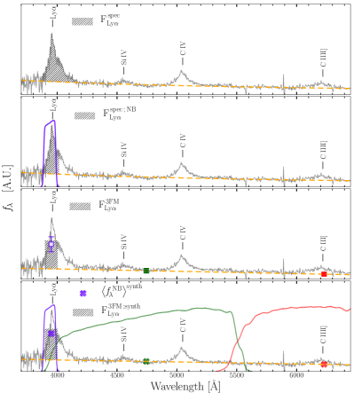
Figure 18: Graphic definition of the quantities we use for comparing Ly$\alpha\$flux. The spectrum of a $\rm z\!\sim\!2.2$ QSO from SDSS DR14 is used as example in all panels (grey lines). Each Ly$\alpha\$flux definition is outlined by a grey shaded area (see text for details). Yellow lines in each panel show the reconstruction of the source continuum (power-law and linear approximation respectively in the first two and last two panels from above). Finally, colored squares and crosses (respectively third and last panel from the top) show respectively J-PLUS measurements and synthetic photometry performed on the SDSS spectrum with J-PLUS transmission curves (Eq. 16).

C.1 $r$-band auto-aperture flux

Figure 19 shows the comparison between $r$-band flux and $\rm\langle\mathit{f}^{\,\,\mathit{r}}_{\lambda}\,\rangle^{\,synth}\,$ for J-PLUS sources and their QSOs counterparts with Ly$\alpha\$in the $J$0410 filter. The left panel displays no systematic shift, hence no strong aperture bias ($\lesssim 0.2\,\sigma_{r}$) affects the auto-aperture flux of point-like sources. Since $\rm z\!\gtrsim\!2$ sources appear point-like in J-PLUS (see Sect. 2.2.3), we conclude that auto-aperture photometry collects the total light of our Ly$\alpha\$-emitting candidates. On the other hand, the spread of the distribution in the right panel is significantly greater than one, hence we need to account for this additional statistic uncertainty on top of J-PLUS photometric errors when computing $\rm F^{\,3FM}_{Ly\alpha}$. We re-scale the photometric errors of $r$ band photometry and propagate the resulting $\sigma_{r}$ on $\rm F^{\,3FM}_{Ly\alpha}$. The latter is accounted for in the errors of our LFs as discussed in Sect. LABEL:sec:errors_on_the_LF.

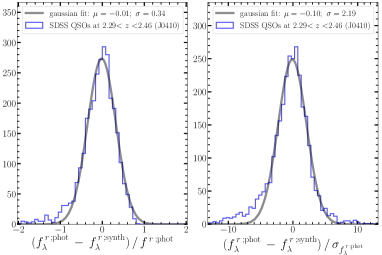
Figure 19: Blue solid lines in both panels show the histograms of the difference between J-PLUS $r$ flux (i.e. $\rm\mathit{f}_{\lambda}^{\,\mathit{r}}$) and $\rm\mathit{f}^{\,\mathit{r}\,;\,synth}_{\lambda}$ obtained from SDSS QSOs spectra (see Fig. 18). The distributions are normalized by respectively $\rm\mathit{f}_{\lambda}^{\,\mathit{r}}$ (left panel) and its photometric error $\rm\sigma_{\mathit{f}_{\lambda}^{\,\mathit{r}}}$ (right panel). Both distributions are centered in zero (see plot legends), meaning that $\rm\mathit{f}_{\lambda}^{\,\mathit{r}}$ and $\rm\mathit{f}^{\,\mathit{r}\,;\,synth}_{\lambda}$ values are statistically equivalent. On the other hand, the distribution spread in the right panel is significantly bigger than one, hence photometric errors do not fully account for the flux difference. Consequently, we re-scale $\rm\sigma_{\mathit{f}_{\lambda}^{\,\mathit{r}}}$ to the value obtained by the Gaussian fit (right-panel legend).

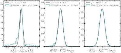
Figure 20: Cyan solid lines in all panels show the histograms of differences between line flux measurements performed on J-PLUS photometry (section 3.1) and on SDSS spectroscopy (Fig. 18), for the case of $J$0430. The difference between $\rm F^{\,3FM}_{Ly\alpha}$ and $\rm F^{\,spec}_{Ly\alpha}$ is normalized respectively by $\rm F^{\,3FM}_{Ly\alpha}$ and by $\rm\sigma_{F^{\,3FM}_{Ly\alpha}}$ in the left and middle panels. We use the systematic shift of the distributions in the left panel to statistically correct $\rm F^{\,3FM}_{Ly\alpha}$, while the distribution spread in the middle panel allows to account for residual statistical errors not included in $\rm\sigma_{F^{\,3FM}_{Ly\alpha}}$. Section LABEL:sec:errors_on_the_LF details how the systematic offset (left panel) and distribution spread (middle panel) concur to the errors on our final LFs. Finally, right panel shows that $\rm F^{\,3FM}_{Ly\alpha}$ well compares to the spectroscopic measure $\rm F^{\,spec\,;\,NB}_{Ly\alpha}$.

C.2 Filter-width effect on the line flux

Since the observed Ly$\alpha\$line profile of QSOs is generally wider than the FWHM of J-PLUS NBs, we need to account for line-flux losses. For this, we obtain two corrections, respectively for $\rm F^{\,3FM}_{Ly\alpha}$ and its errors $\rm\sigma_{F^{\,3FM}_{Ly\alpha}}$. These affect the Ly$\alpha\$luminosity of our candidates and its errors, hence we account for them on our final LFs (as discussed in Sect. LABEL:sec:errors_on_the_LF). Figure 20 shows the comparison between $\rm F^{\,3FM}_{Ly\alpha}$ and $\rm F^{\,spec}_{Ly\alpha}$ for $J$0430 filter. Their flux-difference is presented in the left and middle panel, respectively normalized by $\rm F^{\,3FM}_{Ly\alpha}$ and by $\rm\sigma_{F^{\,3FM}_{Ly\alpha}}$. The left panel shows clear evidences of a systematic offset $\rm\Delta F$ between the two flux quantities. We measure $\rm\Delta F$ with a gaussian fit (see Fig. 20) and use it to correct $\rm F^{\,3FM}_{Ly\alpha}$ as follows:

$$\rm F^{\,3FM\,;\,corr}_{Ly\alpha}=(1-\Delta F)\cdot F^{\,3FM}_{Ly\alpha}\ .$$ (32)

We stress that by directly comparing $\rm F^{\,3FM}_{Ly\alpha}$ to $\rm F^{\,spec}_{Ly\alpha}$, our statistical correction accounts for any systematic bias of our measurements, such as the linear-continuum approximation or the line-peak position of Ly$\alpha\$within the NB. The spread of the distribution in the middle panel of Fig. 20 is significantly bigger than unity. This shows that $\rm\sigma_{F^{\,3FM}_{Ly\alpha}}$ cannot fully account for the difference between $\rm F^{\,3FM}_{Ly\alpha}$ and $\rm F^{\,spec}_{Ly\alpha}$. Consequently, we re-scale $\rm\sigma_{F^{\,3FM}_{Ly\alpha}}$ according to the measured spread of the distribution in the middle panel of Fig. 20. Finally, we account for these errors on our final LFs (see Sect. LABEL:sec:errors_on_the_LF). To conclude, the comparison between middle and right panels of Fig. 20 clearly shows how $\rm F^{\,3FM}_{Ly\alpha}$ better compares to the fraction of spectroscopic line-flux measured only on the wavelength range covered by the J-PLUS NB (i.e. $\rm F^{\,spec\,;\,NB}_{Ly\alpha}$, see Fig. 18 and Sect. C). This is a direct effect of the filter-width bias, because our methodology is only sensitive to the flux captured by J-PLUS photometry within the NB wavelength range, as discussed in Sect. C.

Appendix D Multi-variate completeness computation

Here we describe the computation of the corrections accounting for incompleteness due to our selection methodology (section D.1) and the use of $r$-band detected catalogs (section D.2).

D.1 Selection completeness

To simplify, our selection depends on i) the linear approximation of the sources continuum, ii) their Ly$\alpha\$flux and iii) their Ly$\alpha\$EW. To account for these dependencies, we measure the recovery rate of our methodology as a function of i) $g\!-\!r$ color, ii) Ly$\alpha\$flux and iii) $r$-band magnitude. Indeed, $g\!-\!r$ color can be thought as a proxy of our linear continuum approximation (see e.g. Fig. 2), hence the EW dependence of our selection is accounted for by independently varying the Ly$\alpha\$flux with respect to $g\!-\!r$ and $r$ magnitude. More in detail:

1. we first subtract the measured $\rm F^{\,3FM}_{Ly\alpha}$ from the sources photometry of our candidates, in order to get a list of non-emitters, i.e. sources without a significant NB excess according to our measuring method,

2. then we artificially re-add increasing values of line flux to the sources photometry (i.e. to the NB and the $g$ band, since both are affected by the emission line),

3. for each value of the re-added flux, we apply our complete set of selection rules (section 3.2) and we store the number of re-selected sources as a function of their $r$ magnitude and $g-r$ color,

4. we finally compute the sources-recovery rate of our selection as $\rm C=N_{selected}/N_{total}$ in each bin of $r$ magnitude, $g-r$ color and artificially-injected Ly$\alpha\$flux.

With this method we obtain a 3D grid of recovery rates which can be interpolated in order to compute a selection weight $\rm C^{\,s}_{i}$ for each source. The latter accounts for the loss of candidates due to our selection within the total completeness correction we apply to the final LFs. The computation of $\rm C^{\,s}_{i}$ depends on Ly$\alpha\$-flux since this is the observable tackled by our measuring method (see e.g. Sect. 3.1 and A). Nevertheless, this dependence can be directly converted into a $\rm L_{Ly\alpha}$ dependence by assuming a redshift for every source (see Sect. LABEL:sec:lyalum_and_volume_computation). Figure 21 shows the recovery-rates grid for $J$0430 filter as an examples. The values are projected in the planes $\rm F_{Ly\alpha}$ vs. $r$ (left panel) and $\rm F_{Ly\alpha}$ vs. $g\!-\!r$ (right panel).

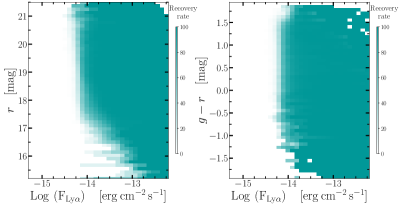
Figure 21: 3D grid of recovery rates for the $J$0430 filter, taken as example. Left and right panels respectively show the projections of recovery rates in the Ly$\alpha\$flux vs. $r$ plane and Ly$\alpha\$flux vs. $g\!-\!r$ plane. We note that the recovery rates show noisy values at $r\!<\!17$ and $g\!-\!r\!<\!-1.25$ due to the low number of sources in these magnitude and color bins. Nevertheless, these regions of the 3D parameter space are excluded from the LF computation by the purity weight (section LABEL:sec:purity_of_samples).

D.2 Bivariate completeness model

Since we use $r$-band detected catalogs, we need to take into account the loss of undetected continuum-faint Ly$\alpha\$-emitting sources. In other words, we need to estimate the distribution of sources in regions of the $\rm L_{Lya}$ vs. $r$ plane which lie outside the thresholds on $r$ and NB-excess significance imposed by J-PLUS detection limits. To carry out this analysis we closely follow the methods of Gunawardhana et al. (2015), who tackled a very similar issue with a multi-variate approach. More in detail, we build the bivariate luminosity function of our candidates, defined as the number density of sources in each bin of $\rm Log\,(L_{Ly\alpha})$ and $r$, weighted by the purity and completeness corrections:

$$\rm\Phi[\,Log\,(L_{Ly\alpha}),\,\mathit{r}\,]_{\,j\,k}\,=\,\frac{\sum_{i}\ [P_{i}\,/\,(C^{\,d}_{i}\cdot C^{\,s}_{i})]}{V\ \cdot\,\Delta_{j}\,Log(L_{Ly\alpha})\ \cdot\,\Delta_{k}\mathit{r}}\ ,$$ (33)

where j and k indexes identify the 2D bins of $\rm Log(L_{Ly\alpha})$ and $r$, while the index i runs over the total number of sources in each 2D bin. $\rm P_{i}$ is the purity weight of each candidate (see Sect. LABEL:sec:purity_of_samples), while $\rm C^{\,d}_{i}$ and $\rm C^{\,s}_{i}$ are respectively its detection-completeness (section LABEL:sec:detection_completeness) and selection-completeness (section LABEL:sec:flux_completeness and appendix D.1) weights. Finally, $\rm V$ is the survey effective volume for a given NB filter (see Sect. LABEL:sec:lyalum_and_volume_computation and Table 2). By following Gunawardhana et al. (2015), we assume that the 2D LF can be modelled by the product of two functions, describing respectively the $r$ and $\rm Log(L_{Ly\alpha})$ distributions (see also Corbelli et al. 1991). We choose to employ the combination of a Schechter function (in logaritmic form) for $r$ and a Gaussian in $\rm Log\,L_{Ly\alpha}$ (as in Gunawardhana et al. 2015):

$$\begin{array}[]{l}\rm\Phi(\mathit{r})=0.4\ ln(10)\ \Phi_{\,r}^{*}\ 10^{\,0.4(\,r^{*}\,-\,r\,)(\alpha_{\,r}+1)}\ exp[-10^{0.4(\,r^{*}\,-\,r\,)}]\vspace{2mm}\\ \rm\Phi(LogL)=\frac{\Phi_{L}^{*}}{\sigma_{L}\,\sqrt{2\pi}}\,exp\left[-\frac{1}{2\,\sigma_{L}^{2}}\,\left(LogL\,-\,LogL^{*}\right)^{2}\right]\ ,\end{array}$$ (34)

where $\rm\Phi_{r}^{*}$, $\rm r^{*}$, $\rm\alpha_{r}$ are the ordinary Schechter parameters (see Schechter 1976), while $\rm\Phi_{L}^{*}$, $\rm L^{*}$, $\rm\sigma_{L}$ describe respectively the number-density normalization, the average luminosity and the spread of the $\rm L_{Ly\alpha}$ distribution in each $r$ bin. In order to obtain the bivariate model, we follow Gunawardhana et al. (2015) and join the two univariate distributions presented in Eq. 34 with an equation between their structural parameters:

$$\rm L^{*}(\mathit{r})=10^{\,A\,(r\,-\,r_{0}^{*})\,+\,B}\ ,$$ (35)

where A and B are free parameters to be determined by fitting the 2D model to our data, while $\rm r_{0}^{*}=19.5$ (as in Gunawardhana et al. 2015). By substituting Eq. 35 into 34 and multiplying the two univariate distributions, we obtain the full bivariate model:

$$\begin{array}[]{l}\rm\Phi[\,Log\,(L_{Ly\alpha}),\,\mathit{r}\,]=\rm\Phi(\mathit{r})\,\times\,\Phi(LogL_{Ly\alpha}\,;\,\mathit{r})=\vspace{2mm}\\ \rm 0.4\ \,ln(10)\ \,\Phi_{\,r}^{*}\ \,10^{\,0.4(\,r^{*}\,-\,r\,)(\alpha_{\,r}+1)}\ \,\rm exp\left[-10^{0.4(\,r^{*}\,-\,r\,)}\right]\ \,\times\vspace{2mm}\\ \rm\frac{\Phi_{L}^{*}}{\sigma\,\sqrt{2\pi}}\,exp\left\{-\frac{1}{2\,\sigma^{2}}\,\left[LogL\,-\,\left(A\,(r\,-\,r_{0}^{*})\,+\,B\right)\right]^{2}\right\}\ .\end{array}$$ (36)

We fit the seven free parameters of this function using our measured 2D luminosity function. In particular, we only use the candidates with a completeness weight $\rm(C^{\,d}_{i}\cdot C^{\,s}_{i})\!>\!0.85$, in order to avoid biasing our fit with regions affected by the incompleteness of our selection. Finally, the ratio between the measured 2D LF of our candidates and the fitted model (over the whole $r$ - $\rm L_{Ly\alpha}$ plane) provides an estimate of the incompleteness of our selection in each $\rm[Log(L_{Ly\alpha}),\mathit{r}]$ bin. We use this ratio to compute a bivariate weight $\rm C^{\,b}_{i}$ for each of our candidates. These weights are then combined to $\rm C^{\,d}_{i}$ and $\rm C^{\,s}_{i}$ in order to obtain our total completeness correction (see Sect. LABEL:sec:completeness).