Nearest Neighbour Based Estimates of Gradients:
Sharp Nonasymptotic Bounds and Applications

Abstract

Motivated by a wide variety of applications, ranging from stochastic optimization to dimension reduction through variable selection, the problem of estimating gradients accurately is of crucial importance in statistics and learning theory. We consider here the classic regression setup, where a real valued square integrable r.v. $Y$ is to be predicted upon observing a (possibly high dimensional) random vector $X$ by means of a predictive function $f(X)$ as accurately as possible in the mean-squared sense and study a nearest-neighbour-based pointwise estimate of the gradient of the optimal predictive function, the regression function $m(x)=\mathbb{E}[Y\mid X=x]$. Under classic smoothness conditions combined with the assumption that the tails of $Y-m(X)$ are sub-Gaussian, we prove nonasymptotic bounds improving upon those obtained for alternative estimation methods. Beyond the novel theoretical results established, several illustrative numerical experiments have been carried out. The latter provide strong empirical evidence that the estimation method proposed works very well for various statistical problems involving gradient estimation, namely dimensionality reduction, stochastic gradient descent optimization and quantifying disentanglement.

1 Introduction

In this paper, we place ourselves in the usual regression setup, one of the flagship predictive problems in statistical learning. Here and throughout, $(X,Y)$ is a pair of random variables defined on the same probability space $(\Omega,\;\mathcal{F},\;\mathbb{P})$ with unknown probability distribution $P$: the r.v. $Y$ is real valued and square integrable, whereas the (supposedly continuous) random vector $X$ takes its values in $\mathbb{R}^{D}$, with $D\geq 1$, and models some information a priori useful to predict $Y$. Based on a sample $\mathcal{D}_{n}=\{(X_{1},Y_{1}),\;\ldots,\;(X_{n},Y_{n})\}$ of $n\geq 1$ independent copies of the generic pair $(X,Y)$, the goal pursued is to build a Borelian mapping $f:\mathbb{R}^{d}\rightarrow\mathbb{R}$ that produces, in average, a good prediction $f(X)$ of $Y$. Measuring classically its accuracy by the squared error, the learning task then boils down to finding a predictive function $f$ that is solution of the risk minimization problem $\min_{f}\mathcal{R}_{P}(f)$, where

$$\mathcal{R}_{P}(f)=\mathbb{E}\left[\left(Y-f(X)\right)^{2}\right].$$ (1)

Of course, the minimum is attained by the regression function $m(X)=\mathbb{E}[Y\mid X]$, which is unknown, just like $Y$’s conditional distribution given $X$ and the risk (1). The empirical risk minimization (ERM) strategy consists in solving the optimization problem above, except that the unknown distribution $P$ is replaced by an empirical estimate based on the training data $\mathcal{}D_{n}$, such as the raw empirical distribution $\hat{P}_{n}=(1/n)\sum_{i\leq n}\delta_{X_{i}}$ typically, denoting by $\delta_{x}$ the Dirac mass at any point $x$, and minimization is restricted to a class $\mathcal{F}$ supposed to be rich enough to include a reasonable approximant of $m$ but not too complex (e.g. of finite VC dimension) in order to control the fluctuations of the deviations between the empirical and true distributions uniformly over it. Under the assumption that the random variables $Y$ and $f(X)$, $f\in\mathcal{F}$, have sub-Gaussian tails, the analysis of the performance of empirical risk minimizers (i.e. predictive functions obtained by least-squares regression) has been the subject of much interest in the literature, see e.g. Györfi et al. (2002), Massart (2007), Boucheron et al. (2013) or Lecué and Mendelson (2016) (and refer to e.g. Lugosi and Mendelson (2016) for alternatives to the ERM approach in non sub-Gaussian situations).

In this paper, we are interested in estimating accurately the (supposedly well-defined) gradient $\nabla m(x)$ by means of the popular $k$ nearest neighbour ($k$-NN) approach, see e.g. Chapter in Devroye et al. (1996) or Biau and Devroye (2015). The gradient learning issue has received increasing attention in the context of local learning problems such as classification or regression these last few years, see e.g. Mukherjee and Wu (2006); Mukherjee and Zhou (2006). Because it provides a valuable information about the local structure of a dataset in a high-dimensional space, an accurate estimator of the gradient of a predictive function can be used for various purposes such as dimensionality reduction or variable selection (see e.g. Hristache et al. (2001, 1998); Xia et al. (2002); Xia (2007); Dalalyan et al. (2008); Ye and Xie (2012)), the partial derivative w.r.t. a given variable being a natural indicator of its importance regarding prediction. The previous references are all concerned with outer-products of gradients so as to recover some dimension-reduction subspace. Estimators of the gradients have also been proposed for zeroth-order optimization (see e.g. Wang et al. (2018)) and can benefit from good convergence properties.

Whereas the use of standard nonparametric methods for gradient estimation is documented in the literature (see (Fan and Gijbels, 1996; Delecroix and Rosa, 1996; De Brabanter et al., 2013) for the use of local-polynomial with kernel smoothing techniques, (Gasser and Müller, 1984) for the so-called Gasser-Muller alternative and (Zhou and Wolfe, 2000) for the use of regression spline), it is the purpose of the present article to investigate the performance of an alternative local averaging method, the popular $k$-NN method. As it provides piecewise constant estimates, it is easier to conceptualize for the practitioner and, more importantly; the neighbourhoods determined by the parameter $k$ are data-driven and often more consistent than those defined by the bandwidth in the kernel setting, especially in high dimensions.

Here we investigate the behaviour of the estimator of the (supposedly sparse) gradient of the regression function at a given point $x\in\mathbb{R}^{D}$, obtained by solving a regularized local linear version of the $k$-NN problem with a Lasso penalty. Precisely, nonasymptotic bounds for the related estimation error are established. Whereas $k$-NN estimators of the regression function have been extensively analysed from a nonasymptotic perspective (see e.g. Jiang (2019) and the references therein), the result stated in this paper is the first of this type to the best of our knowledge.

The relevance of the approach promoted is then illustrated by several applications. A variable selection algorithm that exploits the local nature of the gradient estimator proposed is first exploited to refine the popular random forest algorithm (see Breiman (2001)): by exploiting the node estimate of the gradient we are able to better direct the choice of cuts. Very simple to implement and accurate, as supported by the various numerical experiments carried out, it offers an attractive and flexible alternative to existing traditional methods such as PCA or the more closely related method of Dalalyan et al. (2008), allowing for a local reduction of the dimension rather than implementing a global preprocessing of the data. We next show how a rough statistical estimate of the gradient of any smooth objective function based on the estimation principle previously analysed in the context of regression can be exploited in a basic gradient descent algorithm, we exploit the local structure of the algorithm to be able to reuse past computations in order to calculate our estimator and jump to a better local minimum at each gradient step as well. Finally, we give an example of the usefulness of a sparse gradient estimate when one believes the gradient to be truly sparse: we use our estimator to retrieve the direction of interest for a specific attribute inside a disentangled representation and show how this can be used as an ad hoc measure of disentanglement.

The article is organized as follows. In section 2, the estimation method and the assumptions involved in the subsequent analysis are listed. The main theoretical results of the paper are stated in section 3, while several applications of the estimation method promoted are described at length and illustrated by numerical experiments in section 4. Some concluding remarks are collected in section 5 and technical proofs, as well as additional numerical results, are postponed to the Supplementary Material.

2 Background - The Estimation Framework

We place ourselves in the nonparametric regression setup described in the previous section. Here and throughout, the indicator function of any event $\mathcal{E}$ is denoted by $\mathds{1}_{\mathcal{E}}$, the cardinality of any finite set $E$ by $\#E$. By $||x||=\max\{|x_{1}|,\;\ldots\;|x_{D}|\}$, $||x||_{1}=|x_{1}|+\ldots+|x_{D}|$ and $||x||_{2}=\sqrt{x_{1}^{2}+\ldots+\ x_{D}^{2}}$ are meant the $\ell_{\infty}$-norm, the $\ell_{1}$-norm and the $\ell_{2}$-norm of any vector $x=(x_{1},\;\ldots,\;x_{D})$ in $\mathbb{R}^{D}$. Any vector $x$ in $\mathbb{R}^{D}$ is identified as a column vector, the transpose of any matrix $M$ is denoted by $M^{\intercal}$ and $\mathcal{B}(x,\tau)=\{z\in\mathbb{R}^{D}:\;||x-z||\leq\tau\}$ is the (closed) ball of center $x\in\mathbb{R}^{D}$ and radius $\tau>0$.

$k$-NN estimation methods in regression. Let $x\in\mathbb{R}^{D}$ be fixed and $k\in\{1,\;\ldots,\;n\}$. Define

$$\hat{\tau}_{k}(x){=}\inf\{\tau\geq 0\,:\,\sum_{i=1}^{n}\mathds{1}_{\{X_{i}\in\mathcal{B}(x,\tau)\}}\geq k\},$$

which quantity is referred to as the $k$-NN radius. Indeed, observe that, equipped with this notation, $\mathcal{B}(x,\hat{\tau}_{k}(x))$ is the smallest ball with center $x$ containing $k$ points of the sample $\mathcal{D}_{n}$ and the mapping $\alpha\in(0,1]\mapsto\hat{\tau}_{\alpha n}(x)$ is the empirical quantile function related to the sample $\{\|x-X_{1}\|,\;\ldots,\;\|x-X_{n}\|\}$. The rationale behind $k$-NN estimation in the regression context is simplistic, the method consisting in approximating $m(x)=\mathbb{E}[Y\mid X=x]$ by $\mathbb{E}[Y\mid X\in\mathcal{B}(x,\tau)]$, the mapping $m$ being assumed to be smooth at $x$, and computing next the empirical version of the approximant (i.e. replacing the unknown distribution $P$ by the raw empirical distribution). This yields the estimator

$$\hat{m}_{k}(x)=\frac{1}{k}\sum_{i:X_{i}\in\mathcal{B}(x,\hat{\tau}_{k}(x))}Y_{i},$$ (2)

usually referred to as the standard $k$-nearest neighbour predictor at $x$. Of course, the mapping $x\in\mathbb{R}^{D}\mapsto\hat{m}_{k}(x)$ is locally/piecewise constant, just like $x\in\mathbb{R}^{D}\mapsto\hat{\tau}_{k}(x)$. The local average $\hat{m}_{k}(x)$ can also be naturally expressed as

$$\hat{m}_{k}(x)=\operatornamewithlimits{\arg\min}_{m\in\mathbb{R}}\sum_{i:X_{i}\in\mathcal{B}(x,\hat{\tau}_{k}(x))}(Y_{i}-m)^{2}.$$ (3)

For this reason, the estimator (2) is sometimes referred to as the local constant estimator in the statistical literature. Following in the footsteps of the approach proposed in Fan (1992), the estimation of the regression function at $x$ can be refined by approximating the supposedly smooth function $m(z)$ around $x$ in a linear fashion, rather than by a local constant $m$, since we have $m(z)=m(x)+\nabla m(x)^{\intercal}(z-x)+o(\lVert z-x\rVert)$ by virtue of a first order Taylor expansion. For any point $X_{i}$ close to $x$, one may write $m(X_{i})\simeq m+\beta^{\intercal}(X_{i}-x)$ and the local linear estimator of $m(x)$ and the related estimator of the gradient $\beta(x)=\nabla m(x)$ are then defined as

$$\operatornamewithlimits{\arg\min}_{(m,\beta)\in\mathbb{R}^{D+1}}\sum_{i:X_{i}\in\mathcal{B}(x,\hat{\tau}_{k}(x))}(Y_{i}-m-\beta^{\intercal}(X_{i}-x))^{2}.$$ (4)

Because of its reduced bias, the local linear estimator (the first argument of the solution of the optimization problem above) can improve upon the local constant estimator (2) in moderate dimensions. However, when the dimension $D$ increases, its variance becomes large and the design matrix of the regression problem is likely to have small eigenvalues, causing numerical difficulties. For this reason, we introduce here a lasso-type regularized version of (4), namely

$$(\tilde{m}_{k}(x),\tilde{\beta}_{k}(x))\in\operatornamewithlimits{\arg\min}_{(m,\beta)\in\mathbb{R}^{D+1}}\sum_{i:X_{i}\in\mathcal{B}(x,\hat{\tau}_{k}(x))}(Y_{i}-m-\beta^{\intercal}(X_{i}-x))^{2}+\lambda\lVert\beta\rVert_{1},$$ (5)

where $\lambda>0$ is a tuning parameter governing the amount of $\ell_{1}$-complexity penalization. For the moment, we let it be a free parameter and will propose a specific choice in the next section. Focus is here on the gradient estimator $\tilde{\beta}_{k}(x)$, i.e. the second argument in (5). In the subsequent analysis, nonasymptotic bounds are established for specific choices of $\lambda$ and $k$. The following technical assumptions are required.

Technical assumptions. The hypothesis formulated below permits us to relate the volumes of the balls $\mathcal{B}(x,\;\tau)$ to their probability masses, for $\tau$ small enough.

Assumption 1

There exists $\tau_{0}>0$ such that restriction of $X$’s distribution on $B(x,\tau_{0})$ has a bounded density $f_{X}$, bounded away from zero, with respect to Lebesgue measure:

$$b_{f}=\inf_{y\in B(x,\tau_{0})}f_{X}(y)>0\text{ and }U_{f}=\sup_{y\in B(x,\tau_{0})}f_{X}(y)<+\infty.$$

Suppose in addition that $U_{f}/b_{f}\leq 2$.

The constant $2$ involved in the condition above for notational simplicity can be naturally replaced by any constant $1+\gamma$, with $\gamma>0$. The next assumption, useful to control the variance term, is classic in regression, it stipulates that we have $Y=m(X)+\varepsilon$, with a sub-Gaussian residual $\varepsilon$ independent from $X$.

Assumption 2

The zero-mean and square integrable r.v. $\varepsilon=Y-m(X)$ is independent from $X$ and is sub-Gaussian with parameter $\sigma^{2}>0$, i.e. $\forall\lambda\in\mathbb{R}$, $\mathbb{E}[\exp(\lambda\varepsilon)]\leq\exp(-\sigma^{2}\lambda^{2}/2)$.

In order to control the bias error when estimating the gradient $\beta(z)=\nabla m(z)$ of the regression function at $x$, smoothness conditions are naturally required.

Assumption 3

The function $m(z)$ is differentiable on $\mathcal{B}(x,\tau_{0})$ with gradient $\beta(z)=\nabla m(z)$ and there exists $L_{2}>0$ such that for all $z\in\mathcal{B}(x,\tau_{0})$,

$$|m(z)-m(x)-\beta(x)(z-x)|\leq L_{2}\|z-x\|^{2}.$$

Finally, a Lipschitz regularity condition is required for the density $f_{X}$.

Assumption 4

The function $f_{X}$ is $L$-Lipschitz at $x$ on $\mathcal{B}(x,\tau_{0})$, i.e. there exists $L>0$ such that for all $z\in B(x,\tau_{0})$,

$$|f_{X}(z)-f_{X}(x)|\leq L\|z-x\|.$$

We point out that, as the goal of this paper is to give the main ideas underlying the use of the $k$-NN methodology for gradient estimation rather than carrying out a fully general analysis, the $\ell_{\infty}$-norm is considered here, making the study of $\ell_{1}$ regularization easier. The results of this paper can be extended to other norms at the price of additional work.

3 Main result - Rate Bounds for the $k$-NN based Gradient Estimator

The main theoretical result of the present paper is now stated and further discussed. Under the hypotheses listed in the previous section and for specific choices of $k$ and $\lambda$, it provides a nonasymptotic bound for the estimator $\tilde{\beta}_{k}(x)$ of the gradient $\beta(x)=\nabla m(x)$ at $x$ given by (5). Whereas nonasymptotic bounds for $k$-NN estimators of the regression function have been established under various smoothness assumptions (see e.g. Jiang (2019) or Kpotufe (2011)), no nonasymptotic study of $k$-NN based estimator of the gradient of the regression function is documented in the literature. To the best of our knowledge, the result proved in this article is the first of this nature. Two key quantities are involved in the upper confidence bound given in Theorem 1, the (deterministic) radius

$$\overline{\tau}_{k}=\left(\frac{2k}{nb_{f}2^{D}}\right)^{1/D},$$

that upper bounds the $k$-NN radius on an event holding true with large probability, as well as the cardinality of the so called local active set

$$\mathcal{S}_{x}=\{1\leq k\leq D\,:\,\beta_{k}(x)\neq 0\}.$$

Theorem 1

Suppose that assumptions 1, 2, 3 and 4 are fulfilled. Let $n\geq 1$ and $k\geq 1$ such that $\overline{\tau}_{k}\leq\tau_{0}$. Let $\delta\in(0,1)$ and set $\lambda=\overline{\tau}_{k}(\sqrt{2\sigma^{2}\log(8D/\delta)/k}+L_{2}\overline{\tau}_{k}^{2})$. Then, we have with probability larger than $1-\delta$,

$$\|\tilde{\beta}_{k}(x)-\beta(x)\|_{2}\leq(24)^{2}\sqrt{\#\mathcal{S}_{x}}\left(\overline{\tau}_{k}^{-1}\sqrt{\frac{2\sigma^{2}\log(16D/\delta)}{k}}+L_{2}\overline{\tau}_{k}\right),$$ (6)

as soon as $C_{1}(D\log(2n)+\#\mathcal{S}_{x}\log(2Dn/\delta))\leq k\leq C_{2}n$, $\overline{\tau}_{k}^{2}\leq(b_{f}^{2}/(C_{3}\#\mathcal{S}_{x}L^{2})\wedge\tau_{0}^{2})$, where $C_{1}$, $C_{2}$ and $C_{3}$ are universal constants.

The analysis of the accuracy of the nearest neighbour estimate $\hat{m}_{k}(x)$ classically involves the following decomposition of the estimation error

$$\hat{m}_{k}(x)-m(x)=\left(\hat{m}_{k}(x)-m_{k}(x)\right)+\left(m_{k}(x)-m(x)\right),$$ (7)

where $m_{k}(x)=(1/k)\sum_{i:X_{i}\in\mathcal{B}(x,\hat{\tau}_{k}(x))}m(X_{i})$. The approach developed in (Jiang, 2019) essentially consists in combining this decomposition with the fact that $\hat{\tau}_{k}(x)\leq\overline{\tau}_{k}$ with large probability. By its own nature, our local linear Lasso regularized estimate of the gradient $\tilde{\beta}_{k}$ cannot be treated in the same way. First, in order to take advantage of the Lasso regularization in sparse situations (i.e. when the gradient at $x$ depends on a small number of covariates solely), we rely on a basic inequality (Hastie et al., 2015, Lemma 11.1) which is useful when analysing standard Lasso estimates. Second, we need to control the size of the neighbourhoods $\hat{\tau}_{k}(x)$ on an event of large probability. In this respect, we slightly deviate from the approach of (Jiang, 2019): we do not rely on concentration results over VC classes but only on the Chernoff concentration bound. This way, we can relax significantly the lower bound conditions for $k$ as the dimension $D$ increases, see Theorem 2 in the Supplementary Material (which compares favourably with Corollary 1 in Jiang (2019) for instance).

Balancing between the bias and the variance term of the upper bound provided in (6) we obtain that the optimal value for $k$ is $k\sim n^{4/(4+D)}$. In this case, the bound stated above yields the rate $n^{-1/(4+D)}$. As a consequence, our bound matches the minimax rate (up to log terms) given in (Stone, 1982) for the problem of the estimation of the derivative (in a $L_{2}$ sense).

4 Numerical Experiments

In order to motivate the need for a robust estimator of the gradient, we introduce three different examples of use of our estimator compared to existing approaches. All the code to reproduce the experiments and figures can be found at https://github.com/removed/removed.

As our estimator is sensitive to the choice of hyperparameters $k$ and $\lambda$ we use a local leave-one-out procedure described in Algorithm 1 for hyperparameter selection. As only the regression variable $Y$ is observed, the regression error is used as a proxy loss in the cross-validation.

Algorithm 1 Local Leave-One-Out

1:$x$: sample point, $(X,Y)$: training set, $(K,\Lambda)$: grid

2:$X_{\text{LoO}}\leftarrow\texttt{Neighbourhood of }x\texttt{ in }X\texttt{ of size }N$

3:for $k\in K,\lambda\in\Lambda$ do

4:     for $X_{i}\in X_{\text{LoO}}$ do

5:         $m_{i},\beta_{i}\leftarrow\texttt{estimated gradient at }X_{i}\texttt{ w.r.t }X,Y$ using  (5)

6:     end for

7:     $\texttt{error}_{k,\lambda}\leftarrow\frac{1}{N}\sum_{i=1}^{N}(m_{i}-Y_{i})^{2}$

8:end for

9:$k^{\star},\lambda^{\star}\leftarrow\operatornamewithlimits{\arg\min}_{k,\lambda}\texttt{error}_{k,\lambda}$

10:return $k^{\star},\lambda^{\star}$

4.1 Variable Selection

While a large number of observations is desirable the same is not necessarily the case for the individual features; a large number of features can be detrimental to the computational performance of most learning methods but also harmful to the actual performance. In order to mitigate the detrimental impact of the high dimensionality, or curse of dimensionality, one can try to reduce the effective dimension of the problem. A large body of work exists on dimensionality reduction as a preprocessing step that considers the intrinsic dimensionality of $X$ by considering for example that $X$ lies on a lower-dimensional manifold. Those approaches only consider $X$ in isolation and do not take into account $Y$ which is the variable of interest. It is possible to use the information in $Y$ to direct the dimension reduction of $X$, either by treating $Y$ as side information, as is done in Bach and Jordan (2005), or by considering the existence of an explicit index space such that $Y_{i}=g(v_{1}^{\intercal}X_{i},\cdots,v_{m}^{\intercal}X_{i})+\varepsilon_{i}$ as is done in Dalalyan et al. (2008). In the latter case, it is possible to observe that the index space lies on the subspace spanned by the gradient.

In contrast with the work of Dalalyan et al. (2008) our approach is local and it is therefore possible to retrieve a different subspace in different regions of $\mathbb{R}^{D}$. As localizing the estimator increases its variance, we choose to only identify the dimensions of interest instead of estimating the full projection matrix. We introduce Algorithm 2 to exploit the local aspect of our estimator in order to direct the cuts in a random tree: at each step, cuts are drawn randomly with probability proportional to estimated mean absolute gradient in the cell.

Algorithm 2 Node Splitting for Gradient Guided Trees

1:$(X,Y)$: training set, Node: indexes of points in the node

2:$\nabla m(X_{i})\leftarrow\texttt{estimated gradient at }X_{i},\,\forall i\in\texttt{Node}$ using  (5)

3:$\omega\leftarrow\sum_{i\in\texttt{Node}}\lvert\nabla m(X_{i})\rvert$

4:$K\leftarrow\texttt{sample }\sqrt{D}\texttt{ dimensions in }\{1,\ldots,d\}\texttt{ with probability weights}\propto\omega$

5:$k,c\leftarrow\texttt{best threshold }c\texttt{ and dimension }k$

6:$\textbf{return }k,c$

We demonstrate the improvements brought by guiding the cuts by the local information provided by the gradient by comparing the performance of a vanilla regression random forest with the same procedure but with local gradient information. We consider five datasets: the Breast Cancer Wisconsin (Diagnostic) Data Set introduced in Street et al. (1993); the Heart Disease dataset introduced by Detrano et al. (1989); the classic Diamonds Price dataset; the Gasoline NIR dataset introduced by (Kalivas, 1997) and the Sloan Digital Sky Survey DR14 dataset of Abolfathi et al. (2018).

As seen in Table 1, gradient guided split sampling consistently outperform the vanilla variant. When all variables are relevant, as is the case when the variables were carefully selected by the practitioner with prior knowledge, our variant performs similarly to the original algorithm while performance is greatly improved when only a few variables are relevant, such as in the NIR dataset (Portier and Delyon, 2014).

	Description		Loss
Dataset	$n$	$D$	Random Forest	Gradient Guided Forest
Wisconsin	$569$	$30$	$0.0352\pm 3.29\times 10^{-4}$	$\mathbf{0.0345}\pm 3.35\times 10^{-4}$
Heart Disease	$303$	$13$	$0.128\pm 6.6\times 10^{-4}$	$\mathbf{0.124}\pm 8.6\times 10^{-4}$
Diamonds	$53940$	$23$	$680033\pm 3.45\times 10^{9}$	$\mathbf{664265}\pm 2.81\times 10^{9}$
Gasoline NIR	$60$	$401$	$0.678\pm 0.451$	$\mathbf{0.512}\pm 0.347$
SDSS	$10000$	$8$	$0.872\times 10^{-3}\pm 4.50\times 10^{-6}$	$\mathbf{0.776}\times 10^{-3}\pm 6.00\times 10^{-6}$

Table 1: Performance of the two random forest variants

4.2 Gradient Free Optimization

Many of the recent advances in the field of machine learning have been made possible in one way or another by advances in optimization; both in how well we are able to optimize complex function and what type of functions we are able to optimize if only locally. Recent advances in automatic differentiation as well as advances that push the notion of what can be differentiated have given rise to the notion of differentiable programming (Innes et al., 2019) in which a significant body of work can be expressed as the solution to a minimization problem usually then solved by gradient descent.

We study here the use of the local linear estimator of the gradient in Algorithm 3 in cases where analytic or automatic differentiation is impossible, and compare it to a standard gradient free optimization technique as well as the oracle where the gradients are known.

We minimize the standard but challenging Rosenbrock function:

$$f(x)=100\sum_{i=1}^{d-1}(x_{i+1}-x_{i})^{2}+(x_{i}-1)^{2}.$$ (8)

Algorithm 3 Estimated Gradient Descent

1:$x_{0}$: initial guess, $f$: function $\mathbb{R}^{D}\to\mathbb{R}$, $M$: budget

2:$X\leftarrow X_{1},\ldots,X_{M}\texttt{ with }X_{i}\sim\mathcal{N}(x_{0},\varepsilon\times I_{D})$

3:$Y\leftarrow f(X):=f(X_{1}),\ldots,f(X_{M})$

4:while not StoppingCondition do

5:     $m,\Delta\leftarrow\texttt{estimated gradient at }x\texttt{ w.r.t }X,Y$ using  (5)

6:     $X\leftarrow X,X_{1},\ldots,X_{M}\texttt{ with }X_{i}\sim\mathcal{N}(\texttt{GradientStep}(x,\Delta),\varepsilon\times I_{D})$

7:     $Y\leftarrow f(X)$

8:     $x\leftarrow\operatornamewithlimits{\arg\min}_{X_{i}}\{f(X_{i})\}$

9:end while

10:$\textbf{return }x$

We apply the previous method to the minimization of the log-likelihood of a logistic model on the UCI’s Adult data set, consisting of $48842$ observations and $14$ attibutes amounting to $101$ dimensions once one-hot encoded and an intercept added.

$$\mathcal{L}_{\theta}(X)=-\sum_{i}Y_{i}\log(1+\exp(-\theta X_{i}))-(1-Y_{i})\log(1+\exp(\theta X_{i})),\,\theta\in\mathbb{R}^{101}.$$

Figure 1: Rosenbrock function

Figure 2: Logistic Regression

4.3 Disentanglement

Disentangled Representation Learning aims to learn a representation of the input space such that the independent dimensions of the representation each encode separate but meaningful attributes of the original feature space. We show here how our estimator can be useful for retrieving the dimensions associated with a concept in a supervised manner.

A $\beta$-VAE (Higgins et al., 2017) model is trained on the CACD2000 dataset of celebrity faces with age labels to first build low-dimensional representations of the images and then extract the direction relating to age. We learn $\mathcal{E}_{\phi}$ and $\mathcal{D}_{\theta}$ parameterizing $q_{\phi}$ and $p_{\theta}$, to minimize the loss

$$\mathcal{L}(\theta,\phi;x,z,\beta)=\mathbb{E}_{q_{\phi}(z\mid x)}\left[\log p_{\theta}(x\mid z)\right]-\beta D_{\mathit{KL}}(q_{\phi}x\;\|\;x),$$ (9)

where $\beta$ acts as a constraint on the representational power of the latent distribution; $\beta=1$ leads to the standard VAE formulation of Kingma and Welling (2014) while $\beta>1$ increases the level of disentanglement. We learn a $512$-dimensional representation of the $128\times 128$ images and encode all the CACD2000 images (see Appendix for details).

Using our estimator it is possible to estimate the gradient $\nabla m$ of $\mathbb{E}[Y\mid Z=z]$ with respect to the latent variable $Z$ (illustrated in the Appendix). It is then possible to analyse the sparsity of $\nabla m$ to quantify the quality of the disentanglement for varying level of $\beta$ by quantifying how far from a single dimension the gradient for the age is concentrated. As the true dimension is unknown, we instead measure the angular distance to all dimensions reweighted by the magnitudes of the partial derivatives:

$$\sum_{i}\frac{\lvert\hat{\nabla}_{i}m(x)\rvert}{\lvert\hat{\nabla}m(x)\rvert}\cos(e_{i},\frac{1}{n}\sum_{k}\lvert\hat{\nabla}m(x)\rvert),\,\text{where}\,\cos(a,b)=\frac{a\cdot b}{\lVert a\rVert\lVert b\rVert}.$$ (10)

We observe in Figure 3 that as $\beta$ increases the age slowly become disentangled, as expected if one considers the age to be an important and independent characteristic of human faces.

Figure 3: Quality of disentanglement with respect to the age

While not an entirely adequate metric for disentanglement, not only because disentanglement does not necessarily require the dimensions to be the one an observer expected but more importantly because this metric requires an annotated dataset; we believe this metric can be useful for practitioners. By measuring how close the estimated gradients are to the axis, with respect to an annotated dataset of characteristics of interest, a practitioner can ensure his model is sufficiently disentangled for downstream tasks such as face manipulation by a user. We also believe it is possible to design an end-to-end differentiable framework in order to force disentanglement to consider the characteristics of interest: our estimator is the solution to a convex optimization program and as such admits an adjoint and it is therefore possible to fit a local linear estimator inside an automatic differentiation framework such as done in Agrawal et al. (2019).

5 Conclusion

In this paper, we have studied the estimator of the gradient of the (supposedly sparse) regression function obtained by solving a regularized local linear version of the $k$-NN problem with a $\ell_{1}$ penalty. Nonasymptotic bounds for the local estimation error have been established, improving upon those obtained for alternative methods in sparse situations. Beyond its theoretical properties and its computational simplicity, the local estimation method promoted here is shown to be the key ingredient for designing efficient algorithms for variable selection and $M$-estimation, as supported by various numerical experiments. Hopefully, this work shall pave the way to the elaboration of novel statistical learning procedures that exploits the local structure of the gradient, and that the theory will be extended to take into account the underlying geometry of the space in order to obtain a fast convergence rate depending on the true intrinsic dimension instead of the ambient dimension.

Broader Impact

In this work we show both theoretically and empirically that is possible to derive estimates of the gradient of an unknown function even in a high-dimensional and low sample regime. More importantly we show through several experiments that these estimates are sufficiently accurate to be of use in downstream tasks such variable selection and optimization. We believe those encouraging results should empower practitioners to make use of rough gradient estimates when they have reasons to believe such a gradient exists, especially in cases where the direction is more important than the exact value of the gradient.

The theoretical results presented in this paper do not present any foreseeable societal consequence or ethical problems.

6 Technical Proofs

6.1 Additional Result - Pointwise Nearest Neighbour Estimation of the Regression Function

Though it concerns the local estimation error, the bound in the theorem below can be viewed as a refinement of the nonasymptotic results recently established in Jiang (2019) (see also Kpotufe (2011)), which provide uniform bounds in $x$. It requires a local smoothness condition for the regression function. Throughout this subsection, $||.||$ denotes any norm on $\mathbb{R}^{D}$.

Assumption 5

The regression function $m(z)$ is $L_{1}$-Lipschitz at $x$, i.e. there exists $L_{1}>0$ such that for all $z\in\mathcal{B}(x,\tau_{0})=\{x^{\prime}\in\mathbb{R}^{D}:\;||x^{\prime}-x||\leq\tau_{0}\}$,

$$|m(x)-m(z)|\leq L_{1}\|x-z\|.$$

Theorem 2

Suppose that assumptions 1, 2 and 5 are fulfilled and that $2k\leq n\tau_{0}b_{f}V_{D}$. Then for any $\delta\in(0,1)$ such that $k\geq 4\log(2n/\delta)$, we have with probability $1-\delta$:

$$|\hat{m}_{k}(x)-m(x)|\leq\sqrt{\frac{2\sigma^{2}\log(4/\delta)}{k}}+L_{1}\left(\frac{2k}{nb_{f}V_{D}}\right)^{1/D},$$

where $V_{D}=\int\mathds{1}_{\{x\in\mathcal{B}(0,1)\}}dx$ denotes the volume of the unit ball.

We obtain a weaker condition on the value of $k$ than that obtained in Jiang (2019) (see Corollary 1 therein), due to our different treatment of the approximation term (the second term in decomposition (7)) is different (see the argument detailed in the Supplementary Material). With $k\sim n^{2/(2+D)}$, the bound stated above yields the minimax rate $n^{-1/(D+2)}$.

6.2 Auxiliary Results

As a first go, we recall or prove various auxiliary results that are involved in the proof of Theorem 1, and in that of Theorem 2 as well.

The following inequality follows from the well-known Chernoff bound, see e.g. (Boucheron et al., 2013).

Lemma 3

Let $(Z_{i})_{i\geq 1}$ be a sequence of i.i.d. random variables valued in $\{0,1\}$. Set $\mu=n\mathbb{E}[Z_{1}]$ and $S=\sum_{i=1}^{n}Z_{i}$. For any $\delta\in(0,1)$ and all $n\geq 1$, we have with probability $1-\delta$:

$$S\geq\left(1-\sqrt{\frac{2\log(1/\delta)}{\mu}}\right)\mu.$$

In addition, for any $\delta\in(0,1)$ and $n\geq 1$, we have with probability $1-\delta$:

$$S\leq\left(1+\sqrt{\frac{3\log(1/\delta)}{\mu}}\right)\mu.$$

Proof  Using the Chernoff lower tail (Boucheron et al., 2013), for any $t>0$ and $n\geq 1$, it holds that

$$\mathbb{P}\left(S<(1-t)\mu\right)\leq\left(\frac{\exp(-t)}{(1-t)^{1-t}}\right)^{\mu}.$$

Because for any $t\in(0,1)$, ${\exp(-t)}/{(1-t)^{1-t}}\leq\exp(-{t^{2}}/{2})$, we obtain that for any $t>0$ and $n\geq 1$,

$$\mathbb{P}\left(S<(1-t)\mu\right)\leq\exp\left(-\frac{t^{2}\mu}{2}\right),$$

the bound being obvious when $t\geq 1$. In the previous bound ,choose $t=\sqrt{{2\log(1/\delta)}/{\mu}}$ to get the stated inequality. The second inequality is obtained by inverting the Chernoff upper tail:

$$\mathbb{P}\left(S>(1+t)\mu\right)\leq\left(\frac{\exp(t)}{(1+t)^{1+t}}\right)^{\mu}.$$

 

The following inequality is a well-known concentration inequality for sub-Gaussian random variables, see e.g. (Boucheron et al., 2013).

Lemma 4

Suppose that $Z$ is sub-Gaussian with parameter $s^{2}>0$, i.e., $Z$ is real-valued, centered and for all $\lambda>0$, $\mathbb{E}[\exp(\lambda Z)]\leq\mathbb{E}[\exp(\lambda^{2}s^{2}/2)]$, then with probability $1-\delta$,

$$|Z|\leq\sqrt{2s^{2}\log(2/\delta)}.$$

We shall also need a concentration inequality tailored to Vapnik-Chervonenkis (VC) classes of functions. The result stated in Lemma 5 below is mainly a consequence of the work in Giné and Guillou (2001). Our formulation is slightly different, the role played by the VC constants ($v$ and $A$ below) being clearly quantified.

Let $\mathcal{F}$ be a bounded class of measurable functions defined on $\mathcal{X}$. Let $U$ be a uniform bound for the class $\mathcal{F}$, i.e. $|f(x)|\leq U$ for all $f\in\mathcal{F}$ and $x\in\mathcal{X}$. The class $\mathcal{F}$ is called VC with parameters $(v,A)$ and uniform bound $U$ if

$$\sup_{Q}\mathcal{N}\left(\epsilon U,\mathcal{F},L_{2}(Q)\right)\leq\left(\frac{A}{\epsilon}\right)^{v},$$

where $\mathcal{N}(.,\mathcal{F},L_{2}(Q))$ denotes the covering numbers of the class $\mathcal{F}$ relative to $L_{2}(Q)$, see e.g. (van der vaart and Wellner, 1996). For notational simplicity and with no loss of generality, we require in the definition of a VC class that $A\geq 3\sqrt{e}$ and $v\geq 1$. Define $\sigma^{2}\geq\sup_{f\in\mathcal{F}}\operatorname{Var}(f(X_{1}))$. We shall work with the conditions

$$\sqrt{n}\sigma\geq c_{1}\sqrt{U^{2}v\log(AU/\sigma)},$$ (11)

$$\sqrt{n}\sigma\geq c_{2}\sqrt{U^{2}\log(2/\delta)},$$ (12)

where the constant $c_{1}$ and $c_{2}$ are specified in the following statement.

Lemma 5

Let $\mathcal{F}$ be a VC class of functions with parameters $(v,A)$ and uniform bound $U>0$ such that $\sigma\leq U$. Let $n\geq 1$ and $\delta\in(0,1)$. There are three positive universal constants $c_{1}$, $c_{2}$ and $c_{3}$ such that, under conditions (11) and (12), we have with probability $1-\delta$,

$$\sup_{f\in\mathcal{F}}\left|\sum_{i=1}^{n}\{f(X_{i})-\mathbb{E}f(X_{1})\}\right|\leq c_{3}\sqrt{n\sigma^{2}v\log(AU/(\sigma\delta))}.$$

Proof  Set $\Lambda=v\log(AU/\sigma)$. Using (Giné and Guillou, 2001, equation (2.5) and (2.6)), we get

$$\mathbb{E}\left[\sup_{f\in\mathcal{F}}\left|\sum_{i=1}^{n}\{f(X_{i})-\mathbb{E}f(X_{1})\}\right|\right]\leq C\left(U\Lambda+\sqrt{n\sigma^{2}\Lambda}\right)\leq 2C\sqrt{n\sigma^{2}\Lambda},$$

$$\mathbb{E}\left[\sup_{f\in\mathcal{F}}\left|\sum_{i=1}^{n}\{f(X_{i})-\mathbb{E}f(X_{1})\}^{2}\right|\right]\leq\left(\sqrt{n}\sigma+KU\sqrt{\Lambda}\right)^{2}\leq 4n\sigma^{2}:=V$$ ,

where $C>0$ and $K>0$ are two universal constants. The inequalities below are both obtained by taking $c_{1}$ large enough. Let

$$Z=\sup_{f\in\mathcal{F}}\left|\sum_{i=1}^{n}\{f(X_{i})-\mathbb{E}f(X_{1})\}\right|$$

We recall Talagrand’s inequality (Talagrand, 1996, Theorem 1.4) (or (Giné and Guillou, 2001, equation (2.7))), for all $t>0$,

$$\mathbb{P}\left(|Z-\mathbb{E}Z|>t\right)\leq K^{\prime}\exp\left(-\frac{t}{2K^{\prime}U}\log(1+2tU/V)\right),$$

where $K^{\prime}>1$ is a universal constant. Using the fact that for all $t\geq 0$, $t/(2+2t/3)\leq\log(1+t)$, we get

$$\mathbb{P}\left(|Z-\mathbb{E}Z|>t\right)\leq K^{\prime}\exp\left(-\frac{t^{2}}{2K^{\prime}(V+2tU/3)}\right).$$

Inverting the bound we find that for any $\delta\in(0,1)$, with probability $1-\delta$,

$$|Z-\mathbb{E}Z| \leq\sqrt{2K^{\prime}V\log(K^{\prime}/\delta)}+(4K^{\prime}U/3)\log(K^{\prime}/\delta)$$

$$\leq\sqrt{2K^{\prime}VK^{\prime\prime}\log(2/\delta)}+(4K^{\prime}U/3)K^{\prime\prime}\log(2/\delta)$$

for some $K^{\prime\prime}>0$. Taking $c_{2}$ large enough, we ensure that $2V=8n\sigma^{2}\geq(4U/3)^{2}K^{\prime}K^{\prime\prime}\log(2/\delta)$. Then using the previous bound on the expectation, it follows that with probability $1-\delta$,

$$|Z| \leq 2C\sqrt{n\sigma^{2}\Lambda}+2\sqrt{8n\sigma^{2}K^{\prime}K^{\prime\prime}\log(2/\delta)}$$

$$=2C(1+8K^{\prime}K^{\prime\prime})\sqrt{n\sigma^{2}}\left(\Lambda+\sqrt{\log(2/\delta))}\right).$$

We then conclude by using the bound$\sqrt{a}+\sqrt{b}\leq\sqrt{2}\sqrt{a+b}$.  

6.3 Intermediary Results

We now prove some intermediary results used in the core of the proof of the main results.

Define

$$\overline{\tau}_{k}=\left(\frac{2k}{nb_{f}V_{D}}\right)^{1/D}.$$

Proposition 6

Suppose that Assumption 1 is fulfilled and that $\overline{\tau}_{k}\leq\tau_{0}$. Then for any $\delta\in(0,1)$ such that $k\geq 4\log(n/\delta)$, we have with probability $1-\delta$:

$$\hat{\tau}_{k}(x)\leq\overline{\tau}_{k}.$$

Proof  Using Assumption 1 yields

$$\mathbb{P}(X\in\mathcal{B}(x,\overline{\tau}_{k}))=\int_{\mathcal{B}(x,\overline{\tau}_{k})}f_{X}\geq b_{f}\int_{\mathcal{B}(x,\overline{\tau}_{k})}d\lambda=b_{f}V_{D}\overline{\tau}_{k}^{D}=2k/n.$$

Consider the set formed by the $n$ balls $\mathcal{B}(x,\overline{\tau}_{k})$, $1\leq k\leq n$. From Lemma 3 with $Z_{i}=\mathds{1}_{\mathcal{B}(x,\overline{\tau}_{k})}(X_{i})$, $\mu\geq 2k$, and the union bound, we obtain that for all $\delta\in(0,1)$ and any $k=1,\ldots,n$:

$$\sum_{i=1}^{n}\mathds{1}_{\mathcal{B}(x,\overline{\tau}_{k})}(X_{i}) \geq\left(1-\sqrt{\frac{2\log(n/\delta)}{2k}}\right)2k.$$

As $k\geq 4\log(n/\delta)$, it follows that

$$\sum_{i=1}^{n}\mathds{1}_{\mathcal{B}(x,\overline{\tau}_{k})}(X_{i}) \geq k-(\sqrt{4k\log(n/\delta)}-k)\geq k.$$

Hence $\mathbb{P}_{n}(\mathcal{B}(x,\overline{\tau}_{k}))\geq k/n$, denoting by $\mathbb{P}_{n}$ the empirical distribution of the $X_{i}$’s. By definition of $\hat{\tau}_{k}(x)$ it holds that $\hat{\tau}_{k}(x)\leq\overline{\tau}_{k}(x)$.  

Define

$$\underline{\tau}_{k}=\left(\frac{k}{2nU_{f}V_{D}}\right)^{1/D}.$$

Proposition 7

Suppose that Assumption 1 is fulfilled and that $\underline{\tau}_{k}\leq\tau_{0}$. Then for any $\delta\in(0,1)$ such that $k\geq 4\log(n/\delta)$, we have with probability $1-\delta$:

$$\hat{\tau}_{k}\geq\underline{\tau}_{k}.$$

Proof  Using Assumption 1 yields

$$\mathbb{P}(X\in\mathcal{B}(x,\underline{\tau}_{k}))=\int_{\mathcal{B}(x,\underline{\tau}_{k})}f_{X}\leq U_{f}\int_{\mathcal{B}(x,\underline{\tau}_{k})}d\lambda=U_{f}V_{D}\underline{\tau}_{k}^{D}=k/(2n).$$

Consider the set formed by the $n$ balls $\mathcal{B}(x,\underline{\tau}_{k})$, $1\leq k\leq n$. From Lemma 3 with $Z_{i}=\mathds{1}_{\mathcal{B}(x,\underline{\tau}_{k})}(X_{i})$, $\mu\leq k/2$, and the union bound, we obtain that for all $\delta\in(0,1)$ and $k=1,\ldots,n$

$$\sum_{i=1}^{n}\mathds{1}_{\mathcal{B}(x,\underline{\tau}_{k})}(X_{i}) \leq\left(1+\sqrt{\frac{6\log(n/\delta)}{k}}\right)k/2.$$

Using that $k\geq 6\log(n/\delta)$, it follows that

$$\sum_{i=1}^{n}\mathds{1}_{\mathcal{B}(x,\underline{\tau}_{k})}(X_{i}) \leq k+(\sqrt{(6/4)k\log(n/\delta)}-k/2)\leq k.$$

Hence $\mathbb{P}_{n}(\mathcal{B}(x,\underline{\tau}_{k}))\leq k/n$. By definition of $\hat{\tau}_{n}(k)(x)$ it holds that $\underline{\tau}_{k}\leq\hat{\tau}_{k}(x)$.  

Proposition 8

Suppose that Assumption 2 is fulfilled. Then for any $\delta\in(0,1)$, we have with probability $1-\delta$:

$$\left|\sum_{i=1}^{n}\xi_{i}\mathds{1}_{\mathcal{B}(x,\hat{\tau}_{k}(x))}(X_{i})\right|\leq\sqrt{2k\sigma^{2}\log(2/\delta)}.$$

Proof  Set $w_{i}=\mathds{1}_{\mathcal{B}(x,\hat{\tau}_{k}(x))}(X_{i})$. Note that $\sum_{i=1}^{n}w_{i}^{2}=k$ almost surely. The result follows from the application of Lemma 4 to the random variable $\sum_{i=1}^{n}\xi_{i}w_{i}$, which is sub-Gaussian with parameter $k\sigma^{2}$. To check this, it is enough to write

$$\mathbb{E}\left[\exp\left(\lambda\sum_{i=1}^{n}\xi_{i}w_{i}\right)\right] =\mathbb{E}\left[\mathbb{E}\left[\exp\left(\lambda\sum_{i=1}^{n}\xi_{i}w_{i}\right)\mid X_{1},\ldots X_{n}\right]\right]$$

$$=\mathbb{E}\left[\prod_{i=1}^{n}\mathbb{E}\left[\exp\left(\lambda\xi_{i}w_{i}\right)\mid X_{1},\ldots X_{n}\right]\right]$$

$$\leq\mathbb{E}\left[\prod_{i=1}^{n}\mathbb{E}\left[\exp\left(\lambda^{2}\sigma^{2}w_{i}^{2}/2\right)\mid X_{1},\ldots X_{n}\right]\right]$$

$$=\mathbb{E}\left[\exp\left(\lambda^{2}\sigma^{2}\sum_{i=1}^{n}w_{i}^{2}/2\right)\right]=\exp\left(\lambda^{2}\sigma^{2}k/2\right).$$

 

Proposition 9

Suppose that Assumption 1 and 2 are fulfilled and that $\overline{\tau}_{k}\leq\tau_{0}$. Let $\hat{h}_{i}:=h_{i}(X_{1},\ldots,X_{n})$ such that $a_{k}=\sup_{i:X_{i}\in\mathcal{B}(x,\overline{\tau}_{k})}|\hat{h}_{i}|$. Then for any $\delta\in(0,1)$ such that $k\geq 4\log(2n/\delta)$, we have with probability $1-\delta$:

$$\left|\sum_{i=1}^{n}\xi_{i}\hat{h}_{i}\mathds{1}_{\mathcal{B}(x,\hat{\tau}_{k}(x))}(X_{i})\right|\leq\sqrt{2k\sigma^{2}a_{k}^{2}\log(4/\delta)}.$$

Proof  Set $w_{i}=\mathds{1}_{\mathcal{B}(x,\hat{\tau}_{k}(x))}(X_{i})$. Note that $\sum_{i=1}^{n}w_{i}^{2}=k$ almost surely. The result follows from the fact that conditioned upon $X_{1},\ldots,X_{n}$, the random variable $\sum_{i=1}^{n}\xi_{i}h_{i}w_{i}$ is sub-Gaussian with parameter $\sigma^{2}k\hat{a}_{k}^{2}$ with $\hat{a}_{k}=\sup_{i:X_{i}\in\mathcal{B}(x,\overline{\tau}_{k})}|\hat{h}_{i}|$. To check this, it suffices to write

$$\mathbb{E}\left[\exp\left(\lambda\sum_{i=1}^{n}\xi_{i}\hat{h}_{i}w_{i}\right)\mid X_{1},\ldots X_{n}\right] =\ \prod_{i=1}^{n}\mathbb{E}\left[\exp\left(\lambda\xi_{i}\hat{h}_{i}w_{i}\right)\mid X_{1},\ldots X_{n}\right]$$

$$\leq\prod_{i=1}^{n}\exp\left(\lambda^{2}\sigma^{2}\hat{h}_{i}^{2}w_{i}^{2}/2\right)$$

$$=\exp\left(\lambda^{2}\sigma^{2}\sum_{i=1}^{n}\hat{h}_{i}^{2}w_{i}/2\right)\leq\exp\left(\lambda^{2}\sigma^{2}k\hat{a}_{k}^{2}/2\right).$$

Then, for any $t>0$,

$$\mathbb{P}\left(\left|\sum_{i=1}^{n}\xi_{i}h_{i}w_{i}\right|>t\right) \leq\mathbb{P}\left(\left|\sum_{i=1}^{n}\xi_{i}h_{i}w_{i}\right|>t,\,\hat{\tau}_{k}(x)\leq\tau_{k}(x)\right)+\mathbb{P}(\hat{\tau}_{k}(x)\leq\tau_{k}(x))$$

$$\leq\mathbb{E}\left[\mathbb{P}\left(\left|\sum_{i=1}^{n}\xi_{i}h_{i}w_{i}\right|>t\mid X_{1},\ldots,X_{n}\right)\mathds{1}_{\{\hat{\tau}_{k}(x)\leq\tau_{k}(x)\}}\right]+\mathbb{P}(\hat{\tau}_{k}(x)\leq\tau_{k}(x))$$

$$\leq\mathbb{E}\left[2\exp(-t^{2}/(2k\sigma^{2}\hat{a}_{k}^{2}))\mathds{1}_{\{\hat{\tau}_{k}(x)\leq\tau_{k}(x)\}}\right]+\mathbb{P}(\hat{\tau}_{k}(x)\leq\tau_{k}(x))$$

$$\leq 2\exp(-t^{2}/(2k\sigma^{2}a_{k}^{2}))+\mathbb{P}(\hat{\tau}_{k}(x)\leq\tau_{k}(x))$$

We obtain the result by choosing $t=\sqrt{2k\sigma^{2}a_{k}^{2}\log(4/\delta)}$ and applying Proposition 6 (to obtain that $\mathbb{P}(\hat{\tau}_{k}(x)\leq\tau_{k}(x))\leq\delta/2$).  

Proposition 10

Suppose that Assumption 1 and 4 is fulfilled. Let $\tau>0$, $n\geq 1$, and $\delta\in(0,1)$ such that $\tau\leq\tau_{0}$ and $24nU_{f}(2\tau)^{D}\geq\log(2D^{2}/\delta)$, then with probability $1-\delta$,

$$\max_{1\leq j,j^{\prime}\leq D}\left|\sum_{i=1}^{n}\left\{(X_{i,j}-x)(X_{i,j^{\prime}}-x)^{T}\mathds{1}_{\mathcal{B}(x,\tau)}(X_{i})-\mathbb{E}[(X_{1,j}-x)(X_{1,j^{\prime}}-x)^{T}\mathds{1}_{\mathcal{B}(x,\tau)}(X_{1})]\right\}\right|$$

$$\leq(2\tau)^{2}\sqrt{\frac{2U_{f}n(2\tau)^{D}}{3}\log(2D^{2}/\delta)}.$$

Proof  We use Bernstein inequality: for any collection $(Z_{1},\ldots,Z_{n})$ of independent zero-mean random variables such that for all $i=1,\ldots,n$, $|Z_{i}|\leq m$ and $\mathbb{E}Z_{i}^{2}\leq v$, it holds that with probability $1-\delta$,

$$\left|\sum_{i=1}^{n}Z_{i}\right|\leq\sqrt{2nv\log(2/\delta)}+(m/3)\log(2/\delta).$$

Applying this with

$$W_{i}=\frac{(X_{i,j}-x)}{2\tau}\frac{(X_{i,j^{\prime}}-x)}{2\tau}\mathds{1}_{\mathcal{B}(0,\tau)}(X_{i}),$$

$$Z_{i}=W_{i}-\mathbb{E}[W_{i}],$$

we can use

$$|Z_{i}|\leq 2|W_{i}|\leq 1/4=m,$$

and

$$\mathbb{E}[(W_{i}-\mathbb{E}W_{i})^{2}] \leq\mathbb{E}[W_{i}^{2}]=\mathbb{E}\left[\left|\frac{(X_{i,j}-x)}{2\tau}\frac{(X_{i,j^{\prime}}-x)}{2\tau}\right|^{2}\mathds{1}_{\mathcal{B}(0,\tau)}(X_{i})\right]$$

$$=\int\left|\frac{(y_{j}-x)}{2\tau}\frac{(y_{j^{\prime}}-x)}{2\tau}\right|^{2}\mathds{1}_{\mathcal{B}(0,\tau)}(y)f(y)dy$$

$$\leq U_{f}\int\left|\frac{(y_{j}-x)}{2\tau}\frac{(y_{j^{\prime}}-x)}{2\tau}\right|^{2}\mathds{1}_{\mathcal{B}(0,\tau)}(y)dy$$

$$=U_{f}(2\tau)^{D}\int\left|u_{j}u_{j^{\prime}}\right|^{2}\mathds{1}_{\mathcal{B}(0,1/2)}(u)du$$

$$\leq U_{f}(2\tau)^{D}\int(u_{j}^{2}+u_{j^{\prime}}^{2})/2\mathds{1}_{\mathcal{B}(0,1/2)}(u)du$$

$$=U_{f}(2\tau)^{D}\int u_{1}^{2}\mathds{1}_{\mathcal{B}(0,1/2)}(u)du$$

$$=U_{f}(2\tau)^{D}\int_{[-1/2,1/2]}u_{1}^{2}du_{1}=\frac{U_{f}(2\tau)^{D}}{12}=v.$$

We have shown that, with probability $1-\delta$,

$$\left|\sum_{i=1}^{n}Z_{i}\right|\leq\sqrt{\frac{nU_{f}(2\tau)^{D}}{6}\log(2/\delta)}+(1/12)\log(2/\delta).$$

Because $24nU_{f}(2\tau)^{D}\geq\log(2/\delta)$, we obtain that

$$\left|\sum_{i=1}^{n}Z_{i}\right|\leq 2\sqrt{\frac{nU_{f}(2\tau)^{D}}{6}\log(2/\delta)}.$$

Replacing $\delta$ by $\delta/D^{2}$ and using the union bound, we get the desired result.

 

An important quantity in the framework we develop is

$$\sum_{i:X_{i}\in\mathcal{B}(x,\hat{\tau}_{k}(x))}(X_{i,j}-x_{j}),$$

for which we provide an upper bound in the following theorem. Note that we improve upon the straightforward bound of $k\hat{\tau}_{k}(x)$ which is unfortunately not enough for the analysis carried out here. We shall work with the following assumption

$$C_{1}\left(D\log(2n)+\log(2n/\delta)\right)\leq k\leq C_{2}n,$$ (13)

where the two constants $C_{1}>0$ and $C_{2}>0$ are given in the following proposition.

Proposition 11

Suppose that Assumption 1 and 4 are fulfilled. Let $n\geq 1$, $k\geq 1$ and $\delta\in(0,1)$. There exist universal positive constants $C_{1}$, $C_{2}$, and $C_{3}$ such that, under (13), we have with probability $1-\delta$,

$$\max_{j=1,\ldots,D}\left|\sum_{i:X_{i}\in\mathcal{B}(x,\hat{\tau}_{k}(x))}(X_{i,j}-x_{j})\right|\leq C_{3}\left(\overline{\tau}_{k}\sqrt{kD\log(2nD/\delta)}+\frac{Lk\overline{\tau}_{k}^{2}}{b_{f}}\right).$$

Proof  Taking $C_{1}$ greater than $4$, we ensure that $k\geq 4\log(2n/\delta)$. Taking $C_{2}$ small enough, we guarantee that $\overline{\tau}_{k}\leq\tau_{0}$. From Proposition 6, we have that $\hat{\tau}_{k}(x)\leq\overline{\tau}_{k}$ is valid with probability $1-\delta/2$.

Let $\mu(\tau)=\mathbb{E}[(X_{1}-x)\mathds{1}_{\mathcal{B}(x,\tau)}(X_{1})]$. Consider the following decomposition

$$|\sum_{i:X_{i}\in\mathcal{B}(x,\hat{\tau}_{k}(x))}(X_{i,j}-x_{j})| \leq\left|\sum_{i=1}^{n}\{(X_{i,j}-x_{j})\mathds{1}_{\mathcal{B}(x,\hat{\tau}_{k}(x))}(X_{i,j})-\mu_{j}(\hat{\tau}_{k}(x))\}\right|+n\mu_{j}(\hat{\tau}_{k}(x))$$

$$\leq\sup_{0<\tau\leq\overline{\tau}_{k}}\left|\sum_{i=1}^{n}\{(X_{i,j}-x_{j})\mathds{1}_{\mathcal{B}(x,\tau)}(X_{i,j})-\mu_{j}(\tau)\}\right|+n\mu_{j}(\hat{\tau}_{k}(x)).$$

Notice that

$$\mu(\tau) =\int(y-x)\mathds{1}_{\mathcal{B}(x,\tau)}(y)f(y)dy=(2\tau)^{1+D}\int_{\mathcal{B}(0,1/2)}vf(x+\tau v)dv$$

$$=(2\tau)^{1+D}\int_{\mathcal{B}(0,1/2)}v(f(x+\tau v)-f(x))dv.$$

Hence

$$|\mu_{j}(\tau)| \leq\frac{L}{2}(2\tau)^{2+D}\int_{\mathcal{B}(0,1/2)}v_{j}|v|_{\infty}dv\leq\frac{L}{8}(2\tau)^{2+D}=\frac{L}{8}(2\tau)^{2+D}.$$

And we find

$$\sup_{j=1,\ldots,D}|\mu_{j}(\hat{\tau}_{k})| \leq\frac{L}{8}(2\overline{\tau}_{k})^{2+D}=\frac{Lk}{b_{f}n}\overline{\tau}_{k}^{2}.$$

The class of rectangles $\{y\mapsto\mathds{1}_{\mathcal{B}(x,\tau)}(y)\,:\,\tau>0\}$ has a VC dimension smaller that $v=(2D+1)$ (Wenocur and Dudley, 1981, Proposition 2.3). From Theorem 2.6.4 in van der vaart and Wellner (1996), we have

$$\mathcal{N}\left(\epsilon,\mathcal{R},L_{2}(Q)\right)\leq Kv(4e)^{v}\left(\frac{1}{\epsilon}\right)^{2(v-1)}$$

for any probability measure $Q$. This implies that $\mathcal{N}\left(\epsilon,\mathcal{R},L_{2}(Q)\right)\leq\left({A}/{\epsilon}\right)^{4D}$, where $A$ is a universal constant. As a result, the class

$$\mathcal{F}_{j}=\left\{y\mapsto\frac{(y-x_{j})}{\overline{\tau}_{k}}\mathds{1}_{\mathcal{B}(x,\tau)}(y)\,:\,\tau\in(0,\overline{\tau}_{k}]\right\},$$

which is uniformly bounded by $1$, satisfies the same bound for its covering number, that is

$$\mathcal{N}\left(\epsilon,\mathcal{F}_{j},L_{2}(Q)\right)\leq\left(\frac{A}{\epsilon}\right)^{4D}.$$

We can therefore apply Lemma 5 with $v=4D$, $A$ a universal constant, $U=1$ and $\sigma^{2}$ defined as

$$\operatorname{Var}\left(\frac{(X_{1}-x)_{j}}{\overline{\tau}_{k}}\mathds{1}_{\mathcal{B}(x,\tau)}(X_{1})\right)\leq\mathbb{E}[\mathds{1}_{\mathcal{B}(x,\tau)}(X_{1})]\leq\mathbb{E}[\mathds{1}_{\mathcal{B}(x,\overline{\tau}_{k})}(X_{1})]\leq\frac{2U_{f}}{b_{f}}\frac{k}{n}\leq\frac{4k}{n}:=\sigma^{2}.$$

Condition 11 and 12 are valid under (13) when $C_{1}$ is a large enough constant. The fact that $\sigma^{2}\leq 1$ is provided by (13) as well. We obtain that

$$\sup_{0<\tau\leq\overline{\tau}_{k}}\left|\sum_{i=1}^{n}\{(X_{i,j}-x_{j})\mathds{1}_{\mathcal{B}(x,\tau)}(X_{i,j})-\mu_{j}(\tau)\}\right| \leq\overline{\tau}_{k}C\sqrt{kD\log(2n/\delta)},$$

where $C$ is a universal constant ($C$ should be large enough to absorb the other constants involved until now). Using the union bound, this bound is extended to a uniform bound over $j\in\{1,\ldots,D\}$. We then obtain the statement of the proposition.  

6.4 Proof of Theorem 2

We rely on the bias-variance decomposition expressed in (7). On the first hand, we have

$$|m_{k}(x)-m(x)| =\left|\frac{\sum_{i=1}^{n}(m(X_{i})-m(x))\mathds{1}_{\{\mathcal{B}(x,\hat{\tau}_{k}(x))\}}(X_{i})}{\sum_{i=1}^{n}\mathds{1}_{\{\mathcal{B}(x,\hat{\tau}_{k}(x))\}}(X_{i})}\right|$$

$$\leq\sup_{y\in\mathcal{B}(x,\hat{\tau}_{k}(x))}|m(y)-m(x)|$$

$$\leq L_{1}\hat{\tau}_{k}(x).$$

Applying Lemma 6 we obtain that, with probability $1-\delta/2$,

$$|m_{k}(x)-m(x)|\leq L_{1}\overline{\tau}_{k}.$$

On the other hand, we apply Proposition 8 to get that, with probability $1-\delta/2$,

$$|\hat{m}_{k}(x)-m_{k}(x)|\leq\sqrt{\frac{2\sigma^{2}\log(4/\delta)}{k}}.$$

6.5 Proof of Theorem 1

Denote by $\mathbb{X}$ the design matrix of the (local) regression problem

$$\mathbb{X}=(X_{i_{1}}^{c},\ldots,X_{i_{k}}^{c})^{T}$$

$$\mathbb{Y}=(y_{i_{1}}^{c},\ldots,y_{i_{k}}^{c})^{T}.$$

where for any $j=1,\ldots,k$, $i_{j}$ is such that $X_{i_{j}}\in\mathcal{B}(x;\hat{\tau}_{k}(x))$. Define $w=\mathbb{Y}-\mathbb{X}\beta^{*}$, $\hat{\nu}=\hat{\beta}_{k}(x)-\beta^{*}$ Following Hastie et al. (2015), define

$$\mathcal{C}(S,\alpha)=\{u\in\mathbb{R}^{D}\,:\,\|u_{\overline{S}}\|_{1}\leq\alpha\|u_{S}\|_{1}\}.$$

and let $\hat{\gamma}_{n}$ be defined as

$$\hat{\gamma}_{n}=\inf_{u\in\mathcal{C}(S,3)}\frac{\|\mathbb{X}u\|_{2}^{2}}{k\|u\|_{2}^{2}}.$$

Hence, $\hat{\gamma}_{n}$ is the smallest eigenvalue (restricted to the cone) of the design matrix $\mathbb{X}$. From Lemma 11.1 in Hastie et al. (2015), we have the following: whenever

$$\lambda\geq(2/k)\|\mathbb{X}^{T}w\|_{\infty},$$

it holds that

$$\hat{\nu}\in\mathcal{C}(S,3),$$

$$\|\hat{\nu}\|_{2}\leq\frac{3\sqrt{|\mathcal{S}_{x}|}}{\hat{\gamma}_{n}}\lambda.$$

Consequently, the proof will be completed if, with probability $1-\delta$,

$$(2/k)\|\mathbb{X}^{T}_{j}w\|_{\infty}\leq\overline{\tau}_{k}\left(\sqrt{\frac{2\sigma^{2}\log(16D/\delta)}{k}}+L_{2}\overline{\tau}_{k}^{2}\right),$$ (14)

$$\hat{\gamma}_{n}\geq\frac{\overline{\tau}_{k}^{2}}{24\times 8}.$$ (15)

Proof of (14).

In the next few lines, we show that (14) holds with probability $1-\delta/2$. By definition

$$\mathbb{X}^{T}w=\sum_{i:X_{i}\in\mathcal{B}(x,\hat{\tau}_{k}(x))}w_{i}^{c}X_{i}^{c}=\sum_{i:X_{i}\in\mathcal{B}(x,\hat{\tau}_{k}(x))}w_{i}X_{i}^{c}.$$

Using that $w_{i}=\xi_{i}+m(X_{i})-\beta^{*T}X_{i}$,

$$\mathbb{X}^{T}w =\sum_{i:X_{i}\in\mathcal{B}(x,\hat{\tau}_{k}(x))}X_{i}^{c}\xi_{i}+\sum_{i:X_{i}\in\mathcal{B}(x,\hat{\tau}_{k}(x))}X_{i}^{c}(m(X_{i})-\beta^{*T}X_{i})$$

$$=\sum_{i:X_{i}\in\mathcal{B}(x,\hat{\tau}_{k}(x))}X_{i}^{c}\xi_{i}+\sum_{i:X_{i}\in\mathcal{B}(x,\hat{\tau}_{k}(x))}X_{i}^{c}(m(X_{i})-m(x)-\beta^{*T}(X_{i}-x))$$

where we have used the covariance structure (with empirically centred terms) to derive the last line. Note that for any $\tau>0$, $\max_{i:X_{i}\in\mathcal{B}(x,\tau)}|X_{i,j}^{c}|\leq\tau$. Hence, from Proposition 9, because $\overline{\tau}_{k}\leq\tau_{0}$ and $k\geq 4\log(8Dn/\delta)$ (taking $C_{1}$ large enough), we have with probability $1-\delta/(4D)$,

$$\left|\sum_{i:X_{i}\in\mathcal{B}(x,\hat{\tau}_{k}(x))}X_{i,j}^{c}\xi_{i}\right|\leq\sqrt{2k\sigma^{2}\overline{\tau}_{k}^{2}\log(16D/\delta)}$$

Moreover,

$$\sum_{i:X_{i}\in\mathcal{B}(x,\hat{\tau}_{k}(x))}|X_{i,j}^{c}||m(X_{i})-m(x)-g(x)^{T}(X_{i}-x)|\leq\\ kL_{2}\hat{\tau}_{k}(x)^{2}\max_{i:X_{i}\in\mathcal{B}(x,\hat{\tau}_{k}(x))}|X_{i,j}^{c}|\leq kL_{2}\hat{\tau}_{k}(x)^{3}$$

Using Proposition 6, because $k\geq 4\log(4Dn/\delta)$, it holds, with probability $1-\delta/(4D)$,

$$\sum_{i:X_{i}\in\mathcal{B}(x,\hat{\tau}_{k}(x))}|X_{i,j}^{c}||m(X_{i})-m(x)-\beta^{*T}(X_{i}-x)|\leq kL_{2}\overline{\tau}_{k}^{3}$$

We finally obtain that for any $j=1,\ldots,D$, it holds, with probability $1-\delta/(2D)$,

$$|\mathbb{X}^{T}_{j}w|\leq\sqrt{2k\sigma^{2}\overline{\tau}_{k}^{2}\log(16/\delta)}+kL_{2}\overline{\tau}_{k}^{3},$$

and from the union bound, we deduce that, with probability $1-\delta/2$,

$$\max_{j=1,\ldots,D}|\mathbb{X}^{T}_{j}w|\leq\overline{\tau}_{k}\left(\sqrt{2k\sigma^{2}\log(16D/\delta)}+kL_{2}\overline{\tau}_{k}^{2}\right).$$

Proof of (15).

We show that (15) holds with probability $1-\delta/2$. Define

$$\hat{\Sigma}_{k}=\sum_{i:X_{i}\in\mathcal{B}(x,\underline{\tau}_{k})}(X_{i}-x)(X_{i}-x)^{T}. \hat{\mu}(\tau)=\sum_{i:X_{i}\in\mathcal{B}(x,\tau)}(X_{i}-x).$$

First, note that

$$\mathbb{X}^{T}\mathbb{X} =\sum_{i:X_{i}\in\mathcal{B}(x,\hat{\tau}_{k}(x))}(X_{i}-x)(X_{i}-x)^{T}-k^{-1}\hat{\mu}(\hat{\tau}_{k})\hat{\mu}(\hat{\tau}_{k})^{T}.$$

Then, using Proposition 7, because $k\geq 4\log(4n/\delta)$, with probability $1-\delta/4$, $\hat{\tau}_{k}(x)\geq\underline{\tau}_{k}$, implying that

$$\mathbb{X}^{T}\mathbb{X} \geq\hat{\Sigma}_{k}-k^{-1}\hat{\mu}(\hat{\tau}_{k})\hat{\mu}(\hat{\tau}_{k})^{T}=\mathbb{E}[\hat{\Sigma}_{k}]+(\hat{\Sigma}_{k}-\mathbb{E}[\hat{\Sigma}_{k}])-k^{-1}\hat{\mu}(\hat{\tau}_{k})\hat{\mu}(\hat{\tau}_{k})^{T}$$

Let $u\in\mathbb{R}^{D}$. We have that

$$|u^{T}\hat{\mu}(\hat{\tau}_{k})|^{2} \leq\|u\|_{1}^{2}\max_{j=1,\ldots,D}|(\hat{\mu}(\hat{\tau}_{k}))_{j}|^{2}\leq|\mathcal{S}_{x}|\|u\|_{2}^{2}\max_{j=1,\ldots,D}|(\hat{\mu}(\hat{\tau}_{k}))_{j}|^{2}.$$

Similarly, we have:

$$|u^{T}(\hat{\Sigma}_{k}-\mathbb{E}\hat{\Sigma}_{k})u| \leq\|u\|_{1}^{2}\|\hat{\Sigma}_{k}-\mathbb{E}\hat{\Sigma}_{k}\|_{\infty}\leq|\mathcal{S}_{x}|\|u\|_{2}^{2}\|\hat{\Sigma}_{k}-\mathbb{E}\hat{\Sigma}_{k}\|_{\infty}.$$

Using the variable change $y=x+2\underline{\tau}_{k}v$ and that $\underline{\tau}_{k}\leq\tau_{0}$, we have that

$$\mathbb{E}\hat{\Sigma}_{k} =n\mathbb{E}[(X_{1}-x)(X_{1}-x)^{T}1_{\mathcal{B}(x,\underline{\tau}_{k})}(X_{1})]=n\int(y-x)(y-x)^{T}1_{\{y\in\mathcal{B}(x,\underline{\tau}_{k})\}}f(y)dy$$

$$\geq nb_{f}\int(y-x)(y-x)^{T}1_{\{y\in\mathcal{B}(x,\underline{\tau}_{k})\}}dy=n(2\underline{\tau}_{k})^{2+D}\int_{v\in\mathcal{B}(0,1/2)}vv^{T}dv$$

$$=n(2\underline{\tau}_{k})^{2+D}b_{f}\left(\int_{[-1/2,1/2]}v_{1}^{2}dv_{1}\right)I_{D}$$

$$=\frac{b_{f}}{12}n(2\underline{\tau}_{k})^{2+D}I_{D}=\frac{b_{f}}{24U_{f}}\underline{\tau}_{k}^{2}kI_{D}\geq\frac{\underline{\tau}_{k}^{2}k}{48}I_{D},$$

using that $U_{f}/b_{f}\leq 2$. Consequently,

$$u^{T}\mathbb{X}^{T}\mathbb{X}u \geq\frac{b_{f}}{12}n(2\underline{\tau}_{k})^{2+D}-|\mathcal{S}_{x}|\left(\|\hat{\Sigma}_{k}-\mathbb{E}\hat{\Sigma}_{k}\|_{\infty}+k^{-1}\max_{j=1,\ldots,D}|(\hat{\mu}(\hat{\tau}_{k}))_{j}|^{2}\right).$$

Note that $\overline{\tau}_{k}=C_{f}^{1/D}\underline{\tau}_{k}$ with $C_{f}\leq 8$. Proposition 10 can be applied because $24nU_{f}(2\underline{\tau}_{k})^{D}=12k\geq\log(8D^{2}/\delta)$ which is satisfied whenever $C_{1}$ is large. Combined with Proposition 11, we obtain that, with probability $1-\delta/4$,

$$\frac{\|\mathbb{X}u\|_{2}^{2}}{\|u\|_{2}^{2}} \geq\frac{\underline{\tau}_{k}^{2}k}{12}-|\mathcal{S}_{x}|\left(4\underline{\tau}_{k}^{2}\sqrt{\frac{k}{3}\log(16D^{2}/\delta)}+2C_{3}^{2}\left(\overline{\tau}_{k}^{2}D\log(16nD/\delta)+\frac{L^{2}k\overline{\tau}_{k}^{4}}{b_{f}^{2}}\right).\right)$$

$$\geq\frac{\overline{\tau}_{k}^{2}k}{24\times 8}\left(2-|\mathcal{S}_{x}|C\left(\sqrt{\frac{\log(2D/\delta)}{k}}+\frac{D\log(2nD/\delta)}{k}+\frac{\overline{\tau}_{k}^{2}L^{2}}{b_{f}^{2}}\right)\right).$$

Choose $C_{1}$ large enough to get that $C|\mathcal{S}_{x}|\sqrt{\log(2D/\delta)}\leq\sqrt{k}/3$ and $C|\mathcal{S}_{x}|D\log(2nD/\delta)\leq k/3$. Finally, noting that $C|\mathcal{S}_{x}|\overline{\tau}_{k}^{2}L^{2}\leq b_{f}^{2}/3$ we obtain the result.

Technical Appendix

We present here for reference some technical elements of the applications that while not needed to understand the results can be of interest to some readers. All the relevant implementation details can be found in the Julia code in the supplementary materials.

We use a standard symmetrical encoder-decoder architecture for the variational autoencoder, schematically presented in Figure 4.

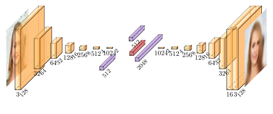
Figure 4: Encoder-Decoder Architecture used for this work

Once all the images have been encoded in $\mathbb{R}^{512}$ it is possible to use the local linear estimator of the gradient studied in this work to derive the gradient of the age with respect to the latent variable, making it possible to produce a new version of the input image that appears either older or younger as done in Figure 5. By computing a local estimate of the gradient, we are able to derive a more meaningful change when the age is not perfectly disentangled.

Figure 5: Extracting the direction of interest for aging.

Note that the quality of the image reconstruction and generation is here solely limited by the choice of the encoding and decoding model and is not related to the methods introduced in this paper, significant advances in the quality of the decoding have been made in the recent years and if a better quality and less blurry decoded output are desired we encourage the reader to replace the decoder with a PixelCNN architecture such as presented in Salimans et al. (2017). The quality of the gradient is also significantly impacted by the quality of the annotations as CACD200 is an automatically annotated and noisy dataset.

References

- Abolfathi et al. (2018) Abolfathi, B. et al. The Fourteenth Data Release of the Sloan Digital Sky Survey: First Spectroscopic Data from the Extended Baryon Oscillation Spectroscopic Survey and from the Second Phase of the Apache Point Observatory Galactic Evolution Experiment. The Astrophysical Journal Supplement Series, 235(2):42, Apr. 2018. ISSN 0067-0049. doi: 10.3847/1538-4365/aa9e8a.
- Agrawal et al. (2019) Agrawal, A., Amos, B., Barratt, S., Boyd, S., Diamond, S. and Kolter, J.Z. Differentiable convex optimization layers. In Wallach, H., Larochelle, H., Beygelzimer, A., d’Alché-Buc, F., Fox, E. and Garnett, R., editors, Advances in Neural Information Processing Systems 32, pages 9562–9574. Curran Associates, Inc., 2019.
- Bach and Jordan (2005) Bach, F.R. and Jordan, M.I. Predictive low-rank decomposition for kernel methods. In Proceedings of the 22nd International Conference on Machine Learning - ICML ’05, pages 33–40, Bonn, Germany, 2005. ACM Press. ISBN 978-1-59593-180-1. doi: 10.1145/1102351.1102356.
- Biau and Devroye (2015) Biau, G. and Devroye, L. Lectures on the Nearest Neighbor Method. Springer Series in the Data Sciences. Springer International Publishing, 2015. ISBN 978-3-319-25386-2. doi: 10.1007/978-3-319-25388-6.
- Boucheron et al. (2013) Boucheron, S., Lugosi, G. and Massart, P. Concentration Inequalities: A Nonasymptotic Theory of Independence. Oxford University Press, 2013. ISBN 978-0-19-174710-6.
- Breiman (2001) Breiman, L. Random Forests. Machine Learning, 45(1):5–32, Oct. 2001. ISSN 1573-0565. doi: 10.1023/A:1010933404324.
- Dalalyan et al. (2008) Dalalyan, A.S., Juditsky, A. and Spokoiny, V. A new algorithm for estimating the effective dimension-reduction subspace. Journal of Machine Learning Research, 9:1647–1678, Aug. 2008.
- De Brabanter et al. (2013) De Brabanter, K., De Brabanter, J., De Moor, B. and Gijbels, I. Derivative estimation with local polynomial fitting. The Journal of Machine Learning Research, 14(1):281–301, Jan. 2013. ISSN 1532-4435.
- Delecroix and Rosa (1996) Delecroix, M. and Rosa, A.C. Nonparametric estimation of a regression function and its derivatives under an ergodic hypothesis. Journal of Nonparametric Statistics, 6(4):367–382, Jan. 1996. ISSN 1048-5252. doi: 10.1080/10485259608832682.
- Detrano et al. (1989) Detrano, R. et al. International application of a new probability algorithm for the diagnosis of coronary artery disease. The American Journal of Cardiology, 64(5):304–310, Aug. 1989. ISSN 0002-9149. doi: 10.1016/0002-9149(89)90524-9.
- Devroye et al. (1996) Devroye, L., Györfi, L. and Lugosi, G. A Probabilistic Theory of Pattern Recognition. Stochastic Modelling and Applied Probability. Springer-Verlag, New York, 1996. ISBN 978-0-387-94618-4. doi: 10.1007/978-1-4612-0711-5.
- Fan (1992) Fan, J. Design-adaptive Nonparametric Regression. Journal of the American Statistical Association, 87(420):998–1004, Dec. 1992. ISSN 0162-1459, 1537-274X. doi: 10.1080/01621459.1992.10476255.
- Fan and Gijbels (1996) Fan, J. and Gijbels, I. Local Polynomial Modelling and Its Applications: Monographs on Statistics and Applied Probability 66. CRC Press, Mar. 1996. ISBN 978-0-412-98321-4.
- Gasser and Müller (1984) Gasser, T. and Müller, H.G. Estimating Regression Functions and Their Derivatives by the Kernel Method. Scandinavian Journal of Statistics, 11(3):171–185, 1984. ISSN 0303-6898.
- Giné and Guillou (2001) Giné, E. and Guillou, A. On consistency of kernel density estimators for randomly censored data: Rates holding uniformly over adaptive intervals. Annales de l’Institut Henri Poincare (B) Probability and Statistics, 37(4):503–522, July 2001. ISSN 0246-0203. doi: 10.1016/S0246-0203(01)01081-0.
- Györfi et al. (2002) Györfi, L., Kohler, M., Krzyzak, A. and Walk, H. A Distribution-Free Theory of Nonparametric Regression. Springer Series in Statistics. Springer-Verlag, New York, 2002. ISBN 978-0-387-95441-7. doi: 10.1007/b97848.
- Hastie et al. (2015) Hastie, T., Tibshirani, R. and Wainwright, M. Statistical Learning with Sparsity: The Lasso and Generalizations. Monographs on Statistics and Applied Probability. Chapman and Hall/CRC, 2015. ISBN 978-1-4987-1216-3.
- Higgins et al. (2017) Higgins, I. et al. Beta-VAE: Learning Basic Visual Concepts with a Constrained Variational Framework. ICLR, 2017.
- Hristache et al. (1998) Hristache, M., Juditsky, A. and Spokoiny, V. Direct Estimation of the Index Coefficients in a Single-index Model. Report, INRIA, May 1998.
- Hristache et al. (2001) Hristache, M., Juditsky, A., Polzehl, J. and Spokoiny, V. Structure Adaptive Approach for Dimension Reduction. Annals of Statistics, 29(6):1537–1566, Dec. 2001. ISSN 0090-5364, 2168-8966. doi: 10.1214/aos/1015345954.
- Innes et al. (2019) Innes, M. et al. A Differentiable Programming System to Bridge Machine Learning and Scientific Computing. arXiv:1907.07587 [cs], July 2019.
- Jiang (2019) Jiang, H. Non-Asymptotic Uniform Rates of Consistency for k-NN Regression. Proceedings of the AAAI Conference on Artificial Intelligence, AAAI Technical Track: Machine Learning(Vol 33 No 01: AAAI-19, IAAI-19, EAAI-20), July 2019.
- Kalivas (1997) Kalivas, J.H. Two data sets of near infrared spectra. Chemometrics and Intelligent Laboratory Systems, 37(2):255–259, June 1997. ISSN 01697439. doi: 10.1016/S0169-7439(97)00038-5.
- Kingma and Welling (2014) Kingma, D.P. and Welling, M. Auto-Encoding Variational Bayes. ICLR, 2014.
- Kpotufe (2011) Kpotufe, S. K-NN Regression Adapts to Local Intrinsic Dimension. In Shawe-Taylor, J., Zemel, R.S., Bartlett, P.L., Pereira, F. and Weinberger, K.Q., editors, Advances in Neural Information Processing Systems 24, pages 729–737. Curran Associates, Inc., 2011.
- Lecué and Mendelson (2016) Lecué, G. and Mendelson, S. Learning subgaussian classes : Upper and minimax bounds. arXiv:1305.4825 [math, stat], Sept. 2016.
- Lugosi and Mendelson (2016) Lugosi, G. and Mendelson, S. Risk minimization by median-of-means tournaments. Journal of the European Mathematical Society, 22(3), 2016.
- Massart (2007) Massart, P. Concentration Inequalities and Model Selection: Ecole d’Eté de Probabilités de Saint-Flour XXXIII - 2003. École d’Été de Probabilités de Saint-Flour. Springer-Verlag, Berlin Heidelberg, 2007. ISBN 978-3-540-48497-4. doi: 10.1007/978-3-540-48503-2.
- Mukherjee and Wu (2006) Mukherjee, S. and Wu, Q. Estimation of Gradients and Coordinate Covariation in Classification. The Journal of Machine Learning Research, 7:2481–2514, Dec. 2006. ISSN 1532-4435.
- Mukherjee and Zhou (2006) Mukherjee, S. and Zhou, D.X. Learning Coordinate Covariances via Gradients. The Journal of Machine Learning Research, 7:519–549, Dec. 2006. ISSN 1532-4435.
- Portier and Delyon (2014) Portier, F. and Delyon, B. Bootstrap Testing of the Rank of a Matrix via Least-Squared Constrained Estimation. Journal of the American Statistical Association, 109(505):160–172, Jan. 2014. ISSN 0162-1459. doi: 10.1080/01621459.2013.847841.
- Salimans et al. (2017) Salimans, T., Karpathy, A., Chen, X. and Kingma, D.P. PixelCNN++: Improving the PixelCNN with Discretized Logistic Mixture Likelihood and Other Modifications. arXiv:1701.05517 [cs, stat], Jan. 2017.
- Stone (1982) Stone, C.J. Optimal Global Rates of Convergence for Nonparametric Regression. Annals of Statistics, 10(4):1040–1053, Dec. 1982. ISSN 0090-5364, 2168-8966. doi: 10.1214/aos/1176345969.
- Street et al. (1993) Street, W.N., Wolberg, W.H. and Mangasarian, O.L. Nuclear feature extraction for breast tumor diagnosis. In Acharya, R.S. and Goldgof, D.B., editors, IS&T/SPIE’s Symposium on Electronic Imaging: Science and Technology, pages 861–870, San Jose, CA, July 1993. doi: 10.1117/12.148698.
- Talagrand (1996) Talagrand, M. New concentration inequalities in product spaces. Inventiones mathematicae, 126(3):505–563, Nov. 1996. ISSN 1432-1297. doi: 10.1007/s002220050108.
- van der vaart and Wellner (1996) van der vaart, A.W. and Wellner, J. Weak Convergence and Empirical Processes: With Applications to Statistics. Springer Series in Statistics. Springer-Verlag, New York, 1996. ISBN 978-0-387-94640-5. doi: 10.1007/978-1-4757-2545-2.
- Wang et al. (2018) Wang, Y., Du, S., Balakrishnan, S. and Singh, A. Stochastic Zeroth-order Optimization in High Dimensions. In International Conference on Artificial Intelligence and Statistics, pages 1356–1365, Mar. 2018.
- Wenocur and Dudley (1981) Wenocur, R.S. and Dudley, R.M. Some special vapnik-chervonenkis classes. Discrete Mathematics, 33(3):313–318, Jan. 1981. ISSN 0012-365X. doi: 10.1016/0012-365X(81)90274-0.
- Xia (2007) Xia, Y. A constructive approach to the estimation of dimension reduction directions. Annals of Statistics, 35(6):2654–2690, Dec. 2007. ISSN 0090-5364, 2168-8966. doi: 10.1214/009053607000000352.
- Xia et al. (2002) Xia, Y., Tong, H., Li, W.K. and Zhu, L.X. An Adaptive Estimation of Dimension Reduction Space. Journal of the Royal Statistical Society. Series B (Statistical Methodology), 64(3):363–410, 2002. ISSN 1369-7412.
- Ye and Xie (2012) Ye, G.B. and Xie, X. Learning sparse gradients for variable selection and dimension reduction. Machine Learning, 87(3):303–355, June 2012. ISSN 1573-0565. doi: 10.1007/s10994-012-5284-9.
- Zhou and Wolfe (2000) Zhou, S. and Wolfe, D.A. On Derivative Estimation In Spline Regression. Statistica Sinica, 10(1):93–108, 2000. ISSN 1017-0405.