Hyperfine structure and electric quadrupole transitions in the deuterium molecular ion

Abstract

Molecular hydrogen ions are of metrological relevance due to the possibility of precise theoretical evaluation of their spectrum and of external-field-induced shifts. In homonuclear molecular ions the electric dipole $E1$ transitions are strongly suppressed, and of primary laser spectroscopy interest is the electric quadrupole ($E2$) transition spectrum. In continuation of previous work on the H${}_{2}^{+}$ ion, we report here the results of the calculations of the hyperfine structure of the laser-induced electric quadrupole transitions between a large set of ro-vibrational states of D${}_{2}^{+}$; the inaccuracies of previous evaluations have been corrected. The effects of the laser polarization are studied in detail. We show that the electric quadrupole moment of the deuteron can in principle be determined with low fractional uncertainty $(\simeq 1\times 10^{-4})$ by comparing the results presented here with future data from precision spectroscopy of D${}_{2}^{+}$.

I Introduction

Molecular hydrogen ions (MHIs) are three-body systems that offer unique possibilities for both high precision spectroscopy and accurate theoretical evaluation of the spectrum (see, e.g., Refs. PRL2014 -science2020 and references therein). The comparison of high precision experimental and theoretical results opens room for independent tests of QED and has the potential to provide accurate values of fundamental constants. Among the most impressive achievements along this path is the recent determination of the proton-to-electron mass ratio with factional accuracy of $\sim 2\times 10^{-11}$ from rotational Alighanbari2018 and ro-vibrational science2020 precision laser spectroscopy of cooled and trapped HD⁺ ions; also confirmed were the recent adjustments of the CODATA values of the proton charge radius and the Rydberg constant. Transitions with low sensitivity to external fields are considered as promising candidates for the search for a time-variation of the mass ratios PRL2014 ; Karr2014 .

In the homonuclear MHIs H${}_{2}^{+}$, D${}_{2}^{+}$ the electric dipole transitions are strongly suppressed and the spectra are dominated by the electric quadrupole transitions, which are much weaker and have much smaller natural width. While precision laser spectroscopy of $E2$ transitions in homonuclear MHIs is still ahead in time, the theory has achieved significant progress. The first calculations of E2 spectra in the approximation of spinless particles, performed back in 1953 by Bates and Poots BatesAndPoots , were followed by works of Posen et al. Posen , Pilon and Baye Pilon2012 , and Pilon Pilon2013 of ever increasing precision. The hyperfine structure (HFS) of the $E2$-spectral lines of H${}_{2}^{+}$ was first considered in Karr2014 ; in Ref. Korobov2018 the leading effects of order $O(m_{e}\alpha^{6})$ were also included in a systematical investigation of the spectrum. The HFS of the lower excited states of D${}_{2}^{+}$ has been previously investigated in babb-psas ; Zhang2013 ; Zhang2016 . Only very few experimental studies of the HFS of D${}_{2}^{+}$ have been carried out by now v21 ; cruse .

Zhang et al. Zhang2013 and earlier Babb Bab1997 ; babb2 raised the interesting question about the possibility of determining $Q_{d}$ from the hyperfine structure of D${}_{2}^{+}$; there is now an intense discussion on its actual value. Recently, Alighanbari et al. Alighanbari-2020 determined $Q_{d}$ with fractional uncertainty $u_{r}(Q_{d})=1.5$ % from the hyperfine spectrum of a pure rotational transition of HD⁺. However, the most precise determination so far is from a comparison of experiment and theory for the neutral hydrogen molecules pavanello ; jozwiak ; komasa . Their stated uncertainties, ranging from $1\times 10^{-4}$ to $8\times 10^{-4}$, are so small that it is worthwhile to perform an independent measurement, using the molecular hydrogen ion HD⁺ or D${}_{2}^{+}$.

In the present work, we apply the approach of Korobov2018 to the deuterium ion ${\rm D_{2}^{+}}$. In Sec. II, we re-evaluate the HFS of ${\rm D_{2}^{+}}$ in the Breit-Pauli approximation by correcting inaccuracies in the preceding works. Sec. III is dedicated to the study of the laser-stimulated $E2$ transition spectrum in ${\rm D_{2}^{+}}$ with account of the HFS of the molecular levels and the polarization of the laser source. In Sec. III.4 we demonstrate that the results presented here provide the theoretical input for the composite frequency method PRL2014 ; traceless ; Alighanbari-2020 needed to determine the deuteron quadrupole moment from precision spectroscopy of D${}_{2}^{+}$ with an uncertainty comparable with the uncertainty of the latest values reported in pavanello ; puchalski . In the final Sec. IV we summarize and discuss the results.

II Hyperfine structure of deuterium molecular ion

II.1 Theoretical model

The nonrelativistic Hamiltonian of the hydrogen molecular ion ${\rm D}_{2}^{+}$ is:

$$H^{\rm NR}=\frac{\mathbf{p}_{1}^{2}}{2m_{d}}+\frac{\mathbf{p}_{2}^{2}}{2m_{d}}+\frac{\mathbf{p}_{e}^{2}}{2m_{e}}+\frac{e^{2}}{4\pi\varepsilon_{0}}\left(-\frac{1}{r_{1}}-\frac{1}{r_{2}}+\frac{1}{r_{12}}\right),$$ (1)

where $m_{d}$ and $m_{e}$ are the masses of the deuterons and the electron, $\mathbf{R}_{1}$, $\mathbf{R}_{2}$, $\mathbf{R}_{e}$ and $\mathbf{p}_{1}$, $\mathbf{p}_{2}$, $\mathbf{p}_{e}$ are the position and momentum vectors of the two deuterons and the electron in the center of mass frame, and $\mathbf{r}_{1,2}=\mathbf{R}_{e}\!-\!\mathbf{R}_{1,2}$, $\mathbf{r}_{12}=\mathbf{R}_{2}\!-\!\mathbf{R}_{1}$, $r_{1,2}=|{\bf r}_{1,2}|$, $r_{12}=|{\bf r}_{12}|$. We consider only $\Sigma_{g}$ states of D${}^{+}_{2}$; in the nonrelativistic approximation the discrete $\Sigma_{g}$ states of the hydrogen isotope molecular ions are labeled with the quantum numbers of the nuclear vibrational excitation $v$, of the total orbital momentum $L$, and of its projection on the space-fixed quantization axis $L_{z}$; the spatial parity $\lambda=\pm 1$ is constrained to $\lambda=(-1)^{L}$ and will be omitted in further notations. The nonrelativistic (Coulomb) energy levels and wave functions of D${}_{2}^{+}$ in the state $|vLL_{z}\rangle$ are denoted by $E^{{\rm(NR)}vL}$ and $\Psi^{{\rm(NR)}vLL_{z}}$, respectively.

The leading-order spin effects are described by adding to $H^{\rm NR}$ the pairwise spin interaction terms $V$ of the Breit-Pauli Hamiltonian of Ref. Bakalov2006 :

$$H=H^{\rm NR}+V,\qquad V=V_{ed_{1}}+V_{ed_{2}}+V_{dd},$$ (2)

where $d_{1}$ and $d_{2}$ denote the two deuterium nuclei of D${}_{2}^{+}$. We remind the explicit form of the spin interaction operators; to comply with the established traditions we shall use atomic units $\hbar=e=4\pi\varepsilon_{0}=1$ in the remainder of Sect. II.1.

$$\begin{array}[]{@{}l}\displaystyle V_{ed_{1}}=\alpha^{2}\biggl{[}-\frac{4\pi}{3}\,\mu_{e}\mu_{d}\,\frac{m_{e}}{m_{p}}\,\delta({\bf r}_{1})\,({\bf s}_{e}\cdot{\bf I}_{1})+\left(\mu_{e}-\frac{1}{2}\right)\frac{1}{r_{1}^{3}}({\bf r}_{1}\times{\bf p}_{e})\cdot{\bf s}_{e}-\mu_{e}\frac{m_{e}}{m_{d}}\frac{1}{r_{1}^{3}}({\bf r}_{1}\times{\bf p}_{1})\cdot{\bf s}_{e}\\[8.53581pt] \displaystyle\hskip 34.1433pt-\frac{m_{e}}{2m_{d}}\left(\mu_{d}\frac{m_{e}}{m_{p}}-\frac{m_{e}}{m_{d}}\right)\frac{1}{r_{1}^{3}}({\bf r}_{1}\times{\bf p}_{1})\cdot{\bf I}_{1}+\mu_{d}\frac{m_{e}}{2m_{p}}\frac{1}{r_{1}^{3}}({\bf r}_{1}\times{\bf p}_{e})\cdot{\bf I}_{1}\biggr{]}\\[8.53581pt] \displaystyle\hskip 34.1433pt+\alpha^{2}\left[\mu_{e}\mu_{d}\,\frac{m_{e}}{2m_{p}}\frac{r_{1}^{2}({\bf s}_{e}\cdot{\bf I}_{1})-3({\bf r}_{1}\cdot{\bf s}_{e})({\bf r}_{1}\cdot{\bf I}_{1})}{r_{1}^{5}}\right]+\frac{Q_{d}}{2a_{0}^{2}}\,\frac{r_{1}^{2}{\bf I}_{1}^{2}-3({\bf r}_{1}\cdot{\bf I}_{1})^{2}}{r_{1}^{5}}\,,\end{array}$$ (3)

$$V_{ed_{2}}=V_{ed_{1}}(\mathbf{r}_{1}\to\mathbf{r}_{2},\mathbf{p}_{1}\to\mathbf{p}_{2},\mathbf{I}_{1}\to\mathbf{I}_{2}),$$ (4)

$$\begin{array}[]{@{}l}\displaystyle V_{dd}=\alpha^{2}\biggl{[}-\frac{2\pi}{3}\mu_{d}^{2}\,\frac{m_{e}^{2}}{m_{p}^{2}}\,\delta({\bf r}_{12})\,({\bf I}_{1}\cdot{\bf I}_{2})+\frac{\mu_{d}m_{e}^{2}}{2m_{p}m_{d}}\left(\frac{1}{r_{12}^{3}}({\bf r}_{12}\times{\bf p}_{1})\cdot{\bf I}_{2}-\frac{1}{r_{12}^{3}}({\bf r}_{12}\times{\bf p}_{2})\cdot{\bf I}_{1}\right)\\[8.53581pt] \displaystyle\hskip 34.1433pt+\frac{m_{e}}{2m_{d}}\left(\mu_{d}\frac{m_{e}}{m_{p}}-\frac{m_{e}}{m_{d}}\right)\left(\frac{1}{r_{12}^{3}}({\bf r}_{12}\times{\bf p}_{1})\cdot{\bf I}_{1}-\frac{1}{r_{12}^{3}}({\bf r}_{12}\times{\bf p}_{2})\cdot{\bf I}_{2}\right)\biggr{]}\\[9.95845pt] \displaystyle\hskip 34.1433pt+\alpha^{2}\left[\mu_{d}^{2}\,\frac{m_{e}^{2}}{4m_{p}^{2}}\frac{r_{12}^{2}({\bf I}_{1}\cdot{\bf I}_{2})-3({\bf r}_{12}\cdot{\bf I}_{1})({\bf r}_{12}\cdot{\bf I}_{2})}{r_{12}^{5}}\right]-\frac{Q_{d}}{2a_{0}^{2}}\sum\limits_{i=1,2}\frac{r_{12}^{2}{\bf I}_{i}^{2}-3({\bf r}_{12}\cdot{\bf I}_{i})^{2}}{r_{12}^{5}}\,.\end{array}$$ (5)

Here $\mathbf{I}_{1,2}$ and $\mathbf{s}_{e}$ are the spin operators of the two deuterons and of the electron, respectively, and proper symmetrization of the terms containing non-commuting operators is assumed; $\mu_{e}$ is the magnetic dipole moment of the electron in units $\mu_{0}=e\hbar/2m_{e}$ (Bohr magneton), $\mu_{d}$ is the magnetic dipole moment of the deuteron in units $\mu_{N}=e\hbar/2m_{p}$ (nuclear magneton), $a_{0}$ is the Bohr radius, and $Q_{d}$ is the electric quadrupole moment of the deuteron. The same spin-interaction Hamiltonian was used in Zhang2013 .

The spin interactions split the degenerate nonrelativistic energy levels $E^{{\rm(NR)}vL}$ into a manifold of hyperfine levels that are distinguished with additional quantum numbers (QNs) describing their “spin composition”. As evidenced in subsection II.3, the appropriate angular momentum coupling scheme for D${}_{2}^{+}$ is

$$\mathbf{I}=\mathbf{I}_{1}+\mathbf{I}_{2},\qquad\mathbf{F}=\mathbf{I}+\mathbf{s}_{e},\qquad\mathbf{J}=\mathbf{L}+\mathbf{F}.$$

Accordingly, the hyperfine states are labelled with the exact QNs of the total angular momentum $J$ and its projection $J_{z}$, and the approximate QNs $I$, $F$ and $L$. Similar to Refs. Bakalov2006 ; Zhang2013 ; Korobov2018 , in first order of perturbation theory the hyperfine levels $E^{(vL)IFJJ_{z}}$ may be put in the form $E^{(vL)IFJJ_{z}}=E^{{\rm(NR)}vL}+\Delta E^{(vL)IFJJ_{z}}$, where the corrections $\Delta E^{(vL)IFJJ_{z}}$, also referred to as ’hyperfine energies’ or ’hyperfine shifts’, are the eigenvalues of the effective spin interaction Hamiltonian $H^{\rm eff}$. (Of course, in absence of external fields the energies are degenerate in $J_{z}$). Instead of the above, however, we shall use the more general form

$$E^{(vL)IFJJ_{z}}=E^{{\rm(diag)}vL}+\Delta E^{(vL)IFJJ_{z}},$$ (6)

where $E^{{\rm(diag)}vL}$ also includes the relativistic, QED, etc. spin-independent corrections to the non-relativistic energy levels $E^{{\rm(NR)}vL}$. Since the evaluation of $\Delta E^{(vL)IFJ}$ is the point where our results disagree to some extent with the results of Refs. Zhang2013 ; Zhang2016 , we give more details of the calculations.

II.2 Effective spin Hamiltonian

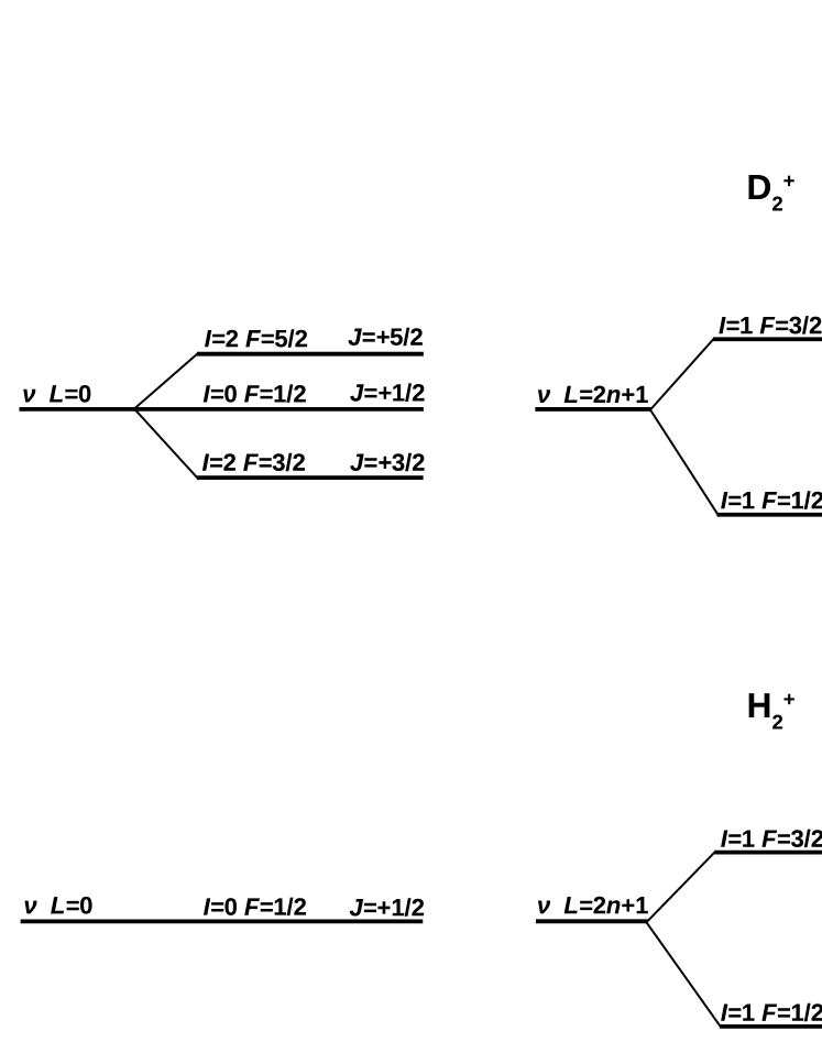
Figure 1: Comparison of the hyperfine structure of the molecular ions D${}_{2}^{+}$ and H${}_{2}^{+}$, for even $L=2n,n=1,2,\ldots$ and odd $L=2n+1,n=0,1,\ldots$ values of $L$ and for $L\!=\!0$. For $1\leq L\leq 2$ the states marked with dashed lines do not exist (see Tables 2,3). For $L\!=\!0$ the HFS of D${}_{2}^{+}$ consists of only three states; similar to H${}_{2}^{+}$ the one with $I\!=\!0$ has no hyperfine shift.

We associate with the spin of the deuteron $d_{1}$ the $(2I_{1}+1)$-dimensional space of the irreducible representation $(I_{1})$ of $su(2)$ with basis vectors $|I_{1}I_{1z}\rangle,I_{1z}=-I_{1},\ldots,I_{1}$, satisfying

$$\hat{\mathbf{I}}_{1}^{2}|I_{1}I_{1z}\rangle=I_{1}(I_{1}\!+\!1)|I_{1}I_{1z}\rangle,\qquad\hat{I}_{1z}|I_{1}I_{1z}\rangle=I_{1z}|I_{1}I_{1z}\rangle.$$

Similarly, we define the sets $|I_{2}I_{2z}\rangle$, $|s_{e}s_{ez}\rangle$, and $|LL_{z}\rangle$. The basis set $|IFF_{z}\rangle$ in the resulting space of the spin variables of all D${}_{2}^{+}$ constituents is taken in the form:

$$|IFF_{z}\rangle=\sum\limits_{I_{1z}I_{2z}s_{ez}I_{z}}C_{I_{1}I_{1z},I_{2}I_{2z}}^{II_{z}}C_{II_{z},s_{e}s_{ez}}^{FF_{z}}|I_{1}I_{1z}\rangle|I_{2}I_{2z}\rangle|s_{e}s_{ez}\rangle,$$ (7)

here $C_{l_{1}m_{1},l_{2}m_{2}}^{LM}=\left\langle l_{1}l_{2}m_{1}m_{2}|LM\right\rangle$ are Clebsch-Gordan coefficients. Thus, the basis set in the hyperfine manifold of the $(vL)$ state of D${}_{2}^{+}$ consists of the functions

$$\Psi_{0}^{(vL)IFJJ_{z}}=\sum\limits_{L_{z}F_{z}}C_{LL_{z},FF_{z}}^{JJ_{z}}\,\Psi^{{\rm(NR)}vLL_{z}}\,|IFF_{z}\rangle.$$ (8)

We also define a basis set depending on the angular part only, which will be referred to as ”pure” states,

$$|LIFJJ_{z}\rangle=\sum\limits_{L_{z},F_{z}}C_{LL_{z},FF_{z}}^{JJ_{z}}|LL_{z}\rangle|IFF_{z}\rangle.$$ (9)

The effective spin Hamiltonian $H^{\rm eff}$ is a matrix operator acting on the finite-dimensional space spanned by the vectors $|LIFJJ_{z}\rangle$, such that

$$H^{{\rm eff}(vL)J}_{I^{\prime}F^{\prime},IF}\equiv\langle LI^{\prime}F^{\prime}JJ_{z}|H^{\rm eff}|LIFJJ_{z}\rangle=\langle\Psi_{0}^{(vL)I^{\prime}F^{\prime}JJ_{z}}|V|\Psi_{0}^{(vL)IFJJ_{z}}\rangle.$$ (10)

In absence of external fields the matrix of $H^{{\rm eff}(vL)J}_{I^{\prime}F^{\prime},IF}$ is independent of $J_{z}$. For the deuterium molecular ion $H^{\rm eff}$ has the form

$$\begin{array}[]{@{}l}\displaystyle H^{\rm eff}=E_{1}(\mathbf{L}\cdot\mathbf{s}_{e})+E_{2}(\mathbf{L}\cdot\mathbf{I})+E_{3}(\mathbf{I}\cdot\mathbf{s}_{e})\\[5.69054pt] \displaystyle\hskip 31.29802pt+E_{4}\bigl{(}2\mathbf{L}^{2}(\mathbf{I}\cdot\mathbf{s}_{e})-3\left((\mathbf{L}\cdot\mathbf{I})(\mathbf{L}\cdot\mathbf{s}_{e})+(\mathbf{L}\cdot\mathbf{s}_{e})(\mathbf{L}\cdot\mathbf{I})\right)\bigr{)}\\[7.11317pt] \displaystyle\hskip 31.29802pt+E_{5}\big{(}2\mathbf{L}^{2}(\mathbf{I}_{1}\cdot\mathbf{I}_{2})-3\left((\mathbf{L}\cdot\mathbf{I}_{1})(\mathbf{L}\cdot\mathbf{I}_{2})+(\mathbf{L}\cdot\mathbf{I}_{2})(\mathbf{L}\cdot\mathbf{I}_{1})\right)\big{)}\\[1.42262pt] \displaystyle\hskip 31.29802pt+E_{6}\left[{\bf L}^{2}{\bf I}_{1}^{2}-\frac{3}{2}({\bf L}\cdot{\bf I}_{1})-3({\bf L}\cdot{\bf I}_{1})^{2}+{\bf L}^{2}{\bf I}_{2}^{2}-\frac{3}{2}({\bf L}\cdot{\bf I}_{2})-3({\bf L}\cdot{\bf I}_{2})^{2}\right].\end{array}$$ (11)

Compared to the effective spin Hamiltonian for H${}^{+}_{2}$ of Ref. Korobov2018 , $H^{\rm eff}$ of Eq. (11) includes one additional term (with $E_{6}$, last line) that describes the effects due to the electric quadrupole moment of the nuclei and arises when averaging the last term in Eqs. (3-5). The first four terms in Eq. (11) coincide with the first four terms in the effective Hamiltonian of Refs. Zhang2013 ; Zhang2016 , defined in Eqs. (12)-(15) of the former, with account of the correspondence between the notations used: $E_{1}=c_{e}$, $E_{2}=c_{I}$, $E_{3}=b_{F}$, $E_{4}=d_{1}/(3(2L-1)(2L+3))$. The last two terms involving $E_{5}$ and $E_{6}$, however, do not. The disagreement appears in the terms related to the tensor interaction of the deuterons in the last lines of Eqs. (3) and (5). The explicit expressions for $E_{4}$–$E_{6}$ are:

$$\begin{array}[]{@{}l}\displaystyle E_{4}=\alpha^{2}\mu_{e}\mu_{d}\frac{m_{e}}{2m_{p}}\left[\frac{\langle vL\|r_{1}^{-5}(\mathbf{r}_{1}^{2}\delta_{i\!j}-3r_{1i}r_{1j})\|vL\rangle}{\langle L\|2\mathbf{L}^{2}\delta_{i\!j}-3(L_{i}L_{j}\!+\!L_{j}L_{i})\|L\rangle}+(1\to 2)\right],\\[8.53581pt] \displaystyle E_{5}=\alpha^{2}\left(\frac{\mu_{d}m_{e}}{2m_{p}}\right)^{2}\frac{\langle vL\|r_{12}^{-5}(\delta_{i\!j}\mathbf{r}_{12}^{2}-3r_{12i}r_{12j})\|vL\rangle}{\langle L\|2\mathbf{L}^{2}\delta_{i\!j}-3(L_{i}L_{j}\!+\!L_{j}L_{i})\|L\rangle}\,,\\[8.53581pt] \displaystyle E_{6}=Q_{d}\bar{E}_{6},\ \bar{E}_{6}=\frac{1}{2}\left[\frac{\langle vL\|r_{1}^{-5}(\delta_{i\!j}\mathbf{r}_{1}^{2}-3r_{i}r_{j})\|vL\rangle-\langle vL\|r_{12}^{-5}(\delta_{i\!j}\mathbf{r}_{12}^{2}-3r_{12i}r_{12j})\|vL\rangle}{\langle L\|\mathbf{L}^{2}\delta_{i\!j}-(3/2)(L_{i}L_{j}\!+\!L_{j}L_{i})\|L\rangle}+(1\to 2)\right],\end{array}$$ (12)

where $\langle v^{\prime}L^{\prime}\|\ldots\|vL\rangle$ denote reduced matrix elements in the basis of nonrelativistic wave functions $\psi^{{\rm(NR)}vLL_{z}}$, while

$$\langle L\|2\mathbf{L}^{2}\delta_{ij}-3(L_{i}L_{j}\!+\!L_{j}L_{i})\|L\rangle=-2\sqrt{L(L\!+\!1)}\sqrt{(2L\!-\!1)(2L\!+\!1)(2L\!+\!3)}.$$

is a reduced matrix element in the basis of the representation $(L)$ of $su(2)$ (see Eqs. (7),(9)). The point is that the tensor terms in $H^{\rm eff}$ have non-zero matrix elements between ”pure” states states with even $L$ and different values of the total nuclear spin $I=0$ and $I^{\prime}=2$:

$$\langle\nu LIFJ\|H^{\rm eff}\|\nu LI^{\prime}F^{\prime}J\rangle=10\sqrt{3}(-1)^{J+2F+L+1/2}$$ (13)

$$\times\sqrt{(2F+1)(2F^{\prime}+1)}L(L+1)(2L+1)\left\{\begin{matrix}F^{\prime}&\!F\!&2\\ L&\!L\!&J\end{matrix}\right\}\left\{\begin{matrix}1&\!1\!&2\\ L&\!L\!&L\end{matrix}\right\}\left\{\begin{matrix}I&\!1/2\!&F\\ F^{\prime}&\!2\!&I^{\prime}\end{matrix}\right\}\left(E_{5}-E_{6}\right),$$

while the effective Hamiltonian of Refs. Zhang2013 ; Zhang2016 is diagonal in $\mathbf{I}$. Neglecting the coupling of pure states with different $I$ affects the values of the hyperfine shifts at the kHz level, as illustrated in Table 4 of Section II.3.

In first order of perturbation theory the wave functions of D${}_{2}^{+}$ are linear combinations of the basis set (8):

$$\Psi^{(vL)IFJJ_{z}}=\sum\limits_{I^{\prime}F^{\prime}}\beta^{(vL)IFJ}_{I^{\prime}F^{\prime}}\Psi^{(vL)I^{\prime}F^{\prime}JJ_{z}}_{0},$$ (14)

where the constant amplitudes $\beta^{(vL)IFJ}_{I^{\prime}F^{\prime}}$ and the hyperfine shifts $\Delta E^{(vL)IFJ}$ are the eigenvectors and eigenvalues of the matrix of $H^{\rm eff}$ in the basis of pure states (9):

$$\sum\limits_{I^{\prime\prime}F^{\prime\prime}}H^{{\rm eff}(vL)J}_{I^{\prime}F^{\prime},I^{\prime\prime}F^{\prime\prime}}\ \beta^{(vL)IFJ}_{I^{\prime\prime}F^{\prime\prime}}=\Delta E^{(vL)IFJ}\beta^{(vL)IFJ}_{I^{\prime}F^{\prime}}.$$ (15)

Similar to H${}_{2}^{+}$, symmetry with respect to exchange of the identical nuclei imposes restrictions on the allowed values of $I$ in the summation in Eqs. (14), (15); for $\Sigma_{g}$ states, in particular, $I$ must satisfy $(-1)^{L+I}=1$. As a result, in H${}^{+}_{2}$, in first order of perturbation theory, $I$ turns out to be an exact quantum number Korobov2018 . This is not the case for D${}_{2}^{+}$, however, where both values $I=0$ and $I=2$ are allowed for even values of $L$, although their mixing is weak. Still, a few of the hyperfine states of D${}_{2}^{+}$ are “pure states” with no mixing and all quantum numbers exact; these are the states with $I=1$, $F=3/2$, $J=L\pm F$ (for odd $L$), the states with $I=2$, $F=5/2$, $J=L\pm F$ (for even $L\geq 2$), as well as the states with $L=0$ and either $I=0,J=F=1/2$ or $I=2,J=F=I\pm 1/2$. The “stretched” states with $F=I+1/2$, $J=L+F$, and $J_{z}=\pm J$, of significant experimental interest because their Zeeman shift is strictly linear in the magnetic field in first order of perturbation theory jpb44 , are a sub-class of the “pure” states listed above. The hyperfine energy $\Delta E\equiv\Delta E^{(vL)IFJ}$ of the “pure” states is simply expressed in terms of the coefficients of the effective spin Hamiltonian as follows:

$$\Delta E^{(vL)IFJ}=\frac{1}{2}\big{(}E_{3}+L(E_{1}+2E_{2}+(2L-1)(E_{6}-2E_{4}-2E_{5}))\big{)},\ \text{for}\ I=1,F=3/2,J=L+F,\ \text{odd}\ L;$$

$$\Delta E^{(vL)IFJ}=\frac{1}{2}\big{(}E_{3}-(L+1)(E_{1}+2E_{2}+(2L+3)(E_{6}-2E_{4}-2E_{5}))\big{)},\ \text{for}\ I=1,F=3/2,J=L-F,\ \text{odd}\ L\geq 3;$$

$$\Delta E^{(vL)IFJ}=E_{3}+L(E_{1}/2+2E_{2}-(2L-1)(2E_{4}+2E_{5}+E_{6})),\ \text{for}\ I=2,F=5/2,J=L+F,\ \text{even}\ L\geq 2;$$

$$\Delta E^{(vL)IFJ}=E_{3}-(L+1)(E_{1}/2+2E_{2}+(2L+3)(2E_{4}+2E_{5}+E_{6})),\ \text{for}\ I=2,F=5/2,J=L-F,\ \text{even}\ L\geq 4;$$

$$\Delta E^{(v0)0FJ}=0\ \text{for}\ J=F=1/2,$$

$$\Delta E^{(v0)2FJ}=-3E_{3}/2\ \text{for}\ J=F=3/2,$$

$$\Delta E^{(v0)2FJ}=E_{3}\ \text{for}\ J=F=5/2.$$

II.3 Numerical results

The numerical results of the present work were obtained using the non-relativistic wave functions $\Psi^{{\rm(NR)}vLL_{z}}$ of D${}^{+}_{2}$, calculated with high numerical precision in the variational approach of Ref. KorobovVarMethod . Throughout the calculations the CODATA18 values nist of fundamental constants were used for $m_{d}/m_{p}$, $\mu_{e}$, and $\mu_{d}$, while $Q_{d}=0.285783\text{ fm}^{2}$ was taken from pavanello . Table 1 gives the values of $E_{n},n=1,\ldots,6$ for the lower ro-vibrational states of D${}_{2}^{+}$; the values for all ro-vibrational states $(vL)$ with $v\leq 10$ and $L\leq 4$ can be found in the electronic supplement suppl . We list the numerical values of $E_{n},n=1,\ldots,6$ with 6 significant digits to avoid rounding errors in further calculations, but one should keep in mind that the contribution from QED and relativistic effects of order $O(m_{e}\alpha^{6})$ and higher is not accounted for by the Breit-Pauli Hamiltonian. We denote by $u(E_{n})$ and $u_{r}(E_{n})$ the absolute and fractional uncertainties of $E_{n}$; $u_{r}(E_{n}),n\leq 5$ are therefore estimated to be order $O(\alpha^{2})\sim 0.5\times 10^{-4}$ (for $u_{r}(E_{6})$ see Eq. (16) below). The numerical uncertainty stemming from numerical integration of the non-relativistic wave functions $\Psi^{{\rm(NR)}vLL_{z}}$ is smaller. Also smaller is the contribution to $u_{r}(E_{n})$ from the uncertainty in the values of the physical constants in the Breit-Pauli Hamiltonian (3-5), with the important exception of $E_{6}$, for which the uncertainty $u(Q_{d})$ of the electric quadrupole moment contributes substantially. Indeed, from Eq. (12) we obtain

$$u_{r}(E_{6})=\frac{u(E_{6})}{E_{6}}=\sqrt{u_{r}^{2}(Q_{d})+u_{r}^{2}(\bar{E}_{6})}\text{\ with\ }u_{r}(\bar{E}_{6})\sim u_{r}(E_{n})\sim O(\alpha^{2}),n=1,...,5.$$ (16)

The uncertainty of $Q_{d}$ arises from uncertainties of both the experimental data and the underlying molecular theory (when $Q_{d}$ is determined by molecular spectroscopy). The relation between $u_{r}(Q_{d})$ and the theoretical uncertainties in the case of D${}_{2}^{+}$ spectroscopy is treated in detail in Sec. III.4.

$v$	$L$	$E_{1}/h$	$E_{2}/h$	$E_{3}/h$	$E_{4}/h$	$E_{5}/h$	$E_{6}/h$
0	0			$142.533$
1	0			$139.837$
2	0			$137.286$
3	0			$134.873$
4	0			$132.593$
0	1	$21.4599$	$-3.21518[-3]$	$142.448$	$1.32980$	$-4.71443[-4]$	$5.67068[-3]$
1	1	$20.5231$	$-3.12947[-3]$	$139.756$	$1.26978$	$-4.57403[-4]$	$5.66924[-3]$
2	1	$19.6183$	$-3.04185[-3]$	$137.209$	$1.21191$	$-4.43279[-4]$	$5.64719[-3]$
3	1	$18.7423$	$-2.95244[-3]$	$134.799$	$1.15600$	$-4.29061[-4]$	$5.60575[-3]$
4	1	$17.8923$	$-2.86128[-3]$	$132.522$	$1.10187$	$-4.14738[-4]$	$5.54600[-3]$
0	2	$21.3955$	$-3.20207[-3]$	$142.278$	$3.15886[-1]$	$-1.11799[-4]$	$1.34038[-3]$
1	2	$20.4612$	$-3.11645[-3]$	$139.594$	$3.01623[-1]$	$-1.08462[-4]$	$1.34003[-3]$
2	2	$19.5586$	$-3.02901[-3]$	$137.054$	$2.87871[-1]$	$-1.05106[-4]$	$1.33480[-3]$
3	2	$18.6847$	$-2.93977[-3]$	$134.652$	$2.74583[-1]$	$-1.01728[-4]$	$1.32498[-3]$
4	2	$17.8368$	$-2.84875[-3]$	$132.382$	$2.61720[-1]$	$-9.83254[-5]$	$1.31082[-3]$
0	3	$21.2995$	$-3.18256[-3]$	$142.025$	$1.46902[-1]$	$-5.18607[-5]$	$6.18729[-4]$
1	3	$20.3688$	$-3.09714[-3]$	$139.353$	$1.40266[-1]$	$-5.03083[-5]$	$6.18561[-4]$
2	3	$19.4696$	$-3.00991[-3]$	$136.824$	$1.33867[-1]$	$-4.87468[-5]$	$6.16135[-4]$
3	3	$18.5989$	$-2.92092[-3]$	$134.432$	$1.27684[-1]$	$-4.71753[-5]$	$6.11585[-4]$
4	3	$17.7541$	$-2.83015[-3]$	$132.173$	$1.21697[-1]$	$-4.55926[-5]$	$6.05027[-4]$
0	4	$21.1727$	$-3.15685[-3]$	$141.691$	$8.54566[-2]$	$-3.00678[-5]$	$3.56385[-4]$
1	4	$20.2467$	$-3.07169[-3]$	$139.033$	$8.15938[-2]$	$-2.91641[-5]$	$3.56285[-4]$
2	4	$19.3519$	$-2.98476[-3]$	$136.519$	$7.78684[-2]$	$-2.82552[-5]$	$3.54880[-4]$
3	4	$18.4855$	$-2.89608[-3]$	$134.142$	$7.42682[-2]$	$-2.73407[-5]$	$3.52246[-4]$
4	4	$17.6446$	$-2.80567[-3]$	$131.896$	$7.07820[-2]$	$-2.64197[-5]$	$3.48452[-4]$

Table 1: Coefficients of the effective spin interaction Hamiltonian of Eq. (11) for the lower ro-vibrational states of D${}^{+}_{2}$ with $L\leq 4$, $v\leq 10$, in MHz. The number in brackets denote powers of ten: $a[b]=a\times 10^{b}$. Note that for $L=0$ all coefficients but $E_{3}$ are zero.

The hyperfine energies $\Delta E^{(vL)IFJ}$ and the amplitudes $\beta^{(vL)IFJ}_{I^{\prime}F^{\prime}}$ of the states from the hyperfine structure of the lower excited states, calculated using Eqs. (10), (11), and (15), are given in Tables 2 and 3. The results for the higher excited states with $v$ up to 10 or $L$ up to 4 are available in the electronic supplement suppl . The theoretical uncertainties $u(\Delta E^{(vL)IFJ})$ of the hyperfine energies $\Delta E^{(vL)IFJ}$ were estimated in the assumption that the uncertainties of the coefficients $E_{n}$ are uncorrelated, and are given by

$$u(\Delta E^{(vL)IFJ})=\sqrt{\sum_{n}\left(u_{r}(E_{n})\ \Gamma^{(vL)IFJ}_{n}\right)^{2}}\text{\ with\ }\Gamma^{(vL)IFJ}_{n}=E_{n}\frac{\partial\Delta E^{(vL)IFJ}}{\partial E_{n}}.$$ (17)

For states with the smallest shifts ($\simeq 20\,$ MHz, in which the influence of the coefficient $E_{3}$ is comparatively small), the uncertainties $u(\Delta E^{(vL)IFJ})$ are of order 1 kHz, while for hyperfine states with shifts of the order of 100 MHz and above the theoretical uncertainty may reach $\sim 10$ kHz.

In the lower ro-vibrational states of D${}_{2}^{+}$ the dominating term of the Breit-Pauli Hamiltonian (3-5) is the contact spin-spin interaction between the electron and the nuclei; this can be recognized by comparing the value of $E_{3}$ with the other coefficients of the effective spin Hamiltonian $H^{\rm eff}$ (11), given in Table 1 and the electronic supplement suppl . The contribution to $\Delta E^{(vL)IFJ}$ of the $E_{3}$-term alone is $(E_{3}/2)(F(F+1)-I(I+1)-3/4)$; similar to H${}_{2}^{+}$ it qualitatively determines the shape of the hyperfine level structure (see Fig. 1), and for $L=0$ this is the only contribution to the hyperfine energy. The typical separation between hyperfine levels of D${}_{2}^{+}$ with different values of $F$ or $I$ is of the order of $E_{3}\sim 10^{2}$ MHz. It is significantly smaller than the GHz separation in H${}_{2}^{+}$ or HD⁺ because of the smaller magnetic dipole moment of the deuteron $\mu_{d}$ as compared with $\mu_{p}$. For all three molecular ions the separation between states with $\Delta J=\pm 1$ is of the order of 10 MHz. The off-diagonal elements of the matrix $\beta^{IFJ}_{I^{\prime}F^{\prime}}$ (see Eq. (14)) are small, i.e. the mixing of states with different values of $I$ or $F$ is weak. This justifies our choice of the angular momentum coupling scheme, and allows to use in estimates of the characteristics of D${}_{2}^{+}$ (except for the hyperfine shifts) the approximation of pure states $\beta^{IFJ}_{I^{\prime}F^{\prime}}=\delta_{F^{\prime}F}\delta_{I^{\prime}I}$.

$I$	$F$	$J$	$\Delta E^{\rm hfs}/h$	$\beta^{IFJ}_{1,1/2}$	$\beta^{IFJ}_{1,3/2}$	$\left(d\Delta E^{\rm hfs}/dQ_{d}\right)/h$
$v=0$, $L=1$
1	1/2	3/2	-146.999(8)	0.99776	-0.06688	2.78
1	1/2	1/2	-136.493(7)	0.99673	-0.08075	-10.97
1	3/2	1/2	47.916(4)	0.08075	0.99673	60.58
1	3/2	3/2	70.351(4)	0.06688	0.99776	-42.47
1	3/2	5/2	80.624(4)	0.00000	1.00000	9.92
$v=1$, $L=1$
1	1/2	3/2	-144.085(7)	0.99787	-0.06524	2.72
1	1/2	1/2	-134.026(7)	0.99692	-0.07838	-10.66
1	3/2	1/2	47.564(4)	0.07838	0.99692	60.25
1	3/2	3/2	69.012(4)	0.06524	0.99787	-42.39
1	3/2	5/2	78.870(4)	0.00000	1.00000	9.92
$v=2$, $L=1$
1	1/2	3/2	-141.325(7)	0.99798	-0.06356	2.64
1	1/2	1/2	-131.698(7)	0.99711	-0.07598	-10.30
1	3/2	1/2	47.251(4)	0.07598	0.99711	59,70
1	3/2	3/2	67.746(4)	0.06356	0.99798	-42.16
1	3/2	5/2	77.202(4)	0.00000	1.00000	9.88
$v=0$, $L=3$
1	1/2	7/2	-157.925(7)	0.98895	-0.14826	7.53
1	1/2	5/2	-134.446(7)	0.98227	-0.18749	-16.39
1	3/2	3/2	23.151(4)	0.00000	1.00000	3.87
1	3/2	5/2	54.118(3)	0.18749	0.98227	6.65
1	3/2	7/2	80.653(4)	0.14826	0.98895	-40.01
1	3/2	9/2	100.754(4)	0.00000	1.00000	16.24
$v=1$, $L=3$
1	1/2	7/2	-154.445(7)	0.98944	-0.14497	7.38
1	1/2	5/2	-131.922(7)	0.98324	-0.18230	-15.94
1	3/2	3/2	23.914(4)	0.00000	1.00000	38.96
1	3/2	5/2	53.336(3)	0.18230	0.98324	6.20
1	3/2	7/2	78.775(4)	0.14497	0.98944	-39.85
1	3/2	9/2	98.122(4)	0.00000	1.00000	16.23
$v=2$, $L=3$
1	1/2	7/2	-151.139(7)	0.98992	-0.14161	7.20
1	1/2	5/2	-129.544(7)	0.98421	-0.17702	-15.42
1	3/2	3/2	24.678(4)	0.00000	1.00000	38.81
1	3/2	5/2	52.614(3)	0.17702	0.98421	5.72
1	3/2	7/2	76.992(3)	0.14161	0.98992	-39.54
1	3/2	9/2	95.605(4)	0.00000	1.00000	16.17

Table 2: Hyperfine structure of the lower ro-vibrational states for odd values $L=1,3$. Listed are: the quantum numbers $J$, $I$, and $F$, the hyperfine energy $\Delta E^{\rm hfs}=\Delta E^{(vL)IFJ}/h$ (in MHz), the amplitudes $\beta^{(vL)IFJ}_{I^{\prime}F^{\prime}}$ of the spin wave function, and the derivative $h^{-1}\,d\Delta E^{\rm hfs}/dQ_{d}$ (in kHz fm${}^{-2}).$ The pure states are typed in boldface.

$I$	$F$	$J$	$\Delta E^{\rm hfs}/h$	$\beta^{IFJ}_{0,1/2}$	$\beta^{IFJ}_{2,3/2}$	$\beta^{IFJ}_{2,5/2}$	$\left(d\Delta E^{\rm hfs}/dQ_{d}\right)/h$
$v=0$, $L=0$
2	3/2	3/2	-213.800(11)	0.00000	1.00000	0.00000	0.00000
0	1/2	1/2	0.000(8)	1.00000	0.00000	0.00000	0.00000
2	5/2	5/2	142.533(8)	0.00000	0.00000	1.00000	0.00000
$v=1$, $L=0$
2	3/2	3/2	-209.756(11)	0.00000	1.00000	0.00000	0.00000
0	1/2	1/2	0.000(0)	1.00000	0.00000	0.00000	0.00000
2	5/2	5/2	139.837(7)	0.00000	0.00000	1.00000	0.00000
$v=0$, $L=2$
2	3/2	7/2	-226.255(11)	0.00000	0.99852	-0.05446	-22.25
2	3/2	5/2	-216.433(11)	0.00004	0.99669	-0.08128	51.39
2	3/2	3/2	-202.716(11)	-0.00012	0.99664	-0.08194	5.06
2	3/2	1/2	-190.986(11)	0.00000	0.99863	-0.05238	-66.45
0	1/2	3/2	-32.093(2)	1.00000	0.00012	0.00006	0.01
0	1/2	5/2	21.395(1)	1.00000	-0.00002	0.00019	-0.02
2	5/2	1/2	102.515(8)	0.00000	0.05238	0.99863	-81.29
2	5/2	3/2	117.107(7)	-0.00007	0.08194	0.99664	-33.21
2	5/2	5/2	135.572(7)	-0.00019	0.08128	0.99669	26.03
2	5/2	7/2	151.994(7)	0.00000	0.05446	0.99852	50.39
2	5/2	9/2	159.864(8)	0.00000	0.00000	1.00000	-28.14
$v=1$, $L=2$
2	3/2	7/2	-221.646(11)	0.00000	0.99858	-0.05318	-22.19
2	3/2	5/2	-212.213(11)	0.00004	0.99686	-0.07921	51.32
2	3/2	3/2	-199.097(11)	-0.00012	0.99682	-0.07963	4.92
2	3/2	1/2	-187.921(11)	0.00000	0.99871	-0.05076	-66.51
0	1/2	3/2	-30.692(2)	1.00000	0.00013	0.00007	0.01
0	1/2	5/2	20.461(1)	1.00000	-0.00002	0.00019	-0.02
2	5/2	1/2	101.558(8)	0.00000	0.05076	0.99871	-81.19
2	5/2	3/2	115.469(7)	-0.00008	0.07963	0.99682	-33.07
2	5/2	5/2	133.118(7)	-0.00019	0.07921	0.99686	26.07
2	5/2	7/2	148.851(7)	0.00000	0.05318	0.99858	50.33
2	5/2	9/2	156.416(7)	0.00000	0.00000	1.00000	-28.13
$v=2$, $L=2$
2	3/2	7/2	-217.273(11)	0.00000	0.99865	-0.05189	-22.05
2	3/2	5/2	-208.218(11)	0.00004	0.99702	-0.07710	51.07
2	3/2	3/2	-195.684(11)	-0.00012	0.99701	-0.07728	4.76
2	3/2	1/2	-185.041(11)	0.00000	0.99879	-0.04913	-6.63
0	1/2	3/2	-29.338(2)	1.00000	0.00013	0.00007	0.01
0	1/2	5/2	19.559(1)	1.00000	-0.00002	0.00019	-0.02
2	5/2	1/2	100.687(7)	0.00000	0.04913	0.99879	80.80
2	5/2	3/2	113.941(7)	-0.00008	0.07728	0.99701	-32.80
2	5/2	5/2	130.803(7)	-0.00019	0.07710	0.99702	26.02
2	5/2	7/2	145.870(7)	0.00000	0.05189	0.99865	50.07
2	5/2	9/2	153.139(7)	0.00000	0.00000	1.00000	-28.02

Table 3: Hyperfine structure of the lower ro-vibrational states for even values $L\!=\!0,2$. Listed are: the quantum numbers $J$, $I$, and $F$, the hyperfine energy $\Delta E^{\rm hfs}=\Delta E^{(vL)IFJ}/h$ (in MHz), the amplitudes $\beta^{(vL)IFJ}_{I^{\prime}F^{\prime}}$ of the spin wave function, and the derivative $h^{-1}\,d\Delta E^{\rm hfs}/dQ_{d}$ (in kHz fm${}^{-2}).$ The pure states are typed in boldface. Note that the values of $\beta_{0,1/2}^{IFJ}$, $I\!=\!0$, $F\!=\!1/2$, $L\!=\!2$ are strictly less than 1 but appear as $1.00000$ due to rounding to 5 significant digits. On the contrary, $\Delta E^{\rm hfs}$ for $I\!=\!0$, $F\!=\!J\!=\!1/2$ is strictly zero.

Keeping in mind the suggestion by Babb Bab1997 ; babb2 and Zhang et al. Zhang2013 ; Zhang2016 to determine the deuteron electric quadrupole moment $Q_{d}$ by means of hyperfine spectroscopy of D${}_{2}^{+}$, we give in the rightmost column of Tables 2 and 3 the (numerically calculated) derivatives of the hyperfine energies with respect to $Q_{d}$ that describe the sensitivity of $\Delta E^{(vL)IFJ}$ to variations of $Q_{d}$. Relevant for the determination of $Q_{d}$ by direct comparison of the theoretical and experimental values of a specific transition frequency are the differences of the sensitivities of upper and lower state of the transition. Some of these are given in Table 6. It can be seen from the largest differences ($\simeq 100\,$kHz fm^-2) that the experimental and theoretical uncertainties have to be on the order 3 Hz or less, in order to match the present uncertainty of $Q_{d}$. Such a small theoretical uncertainty cannot be achieved at present. Therefore, in Sec. III.4 we discuss an alternative approach to this goal.

The comparison of our results for the hyperfine energies $\Delta E^{(vL)IFJ}$ with earlier calculations is illustrated in Table 4 for the $(v=0,L=1)$ state taken as representative example. The difference with the values of Refs. Zhang2013 ; Zhang2016 is in the kHz range, in agreement with the estimates of the contribution from the off-diagonal matrix elements of the tensor spin interaction terms which were neglected there. The results agree with each other within the estimated theoretical uncertainty because this contribution happens to be numerically of the same order of magnitude. The difference with babb-psas is larger because of the oversimplified form of the tensor spin interactions adopted there. The difference with the experimental values of Ref. cruse for the hyperfine shifts in the same state exceeds by a factor of $\sim 2$ the experimental uncertainty. However, the authors of cruse themselves do not rule out the possibility that the overall uncertainty reported there is too optimistic.

$I$	$F$	$J$	This work	Zhang2013 ; Zhang2016	babb-psas
$(vL)=(01)$
1	3/2	5/2	$80.624(4)$	$80.623(4)$	$80.597$
1	3/2	1/2	$70.351(4)$	$70.355(4)$	$70.319$
1	3/2	1/2	$47.916(4)$	$47.910(3)$	$47.878$
1	1/2	1/2	$-136.492(7)$	$-136.492(7)$	$-136.436$
1	1/2	3/2	$-146.998(8)$	$-146.999(8)$	$-146.94$

Table 4: Comparison of the hyperfine energies $\Delta E^{(vL)IFJ}$ for the $(vL)=(01)$ state, in MHz, calculated in the present work and in Refs. Zhang2013 ; Zhang2016 and babb-psas .

III Electric quadrupole transitions

III.1 Hyperfine structure of the $E2$ spectra in homonuclear molecular ions

The evaluation of the electric quadrupole transition spectrum of D${}_{2}^{+}$ follows closely the procedure described in details in Korobov2018 ; we shall highlight the points that are specific for the D${}^{+}_{2}$ molecule, and also take the opportunity to refine some of the definitions given there. The use of dimensional SI units is restored in the rest of the paper.

Similar to Eqs. (5)-(7) of Korobov2018 , we denote by $H_{\rm int}^{(E2)}$ the terms in the interaction Hamiltonian of D${}^{+}_{2}$ with a monochromatic electromagnetic plane wave, which are responsible for the electric quadrupole transitions. We take the vector potential in the form ${\bf A}({\bf R},t)=(-i/\omega)\left({\bf E}_{0}\,e^{i({\bf k}.{\bf R}-\omega t)}-{\bf E}^{*}_{0}\,e^{-i({\bf k}.{\bf R}-\omega t)}\right)$, where ${\bf k}$ is the wave vector, $\omega=c|{\bf k}|$ is the circular frequency, and ${\bf E}_{0}$ – the amplitude of the oscillating electric field,

The $E2$ transition matrix element between the initial $|i\rangle=|(vL)IFJJ_{z}\rangle$ and final $|f\rangle=|(v^{\prime}L^{\prime})I^{\prime}F^{\prime}J^{\prime}J^{\prime}_{z}\rangle$ hyperfine states of D${}^{+}_{2}$ is

$$\begin{array}[]{@{}l}\displaystyle\langle\Psi^{(v^{\prime}L^{\prime})I^{\prime}F^{\prime}J^{\prime}J^{\prime}_{z}}|H_{\rm int}^{(E2)}|\Psi^{(vL)IFJJ_{z}}\rangle=\frac{i}{3c}\,\omega^{\rm NR}\,|{\mathbf{E}}_{0}|\times\\[8.53581pt] \displaystyle\hskip 17.07164pt\left(e^{-i\omega t}\langle\Psi^{(v^{\prime}L^{\prime})I^{\prime}F^{\prime}J^{\prime}J_{z}^{\prime}}|\,\widehat{T}^{(2)}_{ij}\,Q^{(2)}_{ij}\,|\Psi^{(vL)IFJJ_{z}}\rangle+e^{i\omega t}\langle\Psi^{(v^{\prime}L^{\prime})I^{\prime}F^{\prime}J^{\prime}J_{z}^{\prime}}|\,\widehat{T}^{(2)*}_{ij}\>Q^{(2)}_{ij}\,|\Psi^{(vL)IFJJ_{z}}\rangle\right),\end{array}$$ (18)

where $\omega^{\rm NR}=(E^{{\rm(NR)}v^{\prime}L^{\prime}}-E^{{\rm(NR)}vL})/\hbar$ is the transition circular frequency in the non-relativistic approximation, the asterisk denotes complex conjugation, and the tensor of the electric quadrupole transition operator is defined as

$$Q^{(2)}_{ij}=\frac{1}{2}\sum\limits_{\alpha}Z_{\alpha}e\left(3R_{\alpha i}R_{\alpha j}-\delta_{ij}\,{\bf R}_{\alpha}^{2}\right),$$ (19)

the summation here is over the constituents of D${}_{2}^{+}$ ($\alpha=1,2$ referring to nuclei 1 and 2, and $\alpha=3$ labeling the electron), $Z_{\alpha}e$ is the corresponding electric charge. $\widehat{T}^{(2)}$ is a tensor of rank 2 with Cartesian components

$$\widehat{T}^{(2)}_{ij}=\frac{1}{2}(\hat{k}_{i}\hat{\epsilon}_{j}+\hat{k}_{j}\hat{\epsilon}_{i}),\qquad\hat{\mathbf{k}}\cdot\hat{\boldsymbol{\epsilon}}=0,$$ (20)

where $\hat{\mathbf{k}}=\mathbf{k}/|\mathbf{k}|$, and $\hat{\boldsymbol{\epsilon}}$ is a unit vector of polarization, $\mathbf{E}_{0}=\hat{\boldsymbol{\epsilon}}\,|\mathbf{E}_{0}|$. The Einstein’s convention for summation over repeated pairs of indices of cartesian components of vectors and tensors is assumed in Eq. (18) and further on.

To switch from Cartesian to cyclic coordinates and back for the symmetric tensor operators of rank 2, we use a convention: $Q_{0}^{(2)}=Q_{zz}^{(2)}$, that implies

$$T_{ij}^{(2)}Q_{ij}^{(2)}=\frac{3}{2}\sum_{q}(-1)^{q}T_{q}^{(2)}Q_{-q}^{(2)}=\frac{3}{2}\left(T^{(2)}\cdot Q^{(2)}\right).$$

Note that, in a general case of elliptic polarization, the vector $\hat{\boldsymbol{\epsilon}}$, and tensor $\widehat{T}^{(2)}$ are complex. The matrix elements of the scalar product $\widehat{T}^{(2)}\cdot Q^{(2)}$ in Eq. (18) have the form

$$\begin{array}[]{@{}l}\displaystyle\langle\Psi^{(v^{\prime}L^{\prime})I^{\prime}F^{\prime}J^{\prime}J_{z}^{\prime}}|\widehat{T}^{(2)}_{ij}Q^{(2)}_{ij}|\Psi^{(vL)IFJJ_{z}}\rangle=\frac{3}{2}\sqrt{2J\!+\!1}\>\>\times\\[8.53581pt] \displaystyle\hskip 42.67912pt\sum_{q}\widehat{T}^{(2)q}\,C_{JJ_{z},2q}^{J^{\prime}J^{\prime}_{z}}\left[\,\sum_{I_{1}F_{1}}(-1)^{J+L+F_{1}}\left\{\begin{matrix}L&\!F_{1}\!&J\\ J^{\prime}&\!2\!&L^{\prime}\end{matrix}\right\}\beta^{(vL)IFJ}_{I_{1}F_{1}}\beta^{(v^{\prime}L^{\prime})I^{\prime}F^{\prime}J^{\prime}}_{I_{1}F_{1}}\right]\langle v^{\prime}L^{\prime}\|Q^{(2)}\|vL\rangle,\qquad q=J^{\prime}_{z}\!-\!J_{z},\end{array}$$ (21)

and similar for the conjugate one, where $\langle v^{\prime}L^{\prime}\|Q^{(2)}\|vL\rangle$ are the reduced matrix elements of $Q^{(2)}$. The Rabi frequency for the transition $|i\rangle\rightarrow|f\rangle$ is expressed in terms of these matrix elements as follows

$$\Omega_{if}=\frac{{\omega_{if}\,|\mathbf{E}}_{0}|}{3\hbar c}\langle\Psi^{(v^{\prime}L^{\prime})I^{\prime}F^{\prime}J^{\prime}J_{z}^{\prime}}|\widehat{T}^{(2)}_{ij}Q^{(2)}_{ij}|\Psi^{(vL)IFJJ_{z}}\rangle$$ (22)

where $\omega_{if}=(E^{(v^{\prime}L^{\prime})I^{\prime}F^{\prime}J^{\prime}}-E^{(vL)IFJ})/\hbar$. Note that for general polarization $\Omega_{if}$ is complex. The probability per unit time ${\mathcal{W}}_{if}$ for the transition $|i\rangle\rightarrow|f\rangle$, stimulated by the external electric field with amplitude ${\bf E}_{0}$, oscillating with frequency $\omega$ and propagating along ${\bf k}$, may be expressed in terms of the Rabi frequency as follows: ${\mathcal{W}}_{if}=2\pi(\delta(\omega-\omega_{if})+\delta(\omega+\omega_{if}))|\Omega_{if}|^{2}$. We shall put it in the factorized form used in Eq. (18) of Korobov2018 :

$${\mathcal{W}}_{if}={\mathcal{W}}^{\rm NR}(v^{\prime}L^{\prime};vL)\,{\mathcal{W}}^{\rm hfs}((v^{\prime}L^{\prime})I^{\prime}F^{\prime}J^{\prime};(vL)IFJ)\,{\mathcal{W}}^{\rm pol}(J^{\prime}J^{\prime}_{z};J_{z}).$$ (23)

The first factor, ${\mathcal{W}}^{\rm NR}(v^{\prime}L^{\prime};vL)$, is the rate of stimulated $E2$ transitions in D${}^{+}_{2}$ in the non-relativistic (spinless) approximation, averaged over the initial and summed over the final angular momentum projections $L_{z},L^{\prime}_{z}$

$$\mathcal{W}^{\rm NR}(v^{\prime}L^{\prime};vL)=\frac{\pi\omega_{if}^{2}}{\varepsilon_{0}c^{3}\hbar^{2}}\frac{1}{15(2L+1)}\left|\langle v^{\prime}L^{\prime}\|Q^{(2)}\|vL\rangle\right|^{2}\,\bar{\mathcal{I}},\qquad\bar{\mathcal{I}}=\int d\omega\,\mathcal{I}(\omega)g_{if}(\omega),$$ (24)

where ${\mathcal{I}}(\omega)$ is the spectral density of the external (laser) field energy flux, and $g_{if}(\omega)$ is the transition line spectral profile. The factor

$$\begin{array}[]{@{}l}\displaystyle{\mathcal{W}}^{\rm hfs}((v^{\prime}L^{\prime})I^{\prime}F^{\prime}J^{\prime};(vL)IFJ)=(2L\!+\!1)(2J^{\prime}\!+\!1)\left(\sum_{I_{1}F_{1}}\beta^{(v^{\prime}L^{\prime})I^{\prime}F^{\prime}J^{\prime}}_{I_{1}F_{1}}\beta^{(vL)IFJ}_{I_{1}F_{1}}(-1)^{J+F_{1}}\left\{\begin{matrix}L&\!F_{1}\!&J\\ J^{\prime}&\!2\!&L^{\prime}\end{matrix}\right\}\right)^{2},\end{array}$$ (25)

describes the intensity of the individual hyperfine component $IFJ\rightarrow I^{\prime}F^{\prime}J^{\prime}$ of the transition line $(vL)\to(v^{\prime}L^{\prime})$. Because of the weak mixing of the pure states in Eq. (14) (see Tables 2,3) a good approximation for the intensity of the strong (favored) transitions is to assume that $\beta^{(vL)IFJ}_{I^{\prime}F^{\prime}}\approx\delta_{I^{\prime}I}\delta_{F^{\prime}F}$ that leads to

$$\begin{array}[]{@{}l}\displaystyle{\mathcal{W}}^{\rm hfs}((v^{\prime}L^{\prime})IFJ^{\prime};(vL)IFJ)\approx(2L\!+\!1)(2J^{\prime}\!+\!1)\left\{\begin{matrix}L&\!F\!&J\\ J^{\prime}&\!2\!&L^{\prime}\end{matrix}\right\}^{2}.\end{array}$$ (26)

The weak (unfavored) transitions are forbidden in this approximation.

Finally

$${\mathcal{W}}^{\rm pol}(J^{\prime}J^{\prime}_{z};JJ_{z})=\frac{15(2J+1)}{2J^{\prime}+1}\left(C_{JJ_{z},2q}^{J^{\prime}J^{\prime}_{z}}\right)^{2}\left|\widehat{T}^{(2)}_{q}\right|^{2},\qquad q=J^{\prime}_{z}-J_{z},$$ (27)

is related to the intensity of the Zeeman components of a hyperfine transition line with different values of the magnetic quantum numbers $J_{z},J^{\prime}_{z}$. ${\mathcal{W}}^{\rm pol}(J^{\prime}J^{\prime}_{z};JJ_{z})$ is normalized with the condition

$$\frac{1}{2J\!+\!1}\sum_{J_{z};J^{\prime}_{z}}{\mathcal{W}}^{\rm pol}(J^{\prime}J^{\prime}_{z},JJ_{z})=1.$$ (28)

Note that compared with Eqs. (20)-(21) of Ref. Korobov2018 , the factor $(2J\!+\!1)$ has now been moved from ${\mathcal{W}}^{\rm hfs}$ to ${\mathcal{W}}^{\rm pol}$. In absence of external magnetic field or in case of spectral resolution insufficient to distinguish the Zeeman components, the rate ${\mathcal{W}}_{1}$ of excitation of an individual hyperfine component $J_{z}$ to any of the Zeeman states $J^{\prime}_{z}$ is independent of $J_{z}$, and using Eqs. Eq. (23),(28) is reduced to ${\mathcal{W}}_{1}={\mathcal{W}}^{\rm NR}(v^{\prime}L^{\prime};vL)\,{\mathcal{W}}^{\rm hfs}((v^{\prime}L^{\prime})I^{\prime}F^{\prime}J^{\prime};(vL)IFJ)$. Similarly, the product ${\mathcal{W}}^{\rm hfs}((v^{\prime}L^{\prime})I^{\prime}F^{\prime}J^{\prime};(vL)IFJ)\ {\mathcal{W}}^{\rm pol}(J^{\prime}J^{\prime}_{z};JJ_{z})$ satisfies the normalization condition

$$\sum_{I^{\prime}F^{\prime}J^{\prime}J^{\prime}_{z}}\frac{1}{n^{\rm hfs}(vL)}\sum_{IFJJ_{z}}{\mathcal{W}}^{\rm hfs}((v^{\prime}L^{\prime})I^{\prime}F^{\prime}J^{\prime};(vL)IFJ)\,{\mathcal{W}}^{\rm pol}(J^{\prime}J^{\prime}_{z};JJ_{z})=1,$$ (29)

where the sum is over the allowed values of $I,I^{\prime}$ with the same parity as $L$, and $n^{\rm hfs}(vL)$ is the number of states in the considered hyperfine manifold of the $(vL)$ state:

$$n^{\rm hfs}(vL)=\begin{cases}6(2L+1)\text{ for odd }L,\\ 12(2L+1)\text{ for even }L.\end{cases}$$ (30)

In case the hyperfine structure of the $E2$ transition line is not resolved, the excitation rate ${\mathcal{W}}_{2}$ from any of the $n^{\rm hfs}(vL)$ initial states to all final states is found by summing ${\mathcal{W}}_{if}$ of Eq. (23) over all final states and averaging over all initial states. The result is ${\mathcal{W}}_{2}={\mathcal{W}}^{\rm NR}(v^{\prime}L^{\prime};vL)$.

III.2 Laser polarization effects on the Zeeman structure of $E2$ spectra

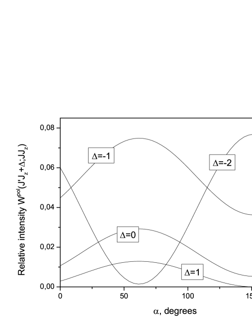
Figure 2: Relative intensities ${\mathcal{W}}^{\rm pol}(J^{\prime}J^{\prime}_{z};JJ_{z})$ of the Zeeman components $(JJ_{z})=(\frac{1}{2}\frac{1}{2})\rightarrow(J^{\prime}J^{\prime}_{z})=(\frac{3}{2}\frac{1}{2}+\Delta)$, $\Delta=-2,\ldots,1$ as function of $\alpha$ for randomly selected fixed values of the angles $\beta=72^{\circ},\theta=56^{\circ},\varphi=51^{\circ}$ (cf.  Eq. (32))

.

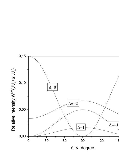
Figure 3: Relative intensities ${\mathcal{W}}^{\rm pol}(J^{\prime}J^{\prime}_{z};JJ_{z})$ of the Zeeman components $(JJ_{z})=(\frac{1}{2}\frac{1}{2})\rightarrow(J^{\prime}J^{\prime}_{z})=(\frac{3}{2}\frac{1}{2}+\Delta)$, $\Delta=-2,\ldots,1$, stimulated with linearly polarized laser light, as function of $\theta-\alpha$ for $\beta=45^{\circ}$ (cf. Eq. (33)).

			$A_{v^{\prime}L^{\prime}\rightarrow vL}$ (s-1)
$(vL)$	$(v^{\prime}L^{\prime})$	$\Delta E^{\rm NR}/hc\ (\mbox{cm}^{-1})$	$\bigl{|}\langle v^{\prime}L^{\prime}\|Q^{(2)}\|vL\rangle\bigr{|}/ea_{0}^{2}$	This work	Pilon Pilon2013
$(00)$	$(02)$	88.053	1.608226	0.30665[$-$12]	0.30665[$-$12]
$(00)$	$(12)$	1661.833	0.267274	0.20281[$-$07]	0.20281[$-$07]
$(00)$	$(22)$	3171.009	0.019403	0.27036[$-$08]	0.27036[$-$08]
$(00)$	$(32)$	4617.211	0.002497	0.29299[$-$09]	0.29298[$-$09]
$(00)$	$(42)$	6001.881	0.000451	0.35543[$-$10]
$(00)$	$(62)$	8591.673	0.000027	0.77727[$-$12]
$(01)$	$(11)$	1575.973	0.311496	0.35215[$-$07]	0.35215[$-$07]
$(01)$	$(21)$	3087.284	0.019765	0.40905[$-$08]	0.40905[$-$08]
$(01)$	$(31)$	4535.575	0.002284	0.37384[$-$09]	0.37382[$-$09]
$(01)$	$(41)$	5922.282	0.000367	0.36679[$-$10]
$(02)$	$(12)$	1573.782	0.340448	0.25064[$-$07]	0.25064[$-$07]
$(02)$	$(22)$	3082.958	0.021629	0.29183[$-$08]	0.29182[$-$08]
$(02)$	$(42)$	5913.830	0.000403	0.26277[$-$10]
$(03)$	$(11)$	1429.607	0.420823	0.39479[$-$07]	0.39479[$-$07]
$(04)$	$(12)$	1369.684	0.522608	0.29490[$-$07]
$(04)$	$(24)$	3067.885	0.027948	0.26415[$-$08]
$(04)$	$(32)$	4325.062	0.001717	0.99945[$-$10]	0.99939[$-$10]
$(06)$	$(56)$	7145.142	0.000129	0.26793[$-$11]
$(11)$	$(13)$	140.894	2.379256	0.50287[$-$11]	0.50287[$-$11]
$(11)$	$(33)$	3089.955	0.048979	0.10811[$-$07]	0.10811[$-$07]
$(20)$	$(42)$	2912.431	0.052069	0.12725[$-$07]
$(32)$	$(64)$	4135.286	0.024586	0.90959[$-$08]
$(52)$	$(54)$	167.679	4.033412	0.26834[$-$10]

Table 5: Nonrelativistic energies, $\Delta E^{\rm NR}=E^{{\rm(NR)}v^{\prime}L^{\prime}}\!-\!E^{{\rm(NR)}vL}$, reduced matrix elements, $|\langle v^{\prime}L^{\prime}||Q^{(2)}||vL\rangle\|$, of the electrical quadrupole moments, $Q^{(2)}$, Eq. (19), Einstein coefficients, $A_{v^{\prime}L^{\prime}\rightarrow vL}$ for selected $E2$ transitions between the ro-vibrational states $|vL\rangle$ and $|v^{\prime}L^{\prime}\rangle$ of ${\rm D_{2}^{+}}$, and, for comparison, the results of H.O. Pilon Pilon2013 when available.

Recent progress in the precision spectroscopy of the HD⁺ molecular ion Alighanbari-2020 has made it possible to resolve the Zeeman structure of laser induced $E1$ transition lines. This allowed to quantitatively study of the Zeeman and Stark shifts of the spectral lines, to reduce the related systematic uncertainties, and to determine the electron-to-proton mass ratio with improved accuracy. Anticipating the future precision spectroscopy of the D${}_{2}^{+}$ ion, we consider here some general characteristics of the Zeeman structure of laser-induces electric quadrupole transitions and reveal effects of the polarization of the stimulating laser light that appear only in higher multipolarity spectra. These effects are described by the factor ${\mathcal{W}}^{\rm pol}(J^{\prime}J^{\prime}_{z};JJ_{z})$ in Eq. (23) and impact the intensity and not the frequency of the $E2$ transition lines; the calculations of the Zeeman shift of the transition frequencies will be published elsewhere.

The cyclic components of the rank-2 irreducible tensor $\widehat{T}^{(2)}$ (20) are expressed in terms of the cartesian components as follows:

$$\begin{array}[]{@{}l}\displaystyle\widehat{T}^{(2)\pm 2}=\sqrt{\frac{1}{6}}\left(\hat{k}_{x}\hat{\epsilon}_{x}-\hat{k}_{y}\hat{\epsilon}_{y}\mp i\left(\hat{k}_{x}\hat{\epsilon}_{y}+\hat{k}_{y}\hat{\epsilon}_{x}\right)\right)\\[8.53581pt] \displaystyle\widehat{T}^{(2)\pm 1}=\sqrt{\frac{1}{6}}\left(\mp\left(\hat{k}_{x}\hat{\epsilon}_{z}+\hat{k}_{z}\hat{\epsilon}_{x}\right)+i\left(\hat{k}_{z}\hat{\epsilon}_{y}+\hat{k}_{y}\hat{\epsilon}_{z}\right)\right)\\[8.53581pt] \displaystyle\widehat{T}^{(2)0}=\frac{1}{3}\left(2\hat{k}_{z}\hat{\epsilon}_{z}-\hat{k}_{x}\hat{\epsilon}_{x}-\hat{k}_{y}\hat{\epsilon}_{y}\right)=\hat{k}_{z}\hat{\epsilon}_{z}.\end{array}$$ (31)

We have updated the normalization of these components as compared with Ref. Korobov2018 , but have kept unchanged the parametrization of the complex unit vector $\hat{\boldsymbol{\epsilon}}={\mathbf{E}}_{0}/|{\mathbf{E}}_{0}|$ pointing along the electric field amplitude ${\mathbf{E}}_{0}$. As in Korobov2018 , we denote by $K$ the lab reference frame with $z$-axis along the external magnetic field ${\mathbf{B}}$, by $K^{\prime}$ a reference frame with $z$-axis along $\hat{\bf k}$, and take the cartesian coordinates $(\epsilon^{\prime}_{x},\epsilon^{\prime}_{y},\epsilon^{\prime}_{z})$ of $\hat{\boldsymbol{\epsilon}}$ in $K^{\prime}$ to be $(\cos\theta,\sin\theta\,e^{i\varphi},0)$. Linear polarization of the incident light is described by $\varphi=0$; left/right circular polarization – by $\varphi=\pm\pi/2,\theta=\pi/4$; all other combinations correspond to general elliptic polarization. Let $(\alpha,\beta,\gamma)$ be the Euler angles of the rotation that transforms $K$ into $K^{\prime}$, and denote by $M(\alpha,\beta,\gamma)$ the matrix relating the cartesian coordinates $(a_{x},a_{y},a_{z})$ and $(a^{\prime}_{x},a^{\prime}_{y},a^{\prime}_{z})$ of an arbitrary vector ${\mathbf{a}}$ in $K$ and $K^{\prime}$, respectively: $a_{i}=\sum_{j}M_{ij}(\alpha,\beta,\gamma)\,a^{\prime}_{j}$. (To avoid mismatch of $M$ with $M^{-1}$, note that, e.g. $M_{xz}=-\sin\beta\,\cos\gamma$.) In this way, the absolute values of the components of $\widehat{T}$ in the lab frame $K$, appearing in Eq. (27) are parametrized with the four angles $\alpha,\beta,\theta$, and $\varphi$ (the dependence on $\gamma$ being cancelled):

$$\left|\widehat{T}^{(2)\pm 2}\right|^{2}= -\frac{1}{12}\sin^{4}\beta\,(1+\cos 2\alpha\,\cos 2\theta+\sin 2\alpha\,\sin 2\theta\,\cos\varphi)+$$ (32)

$$\frac{1}{6}\sin^{2}\beta(1\pm\cos\beta\,\sin 2\theta\,\sin\varphi)$$

$$\left|\widehat{T}^{(2)\pm 1}\right|^{2}= \frac{1}{12}+\frac{1}{24}\cos 2\beta\,(1-\cos 2\alpha\,\cos 2\theta)+\frac{1}{24}\cos 4\beta\,(1+\cos 2\alpha\,\cos 2\theta)-$$

$$\frac{1}{12}(1+2\cos 2\beta)\sin^{2}\beta\,\sin 2\alpha\,\sin 2\theta\,\cos\varphi\pm\frac{1}{6}\cos\beta\,\cos 2\beta\,\sin 2\theta\,\sin\varphi$$

$$\left|\widehat{T}^{(2)0}\right|^{2}= \frac{1}{8}\sin^{2}2\beta\,(1+\cos 2\alpha\,\cos 2\theta+\sin 2\alpha\,\sin 2\theta\,\cos\varphi)$$

This leads, for linear polarization ($\varphi=0$), to

$$\left|\widehat{T}^{(2)\pm 2}_{\rm lin}\right|^{2}= \frac{1}{6}\sin^{2}\beta\,(1-\sin^{2}\beta\,\cos^{2}(\theta-\alpha))$$ (33)

$$\left|\widehat{T}^{(2)\pm 1}_{\rm lin}\right|^{2}= \frac{1}{12}\,(1+\cos 4\beta\,\cos^{2}(\theta-\alpha)+\cos 2\beta\,\sin^{2}(\theta-\alpha))$$

$$\left|\widehat{T}^{(2)0}_{\rm lin}\right|^{2}= \frac{1}{4}\sin^{2}2\beta\,\cos^{2}(\theta-\alpha),$$

and for left circular polarization $(\theta=\pi/4,\varphi=\pi/2)$

$$\left|\widehat{T}^{(2)\pm 2}_{\rm left}\right|^{2}= \frac{1}{3}\sin^{2}\beta\,\left(\begin{matrix}\cos^{4}\frac{\beta}{2}\\ \sin^{4}\frac{\beta}{2}\end{matrix}\right)$$ (34)

$$\left|\widehat{T}^{(2)\pm 1}_{\rm left}\right|^{2}= \frac{1}{3}\,(1\mp 2\cos\beta)^{2}\left(\begin{matrix}\cos^{4}\frac{\beta}{2}\\ \sin^{4}\frac{\beta}{2}\end{matrix}\right)$$

$$\left|\widehat{T}^{(2)0}_{\rm left}\right|^{2}= \frac{1}{8}\sin^{2}2\beta.$$

For right circular polarization, described by $\theta=\pi/4$, $\varphi=-\pi/2$, the values of $|\widehat{T}^{(2)q}_{\rm right}|^{2}$ are obtained from the above expressions with the substitution $\left|\widehat{T}^{(2)q}_{\rm right}\right|^{2}=\left|\widehat{T}^{(2)-q}_{\rm left}\right|^{2}$.

Figure 4: Hyperfine structure of the $|01\rangle\rightarrow|11\rangle$ $E2$ vibrational transition line. The intensity of the hyperfine components ${\mathcal{W}}^{\rm hfs}$ is plotted against the laser frequency detuning $\Delta\omega/2\pi$ from the spin-averaged transition frequency. The spectrum is dominated by the “strong” (favored) components with $\Delta F=\Delta I=0$, while the intensity of transitions between hyperfine states with different $F$ or $I$ is suppressed by two orders of magnitude. The spectrum also includes a number of “weak” (unfavored) transitions with $\Delta F=+1$, not shown on the plot.

One might expect the intensity of the Zeeman components of the $E2$-transition spectrum to depend — as in $E1$ transitions — on three parameters only: one related to the laser polarization, and two more describing the mutual orientation of the external magnetic field ${\bf B}$ and the unit vectors $\hat{\mathbf{k}}$ and $\hat{\boldsymbol{\epsilon}}$. In fact, Eqs. (33) and (34) show that this is the case for circular and linear polarization only (when the difference $\theta-\alpha$ appears as a single parameter) while in the general case ${\mathcal{W}}^{\rm pol}(J^{\prime}J^{\prime}_{z};JJ_{z})$ depends substantially on both angles $\alpha$ and $\theta$. As an illustration, on Fig. 2 are plotted the relative intensities of the Zeeman components $|(vL)IFJ,J_{z}\rangle=|(00)0\frac{1}{2}\frac{1}{2},\frac{1}{2}\rangle\rightarrow|(12)0\frac{1}{2}\frac{3}{2},\frac{1}{2}+\Delta\rangle,\Delta=-2,-1,0,1$ as functions of $\alpha$ for the randomly selected values $\beta=72^{\circ},\theta=56^{\circ},\varphi=51^{\circ}$. The plot shows that the measurement of one or other individual Zeeman component of $E2$ transition lines may be substantially enhanced with appropriate optimization of the set-up geometry using Eqs. (32)-(34). The rather sharp dependence of the intensity of the individual Zeeman components on $\theta-\alpha$ for linear polarization and fixed value of the angle $\beta$ between ${\bf B}$ and the laser propagation direction (cf. Eq. (33)) is shown in Fig. 3.

III.3 Numerical results

$i$	$I$	$F$	$J$	$J^{\prime}$	$\Delta E^{\rm hfs}$ (MHz)	${\mathcal{W}}^{\rm hfs}$	$(d\Delta E^{\rm hfs}/dQ_{d})/h$ (kHz fm-2)
$(vL)=(00)\to(v^{\prime}L^{\prime})=(02)$
1	2	5/2	5/2	1/2	-40.018(11)	0.06648	-81.29
2	0	1/2	1/2	3/2	-32.093(2)0	0.40000	0.01
3	2	5/2	5/2	3/2	-25.426(11)	0.13244	-33.21
4	2	3/2	3/2	7/2	-12.456(16)	0.39882	-22.25
5	2	5/2	5/2	5/2	-6.961(11)	0.19868	26.03
6	2	3/2	3/2	5/2	-2.633(16)	0.29802	51.39
7	2	5/2	5/2	7/2	9.461(11)	0.26588	50.39
8	2	3/2	3/2	3/2	11.084(16)	0.19866	5.06
9	2	5/2	5/2	9/2	17.331(11)	0.33333	-28.14
10	0	1/2	1/2	5/2	21.395(1)0	0.60000	-0.02
11	2	3/2	3/2	1/2	22.814(16)	0.09973	-66.45
$(vL)=(00)\to(v^{\prime}L^{\prime})=(12)$
1	2	5/2	5/2	1/2	-40.975(11)	0.06649	-81.20
2	0	1/2	1/2	3/2	-30.692(2)0	0.40000	0.01
3	2	5/2	5/2	3/2	-27.064(11)	0.13249	-33.07
4	2	5/2	5/2	5/2	-9.415(11)	0.19875	26.07
5	2	3/2	3/2	7/2	-7.846(16)	0.39886	-22.19
6	2	3/2	3/2	5/2	1.587(16)	0.29812	51.32
7	2	5/2	5/2	7/2	6.318(11)	0.26591	50.33
8	2	5/2	5/2	9/2	13.883(11)	0.33333	-28.13
9	2	3/2	3/2	3/2	14.702(16)	0.19873	4.92
10	0	1/2	1/2	5/2	20.461(1)0	0.60000	-0.02
11	2	3/2	3/2	1/2	25.879(16)	0.09974	-66.51
$(vL)=(00)\to(v^{\prime}L^{\prime})=(22)$
1	2	5/2	5/2	1/2	-41.846(11)	0.06651	-80.80
2	0	1/2	1/2	3/2	-29.338(2)0	0.40000	0.01
3	2	5/2	5/2	3/2	-28.592(10)	0.13254	-32.80
4	2	5/2	5/2	5/2	-11.730(10)	0.19881	26.02
5	2	3/2	3/2	7/2	-3.474(16)	0.39892	-22.05
6	2	5/2	5/2	7/2	3.337(10)	0.26595	50.07
7	2	3/2	3/2	5/2	5.582(16)	0.29821	51.07
8	2	5/2	5/2	9/2	10.606(11)	0.33333	-28.02
9	2	3/2	3/2	3/2	18.115(16)	0.19881	4.76
10	0	1/2	1/2	5/2	19.559(1)0	0.60000	-0.02
11	2	3/2	3/2	1/2	28.759(16)	0.09976	-66.32
$(vL)=(01)\to(v^{\prime}L^{\prime})=(11)$
1	1	3/2	5/2	1/2	-33.061(5)0	0.29815	50.33
2	1	3/2	3/2	1/2	-22.787(5)0	0.04783	102.72
3	1	3/2	5/2	3/2	-11.612(5)0	0.41821	-52.31
4	1	1/2	1/2	3/2	-7.593(11)	0.98593	13.69
5	1	3/2	5/2	5/2	-1.754(5)0	0.28000	-0.00
6	1	3/2	3/2	3/2	-1.339(5)0	0.31375	0.08
7	1	1/2	3/2	3/2	2.913(11)	0.49218	-0.06
8	1	3/2	3/2	5/2	8.519(5)0	0.62718	52.39
9	1	1/2	3/2	1/2	12.973(10)	0.49305	-13.44
10	1	3/2	1/2	3/2	21.096(5)0	0.09564	-102.97
11	1	3/2	1/2	5/2	30.954(5)0	0.89412	-50.66

Table 6: The hyperfine shifts $\Delta E^{\rm hfs}/h=(\Delta E^{(v^{\prime}L^{\prime})IFJ^{\prime}}-\Delta E^{(vL)IFJ})/h$, in MHz, the relative intensities ${\mathcal{W}}^{\rm hfs}={\mathcal{W}}^{\rm hfs}((v^{\prime}L^{\prime})IFJ^{\prime};(vL)IFJ)$, and the derivative $(d\Delta E^{\rm hfs}/dQ_{d})/h$ for the ”strong” (favored) components in the hyperfine spectrum of two $E2$ transitions in D${}_{2}^{+}$. The transitions between stretched states are shown in boldface.

The rate ${\cal W}^{\rm NR}(v^{\prime}L^{\prime};vL)$ of laser stimulated $E2$ transitions between the ro-vibrational states $|vL\rangle$ and $|v^{\prime}L^{\prime}\rangle$ of the molecular ion D${}^{+}_{2}$ are expressed in Eq. (24) in terms of the reduced matrix elements $\langle v^{\prime}L^{\prime}\|Q^{(2)}\|vL\rangle$ of the electric quadrupole moment of D${}^{+}_{2}$ between these states. In the present work the reduced matrix elements were evaluated using the non-relativistic wave functions of D${}^{+}_{2}$ calculated in the variational approach of Ref. KorobovVarMethod . The numerical values needed for the evaluation of the rate of $E2$ transitions between a few selected ro-vibrational states are given in Table 5. For these transitions the table also lists the values of the Einstein’s coefficients $A_{v^{\prime}L^{\prime}\rightarrow vL}$, which are related to the reduced matrix elements by

$$A_{v^{\prime}L^{\prime}\rightarrow vL}/t_{0}^{-1}=\frac{\alpha^{5}}{15(2L+1)}((E^{{\rm NR}v^{\prime}L^{\prime}}-E^{{\rm NR}vL})/\mathcal{E}_{0})^{5}(\langle v^{\prime}L^{\prime}\|Q^{(2)}\|vL\rangle/ea_{0}^{2})^{2},$$ (35)

where $a_{0}$, $t_{0}=a_{0}/\alpha c$, and $\mathcal{E}_{0}=2{\rm Ry}$ are the atomic units of length, time, and energy. The comparison with the values calculated by H. O. Pilon Pilon2013 with different methods for a partly overlapping selection of transitions shows good agreement for the lower excited states, and indications of possible discrepancy of the order of $10^{-4}$ for the higher vibrational excitations. Juxtaposition with the analogous Table II of Ref. Korobov2018 shows that the rates of spontaneous transitions in D${}^{+}_{2}$ are suppressed in comparison with H${}_{2}^{+}$. This is mainly due to the smaller rotational and vibrational excitation energies, related to the larger nuclear mass. In addition to Table 5, the electronic supplement suppl gives the list of the reduced matrix elements for all $E2$ transitions between the ro-vibrational states with $v\leq 10$ and $L\leq 4$.

Further on, using the values of the amplitudes $\beta^{(vL)IFJ}_{I^{\prime}F^{\prime}}$, obtained by diagonalization of the effective spin Hamiltonian matrix (15), we calculated the coefficients ${\cal W}^{\rm hfs}((v^{\prime}L^{\prime})I^{\prime}F^{\prime}J^{\prime};(vL)IFJ)$, in the expression (23) for the rate of the individual hyperfine components. Fig. 4 illustrates the hyperfine structure of the $E2$ transition $|01\rangle\rightarrow|11\rangle$ and is representative also for other ro-vibrational transitions.

The spectrum consists of “strong” (favored) components between hyperfine states with the same values of the quantum numbers $F$ and $I$ spread over a range up to $\pm 50$ MHz around the center of gravity of the hyperfine manifold, and “weak” components between states with $\Delta F\neq 0$ or $\Delta I\neq 0$ at a distance of a few hundred MHz. The weak components are suppressed due to the relatively weak mixing of $F$ and $I$ in the eigenstates of the effective spin Hamiltonian matrix. Compared to H${}^{+}_{2}$, however, the suppression in D${}^{+}_{2}$ is less pronounced; the reason is that, because of the smaller nuclear magnetic moment of the deuteron, the contact spin-spin interactions dominate to a lesser extent thus leaving room for more $F$ and $I$ mixing.

Table 6 lists the details of the “strong” (favored) hyperfine components of four selected $E2$ transition lines: one rotational transition, two fundamental vibrational transitions, and one vibrational overtone transition. The electronic supplement suppl includes a table of the hyperfine structure of all $E2$ transition lines between the ro-vibrational states with $v\leq 10$ and $L\leq 4$.

III.4 Determining $Q_{d}$ by the composite frequency method

The currently available most accurate values of the deuteron electric quadrupole moment $Q_{d}$ have been obtained by combining the experimental results about the tensor interaction constant (traditionally denoted by $d$) in the $L=1$ state of the molecule D₂ from Ref. code with the high precision theoretical results about the electric field gradient at the nucleus of D₂, denoted by $q$ pavanello ; jozwiak ; komasa ; puchalski . The fractional uncertainty of the most recent of these results reported in Ref. puchalski – about $0.8\times 10^{-4}$ – comes from the fractional uncertainties of the experimental value of $d$ and theoretical value of $q$, $0.6\times 10^{-4}$ and $0.5\times 10^{-4}$, respectively. Hyperfine spectroscopy of the D${}_{2}^{+}$ ion offers the opportunity for an independent spectroscopic determination of $Q_{d}$. On the example of the purely rotational $E2$ transition $(vL)=(00)\to(v^{\prime}L^{\prime})=(02)$ we discuss the possibility to determine $Q_{d}$ using the composite frequency method PRL2014 ; traceless ; Alighanbari-2020 and the results of the present work as theoretical input, and estimate the accuracy of $Q_{d}$ that can be achieved this way.

We denote by “composite frequency” $\nu_{c}$ any linear combination of resonance frequencies $\nu_{i}$ of transitions between the ro-vibrational states $(vL)$ and $(v^{\prime}L^{\prime})$ of D${}_{2}^{+}$:

$$\nu_{c}=\sum\limits_{i=1}^{N}x_{i}\nu_{i},$$ (36)

where $x_{i}$ are numerical coefficients, normalized with $\sum\limits_{i=1}^{N}x_{i}^{2}=1$, whose values are to be determined by imposing appropriate additional conditions. The “experimental” value of the composite frequency is the linear combination of the experimental data: $\nu_{c}^{ex}=\sum\limits_{i=1}^{N}x_{i}\nu_{i}^{ex}$, while the “theoretical” value $\nu_{c}^{th}=\sum\limits_{i=1}^{N}x_{i}\nu_{i}^{th}$ is expressed in terms of the difference of the energy levels of the initial (lower) and final (upper) states of the transitions as defined in Eq. (6):

$$\nu_{i}^{th}=(E^{(v^{\prime}L^{\prime})I^{\prime}_{i}F^{\prime}_{i}J^{\prime}_{i}J^{\prime}_{zi}}-E^{(vL)I_{i}F_{i}J_{i}J_{zi}})/h=\nu^{th}_{\rm spin-avg}+\Delta E^{(v^{\prime}L^{\prime})I^{\prime}F^{\prime}J^{\prime}}-\Delta E^{(vL)IFJ},$$ (37)

$$\nu^{th}_{\rm spin-avg}=(E^{{\rm(diag)}v^{\prime}L^{\prime}}-E^{{\rm(diag)}vL})/h.$$

The quantity $\nu_{c}^{th}$ is a known function of the coefficients of the effective Hamiltonians for the initial and final states $E_{in},E^{\prime}_{in},n=1,...,6$, and indirectly – of the physical constants involved, including $Q_{d}$: $\nu_{c}^{th}=\nu_{c}^{th}(E_{in},E^{\prime}_{in},Q_{d})$. The value of $Q_{d}$ may be determined from the requirement that the theoretical value of the composite frequency be equal to the experimental one:

$$\nu_{c}^{th}(E_{in},E^{\prime}_{in},Q_{d})=\nu_{c}^{ex}$$ (38)

by resolving the latter with respect to $Q_{d}$: $Q_{d}=Q_{d}(E_{in},E^{\prime}_{in},\nu_{c}^{ex})$. We introduce the notations $\Gamma_{in}=E_{n}(\partial\nu_{i}^{th}/\partial E_{n})$, $(x\cdot\Gamma_{n})=\sum\limits_{i=1}^{N}x_{i}\Gamma_{in}$ (and similar for the “primed” symbols), where $\Gamma_{in}$ is the difference of the $\Gamma$’s defined in Eq. (17) for the final and initial state of the $i$-th transition: $\Gamma_{in}=\Gamma_{n}^{(v^{\prime}L^{\prime})I^{\prime}F^{\prime}J^{\prime}}-\Gamma_{n}^{(vL)IFJ}$. The absolute and fractional uncertainties $u(Q_{d}),u_{r}(Q_{d})$ of the quantity $Q_{d}$ arise from of the experimental uncertainty $u(\nu_{c}^{ex})$ of the experimental composite frequency $\nu_{c}^{ex}$ and from the theory uncertainties of the Hamiltonian coefficients $E_{n}$, $E^{\prime}_{n},n\leq 5$, $\bar{E}_{6}$, and $\bar{E}_{6}^{\prime}$. We denote their fractional uncertainties by $u_{n}$, $u^{\prime}_{n},n\leq 6$, respectively. Under the assumption that these uncertainties are uncorrelated, we obtain the following estimate of the fractional uncertainty $u_{r}(Q_{d})$ of $Q_{d}$:

$$u_{r}(Q_{d})=\frac{u(Q_{d})}{Q_{d}}=\sqrt{u_{r}^{th}(Q_{d})^{2}+u_{r}^{ex}(Q_{d})^{2}},$$

$$u_{r}^{th}(Q_{d})=\frac{\sqrt{\sum\limits_{n=1}^{6}\left((x\cdot\Gamma_{n})u_{n}\right)^{2}+\left((x\cdot\Gamma^{\prime}_{n})u^{\prime}_{n}\right)^{2}}}{\left|\left(x\cdot\Gamma_{6}\right)+\left(x\cdot\Gamma^{\prime}_{6}\right)\right|},\ u_{r}^{ex}(Q_{d})=\frac{u(\nu_{c}^{ex})}{\left|\left(x\cdot\Gamma_{6}\right)+\left(x\cdot\Gamma^{\prime}_{6}\right)\right|}$$ (39)

The coefficients $x_{i}$ are to be determined from the requirement that the fractional uncertainty $u_{r}(Q_{d})$ is minimal. Following the approach developed in Alighanbari-2020 we restrict the search for minima by imposing the constraint $\sum\limits_{i=1}^{N}x_{i}=0$ on the components of the vectors $x=\{x_{i}\}$. This suppresses the contribution from higher-order QED and relativistic spin-independent effects to the composite frequency.

As an illustration of the composite frequency approach, we estimate the accuracy with which the value of $Q_{d}$ could be retrieved from a measurement of the hyperfine structure of the $E2$ transition $(vL)=(00)\to(v^{\prime}L^{\prime})=(02)$. (The numerical estimates for the vibrational transitions $(00)\to(v^{\prime}2),v^{\prime}\geq 1$ are similar). The spectral line has 11 strong (favored) hyperfine components (see Table 6). For the initial state $(00)$ all coefficients $E_{n}$ but $E_{3}$ vanish (see Table 1). The numerical values of $\Gamma^{\prime}_{in},i=1,...,11,n=1,...,6$ and the non-vanishing $\Gamma_{i3}$ are given in Table 7.

Table 7: Numerical values of the nonvanishing derivatives $\Gamma_{i\alpha}\!=\!E_{\alpha}\left(\partial\nu_{i}/\partial E_{\alpha}\right)$ and $\Gamma^{\prime}_{i\alpha}\!=\!E^{\prime}_{\alpha}\left(\partial\nu_{i}/\partial E^{\prime}_{\alpha}\right)$ for the strong (favored) hyperfine components of the $(00)\to(02)$ transition line, in MHz. To ease comparison with Table 3, also given are the correspondent hyperfine shifts from the spin-averaged E2-transition frequency $\Delta E^{\rm hfs}/h$, in MHz. $a[b]$ stands for $a\times 10^{b}$.

$i$	$\Delta E^{\rm hfs}$	$\Gamma^{\prime}_{i1}$	$\Gamma^{\prime}_{i2}$	$\Gamma^{\prime}_{i3}$	$\Gamma^{\prime}_{i4}$	$\Gamma^{\prime}_{i5}$	$\Gamma^{\prime}_{i6}$	$\Gamma_{i3}$
1	-40.018	-0.28721[+2]	0.18094[$-$1]	0.14130[+3]	-0.10064[+2]	0.38755[$-$2]	-0.23231[$-$1]	-0.14253[+3]
2	-32.093	-0.32093[+2]	0.00000[+0]	-0.27500[$-$5]	0.50002[$-$7]	0.25000[$-$6]	0.29500[$-$5]	0.00000[+0]
3	-25.426	-0.20088[+2]	0.14551[$-$1]	0.13989[+3]	-0.27012[+1]	0.15840[$-$2]	-0.94920[$-$2]	0.14253[+3]
4	-12.456	-0.15585[+2]	-0.11915[$-$1]	-0.21236[+3]	0.17094[+1]	0.10605[$-$2]	-0.63596[$-$2]	0.21380[+3]
5	-6.961	-0.85783[+1]	0.82697[$-$2]	0.13993[+3]	0.42076[+1]	-0.12390[$-$2]	0.74380[$-$2]	-0.14253[+3]
6	-2.633	-0.21195[+1]	0.13370[$-$2]	-0.21107[+3]	-0.32599[+1]	-0.24500[$-$2]	0.14685[$-$1]	0.21380[+3]
7	9.461	0.48872[+1]	-0.89350[$-$3]	0.14122[+3]	0.58717[+1]	-0.24026[$-$2]	0.14401[$-$1]	-0.14253[+3]
8	11.084	0.93903[+1]	0.11065[$-$1]	-0.21103[+3]	-0.10894[+1]	-0.24250[$-$3]	0.14465[$-$2]	0.21380[+3]
9	17.331	0.21395[+2]	-0.12809[$-$1]	0.14228[+3]	-0.37906[+1]	0.13415[$-$2]	-0.80425[$-$2]	-0.14253[+3]
10	21.395	0.21395[+2]	0.00000[+0]	0.49999[$-$5]	0.10000[$-$6]	-0.60000[$-$6]	-0.68000[$-$5]	0.00000[+0]
11	22.814	0.18024[+2]	0.17128[$-$1]	-0.21244[+3]	0.34302[+1]	0.31675[$-$2]	-0.18990[$-$1]	0.21380[+3]

In absence of real spectroscopy data we assume in our considerations that the experimental uncertainty of the composite frequency $u(\nu_{c}^{ex})=\sqrt{\sum_{i=1}^{N}(x_{i}u(\nu_{i}^{ex}))^{2}}$ (where $u(\nu_{i}^{ex})$ are the uncertainties of the individual hyperfine lines) satisfies $1<u(\nu_{c}^{ex})<170$ Hz and focus our interest to this range; in agreement with Eq. (16) we take $u_{n}=u^{\prime}_{n}=\alpha^{2}\approx 5\times 10^{-5}$. In the range of interest, the uncertainty of $Q_{d}$ is determined – and limited – by the experimental uncertainty: the contribution of the term $u_{r}^{ex}(Q_{d})$ in Eq. (39) exceeds significantly $u_{r}^{th}(Q_{d})$ (see Table 9). The dependence of $u_{r}(Q_{d})$ on $u(\nu_{c}^{ex})$ is illustrated in Table 8. The uncertainty $u_{r}(Q_{d})$ decreases almost linearly with $u(\nu_{c}^{ex})$, and monotonously with the growth of the number $N$ of hyperfine lines included in the composite frequency $\nu_{c}$. However, beyond $N=6$ the advantage gained from adding more components $\nu_{i}$ is negligible (see Table 8). The optimal choice appears to be $N=6$; Table 9 lists the coefficients $x_{i},i=1,...,6$ in the optimal linear combination $\nu_{c}=\sum_{i}x_{i}\nu_{i},i\leq 6$ for a number of values of $u(\nu_{c}^{ex})$.

The above numerical estimates allow to outline the perspectives to determine $Q_{d}$ by means of spectroscopy of D${}_{2}^{+}$. For an experimental uncertainty $u(\nu_{c}^{ex})=42.4$ Hz as in the recently reported high precision pure rotational spectroscopy of HD⁺ Alighanbari-2020 , the resulting fractional uncertainty of $Q_{d}$, $u_{r}(Q_{d})\simeq 0.0015$, is nearly an order of magnitude smaller that what was obtained in HD⁺. To distinguish the values of $Q_{d}$ reported in Refs. komasa ; jozwiak , on the one hand, and in Refs. puchalski ; pavanello , on the other, the fractional uncertainty of $Q_{d}$ should be $u_{r}(Q_{d})\lesssim 10^{-3}$. Table 8 shows that this could be achieved using the theoretical results of the present work if $u(\nu_{c}^{ex})$ does not exceed 30 Hz – a level of experimental accuracy that has already been reached in HD⁺ spectroscopy, albeit so far only on a single transition Alighanbari-2020 . The accuracy of the extracted value of $Q_{d}$ would become competitive to the most precise available results if $u(\nu_{c}^{ex})$ could be reduced to $\sim 2$ Hz range. This is close to the experimental precision needed to extract $Q_{d}$ by direct comparison of the experimental and theoretical frequency of single hyperfine transitions (see Sec. II.3). However, only the composite frequency approach allows to reduce the theoretical error to a correspondingly low level.

It should be stressed that the efficiency of this approach depends on the type of transition: in transitions $(vL)\to(v^{\prime}L^{\prime})$ with $\Delta L=0$ the suppression of the theoretical uncertainty $u_{r}^{th}(Q_{d})$ is less pronounced. Also note that determining $Q_{d}$ from spectroscopy of HD⁺ with an uncertainty comparable to the values in Table 8 would only be possible with a significantly larger number $N$ of hyperfine components of the composite frequency compared to D${}_{2}^{+}$ spectroscopy.

Table 8: Achievable fractional uncertainty $u_{r}(Q_{d})$ of the electric quadrupole moment of the deuteron $Q_{d}$ if retrieved from a composite frequency for the $E2$ transition $(00)\to(02)$ versus the number $N$ of hyperfine components involved, for experimental uncertainties $u(\nu_{c}^{ex})$ between 170 and 1.3 Hz. $a[b]$ stands for $a\times 10^{b}$.

	Experimental uncertainty $u(\nu_{c}^{ex})$ (Hz)
$N$	169.6	84.8	42.4	21.2	10.6	5.3	2.6	1.3
4	0.57[-2]	0.34[-2]	0.23[-2]	0.19[-2]	0.10[-2]	0.60[-3]	0.44[-3]	0.39[-3]
5	0.53[-2]	0.28[-2]	0.15[-2]	0.85[-3]	0.48[-3]	0.29[-3]	0.16[-3]	0.10[-3]
6	0.52[-2]	0.27[-2]	0.15[-2]	0.80[-3]	0.42[-3]	0.22[-3]	0.12[-3]	0.76[-4]
7	0.51[-2]	0.27[-2]	0.15[-2]	0.79[-3]	0.41[-3]	0.21[-3]	0.12[-3]	0.75[-4]

Table 9: Theoretical, experimental, and overall fractional uncertainties $u_{r}^{th}(Q_{d})$, $u_{r}^{ex}(Q_{d})$, $u_{r}(Q_{d})$ of the deuteron quadrupole moment (see Eq. (39)), and coefficients $x_{i}$ of the optimal composite frequency $\nu_{c}$ of Eq. (36) for $N=6$, as function of the experimental uncertainty $u(\nu_{c}^{ex})$.

$u(\nu_{c}^{ex})$	$u_{r}(Q_{d})$	$u_{r}^{ex}(Q_{d})$	$u_{r}^{th}(Q_{d})$	Coefficients $x_{i}$ of the composite frequency $\nu_{c}$
(Hz)
169.6	0.52[-2]	0.51[-2]	0.11[-2]	$x_{1}\!=\!\phantom{-}0.32087$	$x_{4}\!=\!\phantom{-}0.14350$	$x_{5}\!=\!-0.10214$	$x_{6}\!=\!-0.70800$	$x_{7}\!=\!-0.21761$	$x_{11}\!=\!\phantom{-}0.56338$
84.8	0.27[-2]	0.26[-2]	0.91[-3]	$x_{1}\!=\!-0.31117$	$x_{4}\!=\!-0.18378$	$x_{5}\!=\!\phantom{-}0.15051$	$x_{6}\!=\!\phantom{-}0.72653$	$x_{7}\!=\!\phantom{-}0.15960$	$x_{11}\!=\!-0.54169$
42.4	0.15[-2]	0.14[-2]	0.56[-3]	$x_{1}\!=\!\phantom{-}0.28355$	$x_{2}\!=\!\phantom{-}0.11919$	$x_{4}\!=\!\phantom{-}0.12758$	$x_{5}\!=\!-0.35445$	$x_{6}\!=\!-0.69950$	$x_{11}\!=\!\phantom{-}0.52363$
21.2	0.80[-3]	0.77[-3]	0.22[-3]	$x_{1}\!=\!-0.33803$	$x_{2}\!=\!-0.25157$	$x_{3}\!=\!\phantom{-}0.21766$	$x_{5}\!=\!\phantom{-}0.27110$	$x_{6}\!=\!\phantom{-}0.64054$	$x_{11}\!=\!-0.53970$
10.6	0.42[-3]	0.41[-3]	0.99[-4]	$x_{1}\!=\!-0.38008$	$x_{2}\!=\!-0.24975$	$x_{3}\!=\!\phantom{-}0.32938$	$x_{5}\!=\!\phantom{-}0.20048$	$x_{6}\!=\!\phantom{-}0.61545$	$x_{11}\!=\!-0.51547$
5.3	0.22[-3]	0.21[-3]	0.61[-4]	$x_{1}\!=\!-0.39541$	$x_{2}\!=\!-0.24740$	$x_{3}\!=\!\phantom{-}0.37397$	$x_{5}\!=\!\phantom{-}0.16986$	$x_{6}\!=\!\phantom{-}0.60123$	$x_{11}\!=\!-0.50225$
2.7	0.12[-3]	0.11[-3]	0.54[-4]	$x_{1}\!=\!\phantom{-}0.11282$	$x_{2}\!=\!\phantom{-}0.40157$	$x_{5}\!=\!-0.47272$	$x_{6}\!=\!-0.61674$	$x_{9}\!=\!\phantom{-}0.11895$	$x_{11}\!=\!\phantom{-}0.45611$
1.3	0.76[-4]	0.53[-3]	0.54[-4]	$x_{1}\!=\!\phantom{-}0.11188$	$x_{2}\!=\!\phantom{-}0.40259$	$x_{5}\!=\!-0.47320$	$x_{6}\!=\!-0.61632$	$x_{9}\!=\!\phantom{-}0.11976$	$x_{11}\!=\!\phantom{-}0.45529$

III.5 Determining the spin-averaged frequency by the composite frequency method

Similar to the above, one may also seek a composite frequency that contains the spin-averaged frequency but minimizes the impact of the theory uncertainties of the HFS coefficients. This concept has been introduced in the experimental work of Ref. Alighanbari-2020 and in complementary form in Ref. traceless . For D${}_{2}^{+}$ this approach is particularly simple. As can be seen in Table 7, lines 2 and 10 are practically only sensitive to the coefficient $E^{\prime}_{1}$. Both the initial and final states for these transitions are nearly pure, with strongly suppressed admixture of other states, since the coupling through the terms with $E_{2}$, $E_{3}$, and $E_{4}$ of $H^{\rm eff}$ of Eq. (11) vanishes for $I=0$, and $|E_{5,6}|\ll|E_{1}|$. This yields the approximate expressions for the hyperfine shift of energy levels of these states: $\Delta E^{(vL)0FJ}\approx E_{1}(J(J+1)-F(F+1)-L(L+1))/2$, which are accurate to better than $10^{-5}$. Therefore, one can determine the spin-averaged frequency by

$$\nu_{\rm spin-avg}^{ex}=\frac{2}{5}\nu_{2}^{ex}+\frac{3}{5}\nu_{10}^{ex}.$$ (40)

The theoretical counterpart of this expression has 0.01 Hz uncertainty coming from the spin structure theory, negligible compared to the uncertainty coming from the QED theory. The same holds for the vibrational transitions $(0,0)\to(1,2)$ and $(0,0)\to(2,2)$. It is remarkable that only two spin transitions suffice to yield the spin-averaged frequency; this may be a significant advantage compared to HD⁺.

IV Conclusion

The present paper reports a series of new theoretical results about the spectroscopy of the molecular ion D${}_{2}^{+}$, including the most accurate to date calculations of the hyperfine structure of the lower excited ro-vibrational states with vibrational and rotational quantum numbers $v\leq 10$, $L\leq 4$. The correct theoretical treatment of the hyperfine structure is essential, considering that the experimental uncertainty of the measurement of the hyperfine structure has already reached the 20 Hz level in one of the molecular hydrogen ions Alighanbari-2020 . The paper also presents the first evaluation of the hyperfine structure of the $E2$ ro-vibrational transitions, and a thorough consideration of the laser polarization effects in the laser spectroscopy of the resolved Zeeman components of the hyperfine transition lines. The work closely followed, but also further developed the formalism of Ref. Korobov2018 for the study of the electric quadrupole transition spectrum of H${}^{+}_{2}$. The demonstrated efficiency of the composite frequency method underlines the perspectives for precision spectroscopy on D${}_{2}^{+}$ in the near future. Given the expected continued progress of experimental precision in trapped molecular ion spectroscopy, this work provides strong motivation for improving further the theoretical accuracy of the hyperfine coefficients and of the QED energies. Apart from the well-known goals of deuteron-to-electron mass ratio and electric quadrupole moment determination and test of QED, the spectroscopy of D${}_{2}^{+}$ specifically opens the possibility of searching for an anomalous force between deuterons salumbides2013 .

- (1) S. Schiller, D. Bakalov, and V.I. Korobov, Simplest Molecules as Candidates for Precise Optical Clocks, Phys. Rev. Lett. 113, 023004 (2014).
- (2) J.-Ph. Karr, H and HD+: candidates for a molecular clock, J. Mol. Spectrosc. 300, 37 (2014).
- (3) J.-Ph. Karr, L. Hilico, J. C. J. Koelemeij, and V. I. Korobov, Hydrogen molecular ions for improved determination of fundamental constants, Phys. Rev. A 94, 050501 (2016).
- (4) S. Alighanbari, M.G. Hansen, S. Schiller, and V.I. Korobov, Rotational spectroscopy of cold and trapped molecular ions in the Lamb-Dicke regime, Nature Physics 14, 555 (2018).
- (5) Sayan Patra, J.-Ph. Karr, L. Hilico, M. Germann, V.I. Korobov, and J.C.J. Koelemeij, Proton electron mass ratio from HD+ revisited, J. Phys. B: At. Mol. Opt. Phys. 51,2, 024003 (2018).
- (6) S. Alighanbari, G.S. Giri, F.L. Constantin, V.I. Korobov, and S. Schiller, Precise test of quantum electrodynamics and determination of fundamental constants with HD+ ions, Nature 580, 152 (2020), doi: https://doi.org/10.1038/s41586-020-2261-5.
- (7) Sayan Patra, M. Germann, J.-Ph. Karr, M. Haidar, L. Hilico, V.I. Korobov, F.M.J. Cozijn, K.S.E. Eikema, W. Ubachs, and J.C.J. Koelemeij, Proton-electron mass ratio from laser spectroscopy of HD+ at the part-per-trillion level, Science 369, 1238 (2020).
- (8) D.R. Bates and G. Poots, Properties of the Hydrogen Molecular Ion I: Quadrupole Transitions in the Ground Electronic State and Dipole Transitions of the Isotopic Ions, Proc. Phys. Soc. A 66, 784 (1953).
- (9) A. G. Posen, A. Dalgarno, and J. M. Peek, The quadrupole vibration-rotation transition probabilities of the molecular hydrogen ion, At. Data Nucl. Data Tables 28, 265 (1983).
- (10) H.O. Pilón and D. Baye, Quadrupole transitions in the bound rotational-vibrational spectrum of the hydrogen molecular ion, J. Phys. B: At. Mol. Opt. Phys. 45, 065101 (2012).
- (11) H.O. Pilón, Quadrupole transitions in the bound rotational-vibrational spectrum of the deuterium molecular ion, J. Phys. B: At. Mol. Opt. Phys. 46, 245101 (2013).
- (12) V.I. Korobov, P. Danev, D. Bakalov, and S. Schiller, Laser-stimulated electric quadrupole transitions in the molecular hydrogen ion H, Phys. Rev. A 97, 032505 (2018).
- (13) P. Zhang, Z. Zhong, and Z. Yan, Contribution of the deuteron quadrupole moment to the hyperfine structure of , Phys. Rev. A 88, 032519 (2013).
- (14) P. Zhang, Z. Zhong, Z. Yan, and T. Shi, Precision spectroscopy of the hydrogen molecular ion D, Phys. Rev. A 93, 032507 (2016).
- (15) J. F. Babb, The hyperfine structure of the hydrogen molecular ion, Talk at “PSAS-2008”, University of Windsor, Windsor, Ontario, Canada, July 21 - 26, 2008, http://web2.uwindsor.ca/psas/Full_Talks/Babb.pdf, unpublished.
- (16) H.A. Cruse,Ch. Jungen,and F. Merkt, Hyperfine structure of the ground state of para-D by high-resolution Rydberg-state spectroscopy and multichannel quantum defect theory, Phys. Rev. A 77, 042502 (2008).
- (17) A. Carrington, C.A. Leach, A.J. Marr, R.E. Moss, C.H. Pyne, and T.C. Steimle, Microwave spectra of the D and HD+ ions near their dissociation limits, J. Chem. Phys. 98, 5290 (1993).
- (18) J.F. Babb, The hyperfine structure of the hydrogen molecular ion, arXiv:physics/9701007 (1997).
- (19) J. F. Babb, Current Topics in Physics, eds.Y.M. Cho, J. B. Hong, and C. N. Yang (World Scientific, Singapore, 1998), p. 531.
- (20) M. Pavanello,W. C. Tung, and L. Adamowicz, Determination of deuteron quadrupole moment from calculations of the electric field gradient in D2 and HD, Phys. Rev. A 81, 042526 (2010).
- (21) H. Jozwiak, H. Cybulski, P. Wcislo, Hyperfine components of all rovibrational quadrupole transitions in the H2 and D2 molecules, arXiv:2006.05717 (2020).
- (22) J. Komasa, M. Puchalski, and K. Pachucki, Hyperfine structure in the HD molecule, arXiv:2005.02702 (2020).
- (23) S. Schiller and V.I. Korobov, Canceling spin-dependent contributions and systematic shifts in precision spectroscopy of molecular hydrogen ions, Phys. TRev. A 98, 022511 (2018).
- (24) M. Puchalski, J. Komasa, and K. Pachucki, Hyperfine structure of the first rotational level in H2, D2 and HD molecules and the deuteron quadrupole moment, arXiv:2010.06888 (2020).
- (25) D. Bakalov, S. Schiller, and V.I. Korobov, High-Precision Calculation of the Hyperfine Structure of the HD+ Ion, Phys. Rev. Lett. 97, 243001 (2006).
- (26) D. Bakalov, V.I. Korobov, and S. Schiller, Magnetic field effects in the transitions of the HD+ molecular ion and precision spectroscopy. J. Phys. B: At. Mol. Opt. Phys. 44, 025003 (2011).
- (27) V.I. Korobov, D. Bakalov, and H.J. Monkhorst, Variational expansion for antiprotonic helium atoms, Phys. Rev. A 59, R919(R) (1999).
- (28) https://physics.nist.gov/cuu/Constants/index.html.
- (29) See Supplemental Material at XXXXX for the numerical data related to the hyperfine structure of the rovibrational states of D with and and the spectrum of E2 transitions between them. .
- (30) R.F. Code and N.F. Ramsey, Molecular-beam magnetic resonance studies of HD and D2, Phys. Rev. A 4, 1945 (1971).
- (31) E.J. Salumbides, W. Ubachs, and V.I. Korobov, Bounds on fifth forces at the sub-Å length scale, J. Mol. Spectrosc. 300, 65 (2014).