The low-luminosity type II SN 2016aqf: A well-monitored spectral evolution of the Ni/Fe abundance ratio

Abstract

Low-luminosity type II supernovae (LL SNe II) make up the low explosion energy end of core-collapse SNe, but their study and physical understanding remain limited. We present SN 2016aqf, a LL SN II with extensive spectral and photometric coverage. We measure a $V$-band peak magnitude of $-14.58$ mag, a plateau duration of $\sim$100 days, and an inferred ⁵⁶Ni mass of $0.008\pm 0.002$ M_☉. The peak bolometric luminosity, L${}_{\rm bol}\approx 10^{41.4}$ erg s^-1, and its spectral evolution is typical of other SNe in the class. Using our late-time spectra, we measure the [O i] $\lambda\lambda 6300,6364$ lines, which we compare against SN II spectral synthesis models to constrain the progenitor zero-age main-sequence mass. We find this to be 12 $\pm$ 3 M_☉. Our extensive late-time spectral coverage of the [Fe ii] $\lambda 7155$ and [Ni ii] $\lambda 7378$ lines permits a measurement of the Ni/Fe abundance ratio, a parameter sensitive to the inner progenitor structure and explosion mechanism dynamics. We measure a constant abundance ratio evolution of $0.081^{+0.009}_{-0.010}$, and argue that the best epochs to measure the ratio are at $\sim$200 – 300 days after explosion. We place this measurement in the context of a large sample of SNe II and compare against various physical, light-curve and spectral parameters, in search of trends which might allow indirect ways of constraining this ratio. We do not find correlations predicted by theoretical models; however, this may be the result of the exact choice of parameters and explosion mechanism in the models, the simplicity of them and/or primordial contamination in the measured abundance ratio.

1 Introduction

Massive stars of $M\gtrsim 8$ M_☉ finish their lives with the collapse of their iron core, which releases great amounts of energy and produces explosions known as core collapse supernovae (CCSNe). These explosions can leave behind compact remnants in the form of neutron stars or black holes, although the exact details of the outcomes are not well understood. Within the different classes of CCSNe, type II SNe (SNe II), characterised by the presence of hydrogen in their spectra, are the most common (Li et al., 2011; Shivvers et al., 2017). SNe II are a heterogeneous class, with light curves showing different decline rates across a continuum (e.g., Anderson et al., 2014) from plateau (SNe IIP; with a pseudo-constant luminosity for $\sim$ 70 – 120 days) to linear decliners (SNe IIL, or fast-declining SNe). The light curves generally show two distinct phases: an optically-thick phase, driven by a combination of the expansion of the ejecta (which pushes the photosphere outwards) and the recombination of hydrogen (which pushes the photosphere inwards), and a later optically-thin phase, powered by the radioactive decay of ⁵⁶Co.

SNe II show a large diversity in luminosities, with peak $V$-band maximum absolute magnitudes ranging from $\sim-13.5$ to $\sim-19$ mag, and an average of about $-16.7$ mag ($\sigma$ = 1.01 mag; Anderson et al., 2014). Several low-luminosity SNe II (LL SNe II), generally events with $V\gtrsim-16$ mag (e.g., Kulkarni & Kasliwal, 2009; Smartt et al., 2015, see also Gal-Yam 2017; however, note that Pastorello 2012 proposes an alternative definition), have been found in the past decades (e.g., Turatto et al., 1998; Pastorello, 2012; Spiro et al., 2014; Lisakov et al., 2018).

The prototype of this faint sub-class is SN 1997D (de Mello et al., 1997; Turatto et al., 1998). SN 1997D displayed a low luminosity and low expansion velocity. However, it was discovered several weeks after peak, with no well-constrained explosion epoch. The first statistical study of this sub-class was that of Pastorello et al. (2004), who found the class to be characterised by narrow spectral lines (P-Cygni profiles) and low expansion velocities (a few $1000$ km s^-1 during the late photospheric phase), suggesting low explosion energies ($E_{\rm exp}\lesssim$ few times $10^{50}$ erg). Their bolometric luminosity during the recombination ranges between $\sim 10^{41}$ erg s^-1 and $\sim$ $10^{42}$ erg s^-1, with SN 1999br (Pastorello et al., 2004) and SN 2010id (Gal-Yam et al., 2011) being the faintest SNe II discovered. They also show lower exponential decay luminosity than the bulk of SNe II, which reflects their low ⁵⁶Ni masses (M_Ni $\lesssim 10^{-2}$ M_☉), in agreement with the low explosion energies as expected from the M_Ni-$E_{\rm exp}$ relation found in different studies (e.g., Pejcha & Prieto, 2015; Kushnir, 2015; Müller et al., 2017). Spiro et al. (2014) have since expanded the statistical study of LL SNe II, adding several objects and finding similar characteristics to those found by Pastorello et al. (2004). While the current sample of nebular spectra of LL SNe II is growing, the study of additional events with better cadence and higher signal-to-noise data is essential for understanding their observed diversity.

The progenitors of LL SNe II have been shown to be red supergiants (RSGs) with relatively small Zero Age Main Sequence (ZAMS) masses ($M\lesssim 15$ M_☉) using archival pre-SN imaging (e.g. Smartt et al., 2009; Smartt, 2015) and hydrodynamical models (e.g. Dessart et al., 2013b; Martinez & Bersten, 2019). However, other studies have suggested the possibility that their progenitors are more massive RSGs with large amounts of fallback material (e.g. Zampieri et al., 2003). Theoretical studies have shown that the nebular [O i] $\lambda\lambda 6300,6364$ doublet is a good tracer of the progenitor core mass, and, therefore, of the progenitor ZAMS mass (e.g., Jerkstrand et al., 2012, 2014, 2018, hereafter J12, J14 and J18; and some other studies as well, e.g., Lisakov et al. 2017, 2018), making the late-time spectral evolution extremely important for the study of SN progenitors. Furthermore, nebular nucleosynthesis diagnosis is so far consistent with the lack of massive progenitors above $\sim$20 M_☉ (e.g. J14, Jerkstrand et al. 2015a; Valenti et al. 2016).

In addition to the study of the nebular [O i] $\lambda\lambda 6300,6364$ doublet as progenitor mass estimator, the Ni/Fe abundance ratio, measured from the [Fe ii] $\lambda 7155$ and [Ni ii] $\lambda 7378$ lines, have been shown to be important for the understanding of the inner structure of the progenitor and the explosion mechanism dynamics, as the observed iron-group yields are linked to the temperature, density and neutron excess of the layers that become fuel for the rapid burning process of the explosion (Jerkstrand et al., 2015a, b, hereafter J15a, J15b). However, there are few studies of this ratio, mainly due to the lack of late-time spectra and the absence of these features in the available data in the literature.

In this paper, we study SN 2016aqf: a well-observed (i.e., excellent spectral and photometric coverage) LL SN II, discovered soon after explosion, with $M_{V}^{\mathrm{max}}=-14.58$ mag, a plateau duration of $\sim$ 100 days and a measured M_Ni $=0.0010$ M_☉ (see Sec. 3.2 and 4.1). The nebular spectra show the [O i] $\lambda\lambda 6300,6364$ doublet. The He i $\lambda 7065$ emission line is also seen in the spectra of SN 2016aqf, a line associated to SNe with a low progenitor mass, but not present in every LL SN II and not well understood. In addition, SN 2016aqf is one of the few cases where the [Fe ii] $\lambda 7155$ and [Ni ii] $\lambda 7393$ lines (produced by ⁵⁶Ni and ⁵⁸Ni, respectively) can be seen in the nebular spectra ($\sim$ 150 – 330 days after the explosion) over $\sim$ 170 days. This extended coverage of the Ni/Fe abundance ratio presents a unique opportunity to study its evolution, and serves as a test for current late-time spectral modelling as well as providing a rich legacy dataset.

This paper is structured as follows: in Sec. 2.1 we describe the observations, data reduction and host galaxy of SN 2016aqf. In Sec. 3 we show the light curve, colour and spectral evolution of SN 2016aqf and compare it with other LL SNe II. In Sec. 4 we estimate the physical parameters of SN 2016aqf, while in Sec. 5 we discuss our findings. Finally, our conclusions are in Sec. 6. Throughout this paper we assume a flat $\Lambda$CDM cosmology with $H_{0}=70$ km s^-1 Mpc^-1, $\Omega_{\mathrm{M}}=0.3$ and $\Omega_{\Lambda}=0.7$, as these values are widely used in the literature (e.g., Gutiérrez et al., 2018) and the $H_{0}$ value lies between the value measured from the CMB (Planck Collaboration et al., 2016) and local measurements (e.g., Riess et al., 2018).

2 Observations, reductions and host galaxy

2.1 SN Photometry and Spectroscopy

SN 2016aqf (ASASSN-16cc) was discovered on 2016 February 26 at 04:33:36 UTC (57444.19 MJD) by the All-Sky Automated Survey for Supernovae (ASAS-SN; Shappee et al., 2014) at RA = 05h46m23$\aas@@fstack{s}$91 and Dec. = $-$52°05′18$\aas@@fstack{\prime\prime}$9, in NGC 2101 (Brown et al., 2016) at $z=0.004016$ (Lauberts & Valentijn, 1989). On 2016 February 27, SN 2016aqf was classified as a SN II (Hosseinzadeh et al., 2016; Jha & Miszalski, 2016). Based on the low luminosity of the host ($M_{B}=-17.66$ mag as in Gutiérrez et al. 2018, although see Sec. 2.2), we commenced a follow-up campaign with the extended Public ESO Spectroscopic Survey of Transient Objects (ePESSTO) as part of the programme ‘SNe II in Low-luminosity host galaxies’.

The final pre-explosion non-detection in the $V$-band, reported three days before the date of classification by ASAS-SN (57442 MJD), has a limiting magnitude $\sim 16.7$ mag, which does not give a stringent constraint on the explosion epoch. Previous non-detections have similar limiting magnitudes. Hence, we decided to estimate the explosion epoch using the spectral matching technique (e.g., Anderson et al., 2014; Gutiérrez et al., 2017). We used gelato (Harutyunyan et al., 2008) to find good spectral matches to the highest resolution spectrum of SN 2016aqf, as it is also one of the first spectra taken (57446 MJD, see below). From the best matching templates, we calculated a mean epoch of the spectrum of $\sim$6 days after explosion and a mean error added with the standard deviation of the explosion epochs in quadrature of $\sim$ 4 days. This gives an explosion epoch of MJD $57440.19\pm 4$ (slightly different to the estimated epoch in Gutiérrez et al. 2018 as they used the non-detection)

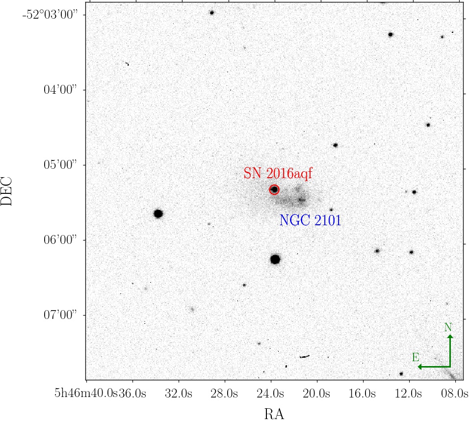
Figure 1: $r$-band image of NGC 2101 with SN 2016aqf marked. Data from the 1.0-m Las Cumbres Observatory telescopes (MJD = 57514, 74 days after explosion).

Optical $BVgri$ imaging of SN 2016aqf was obtained with the 1.0-m telescope network of the Las Cumbres Observatory (LCO; Brown et al., 2013) as part of both ePESSTO and the ‘Las Cumbres Observatory SN Key Project’, with data taken from 8 to 311 d after explosion. All photometric data were reduced following the prescriptions described by Firth et al. (2015). This pipeline subtracts a deep reference image constructed using data obtained in the $BVgri$ bands three years after the first detection of SN 2016aqf to remove the host-galaxy light using a point-spread-function (PSF) matching routine. SN photometry is then measured from the difference images using a PSF-fitting technique. Fig. 1 shows the SN position within the host galaxy. The photometry of SN 2016aqf is presented in Table 1.

Table 1: SN 2016aqf $BVgri$-band photometry between +5 and +311 days. $BV$ bands are in Vega magnitude system, while $gri$ bands are in AB magnitude system.

MJD	Phase	$B$	$\sigma_{B}$	$V$	$\sigma_{V}$	$g$	$\sigma_{g}$	$r$	$\sigma_{r}$	$i$	$\sigma_{i}$
57448	8	15.851	0.006	15.851	0.006	15.851	0.006	15.851	0.006	15.851	0.006
57452	12	15.985	0.005	15.985	0.005	15.985	0.005	15.985	0.005	15.985	0.005
57455	15	16.057	0.010	16.057	0.010	16.057	0.010	16.057	0.010	16.057	0.010
57456	16	16.045	0.034	16.045	0.034	16.045	0.034	16.045	0.034	16.045	0.034
57457	17	16.033	0.103	16.033	0.103	-	-	-	-	-	-
57458	18	16.095	0.039	16.095	0.039	16.095	0.039	16.095	0.039	-	-
57459	19	16.131	0.008	16.131	0.008	16.131	0.008	16.131	0.008	16.131	0.008
57460	20	16.190	0.005	16.190	0.005	16.190	0.005	16.190	0.005	16.190	0.005
57462	22	16.268	0.031	16.268	0.031	16.268	0.031	16.268	0.031	16.268	0.031
57468	28	16.459	0.009	16.459	0.009	16.459	0.009	16.459	0.009	16.459	0.009
57474	34	16.534	0.010	16.534	0.010	16.534	0.010	16.534	0.010	16.534	0.010
57480	40	16.576	0.008	16.576	0.008	16.576	0.008	16.576	0.008	16.576	0.008
57487	47	16.650	0.009	16.650	0.009	16.650	0.009	16.650	0.009	16.650	0.009
57493	53	16.754	0.015	16.754	0.015	16.754	0.015	16.754	0.015	16.754	0.015
57499	59	16.812	0.014	16.812	0.014	16.812	0.014	16.812	0.014	16.812	0.014
57505	65	16.824	0.015	16.824	0.015	16.824	0.015	16.824	0.015	16.824	0.015
57512	72	16.890	0.017	16.890	0.017	-	-	16.890	0.017	16.890	0.017
57514	74	16.912	0.012	16.912	0.012	16.912	0.012	16.912	0.012	16.912	0.012
57523	83	-	-	-	-	16.258	0.007	16.258	0.007	-	-
57524	84	-	-	-	-	16.289	0.008	16.289	0.008	-	-
57526	86	17.182	0.030	17.182	0.030	17.182	0.030	17.182	0.030	17.182	0.030
57598	158	19.108	0.034	19.108	0.034	19.108	0.034	19.108	0.034	19.108	0.034
57617	177	19.216	0.095	19.216	0.095	19.216	0.095	19.216	0.095	19.216	0.095
57684	244	20.311	0.041	20.311	0.041	20.311	0.041	20.311	0.041	20.311	0.041
57704	264	20.430	0.074	20.430	0.074	20.430	0.074	20.430	0.074	20.430	0.074
57726	286	-	-	19.546	0.077	19.546	0.077	-	-	-	-
57727	287	-	-	-	-	19.795	0.049	19.795	0.049	19.795	0.049
57728	288	20.709	0.063	20.709	0.063	20.709	0.063	20.709	0.063	20.709	0.063
57749	309	20.925	0.120	20.925	0.120	20.925	0.120	20.925	0.120	20.925	0.120
57750	310	20.717	0.073	20.717	0.073	20.717	0.073	20.717	0.073	20.717	0.073
57751	311	20.932	0.076	20.932	0.076	20.932	0.076	20.932	0.076	20.932	0.076

Spectroscopic observations were obtained with the ESO Faint Object Spectrograph and Camera version 2 (EFOSC2; Buzzoni et al., 1984) at the 3.58-m ESO New Technology Telescope (NTT), the FLOYDS spectrograph (Brown et al., 2013) on the Faulkes Telescope South (FTS), and the Robert Stobie Spectrograph (RSS; Burgh et al. 2003; Kobulnicky et al. 2003) at the Southern African Large Telescope (SALT). FLOYDS spectra were taken as part of the ‘Las Cumbres Observatory SN Key Project’. The observations include phases from 2 to 348 d after explosion. EFOSC2 spectra, obtained with grism #13, cover 3500–9300 Å at a 21.2 Å resolution, the FLOYDS spectra have wavelength coverage of $\sim$ 3200 – 10000 Å with a resolution of $\sim 18$ Å, and the RSS spectrum (Jha & Miszalski, 2016) covers 3600–9200 Å at $\sim 7$ Å resolution. The data reduction of the EFOSC2 spectra was performed using the PESSTO pipeline (Smartt et al., 2015), while the FLOYDS data were reduced using the pyraf-based floydsspec pipeline (Valenti et al., 2014). All spectra are available via the WISeREP repository (Yaron & Gal-Yam, 2012). Spectral information is summarised in Table 2.

Table 2: The UTC dates mark the beginning of the exposures. Phase with respect to the explosion epoch (MJD 57440.19).

UTC Date	MJD	Phase	Range [Å]	Resolution [Å]	Telescope/Instrument
2016-02-27T09:54:44.475	57445.4	5	3250 - 9300	18.0	FTS/FLOYDS-S
2016-02-27T21:00:25.837	57445.9	6	3600 - 9200	7.0	SALT/RSS
2016-03-01T11:24:32.205	57448.5	8	3250 - 10000	18.0	FTS/FLOYDS-S
2016-03-06T10:09:18.022	57453.4	13	3300 - 10001	18.0	FTS/FLOYDS-S
2016-03-09T04:39:49.731	57456.2	16	3640 - 9235	21.2	NTT/EFOSC2
2016-03-10T12:46:20.372	57457.5	17	3299 - 10000	18.0	FTS/FLOYDS-S
2016-03-15T10:13:25.851	57462.4	22	3250 - 10000	18.0	FTS/FLOYDS-S
2016-03-22T11:10:18.554	57469.5	29	3900 - 9999	18.0	FTS/FLOYDS-S
2016-03-30T09:29:37.393	57477.4	37	3401 - 10000	18.0	FTS/FLOYDS-S
2016-04-06T08:58:10.460	57484.4	44	3299 - 9999	18.0	FTS/FLOYDS-S
2016-04-13T10:06:55.453	57491.4	51	3599 - 10000	18.0	FTS/FLOYDS-S
2016-04-15T08:39:52.609	57493.4	53	3600 - 10000	18.0	FTS/FLOYDS-S
2016-04-16T00:26:16.687	57494.1	54	3645 - 9239	21.2	NTT/EFOSC2
2016-04-22T08:55:30.146	57500.4	60	3950 - 10000	18.0	FTS/FLOYDS-S
2016-05-04T09:27:45.944	57512.4	72	3650 - 10000	18.0	FTS/FLOYDS-S
2016-07-26T09:49:26.448	57595.4	155	3645 - 9239	21.2	NTT/EFOSC2
2016-08-08T09:39:55.699	57608.4	168	3639 - 9233	21.2	NTT/EFOSC2
2016-09-11T08:20:03.866	57642.3	202	3640 - 9233	21.2	NTT/EFOSC2
2016-09-29T07:23:09.743	57660.3	220	3636 - 9232	21.2	NTT/EFOSC2
2016-11-07T07:57:09.799	57699.3	259	3639 - 9232	21.2	NTT/EFOSC2
2016-11-19T04:31:19.658	57711.2	271	3636 - 9231	21.2	NTT/EFOSC2
2016-12-03T06:56:26.427	57725.3	285	3639 - 9232	21.2	NTT/EFOSC2
2016-12-21T05:55:04.628	57743.2	303	3640 - 9233	21.2	NTT/EFOSC2
2017-01-17T02:55:39.708	57770.1	330	3639 - 9233	21.2	NTT/EFOSC2
2017-02-07T02:46:40.051	57791.1	351	3640 - 9233	21.2	NTT/EFOSC2

2.2 Host Galaxy

Photometry of NGC2101 was obtained with the LCO 1.0-m telescope network, and spectroscopy with VLT/FORS2, around three years after the SN explosion (2019 February 6 at 04:38:48 UTC). We estimated a galaxy distance of $\mu=30.16\pm 0.27$ mag (see Sec. 3.2), consistent with the Tully-Fisher value of $\mu=30.61\pm 0.80$ mag, as reported in the NASA/IPAC Extragalactic Database (NED). Adopting the distance estimated in this work, the galaxy has $M_{B}$ = $-17.22\pm 0.34$ mag, which is consistent with the value reported in Gutiérrez et al. (2018, $-17.66$ mag) given the large uncertainties from the reported distance. We use the total apparent corrected $B$-magnitude, with the total B-magnitude error as reported in HyperLEDA, using error propagation. The radial velocity corrected for Local Group infall onto Virgo is $883\pm 3$ km s^-1 (Theureau et al., 1998; Terry et al., 2002), as reported in HyperLEDA, a value which we use to estimate the corrected redshift of SN 2016aqf.

From the spectrum of the H ii region at the position of the SN, we measure the emission line fluxes of H $\alpha$, H $\beta$, [N ii] and [O iii]. We estimate the star-formation rate (SFR) from the H$\alpha$ line as SFR = $2.3\pm 0.6\times 10^{-1}$ M_☉ yr^-1 using the calibration from Kennicutt & Evans (2012), where the uncertainty is driven by the uncertainty in the distance. Using the calibration of Marino et al. (2013), we then estimate a gas-phase metallicity of (12 + log(O/H))${}_{\rm O3N2}=8.144\pm 0.025$ dex and (12 + log(O/H))${}_{\rm N2}=8.134\pm 0.042$ dex, i.e., below the solar value of 8.69 dex (Asplund et al., 2009). This is low compared to many other SN II host galaxies, but not uncommon (e.g., Anderson et al., 2016). However, the metallicity does not follow the relation found with the Fe ii $\lambda 5018$ pEW (e.g., Dessart et al., 2014; Anderson et al., 2016; Gutiérrez et al., 2018). This may be caused by the lower temperatures in LL SNe II which causes the earlier appearance of the Fe ii lines in these objects (Gutiérrez et al., 2017).

3 Results and analysis

3.1 Extinction corrections

We adopt a Milky Way extinction value of $E(B-V)_{\mathrm{MW}}=0.047$ mag, and correct our photometry using the prescription of Schlafly & Finkbeiner (2011) and the Cardelli et al. (1989) reddening law with $R_{V}=3.1$. To estimate the host galaxy extinction, we investigated the equivalent-width (EW) of the Na i D ($\lambda\lambda 5889,5895$) absorption, a well-known tracer of gas, metals and dust (e.g., Richmond et al., 1994; Munari & Zwitter, 1997; Turatto et al., 2003; Poznanski et al., 2012). We note that these relations tend to have large uncertainties.

The spectrum at +6 d is the only one that seems to shows Na i D absorption lines from the MW and the host galaxy. We used the relations for one line (D₁) and two lines (D₁+D₂) from Poznanski et al. (2012), obtaining upper limits of $E(B-V)\lesssim 0.028\pm 0.011$ mag and $E(B-V)\lesssim 0.032\pm 0.006$ mag, respectively. This gives a weighted average value of $E(B-V)\lesssim 0.031$ mag. Given this very small level of extinction (and its uncertainty), we choose not to make an extinction correction to the SN data. We do not use other methods to estimate this value as they rely on the SN colour; de Jaeger et al. (2018) showed that the majority of colour dispersion of SNe II is intrinsic to the SN.

3.2 Light curve and distance

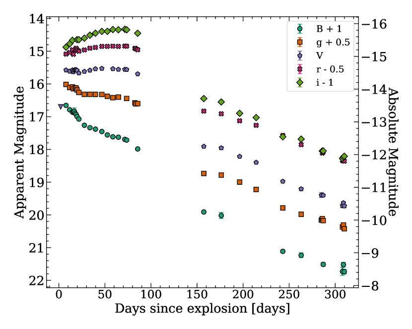
Figure 2: SN 2016aqf $BVgri$-band photometry from +8 to + 311 d. $BV$ bands are in Vega magnitude system, while $gri$ bands are in AB magnitude system. The last non-detection in $V$ band is also shown (inverted triangle). The SN was not visible around the transition from the optically-thick to the optically-thin phase. Offsets have been applied to the photometry for visualisation purposes. As in all figures in this paper, the photometry is corrected for MW extinction but not host extinction, and the data are in the rest-frame.

The $BVgri$-band light curves of SN 2016aqf (Fig. 2) cover 8 to 311 d after explosion (all phases in this paper are relative to the estimated explosion epoch). As the host galaxy is not in the Hubble flow, we estimated the distance to SN 2016aqf using the Standardized Candle Method (Hamuy & Pinto, 2002), which relates the velocity of the ejecta of a SN II to its luminosity during the plateau, and the relation of Kasen & Woosley (2009, equation 17) for a redshift-independent distance estimate. We calculate the distance modulus $\mu=30.16\pm 0.27$ mag ($10.8\pm 1.4$ Mpc), which gives $M_{V}^{\mathrm{max}}=-14.58$ mag and a mid-plateau $V$-band luminosity of $-14.63$ mag (note the plateau luminosity is slightly brighter; $M_{V}^{\rm max}$ represents the maximum luminosity from the peak closest to the bolometric peak). We estimated $M_{V}^{\rm max}$ from the first epoch of photometry given that the last non-detection helps to obtain a good constrain.

During the recombination phase, the SN shows an increase in the $Vri$-bands luminosity, probably due to its low temperature which shifts the peak luminosity from the ultraviolet (UV) to redder bands more rapidly compared to normal SNe II. The gap in observations between 80 and 150 days was caused by the SN going behind the sun, and coincides with the SN transitioning from the optically-thick to the optically-thin phase. The $V$-band decreases by $\sim 2$ mag across the gap in the light curve, and is an estimate of the decrease caused by the transition from plateau to nebular phase, smaller than other LL SNe II ($\sim 3$–$5$ mag; e.g., Spiro et al., 2014). We measured the decline rate in the $V$-band at early epochs ($t\lesssim 20$ days; $s_{1}$), in the plateau ($s_{2}$), and in the exponential decay tail ($s_{3}$) as defined in Anderson et al. (2014, see section 4.2 for the $t_{\rm pt}$ used), obtaining $s1=0.65_{-0.12}^{+0.13}$ mag 100 d^-1, $s2=-0.08_{-0.01}^{+0.01}$ mag 100 d^-1 and $s3=1.22_{-0.02}^{+0.02}$ mag 100 d^-1. $M_{\rm tail}$ was not measured as the early decline of the exponential decay tail was not observed.

3.3 Colour Evolution

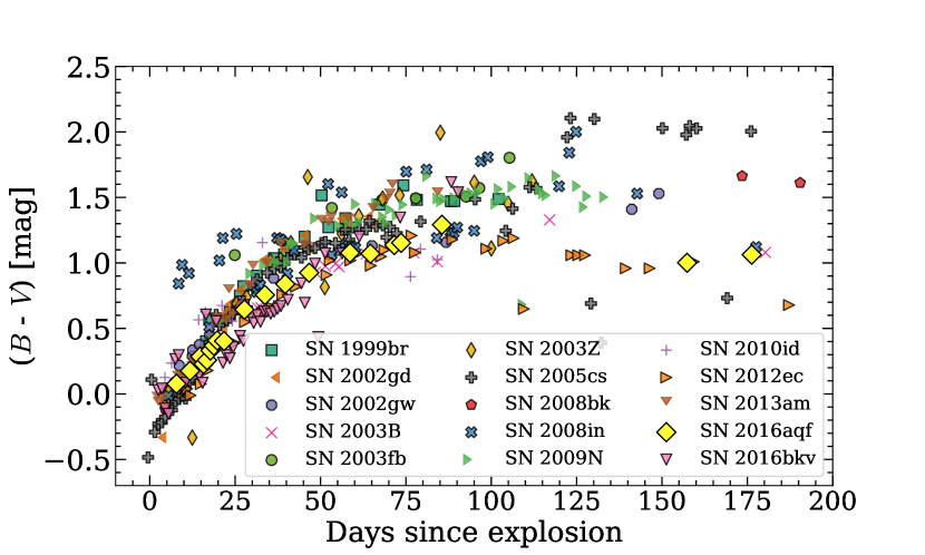
Figure 3: ($B$-$V$) colour evolution of SN 2016aqf compared to our sample of LL SNe II. All data is corrected for MW and host galaxy extinction (except for those SNe with host extinction values reported as upper limits in Table 3.) Notice that the dispersion generally increases with time. Uncertainties are not shown as they are relatively small in general.

In Fig. 3 we show the ($B-V$) colour curve (corrected for MW extinction) of SN 2016aqf during the first 200 days. At the beginning of the observations ($8$ d) it has a colour close to $0$ mag, which slowly increases to around $1.0$ mag at $\sim+50$ d and $\sim 1.3$ mag before the gap in coverage.

For comparison, we form a sample of other LL SNe II from the literature with good data coverage and similar properties to our object: SN 1999br (Hamuy, 2003; Pastorello et al., 2004; Gutiérrez et al., 2017), SN 2002gd, SN 2002gw , SN 2003B, SN 2003fb, SN 2003Z, SN 2004fx, SN 2005cs, SN 2008bk, SN 2008in, SN 2009N, SN 2010id, SN 2013am and SN 2016bkv. These SNe and their references are in Table 3. In addition we include SN 2012ec (Maund et al., 2013), a non-LL SN II, as a reference as it has a well-measured Ni/Fe abundance ratio, used in our later analysis. For this comparison sample, we use photometry and spectra obtained from the ‘Open Supernova Catalog’ (Guillochon et al., 2017) and WISeREP (Yaron & Gal-Yam, 2012). Note that we only used epochs with both $B$ and $V$ photometry to calculate colour, without applying interpolations. The photometry of this sample is corrected for MW extinction (see Sec. 3.1), and host galaxy extinction, using the values from the references in Table 3. However, we do not correct for host galaxy extinction when the reported value is an upper limit (this does not represent a problem given the relatively small extinction values, A_V < 0.1 mag).

Table 3: SN II sample used throughout this work. The data for this sample were taken from the references cited in column References.

SN	z	MNi	$\sigma_{\rm Ni}^{-}$	$\sigma_{\rm Ni}^{+}$	$\mu$	$\sigma_{\mu}$	$A_{V}$(MW)	$A_{V}$(Host)	Host	References
		[M⊙]	[M⊙]	[M⊙]	[mag]	[mag]	[mag]	[mag]
SN1997D	0.004059	0.005	0.004	0.004	30.74	0.92	0.057	$\lesssim$0.060	NGC 1536	Turatto et al. (1998), Zampieri et al. (2003)
										Spiro et al. (2014)
SN1999br	0.00323	0.002	0.001	0.001	30.97	0.83	0.063	0.000	NGC 4900	Hamuy (2003), Pastorello et al. (2004),
										Gutiérrez et al. (2017)
SN2002gd	0.00892	<0.003	-	-	32.87	0.35	0.178	0.000	NGC 7537	Spiro et al. (2014), Gutiérrez et al. (2017)
SN2002gw	0.01028	0.012	0.004	0.003	32.98	0.23	0.051	0.000	NGC 922	Anderson et al. (2014), Galbany et al. (2016),
										Gutiérrez et al. (2017)
SN2003B	0.00424	0.017	0.009	0.006	31.11	0.28	0.072	0.180	NGC 1097	Blondin et al. (2006), Anderson et al. (2014),
										Galbany et al. (2016), Gutiérrez et al. (2017)
SN2003fb	0.01754	>0.017	-	-	34.43	0.12	0.482	-	UGC 11522	Papenkova et al. (2003), Anderson et al. (2014),
										Gutiérrez et al. (2017)
SN2003Z	0.0043	0.005	0.003	0.003	31.70	0.60	0.104	0.000	NGC 2742	Utrobin et al. (2007), Spiro et al. (2014)
SN2004fx	0.00892	0.014	0.006	0.004	32.82	0.24	0.274	0.000	MCG -02-14-003	Park & Li (2004), Anderson et al. (2014),
										Gutiérrez et al. (2017)
SN2005cs	0.002	0.006	0.003	0.003	29.46	0.60	0.095	0.171	M 51	Pastorello et al. (2006), Pastorello et al. (2009),
										Spiro et al. (2014)
SN2007aa	0.004887	0.032	0.009	0.009	31.95	0.27	0.070	0.000	NGC 4030	Anderson et al. (2014), Gutiérrez et al. (2017),
										This Work
SN2008bk	0.000767	0.007	0.001	0.001	27.68	0.13	0.052	0.000	NGC 7793	Van Dyk et al. (2012), Anderson et al. (2014),
										Spiro et al. (2014) , Gutiérrez et al. (2017)
SN2008in	0.005224	0.012	0.005	0.005	30.60	0.20	0.060	0.080	NGC 4303	Roy et al. (2011), Anderson et al. (2014),
										Gutiérrez et al. (2017)
SN2009N	0.003456	0.020	0.004	0.004	31.67	0.11	0.056	0.100	NGC 4487	Takáts et al. (2014), Anderson et al. (2014),
										Spiro et al. (2014), Gutiérrez et al. (2017)
SN2010id	0.01648	-	-	-	32.86	0.50	0.162	0.167	NGC 7483	Gal-Yam et al. (2011), Spiro et al. (2014)
SN2012A	0.0025	0.011	0.004	0.004	29.96	0.15	0.085	$\sim$0.010	NGC 3239	Tomasella et al. (2013), J15a
SN2012aw	0.0026	0.060	0.010	0.010	29.97	0.03	0.074	0.143	NGC 3351	Fraser et al. (2012), Bose et al. (2013), J14, J15a
SN2012ec	0.00469	0.040	0.015	0.015	31.19	0.13	0.071	0.372	NGC 1084	Barbarino et al. (2015), J15a
SN2013am	0.002692	0.015	0.006	0.011	30.54	0.40	0.066	1.705	NGC 3623	Zhang et al. (2014); Tomasella et al. (2018)
SN2016aqf	0.004016	0.008	0.002	0.002	30.16	0.27	0.146	$\lesssim$0.096	NGC 2101	This Work
SN2016bkv	0.002	0.0216	0.0014	0.0014	30.79	0.05	0.045	$\lesssim$0.016	NGC 3184	Nakaoka et al. (2018), Hosseinzadeh et al. (2018)

The ($B-V$) evolution of SN 2016aqf is in general flatter than the bulk of our sample, showing similar colours at early epochs ($t\lesssim 15$ days), but becoming slightly bluer at later epochs ($t\gtrsim 25$ days), similar to SN 2012ec. After $\sim$ 100 d the dispersion in the colour evolution of our sample starts increasing, probably due to the faintness of these objects.

3.4 Bolometric light curve

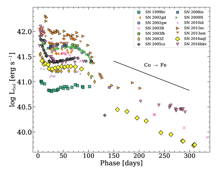
Figure 4: Bolometric light curve of SN 2016aqf compared to our LL SNe II sample. The light curves were obtained by using bolometric corrections (see Section 3.4 for details). All data is corrected for MW and host galaxy extinction (except for those with values reported as upper limits, see Table 3). The ⁵⁶Co $\rightarrow$ ⁵⁶Fe decay line is shown for comparison. Uncertainties are not shown for visualisation purposes

We estimated the bolometric light curve of SN 2016aqf by applying the bolometric correction from Lyman et al. (2014) (assuming a cooling phase of 20 days). We use the ($g-i$) colour as it shows the smallest dispersion. Most SNe in our LL SN II sample have only $BVRI$ data, so, to be consistent, we calculated their bolometric light curves (correcting for MW extinction only) by applying the relation from Lyman et al. (2014) as well, but with ($B-I$) colour as it has the smallest dispersion within the available bands, using the distances from Table 3. Only epochs with simultaneous $B$ and $I$ bands (or $g$ and $i$ for SN 2016aqf) were used. The light curves are shown in Fig. 4 (SN 2008bk is not shown as it does not have epochs with simultaneous $B$ and $I$ coverage). Unfortunately, as the relations from Lyman et al. (2014) only work in a given colour range, we can not estimate the bolometric light curve during the nebular phase of some of the SNe.

The luminosity of SN 2016aqf at peak is $L_{\rm bol}\approx 10^{41.4}$ erg s^-1, estimated from the first epoch with photometry. The luminosity of SN 2016aqf during the cooling phase generally decreases less steeply than other LL SNe II. During the plateau phase, the luminosity falls to $L_{\rm bol}\approx 10^{41.3}$ erg s^-1, placing it in the mid-luminosity range of our sample (between SN 2005cs and SN 2002gd). After the gap, the SN has a luminosity of $L_{\rm bol}$ $\approx$ $10^{40.5}$ erg s^-1, dropping to $L_{\rm bol}$ $\approx$ $10^{39.7}$ erg s^-1 at +300 d. The exponential tail is steeper than ⁵⁶Co decay (0.98 mag per 100 days Woosley et al., 1989), although shallower than the decay in the $V$-band, presumably due to $\gamma$-ray leakage.

3.5 Early spectral evolution

The spectra of SN 2016aqf have narrower lines than spectra of normal SNe II, suggesting low expansion velocities and low explosion energies. Spectra obtained during the optically-thick phase are shown in Fig. 5. During the first two weeks, the evolution is mainly dominated by a blue continuum and Balmer lines, showing P-Cygni profiles of H$\alpha$ and H$\beta$. Fe ii $\lambda 4924$, $\lambda 5018$, $\lambda 5169$ and Ca ii $\lambda\lambda\lambda 8498,8542,8662$ then appear, becoming prominent at later epochs. The Na i D appears at around one month. Sc ii/Fe ii $\lambda 5531$, Sc ii $\lambda 5663$, $\lambda 6247$ and Ba ii $\lambda 6142$ appear at around +50 d. O i $\lambda 7774$ is weakly present after one month.

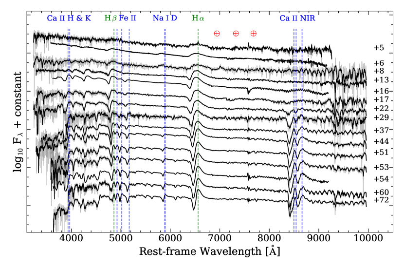
Figure 5: SN 2016aqf photospheric phase spectra. Ca ii H&K, H$\beta$, Fe ii $\lambda\lambda\lambda 4924,5018,5169$, Na i D, H$\alpha$ and Ca ii NIR lines are marked. Green vertical lines denote single lines, while blue denotes doublets or triplets. Telluric lines are shown by red circles with crosses. In some cases, the binned spectra (black line) are over-plotted on the original spectra (grey) for visualisation. Spectra corrected for MW extinction.

Fig. 6 shows the spectra of SN 2016aqf  with other SNe from our comparison sample. The Fe ii lines are present in all SNe, although in SN 2016aqf they are generally weaker. SN 2016aqf is similar to SN 2002gw and SN 2010id, with a relatively featureless spectrum between H$\beta$ and H$\alpha$. However, we see no major differences with the rest of the sample at $\sim$ +15 d.

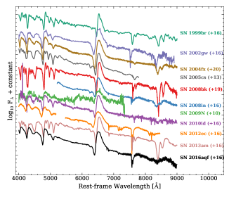
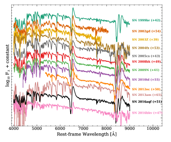
Figure 6: SN 2016aqf spectrum around +15 d (left) and +50 d (right) compared with the LL SNe II sample at similar epochs. Spectra corrected for MW and host galaxy extinction (except for those with values reported as upper limits, see Table 3).

At around +50 d (Fig. 6), SN 2016aqf resembles SN 2009N, with the difference that the Sc ii/Fe ii $\lambda 5531$, Sc ii $\lambda 5663$, $\lambda 6247$ and Ba ii $\lambda 6142$ lines are weaker (and weaker than most other SNe in our sample). O i $\lambda 7774$ is seen in the spectrum of most SNe, except SN 2002gd and SN 2016bkv where the signal-to-noise/resolution of the spectra precludes a secure identification. Most SNe have very similar Fe ii and Ca ii NIR line profiles. SN 2016aqf does not display any other peculiarity with respect to the comparison sample. Note that host galaxy extinction may be substantial for SN 2013am (Zhang et al., 2014; Tomasella et al., 2018), explaining the drop in flux at the bluer end of this SN.

Table 4 shows a list of lines with pseudo-Equivalent Width (pEW, not corrected for instrumental resolution), including the full-width at half maximum (FWHM, not corrected for instrumental resolution) of H$\alpha$, measured from the spectra of SN 2016aqf during the optically-thick phase.

Table 4: pEW for several lines during the optically thick phase and H_α FWHM. These values are not corrected for instrument resolution. Phase with respect to the explosion epoch.

Phase	pEW(Hβ)	pEW(Fe II 4924)	pEW(Fe II 5018)	pEW(Fe II 5169)	pEW(Na I D)	pEW(Ba II 6142)	pEW(Sc II 6247)	pEW(Hα)	FWHM(Hα)
	[Å]	[Å]	[Å]	[Å]	[Å]	[Å]	[Å]	[Å]	[Å]
13	31.7 $\pm$ 3.1	-	-	-	-	-	-	19.0 $\pm$ 0.9	189.7 $\pm$ 2.5
16	34.0 $\pm$ 2.0	-	1.3 $\pm$ 0.1	12.7 $\pm$ 0.4	-	-	-	29.2 $\pm$ 3.2	170.0 $\pm$ 2.6
17	33.9 $\pm$ 0.8	-	-	13.7 $\pm$ 0.4	-	-	-	31.3 $\pm$ 3.1	181.3 $\pm$ 3.5
22	51.0 $\pm$ 2.6	-	16.3 $\pm$ 0.6	19.3 $\pm$ 1.5	-	-	-	46.0 $\pm$ 2.0	156.0 $\pm$ 1.7
29	32.3 $\pm$ 1.5	-	-	-	-	-	-	62.0 $\pm$ 7.0	140.0 $\pm$ 5.2
37	37.7 $\pm$ 1.2	6.3 $\pm$ 0.8	16.2 $\pm$ 0.8	23.7 $\pm$ 7.6	6.9 $\pm$ 1.3	3.2 $\pm$ 0.5	4.1 $\pm$ 1.0	62.3 $\pm$ 4.5	113.0 $\pm$ 6.0
44	43.3 $\pm$ 1.5	8.2 $\pm$ 0.4	19.3 $\pm$ 1.5	31.3 $\pm$ 2.3	9.4 $\pm$ 0.9	5.1 $\pm$ 0.4	3.9 $\pm$ 0.7	65.7 $\pm$ 3.2	100.3 $\pm$ 6.1
51	42.0 $\pm$ 1.0	11.7 $\pm$ 1.1	20.7 $\pm$ 1.2	31.0 $\pm$ 2.0	16.8 $\pm$ 0.3	6.0 $\pm$ 0.6	5.0 $\pm$ 0.5	65.3 $\pm$ 3.5	101.3 $\pm$ 3.8
53	47.3 $\pm$ 2.3	12.8 $\pm$ 0.7	22.0 $\pm$ 1.0	34.0 $\pm$ 1.7	19.7 $\pm$ 2.3	9.6 $\pm$ 1.0	7.8 $\pm$ 1.5	64.0 $\pm$ 2.6	93.7 $\pm$ 3.2
54	55.0 $\pm$ 3.6	11.7 $\pm$ 0.5	20.3 $\pm$ 0.6	33.7 $\pm$ 2.1	24.0 $\pm$ 1.7	8.9 $\pm$ 1.6	5.0 $\pm$ 0.4	68.7 $\pm$ 1.5	94.0 $\pm$ 3.0
60	45.3 $\pm$ 2.9	14.3 $\pm$ 0.5	23.0 $\pm$ 1.0	37.0 $\pm$ 3.0	24.0 $\pm$ 2.6	11.0 $\pm$ 1.1	7.1 $\pm$ 0.3	66.0 $\pm$ 2.6	88.3 $\pm$ 2.5
71	37.0 $\pm$ 1.7	17.7 $\pm$ 0.6	25.0 $\pm$ 1.0	40.3 $\pm$ 1.5	30.7 $\pm$ 2.1	15.3 $\pm$ 1.2	7.2 $\pm$ 0.5	62.0 $\pm$ 2.6	82.7 $\pm$ 5.0

3.6 Nebular spectral evolution

Fig. 7 shows the spectra taken during the optically thin phase. H$\beta$ is present, although its strength slowly decreases at $>250$ d. The Fe ii lines around $5000$ Å are weak and hard to distinguish. The [O i] $\lambda\lambda 6300,6364$ doublet has two distinguishable components (separated by $\sim 62$ Å), and appears after five months, becoming prominent. At five months, we see the presence of He i $\lambda 7065$, [Fe ii] $\lambda 7155$, [Ca ii] $\lambda\lambda 7291,7323$ and [Ni ii] $\lambda 7378$, which become prominent at later epochs. Despite being a LL SN II, SN 2016aqf displays blended [Ca ii] $\lambda\lambda 7291,7323$ lines. The presence of O i $\lambda 7774$ is more prominent at these later epochs. The Ca ii NIR lines are easy to distinguish given the narrow profiles.

The [O i] $\lambda\lambda 6300,6364$ and [Ca ii] $\lambda\lambda 7291,7323$ lines show some very minor redshift ($\sim 5$ Å, or $\sim 230$ km s^-1 and $\sim 200$ km s^-1), while the He i $\lambda 7065$, [Fe ii] $\lambda 7155$ and [Ni ii] $\lambda 7378$ lines are more redshifted ($\sim$ 15 Å, or $\sim 630$ km s^-1, $\sim 630$ km s^-1 and $\sim 610$ km s^-1) throughout most of the nebular phase. We also noticed that the [Ni ii] $\lambda 7378$ line shows almost no redshift ($\sim$ 2 Å, or $\sim 80$ km s^-1) at $\sim$ +150 days before rapidly increasing to $\sim$ 10 Å ($\sim 400$ km s^-1) at $\sim$ +165 days and $\sim$ 20 Å ($\sim 800$ km s^-1) at $\sim$ +270 days. In addition, the [O i] $\lambda\lambda 6300,6364$ lines show a minor blueshift ($\sim$ 5 Å, $\sim 230$ km s^-1) at $\sim$ +280 days and then gets blueshifted again in about one month. These shifts could be caused by asymmetries caused by clumps in different layers of the expanding envelope. It is worth mentioning that the [Fe ii] $\lambda 7172$ and [Ni ii] $\lambda 7412$ lines can contribute to the shifts in the [Fe ii] $\lambda 7155$ and [Ni ii] $\lambda 7378$ lines, respectively. However, due to the resolution of the spectra, we are unable to discern their contribution. Table 5 contains a list of lines and FWHM measurements of SN 2016aqf.

Table 5: FWHM for lines during the optically-thin phase. Values are corrected for the instrument resolution.

Phase	FWHM([O I] 6300)	FWHM([O I] 6364)	FWHM(Hα)	FWHM(He I 7065)	FWHM([Fe II] 7155)
[days]	[Å]	[Å]	[Å]	[Å]	[Å]
155	-	-	43.8 $\pm$ 0.6	47.8 $\pm$ 3.1	41.2 $\pm$ 2.1
168	29.5 $\pm$ 2.1	18.7 $\pm$ 2.1	40.0 $\pm$ 0.6	36.3 $\pm$ 2.6	36.3 $\pm$ 2.0
202	33.6 $\pm$ 1.5	20.8 $\pm$ 2.1	40.5 $\pm$ 0.6	30.3 $\pm$ 1.0	34.3 $\pm$ 1.2
220	38.2 $\pm$ 6.7	23.6 $\pm$ 1.2	38.2 $\pm$ 0.6	32.7 $\pm$ 1.0	34.7 $\pm$ 1.5
259	24.9 $\pm$ 2.5	17.8 $\pm$ 1.2	37.8 $\pm$ 0.6	24.4 $\pm$ 1.5	34.3 $\pm$ 1.5
271	24.4 $\pm$ 2.5	20.8 $\pm$ 2.1	39.4 $\pm$ 0.6	23.0 $\pm$ 1.5	34.7 $\pm$ 1.5
285	27.5 $\pm$ 2.1	20.8 $\pm$ 3.8	35.9 $\pm$ 0.6	28.7 $\pm$ 1.5	32.4 $\pm$ 1.2
303	28.2 $\pm$ 2.5	22.2 $\pm$ 4.0	35.4 $\pm$ 0.6	27.0 $\pm$ 0.6	29.5 $\pm$ 1.5
330	28.2 $\pm$ 1.5	24.9 $\pm$ 2.1	35.9 $\pm$ 0.6	28.2 $\pm$ 2.1	34.7 $\pm$ 1.2
351	39.7 $\pm$ 3.6	19.8 $\pm$ 4.4	37.8 $\pm$ 0.6	70.9 $\pm$ 9.0	43.4 $\pm$ 4.0

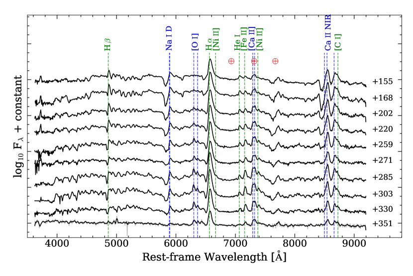
Figure 7: SN 2016aqf nebular phase spectroscopy. H $\alpha$, H $\beta$, Na i D, [O i] $\lambda\lambda 6300,6364$, [Ni ii] $\lambda 6667$, He i $\lambda 7065$, [Fe ii] $\lambda 7155$, [Ca ii] $\lambda\lambda 7291,7323$, [Ni ii] $\lambda 7378$ and Ca ii NIR lines are shown for guidance. The rest of the description is the same as in Fig. 5.

When we compare SN 2016aqf to other SNe at $>+300$ d (see Fig. 8), some of them do not show He i $\lambda 7065$ (e.g., SN 2005cs and SN 2012ec). For SN 2009N, which does show this line, it has a similar strength to [Fe ii] $\lambda 7155$, which does not occur for other SNe. The ratio between the [O i] $\lambda\lambda$6300, 6364 lines are similar for all SNe, except for SN 2005cs where these lines have a similar flux. It can also be seen that [Ni ii] $\lambda 7378$ is easy to distinguish in some SNe (e.g., SN 2012ec, SN 2009N and SN 2016aqf). In the case of SN 2003B and SN 2005cs, this line is present, but it gets blended with the [Ca ii] $\lambda\lambda 7291,7323$ doublet. SN 2012ec is a special case as it is the only SN that shows a higher peak in [Ni ii] $\lambda 7378$ than in the [Ca ii] $\lambda\lambda 7291,7323$ doublet.

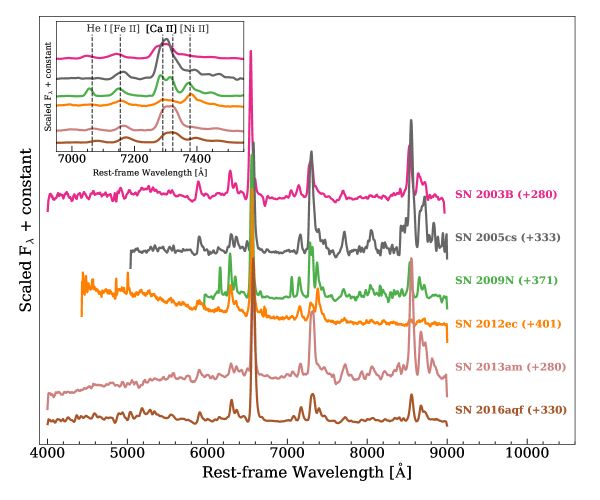
Figure 8: SN 2016aqf spectrum around +330 d compared with the LL SN II sample at similar epochs. The spectra were normalised by their peak H$\alpha$ flux. Embedded figure: zoom-in around $\sim 7250$ Å. The rest-frame position of the He i $\lambda 7065$, [Fe ii] $\lambda 7155$, [Ca ii] $\lambda\lambda 7291,7323$ and [Ni ii] $\lambda 7378$ lines are shown. Spectra corrected for MW host galaxy extinction (except for those with values reported as upper limits, see Table 3).

3.7 Expansion velocity evolution

The ejecta expansion velocities were measured from the position of the absorption minima for H$\beta$, Fe ii $\lambda 4924$, Fe ii $\lambda 5018$, Fe ii $\lambda 5169$, Na i D (middle of the doublet), Ba ii $\lambda 6142$, Sc ii $\lambda 6247$ and H$\alpha$. For H$\alpha$, we also estimated the expansion velocity from the FWHM (corrected for the instrumental resolution) of the emission by using $v=c\times\mathrm{FWHM}/\lambda_{\rm rest}$, where $c$ is the speed of light. We include uncertainties in the measurement of the absorption minima, from the host galaxy recession velocity (3 km s^-1, as reported in HyperLEDA; Makarov et al. 2014), the maximum rotation velocity of the galaxy (44.2 km s^-1, as reported in HyperLEDA) and from the instrumental resolution, all added in quadrature. The major contribution to the uncertainty comes from the instrumental resolution.

The expansion velocity curves are shown in Fig. 9. The velocities of H$\alpha$ and H$\beta$ are relatively high ($\gtrsim 8000$ km s^-1) at very early epochs ($t\lesssim 10$ days) and drop to $\sim 5000$ and $4000$ km s^-1 at $\sim 50$ days, respectively, decreasing at a slower rate afterwards. The H$\alpha$ velocity estimated from the FWHM is close to that estimated from the absorption minima as shown by Gutiérrez et al. (2017). The velocities of other lines decrease less dramatically, from $\sim 5000$ km s^-1 at early epochs ($t\sim$ 10 d), for the Fe ii lines, dropping down to $\sim 3000$ km s^-1 at $\sim$ 50 d, and then constant thereafter.

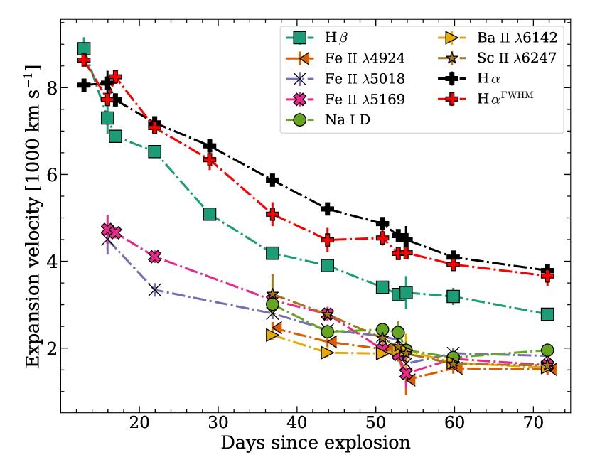
Figure 9: SN 2016aqf expansion velocities for H $\beta$, Fe ii $\lambda 4924$, Fe ii $\lambda 5018$, Fe ii $\lambda 5169$, Na i D (middle of the doublet), Ba ii $\lambda 6142$, Sc ii $\lambda 6247$ and H $\alpha$. For H $\alpha$ we also estimated the expansion velocity from the FWHM; see text for details.

In general, the expansion velocity curves of SN 2016aqf fall within the bulk of our sample and follow the general trend, although some of the velocities seem to decrease faster during the first 50 days after explosion.

4 Physical Parameters

4.1 Nickel Mass

The M_Ni is one of the main physical parameters that characterise CCSNe as it is formed very close to the core (within a few thousand kilometers; e.g., Kasen & Woosley 2009). We estimated the nickel mass of SN 2016aqf by using different methods. These come from: (i) Arnett (1996), (ii) Hamuy (2003), (iii) Maguire et al. (2012) and (iv) Jerkstrand et al. (2012). For more information regarding the different relations used for the estimation of the nickel mass, see Appendix A.

For (i), (ii) and (iv), we used the bolometric luminosity of the exponential decay tail at +200 days, calculated in Sec. 3.4 by interpolating with Gaussian Process (Rasmussen & Williams, 2006), using the python package george (Ambikasaran et al., 2015) and including the distance of the SN for (ii). In the case of (iii), we measured the FWHM of $H_{\alpha}$ at +351 days, correcting it for the FWHM of the instrument. The M_Ni values obtained with the different methods were M_Ni = $0.008^{+0.002}_{-0.002}$, $0.011^{+0.003}_{-0.003}$, $0.014^{+0.009}_{-0.007}$ and $0.007^{+0.001}_{-0.001}$ M_⊙, respectively. Using the different methods we estimated a weighted mean and a weighted standard error of the mean of M${}_{\rm Ni}=0.008\pm 0.002$ M_☉.

4.2 Explosion Energy, Ejected Mass and Progenitor Radius

Popov (1993) derived analytical relations for the estimation of the explosion energy ($\mathrm{E}_{\mathrm{exp}}$), ejected envelope mass ($\mathrm{M}_{\mathrm{env}}$) and the progenitor radius prior to outburst ($\mathrm{R}_{\mathrm{prog}}$) for SNe II-P (following a similar analysis by Litvinova & Nadezhin 1985). These parameters are related to different light-curve properties and also M_Ni, therefore, they are essential for the characterisation of SNe II and CCSNe in general. The relations found by Popov (1993) are

$$\log_{10}(\mathrm{E}_{\mathrm{exp}})=4.0~{}\log_{10}~{}t_{\text{p}}+0.4~{}M_{V}+5.0~{}\log_{10}(v_{\text{ph}})-4.311,$$ (1)

$$\log_{10}(\mathrm{M}_{\mathrm{env}})=4.0~{}\log_{10}~{}t_{\text{p}}+0.4~{}M_{V}+3.0~{}\log_{10}(v_{\text{ph}})-2.089,$$ (2)

and

$$\log_{10}(\mathrm{R}_{\mathrm{prog}})=-2.0~{}\log_{10}~{}t_{\text{p}}-0.8~{}M_{V}-4.0~{}\log_{10}(v_{\text{ph}})-4.278,$$ (3)

where $M_{V}$ is the $V$-band absolute magnitude at the middle of the plateau, $t_{\rm p}$ is the duration of the plateau in days (as in Hamuy 2003), $v_{\rm ph}$ is the expansion velocity of the photosphere at $t_{\rm p}/2$ (usually measured from the Fe ii $\lambda 5169$ line, as it has shown to be a good tracer of the photosphere) in $10^{3}$ km s^-1. $\mathrm{E}_{\mathrm{exp}}$ is expressed in $10^{51}$ erg, and $\mathrm{M}_{\mathrm{env}}$ and $\mathrm{R}_{\mathrm{prog}}$ in solar units. We measured M${}_{V}=-14.63\pm 0.27$ mag for which we used Gaussian processes to interpolate the light curve. By using the relativistic Doppler shift, we obtained $v_{\rm ph}=2068\pm 167$ km s^-1 from the Fe ii $\lambda 5169$ absorption line minima. Finally, we use $t_{\rm p}=97.9\pm 7.2$ days, for which we assumed the same value of SN 2003fb, adding its uncertainty (see Anderson et al., 2014) in quadrature, as these SNe have relatively similar evolution around the transition ($t\gtrsim$ +50 days) in the $V$ band (see Appendix B). With these values for SN 2016aqf we obtained $\mathrm{E}_{\mathrm{exp}}$ $=0.24~{}\pm~{}0.13~{}\times 10^{51}$ erg, $\mathrm{M}_{\mathrm{env}}$ $=9.31~{}\pm~{}4.26$ M_☉ and $\mathrm{R}_{\mathrm{prog}}$ $=152~{}\pm~{}94~{}\text{R}_{\odot}$. The large uncertainties come mainly from the velocity, specifically from the instrumental resolution, and from the distance uncertainty used in calculating the absolute magnitude. We compared these results with similar relations found in the literature (e.g., Kasen & Woosley, 2009; Shussman et al., 2016; Sukhbold et al., 2016; Kozyreva et al., 2019; Goldberg et al., 2019; Kozyreva et al., 2020), obtaining similar results.

SN 2016aqf follows the $\mathrm{E}_{\mathrm{exp}}$$-$M_Ni relation found in SNe II (e.g., Pejcha & Prieto, 2015; Müller et al., 2017), and $\mathrm{M}_{\mathrm{env}}$ follows the $\mathrm{M}_{\mathrm{env}}$$-$$\mathrm{E}_{\mathrm{exp}}$ relation (e.g., Pejcha & Prieto, 2015). If we assume a neutron star ($\sim 1.4$ M_☉) as the compact remnant, the progenitor of SN 2016aqf should be a RSG with $\sim 10.7$ M_☉. This is a lower limit, as some mass loss is expected due to various processes, e.g., winds (e.g. Dessart et al., 2013b). Finally, $\mathrm{R}_{\mathrm{prog}}$ is well within the normal values of RSG radii, although on the lower end (e.g., Pejcha & Prieto, 2015; Müller et al., 2017), but consistent with other estimations for this sub-class of SN (e.g., Chugai & Utrobin, 2000; Zampieri et al., 2003; Pastorello et al., 2009; Roy et al., 2011).

5 Discussion

5.1 Progenitor Mass

The progenitors of SNe II have been extensively studied through pre-SN images (e.g. Smartt et al., 2009; Smartt, 2015) and hydrodynamical models (e.g. Bersten et al., 2011; Dessart et al., 2013b; Martinez & Bersten, 2019). Although there remain some disagreements (e.g., Utrobin & Chugai, 2009; Dessart et al., 2013b, for discussions of this discrepancy), there have been recent major improvements due to better cadence observations.

The [O i] $\lambda\lambda 6300,6364$ nebular-phase lines have also been shown to be good tracers of the core mass of CCSN progenitors (e.g., Elmhamdi et al., 2003; Sahu et al., 2006; Maguire et al., 2010), as at these later epochs we are observing deeper into the progenitor structure. Spectral modelling of the nebular phase has shown good agreement with this and can be used to estimate the progenitor mass (e.g., ; ; , ). In order to estimate the progenitor mass of SN 2016aqf, we used the spectral synthesis models from J14 and J18 for progenitors with three different ZAMS masses: 9, 12 and 15 M_☉. The 9 M_☉ model has an initial ⁵⁶Ni mass of $0.0062$ M_☉ while the other two models have an initial ⁵⁶Ni mass of 0.062 M_☉. We compare the nebular spectra of SN 2016aqf with the models at two different epochs each (see Fig. 10 for models at +300 days). The models are scaled by exp((t_mod - t_SN)/111.4), where t_mod is the epoch of the spectrum of the models and t_SN is the epoch of the spectrum of the SN, by the SN nickel mass, M${}_{\rm Ni}^{\rm SN}$/M${}_{\rm Ni}^{\rm mod}$, and by the inverse square of the SN distance, (d_mod/d_SN)². The luminosity of some lines, like [O i] $\lambda 6300,6364$, scale relatively linearly with the M_Ni (as discussed, e.g., in J14), thus, it is reasonably accurate to compare the models rescaled, with the difference in M_Ni, to our observed SN. $\chi^{2}$ values are calculated to quantify these comparisons as well.

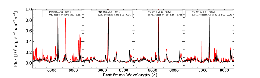
Figure 10: First three panels (from left to right): Spectral synthesis models of SNe II from J14 and J18. Three spectral synthesis models at $\sim$+300 d from different progenitor masses: 9 (left panel), 12 (centre) and 15 M_☉ (right). $X$ is the scaling factor (see Sec. 5.1). The 12 and 15 M_☉ models fit the spectrum better than the 9 M_☉model, including the [O i] $\lambda\lambda 6300,6364$ lines. Last panel: YN2 model of 12 M_☉ from Lisakov et al. (2017). There is a relatively good agreement with some of the Ca and the [O i] $\lambda 6300,6364$ lines, however, most other lines are over-predicted.

From Fig. 10 we see that the 12 and 15 M_⊙ models present similar results, reproducing several lines. They can partially reproduce the [O i] $\lambda 6300$ line, but the latter does not reproduce the [O i] $\lambda 6364$ line very well. However, these models under-predict the [Fe ii] $\lambda 7155$ line and do not reproduce the [Ni ii] $\lambda 7378$ line and Ca ii NIR triplet. The 9 M_☉ mostly over-predicts the flux of lines, but does a good job reproducing the He i $\lambda 7065$ and [Fe ii] $\lambda 7155$ lines. In terms of $\chi^{2}$ values, the 12 M_☉ model is slightly better than the 15 M_☉ one, while the 9 M_⊙ model has a poorer fit. In addition, the 12 M_⊙ model is relatively consistent with the mass estimate from Sec. 4.2, within the uncertainty. We also measured [O i]/[Ca ii] flux ratios (e.g., Maguire et al., 2010) between $\sim 0.5$–$0.7$, which are consistent with the 12 M_☉ model and roughly consistent with the 15 M_☉ model. Finally, we found that the models reproduce lines better at later epochs ($\gtrsim 300$ d) than at early epochs ($<300$ d). J18 found the same pattern.

There seems to be a very weak detection of [Ni ii] $\lambda 6667$ (see Fig. 7), partially blended with H $\alpha$, and the 9 M_☉ model predicts similar fluxes for this line and [Ni ii] $\lambda 7378$, due to the high optical depths (fig. 20 of J18). Note that this model has only primordial nickel in the hydrogen-zone, no synthesised ⁵⁸Ni, and a different setup compared to the other two (e.g., no mixing applied, J18, ). As the model prediction for [Ni ii] $\lambda 7378$ is too weak, one can argue the detection of synthesised nickel. The 9 M_☉ model over-predicts the [O i] $\lambda 6300,6364$ lines, including most other lines. As mentioned above, J18 had similar results at these early epochs, however, this model showed better agreement at later epochs (e.g., $>350$ d for SN 2005cs). We did not find better agreement at later epochs.

In order to expand our analysis we also compared SN 2016aqf with the progenitor models from Lisakov et al. (2017), specifically, the YN models of 12 M_☉ (a set of piston-driven explosion with ⁵⁶Ni mixing) as their M_Ni (0.01 M_☉) agree perfectly with our estimation, apart from agreeing with other physical parameters (e.g., $\mathrm{E}_{\mathrm{exp}}$ = $2.5\times 10^{50}$ erg, $\mathrm{M}_{\mathrm{env}}$ = 9.45 M_☉) as well. This comparison, which was done in the same way as with the other models above, is shown in Fig. 10 for the YN2 model as well. As can be seen, the model predicts some of the Ca and the [O i] $\lambda 6300,6364$ lines relatively well. Nonetheless, most of the other lines are over-predicted. Other models from Lisakov et al. (2017) did not show better agreement. However, the fact that both 12 M_☉ models (from J14 and Lisakov et al. 2017) partially agree with the [O i] $\lambda 6300,6364$ lines (the main tracers of the ZAMS mass) strengthen the conclusion that the progenitor is probably a $\sim$ 12 M_☉ RSG star.

We would like to emphasise that neither the 9 M_☉ model from J18 nor the YN 12 M_☉ models from Lisakov et al. (2017) have macroscopic mixing. The consistent overproduction of narrow core lines in both models (see Figs. 10 and LABEL:fig:cmfgen_model) suggests that mixing is necessary, which the models from J14 have.

In conclusion, this shows that the current models have problems predicting the observed diversity of LL SNe II, probably due to the incomplete physics behind these explosions (e.g., assumptions of mixing, ⁵⁶Ni mass, rotation). In other words, there is a need of more models with different parameters that can help to understand the observed behaviour of these SNe. As such, we can not exclude a 9 M_☉ nor a 15 M_☉ progenitor. Thus, we conclude that the progenitor of SN 2016aqf had a ZAMS mass of 12 $\pm$ 3 M_☉. A more detailed modelling of the progenitor is needed to improve these constrains, although this is beyond the scope of this work.

5.2 He ${\rm I}$ $\lambda 7065$

The He i $\lambda 7065$ nebular line has been studied with theoretical modelling (e.g., Dessart et al. 2013a; J18), giving a diagnostic of the He shell. These models predict the appearance of this line in SNe II with low mass progenitors as more massive stars have more extended oxygen shell, shielding the He shell from gamma-ray deposition. However, some LL SNe II do not show this line in their spectra (e.g., SN 2005cs; see Fig. 8). SN 2016aqf shows the clear presence of He i $\lambda 7065$ throughout the entire nebular coverage. We also see the presence of [C i] $\lambda 8727$, although it gets partially blended with the Ca ii NIR triplet. We expect to see this carbon line as a result of the He shell burning, so the presence of both lines (He i $\lambda 7065$ and [C i] $\lambda 8727$) is consistent with the theoretical prediction. Thus, we believe that SN 2016aqf is a good case study to provide further understanding of the He shell zone through theoretical models. Furthermore, following the discussion from J18, we conclude that this is a Fe core SN and not an electron-capture SN (ECSN), as the latter lack lines produced in the He layer.

5.3 Ni/Fe abundance ratio

As discussed above, the nebular spectra of SNe II contain a lot of information regarding the progenitors as we are looking deeper into its structure. J15a discussed the importance of the ratio between the [Ni ii] $\lambda 7378$ and [Fe ii] $\lambda 7155$ lines as indicator of the Ni/Fe abundance ratio. These elements are synthesised very close to the progenitor core and, for this reason, their abundances get affected by the inner structure of the progenitor and the explosion dynamics. More specifically, iron-group yields are directly affected mainly by three properties: temperature, density and neutron excess of the fuel (for a more detailed account, see J15b, ). For this reason, studying iron-group abundances is key to understanding SNe II.

SN 2016aqf is the only SN II to date with a relatively extensive coverage of the evolution of [Ni ii] $\lambda 7378$ (most other SNe with the presence of this line only have at most $\sim$ 2 epochs showing it). In Fig. 11 we show the evolution in time of the flux of [Ni ii] $\lambda 7378$ and [Fe ii] $\lambda 7155$, and their luminosity ratio. We estimated the fluxes by fitting Gaussians to the profiles. Uncertainties were estimated by repeating the measurements and assuming different continuum levels, but we do not include the uncertainty coming from the instrumental resolution in any of the measured fluxes throughout this work. However, this should not greatly affect the measurements as the spectral lines are in general much wider than the instrumental resolution (e.g., [Fe ii] $\lambda 7155$ has an average FWHM of $\sim$ 35 Å).

We notice that the evolution of the luminosity ratio reaches a quasi-constant value after $\sim$ 170 days since the explosion. This suggests that at relatively late nebular phase the Ni/Fe abundance ratio is constant as the temperature should not vary much (see J15a, ), although clumps in the ejecta might cause deviations from the measured values. After removing the value at $\sim$ +155 days (as the SN might still be in the transition to the optically thin phase) we report a Ni/Fe luminosity ratio weighted mean of $0.906$ and a standard deviation of $0.062$. The standard deviation gives us a more conservative estimation of the uncertainty in the Ni/Fe luminosity ratio than the uncertainty in the weighted mean.

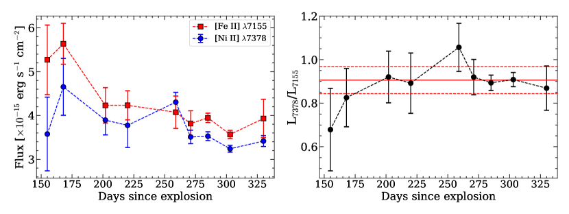
Figure 11: Left panel:[Ni ii] $\lambda 7378$ and [Fe ii] $\lambda 7155$ lines fluxes. Right panel: Luminosity ratio of these lines. The weighted average (solid red line) with a one standard deviation (dashed red lines) are shown for guidance. The value at $\sim$ +150 days was removed for these calculations.

We follow J15a to estimate the Ni ii/Fe ii ratio and in turn the Ni/Fe abundance ratio. From the ratio between the luminosity of the [Fe ii] $\lambda 7155$ line and M_Ni, we then obtained a temperature constrain of $T=3919^{+215}_{-257}$ K. With these values we estimated the Ni/Fe abundance ratio to be $0.081^{+0.009}_{-0.010}$, or $\sim$ 1.4 times the solar ratio ($0.056$, Lodders 2003).

However, there are several things we need to take into consideration. Contribution to the [Fe ii] $\lambda 7155$ and [Ni ii] $\lambda 7378$ lines does not come only from synthesised material, but also from primordial Fe and Ni in the H-zone (J15a). The contribution can be significant ($\sim$ 40 per cent) and depends on the model and epoch. Unfortunately, the effect of primordial contamination is not easy to remove without detailed theoretical modelling. Nonetheless, it is plausible that the [Fe ii] $\lambda 7155$ and [Ni ii] $\lambda 7378$ lines are greatly dominated by synthesised Fe and Ni at relatively early epochs ($\lesssim 300$ d), although we are uncertain at which epochs the effect from primordial Fe and Ni starts becoming important (J18). The line ratio can also be affected at very early epochs ($\lesssim 200$ d), as the SN can still be during the optically-thick phase when opacity plays an important role.

Few other SNe have been reported to show [Ni ii] $\lambda 7378$. It is possible that this line is mainly visible in LL SNe II, where the expansion velocities are lower, producing narrower deblended line profiles. However, it is also seen in non-LL SNe II, other CCSNe (e.g., SN 2006aj; Maeda et al., 2007; Mazzali et al., 2007) and type Ia SNe (SNe Ia; e.g. Maeda et al., 2010). We searched for objects in our LL SN II comparison sample with spectra in which we could detect [Fe ii] $\lambda 7155$ and [Ni ii] $\lambda 7378$ to measure the Ni/Fe abundance ratio as for SN 2016aqf. We also expanded this sample to include other LL SNe II: SN 1997D, SN 2003B, SN 2005cs, SN 2008bk, SN 2009N and SN 2013am.

SN 1997D and SN 2008bk were not included in our initial sample as they lack good publicly available data. We also include SN 2012ec as it is a well-studied case. In the case of SN 1997D, we measured the ratio at two different epochs, but we used one (at $\sim$ +384 days) of those, given that the other value (at $\sim$ +250 days) had relatively large uncertainties. For SN 2009N we took an average between the two values (at $\sim$ +372 and +412 days) we were able to measure as they were relatively similar. SN 2016bkv was not included as the M_Ni values obtained in Nakaoka et al. (2018) and Hosseinzadeh et al. (2018) for this SN are not consistent with each other ($\sim$ 0.01 M_☉ and 0.0216 M_☉, respectively), this being necessary for an accurate estimation of the Ni/Fe abundance ratio. For the rest of the SNe, only one value was obtained. Several other LL SNe II show the presence of [Ni ii] $\lambda$7378, but it is either blended with other lines or the SNe lack some of the parameters needed to estimate the Ni/Fe abundance ratio.

To expand our analysis we looked into other physical parameters related to the Ni/Fe abundance ratio. For example, J15b further analyse and compare this ratio against theoretical models. Some of these models show that at lower progenitor mass, the Ni/Fe abundance ratio should be higher. We investigate this by increasing our sample. Unfortunately not many LL SNe II have measured progenitor masses from pre-SN images, so we added non-LL SNe II as several of these do (e.g., Smartt, 2015), while they also show the presence of [Fe ii] $\lambda 7155$ and [Ni ii] $\lambda 7378$ in their spectra. We do not include SNe with estimates of the progenitor mass from other methods as they depend on more assumptions than the pre-SN images method, making these estimates less reliable. The SNe included are: SN 2007aa (Anderson et al., 2014; Gutiérrez et al., 2017), SN 2012A (Tomasella et al., 2013) and SN 2012aw (Fraser et al., 2012). All these SNe are included in Table 3. For SN 2007aa we calculated the ejected nickel mass to be M_Ni = 0.032 $\pm$ 0.009 M_☉ (we estimated this value using the relation from Hamuy 2003 and other values from Anderson et al. 2014) and estimated the Ni/Fe abundance ratio also as part of this work. For the other two SNe II, we took the values from J15a, assuming upper and lower uncertainties equal to the average of the uncertainties of the rest of the sample (not taking into account the uncertainties of SN 2012ec as they are too high). The Ni/Fe abundance ratio values for this sample are shown in Table 6.

Table 6: Ni/Fe abundance ratio values used in this work.

SN	Ni/Fe	$\sigma_{-}$	$\sigma_{+}$
SN1997D	0.079	0.025	0.014
SN2003B	0.057	0.021	0.018
SN2005cs	0.084	0.012	0.012
SN2007aa	0.074	0.006	0.006
SN2008bk	0.046	0.042	0.017
SN2009N	0.101	0.018	0.017
SN2012A	0.028	0.022	0.016
SN2012aw	0.084	0.022	0.016
SN2012ec	0.2	0.07	0.07
SN2013am	0.108	0.017	0.018
SN2016aqf	0.081	0.010	0.009

In addition, we compared the Ni/Fe against other physical, light-curve and spectral parameters to investigate possible correlations. The motivation is two-fold. Firstly, we are searching for correlations that might allow indirect methods of measuring this ratio for SNe with blended lines. Secondly, these correlations could shed light on the effect of different parameters in the observed value of Ni/Fe, as is expected for the progenitor mass, important for the theoretical modelling of SNe II.

We examined various parameters we thought could be somehow connected to the Ni/Fe abundance ratio. The most relevant parameters are: nickel mass (M_Ni); SN $V$-band maximum absolute magnitude ($M_{\rm max}^{V}$); optically-thick phase duration (OPT_d); Fe ii $\lambda 5169$ expansion velocity (vel(Fe ii 5169)); the progenitor mass from KEPLER (K) models (M${}_{\rm prog}^{\rm K}$; see Smartt 2015), progenitor mass from STARS and Geneva (SG) rotating models (M${}_{\rm prog}^{\rm SG}$; see Smartt 2015); explosion energy ($E_{\rm exp}$); [O i] $\lambda 6300$ and [O i] $\lambda 6364$ luminosities at the epoch of measured Ni/Fe abundance ratio ($L_{6300}$ and $L_{6364}$); and host galaxy gas-phase metallicity ((12 + log(O/H))_N2). The Ni/Fe abundance ratio versus M_Ni, M${}_{\rm max}^{V}$ and M_prog are shown in Fig. 12.

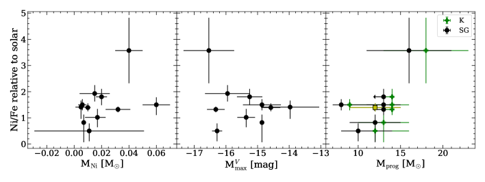
Figure 12: Ni/Fe abundance ratio versus M_Ni, M${}_{\rm max}^{V}$ and M_prog. For M_prog we show two different progenitor models, KEPLER (K) and STARS and Geneva (SG). SN 2016aqf is shown as a yellow square in the subplot with M_prog, for which we assume a value of $12\pm 3$ M_☉.

Pearson and Spearman’s rank correlations were used to investigate if there is any meaningful correlation between these parameters and the Ni/Fe abundance ratio. To account for the measurement uncertainties, we use a Monte Carlo method, assuming Gaussian distributions for symmetric uncertainties, skewed Gaussian distributions for asymmetric uncertainties, and a uniform distribution (with a lower limit of 8 M_☉) for upper limits in the progenitor masses.

We found no significant correlation between the parameters tested above. However, we note that the uncertainties in some parameters are significant. If we do not take into account the uncertainties we obtain a weak correlation between Ni/Fe and M${}_{\rm max}^{V}$ and progenitor mass. However, these are mainly driven by one object (SN 2012ec).

This null result raises some interesting questions. We did not find a correlation between M_Ni and Ni/Fe abundance ratio, which is expected as one would assume the production of ⁵⁶Ni to track the production of ⁵⁸Ni and ⁵⁴Fe (e.g., J15b, ). We expected to see an anti-correlation between progenitor mass and Ni/Fe abundance ratio, as theory predicts that lower-mass stars have relatively thick silicon shells that more easily encompass the mass cut that separates the ejecta from the compact remnant, ejecting part of their silicon layers, which produces higher Ni/Fe abundance ratios. This is supported by the models from Woosley & Weaver (1995) and Thielemann et al. (1996), but not by those of Limongi & Chieffi (2003) which use thermal bomb explosions instead of pistons, as the former two do (see J15b). Having this in mind, our results either indicate that this anti-correlation can be driven by the exact choice of explosion mechanism (e.g., piston-driven explosions, neutrino mechanism, thermal bomb) and physical parameters (e.g., mass cut, composition, density profile), or that low-mass stars typically do not burn and eject Si shells, but either O shells or possibly merged O-Si shells (e.g., Collins et al., 2018). This is an important constraint both for pre-SN modelling (shell mergers and convection physics that determines whether these Si shells are thin or thick) and explosion theory (which matter falls into NS and which is ejected). Finally, we also need to consider the possibility of having primordial Ni and Fe contaminating the measured Ni/Fe abundance ratio, which could affect our results (as discussed above).

As mentioned in J15b, 1D models tend to burn and eject either Si shell or O shell material that gives Ni/Fe abundance ratios of $\sim$ 3 and $\sim$ 1 times solar, respectively. Therefore, there is a clear-cut prediction that we should see a bimodal distribution of this ratio, with relatively few cases where the burning covers both shells. However, the observed distribution of our sample seems to cover the whole $\sim$ 1–3 range. This may suggest that the 1D picture of progenitors is too simplistic. Recent work on multi-D progenitor simulations (e.g., Müller et al. 2016; Collins et al. 2018; Yadav et al. 2020, and references therein), where some of these suggest vigorous convection and shell mixing inside the progenitor. If this happens, Si and O shells could smear together and burning such a mixture would give rise to Ni/Fe abundance ratios covering the observed range depending on the relative masses of the two components.

6 Conclusions

Theoretical modelling has shown that the Ni/Fe abundance ratio, which can be estimated from the [Ni ii] $\lambda 7378$/[Fe ii] $\lambda 7155$ lines ratio, gives an insight of the inner structure of progenitors and explosion mechanism dynamics. To date, very few SNe II have shown these lines in their spectra, most of them been LL SNe II. This could be due to their lower explosion energies (hence lower expansion velocities) which facilitates the deblending of lines, although these lines have also been found in one SN Ic and SNe Ia.

SN 2016aqf has a similar spectral evolution to other SNe of this faint sub-class and has a bolometric luminosity and expansion velocities that follow the bulk behaviour of LL SNe II. When comparing its nebular spectra to spectral synthesis models to constrain the progenitor mass through the [O i] $\lambda\lambda 6300,6364$ lines, we find a relatively good agreement with progenitors of 12 (using two model grids) and 15 M_☉. However, due to uncertainties (e.g., mixing) in the other models, we cannot exclude lower mass ($\sim$ 9 M_☉) progenitors. In addition, we noted that the lack of macroscopic mixing seen in some models produce too much fine structure in the early nebular spectra, which would need to be considered in future modelling. Hence, we conclude that the progenitor of SN 2016aqf had a ZAMS mass of 12 $\pm$ 3 M_☉. To further constraint the progenitor mass a more detailed modelling would be required, although this is outside the scope of this work.

As observed from the theoretical modelling of SNe II progenitors, the presence of He i $\lambda 7065$ and [C i] $\lambda 8727$ in the spectra is linked to the (at least partial) burning of the He shell, which would suggest that SN 2016aqf is a Fe-core SN instead of an ECSN.

SN 2016aqf is a unique case as it has an extended spectral coverage showing the evolution of [Ni ii] $\lambda 7378$ and [Fe ii] $\lambda 7155$ lines for over 150 days. The ratio between these lines appears to be relatively constant (at $t\gtrsim$ +170 days), which would suggest that one spectrum at a relatively late epoch would be enough to measure this quantity. An optimal epoch range to measure this ratio is $\sim$ 200–300 days, given that at earlier epochs the SN can still be in the optically-thick phase when the high opacity blocks the contribution from the lines, and at later epochs the contribution from primordial Fe and Ni is more important. This could vary from SN to SN, so a larger sample with extensive coverage of the [Ni ii] $\lambda 7378$ and [Fe ii] $\lambda 7155$ lines is required. When comparing to a sample of SNe II (LL and non-LL included) with measured Ni/Fe abundance ratio, the SN 2016aqf value falls within the middle of the distribution.

We did not find any anti-correlation between ZAMS mass and Ni/Fe abundance ratio as predicted by theory. We believe this could mean one of two things. On the one hand, as some models predict this anti-correlation, but others do not, this trend could be driven by the choice of explosion mechanism (e.g., piston-driven explosions, neutrino mechanism, thermal bomb) and physical parameters (e.g., mass cut, composition, density profile). On the other hand, this could mean that low-mass stars typically do not burn and eject Si shells, but instead O shells or possibly merged O-Si shells which would alter the produced Ni/Fe abundance ratio. However, one must keep in mind that there is the possibility of having contamination of primordial Ni and Fe, which can be significant (up to $\sim$ 40 per cent) and epoch dependent.

The current picture of 1D progenitors may be too simplistic, as higher dimensional effects, like mixing and convection, can play an important role, which could help reproduce the observed distribution of Ni/Fe abundance ratio.

Finally, we note that nebular-phase spectral coverage of SNe II is essential for the study of these objects. While there exist a number of SN II nebular spectra in the literature, additional higher cadence and higher signal-to-noise observations are required to help improve theoretical models.

Appendix A Nickel Mass estimation

In the literature there are various methods to estimate the ⁵⁶Ni mass. These are as follows.

Arnett (1996) gives the following relation using SN 1987A as comparison:

$$M_{\rm Ni}=0.075\times\frac{L_{\text{SN}}}{L_{\text{87A}}}\text{M}_{\odot}$$ (4)

By using the bolometric light curve calculated in Section 3.4, interpolating with Gaussian Processes to obtain the luminosity at 200 days after the explosion, we obtain $M_{\rm Ni}=0.008\pm 0.001$ M_☉.

Hamuy (2003) formed a relation between the bolometric luminosity of the exponential decay tail and the ⁵⁶Ni  mass. The bolometric luminosity is then given by:

$$\begin{split}log_{10}~{}&L_{\rm tail}=\\ &\frac{-[m_{V,\text{tail}}-A_{\text{MW}}(V)-A_{\text{Host}}(V)+BC]+5~{}log_{10}(D)-8.14}{2.5}\end{split}$$ (5)

where $L_{\mathrm{tail}}$ is the tail luminosity in erg s^-1 at 200 days after the explosion, $D$ is the distance in cm, $BC$ is a bolometric correction that permits one to transform V magnitudes into bolometric magnitudes, and the additive constant provides the conversion from Vega magnitudes into cgs units. From SN 1987A and SN 1999em Hamuy (2001) found that $BC=0.26\pm 0.06$. Using the relation found by Hamuy (2003) the nickel mass is obtained as follows:

$$M_{\rm Ni}=(7.866\times 10^{-44})~{}L_{\text{tail}}~{}exp\Big{[}\frac{(t_{\text{tail}}-t_{0})/(1+z)-6.1}{111.26}\Big{]}\text{M}_{\odot}$$ (6)

from which we obtain $M_{\rm Ni}=0.011\pm 0.003$ M_☉.

Maguire et al. (2012) found a relation between the nickel mass and the H$\alpha$ FWHM given by

$$M_{\rm Ni}=A\times 10^{B\times FWHM_{\text{corr}}}\text{M}_{\odot}$$ (7)

where $B=0.0233\pm 0.0041$, $A=1.81^{+1.05}_{-0.68}\times 10^{-3}$ and FWHM_corr is the FWHM of H_α, corrected by the spectral resolution of the instrument, during the nebular phase ($\sim 350-550$ days). From this relation, using the FWHM of H $\alpha$ from the spectrum at +348 days, we obtain $M_{\rm Ni}=0.014^{+0.009}_{-0.007}$ M_☉, where we used FWHM_inst = 21.2 Å, taken from grism #13 in EFOSC2 (as given in the ESO website).

J12 also gives a relation to estimate the nickel mass from the early exponential-decay tail, assuming full trapping, that the deposited energy is instantaneously re-emitted and that no other energy source has any influence, i.e.,

$$L_{{}^{56}\text{Co}}(t)=9.92\times 10^{41}\frac{M_{\text{Ni}}}{0.07M_{\odot}}\Big{(}e^{-t/111.4~{}d}-e^{-t/8.8~{}d}\Big{)}~{}\text{erg}~{}\text{s}^{-1}$$ (8)

from which we obtain $M_{\rm Ni}=0.007\pm 0.001$ M_☉.

Appendix B V-band comparison

Given that the SN was not visible for a period of time, we do not have observations of the transition from the plateau phase to the nebular phase. To estimate the duration of the plateau, we therefore compared the $V$-band light curve of SN 2016aqf with other LL SNe II in our sample. We found that the $V$ band of SN 2003fb has a similar shape (see Fig. 13), if normalised by the luminosity at 50 days after the explosion. For this reason we decided to use the plateau duration of SN 2003fb (adding its uncertainty in quadrature) for SN 2016aqf.

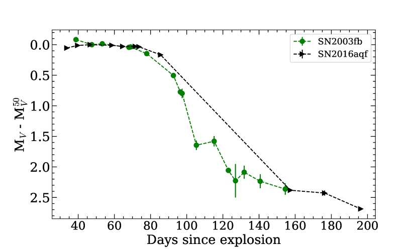
Figure 13: $V$-band comparison between the light curves of SN 2016aqf and SN 2013fb. The $y$-axis is $V$-band absolute magnitude minus $V$-band absolute magnitude at +50 days. The evolution of both light curves is very similar.

References

- Ambikasaran et al. (2015) Ambikasaran S., Foreman-Mackey D., Greengard L., Hogg D. W., O’Neil M., 2015, IEEE Transactions on Pattern Analysis and Machine Intelligence, 38, 252
- Anderson et al. (2014) Anderson J. P., et al., 2014, ApJ, 786, 67
- Anderson et al. (2016) Anderson J. P., et al., 2016, Astronomy and Astrophysics, 589, A110
- Arnett (1996) Arnett D., 1996, Supernovae and Nucleosynthesis: An Investigation of the History of Matter from the Big Bang to the Present
- Asplund et al. (2009) Asplund M., Grevesse N., Sauval A. J., Scott P., 2009, ARA&A, 47, 481
- Barbarino et al. (2015) Barbarino C., et al., 2015, MNRAS, 448, 2312
- Bersten et al. (2011) Bersten M. C., Benvenuto O., Hamuy M., 2011, ApJ, 729, 61
- Blondin et al. (2006) Blondin S., et al., 2006, AJ, 131, 1648
- Bose et al. (2013) Bose S., et al., 2013, MNRAS, 433, 1871
- Brown et al. (2013) Brown T. M., et al., 2013, PASP, 125, 1031
- Brown et al. (2016) Brown J. S., et al., 2016, The Astronomer’s Telegram, 8736, 1
- Burgh et al. (2003) Burgh E. B., Nordsieck K. H., Kobulnicky H. A., Williams T. B., O’Donoghue D., Smith M. P., Percival J. W., 2003, Prime Focus Imaging Spectrograph for the Southern African Large Telescope: optical design. pp 1463–1471, doi:10.1117/12.460312
- Buzzoni et al. (1984) Buzzoni B., et al., 1984, The Messenger, 38, 9
- Cardelli et al. (1989) Cardelli J. A., Clayton G. C., Mathis J. S., 1989, ApJ, 345, 245
- Chugai & Utrobin (2000) Chugai N. N., Utrobin V. P., 2000, A&A, 354, 557
- Collins et al. (2018) Collins C., Müller B., Heger A., 2018, MNRAS, 473, 1695
- Dessart et al. (2013a) Dessart L., Waldman R., Livne E., Hillier D. J., Blondin S., 2013a, MNRAS, 428, 3227
- Dessart et al. (2013b) Dessart L., Hillier D. J., Waldman R., Livne E., 2013b, MNRAS, 433, 1745
- Dessart et al. (2014) Dessart L., et al., 2014, MNRAS, 440, 1856
- Elmhamdi et al. (2003) Elmhamdi A., et al., 2003, MNRAS, 338, 939
- Firth et al. (2015) Firth R. E., et al., 2015, MNRAS, 446, 3895
- Fraser et al. (2012) Fraser M., et al., 2012, ApJ, 759, L13
- Gal-Yam (2017) Gal-Yam A., 2017, Observational and Physical Classification of Supernovae. Springer International Publishing, Cham, pp 195–237, doi:10.1007/978-3-319-21846-5_35, https://doi.org/10.1007/978-3-319-21846-5_35
- Gal-Yam et al. (2011) Gal-Yam A., et al., 2011, ApJ, 736, 159
- Galbany et al. (2016) Galbany L., et al., 2016, AJ, 151, 33
- Goldberg et al. (2019) Goldberg J. A., Bildsten L., Paxton B., 2019, ApJ, 879, 3
- Guillochon et al. (2017) Guillochon J., Parrent J., Kelley L. Z., Margutti R., 2017, ApJ, 835, 64
- Gutiérrez et al. (2017) Gutiérrez C. P., et al., 2017, The Astrophysical Journal, 850, 89
- Gutiérrez et al. (2018) Gutiérrez C. P., et al., 2018, Monthly Notices of the Royal Astronomical Society, 479, 3232
- Hamuy (2001) Hamuy M. A., 2001, PhD thesis, The University of Arizona
- Hamuy (2003) Hamuy M., 2003, ApJ, 582, 905
- Hamuy & Pinto (2002) Hamuy M., Pinto P. A., 2002, ApJ, 566, L63
- Harutyunyan et al. (2008) Harutyunyan A. H., et al., 2008, A&A, 488, 383
- Hosseinzadeh et al. (2016) Hosseinzadeh G., Yang Y., McCully C., Arcavi I., Howell D. A., Valenti S., 2016, The Astronomer’s Telegram, 8748, 1
- Hosseinzadeh et al. (2018) Hosseinzadeh G., et al., 2018, ApJ, 861, 63
- Jerkstrand et al. (2012) Jerkstrand A., Fransson C., Maguire K., Smartt S., Ergon M., Spyromilio J., 2012, A&A, 546, A28
- Jerkstrand et al. (2014) Jerkstrand A., Smartt S. J., Fraser M., Fransson C., Sollerman J., Taddia F., Kotak R., 2014, MNRAS, 439, 3694
- Jerkstrand et al. (2015a) Jerkstrand A., et al., 2015a, MNRAS, 448, 2482
- Jerkstrand et al. (2015b) Jerkstrand A., et al., 2015b, ApJ, 807, 110
- Jerkstrand et al. (2018) Jerkstrand A., Ertl T., Janka H. T., Müller E., Sukhbold T., Woosley S. E., 2018, MNRAS, 475, 277
- Jha & Miszalski (2016) Jha S. W., Miszalski B., 2016, The Astronomer’s Telegram, 8749, 1
- Kasen & Woosley (2009) Kasen D., Woosley S. E., 2009, ApJ, 703, 2205
- Kennicutt & Evans (2012) Kennicutt R. C., Evans N. J., 2012, Annual Review of Astronomy and Astrophysics, 50, 531
- Kobulnicky et al. (2003) Kobulnicky H. A., Nordsieck K. H., Burgh E. B., Smith M. P., Percival J. W., Williams T. B., O’Donoghue D., 2003, Prime focus imaging spectrograph for the Southern African large telescope: operational modes. pp 1634–1644, doi:10.1117/12.460315
- Kozyreva et al. (2019) Kozyreva A., Nakar E., Waldman R., 2019, MNRAS, 483, 1211
- Kozyreva et al. (2020) Kozyreva A., Nakar E., Waldman R., Blinnikov S., Baklanov P., 2020, arXiv e-prints, p. arXiv:2003.14097
- Kulkarni & Kasliwal (2009) Kulkarni S., Kasliwal M. M., 2009, in Kawai N., Mihara T., Kohama M., Suzuki M., eds, Astrophysics with All-Sky X-Ray Observations. p. 312 (arXiv:0903.0218)
- Kushnir (2015) Kushnir D., 2015, arXiv e-prints, p. arXiv:1506.02655
- Lauberts & Valentijn (1989) Lauberts A., Valentijn E. A., 1989, The surface photometry catalogue of the ESO-Uppsala galaxies
- Li et al. (2011) Li W., et al., 2011, Nature, 480, 348
- Limongi & Chieffi (2003) Limongi M., Chieffi A., 2003, ApJ, 592, 404
- Lisakov et al. (2017) Lisakov S. M., Dessart L., Hillier D. J., Waldman R., Livne E., 2017, MNRAS, 466, 34
- Lisakov et al. (2018) Lisakov S. M., Dessart L., Hillier D. J., Waldman R., Livne E., 2018, MNRAS, 473, 3863
- Litvinova & Nadezhin (1985) Litvinova I. Y., Nadezhin D. K., 1985, Soviet Astronomy Letters, 11, 145
- Lodders (2003) Lodders K., 2003, ApJ, 591, 1220
- Lyman et al. (2014) Lyman J. D., Bersier D., James P. A., 2014, Monthly Notices of the Royal Astronomical Society, 437, 3848
- Maeda et al. (2007) Maeda K., et al., 2007, The Astrophysical Journal, 658, L5
- Maeda et al. (2010) Maeda K., Taubenberger S., Sollerman J., Mazzali P. A., Leloudas G., Nomoto K., Motohara K., 2010, ApJ, 708, 1703
- Maguire et al. (2010) Maguire K., et al., 2010, MNRAS, 404, 981
- Maguire et al. (2012) Maguire K., et al., 2012, MNRAS, 420, 3451
- Makarov et al. (2014) Makarov D., Prugniel P., Terekhova N., Courtois H., Vauglin I., 2014, A&A, 570, A13
- Marino et al. (2013) Marino R. A., et al., 2013, Astronomy and Astrophysics, 559, A114
- Martinez & Bersten (2019) Martinez L., Bersten M. C., 2019, A&A, 629, A124
- Maund et al. (2013) Maund J. R., et al., 2013, MNRAS, 431, L102
- Mazzali et al. (2007) Mazzali P. A., Röpke F. K., Benetti S., Hillebrandt W., 2007, Science, 315, 825
- Müller et al. (2016) Müller B., Viallet M., Heger A., Janka H.-T., 2016, ApJ, 833, 124
- Müller et al. (2017) Müller T., Prieto J. L., Pejcha O., Clocchiatti A., 2017, ApJ, 841, 127
- Munari & Zwitter (1997) Munari U., Zwitter T., 1997, Astronomy and Astrophysics, 318, 269
- Nakaoka et al. (2018) Nakaoka T., et al., 2018, ApJ, 859, 78
- Papenkova et al. (2003) Papenkova M., Li W., Lotoss/Kait Schmidt B., Salvo M., Ford A., 2003, IAU Circ., 8143, 2
- Park & Li (2004) Park S., Li W., 2004, IAU Circ., 8431, 2
- Pastorello (2012) Pastorello A., 2012, Memorie della Societa Astronomica Italiana Supplementi, 19, 24
- Pastorello et al. (2004) Pastorello A., et al., 2004, MNRAS, 347, 74
- Pastorello et al. (2006) Pastorello A., et al., 2006, MNRAS, 370, 1752
- Pastorello et al. (2009) Pastorello A., et al., 2009, MNRAS, 394, 2266
- Pejcha & Prieto (2015) Pejcha O., Prieto J. L., 2015, ApJ, 806, 225
- Planck Collaboration et al. (2016) Planck Collaboration et al., 2016, A&A, 594, A13
- Popov (1993) Popov D. V., 1993, ApJ, 414, 712
- Poznanski et al. (2012) Poznanski D., Prochaska J. X., Bloom J. S., 2012, MNRAS, 426, 1465
- Rasmussen & Williams (2006) Rasmussen C. E., Williams C. K. I., 2006, Gaussian Processes for Machine Learning
- Richmond et al. (1994) Richmond M. W., Treffers R. R., Filippenko A. V., Paik Y., Leibundgut B., Schulman E., Cox C. V., 1994, AJ, 107, 1022
- Riess et al. (2018) Riess A. G., et al., 2018, ApJ, 855, 136
- Roy et al. (2011) Roy R., et al., 2011, ApJ, 736, 76
- Sahu et al. (2006) Sahu D. K., Anupama G. C., Srividya S., Muneer S., 2006, MNRAS, 372, 1315
- Schlafly & Finkbeiner (2011) Schlafly E. F., Finkbeiner D. P., 2011, ApJ, 737, 103
- Shappee et al. (2014) Shappee B. J., et al., 2014, ApJ, 788, 48
- Shivvers et al. (2017) Shivvers I., et al., 2017, PASP, 129, 054201
- Shussman et al. (2016) Shussman T., Nakar E., Waldman R., Katz B., 2016, arXiv e-prints, p. arXiv:1602.02774
- Smartt (2015) Smartt S. J., 2015, Publ. Astron. Soc. Australia, 32, e016
- Smartt et al. (2009) Smartt S. J., Eldridge J. J., Crockett R. M., Maund J. R., 2009, MNRAS, 395, 1409
- Smartt et al. (2015) Smartt S. J., et al., 2015, A&A, 579, A40
- Spiro et al. (2014) Spiro S., et al., 2014, MNRAS, 439, 2873
- Sukhbold et al. (2016) Sukhbold T., Ertl T., Woosley S. E., Brown J. M., Janka H. T., 2016, ApJ, 821, 38
- Takáts et al. (2014) Takáts K., et al., 2014, MNRAS, 438, 368
- Terry et al. (2002) Terry J. N., Paturel G., Ekholm T., 2002, A&A, 393, 57
- Theureau et al. (1998) Theureau G., Rauzy S., Bottinelli L., Gouguenheim L., 1998, A&A, 340, 21
- Thielemann et al. (1996) Thielemann F.-K., Nomoto K., Hashimoto M.-A., 1996, ApJ, 460, 408
- Tomasella et al. (2013) Tomasella L., et al., 2013, MNRAS, 434, 1636
- Tomasella et al. (2018) Tomasella L., et al., 2018, MNRAS, 475, 1937
- Turatto et al. (1998) Turatto M., et al., 1998, ApJ, 498, L129
- Turatto et al. (2003) Turatto M., Benetti S., Cappellaro E., 2003, in Hillebrandt W., Leibundgut B., eds, From Twilight to Highlight: The Physics of Supernovae. p. 200 (arXiv:astro-ph/0211219), doi:10.1007/10828549_26
- Utrobin & Chugai (2009) Utrobin V. P., Chugai N. N., 2009, A&A, 506, 829
- Utrobin et al. (2007) Utrobin V. P., Chugai N. N., Pastorello A., 2007, A&A, 475, 973
- Valenti et al. (2014) Valenti S., et al., 2014, MNRAS, 438, L101
- Valenti et al. (2016) Valenti S., et al., 2016, MNRAS, 459, 3939
- Van Dyk et al. (2012) Van Dyk S. D., et al., 2012, AJ, 143, 19
- Woosley & Weaver (1995) Woosley S. E., Weaver T. A., 1995, The Astrophysical Journal Supplement Series, 101, 181
- Woosley et al. (1989) Woosley S. E., Pinto P. A., Hartmann D., 1989, ApJ, 346, 395
- Yadav et al. (2020) Yadav N., Müller B., Janka H. T., Melson T., Heger A., 2020, ApJ, 890, 94
- Yaron & Gal-Yam (2012) Yaron O., Gal-Yam A., 2012, PASP, 124, 668
- Zampieri et al. (2003) Zampieri L., Pastorello A., Turatto M., Cappellaro E., Benetti S., Altavilla G., Mazzali P., Hamuy M., 2003, MNRAS, 338, 711
- Zhang et al. (2014) Zhang J., et al., 2014, ApJ, 797, 5
- de Jaeger et al. (2018) de Jaeger T., et al., 2018, Monthly Notices of the Royal Astronomical Society, 476, 4592
- de Mello et al. (1997) de Mello D., Benetti S., Massone G., 1997, International Astronomical Union Circular, 6537, 1