NECI: N-Electron Configuration Interaction with an emphasis on state-of-the-art stochastic methods

Abstract

We present NECI, a state-of-the-art implementation of the Full Configuration Interaction Quantum Monte Carlo algorithm, a method based on a stochastic application of the Hamiltonian matrix on a sparse sampling of the wave function. The program utilizes a very powerful parallelization and scales efficiently to more than 24000 CPU cores. In this paper, we describe the core functionalities of NECI and recent developments. This includes the capabilities to calculate ground and excited state energies, properties via the one- and two-body reduced density matrices, as well as spectral and Green’s functions for ab initio and model systems. A number of enhancements of the bare FCIQMC algorithm are available within NECI, allowing to use a partially deterministic formulation of the algorithm, working in a spin-adapted basis or supporting transcorrelated Hamiltonians. NECI supports the FCIDUMP file format for integrals, supplying a convenient interface to numerous quantum chemistry programs and it is licensed under GPL-3.0.
This article has been accepted by the Jouranl of Chemical Physics, after it is published, it will be found at https://aip.scitation.org/journal/jcp.

I Introduction

O= O↑ m #3 $#2$ #1  
NECI started off in the late 1990s as an exact diagonalisation code for model quantum dots Alavi (2000); Thompson and Alavi (2002), and has evolved into a code to perform stochastic diagonalisation of large fermionic systems in finite but large quantum chemical basis sets, using the Full Configuration Interaction Quantum Monte Carlo (FCIQMC) algorithm Booth, Thom, and Alavi (2009). This algorithm samples Slater determinant (i.e. antisymmetrized) Hilbert spaces using signed walkers, by propagation of the walkers through stochastic application of the second-quantized Hamiltonian onto the walker population. In philosophy, it is similar to the continuum real-space Diffusion Monte Carlo (DMC) algorithm. However, unlike DMC, no fixed node approximation needs to be applied. Instead, the nodal structure of the wavefunction, as encoded by the signed coefficients of the sampled Slater determinants, emerges from the dynamics of the simulation itself. However, being based on an FCI parametrization of the wave function, the FCIQMC method exhibits a steep scaling with the number of electrons and is thus only suited for relatively small chemical systems compared to those accessible to DMC. While the common energy measures in FCIQMC methods, namely the projected, trial energies (cf section IV) and the energy "shift", are not variational, a variational energy can be computed from two parallel FCIQMC calculations either directly (cf section VI), or via the reduced density matrix (RDM) based energy estimator (cf section VII).

There are also similarities between the FCIQMC approach and the Auxiliary-Field Quantum Monte Carlo (AFQMC) methodBlankenbecler, Scalapino, and Sugar (1981); Sugiyama and Koonin (1986); Zhang and Krakauer (2003), both being stochastic projector techniques formulated in second quantized spaces. The latter however works in an over-complete space of non-orthogonal Slater determinants and relies on the phase-less approximation Zhang, Carlson, and Gubernatis (1997) to eliminate the phase problem associated with the Hubbard-Stratonovich transformation of the Coulomb interaction kernel, the quality of this approximation being reliant on the trial wavefunction used to constrain the path. The objective of AFQMC is the measurement of observables such as the energy by sampling over the Hubbard-Stratonovich fields. FCIQMC on the other hand works in a fixed Slater determinant space and relies on walker annihilation to overcome the fermion sign problem. The phase-less approximation renders the AFQMC method polynomial scaling, with an uncontrolled approximation, while i-FCIQMC, which is an in principle exact method, remains exponential scaling. Finally FCIQMC provides a direct measure of the CI amplitudes of the many-body wavefunction expressed in the given orbital basis, from which observables can be computed including elements of reduced density matrices (which do not commute with the Hamiltonian) via pure estimators. Exact symmetry constraints, including total spin, can be incorporated into the formalismDobrautz, Smart, and Alavi (2019). In this sense, the FCIQMC method is closer in spirit to multi-reference CI methods used in quantum chemistry to study multi-reference problems rather than the AFQMC method.

In its original formulation, the algorithm is guaranteed to converge onto the ground-state wavefunction in the long imaginary-time propagation limit, provided a sufficient number of walkers is used. This number is generally found to scale with the Hilbert space size, and is a manifestation of the sign-problem in this method, essentially implying an exponential memory cost in order to guarantee stable convergence onto the exact solution. In the subsequent development of the initiator method (i-FCIQMC)Cleland, Booth, and Alavi (2010), this condition was relaxed to allow for stable simulations at relatively low walker populations, much smaller than the full Hilbert space size, albeit at the cost of a systematically improvable bias. While the initiator adaptation removes the strict need for a minimum walker number, it does not eliminate the exponential scaling of the method, such that calculations become more and more challenging with increasing system size. To give an idea of the capabilities of the NECI implementation, estimates for the accessible system sizes are given below. The rate of convergence of the initiator error with walker number has been found to be slow for large systems. This is a manifestation of size-inconsistency error which generally plagues linear Configuration Interaction methods. A very recent development of the adaptive shift method Ghanem, Lozovoi, and Alavi (2019), mitigates this error substantially, enabling near-FCI quality results to be obtained for systems as large as benzene.

The development of the semi-stochastic method by Umrigar et al. Petruzielo et al. (2012) and its further refinements Blunt et al. (2015a) dramatically reduced the stochastic noise and hence improved the efficiency of the method.

The FCIQMC algorithm, as well as its semi-stochastic and initiator versions, are scalable on large parallel machines, thanks to the fact that walker distribution can be distributed over many processors with relatively small communication overhead. The methods, however, are not embarrassingly parallel, owing to the annihilation step of the algorithm (see also figure  1). For this reason, parallelisation over very large numbers of processors is a highly non-trivial task, but substantial progress has been made, and here we show that efficient parallelisation up to more than 24000 CPU cores can be achieved with the current NECI code.

The FCIQMC method has been generalised to excited states Blunt et al. (2015b) of the same symmetry as the ground state and to the calculation of pure one-and two-particle reduced density matrices via the "replica-trick" Zhang and Kalos (1993); Overy et al. (2014); Blunt et al. (2014); Blunt, Booth, and Alavi (2017) (and more recently three and four-particle RDMs Anderson, Shiozaki, and Booth (2020)). The availability of RDMs enabled the development of the Stochastic CASSCF method Li Manni, Smart, and Alavi (2016); Thomas et al. (2015a) for treating extremely large active spaces. More recently, a fully spin-adapted formulation of FCIQMC has been implemented based on the Graphical Unitary Group Approach Dobrautz, Smart, and Alavi (2019), which overcomes the previous limitations of spin-adaptation, which severely limited the number of open-shell orbitals which could be handled. Other advanced developments of FCIQMC in the NECI code include real-time propagation and application to spectroscopy Guther et al. (2018), Krylov-space FCIQMC Blunt et al. (2015a), and the similarity transformed FCIQMC Luo and Alavi (2018); Dobrautz, Luo, and Alavi (2019); Cohen et al. (2019); Jeszenszki, Alavi, and Brand (2019) which allows the direct incorporation of Jastrow and similar factors depending on explicit electron-electron variables into the wavefunction.

A number of stochastic methods have been developed as an extension or variation of the FCIQMC approach. These include density matrix quantum Monte Carlo (DMQMC), which allows the exact thermal density matrix to be sampled at any given temperature, and also allows straightforward estimation of general observables, including those which do not commute with the HamiltonianBlunt et al. (2014); Malone et al. (2015). Applications of DMQMC include providing accurate data for the warm dense electron gasMalone et al. (2016). Although not implemented in NECI, DMQMC is available in the HANDE-QMC codeSpencer et al. (2019).

The FCIQMC method has lead to the development of a number of highly efficient deterministic selected CI methods, including the adaptive sampling CI method of Head-Gordon and co-workers Tubman et al. (2016), who also establish the connection with the much older perturbatively selected CIPSI method of Malrieu et al Huron, Malrieu, and Rancurel (1973) but with a modified search procedure, while the Heat-Bath CI method of Umrigar and coworkers Holmes, Tubman, and Umrigar (2016) was developed from the Heat-Bath excitation generation for FCIQMC Holmes, Changlani, and Umrigar (2016) together with an initiator-like criterion to select the connected determinants with extreme efficiency. Later a sign-problem-free semi-stochastic evaluation of the Epstein-Nesbet perturbation energy was developed by Sharma et al Sharma et al. (2017) to compute the missing dynamical correlation energy at second-order in a memory and CPU efficient manner. Other highly related developments to FCIQMC which originate in the numerical analysis literature include the Fast Randomised Iteration Lim and Weare (2017) and further developments by Weare, Berkelbach and coworkers Greene et al. (2019), and co-ordinate descent FCI of Lu and coworkers Wang, Li, and Lu (2019).

Depending on the utilized features, the number of electrons and accessible basis sizes can vary. The i-FCIQMC implementation including the semi-stochastic version is highly scalable and has been successfully applied to Hilbert space sizes of up to $10^{108}$ with 54 electrons Shepherd et al. (2012). Atomic basis sets up to aug-cc-pCV8Z for first-row atoms (1138 spin orbitals) are treatable Dattani et al. (2020). Reduced density matrices can routinely be calculated for use in accurate Stochastic-MCSCF Li Manni, Smart, and Alavi (2016, 2016) for active spaces containing up to 40 electrons and 38 spatial orbitalsLi Manni and Alavi (2018); Li Manni et al. (2019). Real-time calculations are computationally more demanding but can still be performed for first-row dimers using cc-pVQZ basis sets Guther et al. (2018). For the similarity transformed FCIQMC method, the limiting factor is not the convergence of the FCIQMC, but the storage of the three-body interaction terms imposing a limit of $\sim 100$ spatial orbitals on currently available hardware Cohen et al. (2019). Optimized implementations for the application to lattice model systems, like the HubbardHubbard (1963) (in a real- and momentum space formulation), $t-J$ and the Heisenberg models for a variety of lattice geometries, are implemented in NECI . The applicability of FCIQMC to the Hubbard model strongly depends on the interaction strength $U/t$. For the very weakly correlated regime $U/t<1$, FCIQMC is employable up to 70 lattice sites Shepherd, Scuseria, and Spencer (2014), using a momentum-space basis. In the interesting, yet most problematic, intermediate interaction strength regime in two dimensions, the transcorrelated (similarity-transformed) FCIQMC is necessary to obtain reliable energies in systems up to 50 sites (at and near half-filling)Dobrautz, Luo, and Alavi (2019).

The FCIQMC algorithm as implemented in NECI is based on a sparse representation of the wave function and a stochastic application of the Hamiltonian. We start with the full wave function

$$\ket{\psi_{\text{FCI}}}=\sum_{i}C_{i}\ket{D_{i}}\,,$$ (1)

with coefficients $C_{i}$ in a many-body basis $\ket{D_{i}}$. NECI supports Slater determinants or CSFs as a many-body basis, for simplicity, for now, the usage of determinants is assumed, but the algorithm is analogous for CSFs, see also section  XII.2.2. The FCIQMC wave function is not normalized. The ground state of a Hamiltonian $\hat{H}$ is now obtained by iterative imaginary time-evolution, with the propagator expanded to first order using a discrete time-step $\Delta\tau$ such that

$$\ket{\psi(\tau+\Delta\tau)}=\left(1-\Delta\tau(\hat{H}-S(\tau))\right)\ket{\psi(\tau)}\,,$$ (2)

which converges to the ground state of $\hat{H}$ for $\tau\rightarrow\infty$ for $|\Delta\tau|<\frac{2}{W}$ where $W$ is the difference between the largest and smallest eigenvalue of $\hat{H}$Trivedi and Ceperley (1990). Here, $S(\tau)$ is a diagonal shift applied to $\hat{H}$, which is iteratively updated to match the ground state energy.

The full wave function is stored in a compressed manner, where only coefficients above a given threshold value $C_{\text{min}}$ are stored. Coefficients smaller than $C_{\text{min}}$ are stochastically rounded. That is, in every iteration, a wave function given by coefficients $C_{i}(\tau)$ is stored such that

$$C_{i}(\tau)=\begin{cases}C_{i}&\mathrm{if}\;|C_{i}|>C_{\text{min}}\\ \mathrm{sign}(C_{i})\,C_{\text{min}}&\mathrm{else\;w.\;prob\;}\frac{|C_{i}|}{C_{\text{min}}}\\ 0&\mathrm{otherwise}\end{cases}\,,$$ (3)

such that $\Braket{C_{i}(\tau)}=C_{i}$. This compression is applied in every step of the algorithm that affects the coefficients. The value $|C_{i}(\tau)|$ is referred to as walker number of the determinant $\ket{D_{i}}$, so $\ket{D_{i}}$ is said to have $|C_{i}(\tau)|$ walkers assigned.

Applying the Hamiltonian to this compressed wave function is done by separating it into a diagonal and an off-diagonal part as

$$\ket{\psi(\tau+\Delta\tau)}= \underbrace{\sum_{i}\left(1-\Delta\tau(H_{ii}-S(\tau))\right)C_{i}(\tau)\ket{D_{i}}}_{\text{(b) Death step}}\overarrow[-][\downarrow]{(c)Annihilationstep}$$

$$\underbrace{\sum_{i}\sum_{j\neq i}\Delta\tau H_{ji}C_{i}(\tau)\ket{D_{j}}}_{\text{(a) Spawn step}}\,,$$ (4)

and then performed in the three labeled steps $(a)-(c)$. First, in the spawning step, the off-diagonal part is evaluated by stochastically sampling the sum over $j$, storing the resulting spawned wave-function as a separate entity as described in the flow chart in Figure 1. Then, in the death step, the diagonal contribution is evaluated deterministically, following a stochastic rounding of the resulting coefficients. This step is performed in-place, since the coefficients of the previous iterations are not required anymore. Finally, the spawned wave-function from the off-diagonal part is added in the annihilation step, summing up all contributions from the spawned wave-function to each determinant. NECI implements the initiator method, too, which labels a class of determinants as initiators, typically those with an associated walker number above a given threshold, and effectively zeroes all matrix elements between non-initiator determinants and determinants with $C_{i}(\tau)=0$. The implementation thereof is also sketched in figure 1.

In the context of FCIQMC calculations, the core functionality of NECI consists of a highly parallelizable implementation of the initiator FCIQMC method Cleland, Booth, and Alavi (2010) for both real and complex Hamiltonians. There is both a generic interface for ab initio systems, specialized implementations for the Hubbard and Heisenberg models, as well as the uniform electron gas. The interface for passing input information on the system to NECI is discussed in section XIV. To enable continuation of calculations at a later point, NECI can write the instantaneous wave function and current parameters—such as the shift value—to disk, saving the current state of the calculation.

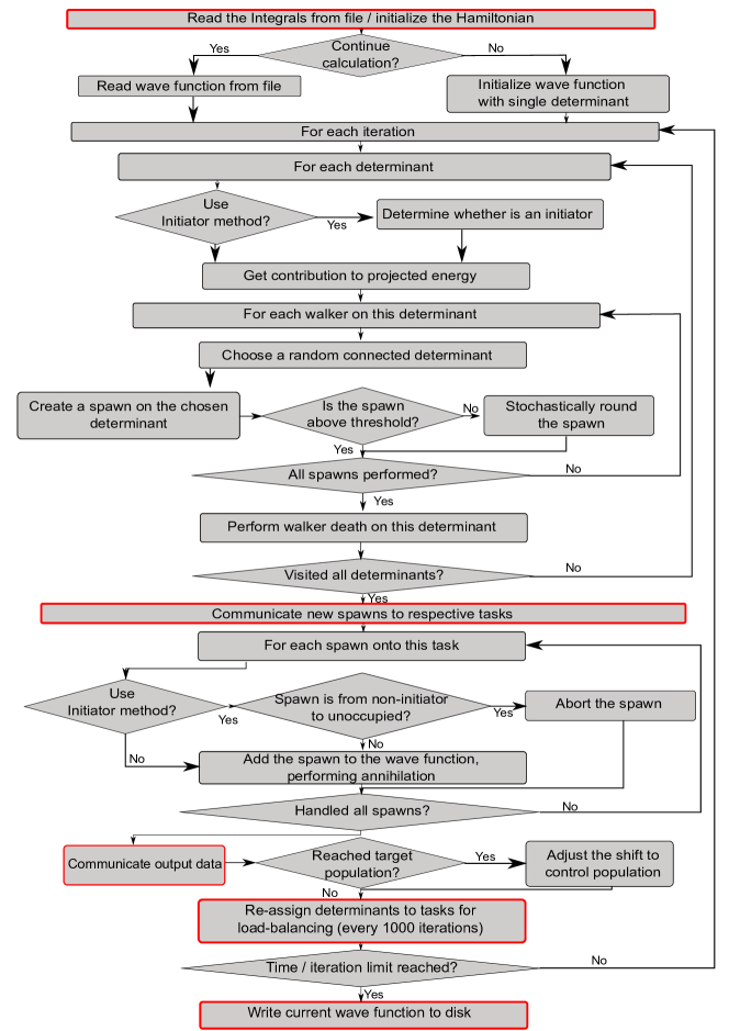
Figure 1: Flow chart showing the basic initiator-FCIQMC implementation in NECI . Marked in red are steps that require synchronisation between the MPI tasks and thus are not trivially parallelizable.

The NECI program Booth and Alavi et. al. (2013) itself is written in Fortran, and requires extended Fortran 2003 support, which is the default for current Fortran compilers. Parallelization is achieved using the Message Passing Interface (MPI) Clarke, Glendinning, and Hempel (1994), and support for MPI 3.0 or newer is required. NECI further requires the BLAS Blackford et al. (2002) and LAPACK Anderson et al. (1999) lineara algebra libraries, which are available in numerous packages. Usage of the HDF5 library The HDF Group (NNNN) for parallel I/O is supported, but not required. If used, the linked HDF5 library has to be built with Fortran support and for parallel applications. For installation, cmake is required, as well as the fypp Fortran preprocessorAradi . For pseudo random number generation, the double precision SIMD oriented fast Mersenne Twister (dSFMT) Saito and Matsumoto (2008a, b) implementation of the Mersenne Twister method Matsumoto and Nishimura (1998) is used. The stable version of the program can be obtained from github at https://github.com/ghb24/NECI_STABLE, licensed under the GNU General Public License 3.0. Some advanced or experimental features are only contained in the development version, for access to the development version, please contact the corresponding authors. All features presented here are eventually to be integrated to the stable version. Detailed instructions on the installation can be found in the Documentation that is available together with the code.

In the following, various important features of NECI are explained in detail. An overview of excitation generation, a fundamental part of every FCIQMC calculation, is given in section II. Then, the semi-stochastic approach (section III), the estimation of energy and use of trial wave functions (section IV), the recently proposed adaptive shift method to reduce the initiator error (section V) and perturbative corrections to this error (section VI), the sampling of reduced density matrices which is crucial for interfacing the FCIQMC method with other algorithms (section VII), the calculation of excited states (section VIII), static response functions (section IX and the real-time FCIQMC method (section X), the transcorrelated approach (section XI) and the available symmetries, including total spin conservation utilizing GUGA (section  XII) are discussed. Finally, the scalability of NECI is explored (section XIII) and the interfaces for usage with other code are presented (section XIV), in particular for the Stochastic-MCSCF method (section XV).

II Excitation generation

A key component of the FCIQMC algorithm is the sampling of the Hamiltonian matrix elements in the spawning step, where the Hamiltonian is applied stochastically. This requires an efficient algorithm to randomly generate connected determinants with a known probability $p_{gen}$ for any given determinant, referred to as excitation generation. This typically means making a symmetry constrained choice of (up to) two occupied orbitals in a determinant and (up to) two orbitals to replace them with, such that the corresponding Hamiltonian matrix element is non-zero. If spin-adapted functions are used rather than determinants, the connectivity rules change but the main principles are same.

The spawning probability for a spawn from a determinant $\ket{D_{i}}$ to a determinant $\ket{D_{j}}$ is in practice given by

$$p_{s}=\Delta\tau\frac{|H_{ij}|}{p_{gen}(j|i)}\,.$$ (5)

This means, the purpose of $p_{gen}(j|i)$ of selecting $\ket{D_{j}}$ from $\ket{D_{i}}$ in the spawning probability $p_{s}$ is to allow the flexibility in the selection of determinants $\ket{D_{j}}$ from $\ket{D_{i}}$ so that, irrespective of how we choose $\ket{D_{j}}$ from $\ket{D_{i}}$, the rate at which transitions occur is not biased by the selection algorithm. In other words, if a particular determinant $\ket{D_{j}}$ is only selected rarely from $\ket{D_{i}}$ (i.e. with low generation probability), then the acceptance of the move (i.e. the spawning probability) will be with correspondingly high probability (i.e. proportional to the inverse of the generation probability). Conversely if a determinant $\ket{D_{j}}$ is selected with relatively high generation probability from $\ket{D_{i}}$, then its acceptance probability will be correspondingly low. In other words, from the point of view of the exactness of the FCIQMC algorithm, the precise manner in which excitations are made is immaterial: as long as the probability $p_{gen}(j|i)>0$ when $|H_{ij}|>0$, the algorithm will ensure that transitions from $D_{i}\rightarrow D_{j}$ occur at a rate proportional to $|H_{ij}|$, and hence the walker dynamics converges onto the exact ground-state solution of the Hamiltonian matrix. However, from the point of view of efficiency, different algorithms to generate excitations are by no means equivalent.

That is, events with a very large $\frac{|H_{ij}|}{p_{gen}(j|i)}$ can lead to very large spawns and thus endanger the stability of an i-FCIQMC calculation. For time-step optimization, NECI offers a general histogramming method, which determines the time-step from a histogram of $\frac{|H_{ij}|}{p_{gen}(j|i)}$ Dobrautz, Smart, and Alavi (2019), as well as an optimized special case thereof, which only takes into account the maximal ratio Smart (2014). If required, internal weights of the excitation generators such a bias towards double excitations are then optimized in the same fashion to maximise the time-step.

However, as a result, the time-step and thus overall efficiency of the simulation is driven by the worst-cases of the $\frac{|H_{ij}|}{p_{gen}(j|i)}$ ratio discovered within the explored Hilbert space. Thus an optimal excitation generator should create excitations with a probability distribution to the Hamiltonian matrix elements, such that

$$\frac{|H_{ij}|}{p_{gen}(j|i)}\approx\mathrm{const.}$$ (6)

This is the optimal probability distribution, since then, the acceptance rate is solely determined by the time step Holmes, Changlani, and Umrigar (2016).

NECI supports a variety of algorithms to perform excitation generation, with the most notable being the pre-computed heat-bath (PCHB) sampling (a variant of the heat-bath sampling presented in Holmes, Changlani, and Umrigar (2016), as described in the appendix  A.3), the on-the-fly Cauchy-Schwartz method Smart, Booth, and Alavi (described in the appendix  A.2), the pre-computed Power-Pitzer method Neufeld and Thom (2019) and lattice-model excitation generators both for real-space and momentum-space lattices. Additionally, a three-body excitation generator and a uniform excitation generator are available, which are essential for treating systems with the transcorrelated ansatz when including three-body interactions.

As heat-bath excitation generation can have high memory requirements, it might be impractical for some systems. There, the on-the-fly Cauchy-Schwartz method can maintain very good $\frac{|H_{ij}|}{p_{gen}(j|i)}$ ratios without significant memory cost, albeit at $\mathcal{O}(N)$ computational cost, $N$ being the number of orbitals, and possibly with dynamic load imbalance. The details of the Cauchy-Schwartz excitation generation are discussed in the appendix.

III Semi-stochastic FCIQMC

In many chemical systems the wave function is dominated by a relatively small number of determinants. In a stochastic algorithm, the efficiency can be improved substantially by treating these determinants in a partially deterministic manner.

Petruzielo et al. suggested a semi-stochastic algorithmPetruzielo et al. (2012), where the FCIQMC projection operator $\hat{P}=\sum_{ij}P_{ij}|D_{i}\rangle\langle D_{j}|$, is applied exactly within a small but important subspace, which we call the deterministic space, $\mathcal{D}$. Specifically, we write

$$\hat{P}=\hat{P}^{\mathcal{D}}+\hat{P}^{\mathcal{S}},$$ (7)

where

$$\hat{P}^{\mathcal{D}}=\sum_{i\in\mathcal{D},\,j\in\mathcal{D}}P_{ij}|D_{i}\rangle\langle D_{j}|.$$ (8)

The $\hat{P}^{\mathcal{D}}$ operator therefore accounts for all spawnings which are both from and to determinants in $\mathcal{D}$. The stochastic projection operator, $\hat{P}^{\mathcal{S}}$, contains all remaining terms. The matrix elements of $\hat{P}^{\mathcal{D}}$ are calculated and stored in a fixed array, and applied exactly each iteration by a matrix-vector multiplication. The operator $\hat{P}^{\mathcal{S}}$ is then applied stochastically by the usual FCIQMC spawning algorithm.

The semi-stochastic adaptation requires storing the Hamiltonian matrix within $\mathcal{D}$, which we denote $\bm{H}^{\mathcal{D}}$. In NECI, $\bm{H}^{\mathcal{D}}$ is stored in a sparse format, distributed across all processes. To calculate $\bm{H}^{\mathcal{D}}$, we have implemented the fast generation scheme of Li et al.Li et al. (2018) This approach has allowed us to use deterministic spaces containing up to $\sim 10^{7}$ determinants. However, a more typical size of $\mathcal{D}$ is between $10^{4}$ and $10^{5}$.

Ideally, a deterministic space of a given size ($N_{\mathcal{D}}$) should be chosen to contain the determinants with the largest value of $|C_{i}|$ in the exact FCI wave function. This optimal choice is not possible in practice, but various approaches exist to make an approximate selection. Umrigar and co-workers suggest using selected configuration interaction (SCI) to make the selection.Petruzielo et al. (2012) Within NECI, the most common approach is to choose the $N_{\mathcal{D}}$ determinants which have the largest weight in the FCIQMC wave function, at a given iteration.Blunt et al. (2015a) Therefore, a typical FCIQMC simulation in NECI will be performed until convergence (at some iteration number $N_{\mathrm{conv.}}$) using the fully-stochastic algorithm, at which point the semi-stochastic approach is turned on, selecting the $N_{\mathcal{D}}$ most populated determinants in the instantaneous wave function to form $\mathcal{D}$. The appropriate parameters ($N_{\mathcal{D}}$ and $N_{\mathrm{conv.}}$) are specified in the NECI input file. NECI supports performing periodic re-evaluation of the $N_{\mathcal{D}}$ most populated determinants, updating the deterministic space $\mathcal{D}$ with a given frequency.

Using the semi-stochastic adaptation with a moderate deterministic space (on the order of $\sim 10^{4}$) can improve the efficiency of FCIQMC by multiple orders of magnitudes. This is particularly true in weakly correlated systems. The semi-stochastic approach can also be used in NECI when sampling reduced density matrices (RDMs) as described in section VII. Here, contributions to RDMs are included exactly between all pairs of determinants within $\mathcal{D}$. It has been shown that this can substantially reduce the error on RDM-based estimators.Blunt et al. (2015a) Using the semi-stochastic adaptation in NECI disables the load-balancing unless a periodic update of $\mathcal{D}$ is performed.

IV Trial wave functions

The most common energy estimator used in FCIQMC is the reference-based projected estimator,

$$E_{\mathrm{Ref}}=\frac{\langle D_{\mathrm{Ref}}|\hat{H}|\Psi\rangle}{\langle D_{\mathrm{Ref}}|\Psi\rangle},$$ (9)

where $|D_{\mathrm{Ref}}\rangle$ is an appropriate reference determinant (usually the Hartree–Fock determinant). In case $\ket{\Psi}$ is an eigenstate, this yields the exact energy, but in general it is a non-variational estimator. This is the default estimator for the energy, and can be obtained with minimal overhead.

NECI has the option to use projected estimators based on more accurate trial wave functions, which can significantly reduce statistical error in energy estimates. For this reason we define a trial subspace $\mathcal{T}$, which is spanned by $N_{\mathcal{T}}$ determinants. Similarly to the deterministic space, $\mathcal{T}$ should ideally be formed from the determinants with the largest contribution in the FCI wave function, or some good approximation to these determinants. Projecting $\hat{H}$ into $\mathcal{T}$ gives us a $N_{\mathcal{T}}\times N_{\mathcal{T}}$ matrix, which we denote $\bm{H}^{\mathcal{T}}$, whose eigenstates can be used as trial wave functions for more accurate energy estimators.

Let us denote an eigenstate of $\bm{H}^{\mathcal{T}}$ by $|\Psi^{\mathcal{T}}\rangle=\sum_{i\in\mathcal{T}}C_{i}^{\mathcal{T}}|D_{i}\rangle$, with eigenvalue $E^{\mathcal{T}}$. Then a trial function-based estimator can be defined as

$$E_{\mathrm{Trial}} =\frac{\langle\Psi^{\mathcal{T}}|\hat{H}|\Psi\rangle}{\langle\Psi^{\mathcal{T}}|\Psi\rangle},$$ (10)

$$=E^{\mathcal{T}}+\frac{\sum_{j\in\mathcal{C}}C_{j}V_{j}}{\sum_{i\in\mathcal{T}}C_{i}C_{i}^{\mathcal{T}}}.$$ (11)

Here, $\mathcal{C}$ is the space of all determinants connected to $\mathcal{T}$ by a single application of $\hat{H}$ (not including those in $\mathcal{T}$). $C_{i}$ denotes walker coefficients in the FCIQMC wave function, and $V_{j}$ is defined within $\mathcal{C}$ as

$$V_{j}=\sum_{i\in\mathcal{T}}\bra{D_{j}}\hat{H}\ket{D_{i}}C_{i}^{\mathcal{T}},\;\;\;\;\;\;\;\;|D_{j}\rangle\in\mathcal{C},\;\ket{D_{i}}\in\mathcal{T}.$$ (12)

To calculate the estimator $E_{\mathrm{Trial}}$ we therefore require several large arrays: first, $\bm{H}^{\mathcal{T}}$, which is stored in a sparse format, in the same manner as the deterministic Hamiltonian in the semi-stochastic scheme; second, $\ket{\psi^{\mathcal{T}}}$, which must be calculated by the Lanczos or Davidson algorithm; third, $\bm{V}$, which is a vector in the entire $\mathcal{C}$ space. The number of coefficients to store in $\mathcal{C}$ is larger than in $\mathcal{T}$ by a significant amount, typically by several orders of magnitude. Indeed, storing $\mathcal{V}$ can become the largest memory requirement. Because of this, using trial wave functions is typically more memory intensive in NECI than using the semi-stochastic approach, for a given space size. We therefore suggest using a smaller trial space, $\mathcal{T}$, compared to the deterministic space, $\mathcal{D}$.

Note that the initiator error on $E_{\mathrm{Trial}}$ is not the same as the initiator error on $E_{\mathrm{Ref}}$. For example, $E_{\mathrm{Trial}}$ becomes exact as $|\Psi^{\mathcal{T}}\rangle$ approaches the FCI wave function. For practical trial wave functions, however, the two energy estimates typically give similar initiator errors for ground-state energies in our experience. An exception occurs for excited states (see Section VIII). In this case, the wave function is usually not well approximated by a single reference determinant, and $E_{\mathrm{Trial}}$ with an appropriate $\mathcal{T}$ yields a great improvement, both for the statistical and initiator error.

V Adaptive Shift

The initiator criterion Cleland, Booth, and Alavi (2010) is important in making FCIQMC a practical method allowing us to achieve convergence at a dramatically lower number of walkers than the full FCIQMC Booth, Thom, and Alavi (2009). However, this approximation introduces a bias in the energy when an insufficient number of walkers is used. This bias can be attributed to the fact that non-initiators are systematically undersampled due to the lack of feedback from their local Hilbert space. To correct this, we can allow each non-initiator determinant $\ket{D_{i}}$ to have its own local shift $S_{i}(\tau)$ as an appropriate fraction of the full shift $S(\tau)$

$$S_{i}(\tau)=f_{i}\times S(\tau)\;.$$ (13)

The fraction $f_{i}$ is computed by monitoring which spawns are accepted due to the initiator criterion and accumulating positive weights over the accepted and rejected ones:

$$f_{i}=\frac{\sum_{j\in accepted}w_{ij}}{\sum_{j\in all}w_{ij}}\;.$$ (14)

These weights $w_{ij}$ are derived from perturbation theory Lowdin (1951) where the first-order contribution of determinant $\ket{D_{i}}$ to the amplitude of determinant $\ket{D_{j}}$ is used as a weight for spawns from $\ket{D_{i}}$ to $\ket{D_{j}}$

$$w_{ij}=\frac{|H_{ij}|}{H_{jj}-E_{0}}\;.$$ (15)

It is worth noting that, regardless of how the weights are chosen, expression (14) guarantees that initiators get the full shift. Also as the number of walkers increases, the local Hilbert space of a non-initiator becomes more and more populated, restoring the full method in the large walker limit.

We call the above approach for unbiasing the initiator approximation, the adaptive-shift method Ghanem, Lozovoi, and Alavi (2019). In Fig. 2, examplary results (from  Ghanem, Lozovoi, and Alavi (2019)) from using the adaptive shift method are displayed, comparing total energies of the butadiene molecule in ANO-L-pVDZ basis (22 electrons in 82 spatial orbitals), obtained with the normal initiator method and the adaptive shift method using three different values of the initiator parameter $n_{a}$ : 3, 10 and 20. The adaptive shift results are in good agreement with other benchmark values from DMRG, CCSDT(Q) and extrapolated HCIPT2. In contrast, the normal initiator method has a bias of over 10 mH. Also notice how by using the adaptive shift, the results become, to a large extent, independent of the initiator parameter $n_{a}$.

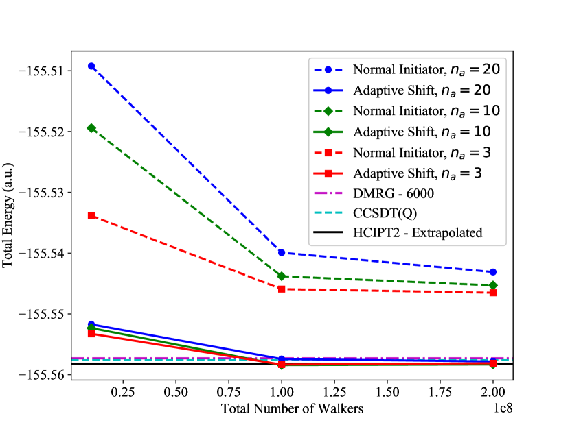
Figure 2: Example of application of the adaptive shift method: Total energies of butadiene for the normal initiator and the adaptive shift method, as a function of the number of walkers, for three values of the initiator parameter $n_{a}$. The adaptive shift results converge to: $-155.5581(2)\,\mathrm{E_{h}}$, $-155.5583(2)\,\mathrm{E_{h}}$ and $-155.5578(2)\,\mathrm{E_{h}}$ for $n_{a}$ of 3, 10 and 20, respectively. The DMRG value of $-155.5573\,\mathrm{E_{h}}$, obtained with a bond dimension of 6000 Olivares-Amaya et al. (2015), the CCSDT(Q) value of $-155.5576\,\mathrm{E_{h}}$ and the extrapolated HCIPT2 value of $-155.5582(1)\,\mathrm{E_{h}}$ Chien et al. (2018) are in good agreement with that. Reproduced from Ghanem et al. JCP 151, 224108 (2019) Ghanem, Lozovoi, and Alavi (2019) with the permission of AIP Publishing.

VI Perturbative corrections to initiator error

An alternative approach to removing initiator error in NECI is through a perturbative correctionBlunt (2018). In the initiator approximation, spawning events from non-initiators to unoccupied determinants are typically discarded. These discarded events make up a significant fraction of all spawning attempts made, which in turn accounts for much of the total simulation time. While it is necessary to discard these spawned walkers to prevent disastrous noise from the sign problemSpencer, Blunt, and Foulkes (2012), this step is extremely wasteful.

These discarded walkers actually contain significant information which can be used to greatly increase the accuracy of the initiator FCIQMC approach. Specifically, these walkers may sample up to double excitations from the currently-occupied determinants (a similar argument can be used to justify the above adaptive shift approach). In analogy with a comparable approach taken in selected CI methods, these discarded walkers can be used to sample a second-order correction to the energy from Epstein-Nesbet perturbation theory.

The correction is calculated by

$$\Delta E_{2}=\frac{1}{(\Delta\tau)^{2}}\sum_{i\,\in\,\textrm{rejected}}\frac{S_{i}^{1}S_{i}^{2}}{E_{0}-H_{ii}}.$$ (16)

Here, $\Delta\tau$ is the time step, $E_{0}$ is the i-FCIQMC estimate of the energy, and $S_{i}^{r}$ is the total spawned weight onto determinant $|D_{i}\rangle$ in replica $r$ (the replica approach will be discussed in more detail in Section VII). This correction requires that two replica FCIQMC simulations are being performed simultaneously, to avoid biases in this estimator. The summation here is performed over all spawning attempts which are discarded on both replicas simultaneously.

This must only be applied to correct the variational energy estimator from i-FCIQMC. Such variational energies in NECI can either be calculated directlyBlunt, Thom, and Scott (2019); Blunt (2019), or from two-body reduced density matrices, which may be sampled in FCIQMC.

This perturbative correction is essentially free to accumulate, since all spawned walkers contributing to Eq. (16) are created regardless. The only significant extra cost comes from the requirement to perform two replica simulations. However, for large systems the noise on this correction can become significant, which necessitates further running time to reduce statistical errors.

This correction has proven extremely successful in practice, particularly for weakly correlated systems, where it is typical to see $80-90\%$ of remaining initiator error removedBlunt (2018); Blunt, Thom, and Scott (2019); Blunt (2019).

VII Density matrix sampling and pure expectation values

While the total energy is an important quantity to extract from quantum systems, a more complete characterization of a system requires the ability to extract information about other expectation values. If these expectation values are derived from operators which do not commute with the Hamiltonian of the system, then a ‘projected’ estimate of the expectation value akin to Eq. 9 is not possible, and alternatives within FCIQMC are required in order to compute them. This is the case for many key quantities such as nuclear derivatives (forces on atoms), dipole moments and higher-order electrical moments, as well as other observables such as pair distribution functions Thomas et al. (2015b). They all can be obtained via the corresponding $n$-body reduced density matrix ($n$-RDM), where $n$ is the rank of the operator in question, that fully characterizes the correlated distribution and coherence of $n$ electrons relative to each other. This information can also be used to calculate quantum information measures, which are not observables but which characterize the entanglement within a system, such as correlation entropies Overy et al. (2014).

To characterize the strength of coupling between different states under certain operators, e.g. the oscillator strength of optical excitations, as well as obtaining other dynamical information requires computing transition density matrices (tRDMs) between stochastic samples of different states, which can be sampled within FCIQMC using the excited state feature discussed in section VIII Booth and Chan (2012); Blunt, Booth, and Alavi (2017). Furthermore, the two states considered may not sample eigenstates of the system, but one of them can be a response state of the system, then the resulting tRDMs characterize the response of a system to a perturbation, corresponding to a higher derivative of the energy such as the polarizability of the system, which will be addressed in section IX Samanta, Blunt, and Booth (2018). Finally, RDMs can also be used to characterize the expectation value of an effective Hamiltonian in a subspace of a system Blunt, Alavi, and Booth (2015, 2018). This effective Hamiltonian can include effects such as electronic correlations coupling the space to a wider external set of states. The plurality of electronic structure methods of this kind, such as explicitly correlated ‘F12’ corrections for basis set incompleteness Booth et al. (2012); Grüneis et al. (2013); Kersten, Booth, and Alavi (2016); multi-configurational self-consistent field Thomas et al. (2015a); Li Manni, Smart, and Alavi (2016); internally-contracted multireference perturbation theories Anderson, Shiozaki, and Booth (2020); embedding methodsFertitta and Booth (2018, 2019); and the Multi-Configuration Pair-Density Functional Theory (MC-PDFT) Li Manni et al. (2014), further attest the importance of faithful and efficient sampling of RDMs in electronic structure theory.

All expectation values of interest can be derived from contractions with a general reduced density matrix object, defined as

$$\Gamma_{i_{1}i_{2}\dots i_{n},j_{1}j_{2}\dots j_{n}}^{A,B}=\langle\Psi_{A}|\hat{a}^{\dagger}_{i_{1}}\hat{a}^{\dagger}_{i_{2}}...\hat{a}^{\dagger}_{i_{n}}\hat{a}_{j_{n}}\hat{a}_{j_{n-1}}...\hat{a}_{j_{1}}|\Psi_{B}\rangle,$$ (17)

where $n$ denotes the ‘rank’ of the RDM, and the choice of the states $A$ and $B$ define the type of RDM, as described above. In this section we focus on the sampling of the 2-RDM. This is generally the most common RDM required, as most expectation values of interest are (up to) two-body operators, including the total energy of the system. Furthermore, within FCIQMC, the fact that the rank of the RDM required is then the same as the rank of the Hamiltonian which is sampled within the stochastic dynamics, leads to a novel algorithm which ensures that the overhead to compute the 2-RDM is relatively small and manageableOvery et al. (2014).

Expanding the expression for the 2-RDM in terms of the exact FCI wave function (Eq. 1), we find

$$\Gamma_{kl,mn}^{A,B}=\sum_{i,j}C_{i}^{A*}C_{j}^{B}\langle D_{i}|\hat{a}^{\dagger}_{k}\hat{a}^{\dagger}_{l}\hat{a}_{n}\hat{a}_{m}|D_{j}\rangle,$$ (18)

where ${i,j}$ index the many-electron Slater determinants and $k,l,m,n$ denote single-particle orbitals. We will focus on the case where we are sampling $|\Psi_{A}\rangle=|\Psi_{B}\rangle=|\Psi_{0}\rangle$, the ground state of the system, since the same basic principles are applied to sampling the tRDMs, where the other walker distribution may represent an excited state or a response state, with more details for these cases considered in Refs. Blunt, Booth, and Alavi, 2017; Samanta, Blunt, and Booth, 2018. The expectation values derived from these RDMs describe ‘pure’ expectation values, to distinguish them from the projective estimate of expectation values given in Eq. 9.

There are some features of the form of Eq. 18 that should be noted. Firstly, the 2-RDM requires the sampled amplitudes on all determinants in the space connected to each other via (up to) a double electron substitutions. This means that this expectation value requires a global sampling of connections in the entire Hilbert space, in contrast to the projected energy estimate, which requires only a consideration of the determinant amplitudes which are connected directly through ${\hat{H}}$ to the reference determinant (or small trial wave function, see Sec. IV). Secondly, it is seen that the pairs of determinants in Eq. 18 are exactly the same as the pairs of determinants connected in general through the Hamiltonian operator used to sample the FCIQMC dynamics in Eq. I, assuming that the matrix element is not zero due to (accidental) symmetry between the determinants. This allows an algorithm to sample the 2-RDM concurrently with the sampling of the Hamiltonian required for the spawning steps between occupied determinant pairs.

A final point to note, is that the $n$-RDM is a non-linear functional of the FCI amplitudes – specifically being a quadratic form. Within the FCIQMC sampling, the $C_{i}$ amplitudes are stochastic variables represented as walkers ($C_{i}(\tau)$) which at any one iteration are in general very different from the true $C_{i}$, but when averaged over long times have an expected mean amplitude which is the same as (or a very good approximation to) $C_{i}$. However, due to this non-linearity in the form of the 2-RDM, the average of the sampled amplitude product is not equal to the product of the average amplitude, $\langle C_{i}^{*}(\tau)C_{j}(\tau)\rangle_{\tau}\neq\langle C_{i}^{*}(\tau)\rangle_{\tau}\langle C_{j}(\tau)\rangle_{\tau}$, as it neglects the (co-)variance between the sampled determinant amplitudes. Initial applications of RDM sampling in FCIQMC neglected these correlations in the sampling of the RDMs, which significantly hampered the results, especially for the diagonal elements of the RDMsBooth et al. (2012). The result is that even if each determinant were correctly sampled on average, the stochastic error in the sampling would manifest as systematic error in the RDMs, and thus only give correct results in the large walker limit, but not the large sampling limit, even if the wave function were correctly resolved.

The resolution to this problem came via the ‘replica trick’Overy et al. (2014); Blunt et al. (2014), which changes the quadratic RDM functional into a bilinear oneZhang and Kalos (1993). This formally removes the systematic error in the RDM sampling, at the expense of requiring a second walker distribution. The premise is to ensure that these two walker distributions are entirely independent and propagated in parallel, sampling the same (in this instance ground-state) distribution. This ensures an unbiased sampling of the desired RDM, by ensuring that each RDM contribution is derived from the product of an uncorrelated amplitude from each replica walker distribution. The sampling algorithm then proceeds by ensuring that during the spawning step, the current amplitudes are packaged and communicated along with any spawned walkers. During the annihilation stage, these amplitudes are then multiplied by the amplitude on the child determinant from the other replica distribution, and this product then contributes to all $n$-RDMs which are accumulated, and equal to the rank of the excitation or higher. In this way, the efficient and parallel annihilation algorithm is used to avoid latency of additional communication operations, with the necessary packaging of the amplitude and specification of the parent determinant along with each spawned walker being the only additional overhead. The NECI implementation allows for up to 20 replicas to be run, which exceeds any needs arising in the context of RDM calculation.

Full details about the ground-state 2-RDM sampling algorithm can be found in Ref. Overy et al., 2014, however we mention a few salient additional details here. The RDMs are stored in fully distributed and sparse data structures, allowing the accumulation of RDMs for very large numbers of orbitals. The sampling of the RDMs is also not inherently hermitian. While the sampling within FCIQMC obeys detailed balance, the flux of walkers spawned from $\ket{D_{i}}\rightarrow\ket{D_{j}}$ is only equal to the reverse flux on average, and therefore the stochastic noise ensures that the swapping of the two states does not give identical accumulated RDM amplitudes for finite sampling (note that for transition RDMs this is not expected, with more details in Ref. Blunt, Booth, and Alavi, 2017). Similarly, the states sampled in FCIQMC are not normalized, and therefore neither are the sampled RDMs. Both of these aspects are addressed at the end of the calculation, where the RDMs are explicitly made hermitian via averaging appropriate entries, and the normalization is constrained by ensuring that the trace of the RDMs give the appropriate number of electronsOvery et al. (2014).

The dominant cost of RDM sampling in large systems comes from the sampling of elements defined by pairs of creation and annihilation operators with the same orbital index. These correspond to tuples of occupied orbitals common to both $|D_{i}\rangle$ and $|D_{j}\rangle$ states. We term these contributions promotions, as they contribute to a rank of a RDM greater than the excitation level between $|D_{i}\rangle$ and $|D_{j}\rangle$. For instance, single excitation spawning events need to contribute to all $N-1$ elements of the 2-RDM corresponding to common occupied orbitals in the two determinants. The most extreme case comes from the ‘diagonal’ contributions to the RDMs, where ${i=j}$, which requires $N(N-1)/2$ contributions to the 2-RDM to be included where each index defining the RDM element corresponds to the same occupied orbital in the two determinants. To mitigate this cost, these diagonal elements are stored locally on each MPI process, and only infrequently accumulated at the end of an RDM ‘sampling block’, or when the determinant becomes unoccupied, with the amplitude averaged over the sampling block. This substantially reduces the frequency of the $\mathcal{O}(N^{2})$ operations required to sample these promoted contributions from the diagonal of Eq. 18.

Other efficiency boosting modifications to the algorithm, such as the semi-stochastic adaptationBlunt et al. (2015a) (detailed in Sec III) are also seamlessly integrated with the RDM accumulation. Within the deterministic core space the RDM contributions are exactly accumulated along with the exact propagation, with the connections from the deterministic to the stochastic spaces sampled in the standard fashion. This combination of RDM sampling with the semi-stochastic algorithm can greatly reduce the stochastic errors in the RDMs by ensuring that contributions from large weighted determinant amplitudes are explicitly and deterministically included. Furthermore, the reference determinant and its direct excitations are also exactly accumulated. This is partly because these are likely important contributions, but principally, if the reference is a Hartree–Fock determinant then the coupling to its single excitations via the Hamiltonian will be zero due to Brillouin’s theorem. These single excitations will nevertheless contribute to the RDMs, and therefore are included explicitly.

The sampling of RDMs with a rank greater than two is also now possible within the FCIQMC algorithm and NECI code. The importance of these quantities is primarily in their use in internally-contracted multireference perturbation theories, although a number of other uses for these quantities also existAnderson, Shiozaki, and Booth (2020). These methods allow for the FCIQMC dynamics to only consider an active orbital subspace, hugely reducing both the full Hilbert space of the stochastic dynamics as well as the required timestep, while the accumulation of up to 4-RDMs (or contracted lower-order intermediates for efficiency) allows for a rigorous coupling of the strong correlation in the low-energy active space to the dynamic correlation in the wider ‘external’ space via post-processing of these higher-body RDMs with integrals of the external space. Sampling of higher-body RDMs cannot use the identical algorithm to the 2-RDMs, since it now requires the product of determinant amplitudes separated by up to 4-electron excitations, which are not explicitly sampled via the standard FCIQMC propagation algorithm. To allow for this sampling, we include an additional spawning step per walker of excitations with a rank between three and $n$, where $n$ is the rank of the highest RDM accumulated. This additional spawning is controlled with a variable stochastic resolution, ensuring that the frequency of these samples is relatively rare to control the cost of sampling these excitations (approximately only one higher-body spawn for every 10-20 traditional (up to two-body) spawning attempts). There is no timestep associated with these excitations, and every attempt is ‘successful’, transferring information about higher-body correlations in the system and contributing to these higher-body excitations, but not modifying the distribution of the sampled wave function. However, the dominant cost of sampling these higher-body RDMs is not the sampling events themselves, but rather the promotion of lower-rank excitations to these higher-body intermediates. Nevertheless, the faithful sampling of these higher-body properties has allowed for the stochastic estimate of fully internally-contracted perturbation theories in large active spaces, with similar number of walkers required to sample the 2-RDM in an active spaceAnderson, Shiozaki, and Booth (2020).

VIII Excited state calculations

In many applications, besides ground state energies, the properties of excited states are of interest. If states in different symmetry sectors are targeted, this can be easily achieved by performing separate calculations in each sector, yielding the ground state with a given symmetry. If, however, several eigenstates with the same symmetry are required, then this approach is not sufficient. The FCIQMC method is not inherently limited to ground state calculations, and can employ a Gram-Schmidt orthogonalization technique to calculate a set of orthogonal eigenstates Blunt et al. (2015b); Blunt, Booth, and Alavi (2017). The obtained states will then be the lowest energy states with a given symmetry.

Calculating eigenstates sequentially and orthogonalizing against all previously calculated states carries the problem of only orthogonalizing against a single snapshot of the wave function, which will lead to a biased estimate of the excited states. Instead, calculating all states in parallel and orthogonalizing after each iteration gives much better results.

The required modifications to the algorithm are minimal. To calculate a set of $m$ eigenstates, $m$ FCIQMC calculations are run in parallel, with the additional step of performing the instantaneous orthogonalization between the $m$ states, performed at the end of each iteration. The orthogonalization requires $\mathcal{O}(m^{2})$ operations and uses one global communication per state. To run $m$ parallel calculations, the replica feature presented in section VII is used to efficiently sample a number of states in parallel. After each FCIQMC iteration, for each state, the contributions from all states of lower energies are projected out. The update step for the $n$-th wave function $\ket{\psi_{n}}$ is then modified to

$$\ket{\psi_{n}(\tau+\Delta\tau)}=\hat{O}_{n}(\tau+\Delta\tau)\left(1-\Delta\tau\left(\hat{H}-S_{n}(\tau)\right)\right)\ket{\psi_{n}(\tau)}\,,$$ (19)

with the orthogonalization operator for the $n$-th state

$$\hat{O}_{n}(\tau)=1-\sum_{m<n}\frac{\ket{\psi_{m}(\tau)}\bra{\psi_{m}(\tau)}}{\Braket{\psi_{m}(\tau)}{\psi_{m}(\tau)}}\,.$$ (20)

With this definition of the orthogonalization operator, the ground state FCIQMC wave function $(n=0)$ is left unaffected. The first excited state $(n=1)$ is then orthogonalized against the ground state (using the updated wave functions at $\tau+\Delta\tau$, after annihilation has been performed). The second excited state is orthogonalized against both the ground and first excited state, and so on.

To enforce the FCIQMC wave function discretization, after performing the orthogonalization, all determinants with a coefficient smaller than the minimal threshold (typically $1$) are stochastically rounded (either down to $0$ or up to $1$, in an unbiased manner). This is required to prevent proliferation of very small walkers, which adversely affects the wave function compression.

IX Response Theory within FCIQMC to calculate static molecular properties

Response theory is a well-established formalism to calculate molecular properties using quantum chemical methodsMonkhorst (1977); Dalgaard and Monkhorst (1983); Christiansen, Jørgensen, and Hättig (1998); Helgaker et al. (2012). It is, in general, formulated for a time-dependent field which allows to compute both static and dynamic molecular properties. However, it is currently only implemented for a static field within NECI Samanta, Blunt, and Booth (2018).

Calculation of molecular properties using response theory relies on the evaluation of the response vectors which are the first or higher order wave functions of the system in the presence of an external perturbation $\hat{V}$. According to Wigner’s “(2n+1)” rule, response vectors up to order $n$ are required to obtain response properties up to order $2n+1$Christiansen, Jørgensen, and Hättig (1998). For calculating second-order properties such as dipole polarizability, the first-order response vector, $\textbf{C}^{(1)}$ , needs to be obtained along with the zero-order wave function parameter $\textbf{C}^{(0)}$. While $\textbf{C}^{(0)}$ uses the original FCIQMC working equation I, $\textbf{C}^{(1)}$ is updated according to

$$\Delta C^{(1)}_{i}=\underbrace{-\Delta\tau\sum_{j}(H_{ij}-S(\tau))C^{(1)}_{j}}_{\text{Hamiltonian dynamics}}-\underbrace{\Delta\tau\alpha V_{ij}C^{(0)}_{j}}_{\text{Perturbation dynamics}}.$$ (21)

The response vector is discretized into signed walkers in the same way it is done for $\textbf{C}^{(0)}$. The dynamics of the response-state walker is simulated according to Eq. 21 using an additional pair of replica and it works in parallel with the dynamics of the zero-order state. Additional spawning and death steps are devised for the response-state walker dynamics, due to the presence of the perturbation, alongside the original spawning and death steps in the dynamics. The dependence of the response state on the zero-order states comes from these two aforementioned additional steps. A Gram-Schmidt orthogonalization is applied to the response-state walker distribution with respect to the zero-order walker distribution at each iteration using the same functionality as described in section VIII. This ensures orthogonality of the response vectors with respect to all lower-order wave function parameters.

The norm of the response walkers is fixed by the choice of the normalization of the zero-order walkers and it can, in principle, grow at a much faster rate than the zero-order norm. Therefore, in Eq. 21 we introduce the parameter $\alpha$ to control the norm of the response walkers and to reduce the computational effort expended in simulating their dynamics. We aim at matching the number of response-state walkers ($N_{w}^{(1)}$) with the number of zero-order walkers ($N_{w}^{(0)}$) by updating $\alpha$ periodically as

$$\alpha=\frac{N_{w}^{(0)}}{N_{w}^{(1)}}.$$ (22)

Once the walker number stabilizes, the value of $\alpha$ is kept fixed, while accumulating statistics. As $\alpha$ scales the norm of the response vector, it needs to be taken into account while evaluating response properties.

Response properties are then obtained from transition reduced density matrices (tRDMs) which are stochastically accumulated following Eq. 18. For example, dipole polarizability is obtained from the one-electron tRDMs between the zero- and first-order wave function as

$$\alpha_{xy}=-\frac{1}{2}\sum_{pq}\left[\hat{x}_{pq}\gamma_{p,q}^{y}+\hat{y}_{pq}\gamma_{p,q}^{x}\right],$$ (23)

with the $\gamma_{p,q}^{y}$ being calculated from the two-electron tRDM as

$$\gamma_{pq}^{y}=\frac{1}{(N-1)}\sum_{a}\left[\frac{1}{\alpha_{1}}\Gamma_{pa,qa}^{(0)(1)}[1]+\frac{1}{\alpha_{2}}\Gamma_{pa,qa}^{(0)(1)}[2]\right].$$ (24)

Due to the use of two replica per state while sampling both zero- and first-order states, statistically independent and unbiased estimator of tRDMs can be constructed in two alternative ways which are denoted here as ‘$[1]$’ and ‘$[2]$’. The perturbation used in the computation of the tRDMs in Eq. 24 is the dipole operator $\hat{y}$. The factor $\frac{1}{\alpha}$ appears due to the re-scaling of the response vector following Eq. 21.

X Real-time FCIQMC

For the purpose of obtaining spectroscopic data or targeting highly excited states, the calculation of orthogonal sets of eigenstates quickly becomes unfeasible, as to obtain a certain eigenstate, all eigenstates of lower energy with the same symmetry have to be computed as well. Spectral functions and the resulting excitation energies can however be calculated using real-time evolution of the wave function, yielding time-resolved Green’s functions which contain information on the full spectrum. In addition to the stochastic imaginary time evolution of a wave function using in the calculation of individual states, NECI supports performing real-time and arbitrary complex-time calculations, evolving the wave function alongside a complex time trajectory Guther et al. (2018). As Green’s functions are quadratic in the coefficients of the wave function and averaging over multiple iterations is not an option when evolving a wave function with a real-time component, running multiple calculations in parallel akin to excited state calculations discussed in section VIII is mandatory, as is running with complex coefficients. The real-time propagation can be used to obtain energy gaps from spectral densities and thus target excited states. In contrast to the direct calculation of excited states, these have not to be calculated one by one and in order of ascending energy, however. In Figure 3, a simple example for applying both the excited-state search and the real-time evolution to the Beryllium atom in a cc-pVDZ basis set to obtain the singlet-triplet gap of the lowest P-state is given. An issue with running real-time calculations is the difficulty of population control, as the death step is essentially replaced by a rotation in the complex plane. This issue can be mitigated by a rotation of the trajectory, evolving along a trajectory in complex plane. NECI supports an automated trajectory selection that updates the angle $\alpha$ of the time trajectory in the complex plane to maintain a constant population. The Green’s function obtained in the complex plane can then be used to obtain real-frequency spectral functions using analytic continuation Silver, Sivia, and Gubernatis (1990); Jarrell and Gubernatis (1996), with the analytic continuation being significantly easier and more information being recoverable the closer to the real axis the trajectory is Guther et al. (2018). As, in contrast to the projector FCIQMC, errors arising from the expansion of the propagator are a concern when running complex-time calculations, NECI uses a second order Runge-Kutta integrator here, to sufficiently reduce the time-step error.

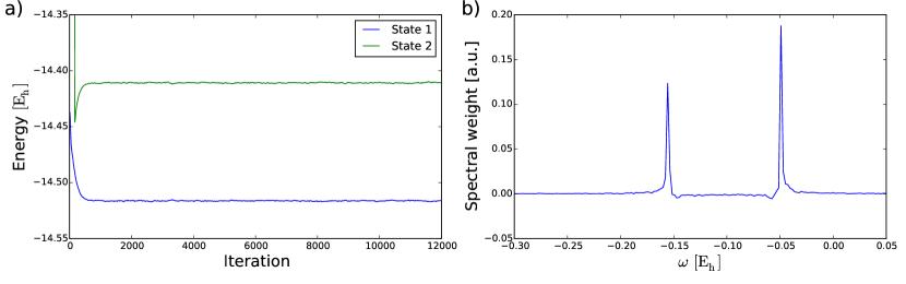
Figure 3: a) Energy over iteration for an excited state calculation with NECI for the Beryllium atom targeting two states in the $\mathrm{B_{1g}}$ irrep of the $D_{2h}$ symmetry group (corresponding to P-states). The two states have triplet/singlet character and the energy difference is $105.5\,\mathrm{mH}$. b) Spectral decomposition of a $2s\rightarrow 2p$ excited state of the Beryllium atom created using real-time evolution with NECI, containing the two lowest energy P-states which correspond to the states targeted in a). The gap between the two states is $106.6\,\mathrm{mH}$, agreeing with the excited state calculation within the spectral resolution of $2.1\,\mathrm{mH}$. The zero of the energy axis corresponds to the kation ground state energy. The output files are available in the supplementary material exc . In experiment, a value of $93.8\,\mathrm{mH}$ is observed for this energy gap Kramida and Martin (1997).

XI Transcorrelated Method

The computational cost of a Full CI method usually scales exponentially with respect to the size of the basis set. On the other hand, the low regularity of wave functions (characterized by the electronic cusp Kato (1957)) causes a very slow convergence towards the basis set limit. For calculations aiming at highly accurate results, it is very helpful to speed up such slow convergence.

A Jastrow AnsatzJastrow (1955) offers a way to factor out the cusp from the wave function

$$\ket{\Psi}=e^{\hat{T}}\ket{\Phi},$$ (25)

where $\hat{T}=\sum_{i<j}u({\bf r}_{i},{\bf r}_{j})$ is a symmetric function ($u({\bf r}_{i},{\bf r}_{j})=u({\bf r}_{j},{\bf r}_{i})$) over electron pairs, and $\ket{\Phi}$ is an anti-symmetric many-body function. By including the cusp term $|{\bf r}_{i}-{\bf r}_{j}|/2$ in $u({\bf r}_{i},{\bf r}_{j})$, the regularity of $\ket{\Phi}$ is improved at least by one order over $\ket{\Psi}$Fournais et al. (2009). We can also include other terms in $u({\bf r}_{i},{\bf r}_{j})$ to capture as much dynamic correlations as possible. By using variational quantum Monte Carlo methods (VMC), the pair correlation function $u({\bf r}_{i},{\bf r}_{j})$ can be obtained for a single determinant $\ket{\Phi}$ (e.g., $\ket{\Phi_{HF}}$) or a linear combination of small number of determinants (e.g., a small CAS wave function).

The transcorrelated method of Boys and Handy Boys and Handy (1969) provides a simple and efficient way to treat the Jastrow Ansatz, where the original Schrödinger equation is transformed into a non-Hermitian eigenvalue problem

$$\tilde{H}\ket{\Phi}=E\ket{\Phi},\quad\tilde{H}=e^{-\hat{T}}\hat{H}e^{\hat{T}}.$$ (26)

The advantage of this form of $\hat{T}$ is that the similarity transformation leads to an expansion which terminates at second order

$$\tilde{H} = \hat{H}+[\hat{H},\hat{T}]+\frac{1}{2}[[\hat{H},\hat{T}],\hat{T}]$$ (27)

$$= \hat{H}-\sum_{i}\left(\frac{1}{2}\nabla_{i}^{2}\hat{T}+(\nabla_{i}\hat{T})\nabla_{i}+\frac{1}{2}(\nabla_{i}\hat{T})^{2}\right)$$ (28)

$$= \hat{H}-\sum_{i<j}\hat{K}({\bf r}_{i},{\bf r}_{j})-\sum_{i<j<k}\hat{L}({\bf r}_{i},{\bf r}_{j},{\bf r}_{k}).$$ (29)

The similarity transformation introduces a novel two body operator $\hat{K}$ and a three-body potential $\hat{L}$

$$\hat{K}({\bf r}_{i},{\bf r}_{j}) = \frac{1}{2}\left(\nabla_{i}^{2}u({\bf r}_{i},{\bf r}_{j})+\nabla_{j}^{2}u({\bf r}_{i},{\bf r}_{j})+(\nabla_{i}u({\bf r}_{i},{\bf r}_{j}))^{2}+(\nabla_{j}u({\bf r}_{j},{\bf r}_{i}))^{2}\right)$$ (30)

$$+\left(\nabla_{i}u({\bf r}_{i},{\bf r}_{j}))\cdot\nabla_{i}+(\nabla_{j}u({\bf r}_{i},{\bf r}_{j}))\cdot\nabla_{j}\right)$$

$$\hat{L}({\bf r}_{i},{\bf r}_{j},{\bf r}_{k}) = \nabla_{i}u({\bf r}_{i},{\bf r}_{j})\cdot\nabla_{i}u({\bf r}_{i},{\bf r}_{k})+\nabla_{j}u({\bf r}_{j},{\bf r}_{i})\cdot\nabla_{j}u({\bf r}_{j},{\bf r}_{k})$$ (31)

$$+\nabla_{k}u({\bf r}_{k},{\bf r}_{i})\cdot\nabla_{k}u({\bf r}_{k},{\bf r}_{j}).$$

The whole transcorrelated Hamiltonian can be written in second quantised form as

$$\tilde{H} = \sum_{pq\sigma}h^{p}_{q}a^{\dagger}_{p\sigma}a_{q\sigma}+\frac{1}{2}\sum_{pqrs}(V^{pq}_{rs}-K^{pq}_{rs})\sum_{\sigma\tau}a^{\dagger}_{p\sigma}a^{\dagger}_{q\tau}a_{s\tau}a_{r\sigma}$$ (32)

$$-\frac{1}{6}\sum_{pqrstu}L^{pqr}_{stu}\sum_{\sigma\tau\lambda}a^{\dagger}_{p\sigma}a^{\dagger}_{q\tau}a^{\dagger}_{r\lambda}a_{u\lambda}a_{t\tau}a_{s\sigma},$$

where $h^{p}_{q}=\langle\phi_{p}|h|\phi_{q}\rangle$ and $V^{pq}_{rs}=\langle\phi_{p}\phi_{q}|r_{12}^{-1}|\phi_{r}\phi_{s}\rangle$ are the one- and two-body terms of the molecular Hamiltonian, while $K^{pq}_{rs}=\langle\phi_{p}\phi_{q}|\hat{K}|\phi_{r}\phi_{s}\rangle$ and $L^{pqr}_{stu}=\langle\phi_{p}\phi_{q}\phi_{r}|\hat{L}|\phi_{s}\phi_{t}\phi_{u}\rangle$ originate from the $\hat{K}$ and $\hat{L}$ operators.

This transcorrelated method has been investigated by FCIQMC using NECI , as it can essentially speed up the convergence with respect to basis sets. On the other hand the effective Hamiltonian is non-hermitian and contains up to three-body potentials. Luo and Alavi have explored a transcorrelated approach where only up to two-body potentials are involved Luo and Alavi (2018). The performance on uniform electron gases indicates this approach could be developed into an efficient FCIQMC method for plane wave basis sets in the future. For general molecular systems, the full transcorrelated Hamiltonian (32) is implemented in NECI , where $\hat{T}$ is fixed and treated as an input function, while $\ket{\Phi}$ is sampled by the FCIQMC algorithm. The lack of a lower bound of the energy due to the non-Hermiticity of the similarity transformed Hamiltonian poses a severe problem for variational approaches. However, as a projective technique, FCIQMC does not have an inherent problem sampling the ground-state right eigenvector by repetitive application of the projector (2) and obtaining the corresponding ground-state eigenvalue.

The matrix elements $K^{pq}_{rs}$ and $L^{pqr}_{stu}$ are pre-calculated and have to be supplied as input. The matrix elements of $K$ can be passed combined with the Coulomb integrals, while the matrix elements of $L$ are passed in a separate input file. This treatment is efficient for small atomic and molecular systems, but for large systems the storage of the $L$ matrix becomes a bottleneck. Here, efficient low rank tensor product expansion of $L$, might in the future make it practical to treat even larger systems. NECI supports storage of $L$ in a dense and a sparse format as well as on-the-fly calculation of $L^{pqr}_{stu}$ from a tensor decomposition. Additionally, major technical changes to the FCIQMC implementation are required for sampling up to triple excitations, which generally leads to reduced time-steps. The development of efficient excitation generation, which can alleviate the time-step bottleneck, is the subject of current work.

This method has been tested on the first row atoms Cohen et al. (2019), which shall serve as an example here. Two different correlation factors obtained by Schmidt and MoskowitzK. E. Schmidt and J. W. Moskowitz (1990) based on variance-minimisation VMC, which contain 7 and 17 terms of polynomial type basis functions have been employed there. The 7 term factor (SM7) contains mainly electron-electron correlation terms together with some electron-nuclear terms, while the 17 term factor (SM17) uses more terms to describe also the electron-electron-nuclear correlation. For the full CI expansion of $\ket{\Phi}$, three different basis sets, cc-pVDZ, cc-pVTZ and cc-pVQZ respectively have been used. In Fig. 4 the convergence of the total energies errors are displayed for the two different correlation factors, in comparison with the the CCSD(T)-F12 method. This demonstrates that improving the correlation factor can lead to a significant speed up of the basis set convergence. Using the 17 term factor, the CBS limit results can already be reached (within errors $<1$ mH) using a cc-pVQZ basis sets.

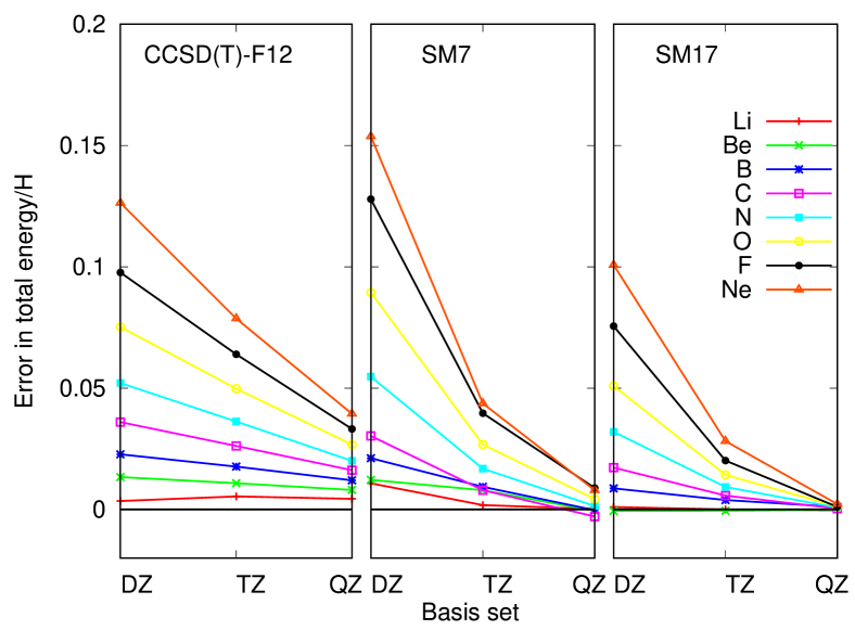
Figure 4: Exemplary application of the transcorrelated method: Errors in the total energies of the first-row atoms, in Hartree, for the two correlation functions and the F12 methodology. Reproduced from Cohen et al., JCP 151, 061101 (2019) Cohen et al. (2019) with the permission of AIP Publishing.

XII Symmetries and spin-adapted FCIQMC

Symmetry is a concept of paramount importance in the description and understanding of physical and chemical processes. According to Noether’s theorem there is a direct connection between conserved quantities of a system and its inherent symmetries. Thus, identifying them allows a deeper insight in the physical mechanisms of studied systems. Moreover, the usage of symmetries in electronic structure calculations enables a much more efficient formulation of the problem at hand. The Hamiltonian formulated in a basis respecting these symmetries has a block-diagonal structure, with zero overlap between states belonging to different ‘good’ quantum numbers. This greatly reduces the necessary computational effort to solve these problems and allows much larger systems to be studied.

XII.1 Common Symmetries utilized in Electronic Structure Calculations and NECI

There are several symmetries which are commonly used in electronic structure calculations, due to the above mentioned benefits and their ease of implementation. And our FCIQMC code NECI is no exception in this regard.

Conservation of the $\hat{S}_{z}$ spin-projection
As mentioned in section I, FCIQMC is usually formulated in a complete basis of Slater determinants (SDs). SDs are eigenfunctions of the total $\hat{S}_{z}$ operator, and consequently, if the studied Hamiltonian, $\hat{H}$, is spin-independent (no applied magnetic field and spin-orbit interaction) it commutes with $\hat{S}_{z}$, $[\hat{H},\hat{S}_{z}]=0$. The conservation of the $m_{s}$ eigenvalue in a FCIQMC calculation thus follows quite naturally: the initial chosen $m_{s}$ sector, determined by the starting SD used, will never be left by the random excitation generation process sketched in section II. No terms in the spin-conserving Hamiltonian will ever cause any state in the simulation to have a different $m_{s}$ value than the initial one. As a consequence the sampled wavefunction will always be an eigenfunction of $\hat{S}_{z}$ with a chosen $m_{s}$, determined at the start of a calculation.

Discrete and Point Group Symmetries in FCIQMC
NECI is also capable of utilizing Abelian point group symmetries, with D_2h being the ‘largest’ spatial group (similar to other quantum chemistry packages, e.g. MolcasAquilante et al. (2016) and MolproWerner et al. (2012a, 2015)), momentum conservation (due to translational invariance) in the Hubbard model and uniform electron gas calculations and preservation of the $m_{l}$ eigenvalues of the orbital angular momentum operator $\hat{L}_{z}$ (the underlying molecular orbitals have to be constructed as eigenfunction of $\hat{L}_{z}$). This is implemented via a symmetry-conserving excitation generation step and is explained in more detail in Appendix A.1.1.

XII.2 Total spin conservation

One important symmetry of spin-preserving, nonrelativistic Hamiltonians is the global $SU(2)$ spin-rotation symmetry. However, despite the theoretical benefits, the total $SU(2)$ spin symmetry is not as widely used as other symmetries, like translational or point group symmetries, due to their usually impractical and complicated implementation.

There are two kind of implementations of total spin conservation in our FCIQMC code NECI . One approximate one is based on Half-Projected Hartree-Fock (HPHF) functionsSmeyers and Doreste-Suarez (1973); Helgaker, Jørgensen, and Olsen (2000); Booth and Alavi et. al. (2013); Booth et al. (2011); Booth, Smart, and Alavi (2014). Their rationale relies on the fact that for an even number of electrons, every spin state $\ket{S}$ contains degenerate eigenfunctions with $m_{s}=0$. Using time-reversal symmetry arguments a HPHF function can be constructed as

$$\ket{H_{i}}=\begin{cases}\ket{D_{i}}&\text{for fully close-shell determinants}\\ \frac{1}{\sqrt{2}}\left(\ket{D_{i}}\pm\ket{\overline{D_{i}}}\right)&\text{otherwise,}\\ \end{cases}$$ (33)

where $\overline{\ket{D_{i}}}$ indicates the spin-flipped version of $\ket{D_{i}}$. Depending on the sign of the open-shell coupled determinants, $\ket{H_{i}}$ are eigenfunctions of $\hat{\mathbf{S}}^{2}$ with odd ($-$) or even ($+$) eigenvalue $S$. The use of HPHF is restricted to systems with an even number of electrons and can only target the lowest even- and odd-$S$ state. Thus, it can not differentiate between, e.g. a singlet $S=0$ and quintet $S=2$ state.

XII.2.1 The (graphical) Unitary Group Approach (GUGA)

Our full implementation of total spin conservation is based on the graphical Unitary group approach (GUGA). It relies on the observation that the spin-free excitation operators $\hat{E}_{ij}$ in the spin-free formulation of the electronic Hamiltonian,

$$\hat{H}=\sum_{ij}^{n}t_{ij}\hat{E}_{ij}+\sum_{ijkl}^{n}V_{ijkl}\left(\hat{E}_{ij}\hat{E}_{kl}-\delta_{jk}\hat{E}_{il}\right),$$ (34)

have the same commutation relations,

$$[\hat{E}_{ij},\hat{E}_{kl}]=\delta_{jk}\hat{E}_{il}-\delta_{il}\hat{E}_{kj},$$ (35)

as the generators of the Unitary group $U(n)$. This connection allows the usage of the Gel’fand-Tsetlin (GT) basisGel’fand and Cetlin (1950a, b); Gel’fand (1950), which is irreducible and invariant under the action of the operators $\hat{E}_{ij}$, in electronic structure calculations. The GT basis is a general basis for any irrep of $U(n)$, but PaldusPaldus (1974, 1975, 1976) realized that only a special subset is relevant for the electronic problem (34), due to the Pauli exclusion principle. Based on Paldus’ work, ShavittShavitt (1977) further developed an even more compact representation by introducing the graphical extension of the UGA. This leads to the most efficient encoding of a spin-adapted GT basis state (CSF) in form of a step-vector $\ket{\mathbf{d}}$. This step-vector representation has the same storage cost of two bits per spatial orbital as Slater determinants. The entries of this step-vector encode the change of the total number of electrons $\Delta N_{i}$ and the change of the total spin $\Delta S_{i}$ of subsequent spatial orbitals $i$. This is summarized in Table 1.

Table 1: Possible step-values $d_{i}$ and the corresponding change in number of electrons $\Delta N_{i}$ and total spin $\Delta S_{i}$ of subsequent spatial orbitals $i$.

$d_{i}$	$\Delta N_{i}$	$\Delta S_{i}$
0	0	0
1	1	-1/2
2	1	-1/2
3	2	0

All possible CSFs for a chosen number of spatial orbitals $N$, number of electrons $n$ and total spin $S$ are then given by all step-vectors $\ket{d}=\ket{d_{1},d_{2},\dots,d_{N}}$ fulfilling the restrictions

$$\sum_{i=1}^{N}\Delta n_{i}=n,\quad\sum_{i=1}^{N}\Delta S_{i}=S,\quad\text{and}\quad S_{k}=\sum_{i=1}^{k}\Delta S_{i}\geq 0.$$ (36)

The last restriction in Eq. 36 corresponds to the fact that the (intermediate) total spin must never be less than 0.

The most important finding of Paldus and ShavittShavitt (1978); Paldus (1981) was that the Hamiltonian matrix elements—more specifically the coupling coefficients between two CSFs, e.g. $\bra{m^{\prime}}\hat{E}_{ij}\ket{m}$—can be entirely formulated within the framework of the GUGA; without any reference and thus necessity to transform to a Slater determinant based formulation. Although CSFs can be expressed as a linear combination of SDs, the complexity of this transformation scales exponential with the number of open-shell orbitals of a specific CSFShavitt (1981). Thus, it is prohibitively hard to rely on such a transformation and for already more than $\approx 15$ electrons a formulation without any reference to SDs is much more preferable.

Furthermore, Shavitt and PaldusShavitt (1978); Paldus (1981) were able to find a very efficient formulation of the coupling coefficients as a product of terms, via the graphical extension of the UGA. Matrix elements between two given CSFs only depend on the shape of the loop enclosed by their graphical representation, as depicted in Fig. 5. The coupling coefficient of the one-body operator $\hat{E}_{ij}$ is given by

$$\bra{m^{\prime}}\hat{E}_{ij}\ket{m}=\prod_{k=i}^{j}W(Q_{k};d_{k}^{\prime},d_{k},\Delta S_{k},S_{k}),$$ (37)

where the product terms depend on the step-values of the two CSFs, $d_{k}^{\prime}$ and $d_{k}$, the difference in the current spin $\Delta S_{k}$ (with the restriction $S_{k}^{\prime}-S_{k}=\pm 1/2$) and the intermediate spin $S_{k}$ of $\ket{m}$ at orbital $k$. $Q_{k}$ in Eq. (37) depends on the shape of the loop formed by $\ket{m}$ and $\ket{m^{\prime}}$ at level $k$ and is tabulated in e.g. Ref. [Shavitt, 1978]. Additionally, the two CSFs, $\ket{m}$ and $\ket{m^{\prime}}$, must coincide outside the range $(i,j)$ for Eq. (37) to be non-zero.

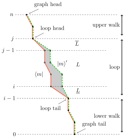
Figure 5: Graphical representation of the coupling coefficient between two CSFs, $\bra{m}\hat{E}_{ij}\ket{m^{\prime}}$.

XII.2.2 Spin-adapted excitation generation - GUGA-FCIQMC

The compact representation of spin-adapted basis functions in form of step-vectors and the product form of the coupling coefficients (37) allow for a very efficient implementation in our stochastic FCIQMC code NECI. As mentioned in Sec. II, the excitation generation step is at the heart of any FCIQMC code.

The main difference to a SD-based implementation of FCIQMC, apart from the more involved matrix element calculation (37), is the higher connectivity within a CSF basis. For a given excitation operator $\hat{E}_{ij}$, with spatial orbital indices $(i,j)$, there is usually more than one possible excited CSF $\ket{m^{\prime}}$ when applied to $\ket{m}$, $\hat{E}_{ij}\ket{m}=\sum_{k}c_{k}\ket{m^{\prime}_{k}}$. All valid spin-recouplings within the excitation range $(i,j)$ can have a non-zero coupling coefficient as well. This fact is usually the prohibiting factor in spin-adapted approaches. However, there is a quite virtuous combination of the concepts of FCIQMC and the GUGA formalism, as one only needs to pick one possible excitation from $\ket{m}$ to $\ket{m^{\prime}}$ in the excitation generation step of FCIQMC, see Sec. II.

We resolved this issue, by randomly choosing one possible valid branch in the graphical representation, depicted in Fig. 5, for randomly chosen spatial orbital indices $i,j(,k,l)$. Additionally we weight the random moves according to the expected magnitude of the coupling coefficientsDobrautz, Smart, and Alavi (2019); Dobrautz (2019) to ensure $p_{gen}(m^{\prime}|m)\propto|H_{m^{\prime}m}|$. This approach avoids the possible exponential scaling as a function of the open-shell orbitals of connected states within a CSF based approach.

However, this comes with the price of reduced generation probabilities and consequently a lower imaginary time-step, as mentioned in Sec. II. Combined with an additional effort of calculating these random choices in the excitation generation and the on-the-fly matrix element computation, the GUGA-FCIQMC implementation has a worse scaling with the number of spatial orbitals $N$ compared to a Slater determinant based implementationDobrautz, Smart, and Alavi (2019).

However, the benefits of using a spin-adapted basis are a reduced Hilbert space size, elimination of spin-contamination in the sampled wavefunction and most importantly: the spin-adapted FCIQMC implementation via the GUGA allows targeting specific spin states, which are otherwise not attainable with a SD based implementation as discussed in Ref. Dobrautz, Smart, and Alavi, 2019.

The unique specification of a target spin allows resolving near degenerate spin states and consequently numerical results can be interpreted more clearly. This enables more insight in the intricate interplay of nearly degenerate spin states and their effect on the chemical and physical properties of matter.

XII.2.3 Example: Hydrogen chain in a minimal basis

Figure 6: Schematic representation of a one-dimensional hydrogen chain of $L$ hydrogen atoms with equal separation $r$.

The GUGA-FCIQMC method has been benchmarked Dobrautz (2019) by applying it to a linear chain of $L$ equidistant hydrogen atoms Hachmann, Cardoen, and Chan (2006) recently studied to test a variety of quantum chemical methods Motta et al. (2017), which shall serve as an example here. Using a minimal STO-6G basis there is only one orbital per H atom and the system resembles a one-dimensional Hubbard model Hubbard (1963); Pariser and Parr (1953a, b); Gutzwiller (1963) with long-range interaction. Studying a system of hydrogen atoms removes complexities like core electrons or relativistic effects and thus is an convenient benchmark system for quantum chemical methods.

For large equidistant separation of the H atoms a localized basis, obtained with the default Boys-localization in Molpro’s LOCALI routine, with singly occupied orbitals centred at each hydrogen is more appropriate than a HF basis. Thus, this is an optimal difficult benchmark system of the GUGA-FCIQMC method, since the complexity of a spin-adapted basis depends on the number of open-shell orbitals, which is maximal for this system. Particularly targeting the low-spin eigenstates of such highly open-shell systems poses a difficult challenge within a spin-adapted formulation. This situation is depicted schematically in Fig. 6.

We studied this system to show that we are able to treat systems with up to 30 open-shell orbitals with our stochastic implementation of the GUGA approach Dobrautz (2019). We calculated the $S=0,1$ and $2$ (only $S=0$ for $L=30$) energy per atom up to $L=30$ H atoms in a minimal STO-6G basis at the stretched $r=3.6\,a_{0}$ geometryMotta et al. (2017) and compared it with DMRG Chan and Head-Gordon (2002); Sharma and Chan (2012); Chan and Sharma (2011); White (1992); Motta et al. (2017) reference results. The results are shown in Table 2, where we see excellent agreement within chemical accuracy with the reference results.

An important fact is the order of the orbitals though. Similar to the DMRG method it is most beneficial to order the orbitals according to their overlap, since the number of possible spin recouplings depends on the number of open shell orbitals in the excitation range. If we make a poor choice in the ordering of orbitals, excitations between physically adjacent and thus strongly overlapping orbitals are accompanied by numerous possible spin-recouplings in the excitation range, if stored far apart in the list of orbitals. This behaviour is thoroughly discussed in Ref [Li Manni, Dobrautz, and Alavi, 2020].

Table 2: Example for application of GUGA-FCIQMC: Difference of the energy per site $E/L$ of an hydrogen chain for different number $L$ of H atoms and total spin $S$ in a STO-6G basis set at the stretched bond distance of $r=3.6\,a_{0}$ compared with DMRG Chan and Head-Gordon (2002); Sharma and Chan (2012); Motta et al. (2017) reference resultsMotta et al. (2017). The GUGA-FCIQMC results were obtained without the initiator approximationCleland, Booth, and Alavi (2010). Reproduced from Dobrautz, Ph.D. thesis (2019) Dobrautz (2019).

L	S	$E_{ref}\,[E_{h}]$	$E_{FCIQMC}\,[E_{h}]$	$\Delta E\,[mE_{h}]$
20	0	-0.481979	-0.481978(1)0	-0.001(1)000
20	1	-0.481683	-0.481681(11)	-0.002(11)00
20	2	-0.480766	-0.480764(18)	-0.002(18)00
30	0	-0.482020	-0.481972(31)	-0.047(31)00

XIII Parallel scaling

When applying for access to large computing clusters, it is often necessary to demonstrate that the software being used (in this case NECI ) is capable of using the hardware efficiently. Ideally, the speed-up relative to using some base number of compute cores should grow perfectly linearly with the number of cores. In 2014, Booth et. al.Booth, Smart, and Alavi (2014), presented an example with 500$\times 10^{6}$ walkers in which no deviation from a linear speed-up is noticeable when comparing using 512 cores to using 32, and even at 2048 cores, a speed-up by a factor of 57.5 was reported, which is 90% of the ideal speed-up factor of 64. In that work, the largest number of cores explored was 2048. By comparing the performance for a calculation with 100$\times 10^{6}$ walkers and 500$\times 10^{6}$ walkers, the same figure showed that the speed-up became closer to the ideal speed-up when the number of walkers was increased, suggesting that when using even more walkers, the efficiency comes even closer to 100% of the ideal speed-up factor.

Since 90% of the ideal speed-up factor was achieved in 2014 with only 500$\times 10^{6}$ walkers on 2048 cores, and large compute clusters nowadays tend to have tens of thousands of cores available, we report scaling data for a much larger number of walkers on up to 24,800 cores in Table 4. The calculations were done using the integrals in FCIDUMP format for the (54e,54o) active space first described in Reiher et al. (2017) for the FeMoco molecule, and the output files are provided in the supplementary material sca .

The scaling analysis presented in Table 4 was done with 32 billion walkers on each of the two replicas used for the RDM sampling. Calculations at 32 billion walkers are expensive, so we only completed enough iterations to determine an accurate estimate of the average runtime per iteration for the scaling analysis, and not enough iterations to accurately estimate the energy.

One may ask whether or not the scaling observed in Table 4 was performed for a reasonable number of walkers for this active space. To answer this question, we compare in Table 3 the best (non-extrapolated) DMRG and sHCI-PT2 energies in the literature Li et al. (2019) to energies obtained with i-FCIQMC at only 8 billion walkers/replica, and find that the i-FCIQMC-RDM and i-FCIQMC-PT2 energies are closer together than the sHCI-VAR and sHCI-PT2 energies, indicating that the i-FCIQMC energies are closer to the true FCI limit where the difference between variational and PT2 energies should vanish. The DMRG result lies about half-way between the two i-FCIQMC results, but fairly well below the lower of the sHCI results (a forthcoming publication specifically about the FeMoco system is planned, in which more details will be presented, but the purpose of this paper is to give an overview of the NECI code).

Furthermore, comparing the time per iteration between $8\times 10^{9}$ and $32\times 10^{9}$ walkers shows that a high parallel efficiency is also achieved at the lower walker number. The determinants in NECI are stored using a hash table, making i-FCIQMC linearly scaling in the walker number Booth, Smart, and Alavi (2014), so the ideal time per iteration with $32\times 10^{9}$ walkers at 19960 cores according to the result for $8\times 10^{9}$ walkers at 16000 cores would be 23.4 seconds, which is only marginally smaller than the reported 23.5 seconds. Note however, that this is the relative efficiency between large scale calculations, which demonstrates performance gain from extending parallelization at large scales, not from parallelization over the entire range of scales, which is addressed to some extent by the Chromium dimer example below.

Table 3: Best non-extrapolated energies obtained for the CAS(54,54) of the FeMoco molecule, with three different methods. DMRG and sHCI energies were calculated in Ref. (Li et al., 2019), and i-FCIQMC results were obtained in this work with 8 billion walkers on each of the two replicas for the RDM sampling.

Method	Total Energy
i-FCIQMC-RDM	-13 482.	174 95(4)
i-FCIQMC-PT2	-13 482.	178 45(40)
sHCI-VAR	-13 482.	160 43
sHCI-PT2	-13 482.	173 38
DMRG	-13 482.	176 81

In the case of the Chromium dimer (cc-pVDZ, 28 electrons correlated in 76 spatial orbitals) considered in figure 7, the average time per iteration per walker ranges from $3.18\times 10^{-9}\,\mathrm{s}$ at 640 cores to $2.51\times 10^{-10}\,\mathrm{s}$ at 10240 cores and $1.53\times 10^{-10}\,\mathrm{s}$ at 20480 cores, corresponding to a parallel speed-up of 82.1% from 10240 to 20480 cores and an overall speed-up of 65.2% over the full range. The deviation from ideal scaling almost exclusively stems from the communication of the spawns, at lower walker numbers, the communicative overhead is more significant, reducing the parallel efficiency compared to the FeMoco example. Nevertheless, a very high yield can be obtained from scaling up the number of cores, even for already large scales.

XIII.1 Load balancing

The parallel efficiency of NECI is made possible by treating static load imbalance. NECI contains a load-balancing featureSpencer et al. (2019), which is enabled by default and periodically re-assigns some determinants to other processors in order to maintain a constant number of walkers per processor. As can be seen in figure  7, for the given benchmarks, no significant load imbalance occurs up to (including) 20480 cores loa ; fem . The initialization of a simulation does not feature the same speed-up due to I/O operations and initial communication such as trial wave function setup and core space generation. However, since it does not play a significant role for extended calculations, we consider only the time spent in the actual iterations.

# of walkers	# of cores	average time	ratio of	ratio of	efficiency of
		per iteration	# of cores	average time/iteration	parallelisation
$32\times 10^{9}$	19960	23.5 seconds	1.242	1.246	99.68%
$32\times 10^{9}$	24800	18.8 seconds
$8\times 10^{9}$	16000	7.3 seconds	-	-	-

Table 4: Efficiency of parallelisation for a CAS(54,54) of the FeMoco molecule. In both $32\times 10^{9}$ walkers cases, the time per iteration is averaged over more than 250 iterations and in both cases the unbiased sample variance over the 250+ iterations is less than 0.5 seconds. For comparison, the time per iteration for $8\times 10^{9}$ walkers which was used to obtain the energy reported in table 3, is given. Calculations were run on 512, 620 and 400 nodes with Intel Xeon Gold 6148 Skylake processors with 20 cores at 2.4 GHz and 96 GB of DDR4 RAM, and all nodes were in a single island with a 100 Gb/s OmniPath interconnect between the nodes. Hyperthreading was not used.

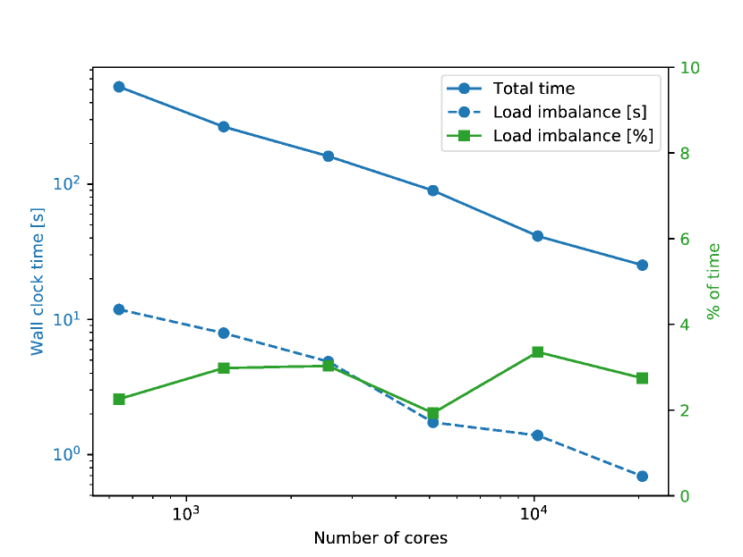
Figure 7: Total time and time lost due to load imbalance for running 100 iterations with 1.6 Billion walkers for the Cr₂/cc-pVDZ (28e in 76o) on 640 to 20480 cores (not counting initialisation). The calculations were run on Intel Xeon Gold 6148 Skylake processors, with a 100 Gb/s OmniPath node interconnect. The code was compiled using the Intel Fortran compiler, version 19.0.4. A semi-stochastic core-space of 50000 determinants was used, and PCHB excitation generation. For the largest number of cores, the time step is $3.68\times 10^{-4}$ with an average acceptance ratio of 12.51%, which is representative for all numbers of cores. The load imbalance time is measured as the accumulated difference between the maximum and average time per iteration across MPI tasks. Figure generated using Matplotlib Hunter (2007).

XIV Interfacing NECI

The ongoing development of NECI is focused on an efficiently scaling solver for the CI-problem. It is not desirable to reimplement functionality that is already available in existing quantum chemistry codes. Since the CI-problem is defined by the electronic integrals and subsequent methods depend on the results of the CI-step, namely the reduced density matrices, it is easily possible to replace a CI-solver of existing quantum chemistry code with NECI .

To use NECI only an input file and a FCIDUMP file Knowles and Handy (1989), which is the widely understood file format for the electronic integrals, are required. After running NECI the stochastically sampled reduced density matrices are available as input for further calculations in other codes. It is possible to link NECI as library and call it directly or to run it as external process and do the communication with explicit copying of files. The first alternative will be referred to as embedded, the second is the decoupled form.

Due to the stochastic nature of the Monte Carlo algorithm, it is not yet possible to use NECI as a black box CI-solver for larger systems. In this case it is recommended to use the decoupled form for a better manual control of the convergence. Another advantage of the decoupled form is the combination of NECI with different quantum chemical algorithms or implementations that do not benefit from massive parallelisation as much as NECI . This way it is possible to switch from serial or single node execution to multiple nodes in the CI-step. So far NECI has been coupled with Molpro  Werner et al. (2012b, 2019), Molcas 8Aquilante et al. (2016), OpenMolcas  Fdez. Galván et al. (2019), PySCF  Sun et al. (2017), and VASP  Kresse and Furthmüller (1996).

XV Stochastic-MCSCF

The Stochastic multi-configurational self-consistent field (MCSCF) procedure emerges from the combination of conventional MCSCF methodologies with FCIQMC as the CI-eigensolver. Stochastic-MCSCF approaches greatly enlarge the applicability of FCIQMC to strongly correlated molecular systems of practical interest in chemical science.

To date two implementations of Stochastic-MCSCF have been made available, based on the interface of NECI with OpenMolcas  Li Manni, Smart, and Alavi (2016); Fdez. Galván et al. (2019) (and Molcas 8 Aquilante et al. (2016)) and PySCF  Thomas et al. (2015a); Sun et al. (2017). As they are both based on the complete active space (CAS) concept, they are often also referred to as Stochastic-CASSCF methods.

The Stochastic-CASSCF implemented in PySCF is based on a second order CASSCF algorithm Sun, Yang, and Chan (2017) which decouples the orbital optimization problem from the active space CI problem, allowing for easy interfacing with NECI .

At each macro-iteration, a FCIQMC simulation is performed at the current point of orbital expansion, and density matrices are stochastically sampled (see section VII). These are then passed back to PySCF, which updates the orbital coefficients accordingly, using either a 1-stepSun, Yang, and Chan (2017) or 2-step approachYanai et al. (2009).

The Stochastic-CASSCF implemented in OpenMolcas is based on the quasi-second order Super-CI orbital optimization. Optimal orbitals (in the variational sense) are found by solving the Super-CI secular equations in the $\ket{\text{Super}-CI}$ basis, defined by the CAS wave function at the point of expansion, $|0\rangle$, and all its possible single excitations

$$|\text{Super}-CI\rangle=|0\rangle+\sum_{p>q}{\chi_{pq}(\hat{E}_{pq}-\hat{E}_{qp})|0\rangle}$$ (38)

The wave function is improved by mixing single excitations to the $|0\rangle$ wave function. As the CASSCF optimization proceeds, the $\chi_{pq}$ coefficients decrease until they vanish, and $|0\rangle$ will reveal the variational stationary point. Third-order density matrix elements of the exact Super-CI approach are avoided by utilizing an effective one-electron Hamiltonian, as discussed in greater details in Reference 19.

A flow chart of Stochastic-CASSCF describing the various steps of the CASSCF wave function optimization is given in Figure 8.

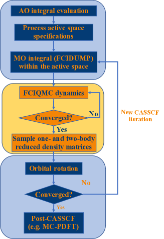
Figure 8: Flow chart summarizing the Stochastic-CASSCF steps. The blue boxes represent parts of the algorithm performed at the OpenMolcas or PySCF interfacing software. The center yellow box shows the two crucial FCIQMC steps, stochastic optimization of the CAS-CI wave function and sampling of one- and two-body reduced density matrices. When embedded schemes are employed, additional external potentials are added within the interfacing software when generating the FCIDUMP file. Post-CASSCF procedures, such as the MC-PDFT methodology, follow the Stochastic-CASSCF approach within the interfacing software.

The Stochastic-CASSCF approach has successfully been applied to a number of challenging chemical problems. The accuracy of the method has been demonstrated on simple test cases, such as benzene and naphthalene Thomas et al. (2015a) and more complex molecular systems, namely coronene Thomas et al. (2015a), free-base porphyrin and Mg-porphyrin Li Manni, Smart, and Alavi (2016). More recently the method has also been applied to understand the mechanism stabilizing intermediate spin states in Fe(II)-porphyrin Li Manni and Alavi (2018); Li Manni et al. (2019), the study of a $[Fe(III)_{2}S_{2}(SCH_{3})_{2}]^{2-}$ iron-sulfur model system in its oxidized form Li Manni, Dobrautz, and Alavi (2020), and new superexchange paths in corner-sharing cuprates Bogdanov et al. (2018).

To date, only state specific Stochastic-CASSCF optimizations have been reported. However, state-average Stochastic-CASSCF optimizations are a straightforward extension that can be reached by taking advantage of the NECI capability to optimize excited states wave functions, as discussed in section VIII. The Stochastic-CASSCF method can also be coupled to the adaptive shift approach discussed in section V with a great enhancement in performance.

XVI Conclusion

With NECI we present a state of the art FCIQMC program capable of running a large variety of versions of the FCIQMC algorithm. This includes the semi-stochastic FCIQMC feature, energy estimation using trial wave functions, the stochastic sampling of reduced density matrices, and excited state calculations. Further features of NECI’s FCIQMC implementation discussed are the real-time FCIQMC method and the adaptive shift method, as well as a spin-adapted formulation of the algorithm and support for transcorrelated Hamiltonians. We demonstrated the scalability of the program to up to 24800 cores, showing that the code can run efficiently on large-scale machines.

Finally, we highlighted the interoperability of NECI with other quantum chemistry software, in particular OpenMolcas and PySCF , which can be used to run Stochastic-CASSCF calculations.

XVII Supplementary Materials

Example FCIQMC output files for excited state calculations ( output_file_excited_state_be2_b1g.txt and stats_file_excited_state_be2_b1g.txt) and real-time calculations including the resulting spectrum (output_file_real_time_be2_b1g.txt, and fft_spectrum_be2_b1g.txt) for the examples presented in section 3 are available in the supplemental material. Furthermore, the supplement contains the output files for scaling (output_file_scaling_with_*_cores.txt and output_file_energy_with_8b_walkers.txt) and load imbalance analysis (output_file_load_imbalance_n*.txt). Exemplary output and integral files for a similarity transformed FCIQMC calculation of the Neon atom in a cc-pVDZ basis set are also supplied in the supplement (tcdump_Ne_st_pVDZ.h5 and FCIDUMP_Ne_st_pVDZ integral files and output_file_Ne_st_pVDZ.txt output stats_file_Ne_st_pVDZ.txt files). All output files contain the corresponding FCIQMC input.

XVIII Data availability statement

The data that supports the findings of this study are available within the article and its supplementary material sup . The NECI program can be obtained at https://github.com/ghb24/NECI_STABLE, the development version can be obtained from the corresponding author upon reasonable request.

Appendix A Stochastic excitation generation and $p_{gen}$

In the following appendices we will consider in some detail the process of (random) excitation generation in FCIQMC - a crucial yet rather flexible aspect of the algorithm. We will consider some general aspects, such as implementation of Abelian symmetries in the excitation process, as well as non-uniform excitation generation, as is often desirable in quantum chemical Hamiltonians. There are other classes of systems (such as Hubbard models, Transcorrelated Hamiltonians, spin models such as Heisenberg systems, etc) for which more specialised considerations are necessary for efficient excitation generation but we will not consider them here.

The first general point about excitation generation, (by which we mean starting from a given determinant $\ket{D_{i}}$ we randomly pick either one or two electrons, and a corresponding number of holes to substitute them with, to create a second determinant $\ket{D_{j}}$), is that if $|H_{ij}|>0$, then the probability ($p_{gen}(j|i)$) to select $\ket{D_{j}}$ and $\ket{D_{i}}$, must also be greater than 0. Furthermore, $p_{gen}(j|i)$ must be computable, and in general the effort to do so will depend on the algorithm chosen to execute the excitation process.

Let us discuss in more detail the process of stochastic excitation generation, and its impact on $p_{gen}$. Suppose we are simulating a system of $n$ electrons in $2N$ spin orbitals $\{\phi_{1},...,\phi_{2N}\}$. A given determinant $\ket{D_{i}}$ can be defined by its occupation number representation, $I=\ket{n_{1},...,n_{2N}}$, which is a binary string such that $n_{i}=1$ if orbital $i$ is occupied (‘an electron in $\ket{D_{i}}$’), and $n_{i}=0$ if it is unoccupied (‘a hole in $\ket{D_{i}}$’). Each orbital carries a spin quantum number $\sigma(\phi_{i})$, and may also carry a symmetry label, $\Gamma(\phi_{i})$. These are both discrete symmetries, with $\sigma=\pm 1/2$, and $\Gamma=\Gamma_{1},...,\Gamma_{G}$, where $G$ is the number of irreducible representations available in the point-group of system under consideration. We will only consider Abelian groups, so that the product of symmetry labels uniquely specifies another symmetry label. This simplifies the task of selecting excitations, although it does not necessarily exploit the full symmetry of the problem.

A.1 Uniform excitation generation

Now we wish to perform a stochastic excitation generation, which we will initially consider without the use of any symmetry/spin information. For example, we can select a pair of electrons, $i,j$ (with $i<j$) in $\ket{D_{i}}$, at random, and a pair of holes $a,b$ (with $a<b$), and perform the transition $ij\rightarrow ab$. The corresponding matrix element is

$$H_{ij}^{ab}=\braket{ij}{ab}-\braket{ij}{ba}\equiv\braket{ij}{ab}$$ (39)

We will denote the electron pair simply as $ij$ and the hole pair $ab$.

For this simple procedure, it is clear that the probability to choose $\ket{D_{j}}$ from $\ket{D_{i}}$ is simply:

$$p_{gen}(j|i)={n\choose 2}^{-1}{2N-n\choose 2}^{-1}$$ (40)

from which it follows that $p_{gen}(j|i)\sim(nN)^{-2}$. This procedure does not take symmetry or spin quantum numbers into account, and it is quite possible that the corresponding Hamiltonian matrix element is zero. To ensure that we do not generate such excitations, we need to select the hole pairs so that following two conditions are met:

$$\sigma(\phi_{i})+\sigma(\phi_{j}) = \sigma(\phi_{a})+\sigma(\phi_{b}),$$ (41)

$$\Gamma(\phi_{i})\times\Gamma(\phi_{j}) = \Gamma(\phi_{a})\times\Gamma(\phi_{b}).$$ (42)

These restriction greatly impact the way in which we will select $i,j$ and $a,b$, and the resulting generation probability.

A.1.1 Imposing symmetries via conditional probabilities

One way to impose symmetries in excitation generation while keeping track of the generation probabilities is via the notion of conditional probabilities. For example, rather than drawing $(ij)$ and $(ab)$ independently, with probability $p(ab,ij)=p(ab)p(ij)$, one can instead draw $(ab)$ given that one has already drawn $(ij)$; the probability for this process is given by

$$p(ab,ij)=p(ab|ij)p(ij),$$ (43)

where $p(ij)$ is the probability to select $(ij)$ in the first place. If $(ij)$ has a particular characteristic that confers a physical (e.g. symmetry-related) constraint on $(ab)$, this can be implemented at the stage in which we select $(ab)$: $(ab)$ need only be selected from among those hole-pairs for which the constraint is satisfied. For example, if the electrons $(ij)$ have opposite spins then the holes $(ab)$ must also have opposite spins. The smaller number of possibilities in choosing the $ab$ pair then leads to a larger $p(ab|ij)$ compared to $p(ab)$, which can be thought of as a renormalisation of the latter probability to take into account the constraint.

The concept of conditional probabilities can be further extended so that the pair $(ij)$ itself is made to satisfy a particular condition. Suppose we introduce a set of of conditions $\{{\cal{C}}_{1},{\cal{C}}_{2},...\}$ such that the union of all such conditions is exhaustive. It is possible to draw conditional probabilities with respect to such conditions. For example,

$${\cal{C}}_{1} =$$ ‘electron pair have the same spin’ (44)

$${\cal{C}}_{2} =$$ ‘electron pair have opposite spins’ (45)

then one can write:

$$p(ab,ij)=p(ab,ij|{\cal{C}}_{1})p({\cal{C}}_{1})+p(ab,ij|{\cal{C}}_{2})p({\cal{C}}_{2})$$ (46)

with

$$p({\cal{C}}_{1})+p({\cal{C}}_{2})=1.$$ (47)

$p({\cal{C}}_{1})$, the probability to select same-spin excitations, can be chosen arbitrarily, which then fixes $p({\cal{C}}_{2})$ according to the above.

The advantage of this formulation is that we can skew the selection of electron pairs, for example, towards opposite spin excitations if that proves advantageous, and to be able to compute the resulting probabilities. Furthermore, we can write:

$$p(ab,ij|{\cal{C}}_{1})=p(ab|ij)p(ij|{\cal{C}}_{1})$$ (48)

$$p(ab,ij|{\cal{C}}_{2})=p(ab|ij)p(ij|{\cal{C}}_{2})$$ (49)

which allows us to select a pair of electrons satisfying condition ${\cal{C}}_{1}$, and subsequently draw a pair of holes given one has selected an electron pair with the same spin (which implies that hole-pair must be chosen to have the same spin as the electron-pair).

A.2 Cauchy-Schwartz excitation generation

Let us now consider how to generate the hole pairs in a non-uniform manner, to reflect the fact that, in ab initio Hamiltonians, the matrix elements vary strongly in magnitude. Since the spawning probability is proportional to the ratio $\lvert H_{ij}\rvert/p_{\mathrm{gen}}(j|i)$, it is clearly desirable to generate excitations which make this ratio as uniform as possible, ideally with $p_{\mathrm{gen}}(j|i)\propto|H_{ij}|$. In this way, one would ensure a relatively uniform probability of successful spawning, which ideally would be close to one, implying a low rejection rate. Keeping the discussion focussed on double excitations (the generalisation to single excitations being straightforward) the question that arises is: how best can one select $ij$ and $ab$ such that $p_{\mathrm{gen}}(j|i)\propto\lvert H_{ij}\rvert$ to a good approximation, and $p_{gen}$ remains exactly computable without excessive cost. We will see there is a compromise to be made. One can ensure precise proportionality between $p_{\mathrm{gen}}(j|i)$ and $\lvert H_{ij}\rvert$ but only at prohibitive cost. Alternatively, one might be able to select $ij$ and $ab$ to effect the transition $\ket{D_{i}}\rightarrow\ket{D_{j}}$ based on computationally inexpensive heuristics, to provide approximate proportionality, which will nevertheless allow for a large overall improvement in efficiency.

To ensure exact proportionality between $p_{\mathrm{gen}}(j|i)$ and $\lvert H_{ij}\rvert$ it is necessary to enumerate all electron-pairs and hole-pairs which are possible from $\ket{D_{i}}$, and to construct the cumulative probability function (CPF), from which the desired distribution can be straightforwardly sampled. The (unnormalised) CPF is:

$$F_{ab,ij}[D]=\sum_{ee^{\prime}\in D}^{ij}\sum_{hh^{\prime}\in D}^{ab}\lvert\braket{ee^{\prime}}{hh^{\prime}}\rvert$$ (50)

In this expression, the sum over $ee^{\prime}$ runs over all enumerated electron pairs in $D$ up to $ij$, and similarly for the hole-pairs (up to $ab$). The CPF is a non-decreasing function of its discrete arguments, and its inverse transform enables one to select $ab$ and $ij$ with probability proportional to $\lvert\braket{ij}{ab}\rvert$. From the point of generation probabilities, this is the ideal excitation generator, allowing for a uniform spawning probability (which can be made to equal unity, implying zero rejection rates.) Unfortunately the CPF costs $\mathcal{O}(n^{2}N^{2})$ to set up (for each determinant $\ket{D_{i}}$), making it prohibitive in practice.

To make practical progress, we need an approximate distribution function which is much cheaper to calculate. Two observations can be made in this relation. First, if the two electrons have different spin, then the Hamiltonian matrix element consists of only one rather than two terms. This is because upon excitation $ij\rightarrow ab$, the two holes must match the spins of the two electrons. For example $\sigma(a)=\sigma(i)$ and $\sigma(b)=\sigma(j)$. In this case, the Hamiltonian matrix element reduces to:

$$H_{ij}=\braket{ij}{ab}$$ (51)

with the exchange term $\braket{ij}{ba}=0$.

With this simpler matrix element, we now ask: given that we have chosen an electron pair $ij$, how can we select the hole pair $ab$ so that, with high probability, the resulting matrix element $\braket{ij}{ab}$ is large? At this point we can appeal to the Cauchy-Schwarz inequality, which provides a strict upper bound:

$$\braket{ij}{ab}\leq\sqrt{\braket{ii}{aa}\braket{jj}{bb}}$$ (52)

This suggests that, as long as $\braket{ij}{ab}$ is non-zero by symmetry, it may be advantageous to select the hole $a$ so that $\braket{ii}{aa}$ is large, and the hole $b$ so that $\braket{jj}{bb}$ large. Because $i$ and $j$ have different spins, the selection of $a$ and $b$ will be independent of each other, with $a$ for example being chosen from the $\alpha$-spin holes available, and $b$ from the $\beta$-spin holes. To do this, we set up two CPFs:

$$F_{a}[i\in\alpha D] = \sum_{h\in\alpha D}^{a}\sqrt{\braket{hh}{ii}},$$ (53)

$$F_{b}[j\in\beta D] = \sum_{h\in\beta D}^{b}\sqrt{\braket{hh}{jj}},$$ (54)

where the sums over $h$ runs over the $\alpha$ or $\beta$ holes in $D$. (The notation $i\in\alpha D$ means an $\alpha$-electron in $D$, and $h\in\alpha D$ means an $\alpha$-hole in $D$). Unlike Eq.(50), these CPFs cost only $\mathcal{O}(N)$ to set up, and allow (via their inverse transforms) the selection of $a$ and $b$ with probabilities proportional to $\sqrt{\braket{aa}{ii}}$ and $\sqrt{\braket{jj}{bb}}$ respectively.

The Cauchy-Schwarz bound on an individual 4-index integral provides a very useful factorised approximation for the purposes of excitation generation, especially for opposite-spin excitations. The case for same-spin excitations is less favourable because it involves the difference between two 4-index integrals, and in this case we must obtain an upper bound for this difference expressed in a factorised form. We use the following much less tight upper bound:

$$\lvert\braket{ij}{ab}-\braket{ij}{ba}\rvert \leq[\sqrt{\braket{aa}{ii}}+\sqrt{\braket{aa}{jj}}]$$ (55)

$$\times[\sqrt{\braket{bb}{ii}}+\sqrt{\braket{bb}{jj}}]$$ (56)

In practice, we must draw two holes $a$ and $b$ from the same set of holes, avoiding the possibility of drawing the same hole twice. Because we would like to avoid setting up a two-dimensional CPF (which would cost $\mathcal{O}(N^{2})$), we create one one-dimension CPF in order to draw hole $a$, and then remove this hole in the CPF before drawing the second hole. In other words we set up two related CPFs

$$F_{a}[ij\in D] = \sum_{h}^{a}\sqrt{\braket{ii}{hh}}+\sqrt{\braket{jj}{hh}},$$ (57)

$$F^{\prime}_{b}[ij\in D] = \begin{cases}F_{b}[ij\in D|a]&\text{if}\;b<a,\\ \begin{aligned} &F_{b}[ij\in D]-\sqrt{\braket{ii}{aa}}\\ &\;\;\;-\sqrt{\braket{jj}{aa}}\end{aligned}&\mathrm{if}\;b\geq a,\end{cases}$$ (58)

drawing hole $a$ from $F_{a}$ and hole $b$ from $F^{\prime}_{b}$.

Our exploration of excitation generation has led us to discover many highly performing schemes. The Cauchy-Schwarz (CS) scheme presented above is a good starting point, but it has a number of weaknesses that can be further addressed. In particular, as noted above, the upper bound obtained is particularly poor for double excitations with the same spin, and in general the specified bound can be too loose. Fortunately, the selection of the second hole, $b$, is made once the first hole, $a$, has already been chosen, and as such the exact double excitation Hamiltonian matrix elements can be used at this stage, such that an updated CPF for selecting the second electron is given by

$$F_{b}[ij\in D|a]=\sum_{\begin{subarray}{c}h\in D\\ h\neq a\end{subarray}}^{b}\sqrt{\lvert\braket{ij}{ab}-\braket{ij}{ba}\rvert}.$$ (59)

This Part-Exact (PE) scheme no longer provides a strict bound, but by better representing the cancellation of terms present in these matrix elements, it provides a substantially better approximation. More crucially, it improves the prediction of the elements that were previously handled least effectively, and thus relaxes the time-step constraints on the overall calculation.

Due to the increase in computational cost involved in constructing two lists, and the additional normalisation of the probabilities required by causing the two selections not to be made in the same manner, this update to the scheme increases computational cost per iteration. In almost all systems examined this is far outweighed by the time-step changes, especially in systems with large basis sets or with translational symmetry. However, it is possible to find systems where the pure CS scheme is more optimal.

A.2.1 Preparing for excitation generation

For determinant $D$, to pick an excited determinant, first construct a table of hole occupancies for each spin and irreducible representation, so that $n_{\sigma\Gamma}[D]$ is the number of holes with spin $\sigma$ in irrep $\Gamma$ available in $D$. This is an $\mathcal{O}(n)$ process.

We next decide whether we wish to make a single excitation or a double excitation from $D$. A single excitation is chosen with probability $p_{sing}$, a parameter which can be optimised as the simulation proceeds to maximise the acceptance ratio and time-step of the simulation. The probability to create a double excitation is chosen such that the maximal ratios $\frac{|H_{ij}|}{p_{gen}(j|i)}$ for single and double excitations are equal, which for ab initio systems typically means double excitations dominate. To a first approximation $p_{sing}=nN/(nN+n^{2}N^{2})$, which is in general a small number on the order of $(nN)^{-1}$. The probability of attempting a double excitation is then $p_{doub}=1-p_{sing}$.

A.2.2 Single Excitations

If a single excitation is being attempted, first select an electron (say $i$) at random, with probability $n^{-1}$. The spin $\sigma=\sigma(i)$ and irrep $\Gamma=\Gamma(\phi_{i})$ of the electron determines the spin and irrep of the hole.

To select the hole $a$, run over all $n_{\sigma\Gamma}$ holes available in $D$ with spin and symmetry $\sigma\Gamma$, and compute the (unnormalised) cumulative probability function,

$$F^{(1)}_{a}[i\in D]=\sum_{h\in\sigma\Gamma D}^{a}|\braket{D_{i}^{h}}{\hat{H}}{D}|,$$ (60)

where $\ket{D_{i}^{h}}$ is a single-excitation $i\rightarrow h$ from $\ket{D}$, and $\braket{D_{i}^{h}}{\hat{H}}{D}$ is the Hamiltonian matrix element between them. The normalisation of the CPF is give by the last element in the array:

$$\Sigma_{i}=F^{(1)}_{n_{\sigma\Gamma}}[i\in D],$$ (61)

where $n_{\sigma\Gamma}$ is the number of holes available with spin $\sigma$ in irrep $\Gamma$ in $D$. Using $F^{(1)}_{a}$, select hole $a$ (with probability $|\langle D_{i}^{a}|H|D\rangle|$), by inverting the CPF. This is selected by generating a uniform random number $\xi$ in the interval $[0,\Sigma_{i})$, and determining the index of $a$ such that the condition

$$F^{(1)}_{a-1}<\xi\leq F^{(1)}_{a}$$ (62)

is met. The overall generation probability for this excitation is:

$$p_{gen}(a,i)=p(a|i)\times p(i)\times p_{sing},$$ (63)

where

$$p(a|i) =\frac{\theta_{a}}{\Sigma_{i}},$$ (64)

$$\theta_{a} =F^{(1)}_{a}-F^{(1)}_{a-1},$$ (65)

$$p(i) =n^{-1}.$$ (66)

This completes the selection of a singly excited determinant. The computation of $F^{(1)}_{a}$ is an order $\mathcal{O}(nN)$ operation (with $\mathcal{O}(N)$ holes being summed over, and each Hamiltonian matrix element being $\mathcal{O}(n)$ to compute). Although this is expensive, the generation of single excitations turns out overall to be a small fraction of the total cost, largely because the relatively small number of times such excitations are attempted.

A.2.3 Double Excitations with opposite spin electron-pairs

If a double excitation is being attempted, then firstly a pair of electrons needs to be selected. The first electron, $i$, should be selected uniformly at random. Following this, the CPF

$$F_{j}[i\in D]=\sum_{\begin{subarray}{c}k\in D\\ k\neq i\end{subarray}}^{j}\braket{ik}{ik}\times\begin{cases}p_{opp}&\text{if $i,k$ opp},\\ 1-p_{opp}&\text{otherwise.}\end{cases}$$ (67)

should be constructed, where $p_{opp}$ is a optimisable biasing factor towards excitations with electrons having opposite spins. The second electron is selected through inversion of the CPF.

If the two selected electrons have opposite spins, then the first hole to be chosen is, by convention, always a $\beta$ electron, and the second hole always $\alpha$. This choice is entirely arbitrary, and in some high-spin systems it may make sense to reverse this selection. Considering all available orbitals of this spin, the CPF

$$F^{(\beta)}_{a}[i\in D]=\sum_{h\in\beta D}^{a}\sqrt{\braket{hh}{ii}},$$ (68)

is constructed, where $i$ is taken to be the electron from the selected pair with $\beta$ spin, and the hole selected by inverting the CPF.

Once this first electron has been chosen, the symmetry of the target orbital is now fixed by the constraint that $\Gamma_{a}\otimes\Gamma^{\prime}=\Gamma_{i}\otimes\Gamma_{j}$. This greatly restricts the number of holes that must be considered when constructing the final CPF,

$$F^{(\alpha\Gamma^{\prime}a)}_{b}[ij\in D]=\sum_{h\in\alpha\Gamma^{\prime}D}^{b}\sqrt{\lvert\braket{ij}{ab}\rvert}.$$ (69)

Note that with the conventional choice of orbital $i$ above, $\braket{ji}{ah}=0$, and can thus be excluded. The second hole is then also obtained by inverting the CPF. The generation probability is then given by:

$$p_{gen}(ab,ij) =p(ij)p(a|i)p(b|ija)p_{doub},$$ (70)

$$p(ij) =\frac{1}{N}\left(\frac{\theta_{j}^{(i)}}{\Sigma_{i}}+\frac{\theta^{(j)}_{i}}{\Sigma_{j}}\right),$$ (71)

$$\theta_{j}^{(i)} =F_{j}[i\in D]-F_{j-i}[i\in D],$$ (72)

$$p(a|i) =\frac{\theta_{a}}{\Sigma^{(\beta)}(i)},$$ (73)

$$\theta_{a} =F^{(\beta)}_{a}-F^{(\beta)}_{a-1},$$ (74)

$$p(b|ija) =\frac{\theta_{b}}{\Sigma^{(\alpha\Gamma^{\prime})}(ija)},$$ (75)

$$\theta_{b} =F^{(\alpha\Gamma^{\prime}a)}_{b}-F^{(\alpha\Gamma^{\prime}a)}_{b-1},$$ (76)

where $\Sigma_{i},\Sigma^{(\beta)}(i),\Sigma^{(\alpha\Gamma^{\prime})}(ija)$ are the normalisations of $F_{j},F^{(\beta)}_{a},F^{(\alpha\Gamma^{\prime}a)}_{b}$ respectively, and are given by the final entries of the corresponding arrays.

The asymetric selection of $\alpha$ and $\beta$ holes is somewhat peculiar. It should be noted that it is possible to make this selection symmetrically, considering all available holes in the selection of the first hole, and then renormalising the probabilities to account for the possibility of selecting $b$ first. The symmetric scheme increases computational cost substantially (twice as many holes need to be considered in the CPF, and a further CPF must be calculated for the renormalisation). It also makes the overall time-step behaviour worse as, although it improves the general smoothness, for the worst-case scenario with a very rarely selected excitation with very different $a,b$ and $b,a$ probabilities, the denominator is increased substantially by considering more orbitals, whilst leaving the numerator essentially unchanged.

A.2.4 Double excitations with same-spin electron pairs

If the pair of electrons, selected as described above, have the same spin the process needs to account for the fact that the holes can be selected in either order, and the probabilities need to be adjusted to compensate.

Now, considering only holes with the same spin as the two electrons, construct the CPF

$$F_{a}^{(\sigma)}[ij\in D]=\sum_{h\in\sigma D}^{a}\sqrt{\braket{hh}{ii}}+\sqrt{\braket{hh}{jj}}.$$ (77)

Hole $a$ can then be selected through inversion of this CPF, which fixes the symmetry of hole $b$ such that $\Gamma_{a}\otimes\Gamma_{b}=\Gamma_{i}\otimes\Gamma_{j}$. The CPF for selecting the second hole can then be constructed from the (much smaller) set of holes with the appropriate symmetry, such that

$$F^{(\sigma\Gamma_{b}a)}_{b}[ij\in D]=\sum_{\begin{subarray}{c}h\in\alpha\Gamma_{b}D\\ h\neq a\end{subarray}}^{b}\sqrt{\lvert\braket{ij}{ab}-\braket{ij}{ba}\rvert}.$$ (78)

The second hole, $b$, can then be selected through inversion of this CPF. It is important to note that as the selection of the first hole includes all holes of the hole with the given spin, the selection of the holes could have been made in the reverse order, and this needs to be taken into account in the generation probability, which is given by:

$$p_{gen}(ab,ij)=[p(a|ijb)p(b|ij)+p(b|ija)p(a|ij)]p(ij)p_{double},$$ (79)

where

$$p(ij) =\frac{1}{N}\left(\frac{\theta_{j}^{(i)}}{\Sigma_{i}}+\frac{\theta^{(j)}_{i}}{\Sigma_{j}}\right),$$ (80)

$$\theta_{j}^{(i)} =F_{j}[i\in D]-F_{j-1}[i\in D],$$ (81)

$$p(a|ij) =\frac{\theta_{a}}{\Sigma_{a}},$$ (82)

$$\theta_{a} =F^{(\sigma)}_{a}-F^{(\sigma)}_{a-1},$$ (83)

$$p(b|ija) =\frac{\theta^{(a)}_{b}}{\Sigma^{(a)}_{b}},$$ (84)

$$\theta^{(a)}_{b} =F^{(\sigma\Gamma_{b}a)}_{b}-F^{(\sigma\Gamma_{b}a)}_{b-1}$$ (85)

and $\Sigma_{i},\Sigma_{a},\Sigma^{(a)}_{b}$ are the normalisations of the three CPFs, given by their final elements. Note that in the implementation, the normalisations of four CPFs must be calculated to be able to calculate $p(a|ijb)$ as well as $p(b|ija)$.

A.3 Pre-computed heat-bath sampling

While the Cauchy-Schwartz excitation generator has negligible memory cost, picking an excitation requires $\mathcal{O}(N)$ steps, each involving Hamiltonian matrix elements, making the procedure expensive. The pre-computed heat-bath algorithm employed in NECI is a simple approximation derived from the heat-bath sampling Holmes, Changlani, and Umrigar (2016) and offers a much faster excitation generation, at the cost of increased memory requirement. The heat-bath probability distribution can also used to determine a cutoff in a deterministic scheme, leading to the heat-bath CI (HCI) method Holmes, Tubman, and Umrigar (2016). The sampling can either use uniform single excitations or the weighted scheme outlined in section  A.2.2, and approximates the exact heat-bath sampling of double-excitations by uniformly picking the occupied orbitals, and then picking two target orbitals simultaneously weighted with the Hamiltonian matrix element. Since the double excitations play the largest role in excitation generation, and the singles’ matrix elements depend on the determinants in addition to the excitation, it is typically most efficient to generate only double excitations in a weighted fashion, resulting in an excellent tradeoff between optimal weights and the cost of excitation generation.

To create a double excitation using pre-computed heat-bath generation, first, two occupied orbitals $i$, $j$ are chosen uniformly at random, using a bias towards spin-opposite exctitations, which is determined similar to the bias towards double excitations. This works analogously to the Cauchy-Schwartz excitation generation outlined in section  A.2. Then, a pair $a$, $b$ of orbitals is chosen using pre-computed weights

$$p(ab|ij)=\frac{|H_{ij}^{ab}|}{\sum_{a^{\prime}b^{\prime}}|H_{ij}^{a^{\prime}b^{\prime}}|}\,,$$ (86)

where $H_{ij}^{ab}$ is the matrix element for a double excitation from orbitals $i,\,j$ to orbitals $a,\,b$. These are independent of the determinant and thus can be pre-computed at memory cost $\mathcal{O}(M^{4})$. Then, pairs of orbitals can be picked using these weights via alias sampling Walker (1977) in $\mathcal{O}(1)$ time. If one of the picked orbitals $a$, $b$ is occupied, or all matrix elements $H_{ij}^{ab}$ are zero, the excitation is immediately rejected, otherwise, we continue with the FCIQMC scheme.

As it is desirable to use spatial orbital indices to save memory, but the matrix element depends on the relative spin of the orbitals in the case of a spin-opposite excitation since it determines if an exchange integral is used, for each pair of spatial orbitals $i$, $j$, three probability distributions are generated, one for the spin-parallel case, one for the spin-opposite case without exchange and one for the spin-opposite case with exchange. Between the latter two, we then choose the exchange case with probability

$$p_{exch}(ij)=\frac{\sum_{ab}|H_{i\alpha j\beta}^{a\beta b\alpha}|}{\sum_{ab}|H_{i\alpha j\beta}^{a\beta b\alpha}|+|H_{i\alpha j\beta}^{a\alpha b\beta}|}\,.$$ (87)

The denominator is the same as the denominator in Eq. (86) for spin orbitals, while the numerator is the denominator in Eq. (86) for spatial orbitals in the exchange case. The bias $p_{exch}$ hence relates the spatial orbital distributions to the original distribution (86).

This approach is tailored for rapid excitation generation, as the process is in principle $\mathcal{O}(1)$, while yielding acceptance rates comparable to the on-the-fly Cauchy-Schwartz generation. Due to implementational details of NECI, the uniform selection of electrons scales linearly with the number of electrons, which, however, does not constitute a bottleneck in practical application. The rapid excitation generation has important consequences for the scalability of the algorithm, since the stochastic nature of the algorithm can give rise to dynamic load imbalance if the time taken for excitation generation can vary significantly depending on determinant and electron/orbital selection.

References

- Alavi (2000) A. Alavi, “Two interacting electrons in a box: An exact diagonalization study,” The Journal of Chemical Physics 113, 7735–7745 (2000), https://doi.org/10.1063/1.1316045 .
- Thompson and Alavi (2002) D. C. Thompson and A. Alavi, “Two interacting electrons in a spherical box: An exact diagonalization study,” Phys. Rev. B 66, 235118 (2002).
- Booth, Thom, and Alavi (2009) G. H. Booth, A. J. W. Thom, and A. Alavi, “Fermion monte carlo without fixed nodes: A game of life, death, and annihilation in slater determinant space,” The Journal of Chemical Physics 131, 054106 (2009).
- Blankenbecler, Scalapino, and Sugar (1981) R. Blankenbecler, D. J. Scalapino, and R. L. Sugar, “Monte carlo calculations of coupled boson-fermion systems. i,” Phys. Rev. D 24, 2278–2286 (1981).
- Sugiyama and Koonin (1986) G. Sugiyama and S. Koonin, “Auxiliary field monte-carlo for quantum many-body ground states,” Annals of Physics 168, 1 – 26 (1986).
- Zhang and Krakauer (2003) S. Zhang and H. Krakauer, “Quantum monte carlo method using phase-free random walks with slater determinants,” Phys. Rev. Lett. 90, 136401 (2003).
- Zhang, Carlson, and Gubernatis (1997) S. Zhang, J. Carlson, and J. E. Gubernatis, “Constrained path monte carlo method for fermion ground states,” Physical Review B 55, 7464 (1997).
- Dobrautz, Smart, and Alavi (2019) W. Dobrautz, S. D. Smart, and A. Alavi, “Efficient formulation of full configuration interaction quantum monte carlo in a spin eigenbasis via the graphical unitary group approach,” The Journal of Chemical Physics 151, 094104 (2019), https://doi.org/10.1063/1.5108908 .
- Cleland, Booth, and Alavi (2010) D. Cleland, G. H. Booth, and A. Alavi, “Communications: Survival of the fittest: Accelerating convergence in full configuration-interaction quantum monte carlo,” The Journal of Chemical Physics 132, 041103 (2010).
- Ghanem, Lozovoi, and Alavi (2019) K. Ghanem, A. Y. Lozovoi, and A. Alavi, “Unbiasing the initiator approximation in full configuration interaction quantum monte carlo,” The Journal of Chemical Physics 151, 224108 (2019), https://doi.org/10.1063/1.5134006 .
- Petruzielo et al. (2012) F. R. Petruzielo, A. A. Holmes, H. J. Changlani, M. P. Nightingale, and C. J. Umrigar, “Semistochastic projector monte carlo method,” Phys. Rev. Lett. 109, 230201 (2012).
- Blunt et al. (2015a) N. S. Blunt, S. D. Smart, J. A. F. Kersten, J. S. Spencer, G. H. Booth, and A. Alavi, “Semi-stochastic full configuration interaction quantum Monte Carlo: Developments and application,” The Journal of Chemical Physics 142, 184107 (2015a).
- Blunt et al. (2015b) N. S. Blunt, S. D. Smart, G. H. Booth, and A. Alavi, “An excited-state approach within full configuration interaction quantum monte carlo,” The Journal of Chemical Physics 143, 134117 (2015b).
- Zhang and Kalos (1993) S. Zhang and M. H. Kalos, “Bilinear quantum monte carlo: Expectations and energy differences,” Journal of Statistical Physics 70, 515–533 (1993).
- Overy et al. (2014) C. Overy, G. H. Booth, N. S. Blunt, J. J. Shepherd, D. Cleland, and A. Alavi, “Unbiased reduced density matrices and electronic properties from full configuration interaction quantum monte carlo,” The Journal of Chemical Physics 141, 244117 (2014).
- Blunt et al. (2014) N. S. Blunt, T. W. Rogers, J. S. Spencer, and W. M. C. Foulkes, “Density-matrix quantum monte carlo method,” Phys. Rev. B 89, 245124 (2014).
- Blunt, Booth, and Alavi (2017) N. S. Blunt, G. H. Booth, and A. Alavi, “Density matrices in full configuration interaction quantum monte carlo: Excited states, transition dipole moments, and parallel distribution,” The Journal of Chemical Physics 146, 244105 (2017).
- Anderson, Shiozaki, and Booth (2020) R. J. Anderson, T. Shiozaki, and G. H. Booth, “Efficient and stochastic multireference perturbation theory for large active spaces within a full configuration interaction quantum monte carlo framework,” The Journal of Chemical Physics 152, 054101 (2020), https://doi.org/10.1063/1.5140086 .
- Li Manni, Smart, and Alavi (2016) G. Li Manni, S. D. Smart, and A. Alavi, “Combining the complete active space self-consistent field method and the full configuration interaction quantum monte carlo within a super-ci framework, with application to challenging metal-porphyrins,” Journal of Chemical Theory and Computation 12, 1245–1258 (2016).
- Thomas et al. (2015a) R. E. Thomas, Q. Sun, A. Alavi, and G. H. Booth, “Stochastic multiconfigurational self-consistent field theory,” Journal of Chemical Theory and Computation 11, 5316–5325 (2015a).
- Guther et al. (2018) K. Guther, W. Dobrautz, O. Gunnarsson, and A. Alavi, “Time propagation and spectroscopy of fermionic systems using a stochastic technique,” Phys. Rev. Lett. 121, 056401 (2018).
- Luo and Alavi (2018) H. Luo and A. Alavi, “Combining the transcorrelated method with full configuration interaction quantum monte carlo: Application to the homogeneous electron gas,” Journal of Chemical Theory and Computation 14, 1403–1411 (2018), pMID: 29431996, https://doi.org/10.1021/acs.jctc.7b01257 .
- Dobrautz, Luo, and Alavi (2019) W. Dobrautz, H. Luo, and A. Alavi, “Compact numerical solutions to the two-dimensional repulsive hubbard model obtained via nonunitary similarity transformations,” Phys. Rev. B 99, 075119 (2019).
- Cohen et al. (2019) A. J. Cohen, H. Luo, K. Guther, W. Dobrautz, D. P. Tew, and A. Alavi, “Similarity transformation of the electronic schrödinger equation via jastrow factorization,” The Journal of Chemical Physics 151, 061101 (2019), https://doi.org/10.1063/1.5116024 .
- Jeszenszki, Alavi, and Brand (2019) P. Jeszenszki, A. Alavi, and J. Brand, “Are smooth pseudopotentials a good choice for representing short-range interactions?” Phys. Rev. A 99, 033608 (2019).
- Malone et al. (2015) F. D. Malone, N. S. Blunt, J. J. Shepherd, D. K. K. Lee, J. S. Spencer, and W. M. C. Foulkes, “Interaction picture density matrix quantum monte carlo,” J. Chem. Phys. 143, 044116 (2015).
- Malone et al. (2016) F. D. Malone, N. S. Blunt, E. W. Brown, D. K. K. Lee, J. S. Spencer, W. M. C. Foulkes, and J. J. Shepherd, “Accurate exchange-correlation energies for the warm dense electron gas,” Phys. Rev. Lett. 117, 115701 (2016).
- Spencer et al. (2019) J. S. Spencer, N. S. Blunt, S. Choi, J. Etrych, M.-A. Filip, W. M. C. Foulkes, R. S. T. Franklin, W. J. Handley, F. D. Malone, V. A. Neufeld, R. Di Remigio, T. W. Rogers, C. J. C. Scott, J. J. Shepherd, W. A. Vigor, J. Weston, R. Xu, and A. J. W. Thom, “The hande-qmc project: Open-source stochastic quantum chemistry from the ground state up,” Journal of Chemical Theory and Computation 15, 1728–1742 (2019).
- Tubman et al. (2016) N. M. Tubman, J. Lee, T. Y. Takeshita, M. Head-Gordon, and K. B. Whaley, “A deterministic alternative to the full configuration interaction quantum monte carlo method,” The Journal of chemical physics 145, 044112 (2016).
- Huron, Malrieu, and Rancurel (1973) B. Huron, J. P. Malrieu, and P. Rancurel, “Iterative perturbation calculations of ground and excited state energies from multiconfigurational zeroth-order wavefunctions,” The Journal of Chemical Physics 58, 5745–5759 (1973), https://doi.org/10.1063/1.1679199 .
- Holmes, Tubman, and Umrigar (2016) A. A. Holmes, N. M. Tubman, and C. J. Umrigar, “Heat-bath configuration interaction: An efficient selected configuration interaction algorithm inspired by heat-bath sampling,” Journal of Chemical Theory and Computation 12, 3674–3680 (2016), pMID: 27428771, https://doi.org/10.1021/acs.jctc.6b00407 .
- Holmes, Changlani, and Umrigar (2016) A. A. Holmes, H. J. Changlani, and C. J. Umrigar, “Efficient heat-bath sampling in fock space,” Journal of Chemical Theory and Computation 12, 1561–1571 (2016), pMID: 26959242.
- Sharma et al. (2017) S. Sharma, A. A. Holmes, G. Jeanmairet, A. Alavi, and C. J. Umrigar, “Semistochastic heat-bath configuration interaction method: Selected configuration interaction with semistochastic perturbation theory,” Journal of chemical theory and computation 13, 1595–1604 (2017).
- Lim and Weare (2017) L.-H. Lim and J. Weare, “Fast randomized iteration: Diffusion monte carlo through the lens of numerical linear algebra,” SIAM Review 59, 547–587 (2017).
- Greene et al. (2019) S. M. Greene, R. J. Webber, J. Weare, and T. C. Berkelbach, “Beyond walkers in stochastic quantum chemistry: Reducing error using fast randomized iteration,” Journal of chemical theory and computation 15, 4834–4850 (2019).
- Wang, Li, and Lu (2019) Z. Wang, Y. Li, and J. Lu, “Coordinate descent full configuration interaction,” Journal of chemical theory and computation 15, 3558–3569 (2019).
- Shepherd et al. (2012) J. J. Shepherd, G. Booth, A. Grüneis, and A. Alavi, “Full configuration interaction perspective on the homogeneous electron gas,” Phys. Rev. B 85, 081103 (2012).
- Dattani et al. (2020) N. Dattani, G. Li Manni, D. Feller, and J. Koput, “Computer-predicted ionization energy of carbon within of the best experiment,” (2020), under review.
- Li Manni and Alavi (2018) G. Li Manni and A. Alavi, “Understanding the mechanism stabilizing intermediate spin states in fe(ii)-porphyrin,” Journal of Physical Chemistry A 122, 4935–4947 (2018).
- Li Manni et al. (2019) G. Li Manni, D. Kats, D. P. Tew, and A. Alavi, “Role of valence and semicore electron correlation on spin gaps in fe(ii)-porphyrins,” Journal of Chemical Theory and Computation 15, 1492–1497 (2019).
- Hubbard (1963) J. Hubbard, “Electron Correlations in Narrow Energy Bands,” Proc. Royal Soc. A 276, 238 (1963).
- Shepherd, Scuseria, and Spencer (2014) J. J. Shepherd, G. E. Scuseria, and J. S. Spencer, “Sign problem in full configuration interaction quantum monte carlo: Linear and sublinear representation regimes for the exact wave function,” Phys. Rev. B 90, 155130 (2014).
- Trivedi and Ceperley (1990) N. Trivedi and D. M. Ceperley, “Ground-state correlations of quantum antiferromagnets: A Green-function Monte Carlo study,” Phys. Rev. B 41, 4552 (1990).
- Booth and Alavi et. al. (2013) G. H. Booth and A. Alavi et. al., “Standalone NECI codebase designed for FCIQMC and other stochastic quantum chemistry methods.” https://github.com/ghb24/NECI_STABLE (2013).
- Clarke, Glendinning, and Hempel (1994) L. Clarke, I. Glendinning, and R. Hempel, “The mpi message passing interface standard,” in Programming Environments for Massively Parallel Distributed Systems, edited by K. M. Decker and R. M. Rehmann (Birkhäuser Basel, Basel, 1994) pp. 213–218.
- Blackford et al. (2002) L. S. Blackford, A. Petitet, R. Pozo, K. Remington, R. C. Whaley, J. Demmel, J. Dongarra, I. Duff, S. Hammarling, G. Henry, et al., “An updated set of basic linear algebra subprograms (blas),” ACM Transactions on Mathematical Software 28, 135–151 (2002).
- Anderson et al. (1999) E. Anderson, Z. Bai, C. Bischof, S. Blackford, J. Demmel, J. Dongarra, J. Du Croz, A. Greenbaum, S. Hammarling, A. McKenney, and D. Sorensen, LAPACK Users’ Guide, 3rd ed. (Society for Industrial and Applied Mathematics, Philadelphia, PA, 1999).
- The HDF Group (NNNN) The HDF Group, “Hierarchical Data Format, version 5,” (1997-NNNN), http://www.hdfgroup.org/HDF5/.
- (49) B. Aradi, “fypp fortran preprocessor,” https://github.com/aradi/fypp.
- Saito and Matsumoto (2008a) M. Saito and M. Matsumoto, “Simd-oriented fast mersenne twister: a 128-bit pseudorandom number generator,” in Monte Carlo and Quasi-Monte Carlo Methods 2006, edited by A. Keller, S. Heinrich, and H. Niederreiter (Springer Berlin Heidelberg, Berlin, Heidelberg, 2008) pp. 607–622.
- Saito and Matsumoto (2008b) M. Saito and M. Matsumoto, “double precision simd oriented fast mersenne twister,” https://github.com/MersenneTwister-Lab/dSFMT (2008b).
- Matsumoto and Nishimura (1998) M. Matsumoto and T. Nishimura, “Mersenne twister: a 623-dimensionally equidistributed uniform pseudo-random number generator,” ACM Transactions on Modeling and Computer Simulation (TOMACS) 8, 3–30 (1998).
- Smart (2014) S. D. Smart, The use of spin-pure and non-orthogonal Hilbert spaces in full configuration interaction quantum monte-carlo, Ph.D. thesis, University of Cambridge (2014).
- (54) S. Smart, G. Booth, and A. Alavi, “Excitation generation in full configuration interaction quantum monte carlo based on cauchy-schwarz distributions,” .
- Neufeld and Thom (2019) V. A. Neufeld and A. J. W. Thom, “Exciting determinants in quantum monte carlo: Loading the dice with fast, low-memory weights,” Journal of Chemical Theory and Computation 15, 127–140 (2019).
- Li et al. (2018) J. Li, M. Otten, A. A. Holmes, S. Sharma, and C. J. Umrigar, “Fast semistochastic heat-bath configuration interaction,” J. Comp. Phys. 149, 214110 (2018).
- Lowdin (1951) P. Lowdin, “A note on the quantum-mechanical perturbation theory,” J Chem Phys 19, 1396–1401 (1951).
- Olivares-Amaya et al. (2015) R. Olivares-Amaya, W. Hu, N. Nakatani, S. Sharma, J. Yang, and G. K.-L. Chan, “The ab-initio density matrix renormalization group in practice,” The Journal of Chemical Physics 142, 034102 (2015), https://doi.org/10.1063/1.4905329 .
- Chien et al. (2018) A. D. Chien, A. A. Holmes, M. Otten, C. J. Umrigar, S. Sharma, and P. M. Zimmerman, “Excited states of methylene, polyenes, and ozone from heat-bath configuration interaction,” The Journal of Physical Chemistry A 122, 2714–2722 (2018), pMID: 29473750, https://doi.org/10.1021/acs.jpca.8b01554 .
- Blunt (2018) N. S. Blunt, “Communication: An efficient and accurate perturbative correction to initiator full configuration interaction quantum monte carlo,” The Journal of Chemical Physics 148, 221101 (2018).
- Spencer, Blunt, and Foulkes (2012) J. S. Spencer, N. S. Blunt, and W. M. C. Foulkes, “The sign problem and population dynamics in the full configuration interaction quantum Monte Carlo method,” The Journal of Chemical Physics 136, 054110 (2012).
- Blunt, Thom, and Scott (2019) N. S. Blunt, A. J. W. Thom, and C. J. C. Scott, “Preconditioning and perturbative estimators in full configuration interaction quantum monte carlo,” Journal of Chemical Theory and Computation 15, 3537 (2019).
- Blunt (2019) N. S. Blunt, “A hybrid approach to extending selected configuration interaction and full configuration interaction quantum monte carlo,” The Journal of Chemical Physics 151, 174103 (2019).
- Thomas et al. (2015b) R. E. Thomas, D. Opalka, C. Overy, P. J. Knowles, A. Alavi, and G. H. Booth, “Analytic nuclear forces and molecular properties from full configuration interaction quantum monte carlo,” The Journal of Chemical Physics 143, 054108 (2015b).
- Booth and Chan (2012) G. H. Booth and G. K.-L. Chan, “Communbication: Excited states, dynamic correlation functions and spectral properties from full configuration interaction quantum monte carlo,” The Journal of Chemical Physics 137, 191102 (2012).
- Samanta, Blunt, and Booth (2018) P. K. Samanta, N. S. Blunt, and G. H. Booth, “Response formalism within full configuration interaction quantum monte carlo: Static properties and electrical response,” Journal of Chemical Theory and Computation 14, 3532–3546 (2018).
- Blunt, Alavi, and Booth (2015) N. S. Blunt, A. Alavi, and G. H. Booth, “Krylov-projected quantum monte carlo method,” Phys. Rev. Lett. 115, 050603 (2015).
- Blunt, Alavi, and Booth (2018) N. S. Blunt, A. Alavi, and G. H. Booth, “Nonlinear biases, stochastically sampled effective hamiltonians, and spectral functions in quantum monte carlo methods,” Phys. Rev. B 98, 085118 (2018).
- Booth et al. (2012) G. H. Booth, D. Cleland, A. Alavi, and D. P. Tew, “An explicitly correlated approach to basis set incompleteness in full configuration interaction quantum monte carlo,” The Journal of Chemical Physics 137, 164112 (2012).
- Grüneis et al. (2013) A. Grüneis, J. J. Shepherd, A. Alavi, D. P. Tew, and G. H. Booth, “Explicitly correlated plane waves: Accelerating convergence in periodic wavefunction expansions,” The Journal of Chemical Physics 139, 084112 (2013).
- Kersten, Booth, and Alavi (2016) J. A. F. Kersten, G. H. Booth, and A. Alavi, “Assessment of multireference approaches to explicitly correlated full configuration interaction quantum monte carlo,” The Journal of Chemical Physics 145, 054117 (2016), https://doi.org/10.1063/1.4959245 .
- Fertitta and Booth (2018) E. Fertitta and G. H. Booth, “Rigorous wave function embedding with dynamical fluctuations,” Phys. Rev. B 98, 235132 (2018).
- Fertitta and Booth (2019) E. Fertitta and G. H. Booth, “Energy-weighted density matrix embedding of open correlated chemical fragments,” The Journal of Chemical Physics 151, 014115 (2019).
- Li Manni et al. (2014) G. Li Manni, R. K. Carlson, S. Luo, D. Ma, J. Olsen, D. G. Truhlar, and L. Gagliardi, “Multiconfiguration pair-density functional theory,” Journal of Chemical Theory and Computation 10, 3669–3680 (2014), pMID: 26588512.
- Monkhorst (1977) H. J. Monkhorst, “Calculation of properties with the coupled-cluster method,” Int. J. Quantum Chem. S11, 421–432 (1977).
- Dalgaard and Monkhorst (1983) E. Dalgaard and H. Monkhorst, “Some aspects of the time-dependent coupled-cluster approach to dynamic response functions,” Phys. Rev. A 28 (1983).
- Christiansen, Jørgensen, and Hättig (1998) O. Christiansen, P. Jørgensen, and C. Hättig, “Response functions from fourier component variational perturbation theory applied to a time-averaged quasienergy,” Int. J. Quantum Chem. 68, 1–52 (1998).
- Helgaker et al. (2012) T. Helgaker, S. Coriani, P. Jørgensen, K. Kristensen, J. Olsen, and K. Ruud, “Recent advances in wave function-based methods of molecular-property calculations.” Chem. Rev. 112, 543–631 (2012).
- Silver, Sivia, and Gubernatis (1990) R. N. Silver, D. S. Sivia, and J. E. Gubernatis, “Maximum-entropy method for analytic continuation of quantum monte carlo data,” Phys. Rev. B 41, 2380–2389 (1990).
- Jarrell and Gubernatis (1996) M. Jarrell and J. Gubernatis, Phys. Rep. 269, 133 (1996).
- (81) See output files output_file_excited_state_be2_b1g.txt and stats_file_excited_state_be2_b1g.txt for the excited state calculation and the files output_file_real_time_be2_b1g.txt, and fft_spectrum_be2_b1g.txt for the real-time calculation in the supplemental material sup .
- Kramida and Martin (1997) A. Kramida and W. C. Martin, “A compilation of energy levels and wavelengths for the spectrum of neutral beryllium (be i),” Journal of Physical and Chemical Reference Data 26, 1185–1194 (1997), https://doi.org/10.1063/1.555999 .
- Kato (1957) T. Kato, “On the Eigenfunctions of Many-Particle Systems in Quantum Mechanics,” Commun. Pure Appl. Math. 10, 151–177 (1957).
- Jastrow (1955) R. Jastrow, “Many-body problems with strong forces,” Phys. Rev. 98, 1479–1484 (1955).
- Fournais et al. (2009) S. Fournais, M. Hoffmann-Ostenhof, T. Hoffmann-Ostenhof, and T. Østergaard Sørensen, “Analytic structure of many-body coulombic wave functions,” Commun. Math. Phys. 289, 291–310 (2009).
- Boys and Handy (1969) S. F. Boys and N. C. Handy, “The determination of energies and wavefunctions with full electronic correlation,” Proc. Roy. Soc. A 310, 43–61 (1969).
- K. E. Schmidt and J. W. Moskowitz (1990) K. E. Schmidt and J. W. Moskowitz, J. Chem. Phys. 93, 4172 (1990).
- Aquilante et al. (2016) F. Aquilante, J. Autschbach, R. K. Carlson, L. F. Chibotaru, M. G. Delcey, L. De Vico, I. Fdez. Galván, N. Ferré, L. M. Frutos, L. Gagliardi, M. Garavelli, A. Giussani, C. E. Hoyer, G. Li Manni, H. Lischka, D. Ma, P.-Å. Malmqvist, T. Müller, A. Nenov, M. Olivucci, T. B. Pedersen, D. Peng, F. Plasser, B. Pritchard, M. Reiher, I. Rivalta, I. Schapiro, J. Segarra-Martì, M. Stenrup, D. G. Truhlar, L. Ungur, A. Valentini, S. Vancoillie, V. Veryazov, V. P. Vysotskiy, O. Weingart, F. Zapata, and R. Lindh, “Molcas 8: New capabilities for multiconfigurational quantum chemical calculations across the periodic table,” J. Comput. Chem. 37, 506 (2016), https://onlinelibrary.wiley.com/doi/pdf/10.1002/jcc.24221 .
- Werner et al. (2012a) H.-J. Werner, P. J. Knowles, G. Knizia, F. R. Manby, and M. Schütz, “Molpro: a general-purpose quantum chemistry program package,” Wiley Interdiscip. Rev. Comput. Mol. Sci. 2, 242 (2012a).
- Werner et al. (2015) H.-J. Werner, P. J. Knowles, G. Knizia, F. R. Manby, M. Schütz, et al., “MOLPRO, version 2015.1, a package of ab initio programs,” (2015), see http://www.molpro.net.
- Smeyers and Doreste-Suarez (1973) Y. G. Smeyers and L. Doreste-Suarez, “Half-Projected and Projected Hartree-Fock Calculations for Singlet Ground States. I. four-Electron Atomic Systems,” Int. J. Quantum Chem. 7, 687 (1973), https://onlinelibrary.wiley.com/doi/pdf/10.1002/qua.560070406 .
- Helgaker, Jørgensen, and Olsen (2000) T. Helgaker, P. Jørgensen, and J. Olsen, Molecular Electronic-Structure Theory (John Wiley & Sons, Chichester, 2000).
- Booth et al. (2011) G. H. Booth, D. Cleland, A. J. W. Thom, and A. Alavi, “Breaking the carbon dimer: The challenges of multiple bond dissociation with full configuration interaction quantum Monte Carlo methods,” J. Chem. Phys. 135, 084104 (2011), https://doi.org/10.1063/1.3624383 .
- Booth, Smart, and Alavi (2014) G. H. Booth, S. D. Smart, and A. Alavi, “Linear-scaling and parallelisable algorithms for stochastic quantum chemistry,” Mol. Phys. 112, 1855 (2014), https://doi.org/10.1080/00268976.2013.877165 .
- Gel’fand and Cetlin (1950a) I. M. Gel’fand and M. L. Cetlin, “Finite-dimensional representations of the group of unimodular matrices,” Dokl. Akad. Nauk 71, 825 (1950a).
- Gel’fand and Cetlin (1950b) I. M. Gel’fand and M. L. Cetlin, “Finite-dimensional representations of the group of orthogonal matrices,” Dokl. Akad. Nauk 71, 1017 (1950b), amer. Math. Soc. Transl. 64, 116 (1967).
- Gel’fand (1950) I. M. Gel’fand, “The center of an infinitesimal group ring,” Mat. Sb. 26(68), 103 (1950).
- Paldus (1974) J. Paldus, “Group theoretical approach to the configuration interaction and perturbation theory calculations for atomic and molecular systems,” J. Chem. Phys. 61, 5321 (1974).
- Paldus (1975) J. Paldus, “A pattern calculus for the unitary group approach to the electronic correlation problem,” Int. J. Quantum Chem. 9, 165 (1975), https://onlinelibrary.wiley.com/doi/pdf/10.1002/qua.560090823 .
- Paldus (1976) J. Paldus, “Unitary-group approach to the many-electron correlation problem: Relation of Gelfand and Weyl tableau formulations,” Phys. Rev. A 14, 1620 (1976).
- Shavitt (1977) I. Shavitt, “Graph theoretical concepts for the unitary group approach to the many-electron correlation problem,” Int. J. Quantum Chem. 12, 131 (1977), https://onlinelibrary.wiley.com/doi/pdf/10.1002/qua.560120819 .
- Shavitt (1978) I. Shavitt, “Matrix element evaluation in the unitary group approach to the electron correlation problem,” Int. J. Quantum Chem. 14 S12, 5 (1978).
- Paldus (1981) J. Paldus, “Unitary Group Approach to Many-Electron Correlation Problem,” in The Unitary Group for the Evaluation of Electronic Energy Matrix Elements, edited by J. Hinze (Springer Berlin Heidelberg, Berlin, Heidelberg, 1981) p. 1.
- Shavitt (1981) I. Shavitt, “The Graphical Unitary Group Approach and Its Application to Direct Configuration Interaction Calculations,” in The Unitary Group for the Evaluation of Electronic Energy Matrix Elements, edited by J. Hinze (Springer Berlin Heidelberg, Berlin, Heidelberg, 1981) p. 51.
- Dobrautz (2019) W. Dobrautz, Development of Full Configuration Interaction Quantum Monte Carlo Methods for Strongly Correlated Electron Systems, Ph.D. thesis, University of Stuttgart (2019).
- Hachmann, Cardoen, and Chan (2006) J. Hachmann, W. Cardoen, and G. K.-L. Chan, “Multireference correlation in long molecules with the quadratic scaling density matrix renormalization group,” J. Chem. Phys. 125, 144101 (2006), https://doi.org/10.1063/1.2345196 .
- Motta et al. (2017) M. Motta, D. M. Ceperley, G. K.-L. Chan, J. A. Gomez, E. Gull, S. Guo, C. A. Jiménez-Hoyos, T. N. Lan, J. Li, F. Ma, A. J. Millis, N. V. Prokof’ev, U. Ray, G. E. Scuseria, S. Sorella, E. M. Stoudenmire, Q. Sun, I. S. Tupitsyn, S. R. White, D. Zgid, and S. Zhang (Simons Collaboration on the Many-Electron Problem), “Towards the Solution of the Many-Electron Problem in Real Materials: Equation of State of the Hydrogen Chain with State-of-the-Art Many-Body Methods,” Phys. Rev. X 7, 031059 (2017).
- Pariser and Parr (1953a) R. Pariser and R. G. Parr, “A Semi-Empirical Theory of the Electronic Spectra and Electronic Structure of Complex Unsaturated Molecules. I.” J. Chem. Phys. 21, 466 (1953a), https://doi.org/10.1063/1.1698929 .
- Pariser and Parr (1953b) R. Pariser and R. G. Parr, “A Semi-Empirical Theory of the Electronic Spectra and Electronic Structure of Complex Unsaturated Molecules. II,” J. Chem. Phys. 21, 767 (1953b), https://doi.org/10.1063/1.1699030 .
- Gutzwiller (1963) M. C. Gutzwiller, “Effect of Correlation on the Ferromagnetism of Transition Metals,” Phys. Rev. Lett. 10, 159 (1963).
- Chan and Head-Gordon (2002) G. K.-L. Chan and M. Head-Gordon, “Highly correlated calculations with a polynomial cost algorithm: A study of the density matrix renormalization group,” J. Chem. Phys. 116, 4462 (2002), https://doi.org/10.1063/1.1449459 .
- Sharma and Chan (2012) S. Sharma and G. K.-L. Chan, “Spin-adapted density matrix renormalization group algorithms for quantum chemistry,” J. Chem. Phys. 136, 124121 (2012), https://doi.org/10.1063/1.3695642 .
- Chan and Sharma (2011) G. K.-L. Chan and S. Sharma, “The Density Matrix Renormalization Group in Quantum Chemistry,” Annu. Rev. Phys. Chem. 62, 465 (2011).
- White (1992) S. R. White, “Density matrix formulation for quantum renormalization groups,” Phys. Rev. Lett. 69, 2863 (1992).
- Li Manni, Dobrautz, and Alavi (2020) G. Li Manni, W. Dobrautz, and A. Alavi, “Compression of spin-adapted multiconfigurational wave functions in exchange-coupled polynuclear spin systems,” Journal of Chemical Theory and Computation 16, 2202–2215 (2020), pMID: 32053374.
- Reiher et al. (2017) M. Reiher, N. Wiebe, K. M. Svore, D. Wecker, and M. Troyer, “Elucidating reaction mechanisms on quantum computers,” Proc. Natl. Acad. Sci. 114, 7555–7560 (2017).
- (117) See output files output_file_scaling_with_*_cores.txt and output_file_energy_with_8b_walkers.txt in the supplemental material sup .
- Li et al. (2019) Z. Li, J. Li, N. S. Dattani, C. J. Umrigar, and G. K.-L. Chan, “The electronic complexity of the ground-state of the femo cofactor of nitrogenase as relevant to quantum simulations,” The Journal of Chemical Physics 150, 024302 (2019), https://doi.org/10.1063/1.5063376 .
- (119) See output files output_file_load_imbalance_n*.txt in the supplemental materialsup .
- (120) The FeMoco calculations were performed before the introduction of the PCHB excitaiton generator and thus using the Cauchy-Schwartz excitation generator, which is expected to yield higher load imbalance. Therefore, the FeMoco calculations have higher load imbalance at all considered scales compared to the Cr2 example.
- Hunter (2007) J. D. Hunter, “Matplotlib: A 2d graphics environment,” Computing in Science Engineering 9, 90–95 (2007).
- Knowles and Handy (1989) P. J. Knowles and N. C. Handy, “A determinant based full configuration interaction program,” Computer Physics Communications 54, 75 – 83 (1989).
- Werner et al. (2012b) H.-J. Werner, P. J. Knowles, G. Knizia, F. R. Manby, and M. Schütz, “Molpro: a general-purpose quantum chemistry program package,” WIREs Comput Mol Sci 2, 242–253 (2012b).
- Werner et al. (2019) H.-J. Werner, P. J. Knowles, G. Knizia, F. R. Manby, M. Schütz, et al., “Molpro, version 2019.2, a package of ab initio programs,” (2019).
- Fdez. Galván et al. (2019) I. Fdez. Galván, M. Vacher, A. Alavi, C. Angeli, F. Aquilante, J. Autschbach, J. J. Bao, S. I. Bokarev, N. A. Bogdanov, R. K. Carlson, L. F. Chibotaru, J. Creutzberg, N. Dattani, M. G. Delcey, S. S. Dong, A. Dreuw, L. Freitag, L. M. Frutos, L. Gagliardi, F. Gendron, A. Giussani, L. Gonzàlez, G. Grell, M. Guo, C. E. Hoyer, M. Johansson, S. Keller, S. Knecht, G. Kovac̆ević, E. Källman, G. Li Manni, M. Lundberg, Y. Ma, S. Mai, J. P. Malhado, P. Å. Malmqvist, P. Marquetand, S. A. Mewes, J. Norell, M. Olivucci, M. Oppel, Q. M. Phung, K. Pierloot, F. Plasser, M. Reiher, A. M. Sand, I. Schapiro, P. Sharma, C. J. Stein, L. K. Sørensen, D. G. Truhlar, M. Ugandi, L. Ungur, A. Valentini, S. Vancoillie, V. Veryazov, O. Weser, T. A. Wesołowski, P.-O. Widmark, S. Wouters, A. Zech, J. P. Zobel, and R. Lindh, “Openmolcas: From source code to insight,” Journal of Chemical Theory and Computation 15, 5925–5964 (2019), pMID: 31509407, https://doi.org/10.1021/acs.jctc.9b00532 .
- Sun et al. (2017) Q. Sun, T. C. Berkelbach, N. S. Blunt, G. H. Booth, S. Guo, Z. Li, J. Liu, J. McClain, S. Sharma, S. Wouters, and G. K.-L. Chan, “Pyscf: The python-based simulations of chemistry framework,” WIREs Comput Mol Sci 2018 8, e1340 (2017).
- Kresse and Furthmüller (1996) G. Kresse and J. Furthmüller, “Efficient iterative schemes for ab initio total-energy calculations using a plane-wave basis set,” Phys. Rev. B 54, 11169–11186 (1996).
- Sun, Yang, and Chan (2017) Q. Sun, J. Yang, and G. K.-L. Chan, “A general second order complete active space self-consistent-field solver for large-scale systems,” Chemical Physics Letters 683, 291 – 299 (2017), ahmed Zewail (1946-2016) Commemoration Issue of Chemical Physics Letters.
- Yanai et al. (2009) T. Yanai, Y. Kurashige, D. Ghosh, and G. K.-L. Chan, “Accelerating convergence in iterative solution for large-scale complete active space self-consistent-field calculations,” International Journal of Quantum Chemistry 109, 2178–2190 (2009).
- Bogdanov et al. (2018) N. A. Bogdanov, G. Li Manni, S. Sharma, O. Gunnarsson, and A. Alavi, “New superexchange paths due to breathing-enhanced hopping in corner-sharing cuprates,” Arxiv (2018), arXiv:1803.07026.
- (131) Supplemental material, available at supplement-url.
- Walker (1977) A. J. Walker, “An efficient method for generating discrete random variables with general distributions,” ACM Trans. Math. Softw. 3, 253–256 (1977).