Relative Deviation Margin Bounds

Abstract

We present a series of new and more favorable margin-based learning guarantees that depend on the empirical margin loss of a predictor. We give two types of learning bounds, both distribution-dependent and valid for general families, in terms of the Rademacher complexity or the empirical $\ell_{\infty}$ covering number of the hypothesis set used. Furthermore, using our relative deviation margin bounds, we derive distribution-dependent generalization bounds for unbounded loss functions under the assumption of a finite moment. We also briefly highlight several applications of these bounds and discuss their connection with existing results.

1 Introduction

Margin-based learning bounds provide a fundamental tool for the analysis of generalization in classification (Vapnik, 1998a, 2006a; Schapire et al., 1997; Koltchinskii and Panchenko, 2002; Taskar et al., 2003; Bartlett and Shawe-Taylor, 1998). These are guarantees that hold for real-valued functions based on the notion of confidence margin. Unlike worst-case bounds based on standard complexity measures such as the VC-dimension, margin bounds provide optimistic guarantees: a strong guarantee holds for predictors that achieve a relatively small empirical margin loss, for a relatively large value of the confidence margin. More generally, guarantees similar to margin bounds can be derived based on notion of a luckiness (Shawe-Taylor et al., 1998; Koltchinskii and Panchenko, 2002).

Notably, margin bounds do not have an explicit dependency on the dimension of the feature space for linear or kernel-based hypotheses. They provide strong guarantees for large-margin maximization algorithms such as Support Vector Machines (SVM) (Cortes and Vapnik, 1995), including when used for positive definite kernels such as Gaussian kernels, for which the dimension of the feature space is infinite. Similarly, margin-based learning bounds have helped derive significant guarantees for AdaBoost (Freund and Schapire, 1997; Schapire et al., 1997). More recently, margin-based learning bounds have been derived for neural networks (NNs) (Neyshabur et al., 2015; Bartlett et al., 2017) and convolutional neural networks (CNNs) (Long and Sedghi, 2020).

An alternative family of tighter learning guarantees is that of relative deviation bounds (Vapnik, 1998a, 2006a; Anthony and Shawe-Taylor, 1993; Cortes et al., 2019). These are bounds on the difference of the generalization and empirical error scaled by the square-root of the generalization error or empirical error, or some other power of the error. The scaling is similar to dividing by the standard deviation since, for smaller values of the error, the variance of the error of a predictor roughly coincides with its error. These guarantees translate into very useful bounds on the difference of the generalization error and empirical error whose complexity terms admit the empirical error as a factor.

This paper presents general relative deviation margin bounds. These bounds combine the benefit of standard margin bounds and that of standard relative deviation bounds, thereby resulting in tighter margin bounds (Section 6). As an example, our learning bounds provide tighter guarantees for margin-based algorithms such as SVM and boosting than existing ones. We give two families of relative deviation bounds, both distribution-dependent and valid for general hypothesis sets. Additionally, both families of guarantees hold for an arbitrary $\alpha$-moment, with $\alpha\in(1,2]$. In Section 6, we also briefly highlight several applications of our bounds and discuss their connection with existing results.

Our first family of margin bounds are expressed in terms of the empirical $\ell_{\infty}$-covering number of the hypothesis set (Section 3). We show how these empirical covering numbers can be upper bounded to derive empirical fat-shattering guarantees. One benefit of these resulting guarantees is that there are known upper bounds for various standard hypothesis sets, which can be leveraged to derive explicit bounds (see Section 6).

Our second family of margin bounds are expressed in terms of the Rademacher complexity of the hypothesis set used (Section 4). Here, our learning bounds are first expressed in terms of a peeling-based Rademacher complexity term we introduce. Next, we give a series of upper bounds on this complexity measure, first simpler ones in terms of Rademacher complexity, next in terms of empirical $\ell_{2}$ covering numbers, and finally in terms of the so-called maximum Rademacher complexity. In particular, we show that a simplified version of our bounds yields a guarantee similar to the maximum Rademacher margin bound of Srebro et al. (2010), but with more favorable constants and for a general $\alpha$-moment.

We then use these family of margin bounds for $\alpha$-moments to provide generalization guarantees for unbounded loss functions (Section 5). We also illustrate these results by deriving explicit bounds for various standard hypothesis sets in Section 6. In the next sub-section, we further highlight our contributions and compare them to the previous work.

1.1 Previous work and our contributions

$\ell_{\infty}$-covering based bounds: A version of our main result for empirical $\ell_{\infty}$-covering number bounds in the special case $\alpha\!=\!2$ was postulated by Bartlett (1998) without a proof. The author suggested that the proof could be given by combining various techniques with the results of Anthony and Shawe-Taylor (1993) and Vapnik (1998a, 2006a). However, as pointed out by Cortes et al. (2019), the proofs given by Anthony and Shawe-Taylor (1993) and Vapnik (1998a, 2006a) are incomplete and rely on a key lemma that is not proven. Zhang (2002) studied covering number-based non-relative bounds for linear classifiers but postulated that his techniques could be modified, using Bernstein-type concentration bounds, to obtain relative deviation $\ell_{\infty}$-covering number bounds for linear classifiers. However, a careful inspection suggests that this is not a straightforward exercise and obtaining such bounds in fact requires techniques such as those we use in this paper, or, perhaps, somewhat similar ones. Our contribution: We provide a self-contained proof based on a margin-based symmetrization argument. The proof technique uses a new symmetrization argument that is different from those of Bartlett (1998) and Zhang (2002).

Rademacher complexity bounds: Using ideas from local Rademacher complexity (Bartlett et al., 2005), Rademacher complexity bounds were given in Srebro et al. (2010), however their bounds are based on the so-called maximum Rademacher complexity, which depends on the worst possible sample and is therefore independent of the underlying distribution. Our contribution: We provide the first distribution-dependent relative deviation margin bounds, in terms of a peeling-based Rademacher complexity. The proof is based on the a new peeling-based arguments, which were not known before. Finally, we show that we can recover the bounds of Srebro et al. (2010) with more favorable constants.

Generalization bounds for unbounded loss functions: Commonly used loss functions such as cross-entropy are unbounded and thus standard relative deviation bounds do not hold for them. Cortes et al. (2019) provided zero-one relative deviation bounds which they used to derive bounds for unbounded losses, in terms of the discrete dichotomies generated by the hypothesis class, under the assumption of a finite moment of the loss. Our contribution: We present the first generalization bounds for unbounded loss functions in terms of covering numbers and Rademacher complexity, which are optimistic bounds that, in general, are more favorable than the previous known bounds of Cortes et al. (2019), under the same finite moment assumption. Doing so required us to derive relative deviation margin bounds for general $\alpha$-moment ($\alpha\in(1,2]$), in contrast with previous work, which only focused on the special case $\alpha=2$.

Recently, relative deviation margin bounds for the special case of linear classifiers were studied by Grønlund et al. (2020). Both their results and the proof techniques are specific to linear classifiers. In contrast, our bounds hold for any general hypothesis set and recovers the bounds of Grønlund et al. (2020) for the special case of linear classifiers up to logarithmic factors. Relative deviation PAC-Bayesian bounds were also derived by McAllester (2003) for linear hypothesis sets. It is known, however, that Rademacher complexity learning bounds are finer guarantees since, as shown recently by Kakade et al. (2008) and Foster et al. (2019), they can be used to derive finer PAC-Bayesian guarantees than previously known ones.

2 Symmetrization

In this section, we prove two key symmetrization-type lemmas for a relative deviation between the expected binary loss and empirical margin loss.

We consider an input space ${\mathscr{X}}$ and a binary output space ${\mathscr{Y}}=\set{-1,+1}$ and a hypothesis set ${\mathscr{H}}$ of functions mapping from ${\mathscr{X}}$ to $\mathbb{R}$. We denote by ${\mathscr{D}}$ a distribution over ${\mathscr{Z}}={\mathscr{X}}\times{\mathscr{Y}}$ and denote by $R(h)$ the generalization error and by $\widehat{R}_{S}(h)$ the empirical error of a hypothesis $h\in{\mathscr{H}}$:

$$R(h)=\operatorname*{\mathbb{E}}_{z=(x,y)\sim{\mathscr{D}}}[1_{yh(x)\leq 0}],\qquad\widehat{R}_{S}(h)=\operatorname*{\mathbb{E}}_{z=(x,y)\sim S}[1_{yh(x)\leq 0}],$$ (1)

where we write $z\sim S$ to indicate that $z$ is randomly drawn from the empirical distribution defined by $S$. Given $\rho\geq 0$, we similarly defined the $\rho$-margin loss and empirical $\rho$-margin loss of $h\in{\mathscr{H}}$:

$$R^{\rho}(h)=\operatorname*{\mathbb{E}}_{z=(x,y)\sim{\mathscr{D}}}[1_{yh(x)<\rho}],\qquad\widehat{R}^{\rho}_{S}(h)=\operatorname*{\mathbb{E}}_{z=(x,y)\sim S}[1_{yh(x)<\rho}].$$ (2)

We will sometimes use the shorthand ${x_{1}^{m}}$ to denote a sample of $m$ points $(x_{1},\ldots,x_{m})\in{\mathscr{X}}^{m}$.

The following is our first symmetrization lemma in terms of empirical margin loss. The parameter $\tau>0$ is used to ensure a positive denominator so that the relative deviations are mathematically well defined.

Lemma 2.1.

Fix $\rho\geq 0$ and $1<\alpha\leq 2$ and assume that $m\epsilon^{\frac{\alpha}{\alpha-1}}>1$. Then, for any any $\epsilon,\tau>0$, the following inequality holds:

$$\operatorname*{\mathbb{P}}_{S\sim{\mathscr{D}}^{m}}\left[\sup_{h\in{\mathscr{H}}}\frac{R(h)-\widehat{R}^{\rho}_{S}(h)}{\sqrt[\alpha]{R(h)+\tau}}>\epsilon\right]\leq 4\operatorname*{\mathbb{P}}_{S,S^{\prime}\sim{\mathscr{D}}^{m}}\left[\sup_{h\in{\mathscr{H}}}\frac{\widehat{R}_{S^{\prime}}(h)-\widehat{R}^{\rho}_{S}(h)}{\sqrt[\alpha]{\frac{1}{2}[\widehat{R}_{S^{\prime}}(h)+\widehat{R}^{\rho}_{S}(h)+\frac{1}{m}]}}>\epsilon\right].$$

The proof is presented in Appendix A. It consists of extending the proof technique of Cortes et al. (2019) for standard empirical error to the empirical margin case and of using the binomial inequality (Greenberg and Mohri, 2013, Lemma A.2). The lemma helps us bound the relative deviation in terms of the empirical margin loss on a sample $S$ and the empirical error on an independent sample $S^{\prime}$, both of size $m$.

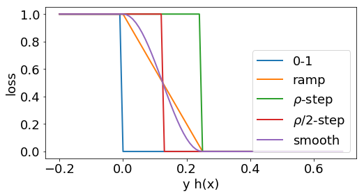
Figure 1: Illustration of different choices of function $\phi$ for $\rho=0.25$.

We now introduce some notation needed for the presentation and discussion of our relative deviation margin bound. Let $\phi\colon\mathbb{R}\to\mathbb{R}_{+}$ be a function such that the following inequality holds for all $x\in\mathbb{R}$:

$$1_{x<0}\leq\phi(x)\leq 1_{x<\rho}.$$

As an example, we can choose $\phi(x)=1_{x<\rho/2}$ as in the previous sections. For a sample $z=(x,y)$, let $g(z)=\phi(yh(x))$. Then,

$$1_{yh(x)<0}\leq g(z)\leq 1_{yh(x)<\rho}.$$ (3)

Let the family ${\mathscr{G}}$ be defined as follows: ${\mathscr{G}}=\{z=(x,y)\mapsto\phi(yh(x))\colon h\in{\mathscr{H}}\}$ and let $R(g)=\operatorname*{\mathbb{E}}_{z\sim{\mathscr{D}}}[g(z)]$ denote the expectation of $g$ and $\widehat{R}_{S}(g)=\operatorname*{\mathbb{E}}_{z\sim S}[g(z)]$ its empirical expectation for a sample $S$. There are several choices for function $\phi$, as illustrated by Figure 1. For example, $\phi(x)$ can be chosen to be $1_{x<\rho}$ or $1_{x<\rho/2}$ (Bartlett, 1998). $\phi$ can also be chosen to be the so-called ramp loss:

$$\phi(x)=\begin{cases}1&\text{if }x<0\\ 1-\frac{x}{\rho}&\text{if }x\in[0,\rho]\\ 0&\text{if }x>\rho,\end{cases}$$

or the smoothed margin loss chosen by (Srebro et al., 2010):

$$\phi(x)=\begin{cases}1&\text{if }x<0\\ \frac{1+\cos(\pi x/\rho)}{2}&\text{if }x\in[0,\rho]\\ 0&\text{if }x>\rho.\end{cases}$$

Fix $\rho>0$. Define the $\rho$-truncation function $\beta_{\rho}\colon\mathbb{R}\to[-\rho,+\rho]$ by $\beta_{\rho}(u)=\max\set{u,-\rho}1_{u\leq 0}+\min\set{u,+\rho}1_{u\geq 0}$, for all $u\in\mathbb{R}$. For any $h\in{\mathscr{H}}$, we denote by $h_{\rho}$ the $\rho$-truncation of $h$, $h_{\rho}=\beta_{\rho}(h)$, and define ${\mathscr{H}}_{\rho}=\set{h_{\rho}\colon h\in{\mathscr{H}}}$.

For any family of functions ${\mathscr{F}}$, we also denote by $\mathcal{N}_{\infty}({\mathscr{F}},\epsilon,x_{1}^{m})$ the empirical covering number of ${\mathscr{F}}$ over the sample $(x_{1},\ldots,x_{m})$ and by ${\mathscr{C}}({\mathscr{F}},\epsilon,x_{1}^{m})$ a minimum empirical cover. Then, the following symmetrization lemma holds.

Lemma 2.2.

Fix $\rho\geq 0$ and $1<\alpha\leq 2$. Then, the following inequality holds:

$$\operatorname*{\mathbb{P}}_{S,S^{\prime}\sim{\mathscr{D}}^{m}}\left[\sup_{h\in{\mathscr{H}}}\frac{\widehat{R}_{S^{\prime}}(h)-\widehat{R}^{\rho}_{S}(h)}{\sqrt[\alpha]{\frac{1}{2}[\widehat{R}_{S^{\prime}}(h)+\widehat{R}^{\rho}_{S}(h)+\frac{1}{m}]}}>\epsilon\right]\leq\operatorname*{\mathbb{P}}_{S,S^{\prime}\sim{\mathscr{D}}^{m}}\left[\sup_{g\in{\mathscr{G}}}\frac{\widehat{R}_{S^{\prime}}(g)-\widehat{R}_{S}(g)}{\sqrt[\alpha]{\frac{1}{2}[\widehat{R}_{S^{\prime}}(g)+\widehat{R}_{S}(g)+\frac{1}{m}]}}>\epsilon\right].$$

Further for $g(z)=1_{yh(x)<\rho/2}$, using the shorthand ${\mathscr{K}}={\mathscr{C}}({\mathscr{H}}_{\rho},\frac{\rho}{2},S\cup S^{\prime})$, the following holds:

$$\operatorname*{\mathbb{P}}_{S,S^{\prime}\sim{\mathscr{D}}^{m}}\left[\sup_{h\in{\mathscr{H}}}\frac{\widehat{R}_{S^{\prime}}(h)-\widehat{R}^{\rho}_{S}(h)}{\sqrt[\alpha]{\frac{1}{2}[\widehat{R}_{S^{\prime}}(h)+\widehat{R}^{\rho}_{S}(h)+\frac{1}{m}]}}>\epsilon\right]\leq\operatorname*{\mathbb{P}}_{S,S^{\prime}\sim{\mathscr{D}}^{m}}\left[\sup_{h\in{\mathscr{K}}}\frac{\widehat{R}^{\frac{\rho}{2}}_{S^{\prime}}(h)-\widehat{R}^{\frac{\rho}{2}}_{S}(h)}{\sqrt[\alpha]{\frac{1}{2}[\widehat{R}^{\frac{\rho}{2}}_{S^{\prime}}(h)+\widehat{R}^{\frac{\rho}{2}}_{S}(h)+\frac{1}{m}]}}>\epsilon\right].$$

The proof consists of using inequality 3, it is given in Appendix A. The first result of the lemma gives an upper bound for a general choice of functions $g$, that is for an arbitrary choices of the $\Phi$ loss function. This inequality will be used in Section 4 to derive our Rademacher complexity bounds. The second inequality is for the specific choice of $\Phi$ that corresponds to $\rho/2$-step function. We will use this inequality in the next section to derive $\ell_{\infty}$ covering number bounds.

3 Relative deviation margin bounds – Covering numbers

In this section, we present a general relative deviation margin-based learning bound, expressed in terms of the expected empirical covering number of ${\mathscr{H}}_{\rho}$. The learning guarantee is thus distribution-dependent. It is also very general since it is given for any $1\!<\!\alpha\!\leq\!2$ and an arbitrary hypothesis set.

Theorem 3.1 (General relative deviation margin bound).

Fix $\rho\geq 0$ and $1<\alpha\leq 2$. Then, for any hypothesis set ${\mathscr{H}}$ of functions mapping from ${\mathscr{X}}$ to $\mathbb{R}$ and any $\tau>0$, the following inequality holds:

$$\operatorname*{\mathbb{P}}_{S\sim{\mathscr{D}}^{m}}\left[\sup_{h\in{\mathscr{H}}}\frac{R(h)-\widehat{R}^{\rho}_{S}(h)}{\sqrt[\alpha]{R(h)+\tau}}>\epsilon\right]\leq 4\,\operatorname*{\mathbb{E}}_{x_{1}^{2m}\sim{\mathscr{D}}^{2m}}[\mathcal{N}_{\infty}({\mathscr{H}}_{\rho},\tfrac{\rho}{2},x_{1}^{2m})]\ \exp\left[\frac{-m^{\frac{2(\alpha-1)}{\alpha}}\epsilon^{2}}{2^{\frac{\alpha+2}{\alpha}}}\right].$$

The proof is given in Appendix B. As mentioned earlier, a version of this result for $\alpha=2$ was postulated by Bartlett (1998). The result can be alternatively expressed as follows, taking the limit $\tau\to 0$.

Corollary 3.2.

Fix $\rho\geq 0$ and $1<\alpha\leq 2$. Then, for any hypothesis set ${\mathscr{H}}$ of functions mapping from ${\mathscr{X}}$ to $\mathbb{R}$, with probability at least $1-\delta$, the following inequality holds for all $h\in{\mathscr{H}}$:

$$R(h)\leq\widehat{R}^{\rho}_{S}(h)+2^{\frac{\alpha+2}{2\alpha}}\sqrt[\alpha]{R(h)}\sqrt{\frac{\log\operatorname*{\mathbb{E}}[\mathcal{N}_{\infty}({\mathscr{H}}_{\rho},\tfrac{\rho}{2},x_{1}^{2m})]+\log\frac{1}{\delta}}{m^{\frac{2(\alpha-1)}{\alpha}}}}.$$

Note that a smaller value of $\alpha$ ($\alpha$ closer to $1$) might be advantageous for some values of $R(h)$, at the price of a worse complexity in terms of the sample size. For $\alpha=2$, the result can be rewritten as follows.

Corollary 3.3.

Fix $\rho\geq 0$. Then, for any hypothesis set ${\mathscr{H}}$ of functions mapping from ${\mathscr{X}}$ to $\mathbb{R}$, with probability at least $1-\delta$, the following inequality holds for all $h\in{\mathscr{H}}$:

$$R(h)\leq\widehat{R}^{\rho}_{S}(h)+2\sqrt{\widehat{R}^{\rho}_{S}(h)\frac{\log\operatorname*{\mathbb{E}}[\mathcal{N}_{\infty}({\mathscr{H}}_{\rho},\tfrac{\rho}{2},x_{1}^{2m})]+\log\frac{1}{\delta}}{m}}+4\frac{\log\operatorname*{\mathbb{E}}[\mathcal{N}_{\infty}({\mathscr{H}}_{\rho},\tfrac{\rho}{2},x_{1}^{2m})]+\log\frac{1}{\delta}}{m}.$$

Proof 3.4.

Let $a=R(h)$, $b=\widehat{R}^{\rho}_{S}(h)$, and $c=\frac{\log\operatorname*{\mathbb{E}}[\mathcal{N}_{\infty}({\mathscr{H}}_{\rho},\tfrac{\rho}{2},x_{1}^{2m})),\frac{\rho}{2})]+\log\frac{1}{\delta}}{m}$. Then, for $\alpha=2$, the inequality of Corollary 3.2 can be rewritten as

$$a\leq b+2\sqrt{ca}.$$

This implies that $(\sqrt{a}-\sqrt{c})^{2}\leq b+c$ and hence $\sqrt{a}\leq\sqrt{b+c}+\sqrt{c}$. Therefore, $a\leq b+2c+2\sqrt{(b+c)c}\leq b+4c+2\sqrt{cb}$. Substituting the values of $a,b,$ and $c$ yields the bound.

The guarantee just presented provides a tighter margin-based learning bound than standard margin bounds since the dominating term admits the empirical margin loss as a factor. Standard margin bounds are subject to a trade-off: a large value of $\rho$ reduces the complexity term while leading to a larger empirical margin loss term. Here, the presence of the empirical loss factor favors this trade-off by allowing a smaller choice of $\rho$. The bound is distribution-dependent since it is expressed in terms of the expected covering number and it holds for an arbitrary hypothesis set ${\mathscr{H}}$.

The learning bounds just presented hold for a fixed value of $\rho$. They can be extended to hold uniformly for all values of $\rho\in[0,1]$, at the price of an additional $\log\log$-term. We illustrate that extension for Corollary 3.2.

Corollary 3.5.

Fix $1<\alpha\leq 2$. Then, for any hypothesis set ${\mathscr{H}}$ of functions mapping from ${\mathscr{X}}$ to $\mathbb{R}$ and any $\rho\in(0,r]$, with probability $\geq 1-\delta$, the following inequality holds for all $h\in{\mathscr{H}}$:

$$R(h)\leq\widehat{R}^{\rho}_{S}(h)+2^{\frac{\alpha+2}{2\alpha}}\sqrt[\alpha]{R(h)}\sqrt{\frac{\log\operatorname*{\mathbb{E}}[\mathcal{N}_{\infty}({\mathscr{H}}_{\rho},\tfrac{\rho}{4},x_{1}^{2m})]+\log\frac{1}{\delta}+\log\log_{2}\frac{2r}{\rho}}{m^{\frac{2(\alpha-1)}{\alpha}}}}.$$

Proof 3.6.

For $k\geq 1$, let $\rho_{k}=r/2^{k}$ and $\delta_{k}=\delta/k^{2}$. For all such $\rho_{k}$, by Corollary 3.2 and the union bound,

$$R(h)\leq\widehat{R}^{\rho_{k}}_{S}(h)+2^{\frac{\alpha+2}{2\alpha}}\sqrt[\alpha]{R(h)}\sqrt{\frac{\log\operatorname*{\mathbb{E}}[\mathcal{N}_{\infty}({\mathscr{H}}_{\rho},\tfrac{\rho_{k}}{2},x_{1}^{2m})]+\log\frac{1}{\delta}+2\log k}{m^{\frac{2(\alpha-1)}{\alpha}}}}.$$

By the union bound, the error probability is most $\sum_{k}\delta_{k}=\delta\sum_{k}(1/k^{2})\leq\delta$. For any $\rho\in(0,r]$, there exists a $k$ such that $\rho\in(\rho_{k},\rho_{k-1}]$. For this $k$, $\rho\leq\rho_{k-1}=r/2^{k-1}$. Hence, $k\leq\log_{2}(2r/\rho)$. By the definition of margin, for all $h\in{\mathscr{H}}$, $\widehat{R}^{\rho_{k}}_{S}(h)\leq\widehat{R}^{\rho}_{S}(h)$. Furthermore, as $\rho_{k}=\rho_{k-1}/2\geq\rho/2$, $\mathcal{N}_{\infty}({\mathscr{H}}_{\rho},\frac{\rho_{k}}{2},x_{1}^{2m})\leq\mathcal{N}_{\infty}({\mathscr{H}}_{\rho},\frac{\rho}{4},x_{1}^{2m})$. Hence, for all $\rho\in(0,r]$,

$$R(h)\leq\widehat{R}^{\rho}_{S}(h)+2^{\frac{\alpha+2}{2\alpha}}\sqrt[\alpha]{R(h)}\sqrt{\frac{\log\operatorname*{\mathbb{E}}[\mathcal{N}_{\infty}({\mathscr{H}}_{\rho},\tfrac{\rho}{4},x_{1}^{2m})]+\log\frac{1}{\delta}+\log\log_{2}\frac{2r}{\rho}}{m^{\frac{2(\alpha-1)}{\alpha}}}}.$$

Our previous bounds can be expressed in terms of the fat-shattering dimension, as illustrated below. Recall that, given $\gamma>0$, a set of points ${\mathscr{U}}=\set{u_{1},\ldots,u_{m}}$ is said to be $\gamma$-shattered by a family of real-valued functions ${\mathscr{H}}$ if there exist real numbers $(r_{1},\ldots,r_{m})$ (witnesses) such that for all binary vectors $(b_{1},\ldots,b_{m})\in\set{0,1}^{m}$, there exists $h\in{\mathscr{H}}$ such that:

$$h(x)\begin{cases}\geq r_{i}+\gamma&\text{if }b_{i}=1;\\ \leq r_{i}-\gamma&\text{otherwise}.\end{cases}$$

The fat-shattering dimension $\operatorname{fat}_{\gamma}({\mathscr{H}})$ of the family ${\mathscr{H}}$ is the cardinality of the largest set $\gamma$-shattered set by ${\mathscr{H}}$ (Anthony and Bartlett, 1999).

Corollary 3.7.

Fix $\rho\geq 0$. Then, for any hypothesis set ${\mathscr{H}}$ of functions mapping from ${\mathscr{X}}$ to $\mathbb{R}$ with $d=\operatorname{fat}_{\frac{\rho}{16}}({\mathscr{H}})$, with probability at least $1-\delta$, the following holds for all $h\in{\mathscr{H}}$:

$$R(h)\leq\widehat{R}^{\rho}_{S}(h)+2\sqrt{\widehat{R}^{\rho}_{S}(h)\frac{1+d\log_{2}(2c^{2}m)\log_{2}\frac{2cem}{d}+\log\frac{1}{\delta}}{m}}+\frac{1+d\log_{2}(2c^{2}m)\log_{2}\frac{2cem}{d}+\log\frac{1}{\delta}}{m},$$

where $c=17$.

Proof 3.8.

By (Bartlett, 1998, Proof of theorem 2), we have

$$\log\max_{x_{1}^{2m}}[\mathcal{N}_{\infty}({\mathscr{H}}_{\rho},\tfrac{\rho}{2},x_{1}^{2m})\leq 1+d^{\prime}\log_{2}(2c^{2}m)\log_{2}\frac{2cem}{d^{\prime}},$$

where $d^{\prime}=\operatorname{fat}_{\frac{\rho}{16}}({\mathscr{H}}_{\rho})\leq\operatorname{fat}_{\frac{\rho}{16}}({\mathscr{H}})=d$. Upper bounding the expectation by the maximum completes the proof.

We will use this bound in Section 6 to derive explicit guarantees for several standard hypothesis sets.

4 Relative deviation margin bounds – Rademacher complexity

In this section, we present relative deviation margin bounds expressed in terms of the Rademacher complexity of the hypothesis sets. As with the previous section, these bounds are general: they hold for any $1<\alpha\leq 2$ and arbitrary hypothesis sets.

As in the previous section, we will define the family ${\mathscr{G}}$ by ${\mathscr{G}}=\set{\phi(yh(x))\colon h\in{\mathscr{H}}}$, where $\phi$ is a function such that

$$1_{x<0}\leq\phi(x)\leq 1_{x<\rho}.$$

4.1 Rademacher complexity-based margin bounds

We first relate the symmetric relative deviation bound to a quantity similar to the Rademacher average, modulo a rescaling.

Lemma 4.1.

Fix $1<\alpha\leq 2$. Then, the following inequality holds:

$$\operatorname*{\mathbb{P}}_{S,S^{\prime}\sim{\mathscr{D}}^{m}}\left[\sup_{g\in{\mathscr{G}}}\frac{\widehat{R}_{S^{\prime}}(g)-\widehat{R}_{S}(g)}{\sqrt[\alpha]{\frac{1}{2}[\widehat{R}_{S^{\prime}}(g)+\widehat{R}_{S}(g)+\frac{1}{m}]}}>\epsilon\right]\leq 2\operatorname*{\mathbb{P}}_{z_{1}^{m}\sim{\mathscr{D}}^{m},{\boldsymbol{\sigma}}}\left[\sup_{g\in{\mathscr{G}}}\frac{\frac{1}{m}\sum_{i=1}^{m}\sigma_{i}g(z_{i})}{\sqrt[\alpha]{\frac{1}{m}[\sum_{i=1}^{m}(g(z_{i}))+1]}}>\frac{\epsilon}{2\sqrt{2}}\right].$$

The proof is given in Appendix C. It consists of introducing Rademacher variables and deriving an upper bound in terms of the first $m$ points only.

Now, to bound the right-hand side of the Lemma 4.1, we use a peeling argument, that is we partition ${\mathscr{G}}$ into subsets ${\mathscr{G}}_{k}$, give a learning bound for each ${\mathscr{G}}_{k}$, and then take a weighted union bound. For any non-negative integer $k$ with $0\leq k\leq\log_{2}m$, let ${\mathscr{G}}_{k}(z_{1}^{m})$ denote the family of hypotheses defined by

$${\mathscr{G}}_{k}(z_{1}^{m})=\set[\bigg{]}{g\in{\mathscr{G}}\colon 2^{k}\leq\Big{(}\sum_{i=1}^{m}g(z_{i})\Big{)}+1<2^{k+1}}.$$

Using the above inequality and a peeling argument, we show the following upper bound expressed in terms of Rademacher complexities.

Lemma 4.2.

Fix $1<\alpha\leq 2$ and $z_{1}^{m}\in{\mathscr{Z}}^{m}$. Then, the following inequality holds:

$$\operatorname*{\mathbb{P}}_{{\boldsymbol{\sigma}}}\left[\sup_{g\in{\mathscr{G}}}\frac{\frac{1}{m}\sum_{i=1}^{m}\sigma_{i}g(z_{i})}{\sqrt[\alpha]{\frac{1}{m}[\sum_{i=1}^{m}(g(z_{i}))+1]}}>{\epsilon}\,\Bigg{\mid}\,z^{m}\right]\leq 2\sum_{k=0}^{\lfloor\log_{2}m\rfloor}\exp\left(\frac{m^{2}\widehat{\mathfrak{R}}_{m}^{2}({\mathscr{G}}_{k}(z_{1}^{m}))}{2^{k+5}}-\frac{\epsilon^{2}}{64\frac{2^{k(1-2/\alpha)}}{m^{2-2/\alpha}}}\right)1_{\epsilon\leq 2\left(\frac{2^{k}}{m}\right)^{1-1/\alpha}}.$$

The proof is given in Appendix C. Instead of applying Hoeffding’s bound to each term of the left-hand side for a fixed $g$ and then using covering and the union bound to bound the supremum, here, we seek to bound the supremum over ${\mathscr{G}}$ directly. To do so, we use a bounded difference inequality that leads to a finer result than McDiarmid’s inequality.

Let $\mathfrak{r}_{m}({\mathscr{G}})$ be defined as the following peeling-based Rademacher complexity of ${\mathscr{G}}$:

$$\mathfrak{r}_{m}({\mathscr{G}})=\sup_{0\leq k\leq\log_{2}(m)}\log\left[\operatorname*{\mathbb{E}}_{z_{1}^{m}\sim{\mathscr{D}}^{m}}\left[\exp\left(\frac{m^{2}\widehat{\mathfrak{R}}_{m}^{2}({\mathscr{G}}_{k}(z_{1}^{m}))}{2^{k+5}}\right)\right]\,\right].$$

Then, the following is a margin-based relative deviation bound expressed in terms of $\mathfrak{r}_{m}({\mathscr{G}})$, that is in terms of Rademacher complexities.

Theorem 4.3.

Fix $1<\alpha\leq 2$. Then, with probability at least $1-\delta$, for all hypothesis $h\in{\mathscr{H}}$, the following inequality holds:

$$R(h)-\widehat{R}^{\rho}_{S}(h) \leq 16\sqrt{2}\sqrt[\alpha]{R(h)}\left(\frac{\mathfrak{r}_{m}({\mathscr{G}})+\log\log m+\log\frac{16}{\delta}}{m}\right)^{1-1/\alpha}$$

$$=16\sqrt{2}\left(\frac{\mathfrak{r}_{m}({\mathscr{G}})+\log\log m+\log\frac{16}{\delta}}{m}\right)\left(\frac{mR(h)}{\mathfrak{r}_{m}({\mathscr{G}})+\log\log m+\log\frac{16}{\delta}}\right)^{1/\alpha}.$$

Combining the above lemma with Theorem 4.3 yields the following.

Corollary 4.4.

Fix $1<\alpha\leq 2$ and let ${\mathscr{G}}$ be defined as above. Then, with probability at least $1-\delta$, for all hypothesis $h\in{\mathscr{H}}$,

$$R(h)-\widehat{R}^{\rho}_{S}(h)\leq 32\sqrt[\alpha]{\widehat{R}^{\rho}_{S}(h)}\left(\frac{\mathfrak{r}_{m}({\mathscr{G}})+\log\log m+\log\frac{16}{\delta}}{m}\right)^{1-\frac{1}{\alpha}}\mspace{-10.0mu}+\ 2(32)^{\frac{\alpha}{\alpha-1}}\left(\frac{\mathfrak{r}_{m}({\mathscr{G}})+\log\log m+\log\frac{16}{\delta}}{m}\right).$$

The above result can be extended to hold for all $\alpha$ simultaneously.

Corollary 4.5.

Let ${\mathscr{G}}$ be defined as above. Then, with probability at least $1-\delta$, for all hypothesis $h\in{\mathscr{H}}$ and $\alpha\in(1,2]$,

$$R(h)-\widehat{R}^{\rho}_{S}(h)\leq 32\sqrt{2}\sqrt[\alpha]{R(h)}\left(\frac{\mathfrak{r}_{m}({\mathscr{G}})+\log\log m+\log\frac{16}{\delta}}{m}\right)^{1-1/\alpha}.$$

4.2 Upper bounds on peeling-based Rademacher complexity

We now present several upper bounds on $\mathfrak{r}_{m}({\mathscr{G}})$. We provide proofs for all the results in Appendix D. For any hypothesis set ${\mathscr{G}}$, we denote by $\mathbb{S}_{{\mathscr{G}}}({x_{1}^{m}})$ the number of distinct dichotomies generated by ${\mathscr{G}}$ over that sample:

$$\mathbb{S}_{{\mathscr{G}}}({z_{1}^{m}})=\operatorname{Card}\left(\set[\Big{]}{\big{(}g(z_{1}),\ldots,g(z_{m})\big{)}\colon g\in{\mathscr{G}}}\right).$$

We note that we do not make any assumptions over range of ${\mathscr{G}}$.

Lemma 4.6.

If the range of $g$ is in $\{0,1\}$, then the following upper bounds hold on the peeling-based Rademacher complexity of ${\mathscr{G}}$:

$$\mathfrak{r}_{m}({\mathscr{G}})\leq\frac{1}{8}\log\operatorname*{\mathbb{E}}_{z_{1}^{m}}[\mathbb{S}_{{\mathscr{G}}}({z_{1}^{m}})].$$

Combining the above result with Corollary 4.4, improves the relative deviation bounds of (Cortes et al., 2019, Corollary 2) for $\alpha<2$. In particular, we improve the $\sqrt{\operatorname*{\mathbb{E}}_{z_{1}^{m}}[\mathbb{S}_{{\mathscr{G}}}({z_{1}^{m}})]}$ term in their bounds to $\left(\operatorname*{\mathbb{E}}_{z_{1}^{m}}[\mathbb{S}_{{\mathscr{G}}}({z_{1}^{m}})]\right)^{1-1/\alpha}$, which is an improvement for $\alpha<2$.

We next upper bound the peeling based Rademacher complexity in terms of the covering number.

Lemma 4.7.

For a set of hypotheses ${\mathscr{G}}$,

$$\mathfrak{r}_{m}({\mathscr{G}})\leq\sup_{0\leq k\leq\log_{2}(m)}\log\left[\operatorname*{\mathbb{E}}_{z_{1}^{m}\sim{\mathscr{D}}^{m}}\left[\exp\left\{\frac{1}{16}\left(1+\int^{1}_{\frac{1}{\sqrt{m}}}\log N_{2}\left({\mathscr{G}}_{k}(z_{1}^{m}),\sqrt{\tfrac{2^{k}}{m}}\,\epsilon,z_{1}^{m}\right)\,d\epsilon\right)\right\}\right]\,\right].$$

One can further simplify the above bound using the smoothed margin loss from Srebro et al. (2010). Let the worst case Rademacher complexity be defined as follows.

$$\widehat{\mathfrak{R}}_{m}^{\max}({\mathscr{H}})=\sup_{z^{m}_{1}}\widehat{\mathfrak{R}}_{m}({\mathscr{H}}).$$

Lemma 4.8.

Let $g$ be the smoothed margin loss from (Srebro et al., 2010, Section 5.1), with its second moment bounded by $\pi^{2}/4\rho^{2}$. Then, the following holds:

$$\mathfrak{r}_{m}({\mathscr{G}})\leq\frac{16\pi^{2}m}{\rho^{2}}(\widehat{\mathfrak{R}}^{\max}_{m})^{2}({\mathscr{H}})\left(2\log^{3/2}\frac{m}{\widehat{\mathfrak{R}}_{m}^{\max}({\mathscr{H}})}-\log^{3/2}\frac{2\pi m}{\rho\widehat{\mathfrak{R}}_{m}^{\max}({\mathscr{H}})}\right)^{2}.$$

Combining Lemma 4.8 with Corollary 4.4 yields the following bound, which is a generalization of (Srebro et al., 2010, Theorem 5) holding for all $\alpha\in(1,2]$. Furthermore, our constants are more favorable.

Corollary 4.9.

For any $\delta>0$, with probability at least $1-\delta$, the following inequality holds for all $\alpha\in(0,1]$ and all $h\in{\mathscr{H}}$:

$$R(h)-\widehat{R}^{\rho}_{S}(h)\leq 32\sqrt{2}\sqrt[\alpha]{\widehat{R}^{\rho}_{S}(h)}\,\beta_{m}^{1-\frac{1}{\alpha}}+\ 2(32)^{\frac{\alpha}{\alpha-1}}\beta_{m},$$

where

$$\beta_{m}=\frac{16\pi^{2}}{\rho^{2}}(\widehat{\mathfrak{R}}^{\max}_{m})^{2}({\mathscr{H}})\left[2\log^{3/2}\frac{m}{\widehat{\mathfrak{R}}_{m}^{\max}({\mathscr{H}})}-\log^{3/2}\frac{2\pi m}{\rho\widehat{\mathfrak{R}}_{m}^{\max}({\mathscr{H}})}\right]^{2}+\frac{\log\log m+\log\frac{16}{\delta}}{m}.$$

5 Generalization bounds for unbounded loss functions

Standard generalization bounds hold for bounded loss functions. For the more general and more realistic case of unbounded loss functions, a number of different results have been presented in the past, under different assumption on the family of functions. This includes learning bounds assuming the existence of an envelope, that is a single non-negative function with a finite expectation lying above the absolute value of the loss of every function in the hypothesis set (Dudley, 1984; Pollard, 1984; Dudley, 1987; Pollard, 1989; Haussler, 1992), or an assumption similar to Hoeffding’s inequality based on the expectation of a hyperbolic function, a quantity similar to the moment-generating function (Meir and Zhang, 2003), or the weaker assumption that the $\alpha$th-moment of the loss is bounded for some value of $\alpha>1$ (Vapnik, 1998b, 2006b; Cortes et al., 2019). Here, we will also adopt this latter assumption and present distribution-dependent learning bounds for unbounded losses that improve upon the previous bounds of Cortes et al. (2019). To do so, we will leverage the relative deviation margin bounds given in the previous sections, which hold for any $\alpha\leq 2$.

Let $L$ be an unbounded loss function and $L(h,z)$ denote the loss of hypothesis $h$ for sample $z$. Let ${\mathscr{L}}_{\alpha}(h)=\operatorname*{\mathbb{E}}_{z\sim D}[L(h,z)^{\alpha}]$ be the $\alpha^{\text{th}}$-moment of the loss function ${\mathscr{L}}$, which is assumed finite for all $h\in{\mathscr{H}}$. In what follows, we will use the shorthand $\operatorname*{\mathbb{P}}[L(h,z)>t]$ instead of $\operatorname*{\mathbb{P}}_{z\sim D}[L(h,z)>t]$, and similarly $\widehat{\operatorname*{\mathbb{P}}}[L(h,z)>t]$ instead of $\operatorname*{\mathbb{P}}_{z\sim\widehat{D}}[L(h,z)>t]$.

Theorem 5.1.

Fix $\rho\geq 0$. Let $1<\alpha\leq 2$, $0<\epsilon\leq 1$, and $0<\tau^{\frac{\alpha-1}{\alpha}}<\epsilon^{\frac{\alpha}{\alpha-1}}$. For any loss function $L$ (not necessarily bounded) and hypothesis set ${\mathscr{H}}$ such that ${\mathscr{L}}_{\alpha}(h)<+\infty$ for all $h\in{\mathscr{H}}$,

$$\operatorname*{\mathbb{P}}\left[\sup_{h\in H}{\mathscr{L}}(h)-\widehat{\mathscr{L}}_{S}(h)\,>{\Gamma}_{\tau}(\alpha,\epsilon)\,\epsilon{\sqrt[\alpha]{{\mathscr{L}}_{\alpha}(h)+\tau}}+\rho\right]\\ \leq\operatorname*{\mathbb{P}}\left[\sup_{h\in{\mathscr{H}},t\in\mathbb{R}}\frac{\operatorname*{\mathbb{P}}[L(h,z)>t]-\widehat{\operatorname*{\mathbb{P}}}[L(h,z)>t-\rho]}{{\sqrt[\alpha]{\operatorname*{\mathbb{P}}[L(h,z)>t]+\tau}}}>\epsilon\right],$$

where ${\Gamma}_{\tau}(\alpha,\epsilon)=\frac{\alpha-1}{\alpha}(1+\tau)^{\frac{1}{\alpha}}+\frac{1}{\alpha}\left(\frac{\alpha}{\alpha-1}\right)^{\alpha-1}(1+\left(\frac{\alpha-1}{\alpha}\right)^{\alpha}\tau^{\frac{1}{\alpha}})^{\frac{1}{\alpha}}\left[1+\frac{\log(1/\epsilon)}{\left(\frac{\alpha}{\alpha-1}\right)^{\alpha-1}}\right]^{\frac{\alpha-1}{\alpha}}$ .

The proof is provided in Appendix E. The above theorem can be used in conjunction with our relative deviation margin bounds to obtain strong guarantees for unbounded loss functions and we illustrate it with our $\ell_{\infty}$ based bounds. Similar techniques can be used to obtain peeling-based Rademacher complexity bounds. Combining Theorems 5.1 and (3.1) yields the following corollary.

Corollary 5.2.

Fix $\rho\geq 0$. Let $\epsilon<1$, $1<\alpha\leq 2$. and hypothesis set ${\mathscr{H}}$ such that ${\mathscr{L}}_{\alpha}(h)<+\infty$ for all $h\in{\mathscr{H}}$,

$${\mathscr{L}}(h)-\widehat{\mathscr{L}}_{S}(h) \leq\gamma\sqrt[\alpha]{{\mathscr{L}}_{\alpha}(h)}\sqrt{\frac{\log\operatorname*{\mathbb{E}}[\mathcal{N}_{\infty}({\mathscr{L}}({\mathscr{H}}),\tfrac{\rho}{2},x_{1}^{2m})]+\log\frac{1}{\delta}}{m^{\frac{2(\alpha-1)}{\alpha}}}}+\rho,$$

where $\gamma=\Gamma_{0}\left(\alpha,\sqrt{\frac{\log\operatorname*{\mathbb{E}}[\mathcal{N}_{\infty}({\mathscr{L}}({\mathscr{H}}),\tfrac{\rho}{2},x_{1}^{2m})]+\log\frac{1}{\delta}}{m^{\frac{2(\alpha-1)}{\alpha}}}}\right)=\mathcal{O}(\log m)$.

The upper bound in the above corollary has two terms. The first term is based on the covering number and decreases with $\rho$ while the second term increases with $\rho$. One can choose a suitable value of $\rho$ that minimizes the sum to obtain favorable bounds. Furthermore, the above bound depends on the covering number as opposed to the result of Cortes et al. (2019), which depends on the number of dichotomies generated by the hypothesis set. Hence, the above bound is optimistic and in general is more favorable than the previous known bounds of Cortes et al. (2019). We note that instead of using the $\ell_{\infty}$ based bounds, one can use the Rademacher complexity bounds to obtain better results.

6 Applications

In this section, we briefly highlight some applications of our learning bounds: both our covering number and Rademacher complexity margin bounds can be used to derive finer margin-based guarantees for several commonly used hypothesis sets. Below we briefly illustrate these applications.

Linear hypothesis sets: let ${\mathscr{H}}$ be the family of liner hypotheses defined by

$${\mathscr{H}}=\set{{\mathbf{x}}\mapsto{\mathbf{w}}\cdot{\mathbf{x}}\colon\|{\mathbf{w}}\|_{2}\leq 1,{\mathbf{x}}\in\mathbb{R}^{n},\|{\mathbf{x}}\|_{2}\leq R}.$$

Then, the following upper bound holds for the fat-shattering dimension of ${\mathscr{H}}$ (Bartlett and Shawe-Taylor, 1998): $\operatorname{fat}_{\rho}({\mathscr{H}})\leq(R/\rho)^{2}$. Plugging in this upper bound in the bound of Corollary 3.7 yields the following:

$$R(h)\leq\widehat{R}^{\rho}_{S}(h)+2\sqrt{\widehat{R}^{\rho}_{S}(h)\,\beta_{m}}+\beta_{m},$$ (4)

with $\beta_{m}=\widetilde{O}\left(\frac{(R/\rho)^{2}}{m}\right)$. In comparison, the best existing margin bound for SVM by (Bartlett and Shawe-Taylor, 1998, Theorem 1.7) is

$$R(h)\leq\widehat{R}^{\rho}_{S}(h)+c^{\prime}\sqrt{\beta^{\prime}_{m}},$$ (5)

where $c^{\prime}$ is some universal constant and where $\beta^{\prime}_{m}=\widetilde{O}\left(\frac{(R/\rho)^{2}}{m}\right)$. The margin bound (4) is thus more favorable than (5).

Ensembles of predictors in base hypothesis set ${\mathscr{H}}$: let $d$ be the VC-dimension of ${\mathscr{H}}$ and consider the family of ensembles ${\mathscr{F}}=\set{x\mapsto\sum_{k=1}^{p}w_{k}h_{k}(x)\colon h_{k}\in{\mathscr{H}},w_{k}\geq 0,\sum_{k=1}^{p}w_{k}=1}$. Then, the following upper bound on the fat-shattering dimension holds (Bartlett and Shawe-Taylor, 1998): $\operatorname{fat}_{\rho}({\mathscr{F}})\leq c(d/\rho)^{2}\log(1/\rho)$, for some universal constant $c$. Plugging in this upper bound in the bound of Corollary 3.7 yields the following:

$$R(h)\leq\widehat{R}^{\rho}_{S}(h)+2\sqrt{\widehat{R}^{\rho}_{S}(h)\,\beta_{m}}+\beta_{m},$$ (6)

with $\beta_{m}=\widetilde{O}\left(\frac{(d/\rho)^{2}}{m}\right)$. In comparison, the best existing margin bound for ensembles such as AdaBoost in terms of the VC-dimension of the base hypothesis given by Schapire et al. (1997) is:

$$R(h)\leq\widehat{R}^{\rho}_{S}(h)+c^{\prime}\sqrt{\beta^{\prime}_{m}},$$ (7)

where $c^{\prime}$ is some universal constant and where $\beta^{\prime}_{m}=\widetilde{O}\left(\frac{(d/\rho)^{2}}{m}\right)$. The margin bound in (6) is thus more favorable than (7).

Feed-forward neural networks of depth $d$: let ${\mathscr{H}}_{0}=\set{{\mathbf{x}}\mapsto{\mathbf{x}}_{i}\colon i\in\{0,1,\ldots n\},{\mathbf{x}}\in[-1,1]^{n}}\cup\set{0,1}$ and

$${\mathscr{H}}_{i}=\set{\sigma\left(\sum_{h\in\cup_{j<i}{\mathscr{H}}_{j}}{\mathbf{w}}\cdot h\right):\|{\mathbf{w}}\|_{1}\leq R}$$

for $i\in[d]$, where $\sigma$ is a $\mu$-Lipschitz activation function. Then, the following upper bound holds for the fat-shattering dimension of ${\mathscr{H}}$ (Bartlett and Shawe-Taylor, 1998): $\operatorname{fat}_{\rho}({\mathscr{H}}_{d})\leq\frac{c^{d^{2}}(R\mu)^{d(d+1)}}{\rho^{2d}}\log n$. Plugging in this upper bound in the bound of Corollary 3.7 gives the following:

$$R(h)\leq\widehat{R}^{\rho}_{S}(h)+2\sqrt{\widehat{R}^{\rho}_{S}(h)\,\beta_{m}}+\beta_{m},$$ (8)

with $\beta_{m}=\widetilde{O}\left(\frac{c^{d^{2}}(R\mu)^{d(d+1)}/\rho^{2d}}{m}\right)$. In comparison, the best existing margin bound for neural networks by (Bartlett and Shawe-Taylor, 1998, Theorem 1.5 , Theorem 1.11) is

$$R(h)\leq\widehat{R}^{\rho}_{S}(h)+c^{\prime}\sqrt{\beta^{\prime}_{m}},$$ (9)

where $c^{\prime}$ is some universal constant and where $\beta^{\prime}_{m}=\widetilde{O}\left(\frac{c^{d^{2}}(R\mu)^{d(d+1)}/\rho^{2d}}{m}\right)$. The margin bound in (8) is thus more favorable than (9). The Rademacher complexity bounds of Corollary 4.9 can also be used to provide generalization bounds for neural networks. For a matrix ${\mathbf{W}}$, let $\|{\mathbf{W}}\|_{p,q}$ denote the matrix $p,q$ norm and $\|{\mathbf{W}}\|_{2}$ denote the spectral norm. Let ${\mathscr{H}}_{0}=\{{\mathbf{x}}:\|{\mathbf{x}}\|_{2}\leq 1,{\mathbf{x}}\in{\mathbf{R}}^{n}\}$ and ${\mathscr{H}}_{i}=\{\sigma({\mathbf{W}}\cdot h):h\in{\mathscr{H}}_{i-1},\|{\mathbf{W}}\|_{2}\leq R,\|{\mathbf{W}}^{T}\|_{2,1}\leq R_{2,1}\|{\mathbf{W}}\|_{2})\}$. Then, by (Bartlett et al., 2017), the following upper bound holds:

$$\widehat{\mathfrak{R}}_{m}^{\max}({\mathscr{H}})\leq\widetilde{O}\left(\frac{d^{3/2}RR_{2,1}}{\rho^{d}\sqrt{m}}\cdot(RL)^{d}\right).$$

Plugging in this upper bound in the bound of Corollary 4.9 leads to the following:

$$R(h)\leq\widehat{R}^{\rho}_{S}(h)+2\sqrt{\widehat{R}^{\rho}_{S}(h)\,\beta_{m}}+\beta_{m},$$ (10)

where $\beta_{m}=\widetilde{O}\left(\frac{d^{3}R^{2}R^{2}_{2,1}}{\rho^{2d}m}\cdot(RL)^{2d}\right)$. In comparison, the best existing neural network bounds by Bartlett et al. (2017, Theorem 1.1) is

$$R(h)\leq\widehat{R}^{\rho}_{S}(h)+c^{\prime}\sqrt{\beta^{\prime}_{m}},$$ (11)

where $c^{\prime}$ is a universal constant and $\beta^{\prime}_{m}$ is the empirical Rademacher complexity. The margin bound (10) has the benefit of a more favorable dependency on the empirical margin loss than (11), which can be significant when that empirical term is small. On other hand, the empirical Rademacher complexity of (11) is more favorable than its counterpart in (10).

In Appendix F, we further discuss other potential applications of our learning guarantees.

7 Conclusion

We presented a series of general relative deviation margin bounds. These are tighter margin bounds that can serve as useful tools to derive guarantees for a variety of hypothesis sets and in a variety of applications. In particular, these bounds could help derive better margin-based learning bounds for different families of neural networks, which has been the topic of several recent research publications.

Appendix A Symmetrization

We use the following lemmas from Cortes et al. (2019) in our proofs.

Lemma A.1 (Cortes et al. (2019)).

Fix $\eta>0$ and $\alpha$ with $1<\alpha\leq 2$. Let $f\colon(0,+\infty)\times(0,+\infty)\to\mathbb{R}$ be the function defined by $f\colon(x,y)\mapsto\frac{x-y}{\sqrt[\alpha]{x+y+\eta}}$. Then, $f$ is a strictly increasing function of $x$ and a strictly decreasing function of $y$.

Lemma A.2 (Greenberg and Mohri (2013)).

Let $X$ be a random variable distributed according to the binomial distribution $B(m,p)$ with $m$ a positive integer (the number of trials) and $p>\frac{1}{m}$ (the probability of success of each trial). Then, the following inequality holds:

$$\operatorname*{\mathbb{P}}\left[X\geq\operatorname*{\mathbb{E}}[X]\right]>\frac{1}{4},$$ (12)

and, if instead of requiring $p>\frac{1}{m}$ we require $p<1-\frac{1}{m}$, then

$$\operatorname*{\mathbb{P}}\left[X\leq\operatorname*{\mathbb{E}}[X]\right]>\frac{1}{4},$$ (13)

where in both cases $\operatorname*{\mathbb{E}}[X]=mp$.

The following symmetrization lemma in terms of empirical margin loss is proven using the previous lemmas.

Lemma 2.1

Fix $\rho\geq 0$ and $1<\alpha\leq 2$ and assume that $m\epsilon^{\frac{\alpha}{\alpha-1}}>1$. Then, for any any $\epsilon,\tau>0$, the following inequality holds:

$$\operatorname*{\mathbb{P}}_{S\sim{\mathscr{D}}^{m}}\left[\sup_{h\in{\mathscr{H}}}\frac{R(h)-\widehat{R}^{\rho}_{S}(h)}{\sqrt[\alpha]{R(h)+\tau}}>\epsilon\right]\leq 4\operatorname*{\mathbb{P}}_{S,S^{\prime}\sim{\mathscr{D}}^{m}}\left[\sup_{h\in{\mathscr{H}}}\frac{\widehat{R}_{S^{\prime}}(h)-\widehat{R}^{\rho}_{S}(h)}{\sqrt[\alpha]{\frac{1}{2}[\widehat{R}_{S^{\prime}}(h)+\widehat{R}^{\rho}_{S}(h)+\frac{1}{m}]}}>\epsilon\right].$$

Proof A.3.

We will use the function $F$ defined over $(0,+\infty)\times(0,+\infty)$ by $F\colon(x,y)\mapsto\frac{x-y}{\sqrt[\alpha]{\frac{1}{2}[x+y+\frac{1}{m}]}}$.

Fix $S,S^{\prime}\in{\mathscr{Z}}^{m}$. We first show that the following implication holds for any $h\in{\mathscr{H}}$:

$$\left(\frac{R(h)-\widehat{R}^{\rho}_{S}(h)}{\sqrt[\alpha]{R(h)+\tau}}>\epsilon\right)\wedge\left(\widehat{R}_{S^{\prime}}(h)>R(h)\right)\Rightarrow F(\widehat{R}_{S^{\prime}}(h),\widehat{R}^{\rho}_{S}(h))>\epsilon.$$ (14)

The first condition can be equivalently rewritten as $\widehat{R}^{\rho}_{S}(h)<R(h)-\epsilon\sqrt[\alpha]{(R(h)+\tau)}$, which implies

$$\widehat{R}^{\rho}_{S}(h)<R(h)-\epsilon\sqrt[\alpha]{R(h)}\\ \qquad\wedge\qquad\epsilon^{\frac{\alpha}{\alpha-1}}<R(h),$$ (15)

since $\widehat{R}^{\rho}_{S}(h)\geq 0$. Assume that the antecedent of the implication (14) holds for $h\in{\mathscr{H}}$. Then, in view of the monotonicity properties of function $F$ (Lemma A.1), we can write:

$$F(\widehat{R}_{S^{\prime}}(h),\widehat{R}^{\rho}_{S}(h)) \geq F(R(h),R(h)-\epsilon\sqrt[\alpha]{R(h)}) \widehat{R}_{S^{\prime}}(h)>R(h)$$ ( and 1st ineq. of (15))

$$=\frac{R(h)-(R(h)-\epsilon R(h)^{\frac{1}{\alpha}}}{\sqrt[\alpha]{\frac{1}{2}[2R(h)-\epsilon R(h)^{\frac{1}{\alpha}}+\frac{1}{m}]}}$$

$$\geq\frac{\epsilon R(h)^{\frac{1}{\alpha}}}{\sqrt{\frac{1}{2}[2R(h)-\epsilon^{\frac{\alpha}{\alpha-1}}+\frac{1}{m}]}}$$ (second ineq. of (15))

$$>\frac{\epsilon R(h)^{\frac{1}{\alpha}}}{\sqrt[\alpha]{\frac{1}{2}[2R(h)]}}=\epsilon, m\epsilon^{\frac{\alpha}{\alpha-1}}>1$$ ()

which proves (14).

Now, by definition of the supremum, for any $\eta>0$, there exists $h_{S}\in{\mathscr{H}}$ such that

$$\sup_{h\in{\mathscr{H}}}\frac{R(h)-\widehat{R}^{\rho}_{S}(h)}{\sqrt[\alpha]{R(h)+\tau}}-\frac{R(h_{S})-\widehat{R}^{\rho}_{S}(h_{S})}{\sqrt[\alpha]{R(h_{S})+\tau}}\leq\eta.$$ (16)

Using the definition of $h_{S}$ and the implication (14), we can write

$$\operatorname*{\mathbb{P}}_{S,S^{\prime}\sim{\mathscr{D}}^{m}}\left[\sup_{h\in{\mathscr{H}}}\frac{\widehat{R}_{S^{\prime}}(h)-\widehat{R}^{\rho}_{S}(h)}{\sqrt[\alpha]{\frac{1}{2}[\widehat{R}^{\rho}_{S}(h)+\widehat{R}_{S^{\prime}}(h)+\frac{1}{m}]}}>\epsilon\right]$$

$$\geq\operatorname*{\mathbb{P}}_{S,S^{\prime}\sim{\mathscr{D}}^{m}}\left[\frac{\widehat{R}_{S^{\prime}}(h_{S})-\widehat{R}^{\rho}_{S}(h_{S})}{\sqrt[\alpha]{\frac{1}{2}[\widehat{R}^{\rho}_{S}(h_{S})+\widehat{R}_{S^{\prime}}(h_{S})+\frac{1}{m}]}}>\epsilon\right] \sup$$ (def. of )

$$\geq\operatorname*{\mathbb{P}}_{S,S^{\prime}\sim{\mathscr{D}}^{m}}\left[\left(\frac{R(h_{S})-\widehat{R}^{\rho}_{S}(h_{S})}{\sqrt[\alpha]{R(h_{S})+\tau}}>\epsilon\right)\wedge\left(\widehat{R}_{S^{\prime}}(h_{S})>R(h_{S})\right)\right] (\text{implication (\ref{eq:implication})})$$

$$=\operatorname*{\mathbb{E}}_{S,S^{\prime}\sim{\mathscr{D}}^{m}}\left[1_{\frac{R(h_{S})-\widehat{R}^{\rho}_{S}(h_{S})}{\sqrt[\alpha]{R(h_{S})+\tau}}>\epsilon}1_{\widehat{R}_{S^{\prime}}(h_{S})>R(h_{S})}\right] (\text{def. of expectation})$$

$$=\operatorname*{\mathbb{E}}_{S\sim{\mathscr{D}}^{m}}\left[1_{\frac{R(h_{S})-\widehat{R}^{\rho}_{S}(h_{S})}{\sqrt[\alpha]{R(h_{S})+\tau}}>\epsilon}\operatorname*{\mathbb{P}}_{S^{\prime}\sim{\mathscr{D}}^{m}}\left[\widehat{R}_{S^{\prime}}(h_{S})>R(h_{S})\right]\right].$$ (linearity of expectation)

Now, observe that, if $R(h_{S})\leq\epsilon^{\frac{\alpha}{\alpha-1}}$, then the following inequalities hold:

$$\frac{R(h_{S})-\widehat{R}^{\rho}_{S}(h_{S})}{\sqrt[\alpha]{R(h_{S})+\tau}}\leq\frac{R(h_{S})}{\sqrt[\alpha]{R(h_{S})}}=R(h_{S})^{\frac{\alpha-1}{\alpha}}\leq\epsilon.$$ (17)

In light of that, we can write

$$\operatorname*{\mathbb{P}}_{S,S^{\prime}\sim{\mathscr{D}}^{m}}\left[\sup_{h\in{\mathscr{H}}}\frac{\widehat{R}_{S^{\prime}}(h)-\widehat{R}^{\rho}_{S}(h)}{\sqrt[\alpha]{\frac{1}{2}[\widehat{R}^{\rho}_{S}(h)+\widehat{R}_{S^{\prime}}(h)+\frac{1}{m}]}}>\epsilon\right]$$

$$\geq\operatorname*{\mathbb{E}}_{S\sim{\mathscr{D}}^{m}}\left[1_{\frac{R(h_{S})-\widehat{R}^{\rho}_{S}(h_{S})}{\sqrt[\alpha]{R(h_{S})+\tau}}>\epsilon}1_{R(h_{S})>\epsilon^{\frac{\alpha}{\alpha-1}}}\operatorname*{\mathbb{P}}_{S^{\prime}\sim{\mathscr{D}}^{m}}\left[\widehat{R}_{S^{\prime}}(h_{S})>R(h_{S})\right]\right]$$

$$\geq\frac{1}{4}\operatorname*{\mathbb{E}}_{S\sim{\mathscr{D}}^{m}}\left[1_{\frac{R(h_{S})-\widehat{R}^{\rho}_{S}(h_{S})}{\sqrt[\alpha]{R(h_{S})+\tau}}>\epsilon}\right] (\text{$\epsilon^{\frac{\alpha}{\alpha-1}}>\tfrac{1}{m}$ and Lemma~{}\ref{lem:binomial}})$$

$$\geq\frac{1}{4}\operatorname*{\mathbb{E}}_{S\sim{\mathscr{D}}^{m}}\left[1_{\sup_{h\in{\mathscr{H}}}\frac{R(h)-\widehat{R}^{\rho}_{S}(h)}{\sqrt[\alpha]{R(h)+\tau}}>\epsilon+\eta}\right] (\text{def. of $h_{S}$})$$

$$=\frac{1}{4}\operatorname*{\mathbb{P}}_{S\sim{\mathscr{D}}^{m}}\left[\sup_{h\in{\mathscr{H}}}\frac{R(h)-\widehat{R}^{\rho}_{S}(h)}{\sqrt[\alpha]{R(h)+\tau}}>\epsilon+\eta\right]. (\text{def. of expectation})$$

Now, since this inequality holds for all $\eta>0$, we can take the limit $\eta\to 0$ and use the right-continuity of the cumulative distribution to obtain

$$\operatorname*{\mathbb{P}}_{S,S^{\prime}\sim{\mathscr{D}}^{m}}\left[\sup_{h\in{\mathscr{H}}}\frac{\widehat{R}_{S^{\prime}}(h)-\widehat{R}^{\rho}_{S}(h)}{\sqrt[\alpha]{\frac{1}{2}[\widehat{R}^{\rho}_{S}(h)+\widehat{R}_{S^{\prime}}(h)+\frac{1}{m}]}}>\epsilon\right]\geq\frac{1}{4}\operatorname*{\mathbb{P}}_{S\sim{\mathscr{D}}^{m}}\left[\sup_{h\in{\mathscr{H}}}\frac{R(h)-\widehat{R}^{\rho}_{S}(h)}{\sqrt[\alpha]{R(h)+\tau}}>\epsilon\right],$$

which completes the proof.

Lemma 2.2

Fix $\rho\geq 0$ and $1<\alpha\leq 2$. Then, the following inequality holds:

$$\operatorname*{\mathbb{P}}_{S,S^{\prime}\sim{\mathscr{D}}^{m}}\left[\sup_{h\in{\mathscr{H}}}\frac{\widehat{R}_{S^{\prime}}(h)-\widehat{R}^{\rho}_{S}(h)}{\sqrt[\alpha]{\frac{1}{2}[\widehat{R}_{S^{\prime}}(h)+\widehat{R}^{\rho}_{S}(h)+\frac{1}{m}]}}>\epsilon\right]\leq\operatorname*{\mathbb{P}}_{S,S^{\prime}\sim{\mathscr{D}}^{m}}\left[\sup_{g\in{\mathscr{G}}}\frac{\widehat{R}_{S^{\prime}}(g)-\widehat{R}_{S}(g)}{\sqrt[\alpha]{\frac{1}{2}[\widehat{R}_{S^{\prime}}(g)+\widehat{R}_{S}(g)+\frac{1}{m}]}}>\epsilon\right].$$

Further when $g(z)=1_{yh(x)<\rho/2}$, then

$$\operatorname*{\mathbb{P}}_{S,S^{\prime}\sim{\mathscr{D}}^{m}}\left[\sup_{h\in{\mathscr{H}}}\frac{\widehat{R}_{S^{\prime}}(h)-\widehat{R}^{\rho}_{S}(h)}{\sqrt[\alpha]{\frac{1}{2}[\widehat{R}_{S^{\prime}}(h)+\widehat{R}^{\rho}_{S}(h)+\frac{1}{m}]}}>\epsilon\right]\leq\operatorname*{\mathbb{P}}_{S,S^{\prime}\sim{\mathscr{D}}^{m}}\left[\sup_{h\in{\mathscr{C}}({\mathscr{H}}_{\rho},\frac{\rho}{2},S\cup S^{\prime})}\frac{\widehat{R}^{\frac{\rho}{2}}_{S^{\prime}}(h)-\widehat{R}^{\frac{\rho}{2}}_{S}(h)}{\sqrt[\alpha]{\frac{1}{2}[\widehat{R}^{\frac{\rho}{2}}_{S^{\prime}}(h)+\widehat{R}^{\frac{\rho}{2}}_{S}(h)+\frac{1}{m}]}}>\epsilon\right].$$

Proof A.4.

For the first part of the lemma, note that for any given $h$ and the corresponding $g$, and sample $z\in S\cup S^{\prime}$, using inequalities

$$1_{yh(x)<0}\leq g(z)\leq 1_{yh(x)<\rho}.$$

and taking expectations yields for any sample $S$:

$$\widehat{R}_{S}(h)\leq R_{S}(g)\leq\widehat{R}^{\rho}_{S}(h).$$

The result then follows by Lemma A.1.

For the second part of the lemma, observe that restricting the output of $h\in{\mathscr{H}}$ to be in $[-\rho,\rho]$ does not change its binary or margin-loss: $1_{yh(x)<\rho}=1_{yh_{\rho}(x)<\rho}$ and $1_{yh(x)\leq 0}=1_{yh_{\rho}(x)\leq 0}$. Thus, we can write

$$\operatorname*{\mathbb{P}}_{S,S^{\prime}\sim{\mathscr{D}}^{m}}\left[\sup_{h\in{\mathscr{H}}}\frac{\widehat{R}_{S^{\prime}}(h)-\widehat{R}^{\rho}_{S}(h)}{\sqrt[\alpha]{\frac{1}{2}[\widehat{R}_{S^{\prime}}(h)+\widehat{R}^{\rho}_{S}(h)+\frac{1}{m}]}}>\epsilon\right]=\operatorname*{\mathbb{P}}_{S,S^{\prime}\sim{\mathscr{D}}^{m}}\left[\sup_{h\in{\mathscr{H}}_{\rho}}\frac{\widehat{R}_{S^{\prime}}(h)-\widehat{R}^{\rho}_{S}(h)}{\sqrt[\alpha]{\frac{1}{2}[\widehat{R}_{S^{\prime}}(h)+\widehat{R}^{\rho}_{S}(h)+\frac{1}{m}]}}>\epsilon\right].$$

Now, by definition of ${\mathscr{C}}({\mathscr{H}}_{\rho},\frac{\rho}{2},S\cup S^{\prime})$, for any $h\in{\mathscr{H}}_{\rho}$ there exists $g\in{\mathscr{C}}({\mathscr{H}}_{\rho},\frac{\rho}{2},S\cup S^{\prime})$ such that for any $x\in S\cup S^{\prime}$,

$$|g(x)-h(x)|\leq\frac{\rho}{2}.$$

Thus, for any $y\in\set{-1,+1}$ and $x\in S\cup S^{\prime}$, we have $|yg(x)-yh(x)|\leq\frac{\rho}{2}$, which implies:

$$1_{yh(x)\leq 0}\leq 1_{yg(x)\leq\frac{\rho}{2}}\leq 1_{yh(x)\leq\rho}.$$

Hence, we have $\widehat{R}_{S^{\prime}}(h)\leq\widehat{R}^{\frac{\rho}{2}}_{S^{\prime}}(g)$ and $\widehat{R}^{\rho}_{S}(h)\geq\widehat{R}^{\frac{\rho}{2}}_{S}(g)$ and, by the monotonicity properties of Lemma A.1:

$$\frac{\widehat{R}_{S^{\prime}}(h)-\widehat{R}^{\rho}_{S}(h)}{\sqrt[\alpha]{\frac{1}{2}[\widehat{R}_{S^{\prime}}(h)+\widehat{R}^{\rho}_{S}(h)+\frac{1}{m}]}}\leq\frac{\widehat{R}^{\frac{\rho}{2}}_{S^{\prime}}(g)-\widehat{R}^{\frac{\rho}{2}}_{S}(g)}{\sqrt[\alpha]{\frac{1}{2}[\widehat{R}^{\frac{\rho}{2}}_{S^{\prime}}(g)+\widehat{R}^{\frac{\rho}{2}}_{S}(g)+\frac{1}{m}]}}.$$

Taking the supremum over both sides yields the result.

Appendix B Relative deviation margin bounds – Covering numbers

Theorem 3.1

Fix $\rho\geq 0$ and $1<\alpha\leq 2$. Then, for any hypothesis set ${\mathscr{H}}$ of functions mapping from ${\mathscr{X}}$ to $\mathbb{R}$ and any $\tau>0$, the following inequality holds:

$$\operatorname*{\mathbb{P}}_{S\sim{\mathscr{D}}^{m}}\left[\sup_{h\in{\mathscr{H}}}\frac{R(h)-\widehat{R}^{\rho}_{S}(h)}{\sqrt[\alpha]{R(h)+\tau}}>\epsilon\right]\leq 4\,\operatorname*{\mathbb{E}}_{x_{1}^{2m}\sim{\mathscr{D}}^{2m}}[\mathcal{N}_{\infty}({\mathscr{H}}_{\rho},\tfrac{\rho}{2},x_{1}^{2m})]\ \exp\left[\frac{-m^{\frac{2(\alpha-1)}{\alpha}}\epsilon^{2}}{2^{\frac{\alpha+2}{\alpha}}}\right].$$

Proof B.1.

Consider first the case where $m\epsilon^{\frac{\alpha}{\alpha-1}}\leq 1$. The bound then holds trivially since we have:

$$4\exp\left(\frac{-m^{\frac{2(\alpha-1)}{\alpha}}\epsilon^{2}}{2^{\frac{\alpha+2}{\alpha}}}\right)\geq 4\exp\left(\frac{-1}{2^{\frac{\alpha+2}{\alpha}}}\right)>1.$$

On the other hand, when $m\epsilon^{\frac{\alpha}{\alpha-1}}>1$, by Lemmas 2.1 and 2.2 we can write:

$$\operatorname*{\mathbb{P}}_{S\sim{\mathscr{D}}^{m}}\left[\sup_{h\in{\mathscr{H}}}\frac{R(h)-\widehat{R}^{\rho}_{S}(h)}{\sqrt[\alpha]{R(h)+\tau}}>\epsilon\right]\leq 4\operatorname*{\mathbb{P}}_{S,S^{\prime}\sim{\mathscr{D}}^{m}}\left[\sup_{h\in{\mathscr{C}}({\mathscr{H}}_{\rho},\frac{\rho}{2},S\cup S^{\prime})}\frac{\widehat{R}^{\frac{\rho}{2}}_{S^{\prime}}(h)-\widehat{R}^{\frac{\rho}{2}}_{S}(h)}{\sqrt[\alpha]{\frac{1}{2}[\widehat{R}^{\frac{\rho}{2}}_{S^{\prime}}(h)+\widehat{R}^{\frac{\rho}{2}}_{S}(h)+\frac{1}{m}]}}>\epsilon\right].$$

To upper bound the probability that the symmetrized expression is larger than $\epsilon$, we begin by introducing a vector of Rademacher random variables $\sigma=(\sigma_{1},\sigma_{2},\ldots,\sigma_{m})$, where $\sigma_{i}$s are independent identically distributed random variables each equally likely to take the value $+1$ or $-1$. Let $x_{1},x_{2},\ldots x_{m}$ be samples in $S$ and $x_{m+1},x_{m+2},\ldots x_{2m}$ be samples in $S^{\prime}$. Using the shorthands $z=(x,y)$, $g(z)=1_{yh(x)\leq\frac{\rho}{2}}$, and ${\mathscr{G}}(x_{1}^{2m})={\mathscr{C}}({\mathscr{H}}_{\rho},\frac{\rho}{2},S\cup S^{\prime})$, we can then write the above quantity as

$$\operatorname*{\mathbb{P}}_{S,S^{\prime}\sim{\mathscr{D}}^{m}}\left[\sup_{h\in{\mathscr{C}}({\mathscr{H}}_{\rho},\frac{\rho}{2},S\cup S^{\prime})}\frac{\widehat{R}^{\frac{\rho}{2}}_{S^{\prime}}(h)-\widehat{R}^{\frac{\rho}{2}}_{S}(h)}{\sqrt[\alpha]{\frac{1}{2}[\widehat{R}^{\frac{\rho}{2}}_{S^{\prime}}(h)+\widehat{R}^{\frac{\rho}{2}}_{S}(h)+\frac{1}{m}]}}>\epsilon\right]$$

$$=\operatorname*{\mathbb{P}}_{z_{1}^{2m}\sim{\mathscr{D}}^{2m}}\left[\sup_{g\in{\mathscr{G}}(x^{2m})}\frac{\frac{1}{m}\sum_{i=1}^{m}(g(z_{m+i})-g(z_{i}))}{\sqrt[\alpha]{\frac{1}{2m}[\sum_{i=1}^{m}(g(z_{m+i})+g(z_{i}))+1]}}>\epsilon\right]$$

$$=\operatorname*{\mathbb{P}}_{z_{1}^{2m}\sim{\mathscr{D}}^{2m},{\boldsymbol{\sigma}}}\left[\sup_{g\in{\mathscr{G}}(x^{2m})}\frac{\frac{1}{m}\sum_{i=1}^{m}\sigma_{i}(g(z_{m+i})-g(z_{i}))}{\sqrt[\alpha]{\frac{1}{2m}[\sum_{i=1}^{m}(g(z_{m+i})+g(z_{i}))+1]}}>\epsilon\right]$$

$$=\operatorname*{\mathbb{E}}_{z_{1}^{2m}\sim{\mathscr{D}}^{2m}}\left[\operatorname*{\mathbb{P}}_{{\boldsymbol{\sigma}}}\left[\sup_{g\in{\mathscr{G}}(x^{2m})}\frac{\frac{1}{m}\sum_{i=1}^{m}\sigma_{i}(g(z_{m+i})-g(z_{i}))}{\sqrt[\alpha]{\frac{1}{2m}[\sum_{i=1}^{m}(g(z_{m+i})+g(z_{i}))+1]}}>\epsilon\,\bigg{|}\,z_{1}^{2m}\right]\right].$$

Now, for a fixed $z_{1}^{2m}$, we have $\operatorname*{\mathbb{E}}_{{\boldsymbol{\sigma}}}\left[\frac{\frac{1}{m}\sum_{i=1}^{m}\sigma_{i}(g(z_{m+i})-g(z_{i}))}{\sqrt[\alpha]{\frac{1}{2m}[\sum_{i=1}^{m}(g(z_{m+i})+g(z_{i}))+1]}}\right]=0$, thus, by Hoeffding’s inequality, we can write

$$\operatorname*{\mathbb{P}}_{{\boldsymbol{\sigma}}}\left[\frac{\frac{1}{m}\sum_{i=1}^{m}\sigma_{i}(g(z_{m+i})-g(z_{i}))}{\sqrt[\alpha]{\frac{1}{2m}[\sum_{i=1}^{m}(g(z_{m+i})+g(z_{i}))+1]}}>\epsilon\,\bigg{|}\,z_{1}^{2m}\right] \leq\exp\left(\frac{-[\sum_{i=1}^{m}(g(z_{m+i})+g(z_{i}))+1]^{\frac{2}{\alpha}}m^{\frac{2(\alpha-1)}{\alpha}}\epsilon^{2}}{2^{\frac{\alpha+2}{\alpha}}\sum_{i=1}^{m}(g(z_{m+i})-g(z_{i}))^{2}}\right)$$

$$\leq\exp\left(\frac{-[\sum_{i=1}^{m}(g(z_{m+i})+g(z_{i}))]^{\frac{2}{\alpha}}m^{\frac{2(\alpha-1)}{\alpha}}\epsilon^{2}}{2^{\frac{\alpha+2}{\alpha}}\sum_{i=1}^{m}(g(z_{m+i})-g(z_{i}))^{2}}\right).$$

Since the variables $g(z_{i})$, $i\in[1,2m]$, take values in $\set{0,1}$, we can write

$$\sum_{i=1}^{m}(g(z_{m+i})-g(z_{i}))^{2} =\sum_{i=1}^{m}g(z_{m+i})+g(z_{i})-2g(z_{m+i})g(z_{i})$$

$$\leq\sum_{i=1}^{m}g(z_{m+i})+g(z_{i})$$

$$\leq\sum_{i=1}^{m}\left[g(z_{m+i})+g(z_{i})\right]^{\frac{2}{\alpha}},$$

where the last inequality holds since $\alpha\leq 2$ and since the sum is either zero or greater than or equal to one. In view of this identity, we can write

$$\operatorname*{\mathbb{P}}_{{\boldsymbol{\sigma}}}\left[\frac{\frac{1}{m}\sum_{i=1}^{m}\sigma_{i}(g(z_{m+i})-g(z_{i}))}{\sqrt[\alpha]{\frac{1}{2m}[\sum_{i=1}^{m}(g(z_{m+i})+g(z_{i}))]}}>\epsilon\,\bigg{|}\,z_{1}^{2m}\right]\leq\exp\left(\frac{-m^{\frac{2(\alpha-1)}{\alpha}}\epsilon^{2}}{2^{\frac{\alpha+2}{\alpha}}}\right).$$

The number of such hypotheses is $\mathcal{N}_{\infty}({\mathscr{H}}_{\rho},\tfrac{\rho}{2},x_{1}^{2m})$, thus, by the union bound, the following holds:

$$\operatorname*{\mathbb{P}}_{{\boldsymbol{\sigma}}}\left[\sup_{g\in{\mathscr{G}}(x^{2m})}\frac{\sum_{i=1}^{m}\sigma_{i}(g(z_{m+i})-g(z_{i}))}{\sqrt[\alpha]{\frac{1}{2}[\sum_{i=1}^{m}(g(z_{m+i})+g(z_{i}))]}}>\epsilon\,\bigg{|}\,z_{1}^{2m}\right]\leq\mathcal{N}_{\infty}({\mathscr{H}}_{\rho},\tfrac{\rho}{2},x_{1}^{2m})\exp\left(\frac{-m^{\frac{2(\alpha-1)}{\alpha}}\epsilon^{2}}{2^{\frac{\alpha+2}{\alpha}}}\right).$$

The result follows by taking expectations with respect to $z_{1}^{2m}$ and applying the previous lemmas.

Appendix C Relative deviation margin bounds – Rademacher complexity

The following lemma relates the symmetrized expression of Lemma 2.2 to a Rademacher average quantity.

Lemma 4.1

Fix $1<\alpha\leq 2$. Then, the following inequality holds:

$$\operatorname*{\mathbb{P}}_{S,S^{\prime}\sim{\mathscr{D}}^{m}}\left[\sup_{g\in{\mathscr{G}}}\frac{\widehat{R}_{S^{\prime}}(g)-\widehat{R}_{S}(g)}{\sqrt[\alpha]{\frac{1}{2}[\widehat{R}_{S^{\prime}}(g)+\widehat{R}_{S}(g)+\frac{1}{m}]}}>\epsilon\right]\leq 2\operatorname*{\mathbb{P}}_{z_{1}^{m}\sim{\mathscr{D}}^{m},{\boldsymbol{\sigma}}}\left[\sup_{g\in{\mathscr{G}}}\frac{\frac{1}{m}\sum_{i=1}^{m}\sigma_{i}g(z_{i})}{\sqrt[\alpha]{\frac{1}{m}[\sum_{i=1}^{m}(g(z_{i}))+1]}}>\frac{\epsilon}{2\sqrt{2}}\right].$$

Proof C.1.

To upper bound the probability that the symmetrized expression is larger than $\epsilon$, we begin by introducing a vector of Rademacher random variables $\sigma=(\sigma_{1},\sigma_{2},\ldots,\sigma_{m})$, where $\sigma_{i}$s are independent identically distributed random variables each equally likely to take the value $+1$ or $-1$. Let $z_{1},z_{2},\ldots z_{m}$ be samples in $S$ and $z_{m+1},z_{m+2},\ldots z_{2m}$ be samples in $S^{\prime}$. We can then write the above quantity as

$$\operatorname*{\mathbb{P}}_{S,S^{\prime}\sim{\mathscr{D}}^{m}}\left[\sup_{g\in{\mathscr{G}}}\frac{\widehat{R}_{S^{\prime}}(g)-\widehat{R}_{S}(g)}{\sqrt[\alpha]{\frac{1}{2}[\widehat{R}_{S^{\prime}}(g)+\widehat{R}_{S}(g)+\frac{1}{m}]}}>\epsilon\right]$$

$$=\operatorname*{\mathbb{P}}_{z_{1}^{2m}\sim{\mathscr{D}}^{2m}}\left[\sup_{g\in{\mathscr{G}}}\frac{\frac{1}{m}\sum_{i=1}^{m}(g(z_{m+i})-g(z_{i}))}{\sqrt[\alpha]{\frac{1}{2m}[\sum_{i=1}^{m}(g(z_{m+i})+g(z_{i}))+1]}}>\epsilon\right]$$

$$=\operatorname*{\mathbb{P}}_{z_{1}^{2m}\sim{\mathscr{D}}^{2m},{\boldsymbol{\sigma}}}\left[\sup_{g\in{\mathscr{G}}}\frac{\frac{1}{m}\sum_{i=1}^{m}\sigma_{i}(g(z_{m+i})-g(z_{i}))}{\sqrt[\alpha]{\frac{1}{2m}[\sum_{i=1}^{m}(g(z_{m+i})+g(z_{i}))+1]}}>\epsilon\right].$$

If $a+b\geq\epsilon$, then either $a\geq\epsilon/2$ or $b\geq\epsilon/2$, hence

$$\operatorname*{\mathbb{P}}_{z_{1}^{2m}\sim{\mathscr{D}}^{2m},{\boldsymbol{\sigma}}}\left[\sup_{g\in{\mathscr{G}}}\frac{\frac{1}{m}\sum_{i=1}^{m}\sigma_{i}(g(z_{m+i})-g(z_{i}))}{\sqrt[\alpha]{\frac{1}{2m}[\sum_{i=1}^{m}(g(z_{m+i})+g(z_{i}))+1]}}>\epsilon\right]$$

$$\leq\operatorname*{\mathbb{P}}_{z_{1}^{2m}\sim{\mathscr{D}}^{2m},{\boldsymbol{\sigma}}}\left[\sup_{g\in{\mathscr{G}}}\frac{\frac{1}{m}\sum_{i=1}^{m}\sigma_{i}(g(z_{m+i}))}{\sqrt[\alpha]{\frac{1}{2m}[\sum_{i=1}^{m}(g(z_{m+i})+g(z_{i}))+1]}}>\frac{\epsilon}{2}\right]$$

$$+\operatorname*{\mathbb{P}}_{z_{1}^{2m}\sim{\mathscr{D}}^{2m},{\boldsymbol{\sigma}}}\left[\sup_{g\in{\mathscr{G}}}\frac{\frac{1}{m}\sum_{i=1}^{m}\sigma_{i}(-g(z_{i}))}{\sqrt[\alpha]{\frac{1}{2m}[\sum_{i=1}^{m}(g(z_{m+i})+g(z_{i}))+1]}}>\frac{\epsilon}{2}\right]$$

$$=2\operatorname*{\mathbb{P}}_{z_{1}^{2m}\sim{\mathscr{D}}^{2m},{\boldsymbol{\sigma}}}\left[\sup_{g\in{\mathscr{G}}}\frac{\frac{1}{m}\sum_{i=1}^{m}\sigma_{i}g(z_{i})}{\sqrt[\alpha]{\frac{1}{2m}[\sum_{i=1}^{m}(g(z_{m+i})+g(z_{i}))+1]}}>\frac{\epsilon}{2}\right]$$

$$\leq 2\operatorname*{\mathbb{P}}_{z_{1}^{2m}\sim{\mathscr{D}}^{2m},{\boldsymbol{\sigma}}}\left[\sup_{g\in{\mathscr{G}}}\frac{\frac{1}{m}\sum_{i=1}^{m}\sigma_{i}g(z_{i})}{\sqrt[\alpha]{\frac{1}{2m}[\sum_{i=1}^{m}(g(z_{i}))+1]}}>\frac{\epsilon}{2}\right]$$

$$\leq 2\operatorname*{\mathbb{P}}_{z_{1}^{2m}\sim{\mathscr{D}}^{2m},{\boldsymbol{\sigma}}}\left[\sup_{g\in{\mathscr{G}}}\frac{\frac{1}{m}\sum_{i=1}^{m}\sigma_{i}g(z_{i})}{\sqrt[\alpha]{\frac{1}{m}[\sum_{i=1}^{m}(g(z_{i}))+1]}}>\frac{\epsilon}{2\sqrt{2}}\right]$$

$$=2\operatorname*{\mathbb{P}}_{z_{1}^{m}\sim{\mathscr{D}}^{m},{\boldsymbol{\sigma}}}\left[\sup_{g\in{\mathscr{G}}}\frac{\frac{1}{m}\sum_{i=1}^{m}\sigma_{i}g(z_{i})}{\sqrt[\alpha]{\frac{1}{m}[\sum_{i=1}^{m}(g(z_{i}))+1]}}>\frac{\epsilon}{2\sqrt{2}}\right],$$

where the penultimate inequality follow by observing that if $a/c\geq\epsilon$, then $a/c^{\prime}\geq\epsilon$, for all $c^{\prime}\leq c$ and the last inequality follows by observing $\alpha\geq 1$.

We will use the following bounded difference inequality (van Handel, 2016, Theorem 3.18), which provide us with a finer tool that McDiarmid’s inequality.

Lemma C.2 ((van Handel, 2016)).

Let $f(x_{1},x_{2},\ldots,x_{n})$ be a function of $n$ independent samples $x_{1},x_{2},\ldots x_{n}$. Let

$$c_{i}=\max_{x^{\prime}_{i}}f(x_{1},x_{2},\ldots,x_{n})-f(x_{1},x_{2},\ldots,x_{i-1},x^{\prime}_{i},x_{i+1},\ldots,x_{n}).$$

Then,

$$\operatorname*{\mathbb{P}}\left(f(x_{1},x_{2},\ldots,x_{n})\geq\operatorname*{\mathbb{E}}[f(x_{1},x_{2},\ldots,x_{n})]+\epsilon\right)\leq\exp\left(-\frac{\epsilon^{2}}{4\sum_{i}c^{2}_{i}}\right).$$

Using the above inequality and a peeling argument, we show the following upper bound expressed in terms of Rademacher complexities.

Lemma 4.2

Fix $1<\alpha\leq 2$ and $z_{1}^{m}\in{\mathscr{Z}}^{m}$. Then, the following inequality holds:

$$\operatorname*{\mathbb{P}}_{{\boldsymbol{\sigma}}}\left[\sup_{g\in{\mathscr{G}}}\frac{\frac{1}{m}\sum_{i=1}^{m}\sigma_{i}g(z_{i})}{\sqrt[\alpha]{\frac{1}{m}[\sum_{i=1}^{m}(g(z_{i}))+1]}}>{\epsilon}\mid z^{m}\right]\leq 2\sum_{k=0}^{\lfloor\log_{2}m\rfloor}\exp\left(\frac{m^{2}\widehat{\mathfrak{R}}_{m}^{2}({\mathscr{G}}_{k}(z_{1}^{m}))}{2^{k+5}}-\frac{\epsilon^{2}}{64\frac{2^{k(1-2/\alpha)}}{m^{2-2/\alpha}}}\right)1_{\epsilon\leq 2\left(\frac{2^{k}}{m}\right)^{1-1/\alpha}}.$$

Proof C.3.

By definition of ${\mathscr{G}}_{k}$, the following inequality holds:

$$\sup_{g\in{\mathscr{G}}_{k}(z_{1}^{m})}\frac{\frac{1}{m}\sum_{i=1}^{m}\sigma_{i}g(z_{i})}{\sqrt[\alpha]{\frac{1}{m}[\sum_{i=1}^{m}(g(z_{i}))+1]}}\leq\frac{\frac{2^{k+1}}{m}}{\sqrt[\alpha]{\frac{1}{m}[\sum_{i=1}^{m}(g(z_{i}))+1]}}\leq\frac{\frac{2^{k+1}}{m}}{\left(\frac{2^{k}}{m}\right)^{1/\alpha}}.$$

Thus, for $\epsilon>2\left(\frac{2^{k}}{m}\right)^{1-1/\alpha}$, the left-hand side probability is zero. This leads to the indicator function factor in the right-hand side of the expression. We now prove the non-indicator part.

By the union bound,

$$\operatorname*{\mathbb{P}}_{{\boldsymbol{\sigma}}}\left[\sup_{g\in{\mathscr{G}}}\frac{\frac{1}{m}\sum_{i=1}^{m}\sigma_{i}g(z_{i})}{\sqrt[\alpha]{\frac{1}{m}[\sum_{i=1}^{m}(g(z_{i}))+1]}}>\epsilon\,\Bigg{\mid}\,z^{m}\right] =\operatorname*{\mathbb{P}}_{{\boldsymbol{\sigma}}}\left[\sup_{k}\sup_{g\in{\mathscr{G}}_{k}(z_{1}^{m})}\frac{\frac{1}{m}\sum_{i=1}^{m}\sigma_{i}g(z_{i})}{\sqrt[\alpha]{\frac{1}{m}[\sum_{i=1}^{m}(g(z_{i}))+1]}}>\epsilon\,\Bigg{\mid}\,z^{m}\right]$$

$$\leq\sum_{k}\operatorname*{\mathbb{P}}_{{\boldsymbol{\sigma}}}\left[\sup_{g\in{\mathscr{G}}_{k}(z_{1}^{m})}\frac{\frac{1}{m}\sum_{i=1}^{m}\sigma_{i}g(z_{i})}{\sqrt[\alpha]{\frac{1}{m}[\sum_{i=1}^{m}(g(z_{i}))+1]}}>\epsilon\,\Bigg{\mid}\,z^{m}\right]$$

$$\leq\sum_{k}\operatorname*{\mathbb{P}}_{{\boldsymbol{\sigma}}}\left[\sup_{g\in{\mathscr{G}}_{k}(z_{1}^{m})}\frac{\frac{1}{m}|\sum_{i=1}^{m}\sigma_{i}g(z_{i})|}{\sqrt[\alpha]{\frac{1}{m}[\sum_{i=1}^{m}(g(z_{i}))+1]}}>\epsilon\,\Bigg{\mid}\,z^{m}\right]$$

$$\stackrel{{\scriptstyle(a)}}{{\leq}}\sum_{k}\operatorname*{\mathbb{P}}_{{\boldsymbol{\sigma}}}\left[\sup_{g\in{\mathscr{G}}_{k}(z_{1}^{m})}{\frac{1}{m}|\sum_{i=1}^{m}\sigma_{i}g(z_{i})|}>\epsilon\sqrt[\alpha]{\frac{2^{k}}{m}}\,\Bigg{\mid}\,z^{m}\right]$$

$$\stackrel{{\scriptstyle(b)}}{{\leq}}\sum_{k}2\operatorname*{\mathbb{P}}_{{\boldsymbol{\sigma}}}\left[\sup_{g\in{\mathscr{G}}_{k}(z_{1}^{m})}{\frac{1}{m}\sum_{i=1}^{m}\sigma_{i}g(z_{i})}>\epsilon\sqrt[\alpha]{\frac{2^{k}}{m}}\,\Bigg{\mid}\,z^{m}\right],$$

where the $(a)$ follows by observing that for all $g\in{\mathscr{G}}_{k}$, $[\sum_{i=1}^{m}(g(z_{i}))+1]\geq 2^{k}/m$ and $(b)$ follows by observing that for a particular ${\boldsymbol{\sigma}}$, $\frac{1}{m}\sum_{i=1}^{m}\sigma_{i}g(z_{i})<\epsilon\sqrt[\alpha]{\frac{2^{k}}{m}}$, then for ${\boldsymbol{\sigma}}^{\prime}=-{\boldsymbol{\sigma}}$, the value would be $\frac{1}{m}\sum_{i=1}^{m}\sigma^{\prime}_{i}g(z_{i})>\epsilon\sqrt[\alpha]{\frac{2^{k}}{m}}$. Hence it suffices to bound

$$\operatorname*{\mathbb{P}}_{{\boldsymbol{\sigma}}}\left[\sup_{g\in{\mathscr{G}}_{k}(z_{1}^{m})}\frac{1}{m}\sum_{i=1}^{m}\sigma_{i}g(z_{i})>\epsilon\sqrt[\alpha]{\frac{2^{k}}{m}}\,\Bigg{\mid}\,z^{m}\right],$$

for a given $k$. We will apply the bounded difference inequality ((van Handel, 2016, Theorem 3.18)), which is a finer concentration bound than McDiarmid’s inequality in this context, to the random variable $\sup_{g\in{\mathscr{G}}_{k}(z_{1}^{m})}\frac{1}{m}\sum_{i=1}^{m}\sigma_{i}g(z_{i})$. For any ${\boldsymbol{\sigma}}$, let $g_{{\boldsymbol{\sigma}}}$ denote the function in ${\mathscr{G}}_{k}(z_{1}^{m})$ that achieves the supremum. For simplicity, we assume that the supremum can be achieved. The proof can be extended to the case when its not achieved. Then, for any two vectors of Rademacher variables ${\boldsymbol{\sigma}}$ and ${\boldsymbol{\sigma}}^{\prime}$ that differ only in the $j^{\text{th}}$ coordinate, the difference of suprema can be bounded as follows:

$$\frac{1}{m}\sum_{i=1}^{m}\sigma_{i}g_{{\boldsymbol{\sigma}}}(z_{i})-\frac{1}{m}\sum_{i=1}^{m}\sigma^{\prime}_{i}g_{{\boldsymbol{\sigma}}^{\prime}}(z_{i}) \leq\frac{1}{m}\sum_{i=1}^{m}\sigma_{i}g_{{\boldsymbol{\sigma}}}(z_{i})-\frac{1}{m}\sum_{i=1}^{m}\sigma^{\prime}_{i}g_{{\boldsymbol{\sigma}}}(z_{i})$$

$$=\frac{1}{m}(\sigma_{j}-\sigma^{\prime}_{j})g_{\boldsymbol{\sigma}}(z_{j})$$

$$\leq\frac{2g_{{\boldsymbol{\sigma}}}(z_{j})}{m}.$$

The sum of the squares of the changes is therefore bounded by

$$\frac{4}{m^{2}}\sum_{i=1}^{m}g^{2}_{{\boldsymbol{\sigma}}}(z_{i})\leq\frac{4}{m^{2}}\sup_{g\in{\mathscr{G}}_{k}(z_{1}^{m})}\sum_{i=1}^{m}g^{2}(z_{i})\leq\frac{4}{m^{2}}\sup_{g\in{\mathscr{G}}_{k}(z_{1}^{m})}\sum_{i=1}^{m}g(z_{i})\leq\frac{4}{m^{2}}m2^{k+1}=\frac{2^{k+3}}{m}.$$

Since $\operatorname*{\mathbb{E}}_{\boldsymbol{\sigma}}\left[\sup_{g\in{\mathscr{G}}_{k}(z_{1}^{m})}\frac{1}{m}\sum_{i=1}^{m}\sigma_{i}g(z_{i})\right]=\widehat{\mathfrak{R}}_{z_{1}^{m}}({\mathscr{G}}_{k}(z_{1}^{m}))$, by the Lemma C.2, for $\epsilon\geq\frac{\widehat{\mathfrak{R}}_{z_{1}^{m}}({\mathscr{G}}_{k}(z_{1}^{m}))}{\sqrt[\alpha]{2^{k}/m}}$, the following holds:

$$\operatorname*{\mathbb{P}}_{{\boldsymbol{\sigma}}}\left[\sup_{g\in{\mathscr{G}}_{k}(z_{1}^{m})}\frac{1}{m}\sum_{i=1}^{m}\sigma_{i}g(z_{i})>\epsilon\sqrt[\alpha]{\frac{2^{k}}{m}}\,\Bigg{\mid}\,z^{m}\right]$$

$$=\operatorname*{\mathbb{P}}_{{\boldsymbol{\sigma}}}\left[\sup_{g\in{\mathscr{G}}_{k}(z_{1}^{m})}\frac{1}{m}\sum_{i=1}^{m}\sigma_{i}g(z_{i})-\widehat{\mathfrak{R}}_{m}({\mathscr{G}}_{k}(z_{1}^{m}))>\epsilon\sqrt[\alpha]{\frac{2^{k}}{m}}-\widehat{\mathfrak{R}}_{m}({\mathscr{G}}_{k}(z_{1}^{m}))\,\Bigg{\mid}\,z^{m}\right]$$

$$\leq\exp\left(-\frac{m\left[\epsilon\sqrt[\alpha]{\frac{2^{k}}{m}}-\widehat{\mathfrak{R}}_{z_{1}^{m}}({\mathscr{G}}_{k}(z_{1}^{m}))\right]^{2}}{2^{k+5}}\right)=\exp\left(-\frac{\left(\epsilon-\frac{\widehat{\mathfrak{R}}_{z_{1}^{m}}({\mathscr{G}}_{k}(z_{1}^{m}))}{\sqrt[\alpha]{\frac{2^{k}}{m}}}\right)^{2}}{32\frac{2^{k(1-2/\alpha)}}{m^{2-2/\alpha}}}\right).$$

Since, $-(\epsilon-a)^{2}\leq a^{2}-\epsilon^{2}/2$, for $\epsilon\geq\frac{\widehat{\mathfrak{R}}_{m}({\mathscr{G}}_{k}(z_{1}^{m}))}{\sqrt[\alpha]{2^{k}/m}}$, we can write:

$$\operatorname*{\mathbb{P}}_{{\boldsymbol{\sigma}}}\left[\sup_{g\in{\mathscr{G}}_{k}(z_{1}^{m})}\frac{1}{m}\sum_{i=1}^{m}\sigma_{i}g(z_{i})>\epsilon\sqrt[\alpha]{\frac{2^{k}}{m}}\,\Bigg{\mid}\,z^{m}\right] \leq\exp\left(\frac{\left(\frac{\widehat{\mathfrak{R}}_{m}({\mathscr{G}}_{k}(z_{1}^{m}))}{\sqrt[\alpha]{2^{k}/m}}\right)^{2}}{32\frac{2^{k(1-2/\alpha)}}{m^{2-2/\alpha}}}\right)\cdot\exp\left(-\frac{\epsilon^{2}}{64\frac{2^{k(1-2/\alpha)}}{m^{2-2/\alpha}}}\right)$$

$$=\exp\left(\frac{m^{2}\widehat{\mathfrak{R}}_{m}^{2}({\mathscr{G}}_{k}(z_{1}^{m}))}{2^{k+5}}\right)\cdot\exp\left(-\frac{\epsilon^{2}}{64\frac{2^{k(1-2/\alpha)}}{m^{2-2/\alpha}}}\right).$$

For $\epsilon<\frac{\widehat{\mathfrak{R}}_{m}({\mathscr{G}}_{k}(z_{1}^{m}))}{\sqrt[\alpha]{2^{k}/m}}$, the bound holds trivially since the right-hand side is at most one.

The following is a margin-based relative deviation bound expressed in terms of Rademacher complexities.

Theorem 4.3

Fix $1<\alpha\leq 2$. Then, with probability at least $1-\delta$, for all hypothesis $h\in{\mathscr{H}}$, the following inequality holds:

$$R(h)-\widehat{R}^{\rho}_{S}(h)\leq 16\sqrt{2}\sqrt[\alpha]{R(h)}\left(\frac{\mathfrak{r}_{m}({\mathscr{G}})+\log\log m+\log\frac{16}{\delta}}{m}\right)^{1-1/\alpha}.$$

Proof C.4.

Let $\mathfrak{r}_{m}^{k}({\mathscr{G}})$ be the $k$-peeling-based Rademacher complexity of ${\mathscr{G}}$ defined as follows:

$$\mathfrak{r}_{m}^{k}({\mathscr{G}})=\log\operatorname*{\mathbb{E}}_{z_{1}^{m}}\left[\exp\left(\frac{m^{2}\widehat{\mathfrak{R}}_{m}^{2}({\mathscr{G}}_{k}(z_{1}^{m}))}{2^{k+5}}\right)\right].$$

Combining Lemmas 2.1, 2.2, 4.1, and 4.2 yields:

$$\operatorname*{\mathbb{P}}_{S\sim{\mathscr{D}}^{m}}\left[\sup_{h\in{\mathscr{H}}}\frac{R(h)-\widehat{R}^{\rho}_{S}(h)}{\sqrt[\alpha]{R(h)+\tau}}>\epsilon\right]$$

$$\leq 8\operatorname*{\mathbb{P}}_{z_{1}^{m}\sim{\mathscr{D}}^{m},{\boldsymbol{\sigma}}}\left[\sup_{g\in{\mathscr{G}}}\frac{\frac{1}{m}\sum_{i=1}^{m}\sigma_{i}g(z_{i})}{\sqrt[\alpha]{\frac{1}{m}[\sum_{i=1}^{m}(g(z_{i}))+1]}}>\frac{\epsilon}{2\sqrt{2}}\right]$$

$$=8\operatorname*{\mathbb{E}}_{z^{m}\sim{\mathscr{D}}^{m}}\left[\operatorname*{\mathbb{P}}_{{\boldsymbol{\sigma}}}\left[\sup_{g\in{\mathscr{G}}}\frac{\frac{1}{m}\sum_{i=1}^{m}\sigma_{i}g(z_{i})}{\sqrt[\alpha]{\frac{1}{m}[\sum_{i=1}^{m}(g(z_{i}))+1]}}>\frac{\epsilon}{2\sqrt{2}}\,\Bigg{\mid}\,z^{m}\right]\right]$$

$$\leq 16\operatorname*{\mathbb{E}}_{z^{m}\sim{\mathscr{D}}^{m}}\left[\sum_{k}\exp\left(\frac{m^{2}\widehat{\mathfrak{R}}_{m}^{2}({\mathscr{G}}_{k}(z_{1}^{m}))}{2^{k+5}}\right)\cdot\exp\left(-\frac{\epsilon^{2}}{512\frac{2^{k(1-2/\alpha)}}{m^{2-2/\alpha}}}\right)1_{\epsilon\leq 4\sqrt{2}\left(\frac{2^{k}}{m}\right)^{1-1/\alpha}}\right]$$

$$=16\sum_{k}\operatorname*{\mathbb{E}}_{z^{m}\sim{\mathscr{D}}^{m}}\left[\exp\left(\frac{m^{2}\widehat{\mathfrak{R}}_{m}^{2}({\mathscr{G}}_{k}(z_{1}^{m}))}{2^{k+5}}\right)\right]\cdot\exp\left(-\frac{\epsilon^{2}}{512\frac{2^{k(1-2/\alpha)}}{m^{2-2/\alpha}}}\right)1_{\epsilon\leq 4\sqrt{2}\left(\frac{2^{k}}{m}\right)^{1-1/\alpha}}$$

$$\leq 16(\log_{2}m)\operatorname*{\mathbb{E}}_{z^{m}\sim{\mathscr{D}}^{m}}\left[\exp\left(\frac{m^{2}\widehat{\mathfrak{R}}_{m}^{2}({\mathscr{G}}_{k}(z_{1}^{m}))}{2^{k+5}}\right)\right]\cdot\exp\left(-\frac{\epsilon^{2}}{512\frac{2^{k(1-2/\alpha)}}{m^{2-2/\alpha}}}\right)1_{\epsilon\leq 4\sqrt{2}\left(\frac{2^{k}}{m}\right)^{1-1/\alpha}}$$

$$\leq 16(\log_{2}m)\sup_{k}e^{\mathfrak{r}_{m}^{k}({\mathscr{G}})}\cdot\exp\left(-\frac{\epsilon^{2}}{512\frac{2^{k(1-2/\alpha)}}{m^{2-2/\alpha}}}\right)1_{\epsilon\leq 4\sqrt{2}\left(\frac{2^{k}}{m}\right)^{1-1/\alpha}}$$

Hence, with probability at least $1-\delta$,

$$\sup_{h\in{\mathscr{H}}}\frac{R(h)-\widehat{R}^{\rho}_{S}(h)}{\sqrt[\alpha]{R(h)+\tau}}\leq\sup_{k}\min\left(16\sqrt{2}\frac{2^{k(1/2-1/\alpha)}}{m^{1-1/\alpha}}\sqrt{\mathfrak{r}_{m}^{k}({\mathscr{G}})+\log\log m+\log\frac{16}{\delta}},4\sqrt{2}\left(\frac{2^{k}}{m}\right)^{1-1/\alpha}\right).$$

For $\alpha\leq 2$, the first term in the minimum decreases with $k$ and the second term increases with $k$. Let $k_{0}$ be such that

$$2^{k_{0}}=16\left(\sup_{k}\mathfrak{r}_{m}^{k}({\mathscr{G}})+\log\log m+\log\frac{16}{\delta}\right)=16\left(\mathfrak{r}_{m}({\mathscr{G}})+\log\log m+\log\frac{16}{\delta}\right).$$

Then for any $k$,

$$\sup_{k}\min\left(16\sqrt{2}\frac{2^{k(1/2-1/\alpha)}}{m^{1-1/\alpha}}\sqrt{\mathfrak{r}_{m}^{k}({\mathscr{G}})+\log\log m+\log\frac{16}{\delta}},4\sqrt{2}\left(\frac{2^{k}}{m}\right)^{1-1/\alpha}\right)$$

$$\leq\sup_{k}\max\left(16\sqrt{2}\frac{2^{k_{0}(1/2-1/\alpha)}}{m^{1-1/\alpha}}\sqrt{\mathfrak{r}_{m}^{k}({\mathscr{G}})+\log\log m+\log\frac{16}{\delta}},4\sqrt{2}\left(\frac{2^{k_{0}}}{m}\right)^{1-1/\alpha}\right)$$

$$\leq\max\left(16\sqrt{2}\frac{2^{k_{0}(1/2-1/\alpha)}}{m^{1-1/\alpha}}\sqrt{\mathfrak{r}_{m}({\mathscr{G}})+\log\log m+\log\frac{16}{\delta}},4\sqrt{2}\left(\frac{2^{k_{0}}}{m}\right)^{1-1/\alpha}\right)$$

$$\leq 4\sqrt{2}\left(\frac{2^{k_{0}}}{m}\right)^{1-1/\alpha}$$

$$\leq 16\sqrt{2}\left(\frac{\mathfrak{r}_{m}({\mathscr{G}})+\log\log m+\log\frac{16}{\delta}}{m}\right)^{1-1/\alpha}.$$

Rearranging and taking the limit as $\tau\to 0$ yields the result.

Lemma C.5.

For any $x,y,z\geq 0$, if $(x-y\sqrt[\alpha]{x}\leq z)$, then the following inequality holds:

$$x\leq z+2y\sqrt[\alpha]{z}+(2y)^{\frac{\alpha}{\alpha-1}}.$$

Proof C.6.

In view of the assumption, we can write:

$$x\leq z+y\sqrt[\alpha]{x}\leq 2\max(z,y\sqrt[\alpha]{x}),$$

If $z\geq y\sqrt[\alpha]{x}$, then $x\leq 2z$. if $z\leq y\sqrt[\alpha]{x}$, then $x\leq(2y)^{\alpha/(\alpha-1)}$. This shows that we have $x\leq 2\max(z,(2y)^{1-1/\alpha})$. Plugging in the right-hand side in the previous inequality and using the sub-additivity of $x\mapsto\sqrt[\alpha]{x}$ gives:

$$x\leq z+y\sqrt[\alpha]{x}\leq z+y\sqrt[\alpha]{2\max(z,(2y)^{\alpha/(\alpha-1)})}\leq z+y\sqrt[\alpha]{2z}+y^{\frac{\alpha}{\alpha-1}}2^{\frac{1}{\alpha}+\frac{1}{\alpha-1}}.$$

The lemma follows by observing that $2^{\frac{1}{\alpha}}\leq 2$ for $\alpha\geq 1$.

Corollary 4.5

Let ${\mathscr{G}}$ be defined as above. Then, with probability at least $1-\delta$, for all hypothesis $h\in{\mathscr{H}}$ and $\alpha\in(0,1]$,

$$R(h)-\widehat{R}^{\rho}_{S}(h)\leq 32\sqrt{2}\sqrt[\alpha]{R(h)}\left(\frac{\mathfrak{r}_{m}({\mathscr{G}})+\log\log m+\log\frac{16}{\delta}}{m}\right)^{1-1/\alpha}.$$

Proof C.7.

By Theorem 4.3,

$$R(h)-\widehat{R}^{\rho}_{S}(h)\leq 16\sqrt[\alpha]{R(h)}\left(\frac{\mathfrak{r}_{m}({\mathscr{G}})+\log\log m+\log\frac{16}{\delta}}{m}\right)^{1-1/\alpha}.$$

Let $B=\mathfrak{r}_{m}({\mathscr{G}})+\log\log m+\log\frac{16}{\delta}$. Let $\alpha_{k}=1+e^{-\epsilon k}$. Let $\delta_{k}=\delta/k^{2}$. Then, by the union bound, for all $\alpha_{k}$, with probability at least $1-\delta$,

$$R(h)-\widehat{R}^{\rho}_{S}(h)\leq 16\sqrt{2}\sqrt[\alpha_{k}]{R(h)}\left(\frac{B+2\log k}{m}\right)^{1-1/\alpha_{k}}.$$

Let $\alpha_{k}\geq\alpha\geq\alpha_{k+1}$. Then $(k+1)\leq\frac{1}{\epsilon}\log\frac{1}{\alpha-1}$. Then,

$$\sqrt[\alpha]{R(h)}\left(\frac{B+\log\frac{1}{\alpha-1}}{m}\right)^{1-1/\alpha}$$

$$\sqrt[\alpha]{R(h)}\left(\frac{B+2\log(k+1)}{m}\right)^{1-1/\alpha}$$

$$\geq\min\left(\sqrt[\alpha_{k}]{R(h)}\left(\frac{B+2\log(k+1)}{m}\right)^{1-1/\alpha_{k}},\sqrt[\alpha_{k+1}]{R(h)}\left(\frac{B+2\log(k+1)}{m}\right)^{1-1/\alpha_{k+1}}\right).$$

Hence, with probability at least $1-\delta$, for all $\alpha\in(1,2]$,

$$R(h)-\widehat{R}^{\rho}_{S}(h)\leq 16\sqrt{2}\sqrt[\alpha]{R(h)}\left(\frac{B+2\log\frac{1}{\alpha-1}}{m}\right)^{1-1/\alpha}.$$

The lemma follows by observing that

$$\left(\frac{B+2\log\frac{1}{\alpha-1}}{m}\right)^{1-1/\alpha}\leq\left(\frac{B}{m}\right)^{1-1/\alpha}+\left(2\frac{\log\frac{1}{\alpha-1}}{m}\right)^{1-1/\alpha}\leq\left(\frac{B}{m}\right)^{1-1/\alpha}+\left(\frac{1}{m}\right)^{1-1/\alpha}\leq 2\left(\frac{B}{m}\right)^{1-1/\alpha}.$$

Appendix D Upper bounds on peeling-based Rademacher complexity

Lemma 4.6

For any class ${\mathscr{G}}$,

$$\mathfrak{r}_{m}({\mathscr{G}})\leq\frac{1}{8}\log\operatorname*{\mathbb{E}}_{z_{1}^{m}}[\mathbb{S}_{{\mathscr{G}}}({z_{1}^{m}}].$$

Proof D.1.

By definition,

$$\mathfrak{r}_{m}({\mathscr{G}})=\sup_{k}\log\operatorname*{\mathbb{E}}_{z_{1}^{m}}\left[\exp\left(\frac{m^{2}\widehat{\mathfrak{R}}_{m}^{2}({\mathscr{G}}_{k}(z_{1}^{m}))}{2^{k+5}}\right)\right].$$

For any $g\in{\mathscr{G}}_{k}(z_{1}^{m})$, since $g$ takes values in $[0,1]$, we have:

$$\sum_{i=1}^{m}g^{2}(z_{i})\leq\sum_{i=1}^{m}g(z_{i})\leq\frac{2^{k+1}}{m}.$$

Thus, by Massart’s lemma and Jensen’s inequality, the following inequality holds:

$$\widehat{\mathfrak{R}}_{m}({\mathscr{G}}_{k}(z_{1}^{m}))\leq\sqrt{2\log\operatorname*{\mathbb{E}}_{z_{1}^{m}}[|{\mathscr{G}}_{k}(z_{1}^{m})|]}\sqrt{\frac{2^{k+1}}{m}}\leq\sqrt{2\log\operatorname*{\mathbb{E}}_{z_{1}^{m}}[\mathbb{S}_{{\mathscr{G}}}({z_{1}^{m}})]}\sqrt{\frac{2^{k+1}}{m^{2}}}.$$

Hence,

$$\mathfrak{r}_{m}({\mathscr{G}})\leq\sup_{k}\frac{1}{2^{3}}\log\operatorname*{\mathbb{E}}_{z_{1}^{m}}[\mathbb{S}_{{\mathscr{G}}}({z_{1}^{m}}]=\frac{1}{8}\log\operatorname*{\mathbb{E}}_{z_{1}^{m}}[\mathbb{S}_{{\mathscr{G}}}({z_{1}^{m}}].$$

Lemma 4.7

For a set of hypotheses ${\mathscr{G}}$,

$$\mathfrak{r}_{m}({\mathscr{G}})\leq\sup_{0\leq k\leq\log_{2}(m)}\log\left[\operatorname*{\mathbb{E}}_{z_{1}^{m}\sim{\mathscr{D}}^{m}}\left[\exp\left(\frac{1}{16}\left(1+\int^{1}_{\epsilon=1/\sqrt{m}}\log N_{2}({\mathscr{G}}_{k}(z_{1}^{m}),\epsilon\sqrt{2^{k}/m})d\epsilon\right)\right)\right]\,\right].$$

Proof D.2.

By Dudley’s integral,

$$\widehat{\mathfrak{R}}_{m}({\mathscr{G}}_{k}(z_{1}^{m}))=\min_{\tau}\tau+\int^{2^{k}/m}_{\epsilon=\tau}\sqrt{\frac{\log N_{2}({\mathscr{G}}_{k}(z_{1}^{m}),\epsilon)}{m}}d\epsilon.$$

Choosing $\tau=\frac{2^{k/2}}{m}$ and changing variables from $\epsilon$ to $\epsilon\frac{2^{k/2}}{\sqrt{m}}$ yields,

$$\widehat{\mathfrak{R}}_{m}({\mathscr{G}}_{k}(z_{1}^{m}))=\frac{2^{k/2}}{m}+\frac{2^{k/2}}{m}\int^{1}_{\epsilon=1/\sqrt{m}}\sqrt{\log N_{2}({\mathscr{G}}_{k}(z_{1}^{m}),\epsilon\sqrt{2^{k}/m})}d\epsilon.$$

Using $(a+b)^{2}\leq 2a^{2}+2b^{2}$ and the Cauchy-Schwarz inequality yields,

$$\frac{m^{2}\widehat{\mathfrak{R}}_{m}^{2}({\mathscr{G}}_{k}(z_{1}^{m}))}{2^{k+5}} \leq\frac{1}{16}\left(1+\left(\int^{1}_{\epsilon=1/\sqrt{m}}\sqrt{\log N_{2}({\mathscr{G}}_{k}(z_{1}^{m}),\epsilon\sqrt{2^{k}/m})}d\epsilon\right)^{2}\right)$$

$$\leq\frac{1}{16}\left(1+\int^{1}_{\epsilon=1/\sqrt{m}}\log N_{2}({\mathscr{G}}_{k}(z_{1}^{m}),\epsilon\sqrt{2^{k}/m})d\epsilon\right).$$

Recall that the worst case Rademacher complexity is defined as follows.

$$\widehat{\mathfrak{R}}_{m}^{\max}({\mathscr{H}})=\sup_{z^{m}_{1}}\widehat{\mathfrak{R}}_{m}({\mathscr{H}})$$

Lemma 4.8

Let $g$ be the smoothed margin loss from (Srebro et al., 2010, Section 5.1), with its second moment is bounded by $\pi^{2}/4\rho^{2}$. then

$$\mathfrak{r}_{m}({\mathscr{G}})\leq\frac{16\pi^{2}m}{\rho^{2}}(\widehat{\mathfrak{R}}^{\max}_{m}({\mathscr{H}}))^{2}\left(2\log^{3/2}\frac{m}{\widehat{\mathfrak{R}}_{m}^{\max}({\mathscr{H}})}-\log^{3/2}\frac{2\pi m}{\rho\widehat{\mathfrak{R}}_{m}^{\max}({\mathscr{H}})}\right)^{2}.$$

Proof D.3.

Recall that the smoothed margin loss of Srebro et al. (2010) is given by

$$g(yh(x))=\begin{cases}1&\text{if }yh(x)<0\\ \frac{1+\cos(\pi yh(x)/\rho)}{2}&\text{if }yh(x)\in[0,\rho]\\ 0&\text{if }yh(x)>\rho.\end{cases}$$ (18)

Upper bounding the expectation by the maximum gives:

$$\mathfrak{r}_{m}({\mathscr{G}})\leq\sup_{k}\log\sup_{z^{m}_{1}}\left[\exp\left(\frac{m^{2}\widehat{\mathfrak{R}}_{m}^{2}({\mathscr{G}}_{k}(z_{1}^{m}))}{2^{k+5}}\right)\right]\leq\sup_{k}\sup_{z^{m}_{1}}\frac{m^{2}\widehat{\mathfrak{R}}_{m}^{2}({\mathscr{G}}_{k}(z_{1}^{m}))}{2^{k+5}}.$$

Let ${\mathscr{G}}^{\prime}_{k}(z_{1}^{m})=\set[\Big{]}{g\in{\mathscr{G}}\colon\sum_{i=1}^{m}g(z_{i})+1\leq 2^{k+1}}$. Since ${\mathscr{G}}_{k}(z_{1}^{m})\subseteq{\mathscr{G}}^{\prime}_{k}(z^{m})$,

$$\mathfrak{r}_{m}({\mathscr{G}})\leq\sup_{k}\sup_{z^{m}_{1}}\frac{m^{2}\widehat{\mathfrak{R}}_{m}^{2}({\mathscr{G}}^{\prime}_{k}(z^{m}))}{2^{k+5}}.$$

Now, $\widehat{\mathfrak{R}}_{m}({\mathscr{G}}^{\prime}_{k}(z^{m}))$ coincides with the local Rademacher complexity term defined in (Srebro et al., 2010, Section 2). Thus, by (Srebro et al., 2010, Lemma 2.2),

$$\widehat{\mathfrak{R}}_{m}({\mathscr{G}}^{\prime}_{k}(z^{m}))\leq\frac{16\pi}{\rho}\widehat{\mathfrak{R}}_{m}^{\max}({\mathscr{H}})\sqrt{\frac{2^{k+1}}{m}}\left(2\log^{3/2}\frac{m}{\widehat{\mathfrak{R}}_{m}^{\max}({\mathscr{H}})}-\log^{3/2}\frac{2\pi m}{\rho\widehat{\mathfrak{R}}_{m}^{\max}({\mathscr{H}})}\right).$$

Appendix E Unbounded margin losses

Theorem 5.1

Fix $\rho\geq 0$. Let $1<\alpha\leq 2$, $0<\epsilon\leq 1$, and $0<\tau^{\frac{\alpha-1}{\alpha}}<\epsilon^{\frac{\alpha}{\alpha-1}}$. For any loss function $L$ (not necessarily bounded) and hypothesis set $H$ such that ${\mathscr{L}}_{\alpha}(h)<+\infty$ for all $h\in H$,

$$\operatorname*{\mathbb{P}}\left[\sup_{h\in H}{\mathscr{L}}(h)-\widehat{\mathscr{L}}_{S}(h)\,>{\Gamma}_{\tau}(\alpha,\epsilon)\,\epsilon{\sqrt[\alpha]{{\mathscr{L}}_{\alpha}(h)+\tau}}+\rho\right]\\ \leq\operatorname*{\mathbb{P}}\left[\sup_{h\in H,t\in\mathbb{R}}\frac{\operatorname*{\mathbb{P}}[L(h,z)>t]-\widehat{\operatorname*{\mathbb{P}}}[L(h,z)>t-\rho]}{{\sqrt[\alpha]{\operatorname*{\mathbb{P}}[L(h,z)>t]+\tau}}}>\epsilon\right],$$

where ${\Gamma}_{\tau}(\alpha,\epsilon)=\frac{\alpha-1}{\alpha}(1+\tau)^{\frac{1}{\alpha}}+\frac{1}{\alpha}\left(\frac{\alpha}{\alpha-1}\right)^{\alpha-1}(1+\left(\frac{\alpha-1}{\alpha}\right)^{\alpha}\tau^{\frac{1}{\alpha}})^{\frac{1}{\alpha}}\left[1+\frac{\log(1/\epsilon)}{\left(\frac{\alpha}{\alpha-1}\right)^{\alpha-1}}\right]^{\frac{\alpha-1}{\alpha}}$ .

Proof E.1.

Fix $1<\alpha\leq 2$ and $\epsilon>0$ and $\mathcal{S}$ assume that for any $h\in H$ and $t\geq 0$, the following holds:

$$\frac{\operatorname*{\mathbb{P}}[L(h,z)>t]-\widehat{\operatorname*{\mathbb{P}}}[L(h,z)>t-\rho]}{\sqrt[\alpha]{\operatorname*{\mathbb{P}}[L(h,z)>t]+\tau}}\leq\epsilon.$$ (19)

Let $t_{1}=\frac{\alpha-1}{\alpha}\sqrt[\alpha]{\mathcal{L}_{\alpha}(h)+\tau}\left[\frac{1}{\epsilon}\right]^{\frac{1}{\alpha-1}}$. We show that this implies that for any $h\in H$, $\mathcal{L}(h)-\widehat{\mathcal{L}}_{S}(h)\leq{\Gamma}_{\tau}(\alpha,\epsilon)\epsilon{\sqrt[\alpha]{\mathcal{L}_{\alpha}(h)+\tau}}+\min(\rho,t_{1})$. By the properties of the Lebesgue integral, we can write

$$\mathcal{L}(h)=\mathrm{E}_{z\sim D}[L(h,z)]=\int_{0}^{+\infty}\operatorname*{\mathbb{P}}[L(h,z)>t]\,dt.$$

Similarly, we can write

$$\widehat{\mathcal{L}}(h)=\mathrm{E}_{z\sim\widehat{D}}[L(h,z)] =\int_{0}^{+\infty}\widehat{\operatorname*{\mathbb{P}}}[L(h,z)>u]\,du$$

$$=\int_{\rho}^{+\infty}\widehat{\operatorname*{\mathbb{P}}}[L(h,z)>t-\rho]\,dt$$

$$=\int_{0}^{+\infty}\widehat{\operatorname*{\mathbb{P}}}[L(h,z)>t-\rho]\,dt-\int_{0}^{\rho}\widehat{\operatorname*{\mathbb{P}}}[L(h,z)>t-\rho]\,dt$$

$$\text{and}\quad\mathcal{L}_{\alpha}(h) =\int_{0}^{+\infty}\operatorname*{\mathbb{P}}[L^{\alpha}(h,z)>t]\,dt=\int_{0}^{+\infty}\alpha t^{\alpha-1}\operatorname*{\mathbb{P}}[L(h,z)>t]\,dt.$$

To bound $\mathcal{L}(h)-\widehat{\mathcal{L}}(h)$, we simply bound $\operatorname*{\mathbb{P}}[L(h,z)>t]-\widehat{\operatorname*{\mathbb{P}}}[L(h,z)>t-\rho]$ by $\operatorname*{\mathbb{P}}[L(h,z)>t]$ for large values of $t$, that is $t>t_{1}$, and use inequality (19) for smaller values of $t$:

$$= \mathcal{L}(h)-\widehat{\mathcal{L}}(h)$$

$$= \int_{0}^{+\infty}\operatorname*{\mathbb{P}}[L(h,z)>t]-\widehat{\operatorname*{\mathbb{P}}}[L(h,z)>t-\rho]\,dt+\int_{0}^{\rho}\widehat{\operatorname*{\mathbb{P}}}[L(h,z)>t-\rho]\,dt$$

$$\leq \int_{0}^{+\infty}\operatorname*{\mathbb{P}}[L(h,z)>t]-\widehat{\operatorname*{\mathbb{P}}}[L(h,z)>t-\rho]\,dt+\rho$$

$$\leq \int_{0}^{t_{1}}\epsilon\sqrt[\alpha]{\operatorname*{\mathbb{P}}[L(h,z)>t]+\tau}\,dt+\int_{t_{1}}^{+\infty}\operatorname*{\mathbb{P}}[L(h,z)>t]\,dt+\min(t_{1},\rho),$$

where the last two inequalities use the fact that $L$ is non-negative. The rest of the proof is similar to (Cortes et al., 2019, Theorem 3).

Corollary E.2.

Let $\epsilon<1$, $1<\alpha\leq 2$. and hypothesis set ${\mathscr{H}}$ such that ${\mathscr{L}}_{\alpha}(h)<+\infty$ for all $h\in{\mathscr{H}}$,

$${\mathscr{L}}(h)-\widehat{\mathscr{L}}_{S}(h) \leq\min_{\rho\leq r}\gamma\sqrt[\alpha]{{\mathscr{L}}_{\alpha}(h)}\sqrt{\frac{\log\operatorname*{\mathbb{E}}[\mathcal{N}_{\infty}({\mathscr{L}}({\mathscr{H}}),\tfrac{\rho}{2},x_{1}^{2m})]+\log\frac{1}{\delta}+\log\log\frac{2r}{\rho}}{m^{\frac{2(\alpha-1)}{\alpha}}}}+\rho,$$

where $\gamma=\Gamma_{0}\left(\alpha,\sqrt{\frac{\log\operatorname*{\mathbb{E}}[\mathcal{N}_{\infty}({\mathscr{L}}({\mathscr{H}}),\tfrac{\rho}{2},x_{1}^{2m})]+\log\frac{1}{\delta}+\log\log\frac{2r}{\rho}}{m^{\frac{2(\alpha-1)}{\alpha}}}}\right)=\mathcal{O}(\log m)$.

The proof of Corollary E.2 is similar to that of Corollary 3.5 and is omitted.

Appendix F Applications

F.1 Algorithms

As discussed in Section 6, our results can help derive tighter guarantees for margin-based algorithms such as Support Vector Machines (SVM) (Cortes and Vapnik, 1995) and other algorithms such as those based on neural networks that can be analyzed in terms of their margin. But, another potential application of our learning bounds is to design new algorithms, either by seeking to directly minimize the resulting upper bound, or by using the bound as an inspiration for devising a new algorithm.

In this sub-section, we briefly initiate this study in the case of linear hypotheses. We describe an algorithm seeking to minimize the upper bound of Corollary 3.7 (or Corollary 4.9) in the case of linear hypotheses. Let $R$ be the radius of the sphere containing the data. Then, the bound of the corollary holds with high probability for any function $h\colon{\mathbf{x}}\mapsto{\mathbf{w}}\cdot{\mathbf{x}}$ with ${\mathbf{w}}\in\mathbb{R}^{d}$, $\|{\mathbf{w}}\|_{2}\leq 1$, and for any $\rho>0$ for $d=(R/\rho)^{2}$. Ignoring lower order terms and logarithmic factors, the guarantee suggests seeking to choose ${\mathbf{w}}$ with $\|{\mathbf{w}}\|\leq 1$ and $\rho>0$ to minimize the following:

$$\widehat{R}^{\rho}_{S}({\mathbf{w}})+\frac{\lambda}{\rho}\sqrt{\widehat{R}^{\rho}_{S}({\mathbf{w}})},$$

where we denote by $\widehat{R}^{\rho}_{S}({\mathbf{w}})$ the empirical margin loss of $h\colon{\mathbf{x}}\mapsto{\mathbf{w}}\cdot{\mathbf{x}}$. Thus, using the so-called ramp loss $\Phi_{\rho}\colon u\mapsto\min(1,\max(0,1-\frac{u}{\rho}))$, this suggests choosing ${\mathbf{w}}$ with $\|{\mathbf{w}}\|\leq 1$ and $\rho>0$ to minimize the following:

$$\frac{1}{m}\sum_{i=1}^{m}\Phi_{\rho}(y_{i}{\mathbf{w}}\cdot{\mathbf{x}}_{i})+\frac{\lambda}{\rho}\sqrt{\frac{1}{m}\sum_{i=1}^{m}\Phi_{\rho}(y_{i}{\mathbf{w}}\cdot{\mathbf{x}}_{i})}.$$

This optimization problem is closely related to that of SVM but it is distinct. The problem is non-convex, even if $\Phi_{\rho}$ is upper bounded by the hinge loss. The solution may also not coincide with that of SVM in general. As an example, when the training sample is linearly separable, any pair $({\mathbf{w}}^{*},\rho^{*})$ with a weight vector ${\mathbf{w}}^{*}$ defining a separating hyperplane and $\rho^{*}$ sufficiently large is solution, since we have $\sum_{i=1}^{m}\Phi_{\rho^{*}}(y_{i}{\mathbf{w}}^{*}\cdot{\mathbf{x}}_{i})=0$. In contrast, for (non-separable) SVM, in general the solution may not be a hyperplane with zero error on the training sample, even when the training sample is linearly separable. Furthermore, the SVM solution is unique (Cortes and Vapnik, 1995).

F.2 Active learning

Here, we briefly highlight the relevance of our learning bounds to the design and analysis of active learning algorithms. One of the key learning guarantees used in active learning is a standard relative deviation bound. This is because scaled multiplicative bounds can help achieve a better label complexity.

Many active learning algorithms such as DHM (Dasgupta et al., 2008) rely on these bounds. However, as pointed out by the authors, the empirical error minimization required at each step of the algorithm is NP-hard for many classes, for example linear hypothesis sets. To be precise, the algorithm requires a hypothesis consistent with sample A, with minimum error on sample B. That requires hard constraints corresponding to every sample in A. An open question raised by the authors is whether a margin-maximization algorithm such as SVM can be used instead, while preserving generalization and label complexity guarantees ((Dasgupta et al., 2008, section 3.1, p. 5)).

To do so, the key lemma used by the authors for much of their proofs needs to be extended to the empirical margin loss case (Dasgupta et al., 2008, Lemma 1). That lemma is precisely the relative deviation bounds for the zero-one loss case (Vapnik, 1998a, 2006a; Anthony and Shawe-Taylor, 1993; Cortes et al., 2019). Using a notation similar to the one adopted by Dasgupta et al. (2008), the extension to the empirical margin loss case of that lemma would have the following form:

$$R(h)-\widehat{R}_{S}^{\rho}(h)\leq\min\left\{\alpha_{m}\sqrt{\widehat{R}_{S}^{\rho}(h)}+\alpha_{m}^{2},\alpha_{m}\sqrt{R(h)}\right\}.$$

This is precisely the results shown in Theorem 3.1 and Corollary 3.3, which hold with probability at least $1-\delta$ for all $h\in{\mathscr{H}}$, for $\alpha_{m}=2\sqrt{\frac{\log\operatorname*{\mathbb{E}}[\mathcal{N}_{\infty}({\mathscr{H}}_{\rho},\frac{\rho}{2},x_{1}^{2m})]+\log\frac{1}{\delta}}{m}}$. Similar results can also be shown using our Rademacher complexity bounds of Section 4.

References

- Anthony and Shawe-Taylor (1993) M. Anthony and J. Shawe-Taylor. A result of Vapnik with applications. Discrete Applied Mathematics, 47:207 – 217, 1993.
- Anthony and Bartlett (1999) Martin Anthony and Peter L. Bartlett. Neural Network Learning: Theoretical Foundations. Cambridge University Press, 1999.
- Bartlett (1998) Peter L Bartlett. The sample complexity of pattern classification with neural networks: the size of the weights is more important than the size of the network. IEEE transactions on Information Theory, 44(2):525–536, 1998.
- Bartlett and Shawe-Taylor (1998) Peter L. Bartlett and John Shawe-Taylor. Generalization performance of support vector machines and other pattern classifiers. In Advances in Kernel Methods: Support Vector Learning. MIT Press, 1998.
- Bartlett et al. (2005) Peter L Bartlett, Olivier Bousquet, Shahar Mendelson, et al. Local rademacher complexities. The Annals of Statistics, 33(4):1497–1537, 2005.
- Bartlett et al. (2017) Peter L. Bartlett, Dylan J. Foster, and Matus Telgarsky. Spectrally-normalized margin bounds for neural networks. In Proceedings of NIPS, pages 6240–6249, 2017.
- Cortes and Vapnik (1995) Corinna Cortes and Vladimir Vapnik. Support-Vector Networks. Machine Learning, 20(3), 1995.
- Cortes et al. (2019) Corinna Cortes, Spencer Greenberg, and Mehryar Mohri. Relative deviation learning bounds and generalization with unbounded loss functions. Ann. Math. Artif. Intell., 85(1):45–70, 2019.
- Dasgupta et al. (2008) Sanjoy Dasgupta, Daniel J. Hsu, and Claire Monteleoni. A general agnostic active learning algorithm. In International Symposium on Artificial Intelligence and Mathematics, ISAIM 2008, Fort Lauderdale, Florida, USA, January 2-4, 2008, 2008.
- Dudley (1984) R. M. Dudley. A course on empirical processes. Lecture Notes in Mathematics, 1097:2 – 142, 1984.
- Dudley (1987) R. M. Dudley. Universal Donsker classes and metric entropy. Annals of Probability, 14(4):1306 – 1326, 1987.
- Foster et al. (2019) Dylan J Foster, Spencer Greenberg, Satyen Kale, Haipeng Luo, Mehryar Mohri, and Karthik Sridharan. Hypothesis set stability and generalization. In Advances in Neural Information Processing Systems, pages 6729–6739, 2019.
- Freund and Schapire (1997) Yoav Freund and Robert E. Schapire. A decision-theoretic generalization of on-line learning and an application to boosting. Journal of Computer System Sciences, 55(1):119–139, 1997.
- Greenberg and Mohri (2013) Spencer Greenberg and Mehryar Mohri. Tight lower bound on the probability of a binomial exceeding its expectation. Statistics and Probability Letters, 86:91–98, 2013.
- Grønlund et al. (2020) Allan Grønlund, Lior Kamma, and Kasper Green Larsen. Near-tight margin-based generalization bounds for support vector machines. arXiv preprint arXiv:2006.02175, 2020.
- Haussler (1992) David Haussler. Decision theoretic generalizations of the PAC model for neural net and other learning applications. Inf. Comput., 100(1):78–150, 1992.
- Kakade et al. (2008) Sham M. Kakade, Karthik Sridharan, and Ambuj Tewari. On the complexity of linear prediction: Risk bounds, margin bounds, and regularization. In Proceedings of NIPS, pages 793–800, 2008.
- Koltchinskii and Panchenko (2002) Vladmir Koltchinskii and Dmitry Panchenko. Empirical margin distributions and bounding the generalization error of combined classifiers. Annals of Statistics, 30, 2002.
- Long and Sedghi (2020) Philip M. Long and Hanie Sedghi. Generalization bounds for deep convolutional neural networks. In Proceedings of ICLR, 2020.
- McAllester (2003) David McAllester. Simplified pac-bayesian margin bounds. In Learning theory and Kernel machines, pages 203–215. Springer, 2003.
- Meir and Zhang (2003) Ron Meir and Tong Zhang. Generalization Error Bounds for Bayesian Mixture Algorithms. Journal of Machine Learning Research, 4:839–860, 2003.
- Neyshabur et al. (2015) Behnam Neyshabur, Ryota Tomioka, and Nathan Srebro. Norm-based capacity control in neural networks. In Proceedings of COLT, pages 1376–1401, 2015.
- Pollard (1984) David Pollard. Convergence of Stochastic Processess. Springer, New York, 1984.
- Pollard (1989) David Pollard. Asymptotics via empirical processes. Statistical Science, 4(4):341 – 366, 1989.
- Schapire et al. (1997) Robert E. Schapire, Yoav Freund, Peter Bartlett, and Wee Sun Lee. Boosting the margin: A new explanation for the effectiveness of voting methods. In Proceedings of ICML, pages 322–330, 1997.
- Shawe-Taylor et al. (1998) John Shawe-Taylor, Peter L. Bartlett, Robert C. Williamson, and Martin Anthony. Structural risk minimization over data-dependent hierarchies. IEEE Trans. Information Theory, 44(5):1926–1940, 1998.
- Srebro et al. (2010) Nathan Srebro, Karthik Sridharan, and Ambuj Tewari. Smoothness, low noise and fast rates. In Proceedings of NIPS, pages 2199–2207, 2010.
- Taskar et al. (2003) Benjamin Taskar, Carlos Guestrin, and Daphne Koller. Max-margin Markov networks. In Proceedings of NIPS, 2003.
- van Handel (2016) Ramon van Handel. Probability in High Dimension, APC 550 Lecture Notes. Princeton University, 2016.
- Vapnik (1998a) Vladimir N. Vapnik. Statistical Learning Theory. John Wiley & Sons, 1998a.
- Vapnik (1998b) Vladimir N. Vapnik. Statistical Learning Theory. John Wiley & Sons, 1998b.
- Vapnik (2006a) Vladimir N. Vapnik. Estimation of Dependences Based on Empirical Data, second edition. Springer, Berlin, 2006a.
- Vapnik (2006b) Vladimir N. Vapnik. Estimation of Dependences Based on Empirical Data, second edition. Springer, Berlin, 2006b.
- Zhang (2002) Tong Zhang. Covering number bounds of certain regularized linear function classes. Journal of Machine Learning Research, 2(Mar):527–550, 2002.