Photon Collider for energies 1-2 TeV

Abstract

We discuss a photon collider based on the $e^{+}e^{-}\,$ linear collider with energies of $2E=1\div 2$ TeV in cms (ILC, CLIC, …). Previously, this energy range was considered hopeless for the experiment in the foreseeable future. We discuss the realization of the TeV PLC based on modern lasers. A small modification of the laser-optical system prepared for the photon collider with energy of $E\approx 250$ GeV will be sufficient if the parameters are chosen optimally. The high-energy part of the photon spectrum does not depend on design details and is well separated from the low-energy part. That is a narrow band near the upper boundary, about 5% wide. The high-energy integrated $\gamma\gamma\,$luminosity is about 1/5 and the maximum differential luminosity is about 1/4 of the corresponding values for the photon collider with $E\approx 250$ GeV.

1 Introduction

$\bullet$  Two photon processes – virtual photons. The processes now called two-photon processes have been studied since 1934 [1]. It was the production of a $e^{+}e^{-}\,$ pair in a collision of ultrarelativistic charged particles, $A_{1}A_{2}\to A_{1}A_{2}+X$ with $X=\mbox{$e^{+}e^{-}\,$}$. Next 35 years different authors considered similar processes with $X=\mu^{+}\mu^{-}$, or $\pi^{0}$, or $\pi^{+}\pi^{-}$ (point-like) (see references in review [2]).

In 1970, it was shown that observing the processes $A_{1}A_{2}\to A_{1}A_{2}+X$ at colliders (primarily at $e^{+}e^{-}\,$colliders) will allow us to study the processes$\mbox{$\gamma\gamma\,$}\to X$ with two quasi-real photons at very high $\gamma\gamma\,$energies $M_{X}$ (see [3], [4] and a little later [5]).

The general description of such processes given in the review [2] is still relevant today. The collision of particles $A_{i}$ with mass $M_{i}$, electric charge $Z_{i}e$ and energy $E_{i}$ generates a pair virtual (quasi-real) photons with energies $\omega_{i}$. Their fluxes (per one initial particle $A_{i}$) are

$$\begin{gathered}f(\omega_{i})d\omega_{i}\approx\dfrac{{Z_{i}\alpha}}{{\pi}}\,g_{i}(\omega_{i}/E_{i})\,\dfrac{{d\omega_{i}}}{{\omega_{i}}}\,L_{i}\theta(L_{i}),\quad L_{i}\approx\ln\left(\lambda_{q}^{2}(E_{i}/M_{i})^{2}/\omega_{i}^{2}\right),\end{gathered}$$ (1)

where the shape of the functions $g_{i}(x)\leqslant 1$ depends on the type of colliding particles, and the parameter $\lambda_{q}$ depends on the properties of both particles $A_{i}$ and the produced system $X$.

The study of processes with quasi-real photons has become an important field of experiments at colliders (for example, see [6]). The results of these experiments significantly added to our knowledge of resonances and the details of hadron physics. However, such experiments cannot compete with experiments at other colliders when studying the problems of New Physics. Indeed, the luminosity of collisions of virtual photons in the high-energy region is $3-5$ orders of magnitude lower than the luminosity of current $e^{+}e^{-}\,$or $pp$ colliders. For collisions of heavy nuclei (RHIC, LHC), the effective energy spectrum of virtual photons is bounded from above and difficulties with the signature of $\gamma\gamma\,$events at high photon energies are added here.

$\bullet$  Photon Colliders with real photons – PLC. Another approach, which allows one to study collisions of real high energy photons, was developed in 1981 when discussing the capabilities of $e^{+}e^{-}\,$linear colliders ($e^{+}e^{-}\,$LC). In LC each electron bunch is used once. Hence, one can try to convert a significant fraction of the incident electrons into photons with energies close to the electron energy, so that the collisions of these photons will compete with the main collisions both in the collision energy and its luminosity. The way to implement this idea – the Photon Linear Collider (PLC) – was proposed in [7] – [9].

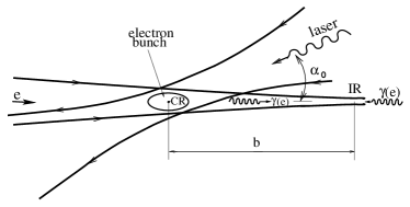
Figure 1: Scheme of PLC

The well-known scheme of   PLC is shown in Fig. 1. In the conversion region $CR$ preceding the interaction region $IR$, electron ($e^{-}$ or $e^{+}$) beam of the LC encounters a photon beam (a flash of a powerful laser). The Compton scattering of laser photon on electron from LC (with energy $E$) generates a photon with energy close to $E$,

$$e_{o}\gamma_{o}\to e\gamma\,.$$ (2)

These photons are focused in the IR into a spot of about the same size as expected for electrons without laser conversion. In the IR these photons collide with photons from the opposite conversion region ($\gamma\gamma\,$collisions) or with electrons from counter-propagating beam ($\gamma e$ collisions).

The ratio of the number of high energy photons to that of electrons in LC is called the conversion coefficient $k$, for the standard PLC $k\approx 1-1/e\approx 0.63$ typically.

Numerous studies of PLC (see, for example, [10], [11], [15]) are developing many new technical details, but they all retain the original scheme of Fig. 1.

The main properties of the basic Compton process are determined by the parameter

$$x=4E\omega_{0}/m_{e}^{2}\,,$$ (3)

where $E$ is the electron beam energy and $\omega_{0}$ – the laser photon energy. (To simplify text, we set $\alpha_{0}=0$ in Fig. 1.)

In 1981, to construct PLC, it was proposed to use a laser with neodymium glass or garnet, for which $\omega_{o}=1.17$ eV [7]-[8]. For electrons with energy $E\leqslant 250$ GeV, this choice remains optimal until now. Using such a laser, we have

$$\begin{gathered}2E=0.5\;TeV\;\Rightarrow\;x=4.5;\\ 2E=1\;TeV\;\Rightarrow\;x=9;\\ 2E=2\;TeV\;\Rightarrow\;x=18;\\ 2E=11\;TeV\Rightarrow\;x=100.\end{gathered}$$ (4)

First three lines here correspond different stages of ILC and CLIC projects, the fourth line represents some aymptotics.

$\bullet$  The described scheme in its pure form works only at $x<2(1+\sqrt{2})=4.8$ (at $E<270$ GeV for mentioned laser). At higher values of $x$, which will be realized at the subsequent stages of ILC, CLIC,…, some of the resulting high-energy photons die out, forming the $e^{+}e^{-}\,$pairs in collisions with laser photons from the tail of a laser flash,

$$\gamma\gamma_{o}\to\mbox{$e^{+}e^{-}\,$}\quad(killing\;\;process)\,.$$ (5)

This fact was considered as limiting the possibility of implementing a PLC based on LC with high electron energies [7], [8]).

Two ways to overcome this difficulty are discussed.
(1) To use a new laser with lower photon energy, keeping $x\lesssim 4.8$;
(2) To use existing laser, resigned to the decrease in $\gamma\gamma\,$ luminosity.

$\triangledown$ The results of [7] – [9] are directly applicable for the first way. However, a new laser is required for each new energy of electrons; so far, such lasers with the required parameters have not been developed.

$\triangledown$ , This work is devoted to the study of the second way with the guiding idea to get almost monochromatic collisions of photons at a cost an acceptable decrease in luminosity. This possibility is noted in [22, 23] and partially developed in [22].

Unfortunately, the method of optimizing the conditions for conversion $e\to\gamma$ used in [22] gives an inaccurate result for some beam polarizations. The analysis of the spectra of final photons without considering the polarization of particles distorts the spectra and the luminosity distribution. The result is obtained only for a certain configuration of the facility. It is not clear what changes should be expected when the engineering solution for beam collision changes. We correct these inaccuracies below and find out to what extent the results can be applied to any engineering solution for beam collisions. We call such photon collider the TeV PLC.

$\bullet$  Desirability of magnetic deflection of the electrons along the CR–IR path. In the papers [7]-[9] it was proposed to remove electrons that survived after conversion from the interaction region using a transverse magnetic field along the CR - IR path. For $x<4.8$, the problem was to obtain the maximum conversion coefficient so that after passing through the CR, only a small part of the electrons retained their initial energy, and most of electrons decrease energy and scatter away at small angles, similar to photons. This effect increased the total spread of electrons in the transverse plane. In addition, when using colliding $e^{-}e^{-}$ beams, residual electrons in the IR are repulsed by Coulomb forces so that the interaction of these electrons with each other and with the resulting photon beams becomes insignificant. Therefore, it is possible to dispense with the inclusion of this magnetic field [10]. The PLC projects discussed in [11]-[16] do not have such a magnetic field.

For $x>4.8$, in the optimal situation (see below), about one half of the electrons pass through the CR freely (without interaction with photons). In the absence of a magnetic field, it would be wrong to neglect their interaction with counterpropagating photons and electrons. To eliminate this interaction, electrons must be removed from the interaction region using a transverse magnetic field along the CR-IR path, as it was suggested in [7]-[9]. Further, we assume for $\boldsymbol{x>4.8}$ that when studying $\gamma\gamma\,$ collisions the magnetic field is turned on for both beams, and when studying $e\gamma\,$ collisions the magnetic field is turned on for one beam (converted to photon).

$\bullet$  The organization of the subsequent text is as follows.

Section 2 contains basic notation and a description of the Compton process in the studied parameter range with examples for $x=4.5$. We also introduce the important concept of the optical length of a laser flash for high-energy electrons.

In Section 3, we discuss the sources of photons falling into the interaction region. It is shown that the energy spectrum of these photons and the corresponding luminosities are naturally divided into two parts that are well separated from each other. The high- energy part, which is most interesting for studying the problems of New Physics, admits a universal description independent of the details of the experimental facility. There is no such universal description for the low-energy part. The basic notations related to the distribution of high-energy luminosity are also introduced in this section.

In the main part of the work (Section 4), we discuss the case $x>4.8$ and the main characteristics of high-energy $\gamma\gamma\,$and $e\gamma\,$collisions considering the modifications introduced by new processes in CR. We consider the cases $x=9,\;18$ (ILC, CLIC) in detail and give some examples for $x=100$. After a brief discussion of the basic Compton effect at $x>4.8$ (Section 4.1), Section 4.2 discusses the killing process $\gamma\gamma_{o}\to\mbox{$e^{+}e^{-}\,$}$, which was not discussed in necessary detail earlier, because it takes place only for $x>4.8$. In section 4.3 we write down the balance equations for the number of photons, produced in the Compton process and lost within the conversion region due to the killing process. The polarizing properties of the killing process turned out to be very significant.

The next step is to choose the optimal value for the laser flash energy or, in other words, the optical length of the laser flash. We have chosen as a criterion to obtain the maximum number of collided photons for the physics problems of interest (Section 5).

Section 6 contains a description of the resulting high-energy spectra for $e\gamma\,$ and $\gamma\gamma\,$ collisions.

A brief description of the results is given in Section 7.

In appendix A.1 we discuss the case of “bad” choice of initial polarization. In appendix   A.2 we find out that research with linear polarization of a high-energy photon is practically impracticable at TeV PLC. The most important background is discussed in appendix A.3. In appendix   A.4 we discuss the Bethe–Heitler process that could reduce the number of produced photons and show that this phenomenon is insignificant up to very high energies.

In appendix B, we list some of the important New Physics problems that can be explored using TeV PLC and cannot be studied using the LHC and $e^{+}e^{-}\,$colliders

2 Some notations, Compton effect on a high-energy electron

For definiteness, we consider as a base the $e^{-}e^{-}$ LC (not $e^{+}e^{-}$). We neglect the effects of high photon density in the conversion region (nonlinear QED effects). In all discussions, we assume $E\gg\omega_{o}$.

1. Notations.

• $\gamma_{o}$, $\omega_{o}$, $\lambda_{o}$ – the laser photon, its energy and helicity;

• $e_{o}$, $E$, $\lambda_{e}$ – the initial electron, its energy and helicity ($2|\lambda_{e}|\leqslant 1$);

• $\gamma$, $\omega$, $\lambda$ – the produced photon, its energy and helicity;

• $\sigma_{0}=\pi r_{e}^{2}=\;2.5\cdot 10^{-25}\;\mbox{cm}^{2}$;

• $b$ – the distance between the conversion region $CR$ and the interaction region $IR$ (Fig. 1);

• $\Lambda_{C}=2\lambda_{e}\lambda_{o}$ – polarization parameter of the process;

• $y=\omega/E$ – relative photon energy;

• $y_{M}=x/(x+1)$ – maximal value of $y$ at given $x$;

• $y_{\min}$ — position of the minimum in the dependence $d\sigma/dy$ on $y$ for the Compton process at $\Lambda_{C}\approx-1$ (defined for $x\geqslant 3$, it depends on $x$);

• $w_{\gamma\gamma}=\dfrac{{\sqrt{4\omega_{1}\omega_{2}}}}{{2E}}\equiv\sqrt{y_{1}y_{2}}\leqslant y_{M}$,
  $w_{e\gamma}=\dfrac{{\sqrt{4E\omega_{1}}}}{{2E}}\equiv\sqrt{y_{1}}\leqslant\sqrt{y_{M}}$ – ratios of the $\gamma\gamma\,$  and $e\gamma\,$ cms energies to $\sqrt{s}=2E$.

2. Compton scattering. We present the basic information about the Compton backward scattering in the kinematic region of interest according [7] – [9] in the form, suitable for description of high energy part of spectra at large $x$, with addition of some details which were not discussed earlier. Here numerical examples are given for $x=4.5$, which is close to the upper limit of validity in previous studies.

The total cross section of Compton effect is well known (Table 1):

$$\begin{gathered}\sigma_{C}=\dfrac{{2\sigma_{0}}}{{x}}\left[F(x)+\Lambda_{C}T(x)\right],\\ F(x)\!=\!\left(1-\dfrac{{4}}{{x}}\!-\!\dfrac{{8}}{{x^{2}}}\right)\ln(x+1)\!+\!\dfrac{{1}}{{2}}\!+\!\dfrac{{8}}{{x}}\!-\!\dfrac{{1}}{{2(x+1)^{2}}},\\ T(x)\!=\!\left(1\!+\!\dfrac{{2}}{{x}}\right)\ln(x+1)\!-\!\dfrac{{5}}{{2}}\!+\!\dfrac{{1}}{{x+1}}\!-\!\dfrac{{1}}{{2(x+1)^{2}}}.\end{gathered}$$ (6)

$x$	4.5	9	18	100
$\Lambda_{C}\!=\!-1$	0.73	0.45	0.26	0.056
$\Lambda_{C}=1$	0.85	0.63	0.44	0.145

Table 1: Compton cross section $\sigma_{C}/\sigma_{0}$ at different $x$ and $\Lambda_{C}$

The photon energy is kinematically bounded from above by quantity $y_{M}=x/(x+1)$ ($y_{M}=0.82$ for $x=4.5$). The energy distribution of photons strongly depends on $x$ and $\Lambda_{C}$ (here $r=\dfrac{{y}}{{x(1-y)}}\leqslant 1$)

$$\begin{gathered}f(x,y)\!\equiv\!\dfrac{{1}}{{\sigma_{C}}}\,\dfrac{{d\sigma_{C}}}{{dy}}=\dfrac{{U(x,y)}}{{F(x)+\Lambda_{C}T(x)}}\,,\\ U(x,y)=\dfrac{{1}}{{1-y}}+1-y-4r(1-r)-\Lambda_{C}xr(2-y)(2r-1).\end{gathered}$$ (7)

At $\Lambda_{C}\approx-1$, the photon spectrum grows up to its upper boundary $y=y_{M}$, at $\Lambda_{C}\approx 1$ this spectrum is much flatter (Figure 2).

At $x>3$ and $\Lambda_{C}\approx-1$ the high energy part of this distribution is concentrated in the narrow band below upper limit, contained more than one half produced photons. We characterize this band by its lower boundary $y_{\min}$ and the sharpness parameter $\tau$ – see Table 2

$$\begin{gathered}\!\!\mbox{\it alternative definition of $y_{\min}$:}\!\!\int\limits_{y_{\min}}^{y_{M}}\!\!f(x,y)dy\approx 0.55;\\ \mbox{\it definition of $\tau$:}f(x,y=y_{M}(1-\tau))\!=\!\dfrac{{1}}{{2}}\cdot f(x,y_{M}).\end{gathered}$$ (8)

x	4.5	9	18	100
$y_{\min}$	0.6	0.7	0.75	0.94
$\tau$	0.09	0.036	0.022	0.004

Table 2: Properties of high energy peak at $\Lambda_{C}\approx-1$

The mean circular polarization of the produced photon (helicity) is

$$\begin{gathered}\lambda(y)=\\ =\dfrac{{\lambda_{o}(1\!-\!2r)\left[\dfrac{{1}}{{1\!-\!y}}\!+\!1\!-\!y\right]\!+\!2\lambda_{e}xr[1\!+\!(1\!-\!y)(2r\!-\!1)^{2}]}}{{U(x,y)}}.\end{gathered}$$ (9a)

At $$\lambda_{o}=\pm 1$$, this equation is simplified:

$$\!\!\lambda(y)\!=\!-\!\lambda_{o}\left[(2r\!-\!\!1)\!+\!\dfrac{{\left[(2r\!-\!1)\!-\!\Lambda_{C}xr\right]4r(1-r)}}{{U(x,y)}}\right]\!.$$ (9b)

Maximum energy photons are well polarized with the same direction of spin as laser photons, i. e. $\lambda(y=y_{M})=-\lambda_{o}$.

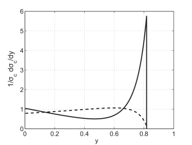
Figure 2: Photon energy spectrum $f(x,y)$ at $x=4.5$, $\Lambda_{C}=-1$ (solid) and $\Lambda_{C}=1$ (dotted)

These photons move in the direction of the initial electron. The emission angle of a photon increases as its energy decreases

$$\theta(y)=\dfrac{{m}}{{E}}\;\sqrt{x+1}\;\sqrt{\dfrac{{y_{M}}}{{y}}-1}.$$ (10)

Due to the increase in the angular spread on the way from the conversion region CR to the interaction region IR, softer photons are distributed over a wider region and collide less frequently than hard photons; their relative contribution to the luminosity decreases. As a result, the high-energy part of the resulting photon spectrum is better and better separated from the low-energy part as the distance $b$ increases together with decreasing total luminosity; this separation is enhanced with increasing energy $E$ of the colliding electrons.

3. The optical length of the laser bunch. The laser flash is assumed to be wide enough so that the inhomogeneity of the electron density inside the electron bunch is insignificant

The optical length of the laser bunch for electrons is expressed via the longitudinal density of photons in flash (i. e. via the laser bunch energy $A$ divided to its effective transverse cross section $S_{L}$) and the total cross section of the Compton scattering $\sigma_{C}(x,\Lambda_{C})$:

$$z=\dfrac{{A}}{{\omega_{o}S_{L}}}\,\sigma_{C}(x,\Lambda_{C})\equiv\dfrac{{A}}{{A_{0}}}\dfrac{{\sigma_{C}(x,\Lambda_{C})}}{{\sigma_{C}(x\!=\!4.5,\Lambda_{C}\!=\!-1)}}\,.$$ (11)

In the second form of this definition we introduce $A_{0}$ – the laser flash energy, necessary to obtain $z=1$ at $x=4.5$, $\Lambda_{C}=-1$.

When the electrons traverse the laser beam, their number decreases as

$$n_{e}(z)=n_{eo}e^{-z}\,.$$ (12)

3 Photons in the IR

Let us list the sources of photons in the interaction region.

The highest energies have photons produced in the main Compton effect. One can see that the number of such photons with energies greater than $y_{min}E$ is about 15% of the number of initial electrons after the loss of some of the photons in the killing process for $\Lambda_{C}\approx-1$ and for moderate distances from the conversion region to the interaction region under optimal conversion conditions (see below).

In addition, a significant number of photons of a different origin cross the interaction region.

(A) Photons produced from the scattering of the tail of the laser pulse (i) on electrons, which slow down in the main Compton effect (rescattering) or (ii) on positrons (electrons) produced in the killing process. These photons primarily had lower energies, and their angular distribution is wider than that of the initial Compton photons.

(B) Photons produced from magnetic lenses focusing beams and from synchrotron radiation with magnetic deflection of beams along the CR-IR beam path. Almost all of these photons have energies lower than $y_{min}E$.

(C) Photons produced from the interaction of electrons with each other, which survived in conversion (beamstrahlung). When using magnetic deflection, the number of such photons with energy greater than $y_{min}E$ is small.

$\bullet$   Two regions in the energy distribution. Thus, the luminosity spectrum of $\gamma\gamma\,$collision is naturally divided into two regions: (i) a high-energy region for $w>y_{min}E$ and (ii) a low-energy region for lower values $w$. These regions are well separated from each other.

The magnitude and shape of the low-energy luminosity obviously depend on the details of the experimental facility. They are not discussed in this work.

$\bullet$  High-energy luminosity and selection of events. For the problems of New Physics high-energy photons with $\omega\sim E$ are important. We study the high-energy luminosity only, considering the selection of events, which include the states with total energy $\varepsilon>E_{lim}\sim E$. This part of the luminosity spectrum is formed by photons produced in the main Compton effect (2), some of them disappear in the killing process (5).

$\bullet$  Luminosities. We consider relative luminosities $\cal L$, and high energy luminosity integral

$$\begin{gathered}L_{\rm exp}(w)={\cal L}(w)\cdot L_{\rm geom},\\ {\cal L}_{\rm h.e.}=\!\!\int\limits_{y_{\min}}^{1}\!\!{\cal L}(w)dw\;\;\left(w=w_{e\gamma}\;\;or\;\;w_{\gamma\gamma}\right).\end{gathered}$$ (13)

Here $L_{\rm geom}$ is the luminosity of the $e^{-}e^{-}$ collider designed for $\gamma\gamma\,$ mode. In a nominal ILC option, i.e. at the electron beam energy of 250 GeV, the geometric luminosity can reach $L_{\rm geom}=12\cdot 10^{34}$ cm^-2s^-1 which is about 4 times greater then the anticipated $e^{+}e^{-}\,$luminosity.

All subsequent calculations are performed for the case of a "good" polarization of collided electrons and photons $\Lambda_{C}\approx-1$ for high energy part of luminosity, in two versions: $\Lambda_{C}=-1$ and $\Lambda_{C}=-0.86$.

We discuss luminosities $L_{I}$ for different values of the total helicity $I=|\lambda_{1}-\lambda_{2}|$ of initial state (these are $L_{1/2}$ and $L_{3/2}$ for $e\gamma\,$collisions, and ($L_{0}$ and $L_{2}$ for $\gamma\gamma\,$ collisions). We found that one of these helicities dominates in the high energy part of the luminosity spectrum. Therefore, below we discuss total luminosity (sum over both finite helicities) and indicate the contribution to it from states with non-leading complete helicity.

In addition to notations, listed in the Section 2, we also define quantities that depend on $x$, $\Lambda_{C}$ and $b$:
$\bullet$ ${\cal L}_{h.e.}$ — total luminosity of the high energy peak (13);
$\bullet$ $L_{m}=L(w_{M})$ – the maximal value of $L(w)$;
$\bullet$ $w_{M}$ – position of maximum in the dependence $L(w)$;
$\bullet$ $w_{\pm}$ – solutions of equation $L(w_{\pm})=L_{m}/2$;
$\bullet$ $\gamma_{w}=(w_{+}-w_{-})/w_{M}$ – relative width of obtained peak;
(For $e\gamma\,$ mode $w_{+}=w_{m}=\sqrt{y_{M}}$, $L_{m}$ don’t depend on the distance $b$,$\gamma_{w}=1-w_{-}/w_{M}$.)

Luminosities of $\gamma\gamma\,$and $e\gamma\,$collisions are given by the convolution of the spectrum of a high-energy photon with the spectrum of a counter-propagating photon or electron, considering in the calculations transverse widening of the photon beam on the way from the conversion region CR to the interaction region IR. Real beams of electrons in LC are elliptical in the transverse direction; we denote by $\sigma_{x}$ and $\sigma_{y}$ the semi-axes of the ellipse in the interaction region. This ellipticity does not allow to use formulas from [7]–[9], and for each discussed CR–IR configuration, a new simulation is usually performed (for example, see [10]–[16]).

$\bullet$  Simple parameterization. In [25], we found that (only at $y>y_{min}$) the effect of beam broadening on the way CR–IR is described with good accuracy by a single parameter (as for a round beam)

$$\rho^{2}=\left(\dfrac{{b}}{{(E/m_{e})\sigma_{x}}}\right)^{2}+\left(\dfrac{{b}}{{(E/m_{e})\sigma_{y}}}\right)^{2}\,.$$ (14)

In other words, the shape of the high-energy part of the luminosity distribution is determined in an universal way regardless of the details of experimental facility.

In this approximation, the discussed luminosities are expressed via distributions in the photon energy by formulas, where $\phi_{a}=\sqrt{y_{M}/y_{a}-1}$ and $I_{0}(z)$ is the modified Bessel function, [7] – [9]:

$$\dfrac{{dL_{\gamma e}^{\lambda}}}{{dy}}=n_{e}n_{\lambda}(y,z)e^{-\dfrac{{\rho^{2}\phi^{2}}}{{2}}}\,;$$ (15)

$$\!\!\!\!\dfrac{{dL_{\gamma\gamma}^{2,\lambda_{1}\lambda_{2}}}}{{dy_{1}dy_{2}}}\!=\!n_{\lambda_{1}}(y_{1},z)n_{\lambda_{2}}(y_{2},z)I_{0}(\rho^{2}\phi_{1}\phi_{2})e^{-\,\dfrac{{\rho^{2}(\phi_{1}^{2}+\phi_{2}^{2})}}{{2}}}\,.$$ (16)

The distributions over the center of mass energy $w$ are obtained by the substitution $w=\sqrt{y}$  for $e\gamma\,$ luminosity or $w=\sqrt{y_{1}y_{2}}$ with simple integration, for $\gamma\gamma\,$ luminosity.

At $x\leqslant 4.8$ each lost electron produces the photon. Therefore at $z=1$ and $\rho=0$   total $e\gamma\,$ and $\gamma\gamma\,$ luminosities are

$${\cal L}_{e\gamma}=(1-1/e)=0.63\,,\quad{\cal L}_{\gamma\gamma}=(1-1/e)^{2}=0.4.$$ (17)

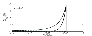
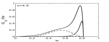
Figure 3: Luminosity spectra $dL/dw$ at $x=4.5$, $\Lambda_{C}=-1$, $z=1$ for $\rho=1$ (up) and $\rho=5$ (down) – solid lines, dotted lines – similar distributions at $\rho=1$ for final states with total helicity $3/2$ for $e\gamma\,$ collisions (left figure) and total helicity 2 for $\gamma\gamma\,$ collisions (right figure).

Fig. 3 and first lines of Tables 4, 5 represent $\gamma\gamma\,$  and  $e\gamma\,$ luminosity distributions in their cms energy at $z=1$, $\Lambda_{C}=-1$ for $\rho=1$ and 5.

4 What happens at $\boldsymbol{x\geqslant 4.8}$

4.1 Basic spectra

The photon energy spectrum for the basic Compton backscattering (7) at $x=9$ is shown in Fig. 4 – top panel. It can be seen that this spectrum for $\Lambda_{C}=-1$ is concentrated near the high energy limit strongly then the corresponding spectrum for $x=4.5$ in Fig. 2. At $x=18$ similar calculations reveals that the spectrum is concentrated in the band $0.85<y\equiv\omega/E<0.95$.

At $\Lambda_{C}=1$ spectrum is almost flat, with a minimum instead of a peak near the upper boundary.

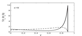
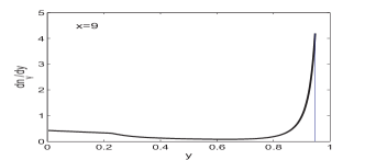
Figure 4: The case $x=9$. Left panel – Compton spectrum of photons. Solid line corresponds to $\Lambda_{C}=-1$, dashed line – to $\Lambda_{C}=1$. Right panel – photon energy spectrum reduced by killing process at $\Lambda_{C}=-1$, $z=0.7$

4.2 Killing process $\gamma\gamma_{o}\to\mbox{$e^{+}e^{-}\,$}$

The killing process is responsible for the disappearance of the Compton high-energy photons in their collisions with laser photons from the tail of a bunch, generating $e^{+}e^{-}\,$ pairs, this process is switches on at $x\approx 4.8$.

For a photon with energy $yE$ the squared cms energy for killing process is $w^{2}_{k}=4\omega\omega_{o}/m_{e}^{2}=xy>4$. Its cross section is

$$\begin{gathered}\sigma_{\rm kill}(w^{2}_{k},\lambda_{o}\lambda)=\dfrac{{4\sigma_{0}}}{{w^{2}}}\Phi_{\mbox{$\gamma\gamma\,$}}(w^{2}_{k},\lambda_{o}\lambda)\,,\\ \Phi_{\mbox{$\gamma\gamma\,$}}(w^{2}_{k},\lambda_{o}\lambda)=\left(1+\dfrac{{4}}{{w^{2}_{k}}}-\dfrac{{8}}{{w^{4}_{k}}}\right)L-\\ -\left(1+\dfrac{{4}}{{w^{2}_{k}}}\right)v-\lambda_{o}\lambda(L\!-\!3v),\\ v=\sqrt{1-4/w^{2}_{k}\;},\quad L=2\ln\left(\dfrac{{w_{k}}}{{2}}(1+v)\right)\,.\end{gathered}$$ (18)

Note that $\sigma_{\rm kill}(\lambda_{o}\lambda>0)<\sigma_{\rm kill}(\lambda_{o}\lambda<0)$ at $w^{2}_{k}<15$. This inequality changes sign at $w^{2}_{k}>15$.

4.3 Equations

The balance of the number of high energy photons is given by their production in the Compton process (2) and their disappearance at the production of $e^{+}e^{-}\,$ pairs in the killing process (5).

Let us denote by $n_{\gamma}(y,z,\lambda)$ the flux of photons (per 1 electron) with the energy $yE$ and polarization $\lambda$ after travelling inside the laser beam with the optical length $z$. For calculations, it is convenient to split this flux into the sum of fluxes of right polarized photons $n_{(\gamma+)}(y,z)$ and left polarized photons $n_{(\gamma-)}(y,z)$ so that the total photon flux $n_{\gamma}(y,z)$ and its average polarization $\lambda$ are written as

$$\begin{gathered}n_{\gamma}(y,z)=n_{(\gamma+)}(y,z)+n_{(\gamma-)}(y,z),\\ \langle\lambda(y,z)\rangle=\dfrac{{n_{(\gamma+)}(y,z)-n_{(\gamma-)}(y,z)}}{{n_{(\gamma+)}(y,z)+n_{(\gamma-)}(y,z)}}\,.\end{gathered}$$ (19)

Naturally, $\langle\lambda(y,z\to 0)\rangle\to\lambda(y)$ from (9).

The variation of in these fluxes during the passage through a laser beam is described by the equations

$$\begin{gathered}\dfrac{{dn_{(\gamma\pm)}(y,z)}}{{dz}}=\\ =\!\dfrac{{1}}{{2}}\left(1\pm\lambda(y)\right)f(x,y)n_{e}(z)-n_{(\gamma\pm)}\dfrac{{\sigma_{\rm kill}(xy,\pm\lambda_{o})}}{{\sigma_{C}(x)}}.\end{gathered}$$ (20)

The number of photons and their mean polarization are expressed via auxiliary quantities $\nu_{\pm}$:

$$\begin{array}[]{c}n_{\gamma\pm}(y,z)=f(x,y)\nu_{\pm}(z,y),\quad\langle\lambda\rangle=\dfrac{{\nu_{+}(z,y)-\nu_{-}(z,y)}}{{\nu_{+}(z,y)+\nu_{-}(z,y)}}.\end{array}$$

The equation (20) is easily solved:

$$\begin{gathered}n_{(\gamma\pm)}(y,z)=f(x,y)n_{e0}\nu_{\pm}(y,z);\\ \mbox{where}\;\;\nu_{\pm}(y,z)=\dfrac{{\left(1\pm\Lambda_{C}(y)\right)}}{{2}}\cdot\dfrac{{e^{-\zeta_{\pm}z}-e^{-z}}}{{1-\zeta_{\pm}}};\\ \zeta_{\pm}=\dfrac{{\sigma_{\rm kill}(xy,\pm\lambda_{o})}}{{\sigma_{C}(x)}}\,.\end{gathered}$$ (21)

It is useful for future discussions to define in addition ratio of number of killed photons to the number of photons, prepared for the $\gamma\gamma\,$ collisions, $r_{K}(y,z)$ – Table 3.

In Fig. 4, we compare the energy spectrum of Compton photons (top panel) with what remains after the passage of a laser beam with an optical length $z=0.7$ (bottom panel). One can see that

(i) The shape of high-energy part of the spectrum is very similar to that for the pure Compton effect. (This similarity is due to the special relationship between the spin structures of processes (2) and (5). Neglecting this structure for process (5), as it was done in [22], one arrives at an erroneous conclusion about a strong <<sharpening>> of the resulting spectrum.)

(ii) The killing process <<eats>> away photons from the middle part of the energy spectrum (improving the separation of the high-energy and low-energy parts of the spectrum).

(iii) The separation of the high-energy and low energy parts of the spectrum increases with increasing $\rho$.

(iv) The part of the spectrum corresponding to $xy<4$ is relatively enhanced, since there is no killing process with these $xy$.

5 Optimization

At $x<4.8$, an increase in the optical length of the photonic target leads to a monotonic (but limited) rise in the number of photons (with a simultaneous increase in the background). At $x>4.8$, the killing process stops this rise, and for very large $z$, it kills almost all high-energy photons.

The dependence of the number of photons $n(y,z)$ on $z$ has a maximum for some $z=z_{m}(y)$. This can be interpreted as the optimal value of $Z$. There is a question: what criterion should be used for the optimal choice?

The simplest approach is to consider this balance only for photons of maximal energy, at $y=y_{M}$ [22]. We find it more reasonable to consider for this goal the $z$-dependence of entire luminosity within its high energy peak ${\cal L}_{h.e.}$ (13), (8), Table 2.

(At $\Lambda_{C}\approx-1$, the photon energy spectra are concentrated in the narrow band near $y=y_{M}$. Therefore, the results of both optimizations are close to each other. At $\Lambda_{C}=1$ the initial spectra are flat, and the estimates made for $y=y_{M}$ [22] give an unsatisfactory description of the luminosity.)

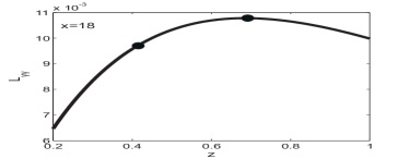
Figure 5: The $\gamma\gamma\,$ luminosity integral ${\cal L}_{h.e.}$ in dependence on $z$, for $\rho=1$, $\Lambda_{C}=-1$. Dots correspond $z_{m}$ and $z_{0.9}$.

A typical dependence of luminosity ${\cal L}_{h.e.}$ on $z$ is shown in Fig. 5. The curves at another $x$ and $\rho$ have similar form. The optimal value of the laser optical length are given by the position of a maximum at these curves, $z_{m}$. We found numerically that the value of $z_{m}$ is practically independent of $\rho$. These values at $\Lambda_{C}=-1$ and different $x$ are given in table 3. In addition to $z_{m}$, we include here the value $z_{0.9}(x)<z_{m}(x)$, provided luminosity which is 10% lower than maximal luminosity. In addition, this Table contains the energy of the laser flash $A$ (11) necessary to obtain these optical lengths (in terms of the energy of the laser flash $A_{0}$ needed to obtain $z=1$ for $x=4,5$); the fraction of photons spent on the production of $e^{+}e^{-}\,$ pairs, among photons with highest energy, generated in the basic Compton effect $r_{K}(z,y_{M})$ (obtained numerically); fraction of electrons freely passing through the laser bunch $d(z)=e^{-z}$.

x	$y_{\min}$	z	$A(z)/A_{0}$	$r_{K}(z,y_{M})$	d(z)
9	0.7	$z_{m}=0.704$	1.15	0.22	0.495
		$z_{0.9}=0.49$	0.8	0.13	0.61
18	0.75	$z_{m}=0.609$	1.70	0.43	0.54
		$z_{0.9}=0.418$	1.17	0.28	0.66
100	0.94	$z_{m}=0.48$	6.3		0.62
		$z_{0.9}=0.32$	4.2		0.73

Table 3: Numbers related to optimization at $\Lambda_{C}=-1$:

6 Luminosity distributions

Figure. 6 presents spectra of high energy luminosity for $\gamma\gamma\,$ and $e\gamma\,$ collisions at $x=18$, $\Lambda_{C}=-1$ for $z=z_{m}$ $\rho=1$ and 5. (The curves for other $x$ and $\rho$ look similar.) The tables 4 and 5 represent properties of these luminosity spectra at $x=9$ and $18$ for $\Lambda_{C}=-1$ and $\Lambda_{C}=-0.86$ at $z=z_{m}$. (The table rows for $x=4.5$, $z=1$ and $x=100$, $z=z_{m}$ are presented for comparison.)

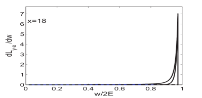
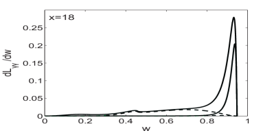
Figure 6: Luminosity spectra $dL/dw$ at $x=18$, $\Lambda_{C}=-1$, $z=1$ for $\rho=1$ (upper curves) and $\rho=5$ (lower curves) – solid lines; dotted lines – similar distributions for final states with total helicity $3/2$ ($\gamma e$) or 2 ($\gamma\gamma\,$) at $\rho=1$.

$\rho$	$\Lambda_{C}$	${\cal L}_{h.e.}$	$L_{2}/L$	$L_{m}$	$w_{M}$	$w_{-}$	$w_{+}$	$\gamma_{w}$
$\mbox{$\gamma\gamma\,$}:\qquad x=4.5,\qquad z=1,\;\;$
$\begin{array}[]{c}1\\ \\ 5\end{array}$	$\begin{array}[]{c}-1\\ -0.86\\ \hline\cr-1\\ -0.86\end{array}$	$\begin{array}[]{c}0.121\\ 0.114\\ 0.031\\ 0.0275\end{array}$	$\begin{array}[]{c}0.143\\ 0.215\\ 0.041\\ 0.086\end{array}$	$\begin{array}[]{c}0.933\\ 0.82\\ 0.464\\ 0.40\end{array}$	$\begin{array}[]{c}0.779\\ 0.778\\ 0.799\\ 0.7985\end{array}$	$\begin{array}[]{c}0.689\\ 0.672\\ 0.760\\ 0.0758\end{array}$	$\begin{array}[]{c}0.89\\ 0.809\\ 0.814\\ 0.813\end{array}$	$\begin{array}[]{c}0.154\\ 0.177\\ 0.067\\ 0.069\end{array}$
$\mbox{$\gamma\gamma\,$}:\qquad x=9,\qquad z=z_{m}=0.704,\;\;$
$\begin{array}[]{c}1\\ \\ 5\end{array}$	$\begin{array}[]{c}-1\\ -0.86\\ \hline\cr-1\\ -0.86\end{array}$	$\begin{array}[]{c}0.0214\\ 0.0201\\ 0.0072\\ 0.064\end{array}$	$\begin{array}[]{c}0.079\\ 0.164\\ 0.021\\ 0.074\end{array}$	$\begin{array}[]{c}0.222\\ 0.195\\ 0.137\\ 0.118\end{array}$	$\begin{array}[]{c}0.872\\ 0.871\\ 0.885\\ 0.885\end{array}$	$\begin{array}[]{c}0.814\\ 0.806\\ 0.854\\ 0.852\end{array}$	$\begin{array}[]{c}0.894\\ 0.894\\ 0.896\\ 0.896\end{array}$	$\begin{array}[]{c}0.092\\ 0.100\\ 0.048\\ 0.050\end{array}$
$\mbox{$\gamma\gamma\,$}:\qquad x=18,\qquad z=z_{m}=0.609,\;\;$
$\begin{array}[]{c}1\\ 5\end{array}$	$\begin{array}[]{c}-1\\ -0.86\\ \hline\cr-1\\ -0.86\end{array}$	$\begin{array}[]{c}0.0178\\ 0.0178\\ 0.0074\\ 0.069\end{array}$	$\begin{array}[]{c}0.089\\ 0.228\\ 0.021\\ 0.144\end{array}$	$\begin{array}[]{c}0.2615\\ 0.229\\ 0.190\\ 0.164\end{array}$	$\begin{array}[]{c}0.9317\\ 0.931\\ 0.9365\\ 0.936\end{array}$	$\begin{array}[]{c}0.8932\\ 0.886\\ 0.9138\\ 0.912\end{array}$	$\begin{array}[]{c}0.9436\\ 0.09436\\ 0.9447\\ 0.09447\end{array}$	$\begin{array}[]{c}0.054\\ 0.062\\ 0.033\\ 0.035\end{array}$
$\mbox{$\gamma\gamma\,$}:\qquad x=100,\qquad z=z_{m}=0.477,\;\;$
$\begin{array}[]{c}1\\ 5\end{array}$	-1	$\begin{array}[]{c}0.0093\\ 0.0070\end{array}$	$\begin{array}[]{c}0.017\\ 0.009\end{array}$	$\begin{array}[]{c}0.527\\ 0.519\end{array}$	$\begin{array}[]{c}0.9867\\ 0.9867\end{array}$	$\begin{array}[]{c}0.9771\\ 0.9793\end{array}$	$\begin{array}[]{c}0.9890\\ 0.9890\end{array}$	$\begin{array}[]{c}0.012\\ 0.0097\end{array}$

Table 4: Properties of high energy $\gamma\gamma\,$ luminosity for different $x$ and $\Lambda_{C}$.

$\rho$	${\cal L}_{h.e.}$	$L_{m}$	$L_{3/2}/L$	$\gamma_{w}$	${\cal L}_{h.e.}$	$L_{m}$	$L_{3/2}/L$	$\gamma_{w}$
$x=4.5,\qquad z=1,\qquad w_{M}=0.9045$
$\begin{array}[]{c}1\\ 5\end{array}$	$\begin{array}[]{c}0.38\\ 0.143\end{array}$	7.626	$\begin{array}[]{c}0.135\\ 0.007\end{array}$	$\begin{array}[]{c}0.0296\\ 0.0141\end{array}$	$\begin{array}[]{c}0.372\\ 0.134\end{array}$	7.034	$\begin{array}[]{c}0.182\\ 0.079\end{array}$	$\begin{array}[]{c}0.031\\ 0.014\end{array}$
	$\Lambda_{C}=-1$				$\Lambda_{C}=-0.86$
$x=9,\qquad z=0.7047,\qquad w_{M}=0.949$
$\begin{array}[]{c}1\\ 5\end{array}$	$\begin{array}[]{c}0.153\\ 0.074\end{array}$	4.837	$\begin{array}[]{c}0.069\\ 0.05\end{array}$	$\begin{array}[]{c}0.0176\\ 0.0105\end{array}$	$\begin{array}[]{c}0.149\\ 0.068\end{array}$	4.32	$\begin{array}[]{c}0.116\\ 0.063\end{array}$	$\begin{array}[]{c}0.018\\ 0.011\end{array}$
	$\Lambda_{C}=-1$				$\Lambda_{C}=-0.86$
$x=18,\qquad z=0.609,\qquad w_{M}=0.973$
$\begin{array}[]{c}1\\ 5\end{array}$	$\begin{array}[]{c}0.136\\ 0.08\end{array}$	7.015	$\begin{array}[]{c}0.0625\\ 0.0059\end{array}$	$\begin{array}[]{c}0.0098\\ 0.0070\end{array}$	$\begin{array}[]{c}0.138\\ 0.076\end{array}$	6.439	$\begin{array}[]{c}0.12\\ 0.077\end{array}$	$\begin{array}[]{c}0.01\\ 0.007\end{array}$
	$\Lambda_{C}=-1$				$\Lambda_{C}=-0.86$
$x=100,\qquad z=0.477,\qquad w_{M}=0.995$
$\begin{array}[]{c}1\\ 5\end{array}$	$\begin{array}[]{c}0.099\\ 0.083\end{array}$	22.905	$\begin{array}[]{c}0.0086\\ 0.0042\end{array}$	$\begin{array}[]{c}0.002\\ 0.0018\end{array}$	$\begin{array}[]{c}0.1085\\ 0.088\end{array}$	21.905	$\begin{array}[]{c}0.108\\ 0.103\end{array}$	$\begin{array}[]{c}0.002\\ 0.0018\end{array}$
	$\Lambda_{C}=-1$				$\Lambda_{C}=-0.86$

Table 5: Properties of high energy    $e\gamma\,$ luminosity for different $x$ and $\Lambda_{C}$.

Let us list the important properties of these distributions for $x=9$ and $18$:

(1) At the electron beam energy $E=1$ TeV, the maximal photon energy is $\omega_{m}=0.95$ TeV ($\sqrt{s_{\mbox{$\gamma\gamma\,$}}}\approx 1.9$ TeV).

(2) High-energy luminosity at $\rho=1$:
${\cal L}_{h.e.}^{\mbox{$\gamma\gamma\,$}}\approx 0.02L_{\rm{geom}}$ (annual $>10$ fb^-1), it is about $5.5$ times less than that for $x=4.5$; ${\cal L}_{h.e.}^{\mbox{$e\gamma\,$}}\approx 0.15L_{\rm{geom}}$, about 2.5 times less than that for $x=4.5$.

(3) Peak differential luminosity
$L_{m}^{\mbox{$e\gamma\,$}}(x=9)\approx L_{m}^{\mbox{$e\gamma\,$}}(x=4.5)$ and does not depend on $\rho$; $L_{m}^{\mbox{$\gamma\gamma\,$}}(x=9,\rho=1)\approx 0.25L_{m}^{\mbox{$\gamma\gamma\,$}}(x=4.5,\rho=1)$.

(4) As $\rho$ increases, the integrated luminosity and the peak value decrease, but this decrease is slower than for $x=4.5$.

(5) Photons within considered peaks are well polarized: at $\rho=1$ the fraction of luminosities ${\cal L}_{2}$ or ${\cal L}_{3/2}$ in the total luminosities is small; at $\rho=5$ these fractions are negligible.

(6) The energy distribution of luminosity is very narrow: for $\gamma\gamma\,$ collisions, the peak width is comparable to the peak width in the $e^{+}e^{-}\,$collision mode (considering the radiation in the initial state (ISR) and beam radiation (beamstrahlung, BS)). For $e\gamma\,$ collisions, the peak width is even narrower than in the basic $e^{+}e^{-}\,$collision (considering ISR and BS). The rapidities of produced $e\gamma\,$ and $\gamma\gamma\,$ systems in the collider rest frame are contained within a narrow intervals, determined by the spread of photon energies within high-energy peak (8),

$$\begin{gathered}\eta_{e\gamma}\in\left(\dfrac{{1}}{{2(x+1)}},\;\dfrac{{1}}{{2(x+1)}}+\bar{\tau}\right),\quad|\eta_{\gamma\gamma}|\leqslant\bar{\tau},\;\;with\;\;\bar{\tau}\approx\dfrac{{\tau}}{{2}}\,.\end{gathered}$$ (22)

(7) Imperfect polarization of the initial electrons $2\lambda_{e}=-0.86$ instead of $2\lambda_{e}=-1$ only weakly degrades the spectra.

7 Summary

(1) The LC with electron energy $E\leqslant 1$ TeV allows one to construct a photon collider (TeV PLC) using the same lasers and optical systems as those designed for construction PLC at $E\leqslant 250$ GeV. In comparison with that case, the required laser flash energy should be increased by no more than $70-20$%.

The total luminosity integral for high energy part of spectrum is high enough. In this part photon energies are very close to $E$, photons are monochromatic with good accuracy in both energy and polarization.

(3) For TeV PLC two complements compared to the $x<4.8$ case seem to be very desirable:

(a) the magnetic deflection of electrons after conversion (see page 1),

(b) the selection of events with total observed energy of reaction products $\varepsilon>E_{lim}\sim E$ (see page 5).

(4) The low-energy part of the photon spectrum in IR includes photons from different channels. It is highly dependent on the details of experimental facility. In some variants of this facility the corresponding luminosity can be large [31]. This part of spectrum can be used to study more traditional problems (for example, see [32]).

Appendix A Some background processes and related issues

A.1 A1. "Bad" initial helicity $\Lambda_{C}\approx 1$

At $\Lambda_{C}=1$ the photon spectrum in the main Compton process is much flatter than in the "good" case $\Lambda_{C}=-1$, see Fig. 2. Therefore, in estimates of integrated luminosity (13) one should use lower value $y_{\min}$, e.g. $y_{\min}=0.6$. The optimum optical length in this case is higher than that for the "good" case $\Lambda_{C}=-1$, in particular, $z_{m}(x=18,\,\Lambda_{C}=1)=0.827$, $z_{m}(x=100,\,\Lambda_{C}=1)=1.07$. This requires a laser flash energy that is not much higher than that for the <<good case>>, $A=1.43A_{0}$ for $x=18$ and $A=5.4A_{0}$ for $x=100$.

The more important difference is the shape of the luminosity spectrum. This spectrum is much flatter than one shown in Fig. 6. The position of its smeared maximum shifts toward much smaller values of $w$. Here an one-parametric description of the spectrum at the beam collisions (14)-(16) becomes invalid, details of device construction are essential. In this case, the separation between high-energy and low-energy parts of the luminosity spectrum is practically absent

With the growth of distance $b$ (Fig. 1) the low-energy part of luminosity disappears, the residual peak gives much lower integrated luminosity than that at $\Lambda_{C}\approx-1$.

A.2 A2. The linear polarization of high energy photon

The linear polarization of high energy photon is expressed via linear polarization of the laser photon $P_{\ell 0}$ by well known ratio $(N/D)$ (see [9]), in which $|N|\leqslant|2P_{\ell 0}|$ and $D\propto f(x,y)$. To reach maximal high energy luminosity in the entire spectrum, the denominator $D$ should be large. Therefore, the linear polarization of photon can be only small in the cases with relatively high $\gamma\gamma\,$luminosity. We cannot hope to observe these effects at the TeV PLCs under discussion.

A.3 A3. Collisions of positrons with electrons of the counter-propagating beam

Collisions of positrons from killing process with electrons of the opposite beam result in physical states similar to those produced in $\gamma\gamma\,$collisions. It will be the main background for TeV PLC.

General. According to Table 3, at $x=18$ and $z=z_{m}$ the number of killed photons producing high energy $e^{+}e^{-}\,$ pairs is less than 3/4 from the number of operative photons. This ratio decreases at lower $x$. Only one half from these photons produces high energy positrons. Therefore the luminosity of these collisions ${\cal L}_{b}(\mbox{$e^{+}e^{-}\,$})\lesssim(1.5\div 2.5){\cal L}(\mbox{$\gamma\gamma\,$})$.

$\lozenge$ The use of the optical length $z_{0.9}$ instead of the optimal one $z_{m}$ reduces number of positrons and ${\cal L}_{b}(\mbox{$e^{+}e^{-}\,$})$ by half or even more with a small change in the $L_{\mbox{$\gamma\gamma\,$}}$.

Energy distribution of positrons etc. The details of luminosity distribution of these $e^{+}e^{-}\,$collisions differ strongly from those for $\gamma\gamma\,$collisions of main interest. To verify this, consider the energy distribution of positrons produced by photons with energy $\omega=Ey$ and polarization $\lambda$. We use notations (18) and denote the positron energy by $E_{+}=y_{+}\omega$. The kinematic constraints are

$$\begin{gathered}w^{2}=sy\geqslant 4,\quad v=\sqrt{1-4/w^{2}},\quad\dfrac{{1+v}}{{2}}\geqslant y_{+}\geqslant\dfrac{{1-v}}{{2}},\end{gathered}$$ (23a)

so

$$\begin{gathered}y_{+}\leqslant 0.77\to E_{+}\leqslant 0.693E\;\;\mbox{at}\;\;x=9,\\ y_{+}\leqslant 0.888\to E_{+}\leqslant 0.841\;\;\mbox{at}\;\;x=18\,.\end{gathered}$$ (23b)

As a result, the rapidity of system produced in these $e^{+}e^{-}\,$collision is

$$\eta_{\mbox{$e^{+}e^{-}\,$}}(x=9)\geqslant 0.153,\quad\eta_{\mbox{$e^{+}e^{-}\,$}}(x=18)\geqslant 0.08.$$ (24)

These values don’t intersect with the possible rapidity interval for $\gamma\gamma\,$ system (22). Therefore, the $e^{+}e^{-}\,$and $\gamma\gamma\,$ events are clearly distinguishable in the case of observation of all reaction products.

In general, a more detailed description is desirable. The energy distribution of positrons produced in the $\gamma_{o}\gamma$ collision is

$$\begin{gathered}\dfrac{{dn_{+}(y_{+};w^{2},\lambda\lambda_{o})}}{{dy_{+}}}=\dfrac{{(u-2)(1+c\lambda_{o}\lambda)+s^{2}}}{{\Phi_{\mbox{$\gamma\gamma\,$}}(w^{2},\lambda_{o}\lambda)}};\\ u=\dfrac{{1}}{{y_{+}(1-y_{+})}},\quad c=2\dfrac{{u}}{{w^{2}}}-1,\quad s^{2}=1-c^{2}\,.\end{gathered}$$ (25)

For the highest positron energy $c=1$, and we have $dn=0$ (at $\lambda_{o}\lambda=-1$). This equality $dn=0$ corresponds to the fact that the angular momentum conservation forbids production of positrons (or electrons) in the forward direction. It means that the physical flux of positrons is limited even stronger than that given by Eq. (23).

Except mentioned endpoints, distribution (25) changes weakly in the whole interval of $y_{+}$ variation. Therefore, the $e^{+}e^{-}\,$luminosity is widely distributed over entire range of its possible variation. As a result, the differential luminosity $dL/dw_{\mbox{$e^{+}e^{-}\,$}}\ll dL/dw_{\mbox{$\gamma\gamma\,$}}^{peak}$.

Apart from the differences in the luminosity distribution, important differences in the produced systems at the same energies should be noted.

(i) With increasing energy all cross sections in $e^{+}e^{-}\,$mode decrease as $1/s$. In the $\gamma\gamma\,$mode cross sections of many processes don’t decrease.

(ii) In the $e^{+}e^{-}\,$mode most of processes are annihilation ones (via $\gamma$ or $Z$ intermediate states). Products of reaction in such processes have wide angular distribution. In the $\gamma\gamma\,$mode, a significant part of the reaction products move along the collision axis with a moderate transverse momentum.

A.4 A4. Bethe-Heitler process $\boldsymbol{e_{o}\gamma_{o}\to ee^{+}e^{-}}$

This process is switching on at $x=8$. It is the process of the next order in $\alpha$ but (in contrast to the Compton effect) its cross section does not decrease with growth of energy:

$\sigma_{BH}=(28/9\pi)\alpha\sigma_{0}(\ln x-109/42)\;\;$ at $x\gg 1$.

Because of this process, the yield of high-energy photons decreases by the factor

$$K_{BH}=\dfrac{{\sigma_{C}(x)}}{{\sigma_{C}(x)+\sigma_{BH}(x)}}\,,$$ (26)

and the $\gamma\gamma\,$ luminosity reduces by the factor $K_{BH}^{2}$. The numerical values of this factor are presented in the Table 6. It shows that the Bethe-Heitler mechanism is negligible at $x<100$, the reduction of the photon yield becomes unacceptably large at $x>300$.

$x$	30	100	300
$\Lambda_{C}=-1$	0.96	0.80	0.47
$\Lambda_{C}=1$	0.97	0.88	0.62

Table 6: Factor $K_{BH}$

Appendix B Some physical problems for TeV PLC

We expect LHC and $e^{+}e^{-}$ LC to yield many new results. Certainly, TeV PLC will complement these results and improve precision of some fundamental parameters. However, there are also important problems of fundamental physics that cannot be studied using the LHC and $e^{+}e^{-}\,$ colliders or require very great efforts to study, but they can find a solution using TeV PLC. We discuss just such problems below.

$\bullet$ Beyond Standard Model. In the extended Higgs sector one can realizes scenario, in which the observed Higgs boson $h$ is the SM-like (aligned) particle, while model contains others scalars which interact strongly. It was discussed earlier (for a minimal SM with one Higgs field) that physics of such strongly interacting Higgs sector can be similar to a low-energy pion physics. Such a system may have resonances like $\sigma$, $\rho$, $f$ with spin 0, 1 and 2 (by estimates, with mass $M\lesssim 1-2$ TeV). High monochromaticity of TeV PLC allows to observe these resonance states with spin 0 or 2 in $\gamma\gamma\,$ mode.

In the same manner one can observe excited electrons with spin 1/2 or 3/2 in $e\gamma\,$ mode.

$\bullet$ Gauge boson physics.

The SM electroweak theory is checked now at the tree level for simplest processes and at the 1-loop level for $Z$-peak. The ability to test the effects of this model in more complex processes and for off- peak loop effects look very important. A TeV PLC will provide us with a unique opportunity to explore these problems.

$\triangledown$ Processes  $\gamma\gamma\to WW$, $e\gamma\to\nu W$ have huge cross sections, by the standards of physics of TeV energies, at large $s$ we have [26, 27, 28, 29, 30]

$$\sigma(\gamma\gamma\to WW)\equiv\!\sigma_{V}\!=\!8\pi\alpha^{2}/M_{W}^{2}\!\approx\!86~{}pb,\;\sigma(e\gamma\to\nu W)\approx\left(\dfrac{{1}}{{2}}-\lambda_{e}\right)\sigma_{V}.$$ (27)

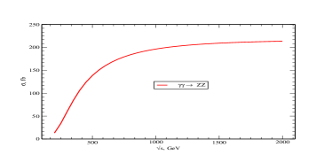
Figure 7: Cross sections for process $\mbox{$\gamma\gamma\,$}\to ZZ$ [30].

Therefore the measurement of these processes allows us to test the detailed structure of the electroweak theory with an accuracy about 0.1% (1-loop and partially 2-loop). To describe the results with such precision, a quantum field theory with unstable particles should be constructed.

With such precision, the sensitivity to possible anomalous interactions (operators of higher dimension) – that is, to the signals of BSM physics – will be enhanced [26]. The $\mbox{$\gamma\gamma\,$}\to ZZ$ and $\mbox{$\gamma\gamma\,$}\to\gamma Z$ processes will be the first well-measurable processes with variable energy, induced by only loop contributions [27], [29]. The energy dependence for the $\mbox{$\gamma\gamma\,$}\to ZZ$ cross section is shown in Fig. 7. Note that $\sigma(\mbox{$\gamma\gamma\,$}\to\gamma Z)\approx\sigma(\mbox{$\gamma\gamma\,$}\to ZZ)/3$. [30].

$\triangledown$ Processes with multiple production of gauge bosons at TeV PLC have relatively large cross sections, Fig. 8.

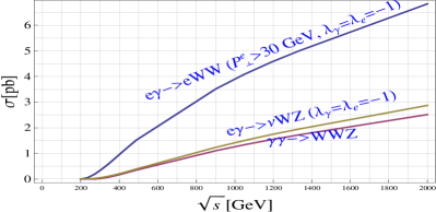
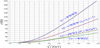
Figure 8: Cross sections of multiple production of gauge bosons, calculated with CalcHEP.

(For $e\gamma\,$ collisions we present$\sigma(\mbox{$e\gamma\,$}\to eWW)$, $\sigma(\mbox{$e\gamma\,$}\to eWWZ)$ for well observable transverse momenta of electrons $p_{\bot e}>30$ GeV.)

The relatively large values of these cross sections are due to the contribution of the diagrams with the exchange of vector bosons in the $t-$ channel, which does not decrease with increasing $s$ [33]. They grow logarithmically with factors $L\approx\ln(s/m_{e}^{2})$ for photon exchange or $\ell\approx\ln(s/M_{W}^{2})$ for $W(Z)$ exchange:

$$\begin{gathered}\sigma(\mbox{$e\gamma\,$}\to eWW)\sim\alpha\sigma_{W}L\,,\quad\sigma(\mbox{$e\gamma\,$}\to eWWZ)\sim\alpha^{2}\sigma_{W}L\ell\,,\\ \sigma(\mbox{$e\gamma\,$}\to\nu WW)\sim\alpha\sigma_{W}\ell\,,\quad\sigma(\mbox{$\gamma\gamma\,$}\to ZWW)\sim\alpha\sigma_{W}\ell\,,\\ \sigma(\mbox{$e\gamma\,$}\to\nu WWW)\sim\left[\sigma(\mbox{$\gamma\gamma\,$}\to WWZZ)/\sin^{2}\theta_{W}\right]\sim\alpha^{2}\sigma_{W}\ell^{2}\,,\\ \sigma(\mbox{$\gamma\gamma\,$}\to WWWW)\sim\alpha^{2}\sigma_{W}\ell^{2}/\sin^{4}\theta_{W}\,.\end{gathered}$$ (28)

These cross sections are sensitive to the details of gauge boson interactions (which cannot be seen in another way) and possible anomalous interactions. Nothing of the kind can be done on other colliders. Studying the dependence of $\mbox{$e\gamma\,$}\to eWW$, $\mbox{$e\gamma\,$}\to eWWZ$ cross sections on the electron transverse momentum will allow to measure the electromagnetic form factor $W$ in the processes$\gamma\gamma^{*}\to WW$, $\to WWZ$ and separate the contribution of processes $Z^{*}\gamma\to WW$, $Z^{*}\gamma\to WWZ$. The study of process $\mbox{$e\gamma\,$}\to\nu WZ$ allows to extract first information about subprocess $W^{*}\gamma\to WZ$.

$\bullet$ Hadron physics and QCD. Our understanding of hadron physics is twofold. We believe that we understand basic theory – QCD with its asymptotic freedom. However, the results of calculations in QCD can be applied to the description of data only with the aid of some phenomenological assumptions (often verified by long practice). It results in badly controlled uncertainties in the description of data.

$\triangledown$ PLC is to some extent the hadronic machine with more pure initial state than LHC. Therefore, PLC can be used also for detailed study of high energy QCD processes like diffraction, total cross sections, odderon, etc. The results of such experiments can be confronted to theory with much lower uncertainty than the corresponding ones at the LHC.

$\triangledown$ Studying the photon structure function $W_{\gamma}$ (in $e\gamma\,$ collision) will provide a unique QCD test. This function can be represented as the sum of point-like $W_{\gamma}^{pl}$ and hadronic $W_{\gamma}^{h}$ contributions. The hadronic part is similar to that for proton and is described by a similar phenomenology. On the contrary, the point-like contribution $W_{\gamma}^{pl}$ is described without phenomenological parameters [34]. The ratio $W_{\gamma}^{h}/W_{\gamma}^{pl}$ decreases with $Q^{2}$ roughly as $(\ln Q^{2})^{-1/3}$. In the range of parameters accessible today the hadronic contribution dominates. The point-like contribution should become dominant with $Q^{2}$ growth at TeV PLC.

References

- [1] L.D. Landau, E.M. Lifshitz. Sow. Phys. 6 (1934) 244
- [2] V.M. Budnev, I.F. Ginzburg, G.V. Meledin and V.G. Serbo. Phys. Rept. 15C (1975) 181.
- [3] V.E. Balakin, V.M. Budnev, I.F. Ginzburg. Pis’ma ZhetF 11 (1970) 559 ( ZhETF Lett. 11 (1970) 388);
- [4] V.M. Budnev, I.F. Ginzburg. Phys. Lett. 37B (1971) 320.
- [5] S. Brodsky, T. Kinoshita, H. Terazawa. Phys. Rev. Lett. 25 (1970) 972.
- [6] D. d’Enterria et al. PHOTON-2017 conference proceedings. arXiv:1812.08166
- [7] I.F. Ginzburg, G.L. Kotkin, V.G. Serbo and V.I. Telnov. ZhETF Pis’ma. 34 (1981) 514;
- [8] I.F. Ginzburg, G.L. Kotkin, V.G. Serbo and V.I. Telnov. Nucl. Instr. and Methods in Physics Research (NIMR) 205 (1983) 47.
- [9] I.F. Ginzburg, G.L. Kotkin, S.L. Panfil, V.G. Serbo and V.I. Telnov NIMR 219 (1983) 5.
- [10] V.I.Telnov. Problems of obtaining gamma-gamma and gamma-electron Colliding Beams at Linear Colliders.// Nucl. Instrum. Meth. A 294 (1990), 72-92
- [11] B. Badelek et al. Int. J. Mod. Phys. A 19 (2004) 5097-5186;
- [12] R.D. Heuer et al. TESLA Technical Design Report, p. III. DESY 2001-011, TESLA Report 2001-23, TESLA FEL 2001-05 (2001) p. 1–192 hep-ph/0106315.
- [13] B.Badelek et al. TESLA Technical Design Report. p. VI, chap.1 DESY 2001-011, TESLA Report 2001-23, TESLA FEL 2001-05 (2001) hep-ex/0108012, p.1-98;
- [14] M. Harrison, M. Ross, N. Walker, International Linear Collider. Technical Design report (2007-2010-2013). ArXiv:1308.3726 [hep-ph]
- [15] V.I. Telnov. Nuclear and Particle Physics Proceedings. 273–275 (2016) 219.
- [16] V.I. Telnov. ArXiv:1801.10471
- [17] P. Bambade et al. The International Linear Collider: A Global Project. ArXiv:1903.01629 [hep-ex]
- [18] CLIC and CLICdp collaborations. CERN Yellow Rep. Monogr. 1802 (2018);
- [19] A. Robson et al. The Compact Linear Collider (CLIC): Accelerator and Detector. ArXiv:1812.07987 [physics.acc-ph]
- [20] P. Roloff, R. Franceschini, U. Schnoor, A. Wulzer. The Compact Linear Collider (CLIC): Physics Potential. ArXiv:1812.07986 [hep-ex]
- [21] J. de Blas et al. The CLIC Potential for New Physics. ArXiv:1812.02093 [hep-ph].
- [22] V.I. Telnov. NIMR A 472 (2001) 280-290.
- [23] I.F. Ginzburg, G.L. Kotkin. Report at Photon 2009 (2009).
- [24] I.F. Ginzburg. ArXiv:0912.4841 [hep-ph].
- [25] I.F. Ginzburg, G.L. Kotkin. Eur. Phys. J. C 13 (2000) 295
- [26] I.F. Ginzburg, G.L. Kotkin, S.L. Panfil, V.G. Serbo. Nucl. Phys. B 228 (1983) 285 – 300. (E: B 243 (1984) 550).
- [27] G. Jikia, A.Tkabaladze. Pair Production at the Photon Linear Collider. Phys. Lett. B 332 (1994) 441;arXiv: hep-ph/9312274
- [28] G.Jikia. Electroweak gauge boson production at collider. Nucl. Phys. B405 (1993) 24, Phys. Lett. B298 (1993) 224; arXiv:hep-ph/9710459.
- [29] G.J. Gounaris, J. Layssac, P.I. Porfyriadis, F.M. Renard. The process and the search for virtual SUSY effects at a Collider. arXiv:hep-ph/9909243
- [30] L. Kalinovskaya, S. Bondarenko. Private communication (2020).
- [31] V.I. Telnov. Private communication (2013).
- [32] A. Abada et al. FCC Physics Opportunities. Eur. Phys. J. C79 (2019) 474
- [33] I.F. Ginzburg, V.A.Ilyin, A.E.Pukhov, V.G.Serbo, S.A.Shichanin. Rus. Yad. Fiz. 56 (1993) 57–63.
- [34] E. Witten. Nucl. Phys. B 120 (1977) 189.