Approximating Euclidean by Imprecise Markov Decision Processes

Abstract

Euclidean Markov decision processes are a powerful tool for modeling control problems under uncertainty over continuous domains. Finite state imprecise, Markov decision processes can be used to approximate the behavior of these infinite models. In this paper we address two questions: first, we investigate what kind of approximation guarantees are obtained when the Euclidean process is approximated by finite state approximations induced by increasingly fine partitions of the continuous state space. We show that for cost functions over finite time horizons the approximations become arbitrarily precise. Second, we use imprecise Markov decision process approximations as a tool to analyse and validate cost functions and strategies obtained by reinforcement learning. We find that, on the one hand, our new theoretical results validate basic design choices of a previously proposed reinforcement learning approach. On the other hand, the imprecise Markov decision process approximations reveal some inaccuracies in the learned cost functions.

1 Introduction

Markov Decision Processes (MDP) [12] provide a unifying framework for modeling decision making in situations where outcomes are partly random and partly under the control of a decision maker. MDPs are useful for studying optimization problems solved via dynamic programming and reinforcement learning. They are used in several areas, including economics, control, robotics and autonomous systems. In its simplest form, an MDP comprises a finite set of states $\mathcal{S}$, a finite set of control actions $\mathit{Act}$, which for each state $s$ and action $a$ specifies the transition probabilities $P_{a}(s,s^{\prime})$ to successor states $s^{\prime}$. In addition, transitioning from a state $s$ an action $a$ has an immediate cost $C(s,a)$. The overall problem is to find a strategy $\sigma$ that specifies the action $\sigma(s)$ to be made in state $s$ in order to optimize some objective (e.g. the expected cost of reaching a goal state).

For many applications, however, such as queuing systems, epidemic processes (e.g. COVID19), and population processes the restriction to a finite state-space is inadequate. Rather, the underlying system has an infinite state-space and the decision making process must take into account the continuous dynamics of the system. In this paper, we consider a particular class of infinite-state MDPs, namely Euclidean Markov Decision Processes [9], where the state space $\mathcal{S}$ is given by a (measurable) subset of $\mathbb{R}^{K}$ for some fixed dimension $K$.

As an example, consider the semi-random walk illustrated on the left of Fig. 1 with state-space $\mathcal{S}=[0,x_{max}]\times[0,t_{max}]$ (one dimensional space, and time). Here the goal is to cross the $x=1$ finishing line before $t=1$. The decision maker has two actions at her disposal: to move fast and expensive (cost $3$), or to move slow and cheap (cost $1$). Both actions have uncertainty about distance traveled and time taken. This uncertainty is modeled by a uniform distribution over a successor state square: given current state $(x,t)$ and action $a\in\{\mathit{slow},\mathit{fast}\}$, the distribution over possible successor states is the uniform distribution over $[x+\delta(a)-\varepsilon,x+\delta(a)+\varepsilon]\times[t+\tau(a)-\varepsilon,t+\tau(a)+\varepsilon]$, where $(\delta(a),\tau(a))$ represents the direction of the movement in space and time which depends on the action $a$, while the parameter $\varepsilon$ models the uncertainty. Now, the question is to find the strategy $\sigma:\mathcal{S}\rightarrow\mathit{Act}$ that will minimize the expected cost of reaching a goal state.

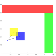
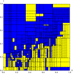
Figure 1: Left: a Semi-Random Walk on $\mathcal{S}=[0,1.2]\times[0,1.2]$. Green: goal area, red: failure area, blue dot: current state, yellow/blue squares: successor state squares for fast (blue) and slow (yellow) actions. Right: partition of $[0,1]\times[0,1]$ and strategy learned by UPPAAL STRATEGO; partition regions colored according to actions prescribed by the strategy.

In [9], we proposed two reinforcement learning algorithms implemented in UPPAAL STRATEGO [5], using online partition refinement techniques. In that work we experimentally demonstrated its improved convergence tendencies on a range of models. For the semi-random walk example, the online learning algorithm returns the strategy illustrated on the right of Fig. 1.

However, despite its efficiency and experimentally demonstrated convergence properties, the learning approach of [9] provides no hard guarantees as to how far away the expected cost of the learned strategy is from the optimal one. In this paper we propose a step-wise partition refinement process, where each partitioning induces a finite-state imprecise MDP (IMDP). From the induced IMDP we can derive upper and lower bounds on the expected cost of the original infinite-state Euclidean MDP. As a crucial result, we prove the correctness of these bounds, i.e., that they are always guaranteed to contain the true expected cost. Also, we provide value iteration procedures for computing lower and upper expected costs of IMDPs. Figure 2 shows upper and lower bounds on the expected cost over the regions shown in Figure 1.

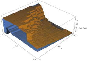
Figure 2: Lower and upper cost bounds for the learned partition.

Applying the IMDP value iteration procedures to the partition learned by UPPAAL STRATEGO therefore allows us to compute guaranteed lower and upper bounds on the expected cost, and thereby validate the results of reinforcement learning. The main contributions of this paper can by summarized as follows:

• We define IMDP abstractions of infinite state Euclidean MDPs, and establish as key theoretical properties: the correctness of value iteration to compute upper and lower expected cost functions, the correctness of the upper and lower cost functions as bounds on the cost function of the original Euclidean MDP, and, under a restriction to finite time horizons, the convergence of upper and lower bounds to the actual cost values.

• We demonstrate the applicability of the general framework to analyze the accuracy of strategies learned by reinforcement learning.

Related Work.

Our work is closely related to various types of MDP models proposed in different areas. Imprecise Markov Chains and Imprecise Markov Decision processes have been considered in areas such as operations research and artificial intelligence [15, 4, 14]. The focus here typically is on approximating optimal policies for fixed, finite state spaces. In the same spirit, but from a verification point of view, [2] focuses on reachability probabilities.

Lumped Markov chains are obtained by aggregating sets of states of a Markov Chain into a single state. Much work is devoted to the question of when and how the resulting process again is a Markov chain (it rarely is) [13, 6]. The interplay of lumping and imprecision is considered in [7] Most work in this area is concerned with finite state spaces. Abstraction by state space partitioning (lumping) can be understood as a special form of partial observability (one only observes which partition element the current state belongs to). A combination or partial observability with imprecise probabilities is considered in [8]

[10] introduce abstractions of finite state MDPs by partitioning the state space. Upper and lower bounds for reachability probabilities are obtained from the abstract MDP, which is formalized as a two player stochastic game. [11] is concerned with obtaining accurate specifications of an abstraction obtained by state space partitioning. The underlying state space is finite, and a fixed partition is given.

Thus, while there is a large amount of closely related work on abstracting MDPs by state space partitioning, and imprecise MDPs that can result from such an abstraction, to the best of our knowledge, our work is distinguished from previous work by: the consideration of infinite continuous state spaces for the underlying models of primary interest, and the focus on the properties of refinement sequences induced by partitions of increasing granularity.

2 Euclidean MDP and Expected Cost

Definition 1 (Euclidean Markov Decision Processes)

A Euclidean Markov decision process (EMDP) is a tuple $\mathcal{M}=(\mathcal{S},\mathcal{G},\mathit{Act},T,\mathcal{C})$ where:

• $\mathcal{S}\subseteq\mathbb{R}^{K}$ is a measurable subset of the $K$-dimensional Euclidean space equipped with the Borel $\sigma$-algebra $\mathcal{B}^{K}$.

• $\mathcal{G}\subseteq\mathcal{S}$ is a measurable set of goal states,

• $\mathit{Act}$ is a finite set of actions,

• $T:\mathcal{S}\times\mathit{Act}\times\mathcal{B}^{K}\rightarrow[0,1]$ defines for every $a\in\mathit{Act}$ a transition kernel on $(\mathcal{S},\mathcal{B}^{K})$, i.e., $T(s,a,\cdot)$ is a probability distribution on $\mathcal{B}^{K}$ for all $s\in\mathcal{S}$, and $T(\cdot,a,B)$ is measurable for all $B\in\mathcal{B}^{K}$. Furthermore, the set of goal states is absorbing, i.e. for all $s\in\mathcal{G}$ and all $a\in\mathit{Act}$: $T(s,a,\mathcal{G})=1$.

• $\mathcal{C}:\mathcal{S}\times\mathit{Act}\rightarrow\mathbb{R}_{\geq 0}$ is a cost-function for state-action pairs, such that for all $a\in\mathit{Act}$: $\mathcal{C}(\cdot,a)$ is measurable, and $\mathcal{C}(s,a)=0$ for all $s\in\mathcal{G}$.

A run $\pi$ of an MDP is a sequence of alternating states and actions $s_{1}a_{1}s_{2}a_{2}\cdots$. We denote the set of all runs of an EMDP $\mathcal{M}$ as $\Pi_{\mathcal{M}}$. We use $\pi_{i}$ to denote $(s_{i},a_{i})$, $\pi_{\leq i}$ for the prefix $s_{1}a_{1}s_{2}a_{2}\cdots s_{i}a_{i}$, and $\pi_{>i}$ for the tail $s_{i+1}a_{i+1}s_{i+2}a_{i+2}\cdots$ of a run. The cost of a run is

$$\mathcal{C}^{\infty}(\pi):=\sup_{N}\sum_{i=1}^{N}\mathcal{C}(\pi_{i})\in[0,\infty]\,.$$

The set $\Pi_{\mathcal{M}}$ is equipped with the product $\sigma$-algebra $(\mathcal{B}^{K}\otimes 2^{\mathit{Act}})^{\infty}$ generated by the cylinder sets $B_{1}\times\{a_{1}\}\times\cdots\times B_{n}\times\{a_{n}\}\times(\mathcal{S}\times\mathit{Act})^{\infty}$ ($n\geq 1$, $B_{i}\in\mathcal{B}^{K}$, $a_{i}\in\mathit{Act}$). We denote with $\mathcal{B}_{+}$ the Borel $\sigma$-algebra restricted to the non-negative reals, and with $\bar{\mathcal{B}}_{+}$ the standard extension to $\bar{\mathbb{R}}_{\geq 0}:=\mathbb{R}_{\geq 0}\cup\{\infty\}$, i.e. the sets of the form $B$ and $B\cup\{\infty\}$, where $B\in\mathcal{B}_{+}$.

Lemma 1 ()

$\mathcal{C}^{\infty}$ is $(\mathcal{B}^{K}\otimes 2^{\mathit{Act}})^{\infty}-\bar{\mathcal{B}}_{+}$ measurable.

Due to space constraints proofs are only included in the extended online version of this paper.

We next consider strategies for EMDPs. We limit ourselves to memoryless and stationary strategies, noting that on the rich Euclidean state space $\mathcal{S}$ this is less of a limitation than on finite state spaces, since a non-stationary, time dependent strategy can here be turned into a stationary strategy by adding one real-valued dimension representing time.

Definition 2 (Strategy)

A (memoryless,stationary) strategy for an MDP $\mathcal{M}$ is a function $\sigma:\mathcal{S}\rightarrow(\mathit{Act}\rightarrow[0,1])$, mapping states to probability distributions over $\mathit{Act}$, such that for every $a\in\mathit{Act}$ the function $s\in\mathcal{S}\mapsto\sigma(s)(a)$ is measurable.

The following lemma is mostly a technicality that needs to be established in order to ensure that an MDP in conjunction with a strategy and an initial state distribution defines a Markov process on $\mathcal{S}\times\mathit{Act}$, and hence a probability distribution on $\Pi_{\mathcal{M}}$.

Lemma 2 ()

If $\sigma$ is a strategy, then

$$\begin{array}[]{lll}T_{\sigma}:&(\mathcal{S}\times\mathit{Act})\times(\mathcal{B}^{K}\times 2^{\mathit{Act}})&\rightarrow[0,1]\\ &((s,a),(B,A))&\mapsto\int_{B}\sigma(s^{\prime})(A)T(s,a,ds^{\prime})\end{array}$$ (1)

is a transition kernel on $(\mathcal{S}\times\mathit{Act},\mathcal{B}^{K}\times 2^{\mathit{Act}})$.

Usually, an initial state distribution will be given by a fixed initial state $s=s_{1}$. We then denote the resulting distribution over $\Pi_{\mathcal{M}}$ by $P_{s,\sigma}$ (this also depends on the underlying $\mathcal{M}$; to avoid notational clutter, we do not always make this dependence explicitly in the notation).

Definition 3 (Expected Cost)

Let $s\in\mathcal{S}$. The expected cost at $s$ under strategy $\sigma$ is the expectation of $\mathcal{C}^{\infty}$ under the distribution $P_{s,\sigma}$, denoted $\mathbb{E}_{\sigma}(\mathcal{C},s)$. The expected cost at initial state $s$ then is defined as

$$\mathbb{E}(\mathcal{C},s):=\inf_{\sigma}\,\mathbb{E}_{\sigma}(\mathcal{C},s)\in[0,\infty]\,.$$

Example 1

If $s\in\mathcal{G}$, then for any strategy $\sigma$: $P_{s,\sigma}(\bigcap_{i\geq 1}\{s_{i}\in\mathcal{G}\})=1$, and hence $\mathbb{E}(\mathcal{C},s)=0$. However, $\mathbb{E}(\mathcal{C},s)=0$ can also hold for $s\not\in\mathcal{G}$, since $\mathcal{C}(s,a)=0$ also is allowed for non-goal states $s$.

Note that, for any strategy $\sigma$, the functions $\mathbb{E}_{\sigma}(\mathcal{C},\cdot)$ and $\mathbb{E}(\mathcal{C},\cdot)$ are $[0,\infty]$-valued measurable functions on $\mathcal{S}$. This follows by measurability of $\mathcal{C}(\cdot,a)$ and $\sigma(\cdot)(a)$, for all $a\in\mathit{Act}$, and [1, Theorem 13.4].

2.1 Value Iteration for EMDPs

We next show that expected costs in EMDPs can be computed by value iteration. Our results are closely related to Theorem 7.3.10 in [12]. However, our scenario differs from the one treated by Puterman [12] in that we deal with uncountable state spaces, and in that we want to permit infinite cost values. Adapting Puterman’s notation [12], we introduce two operators, ${\cal L}$ and ${\cal L}^{\sigma}$, on $[0,\infty]$-valued measurable functions $E$ on $\mathcal{S}$, defined as follows:

$${\cal L}E(s) :=\min_{a\in\mathit{Act}}\left(\mathcal{C}(s,a)+\int_{t\in\mathcal{S}}E(t)\,T(s,a,\mathrm{d}t)\right)\,,$$

$${\cal L}^{\sigma}E(s) :=\sum_{a\in\mathit{Act}}\sigma(s)(a)\cdot\left(\mathcal{C}(s,a)+\int_{t\in\mathcal{S}}E(t)\,T(s,a,\mathrm{d}t)\right)\,,$$

The operators above are well-defined:

Lemma 3 ()

If $E$ is measurable, so are ${\cal L}E$ and ${\cal L}^{\sigma}E$.

The set of $[0,\infty]$-valued measurable functions on $\mathcal{S}$ forms a complete partial order under the point wise order $E\leq E^{\prime}$ iff $E(s)\leq E^{\prime}(s)$, for all $s\in\mathcal{S}$. The top $\top$ and bottom $\bot$ are respectively given by the constant functions $\top(s):=\infty$, $\bot(s):=0$, for $s\in\mathcal{S}$. Meet and join are the point-wise infimum and point-wise supremum, respectively. By their definition, it is easy to see that both ${\cal L}$ and ${\cal L}^{\sigma}$ are monotone operators.

Since the set of actions $\mathit{Act}$ is finite, for every $E$ we can define a deterministic strategy $d$, such that ${\cal L}E={\cal L}^{d}E$. We can establish an even stronger relation:

Lemma 4 ()

$\inf_{\sigma}{\cal L}^{\sigma}={\cal L}$.

As a first main step we can show that the expected cost under the strategy $\sigma$ is a fixed point for the operator ${\cal L}^{\sigma}$:

Proposition 1 ()

For any strategy $\sigma$, $\mathbb{E}_{\sigma}(\mathcal{C},\cdot)={\cal L}^{\sigma}\mathbb{E}_{\sigma}(\mathcal{C},\cdot)$.

As a corollary of Lemma 4 and Proposition 1, $\mathbb{E}(\mathcal{C},\cdot)$ is a pre-fixpoint of the ${\cal L}$ operator. Moreover, we can show that it is the least pre-fixpoint of ${\cal L}$.

Proposition 2 ()

$\mathbb{E}(\mathcal{C},\cdot)\geq{\cal L}\mathbb{E}(\mathcal{C},\cdot)$. Moreover, if $E\geq{\cal L}E$, then $E\geq\mathbb{E}(\mathcal{C},\cdot)$.

By Proposition 2 and Tarski fixed point theorem, $\mathbb{E}(\mathcal{C},\cdot)$ is the least fixed point of ${\cal L}$. The following theorem, provides us with a stronger result, namely, that $\mathbb{E}(\mathcal{C},\cdot)$ is the supremum of the point-wise increasing chain

$$\bot\leq{\cal L}\bot\leq{\cal L}^{2}\bot\leq{\cal L}^{3}\bot\leq\dots$$

We denote

$$L^{n}:={\cal L}^{n}\bot\ (n\geq 1),\ \ \ \mbox{and}\ \ L:=\sup_{n\geq 0}L^{n}$$ (2)

The following theorem then states that value iteration converges to $\mathbb{E}(\mathcal{C},\cdot)$.

Theorem 2.1 ()

$\mathbb{E}(\mathcal{C},\cdot)=L$.

3 Imprecise MDP

The value iteration of Theorem 2.1 is a mathematical process, not an algorithmic one, as it is defined pointwise on the uncountable state space $\mathcal{S}$. Our goal, therefore, is to approximate the expected cost function $\mathbb{E}(\mathcal{C},\cdot)$ of an EMDP by expected cost functions on finite state spaces consisting of partitions of $\mathcal{S}$. In order to retain sufficient information of the original EMDP to be able to derive provable upper and lower bounds for $\mathbb{E}(\mathcal{C},\cdot)$, we approximate the EMDP by an Imprecise Markov Decision Processes (IMDPs) [15].

Definition 4 (Imprecise Markov Decision Processes)

A finite state, imprecise Markov decision process (IMDP) is a tuple $\mathcal{M}=(\mathcal{S},\mathcal{G},\mathit{Act},T^{*},\mathcal{C}^{*})$ where:

• $\mathcal{S}$ is a finite set of states

• $\mathcal{G}\subseteq\mathcal{S}$ is the set of goal states,

• $\mathit{Act}$ is a finite set of actions,

• $T^{*}:\mathcal{S}\times\mathit{Act}\rightarrow 2^{(\mathcal{S}\rightarrow\mathbb{R}_{\geq 0})}$ assigns to state-action pairs a closed set of probability distributions over $\mathcal{S}$; the set of goal states is absorbing, i.e., for all $s\in\mathcal{G}$ and all $T(s,a)\in T^{*}(s,a)$: $\sum_{t\in\mathcal{G}}T(s,a)(t)=1$,

• $\mathcal{C}^{*}:\mathcal{S}\times\mathit{Act}\rightarrow 2^{\mathbb{R}_{\geq 0}}$ assigns to state-action pairs a closed set of costs, such that for all $s\in\mathcal{G},a\in\mathit{Act}$: $\mathcal{C}^{*}(s,a)=\{0\}$.

Memoryless, stationary strategies $\sigma$ are defined as before. In order to turn an IMDP into a fully probabilistic model, one also needs to resolve the choice of a transition probability distribution and cost value.

Definition 5 (Adversary, Lower/Upper expected cost)

An adversary $\alpha$ for an IMDP consists of two functions

$$\begin{array}[]{llll}\alpha_{T}:&(s,a)&\mapsto\alpha_{T}(s,a)\in T^{*}(s,a)&((s,a)\in\mathcal{S}\times\mathit{Act}),\\ \alpha_{C}:&(s,a)&\mapsto\alpha_{C}(s,a)\in\mathcal{C}^{*}(s,a)&((s,a)\in\mathcal{S}\times\mathit{Act}).\end{array}$$

A strategy $\sigma$, an adversary $\alpha$, and an initial state $s$ together define a probability distribution $P_{s,\sigma,\alpha}$ over runs $\pi$ with $s_{1}=s$, and hence the expected cost $\mathbb{E}_{\sigma,\alpha}(\mathcal{C}^{*}(\pi),s)$. We then define the lower and upper expected cost as

$$\mathbb{E}^{\min}(\mathcal{C}^{*}(\pi),s) := \min_{\sigma}\min_{\alpha}\mathbb{E}_{\sigma,\alpha}(\mathcal{C}^{*}(\pi),s)$$ (3)

$$\mathbb{E}^{\max}(\mathcal{C}^{*}(\pi),s) := \min_{\sigma}\max_{\alpha}\mathbb{E}_{\sigma,\alpha}(\mathcal{C}^{*}(\pi),s)$$ (4)

Since $T^{*}(s,a)$ and $\mathcal{C}^{*}(s,a)$ are required to be closed sets, we can here write $\min_{\alpha}$ and $\max_{\alpha}$ rather than $\inf_{\alpha}$, $\sup_{\alpha}$. Furthermore, the closure conditions are needed to justify a restriction to stationary adversaries, as the following example shows (cf. also Example 7.3.2 in [12]).

Example 2

Let $\mathcal{S}=\{s_{1},s_{2},s_{3}\}$, $\mathit{Act}=\{a\}$, We write $(p_{1},p_{2},p_{3})$ for a transition probability distribution $T$ with $T(s_{i})=p_{i}$. Then let $T^{*}(s_{1},a)=\{(p_{1},p_{2},p_{3}):p_{1}\in]0,1[,p_{2}=1-p_{1}\}$, $T^{*}(s_{2},a)=T^{*}(s_{3},a)=\{(0,0,1)\}$. $\mathcal{C}^{*}(s_{1},a)=\mathcal{C}^{*}(s_{3},a)=\{0\}$, $\mathcal{C}^{*}(s_{2},a)=\{1\}$. Since there is only one action, there is only one strategy $\sigma$. For $i\geq 1$ let $\epsilon_{i}\in]0,1[$ such that $\prod_{i=1}^{\infty}\epsilon_{i}=\delta>0$. Then, if the adversary at the $i$’th step selects transition probabilities $(\epsilon_{i},1-\epsilon_{i},0)$ one obtains $\mathbb{E}^{\min}(\mathcal{C}^{*}(\pi),s_{1})=1-\delta$. For every stationary adversary the transition from $s_{1}$ to $s_{2}$ will be taken eventually with probability 1, so that here $\mathbb{E}^{\min}(\mathcal{C}^{*}(\pi),s_{1})=1$.

We note that only in the case of $\mathbb{E}^{\max}$ does $\alpha$ act as an “adversary” to the strategy $\sigma$. In the case of $\mathbb{E}^{\min}$, $\sigma$ and $\alpha$ represent co-operative strategies. In other definitions of imprecise MDPs only the transition probabilities are set-valued [15]. Here we also allow an imprecise cost function. Note, however, that for the definition of $\mathbb{E}^{\min}(\mathcal{C}^{*},s)$ and $\mathbb{E}^{\max}(\mathcal{C}^{*},s)$ the adversary’s strategy $\alpha_{C}$ will simply be to select the minimal (respectively maximal) possible costs, and that we can also obtain $\mathbb{E}^{\min},\mathbb{E}^{\max}$ as the expected lower/upper costs on IMDPs with point-valued cost functions

$$\begin{array}[]{lll}\mathcal{C}^{\min}(s,a)&:=&\min\mathcal{C}^{*}(s,a),\\ \mathcal{C}^{\max}(s,a)&:=&\max\mathcal{C}^{*}(s,a),\end{array}$$

where then the adversary has no choice for the strategy $\alpha_{C}$.

3.1 Value Iteration for IMDPs

We now characterize $\mathbb{E}^{\min},\mathbb{E}^{\max}$ as limits of value iteration, again following the strategy of the proof of Theorem 7.3.10 of [12]. In this case, the proof has to be adapted to accommodate the additional optimization of the adversary, and, as in Section 2.1, to allow for infinite costs. We again start by defining suitable operators ${\cal L}^{\min},{\cal L}^{\max}$ on $[0,\infty]$-valued functions $C$ defined on $\mathcal{S}$:

$$({\cal L}^{\operatorname*{opt}}C)(s):=\min_{a\in\mathit{Act}}\left(\mathcal{C}^{\operatorname*{opt}}(s,a)+\operatorname*{opt}_{T\in T^{*}(s,a)}\sum_{s^{\prime}}T(s^{\prime})C(s^{\prime})\right),$$ (5)

where $\operatorname*{opt}\in\{\min,\max\}$. The mapping

$$\alpha_{T}^{\operatorname*{opt}}(C):(s,a)\mapsto\arg\!\!\!\!\!\operatorname*{opt}_{T\in T^{*}(s,a)}\sum_{s^{\prime}}T(s^{\prime})C(s^{\prime})$$ (6)

defines the $\alpha_{T}$ of an adversary. Similarly

$$\sigma^{\operatorname*{opt}}(C):s\mapsto\arg\min_{a\in\mathit{Act}}\left(\mathcal{C}^{\operatorname*{opt}}(s,a)+\sum_{s^{\prime}}\alpha_{T}^{\operatorname*{opt}}(C)(s,a)C(s^{\prime})\right)$$ (7)

defines a strategy.

Let $\bot$ be the function that is constant 0 on $\mathcal{S}$. Denote

$$L^{\operatorname*{opt},n}:=({\cal L}^{\operatorname*{opt}})^{n}\bot,\ \ \ \mbox{and}\ \ L^{\operatorname*{opt}}:=\sup_{n\geq 0}L^{\operatorname*{opt},n}$$ (8)

We can now state the applicability of value iteration for IMDPs as follows:

Theorem 3.1 ()

Let $\operatorname*{opt}\in\{\min,\max\}$. Then

$$\mathbb{E}^{\operatorname*{opt}}(\mathcal{C}^{*}(\pi),\cdot)=L^{\operatorname*{opt}}$$ (9)

We note that even though ${\cal L}^{\operatorname*{opt}}$, in contrast to the ${\cal L}$ operator for EMDPs, now only needs to be computed over a finite state space, we do not obtain from Theorem 3.1 a fully specified algorithmic procedure for the computation of $\mathbb{E}^{\operatorname*{opt}}$, because the optimization over $T^{*}(s,a)$ contained in (5) will require customized solutions that depend on the structure of the $T^{*}(s,a)$.

4 Approximation by Partitioning

From now on we only consider EMDPs whose state space $\mathcal{S}$ is a compact subset of $\mathbb{R}^{K}$. We approximate such a Euclidean MDP by IMDPs constructed from finite partitions of $\mathcal{S}$. In the following, we denote with $\mathcal{A}=\{\nu_{1},\ldots,\nu_{|\mathcal{A}|}\}\subset 2^{\mathcal{S}}$ a finite partition of $\mathcal{S}$. We call an element $\nu\in\mathcal{A}$ a region and shall assume that each such $\nu$ is Borel measurable. For $s\in\mathcal{S}$ we denote by $[s]_{\mathcal{A}}$ the unique region $\nu\in\mathcal{A}$ such that $s\in\nu$. The diameter of a region is $\delta(\nu):=\sup_{s,s^{\prime}\in\nu}\parallel s-s^{\prime}\parallel$, and the granularity of a $\mathcal{A}$ is defined as $\delta(\mathcal{A}):=\max_{\nu\in\mathcal{A}}\delta(\nu)$. We say that a partition $\mathcal{B}$ refines a partition $\mathcal{A}$ if for any $\nu\in\mathcal{B}$ there exist $\mu\in\mathcal{A}$ with $\nu\subseteq\mu$. We write $\mathcal{A}\sqsubseteq\mathcal{B}$ in this case.

A Euclidean MDP $\mathcal{M}=(\mathcal{S},\mathcal{G},\mathit{Act},T,\mathcal{C})$ and a partition $\mathcal{A}$ of $\mathcal{S}$ induces an abstracting IMDP [10, 11] according to the following definition.

Definition 6 (Induced IMDP)

Let $\mathcal{M}=(\mathcal{S},\mathit{Act},s_{init},T,\mathcal{C},\mathcal{G})$ be an MDP, and let $\mathcal{A}$ be a finite partition of $\mathcal{S}$ consistent with $\mathcal{G}$ in the sense that for any $\nu\in\mathcal{A}$ either $\nu\subseteq\mathcal{G}$ or $\nu\cap\mathcal{G}=\emptyset$. The IMDP defined by $\mathcal{M}$ and $\mathcal{A}$ then is $\mathcal{M}_{\mathcal{A}}=(\mathcal{A},\mathcal{G}_{\mathcal{A}},\mathit{Act},T_{\mathcal{A}}^{*},\mathcal{C}_{\mathcal{A}}^{*})$, where

• $\mathcal{G}_{\mathcal{A}}=\{\nu\in\mathcal{A}|\nu\subseteq\mathcal{G}\}$

• $$T_{\mathcal{A}}^{*}(\nu,a)=\mathit{cl}\{T_{\mathcal{A}}(s,a)\mid s\in\nu\},$$

  where $T_{\mathcal{A}}(s,a)$ is the marginal of $T(s,a,\cdot)$ on $\mathcal{A}$, i.e. $T_{\mathcal{A}}(s,a)(\nu^{\prime})=\int_{\nu^{\prime}}T(s,a,dt)$, and $\mathit{cl}$ denotes topological closure.

• $$\mathcal{C}_{\mathcal{A}}^{*}(\nu,a)=\mathit{cl}(\{C(s,a)|s\in\nu\})$$

The following theorem states how an induced IMDP approximates the underlying Euclidean MDP. In the following, we use sub-scripts on expectation operators to identify the (I)MDPs that define the expectations.

Theorem 4.1 ()

Let $\mathcal{M}$ and $\mathcal{A}$ as in Definition 6. Then for all $s\in\mathcal{S}$:

$$\mathbb{E}_{\mathcal{M}_{\mathcal{A}}}^{\min}(\mathcal{C}_{\mathcal{A}}^{*},[s]_{\mathcal{A}})\leq\mathbb{E}_{\mathcal{M}}(\mathcal{C},s)\leq\mathbb{E}_{\mathcal{M}_{\mathcal{A}}}^{\max}(\mathcal{C}_{\mathcal{A}}^{*},[s]_{\mathcal{A}}).$$ (10)

If $\mathcal{A}\sqsubseteq\mathcal{B}$, then $\mathcal{B}$ improves the bounds in the sense that

$$\mathbb{E}_{\mathcal{M}_{\mathcal{A}}}^{\min}(\mathcal{C}_{\mathcal{A}}^{*},[s]_{\mathcal{A}}) \leq \mathbb{E}_{\mathcal{M}_{\mathcal{B}}}^{\min}(\mathcal{C}_{\mathcal{A}}^{*},[s]_{\mathcal{B}}),$$ (11)

$$\mathbb{E}_{\mathcal{M}_{\mathcal{A}}}^{\max}(\mathcal{C}_{\mathcal{A}}^{*},[s]_{\mathcal{A}}) \geq \mathbb{E}_{\mathcal{M}_{\mathcal{B}}}^{\max}(\mathcal{C}_{\mathcal{B}}^{*},[s]_{\mathcal{B}}).$$ (12)

Our goal now is to establish conditions under which the approximation (10) becomes arbitrarily tight for partitions of sufficiently high granularity. This will require certain continuity conditions for $\mathcal{M}$ as spelled out in the following definition. In the following, $d_{\emph{tv}}$ stands for the total variation distance between distributions. Note that we will be using $d_{\emph{tv}}$ both for discrete distributions on partitions $\mathcal{A}$, and for continuous distributions on $\mathcal{S}$.

Definition 7 (Continuous Euclidean MDP)

A Euclidean MDP $\mathcal{M}$ is continuous if

• For each $\epsilon>0$ there exists $\delta>0$, such that: for all partitions $\mathcal{A}$, if $\delta(\mathcal{A})\leq\delta$, then for all $\nu\in\mathcal{A}$, $s,s^{\prime}\in\nu$, $a\in\mathit{Act}$: $d_{\emph{tv}}(T(s,a),T(s^{\prime},a))\leq\epsilon$.

• $\mathcal{C}$ is continuous on $\mathcal{S}$ for all $a\in\mathit{Act}$.

We observe that due to the assumed compactness of $\mathcal{S}$, the first condition of Definition 7 is satisfied if $T$ is defined as a function $T(s,a,t)$ on $\mathcal{S}\times\mathit{Act}\times\mathcal{S}$ that for each $a$ as a function of $s,t$ is continuous on $\mathcal{S}\times\mathcal{S}$, and such that $T(s,a,\cdot)$ is for all $s,a$ a density function relative to Lebesgue measure.

We next introduce some notation for $N$-step expectations and distributions. In the following, we use $\tau$ to denote strategies for induced IMDPs defined on partitions $\mathcal{A}$, whereas $\sigma$ is reserved for strategies defined on Euclidean state spaces $\mathcal{S}$. For a given partition $\mathcal{A}$ and strategy $\tau$ for $\mathcal{M}_{\mathcal{A}}$ let $\alpha^{+},\alpha^{-}$ denote two strategies for the adversary (to be interpreted as strategies that are close to achieving $sup_{\alpha}\mathbb{E}_{\tau,\alpha}(\mathcal{C}^{*}(\pi),\cdot)$ and $inf_{\alpha}\mathbb{E}_{\tau,\alpha}(\mathcal{C}^{*}(\pi),\cdot)$, respectively, even though we will not explicitly require properties that derive from this interpretation). We then denote with $P^{N}_{\tau,\alpha^{+}},P^{N}_{\tau,\alpha^{-}}$ the distributions defined by $\tau,\alpha^{+}$ and $\tau,\alpha^{-}$ on run prefixes of length $N$, and with $\mathbb{E}^{N}_{\tau,\alpha^{+}},\mathbb{E}^{N}_{\tau,\alpha^{-}}$ the corresponding expectations for the sum of the first $N$ costs $\sum_{i=1}^{N}\alpha_{C}^{+[-]}(\nu_{i},a_{i})$. The $P^{N}$ and $\mathbb{E}^{N}$ also depend on the initial state $\nu_{1}$. To avoid notational clutter, we do not make this explicit in the notation. We then obtain the following approximation guarantee:

Theorem 4.2 ()

Let $\mathcal{M}$ be a continuous EMDP. For all $N$, $\epsilon>0$ there exists $\delta>0$, such that for all partitions $\mathcal{A}$ with $\delta(\mathcal{A})\leq\delta$, and all strategies $\tau$ defined on $\mathcal{A}$:

$$|\mathbb{E}^{N}_{\tau,\alpha^{+}}-\mathbb{E}^{N}_{\tau,\alpha^{-}}|\leq\epsilon$$ (13)

and

$$d_{\emph{tv}}(P^{N}_{\tau,\alpha^{+}},P^{N}_{\tau,\alpha^{-}})\leq\epsilon.$$ (14)

Theorem 4.2 is a strengthening of Theorem 2 in [9]. The latter applied to processes that are guaranteed to terminate within $N$ steps. Our new theorem applies to the expected cost of the first $N$ steps in a process of unbounded length. When the process has a bounded time horizon of no more than $N$ steps, and if we let $\tau,\alpha^{+},\alpha^{-}$ be the strategy and the adversaries that achieve the optima in (3), respectively (4), then (13) becomes

$$|\mathbb{E}^{\max}_{\mathcal{M}_{\mathcal{A}}}-\mathbb{E}^{\min}_{\mathcal{M}_{\mathcal{A}}}|\leq\epsilon.$$ (15)

We conjecture that this actually also holds true for arbitrary EMDPs:

Conjecture 1

Let $\mathcal{M}$ be a continuous Euclidean MDP. Let $\mathcal{A}_{0}\sqsubseteq\mathcal{A}_{1}\sqsubseteq\cdots\sqsubseteq\mathcal{A}_{i}\sqsubseteq\cdots$ be a sequence of partitions consistent with $\mathcal{G}$ such that $\underset{i\rightarrow\infty}{\lim}\delta(\mathcal{A}_{i})=0$. Then for all $s\in\mathcal{S}$:

$$\underset{i\rightarrow\infty}{\lim}\mathbb{E}_{\mathcal{M}_{\mathcal{A}_{i}}}^{\min}(\mathcal{C}^{*}_{\mathcal{A}_{i}},[s]_{\mathcal{A}_{i}})=\mathbb{E}_{\mathcal{M}}(\mathcal{C},s)=\underset{i\rightarrow\infty}{\lim}\mathbb{E}_{\mathcal{M}_{\mathcal{A}_{i}}}^{\max}(\mathcal{C}^{*}_{\mathcal{A}_{i}},[s]_{\mathcal{A}_{i}}).$$

The approximation guarantees given by Theorems  4.1 and 4.2 have two important implications: first, they guarantee the correctness and asymptotic accuracy of upper/lower bounds computed by value iteration in IMDP abstractions of the underlying EMDP. Second, they show that the hypothesis space of strategies defined over finite partitions that underlies the reinforcement learning approach of [9] is adequate in the sense that it contains strategy representations that approximate the optimal strategy for the underlying continuous domain arbitrarily well.

5 Examples and Experiments

We now use our semi-random walker example to illustrate the theory presented in the preceding sections, and to demonstrate its applicability to the validation of machine learning models.

5.1 IMDP Value Iteration

We first illustrate experimentally the bounds and convergence properties expressed by Theorems 4.1 and 4.2. For this we consider a nested sequence of partitions of the continuous state space $\mathcal{S}=[0,x_{max}]\times[0,t_{max}]$ consisting of regular grid partitions $\mathcal{A}=\mathcal{A}(\Delta)$ defined by a width parameter $\Delta$ for the regions. We run value iteration to compute $\mathbb{E}_{\mathcal{M}_{\mathcal{A}}(\Delta)}^{\min}$ and $\mathbb{E}_{\mathcal{M}_{\mathcal{A}}(\Delta)}^{\max}$ for the values $\Delta\in\{0.1,0.05,0.025\}$. For illustration purposes, we plot expected cost functions along one-dimensional sections $\mathcal{S}^{\prime}_{t}=[0,x_{max}]\times\{t\}$ for the two fixed time points $t=0$ and $t=0.7$.

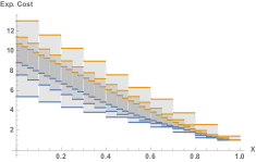
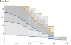
Figure 3: Upper (yellow) and lower (blue) expected cost functions of IMDPs $\mathcal{M}_{\mathcal{A}}(\Delta)$ for $\Delta\in\{0.1,0.05,0.025\}$ on $\mathcal{S}^{\prime}_{0}$ (left) and $\mathcal{S}^{\prime}_{0.7}$ (right).

Figure 3 shows the upper and lower expected costs that we obtain from the induced IMDPs. One can see how the intervals narrow with successive partition refinements. The bounds on the section $\mathcal{S}^{\prime}_{0}$ are closer and converge more uniformly than on $\mathcal{S}^{\prime}_{0.7}$. This shows that in the upper left region of the state space ($x<0.5,t\geq 0.7$) the adversary has a greater influence on the process than at the lower part of the state space ($x\sim 0$), and the difference between a cooperative and a non-cooperative adversary is more pronounced.

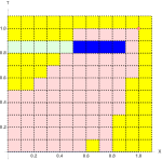
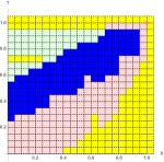
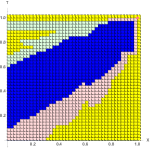
Figure 4: Strategies obtained from lower and upper expected cost approximations for $\mathcal{M}_{\mathcal{A}}(\Delta)$ for $\Delta=0.1,0.05,0.025$ (left to right).

Ultimately, induced strategies are of greater interest than the concrete cost functions. Once upper and lower expectations define the same strategy, further refinement may not be necessary. Figure 4 illustrates for the whole state space $\mathcal{S}$ the strategies $\sigma$ obtained from the lower (Equation (3)) and upper (Equation (4)) approximations. On regions colored blue and yellow, both strategies agree to take the fast and slow actions, respectively. The regions colored light green are those where the lower bound strategy chooses the fast action, and the upper bound strategy the slow action. Conversely for the regions colored light red. One can observe how the blue and yellow areas increase in size with successive partition refinements. However, this growth is not entirely monotonic: for example, some regions in the upper left that for $\Delta=0.1$ are yellow are sub-divided in successive refinements $\Delta=0.05,0.025$ into regions that are partly yellow, partly light green.

5.2 Analysis of learned strategies

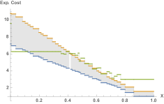
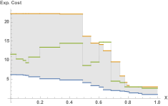
Figure 5: Expected cost functions along $S^{\prime}_{0}$ (left) and $S^{\prime}_{0.7}$ (right). Green: learned cost function; yellow/blue: upper/lower expected cost function obtained from IMDP.

We now turn to partitions computed by the reinforcement learning method developed in [9], and a comparison of the learned cost functions and strategies with those obtained from the induced IMDPs. We have implemented the semi-random walker in UPPAAL STRATEGO and used reinforcement learning to learn partitions, cost functions and strategies. Our learning framework produces a sequence of refinements, based on sampling $100$ additional runs for each refinement. In the following we consider the models learned after $k=27$ and $k=205$ refinements.

Figure 5 illustrates expected costs functions for the partition learned at $k=205$. One can observe a strong correlation between the bounds and the learned costs. Nevertheless, the learned cost function sometimes lies outside the given bounds. This is to be expected, since the random sampling process may produce data that is not sufficiently representative to estimate costs for some regions.

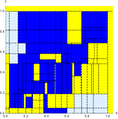
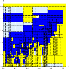
Figure 6: Comparison of the strategies obtained for the IMDP induced by the partition $\mathcal{A}(27)$ (left) and $\mathcal{A}(205)$ (right).

Turning again to the strategies obtained on the whole state space, we first note that the learned strategy at $k=205$, which is shown in Figure 1 (right) exhibits an overall similarity with the strategies illustrated in Figure 4, with the fast action preferred along a diagonal region in the middle of the state space. To understand the differences between the learning and IMDP results, it is important to note that in the learning setting $s_{0}=(0,0)$ is taken to be the initial state of interest, and all sampling starts there. As a result, regions that are unlikely to be reached (under any choice of actions) from this initial state will obtain very little relevant data, and therefore unreliable cost estimates. This is not necessarily a disadvantage, if we want to learn an optimal control strategy for processes starting at $s_{0}$. The value iteration process does not take into account the distinguished nature of $s_{0}$.

Figure 6 provides a detailed picture of the consistency of the strategies learned at $k=27$ and $k=205$ with the strategies obtained from value iteration over the same partitions. Drawn in blue/yellow are those regions where the learned strategy picks the fast/slow action, and at least one of upper or lower bound strategies selects the same action. Light blue are those regions where the learned strategy chooses the fast action, but both IMDP strategies select slow. In a single region in the $k=205$ partition (drawn in light yellow) the learned strategy chooses the slow, while both IMDP strategies select fast. As Figure 6 shows, the areas of greatest discrepancies (light blue) are those in the top left and bottom right, which are unlikely to be reached from initial state $(0,0)$.

6 Conclusion

In this paper we have developed theoretical foundations for the approximation of Euclidean MDPs by finite state space imprecise MDPs. We have shown that bounds on the cost function computed on the basis of the IMDP abstractions are correct, and that for bounded time horizons they converge to the exact costs when the IMDP abstractions are refined. We conjecture that this convergence also holds for the total cost of (potentially) infinite runs.

The results we here obtained provide theoretical underpinnings for the learning approach developed in [9]. Upper and lower bounds computed from induced IMDPs can be used to check the accuracy of learned value functions. As we have seen, data sparsity and sampling variance can make the learned cost functions fall outside computed bounds. One can also use value iteration on IMDP approximations directly as a tool for computing cost functions and strategies, which then would come with stronger guarantees than what we obtain through learning. However, compared to the learning approach, this has important limitations: first, we will usually only obtain a partial strategy that is uniquely defined only where upper and lower bounds lead to the same actions. Second, we will require a full model of the underlying EMDP, from which IMDP abstractions then can be derived, and the optimization problem over adversaries that is part of the value iteration process must be tractable. Reinforcement learning, on the other hand, can also be applied to black box systems, and its computational complexity is essentially independent of the complexities of the underlying dynamic system.

Appendix 0.A Total Variation Distance

The following lemma collects some basic facts about total variation distance:

Lemma 5

Let $\mathcal{A}$ be a finite set, and $P,P^{\prime}$ be distributions on $\mathcal{A}$ with $d_{\emph{tv}}(P,P^{\prime})\leq\epsilon$.

A

Let $f,f^{\prime}$ functions on $\mathcal{A}$ with values in $\mathbb{R}_{\geq 0}$ and $|f(\nu)-f^{\prime}(\nu)|\leq\epsilon$ for all $\nu$. Then

$$|\mathbb{E}[f]-\mathbb{E}^{\prime}[f^{\prime}]|\leq\epsilon\cdot(1+2\max_{\nu\in\mathcal{A}}f(\nu)),$$ (16)

where $\mathbb{E},\mathbb{E}^{\prime}$ denote expectation under $P$ and $P^{\prime}$, respectively.

B

For each $\nu\in\mathcal{A}$ let $Q_{\nu},Q_{\nu}^{\prime}$ be distributions on a space $\mathcal{S}$ (discrete or continuous), such that $d_{\emph{tv}}(Q_{\nu},Q_{\nu}^{\prime})\leq\epsilon$ for all $\nu$. Then

$$d_{\emph{tv}}(\sum_{\nu}P(\nu)Q_{\nu},\sum_{\nu}P^{\prime}(\nu)Q_{\nu}^{\prime})\leq 3\epsilon.$$ (17)

Proof

For A we write

$$|\mathbb{E}[f]-\mathbb{E}^{\prime}[f^{\prime}]|\leq|\mathbb{E}[f]-\mathbb{E}^{\prime}[f]|+|\mathbb{E}^{\prime}[f]-\mathbb{E}^{\prime}[f^{\prime}]|$$

With

$$|\mathbb{E}[f]-\mathbb{E}^{\prime}[f]|=|\sum_{\nu}P(\nu)f(\nu)-\sum_{\nu}P^{\prime}(\nu)f(\nu)|\leq\\ \sum_{\nu}f(\nu)|P(\nu)-P^{\prime}(\nu)|\leq\max_{\nu\in\mathcal{A}}f(\nu)2d_{\emph{tv}}(P,P^{\prime})$$

and

$$|\mathbb{E}^{\prime}[f]-\mathbb{E}^{\prime}[f^{\prime}]|\leq\epsilon$$

then (16) follows. The proof for B is very similar:

$$d_{\emph{tv}}\left(\sum_{\nu}P(\nu)Q_{\nu},\sum_{\nu}P^{\prime}(\nu)Q_{\nu}^{\prime}\right)\leq\\ d_{\emph{tv}}\left(\sum_{\nu}P(\nu)Q_{\nu},\sum_{\nu}P(\nu)Q_{\nu}^{\prime}\right)+d_{\emph{tv}}\left(\sum_{\nu}P(\nu)Q_{\nu}^{\prime},\sum_{\nu}P^{\prime}(\nu)Q_{\nu}^{\prime}\right).$$

Using the definition of total variation as $d_{\emph{tv}}(P,P^{\prime})=sup_{S\subseteq\mathcal{S}}|P(S)-P^{\prime}(S)|$ the first term on the right can be bounded by $\epsilon$, and the second by $2\epsilon$.

Appendix 0.B Proofs

See 1

Proof

For each $i$, $\pi\mapsto\mathcal{C}(\pi_{i})$ is $(\mathcal{B}^{K}\otimes 2^{\mathit{Act}})^{\infty}-{\mathcal{B}}_{+}$ measurable according to the measurability condition on $\mathcal{C}$. It follows that also $\mathcal{C}^{(N)}(\pi):=\sum_{i=1}^{N}\mathcal{C}(\pi_{i})$ is measurable for every $N$. Since $\mathcal{C}^{\infty}$ is the supremum of the $\mathcal{C}^{(N)}$, it is measurable [3, Proposition 2.1.4].

See 2

Proof

For fixed $(s,a)$, $T_{\sigma}$ is a probability measure on $\mathcal{B}^{K}\times 2^{\mathit{Act}}$ by construction. To show that for fixed $(B,A)$ the function $(s,a)\mapsto T_{\sigma}((s,a),(B,A))$ is measurable, we only need to consider the case of singletons $A=\{a^{\prime}\}$. By the measurability of $\sigma(\cdot)(a^{\prime})$ we can express $\sigma(\cdot)(a^{\prime})$ as the supremum of a monotone increasing sequence of simple measurable functions $\sigma^{(k)}(\cdot)(a^{\prime})$[1, Theorem 13.5]. For each $\sigma^{(k)}$ the integral $\int_{B}\sigma^{(k)}(s^{\prime})(\{a^{\prime}\})T(s,a,ds^{\prime})$ then decomposes into a weighted sum of integrals of the form $\int_{B\cap C_{i}}T(s,a,ds^{\prime})=T(s,a,B\cap C_{i})$, which are measurable in $s$ according to Definition 1. Finally,

$$\int_{B}\sup_{k}\sigma^{(k)}(s^{\prime})(\{a^{\prime}\})T(s,a,ds^{\prime})=\sup_{k}\int_{B}\sigma^{(k)}(s^{\prime})(\{a^{\prime}\})T(s,a,ds^{\prime})$$

by the monotone convergence theorem [1, Theorem 16.2], and measurability follows from the measurability of the supremum of measurable functions [1, Theorem 13.4].

See 3

Proof

By [1, Theorem 13.5] we can express $E$ as the supremum of a monotone increasing sequence of simple measurable functions $E^{(k)}$. For each $E^{(k)}$ the integral $\int_{t\in\mathcal{S}}E^{(k)}(t)\,T(s,a,\mathrm{d}t)$ then decomposes into a weighted sum of integrals of the form $\int_{t\in C_{i}}T(s,a,\mathrm{d}t)=T(s,a,C_{i})$, for some measurable set $C_{i}\subseteq\mathcal{S}$, which are measurable according to Definition 1. Since $E=\sup_{k}E^{(k)}$, by the monotone convergence theorem [1, Theorem 16.2],

$${\cal L}E(s) =\min_{a\in\mathit{Act}}\left(\mathcal{C}(s,a)+\sup_{k}\int_{t\in\mathcal{S}}E^{(k)}(t)\,T(s,a,\mathrm{d}t)\right)\,,$$

$${\cal L}^{\sigma}E(s) =\sum_{a\in\mathit{Act}}\sigma(s)(a)\cdot\left(\mathcal{C}(s,a)+\sup_{k}\int_{t\in\mathcal{S}}E^{(k)}(t)\,T(s,a,\mathrm{d}t)\right)\,,$$

From the above, measurability of ${\cal L}E$ follows from the measurability of $\mathcal{C}(\cdot,a)$, for all $a\in\mathit{Act}$, and of minima of measurable functions [1, Theorem 13.4]. Measurability of ${\cal L}^{\sigma}E$ follows similarly by additionally noticing that for any strategy $\sigma$, the $[0,1]$-valued function $\sigma(\cdot)(a)$ is measurable, for all $a\in\mathit{Act}$.

See 4

Proof

$\inf_{\sigma}{\cal L}^{\sigma}\leq{\cal L}$ follows by noticing that ${\cal L}=\inf_{d}{\cal L}^{d}$, where $d$ ranges only over deterministic strategies. To establish the reverse equality, notice that, for all $\sigma$ and $s\in\mathcal{S}$, $\sum_{a\in\mathit{Act}}\sigma(s)(a)=1$.

$${\cal L}E(s) =\sum_{a\in\mathit{Act}}\sigma(s)(a)\cdot{\cal L}E(s)$$

$$\leq\sum_{a\in\mathit{Act}}\sigma(s)(a)\cdot\left(\mathcal{C}(s,a)+\int_{t\in\mathcal{S}}E(t)\,T(s,a,\mathrm{d}t)\right)={\cal L}^{\sigma}(E)(s)\,.$$

Thus, ${\cal L}\leq{\cal L}^{\sigma}$, for all strategies $\sigma$. From this we obtain $\inf_{\sigma}{\cal L}^{\sigma}\geq{\cal L}$. ∎

See 1

Proof

We have to show that the following holds for all states $s\in\mathcal{S}$:

$$\mathbb{E}_{\sigma}(\mathcal{C},s)=\sum_{a\in\mathit{Act}}\sigma(s)(a)\cdot\left(\mathcal{C}(s,a)+\int_{t\in\mathcal{S}}\mathbb{E}_{\sigma}(\mathcal{C},t)\,T(s,a,\mathrm{d}t)\right)\,.$$ (18)

By monotone convergence theorem and linearity of the integral, we have

$$\mathbb{E}_{\sigma}(\mathcal{C},s) =\sup_{N}\int_{\pi\in\Pi}\sum_{i=1}^{N}\mathcal{C}(\pi_{i})\,P_{s,\sigma}(\mathrm{d}\pi)$$

$$=\int_{\pi\in\Pi}\mathcal{C}(\pi_{1})P_{s,\sigma}(\mathrm{d}\pi)+\sup_{N}\int_{\pi\in\Pi}\sum_{i=2}^{N}\mathcal{C}(\pi_{i})\,P_{s,\sigma}(\mathrm{d}\pi)$$

$$=\int_{\pi\in\Pi}\mathcal{C}(\pi_{1})P_{s,\sigma}(\mathrm{d}\pi)+\int_{\pi\in\Pi}\mathcal{C}^{\infty}(\pi_{>1})\,P_{s,\sigma}(\mathrm{d}\pi)\,.$$ (19)

By definition, the first expectation in (19) is just

$$\int_{\pi\in\Pi}\mathcal{C}(\pi_{1})\,P_{s,\sigma}(\mathrm{d}\pi) =\sum_{a\in\mathit{Act}}\mathcal{C}(s,a)\cdot\sigma(s)(a)\,.$$

and by a change of variable in the integral, the second expectation in (19) is

$$\int_{\pi\in\Pi}\mathcal{C}^{\infty}(\pi_{>1})\,P_{s,\sigma}(\mathrm{d}\pi) =\sum_{a\in\mathit{Act}}\sigma(s)(a)\cdot\int_{t\in\mathcal{S}}\left(\int_{\pi\in\Pi}\mathcal{C}^{\infty}(\pi)P_{t,\sigma}(\mathrm{d}\pi)\right)\,T(s,a,\mathrm{d}t)$$

$$=\sum_{a\in\mathit{Act}}\sigma(s)(a)\cdot\int_{t\in\mathcal{S}}\mathbb{E}_{\sigma}(\mathcal{C},t)\,T(s,a,\mathrm{d}t)\,.$$

Thus, (18) follows. ∎

See 2

Proof

By Lemma 4, Proposition 1 and monotonicity of ${\cal L}^{\sigma}$ we have

$$\mathbb{E}(\mathcal{C},\cdot)=\inf_{\sigma}\mathbb{E}_{\sigma}(\mathcal{C},\cdot)=\inf_{\sigma}{\cal L}^{\sigma}\mathbb{E}_{\sigma}(\mathcal{C},\cdot)\geq\inf_{\sigma}{\cal L}^{\sigma}\mathbb{E}(\mathcal{C},\cdot)={\cal L}\mathbb{E}(\mathcal{C},\cdot)\,.$$

Next we prove that if $E\geq{\cal L}E$, then $E\geq\mathbb{E}(\mathcal{C},\cdot)$. By induction on $n\geq 1$, we prove that, for all $s\in\mathcal{S}$ and strategies $\sigma$

$$({\cal L}^{\sigma})^{n}E(s)\geq\int_{\pi\in\Pi}\sum_{i=1}^{n}\mathcal{C}(\pi_{i})\,P_{s,\sigma}(\mathrm{d}\pi)\,.$$ (20)

The base case $n=1$ follows by definition of $P_{s,\sigma}(\mathrm{d}\pi)$ and because $E$ is positive:

$$\int_{\pi\in\Pi}\mathcal{C}(\pi_{1})\,P_{s,\sigma}(\mathrm{d}\pi) =\sum_{a\in\mathit{Act}}\mathcal{C}(s,a)\cdot\sigma(s)(a)$$

$$\leq\sum_{a\in\mathit{Act}}\sigma(s)(a)\cdot\left(\mathcal{C}(s,a)+\int_{t\in\mathcal{S}}E(t)\,T(s,a,\mathrm{d}t)\right)\,.$$

As for the inductive step, assume (20) holds for $n\geq 1$. Then

$$\int_{\pi\in\Pi}\sum_{i=1}^{n+1}\mathcal{C}(\pi_{i})\,P_{s,\sigma}(\mathrm{d}\pi)$$

$$=\int_{\pi\in\Pi}\mathcal{C}(\pi_{1})\,P_{s,\sigma}(\mathrm{d}\pi)+\int_{\pi\in\Pi}\sum_{i=2}^{n+1}\mathcal{C}(\pi_{i})\,P_{s,\sigma}(\mathrm{d}\pi)$$

$$=\sum_{a\in\mathit{Act}}\sigma(s)(a)\cdot\left(\mathcal{C}(s,a)+\int_{t\in\mathcal{S}}\left(\int_{\pi\in\Pi}\sum_{i=1}^{n}\mathcal{C}(\pi_{i})\,P_{t,\sigma}(\mathrm{d}\pi)\right)\,T(s,a,\mathrm{d}t)\right)$$

$$\leq\sum_{a\in\mathit{Act}}\sigma(s)(a)\cdot\left(\mathcal{C}(s,a)+\int_{t\in\mathcal{S}}({\cal L}^{\sigma})^{n}E(t)\,T(s,a,\mathrm{d}t)\right)$$

$$=({\cal L}^{\sigma})^{n+1}E(s)\,.$$

Let $d$ be the deterministic strategy such that ${\cal L}E={\cal L}^{d}E$. By hypothesis, $E\geq{\cal L}E$, and by monotonicity of ${\cal L}^{d}$, we obtain $E\geq({\cal L}^{d})^{n}E$, for all $n\geq 1$. Thus, by (20) and monotone convergence theorem, for all $s\in\mathcal{S}$

$$E(s)\geq\sup_{n\geq 1}({\cal L}^{d})^{n}E(s)\geq\sup_{n\geq 1}\int_{\pi\in\Pi}\sum_{i=1}^{n}\mathcal{C}(\pi_{i})\,P_{s,d}(\mathrm{d}\pi)=\mathbb{E}_{d}(\mathcal{C},s)\,.$$

Since $\mathbb{E}(\mathcal{C},s)=\inf_{\sigma}\mathbb{E}_{\sigma}(\mathcal{C},s)$, from the above we have $E(s)\geq\mathbb{E}(\mathcal{C},s)$. ∎

See 2.1

Proof

The chain $\bot\leq L^{1}\leq L^{2}\leq\dots$ is monotonically increasing. This is immediate from $\bot\leq{\cal L}\bot$ and monotonicity of the operator ${\cal L}$.

Next we show that $L$ is a fixed point of the ${\cal L}$ operator. Clearly, $\bot\leq{\cal L}L$, and by monotonicity of ${\cal L}$, for all $n\geq 1$, $L^{n}\leq{\cal L}L$. Hence $L\leq{\cal L}L$. Now we establish ${\cal L}L\leq L$. If $L(s)=\infty$, the inequality holds trivially on $s$. Assume $L(s)<\infty$. Then there exist a sequence $(a_{n})_{n\geq 0}\in\mathit{Act}$ such that

$$L(s) =\sup_{n\geq 0}\min_{a\in\mathit{Act}}\left(\mathcal{C}(s,a)+\int_{t\in\mathcal{S}}L^{n}(t)\,T(s,a,\mathrm{d}t)\right)$$

$$=\sup_{n\geq 0}\left(\mathcal{C}(s,a_{n})+\int_{t\in\mathcal{S}}L^{n}(t)\,T(s,a_{n},\mathrm{d}t)\right)\,.$$

Let $\mathcal{S}^{\infty}=\{t\in\mathcal{S}\mid L(t)=\infty\}$. In the following we show that

$$\exists N\geq 0\text{ such that, }\forall n\geq N.\,T(s,a_{n},\mathcal{S}^{\infty})=0\,.$$ (21)

If $S^{\infty}=\emptyset$, (21) holds trivially. Let $S^{\infty}\neq\emptyset$. Assume by contradiction that for all $N\geq 0$ there exists $n\geq N$ such that $T(s,a_{n},\mathcal{S}^{\infty})>0$. This is equivalent to the existence of a subsequence $(a_{k})$ such that for all $a_{k}$, $T(s,a_{k},\mathcal{S}^{\infty})>0$. For $b\in\mathbb{R}$ and $n\geq 0$, denote by $E_{b}^{n}$ the set $\{t\in\mathcal{S}\mid L^{n}(t)\geq b\}$. Then,

$$\mathcal{S}^{\infty}=\{t\in\mathcal{S}\mid\forall b\in\mathbb{R}.\,\exists n\geq 0.\,L^{n}(t)\geq b\}=\bigcap_{b\in\mathbb{R}}\bigcup_{n\geq 0}E_{b}^{n}\,.$$

Moreover, for all $b,b^{\prime}\in\mathbb{R}$ and $n\geq 0$, if $b\geq b^{\prime}$ then $E_{b}^{n}\subseteq E_{b^{\prime}}^{n}$ and by monotonicity of the operator ${\cal L}$, $E_{b}^{n}\subseteq E_{b}^{n+1}$. Thus, by [1, Theorem 10.2], for all $a_{k}$ and $b\in\mathbb{R}$

$$T(s,a_{k},\mathcal{S}^{\infty})=\inf_{b\in\mathbb{R}}T(s,a_{k},\bigcup_{n\geq 0}E_{b}^{n})\,,$$ (22)

$$T(s,a_{k},\bigcup_{n\geq 0}E_{b}^{n})=\sup_{n\geq 0}T(s,a_{k},E_{b}^{n})\,.$$ (23)

Since $T(s,a_{k},\mathcal{S}^{\infty})>0$, by (22), , for all $a_{k}$, $T(s,a_{k},\bigcup_{n\geq 0}E_{b}^{n})>0$. Consequently, by (23), for all $b\in\mathbb{R}$, exist $k^{\prime}$ such that $T(s,a_{k^{\prime}},E_{b}^{k^{\prime}})\geq 0$. Thus, by

$$L(s)\geq\int_{t\in E_{b}^{k^{\prime}}}L^{k^{\prime}}(t)\,T(s,a_{k^{\prime}},\mathrm{d}t)\geq\int_{t\in E_{b}^{k^{\prime}}}b\,T(s,a_{k^{\prime}},\mathrm{d}t)=b\cdot T(s,a_{k^{\prime}},E_{b}^{k^{\prime}})$$

and the fact that $b$ can assume arbitrarily large values, $L(s)=\infty$. This contradicts our initial assumption that $L(s)<\infty$. Therefore (21) must hold.

By (21), for all $n\geq N$, $\int_{t\in\mathcal{S}}L^{n}(t)\,T(s,a_{n},\mathrm{d}t)=\int_{t\in\mathcal{S}}(L(t)-L(t))L^{n}(t)\,T(s,a_{n},\mathrm{d}t)$. Thus the following hold:

$$L(s) =\sup_{n\geq N}\left(\mathcal{C}(s,a_{n})+\int_{t\in\mathcal{S}}L^{n}(t)\,T(s,a_{n},\mathrm{d}t)\right)$$

$$=\sup_{n\geq N}\left(\mathcal{C}(s,a_{n})+\int_{t\in\mathcal{S}}L(t)\,T(s,a_{n},\mathrm{d}t)\right)+\Delta(s)$$

$$\geq\sup_{n\geq N}\min_{a\in\mathit{Act}}\left(\mathcal{C}(s,a)+\int_{t\in\mathcal{S}}L(t)\,T(s,a,\mathrm{d}t)\right)+\Delta(s)$$

$$={\cal L}L(s)+\Delta(s)\,,$$

where

$$\Delta(s)=\sup_{n\geq N}\int_{t\in\mathcal{S}}\Big{(}L^{n}(t)-L(t)\Big{)}\,T(s,a_{n},\mathrm{d}t)\,.$$

Hence, if $\Delta(s)=0$, we get $L(s)\geq{\cal L}L(s)$.

The finiteness of $\mathit{Act}$ ensures the existence of an action $a^{\prime}\in\mathit{Act}$ repeating infinitely often in $(a_{n})_{n\geq N}$. Thus exists a subsequence $(n_{k})$ such that, for all $n_{k}$

$$\int_{t\in\mathcal{S}}\Big{(}L^{n_{k}}(t)-L(t)\Big{)}\,T(s,a_{n_{k}},\mathrm{d}t)=\int_{t\in\mathcal{S}}\Big{(}L^{n_{k}}(t)-L(t)\Big{)}\,T(s,a^{\prime},\mathrm{d}t)\,.$$

Therefore

$$\Delta(s)=\sup_{n\in(n_{k})}\int_{t\in\mathcal{S}}\Big{(}L^{n}(t)-L(t)\Big{)}\,T(s,a^{\prime},\mathrm{d}t)\,,$$

and, by monotone convergence theorem, $\Delta(s)=0$.

Finally, we show that $L=\mathbb{E}(\mathcal{C},\cdot)$. By monotonicity of ${\cal L}$, for all $n\geq 0$, we have $L^{n}\leq\mathbb{E}(\mathcal{C},\cdot)$. Hence $L\leq\mathbb{E}(\mathcal{C},\cdot)$. The reverse inequality $L\geq\mathbb{E}(\mathcal{C},\cdot)$ follows by Proposition 2 since $L\geq{\cal L}L$. ∎

See 3.1

Proof

Step 1: The sequence $L^{\operatorname*{opt},k}$ is monotonically increasing: this is immediate from the facts that $L^{\operatorname*{opt},1}\geq\bot$ because $\mathcal{C}^{\operatorname*{opt}}\geq 0$, and $C\geq C^{\prime}\Rightarrow{\cal L}^{\operatorname*{opt}}C\geq{\cal L}^{\operatorname*{opt}}C^{\prime}$.

Step 2: We show that $L^{\operatorname*{opt}}$ is a fixed point of the ${\cal L}$ operator. Let

$$\mathcal{S}^{\operatorname*{opt},\infty}:=\{s\in\mathcal{S}:L^{\operatorname*{opt}}(s)=\infty\}\ \ \mbox{and}\ \ \mathcal{S}^{\operatorname*{opt},<\infty}:=\mathcal{S}\setminus\mathcal{S}^{\operatorname*{opt},\infty}.$$

By monotonicity, for $s\in\mathcal{S}^{\operatorname*{opt},\infty}$ we have ${\cal L}^{\operatorname*{opt}}L^{\operatorname*{opt}}(s)=\infty$. Now let $s\in\mathcal{S}^{\operatorname*{opt},<\infty}$. We define separately for the two cases of $\operatorname*{opt}$:

$$\begin{array}[]{lll}\mathit{Act}^{\min,<\infty}(s)&:=&\{a\in\mathit{Act}|\exists T\in T^{*}(s,a)\ \mbox{s.t.}\ T(\mathcal{S}^{\min,\infty})=0\},\\ \mathit{Act}^{\max,<\infty}(s)&:=&\{a\in\mathit{Act}|\forall T\in T^{*}(s,a):\ T(\mathcal{S}^{\max,\infty})=0\}.\end{array}$$

The set $\mathit{Act}^{\operatorname*{opt},<\infty}(s)$ is non-empty (the closedness of $T^{*}$ is again required here), and we can limit the optimization to actions that after the adversary’s choice do not lead to infinite cost states:

$${\cal L}^{\operatorname*{opt}}L^{\operatorname*{opt}}(s)=\\ \min_{a\in\mathit{Act}^{\operatorname*{opt},<\infty}(s)}\left(\mathcal{C}^{\operatorname*{opt}}(s,a)+\operatorname*{opt}_{T\in T^{*}(s,a)}\sum_{s^{\prime}\in\mathcal{S}^{\operatorname*{opt},<\infty}}T(s^{\prime})L^{\operatorname*{opt}}(s^{\prime})\right).$$ (24)

Moreover, the restriction of the minimization to actions from $\mathit{Act}^{\operatorname*{opt},<\infty}$ also already is valid for the definition of ${\cal L}^{\operatorname*{opt}}L^{\operatorname*{opt},n}(s)$ for all sufficiently large $n$. We have that $L^{\operatorname*{opt},n}\rightarrow L^{\operatorname*{opt}}$ uniformly on the (finite) set $\mathcal{S}^{\operatorname*{opt},<\infty}$. It follows that for all $s\in\mathcal{S}^{\operatorname*{opt},<\infty}$ and $a\in\mathit{Act}^{\operatorname*{opt},<\infty}$:

$$\operatorname*{opt}_{T\in T^{*}(s,a)}\sum_{s^{\prime}\in\mathcal{S}^{\operatorname*{opt},<\infty}}T(s^{\prime})L^{\operatorname*{opt}}(s^{\prime})=\\ \lim_{n\rightarrow\infty}\operatorname*{opt}_{T\in T^{*}(s,a)}\sum_{s^{\prime}\in\mathcal{S}^{\operatorname*{opt},<\infty}}T(s^{\prime})L^{\operatorname*{opt},n}(s^{\prime}).$$ (25)

With (24) it then follows that

$${\cal L}^{\operatorname*{opt}}L^{\operatorname*{opt}}(s)=\lim_{n\rightarrow\infty}{\cal L}^{\operatorname*{opt}}L^{\operatorname*{opt},n}(s)=L^{\operatorname*{opt}}(s).$$

Step 3: $\mathbb{E}^{\operatorname*{opt}}$ is the least fixed-point of the ${\cal L}^{\operatorname*{opt}}$-operator. That $\mathbb{E}^{\operatorname*{opt}}$ is a fixed-point follows immediately from our restriction to stationary and memoryless strategies.

Let $C\geq 0$ be an arbitrary fixed-point of ${\cal L}^{\operatorname*{opt}}$. Recalling (7), we can then write

$$C(s)=\operatorname*{opt}_{\alpha_{T}}\left(\mathcal{C}^{\operatorname*{opt}}(s,\sigma^{\operatorname*{opt}}(C)(s))+\sum_{s^{\prime}}\alpha_{T}(s,\sigma^{\operatorname*{opt}}(C))(s^{\prime})C(s^{\prime})\right).$$ (26)

Un-rolling this recurrence for $n$ steps gives

$$C(s)=\operatorname*{opt}_{\alpha_{T}}\left(\sum_{k=1}^{n}\mathbb{E}^{(k)}_{s,\sigma^{\operatorname*{opt}}(C),\alpha_{T}}(\mathcal{C}^{\operatorname*{opt}}(s_{k},\sigma^{\operatorname*{opt}}(C)(s_{k})))+\mathbb{E}^{(n+1)}_{s,\sigma^{\operatorname*{opt}}(C),\alpha_{T}}(C)\right),$$ (27)

where $\mathbb{E}^{(k)}_{s,\sigma^{\operatorname*{opt}}(C),\alpha^{\operatorname*{opt}}_{T}(C)}$ is the expectation over the state distribution at step $k$ defined by $\sigma^{\operatorname*{opt}}(C)$, $\alpha^{\operatorname*{opt}}_{T}(C)$ and initial state $s$. Since $C$ is non-negative, we can lower-bound (27) by dropping the expectation $\mathbb{E}^{(n+1)}_{s,\sigma^{\operatorname*{opt}}(C),\alpha_{T}}(C)$. Then taking the limit $n\rightarrow\infty$ gives

$$C(s)\geq\operatorname*{opt}_{\alpha_{T}}\lim_{n\rightarrow\infty}\left(\sum_{k=1}^{n}\mathbb{E}^{(k)}_{s,\sigma^{\operatorname*{opt}}(C),\alpha_{T}}(\mathcal{C}^{\operatorname*{opt}}(s_{k},\sigma^{\operatorname*{opt}}(C)(s_{k})))\right)\\ \geq\min_{\sigma}\operatorname*{opt}_{\alpha_{T}}\lim_{n\rightarrow\infty}\left(\sum_{k=1}^{n}\mathbb{E}^{(k)}_{s,\sigma,\alpha_{T}}(\mathcal{C}^{\operatorname*{opt}}(s_{k},\sigma(s_{k})))\right)\\ =\mathbb{E}^{\operatorname*{opt}}(\mathcal{C}^{\operatorname*{opt}}(\pi),s),$$

where $\sigma^{\operatorname*{opt}}$ in the second line now is the strategy that actually achieves the minimum in (3), respectively (4).

Step 4: Putting things together: From the monotony of the ${\cal L}^{\operatorname*{opt}}$ operator and the fixed point property of $\mathbb{E}^{\operatorname*{opt}}$ it follows that $\mathbb{E}^{\operatorname*{opt}}\geq L^{\operatorname*{opt}}$. From the fixed point property of $L^{\operatorname*{opt}}$ and the minimality property of $\mathbb{E}^{\operatorname*{opt}}$ it follows that $\mathbb{E}^{\operatorname*{opt}}\leq L^{\operatorname*{opt}}$.

See 4.1

Proof

We first consider the inequality $\mathbb{E}_{\mathcal{M}_{\mathcal{A}}}^{\min}(\mathcal{C}_{\mathcal{A}}^{*},[s]_{\mathcal{A}})\leq\mathbb{E}_{\mathcal{M}}(\mathcal{C},s)$. Let $L^{\min,k}_{\mathcal{M}_{\mathcal{A}}}$ denote the cost function obtained after the $k$’th round of value iteration in $\mathcal{M}_{\mathcal{A}}$, and $L^{k}_{\mathcal{M}}$ denote the cost function after the $k$’th round of value iteration in $\mathcal{M}$. By induction we show that $L^{\min,k}_{\mathcal{M}_{\mathcal{A}}}(\nu)\leq L^{k}_{\mathcal{M}}(s)$ for all $k\geq 0$ and all $\nu,s$ with $s\in\nu$. For $k=0$ this is true according to the initialization. For $k+1$ we can then write:

$$L^{\min,k+1}_{\mathcal{M}_{\mathcal{A}}}(\nu)=\min_{a\in\mathit{Act}}\min_{s\in\nu}\left(\mathcal{C}^{\min}(\nu,a)+\sum_{\nu^{\prime}}T_{\mathcal{A}}(s,a)(\nu^{\prime})L^{\min,k}_{\mathcal{M}_{\mathcal{A}}}(\nu^{\prime})\right)\\ =\min_{s\in\nu}\min_{a\in\mathit{Act}}\left(\mathcal{C}^{\min}(\nu,a)+\sum_{\nu^{\prime}}\int_{\nu^{\prime}}T(s,a)(t)L^{\min,k}_{\mathcal{M}_{\mathcal{A}}}(\nu^{\prime})dt\right)\\ \leq\min_{s\in\nu}\min_{a\in\mathit{Act}}\left(\mathcal{C}(s,a)+\sum_{\nu^{\prime}}\int_{\nu^{\prime}}T(s,a)(t)L^{k}_{\mathcal{M}}(t)dt\right)=\min_{s\in\nu}L^{k+1}_{\mathcal{M}}(s)$$ (28)

The inequality $\mathbb{E}_{\mathcal{M}}(\mathcal{C},s)\leq\mathbb{E}_{\mathcal{M}_{\mathcal{A}}}^{\max}(\mathcal{C}_{\mathcal{A}}^{*},[s]_{\mathcal{A}})$ is proven in the same way, here noting that $\min_{a}\max_{s}\geq\max_{s}\min_{a}$. The same line of argument can also be used to establish the inequalities (11),(12). ∎

See 4.2

Proof

By induction on $N$. For $N=1$ let $\delta$ be such that for all $\mathcal{A}$ with $\delta(\mathcal{A})\leq\delta$ it holds that for all $\nu\in\mathcal{A}$: $\mathcal{C}^{\max}(\nu,a)-\mathcal{C}^{\min}(\nu,a)\leq\epsilon$, and $d_{\emph{tv}}(T(s,a),T(s^{\prime},a))\leq\epsilon$ for all $s,s^{\prime}\in\nu$. Then (13) holds because

$$|\mathbb{E}^{N}_{\tau,\alpha^{+}}-\mathbb{E}^{N}_{\tau,\alpha^{-}}|\leq\mathcal{C}^{\max}(\nu_{1},\tau(\nu_{1}))-\mathcal{C}^{\min}(\nu_{1},\tau(\nu_{1})),$$

and (14) follows from

$$P^{1}_{\tau,\alpha^{+[-]}}=\alpha_{T}^{+[-]}(\nu_{1},\tau(\nu_{1})).$$

For the induction step, let $c^{\max}:=\max_{s\in\mathcal{S},a\in\mathit{Act}}C(s,a)<\infty$. Let $\delta$ be such that (13) and (14) hold for $N-1$ and $\epsilon^{\prime}:=\min\{\epsilon/(2(1+2c^{\max})),\epsilon/3\}$, and also such that for all $\nu$ with $\delta(\nu)\leq\delta$ and all $a\in\mathit{Act}$: $\mathcal{C}^{\max}(\nu,a)-\mathcal{C}^{\min}(\nu,a)\leq\epsilon^{\prime}$, and $d_{\emph{tv}}(T(s,a),T(s^{\prime},a))\leq\epsilon^{\prime}$ for all $s,s^{\prime}\in\nu$. Let $\mathcal{A}$ have granularity $\leq\delta$. We then have

$$|\mathbb{E}^{N}_{\tau,\alpha^{+}}-\mathbb{E}^{N}_{\tau,\alpha^{-}}|=\\ |\mathbb{E}^{N-1}_{\tau,\alpha^{+}}+\sum_{\nu\in\mathcal{A}}P^{N-1}_{\tau,\alpha^{+}}(\nu)\alpha_{C}^{+}(\nu,\tau(\nu))-(\mathbb{E}^{N-1}_{\tau,\alpha^{-}}+\sum_{\nu\in\mathcal{A}}P^{N-1}_{\tau,\alpha^{-}}(\nu)\alpha_{C}^{-}(\nu,\tau(\nu)))|\leq\\ |\mathbb{E}^{N-1}_{\tau,\alpha^{+}}-\mathbb{E}^{N-1}_{\tau,\alpha^{-}}|+|\sum_{\nu\in\mathcal{A}}P^{N-1}_{\tau,\alpha^{+}}(\nu)\alpha_{C}^{+}(\nu,\tau(\nu))-\sum_{\nu\in\mathcal{A}}P^{N-1}_{\tau,\alpha^{-}}(\nu)\alpha_{C}^{-}(\nu,\tau(\nu)))|$$

By induction hypothesis, the left term is bounded by $\epsilon^{\prime}<\epsilon/2$. According to Lemma 5 A, the right term is bounded by $\epsilon/2$, thus yielding (13).

The bound (14) directly follows from Lemma 5 B. ∎

References

• Billingsley [1986] P. Billingsley. Probability and Measure. John Wiley, second edition edition, 1986.
• Chen et al. [2013] T. Chen, T. Han, and M. Kwiatkowska. On the complexity of model checking interval-valued discrete time markov chains. Information Processing Letters, 113(7):210–216, 2013.
• Cohn [1980] D. L. Cohn. Measure Theory. Birkhäuser, 1980.
• Crossman et al. [2009] R. Crossman, P. Coolen-Schrijner, D. Škulj, and F. Coolen. Imprecise markov chains with an absorbing state. In Proceedings of the Sixth International Symposium on Imprecise Probability: Theories and Applications (ISIPTA), pages 119–128. Citeseer, 2009.
• David et al. [2015] A. David, P. G. Jensen, K. G. Larsen, M. Mikučionis, and J. H. Taankvist. Uppaal Stratego. In TACAS 2015, pages 206–211. Springer, 2015.
• Derisavi et al. [2003] S. Derisavi, H. Hermanns, and W. H. Sanders. Optimal state-space lumping in markov chains. Information Processing Letters, 87(6):309–315, 2003.
• Erreygers and De Bock [2018] A. Erreygers and J. De Bock. Computing inferences for large-scale continuous-time markov chains by combining lumping with imprecision. In International Conference Series on Soft Methods in Probability and Statistics, pages 78–86. Springer, 2018.
• Itoh and Nakamura [2007] H. Itoh and K. Nakamura. Partially observable markov decision processes with imprecise parameters. Artificial Intelligence, 171(8-9):453–490, 2007.
• Jaeger et al. [2019] M. Jaeger, P. G. Jensen, K. G. Larsen, A. Legay, S. Sedwards, and J. H. Taankvist. Teaching stratego to play ball: Optimal synthesis for continuous space mdps. In International Symposium on Automated Technology for Verification and Analysis, pages 81–97. Springer, 2019.
• Kwiatkowska et al. [2006] M. Z. Kwiatkowska, G. Norman, and D. Parker. Game-based abstraction for markov decision processes. In (QEST 2006), pages 157–166. IEEE Computer Society, 2006. ISBN 0-7695-2665-9. doi: 10.1109/QEST.2006.19.
• Lun et al. [2018] Y. Z. Lun, J. Wheatley, A. D’Innocenzo, and A. Abate. Approximate abstractions of markov chains with interval decision processes. In A. Abate, A. Girard, and M. Heemels, editors, ADHS 2018, volume 51 of IFAC-PapersOnLine, pages 91–96. Elsevier, 2018. doi: 10.1016/j.ifacol.2018.08.016.
• Puterman [2005] M. L. Puterman. Markov Decision Processes. Wiley, 2005.
• Rubino and Sericola [1991] G. Rubino and B. Sericola. A finite characterization of weak lumpable markov processes. part i: The discrete time case. Stochastic processes and their applications, 38(2):195–204, 1991.
• Troffaes et al. [2015] M. Troffaes, J. Gledhill, D. Škulj, and S. Blake. Using imprecise continuous time markov chains for assessing the reliability of power networks with common cause failure and non-immediate repair. SIPTA, 2015.
• White III and Eldeib [1994] C. C. White III and H. K. Eldeib. Markov decision processes with imprecise transition probabilities. Operations Research, 42(4):739–749, 1994.