Clustering and Halo Abundances in Early Dark Energy Cosmological Models

Abstract

$\Lambda$CDM cosmological models with Early Dark Energy (EDE) have been proposed to resolve tensions between the Hubble constant $H_{0}=100h$ km s^-1 Mpc^-1 measured locally, giving $h\approx 0.73$, and $H_{0}$ deduced from Planck cosmic microwave background (CMB) and other early universe measurements plus $\Lambda$CDM, giving $h\approx 0.67$. EDE models do this by adding a scalar field that temporarily adds dark energy equal to about 10% of the cosmological energy density at the end of the radiation-dominated era at redshift $z\sim 3500$. Here we compare linear and nonlinear predictions of a Planck-normalized $\Lambda$CDM model including EDE giving $h=0.728$ with those of standard Planck-normalized $\Lambda$CDM with $h=0.678$. We find that nonlinear evolution reduces the differences between power spectra of fluctuations at low redshifts. As a result, at $z=0$ the halo mass functions on galactic scales are nearly the same, with differences only 1-2%. However, the differences dramatically increase at high redshifts. The EDE model predicts 50% more massive clusters at $z=1$ and twice more galaxy-mass halos at $z=4$. Even greater increases in abundances of galaxy-mass halos at higher redshifts may make it easier to reionize the universe with EDE. Predicted galaxy abundances and clustering will soon be tested by JWST observations. Positions of baryonic acoustic oscillations (BAOs) and correlation functions differ by about 2% between the models – an effect that is not washed out by nonlinearities. Both standard $\Lambda$CDM and the EDE model studied here agree well with presently available acoustic-scale observations, but DESI and Euclid measurements will provide stringent new tests.

1 Introduction

Combined late-universe measurements give the value of the Hubble constant $h=0.733\pm 0.008$ according to a recent review of Verde et al. (2019). This value of the expansion rate is in as much as $6\sigma$ conflict with the value $h=0.674\pm 0.005$ from the Planck measurements of the cosmic background radiation (CMB) temperature and polarization and other early-universe observations extrapolated to the present epoch using standard $\Lambda$CDM (Planck Collaboration et al., 2018). This discrepancy is unlikely to be a statistical fluke, and it is not easily attributable to any systematic errors (e.g., Freedman, 2017; Riess et al., 2019a; Aylor et al., 2019). Instead, it may be telling us that there is a missing ingredient in standard $\Lambda$CDM. Of the many potential explanations that have been proposed, a brief episode of early dark energy (EDE) around the time of matter dominance followed by $\Lambda$CDM evolution (Poulin et al., 2019; Knox & Millea, 2020; Smith et al., 2020; Agrawal et al., 2019; Lin et al., 2019) has received perhaps the most attention. For the model we consider here, Poulin et al. (2019) and Smith et al. (2020, SPA20) have shown that their fluctuating scalar field EDE model can fit all the CMB data as well as the usual standard 6-parameter $\Lambda$CDM does, and also give $H_{0}$ in agreement with the recent local-universe measurements. As Figure 1 shows, in this model the early dark energy contributes a maximum of only about 10% to the total cosmic density at redshifts $z\sim 3500$, at the end of the era of radiation domination and the beginning of matter domination.

The resulting best-fit cosmic parameters (see Table 1) are interestingly different from those of standard $\Lambda$CDM. In particular, both the primordial power spectrum amplitude $A_{s}$ and $\sigma_{8}$, measuring the linear amplitude today at $8\mbox{$h^{-1}$Mpc}$, are larger than for the latest Planck analysis with standard $\Lambda$CDM. Also, $n_{s}$, the slope of the power primordial power spectrum is larger than for standard $\Lambda$CDM. And with the higher $H_{0}$, the present age of the universe is 13.0 Gyr rather than 13.8 Gyr. Such modifications of the cosmological parameters are also produced in other recent papers on EDE (Agrawal et al., 2019; Lin et al., 2019).

Particle theory provides many scalar fields that could have nonzero potential energy temporarily preserved by Hubble friction, leading to temporary episodes of effective dark energy (e.g., Dodelson et al., 2000; Griest, 2002; Kamionkowski et al., 2014). It has long been known that dark energy contributions at early cosmic times can imply modifications of CMB, big-bang nucleosynthesis, and large-scale structure formation (Doran et al., 2001; Müller et al., 2004; Bartelmann et al., 2006).

Only recently has resolving the Hubble tension become a motivation for EDE (Karwal & Kamionkowski, 2016; Poulin et al., 2019). The challenge lies in finding ways in which the Hubble parameter inferred from the CMB can be made larger without introducing new tensions with the detailed CMB peak structure and/or other well established cosmological constraints. In particular, all solutions are constrained by the remarkable precision (roughly one part in $10^{4}$) with which the angular scale $\theta_{a}$ of the acoustic peaks in the CMB power spectrum is fixed. Roughly speaking, this angular scale is set by $\theta_{a}\propto r_{s}/D_{A}$, where $r_{s}$ is the comoving sound horizon at the surface of last scatter and $D_{A}$ is the comoving distance to the surface of last scatter.

There are two possibilities to keep $\theta_{a}$ fixed: keep $D_{A}$ fixed by compensating the increase of energy today ($H_{0}$ higher means higher energy density today) by decreasing the energy density at earlier times through a change to the late-time expansion history, or decreasing $r_{s}$ by the same amount as $D_{A}$ through a change to the early-time physics. However, modifications to the late-time expansion history are constrained by measurements of baryonic acoustic oscillations and luminosity distance to supernovae, and early-time solutions are constrained by the detailed structure of the higher acoustic peaks in the CMB power spectra (Bernal et al., 2016). Even so, Poulin et al. (2018) and subsequent studies (Poulin et al., 2019; Agrawal et al., 2019; Smith et al., 2020; Lin et al., 2019) were able to find regions of the parameter space of EDE models that provide a good fit to the data. Still, more work must be done — both in terms of theory and new measurements — to assess the nature of viable EDE models.

We have chosen to focus on the Smith et al. (2020) version of EDE because it was engineered to fit the details of the high-$l$ CMB polarization data, and because it represents the best fit to the local $H_{0}$ measurements and the largest deviation of the cosmological parameters from standard $\Lambda$CDM, which should lead to the clearest differences in testable predictions. These new cosmological models will make specific predictions for galaxy mass and luminosity functions and galaxy clustering. Given that these phenomena arise from nonlinear evolution of primordial perturbations and involve gas dynamics, the power of numerical simulations is essential. Of course, it is possible that the result of such observational tests of EDE will be to eliminate this class of cosmological models. But if not, EDE potentially tells us about a phenomenon that contributes to early cosmic evolution, and about another scalar field important in the early universe besides the putative inflaton responsible for the cosmic inflation that set the stage for the Big Bang.

There were some earlier efforts to study effects of nonlinear evolution in models called early dark energy (Bartelmann et al., 2006; Grossi & Springel, 2009; Fontanot et al., 2012; Francis et al., 2009). However, models for the dark energy used in those papers are very different as compared with those discussed in this paper. As a matter of fact, there is little in common – with the exception of the name EDE – between those models and the model we consider here. The equation of state $w$ of dark energy $P=w\rho c^{2}$ in those papers is $w=-1$ only at $z=0$ and has significant deviations from $w=-1$ at low redshifts. For example, models used by Grossi & Springel (2009) and Fontanot et al. (2012) had $w=-0.7$ at $z=1$ and $w=-0.4$ at $z=5$. This should be compared with $w=-1$ at $z\lesssim 1000$ in our EDE model.

In the sense of dynamics of growth of fluctuations in the matter-dominated era in our EDE model, we are dealing with a vanilla $\Lambda$CDM model with the only modification being the spectrum of fluctuations. Even the spectrum of fluctuations is not much different: a 2% change in $\sigma_{8}$ and 0.02 difference in the slope of the spectrum. With these small deviations, one might imagine that the final non-linear statistics (such as power, correlation functions, halo mass functions) would be very similar. But instead we find very significant differences, especially at redshifts $z>1$.

The $S_{8}$ tension is the conflict between weak lensing and other local observations that imply a relatively low value of $S_{8}\equiv\sigma_{8}\sqrt{\Omega_{m}/0.3}$ and the higher value of $S_{8}$ of both the Planck-normalized $\Lambda$CDM and the EDE model considered here (Smith et al., 2020). Our EDE model has $\sigma_{8}=0.836$, larger than $\sigma_{8}=0.820$ of our fiducial Planck 2013 MultiDark model or the Planck 2018 value $\sigma_{8}=0.811\pm 0.006$. But what is determined by CMB observations is $\Omega_{m}h^{2}$, and the higher value of $H_{0}$ with EDE means that the resulting $S_{8}=0.830$ is identical to that from Planck 2018 (Combined value, Table 1 of Planck Collaboration et al., 2018).

The latest weak lensing measurements of $S_{8}$ are the Dark Energy Survey year 1 (DES-Y1) cosmic shear results $S_{8}=0.782^{+0.027}_{-0.027}$ (Troxel et al., 2018); the Hyper Suprime-Cam Year 1 (HSC-Y1) cosmic shear power spectra, giving $S_{8}=0.800^{+0.029}_{-0.028}$ (Hikage et al., 2019); and the HSC-Y1 cosmic shear two-point correlation functions, giving $S_{8}=0.804^{+0.032}_{-0.029}$ (Hamana et al., 2020). These measurements are all in less than $2\sigma$ disagreement with $S_{8}=0.830$ from Planck-normalized $\Lambda$CDM and our EDE model.

Hill et al. (2020) claims that the EDE model considered here, and other EDE models, are in serious tension with large scale structure measurements. They cite the DES-Y1 result $S_{8}=0.773^{+0.026}_{-0.020}$, obtained by combining weak lensing with galaxy clustering (Abbott et al., 2019), which disagrees by $2.3\sigma$ with $S_{8}=0.830$. However, Abbott et al. (2019) allowed the total neutrino mass free to vary, which leads to a somewhat lower DES-inferred $S_{8}$ than that, $S_{8}=0.792\pm 0.024$, which arises if $\sum m_{\nu}=0.06$ eV is fixed, as the Planck team (Planck Collaboration et al., 2018) and we have done. Similarly, the shear only result was analyzed by the SPTPol collaboration with the same convention as ours; they obtained $S_{8}=0.79^{+0.4}_{-0.029}$ (Bianchini et al., 2020), to be compared with $S_{8}=0.782\pm 0.027$ once the sum of neutrino masses is left free to vary (Troxel et al., 2018). While there is indeed some $S_{8}$ tension between the DES-Y1 measurements and the prediction of our EDE model, it remains true that the addition of a brief period of early dark energy resolves the $\Lambda$CDM Hubble tension and fits the Planck 2018 CMB observations without exacerbating the $S_{8}$ tension. This is confirmed from table 7 of Hill et al. (2020), where one can read off that the joint DES-Y1 $\chi^{2}$ goes from $506.4$ within $\Lambda$CDM to $507.7$ in the EDE cosmology, a marginal degradation given that the joint DES-Y1 data have $457$ data points (Abbott et al., 2019). This allows us to conclude that the DES-Y1 result does not exclude the presence of EDE. Further measurements by DES, HSC, and other programs will be important tests for cosmological models as they improve the precision of measurements of $S_{8}$ and other cosmological parameters.

In this paper, we compare for the first time the predictions for large scale structure observables between standard $\Lambda$CDM and EDE. Through a suite of non-linear simulations, we compute the halo mass function and the baryonic acoustic oscillations (and correlation functions) at various redshifts. We find significant differences that will allow future observations such as those from eROSITA, JWST, DESI, and Euclid to critically test such cosmologies.

We use extensive $N$-body simulations to study the effects of non-linear evolution. As a benchmark, we employ a $\Lambda$CDM model with the parameters and spectrum of the MultiDark-Planck simulations (Klypin et al., 2016; Rodríguez-Puebla et al., 2016). Table 1 lists those parameters and Figure 2 compares linear power spectra. MultiDark-Planck is a well studied $\Lambda$CDM model based on the 2013 Planck cosmological parameters (Planck Collaboration et al., 2014) that has been used in many publications. Sophisticated analyses of galaxy statistics applied to different MultiDark-Planck numerical simulations show that the model reproduces the observed clustering of galaxies in samples such as SDSS and BOSS (e.g., Guo et al., 2015; Rodríguez-Torres et al., 2016; Kitaura et al., 2016). Analyses of this kind – matching selection functions, boundaries of observational sample, light cones, and stellar luminosity functions – are difficult to implement and require high-resolution simulations. We plan to do such simulations in the future for the EDE model considered here, but for now we are interested in learning what differences to expect and what statistics should be promising to distinguish between standard $\Lambda$CDM models compared with with EDE ones.

In §2 we describe the cosmological simulations used in this paper, and in §3 we present and discuss the resulting power spectra. In §4 we compare the baryon acoustic oscillations and corresponding correlation functions between $\Lambda$CDM and the EDE model. In §5 we discuss the changes in halo abundances in EDE out to redshift $z=4$, and explain the origin of these changes. In §6 we discuss halo abundance and clustering at even higher redshifts, including implications for reionization of the universe. §7 is a summary and discussion of our results.

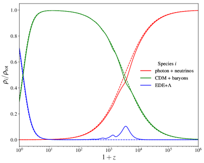
Figure 1: Densities of different components at different redshifts for EDE (full curves) and the standard $\Lambda$CDM model (dashed curves). Oscillating early dark energy density (blue curve) peaks at $z\sim 3500$ when it contributes $\sim 10\%$ to the total density. Its contribution quickly decreases after that.

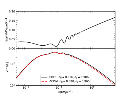
Figure 2: Bottom panel: Linear power spectrum of dark matter fluctuations at $z=0$ scaled with factor $k^{5/4}$ to reduce the dynamical range and to make the domain of BAOs $k=(0.07-0.3)h{\rm Mpc}^{-1}$ more visible. Top panel: The ratio of power spectra in our EDE model to that of the standard $\Lambda$CDM model. The amplitude of fluctuations in our EDE model is always larger than in $\Lambda$CDM though the differences at long wavelengths $\mbox{${\,\hbox{\hbox{$<$}\kern-8.00003pt\lower 4.30554pt\hbox{$\sim$}}\,}$}0.1h{\rm Mpc}^{-1}$ are only (2–3)%. The differences increase at large $k$ and become substantial ($\sim 20\%$) on galactic scales $k\mbox{${\,\hbox{\hbox{$>$}\kern-8.00003pt\lower 4.30554pt\hbox{$\sim$}}\,}$}5h{\rm Mpc}^{-1}$.

Table 1: Parameters of cosmological models.

Parameter	EDE	$\Lambda$CDM	$\Lambda$CDM
	SPA20	MultiDark-Planck13	CMB-Planck18
$\Omega_{\rm m}$	0.293	0.307	0.315$\pm 0.007$
$\Omega_{\rm cold}h^{2}$	0.132	0.119	0.120 $\pm 0.001$
$\Omega_{\rm bar}h^{2}$	0.0225	0.0221	0.0224$\pm 0.0001$
$H_{\rm 0}$ [$\rm{km\,s}^{-1}$$\rm{Mpc}^{-1}$]	72.81	67.77	67.36$\pm 0.54$
$n_{\rm s}$	0.986	0.965	0.965$\pm 0.004$
$\sigma_{8}$	0.836	0.820	0.811$\pm 0.006$
Age [Gyr]	13.032	13.825	13.797$\pm 0.023$
$z_{\rm drag}$	1061.28	1059.09	1059.94$\pm 0.30$
$r_{\rm drag}$ [Mpc]	140.1	147.8	147.1$\pm 0.3$

Table 2: Numerical and cosmological parameters of different simulations. The columns give the simulation identifier, cosmology, the size of the simulated box in $h^{-1}\,{\rm Mpc}$, the number of particles, the mass per simulation particle $m_{p}$ in units of $h^{-1}\,M_{\odot}$, the mesh size $\mbox{$N_{\rm g}$}^{3}$, the gravitational softening length $\epsilon$ in units of $h^{-1}\,{\rm Mpc}$, the number of time-steps $N_{\rm step}$, initial redshift, and the number of realizations $N_{r}$. Additional smaller-scale simulations are discussed in §6.

Simulation	Cosmology	Box	particles	$m_{p}$mmm	$\mbox{$N_{\rm g}$}^{3}$	$\epsilon$ m	$N_{\rm s}$	$z_{\rm init}$	$N_{r}$
EDE0.5	EDE	5003	20003	$1.3\times 10^{9}$	70003	0.071	253	150	5
EDE1	EDE	10003	20003	$1.0\times 10^{10}$	70003	0.143	136	100	16
EDE2A	EDE	20003	20003	$8.3\times 10^{10}$	70003	0.285	130	150	6
EDE2B	EDE	20003	20003	$8.3\times 10^{10}$	40003	0.500	130	150	210
$\Lambda$CDM0.5	MultiDark	5003	20003	$1.3\times 10^{9}$	70003	0.071	253	150	5
$\Lambda$CDM1	MultiDark	10003	20003	$1.1\times 10^{10}$	70003	0.143	136	100	30
$\Lambda$CDM2A	MultiDark	20003	20003	$8.3\times 10^{10}$	70003	0.285	130	100	15
$\Lambda$CDM2B	MultiDark	20003	20003	$8.3\times 10^{10}$	40003	0.500	130	150	210

2 Simulations

Most of the results presented in this paper are based on new cosmological $N$-body simulations. The simulations were carried out with the parallel Particle-Mesh code glam   (Klypin & Prada, 2018). Because the glam   code is very fast, we have done many realizations of the simulations with the same cosmological and numerical parameters that only differ by the initial random seed. A large number of realizations is quite important because the differences between EDE and $\Lambda$CDM models are not very large. This is especially true on long wavelengths $k\mbox{${\,\hbox{\hbox{$<$}\kern-8.00003pt\lower 4.30554pt\hbox{$\sim$}}\,}$}0.1\mbox{$h$Mpc${}^{-1}$}$ where the difference in the power spectra is just $\sim 2$%. So, one needs many realizations to reduce the cosmic variance and see the real differences.

All the glam   simulations were started at initial redshift $z_{\rm init}=100$ or $z_{\rm init}=150$ using the Zeldovich approximation. Table 2 presents the numerical parameters of our simulation suite: box-size, number of particles, particle mass $m_{p}$, number of mesh points $N_{g}^{3}$, cell-size of the density/force mesh $\epsilon$, the number of time-steps $N_{\rm step}$, and the number of realizations $N_{r}$.

The glam   code is very fast as compared with high-resolution codes such as gadget (Springel, 2005) or ART (Kravtsov et al., 1997). For example, our most expensive simulations EDE_0.5 and $\Lambda$CDM_0.5 used just $\sim 2500$ cpu-hours on a dual Intel Platinum 8280M computational node, which is just 2 days of wall-clock time. The limiting factor of glam   simulations is the force resolution $\epsilon$. It is defined by the cell size - the ratio of the box size $L$ to the mesh size $N_{g}$: $\epsilon=L/N_{g}$. So, the larger the mesh size $N_{g}$, the better is the resolution. Klypin & Prada (2018) give detailed analysis of convergence and accuracies of the glam    code. Just as with any Particle-Mesh code, the resolution is defined by the available memory: the larger the memory, the better the resolution. We use computational nodes each with 1.5Tb RAM and two Intel Platinum 8280M processors with combined 56 cores.

We use a spherical overdensity (SO) halo finder, which is a stripped down variant of the Bound Density Maxima (BDM) halo finder (Klypin et al., 2011; Knebe et al., 2011). Limited force resolution does not allow subhalos to survive in virialized halos. This is why we study only distinct halos (those that are not subhalos) in the present paper.

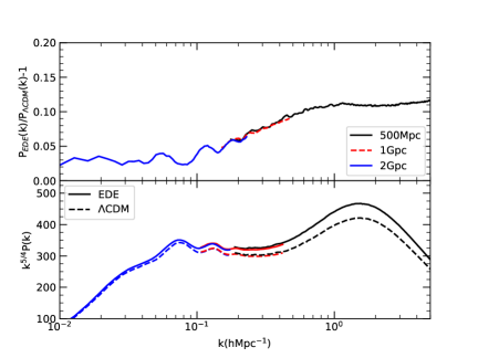
Figure 3: Similar to Figure 2 but for nonlinear evolution at $z=0$. Results from different box sizes and resolutions nicely match in overlapping regions. Nonlinear evolution dramatically changes the shape of the power spectrum at small scales. The BAO peaks are slightly damped, broadened and shifted. To some degree the nonlinear effects reduce the differences between the models, but they do not wipe them out.

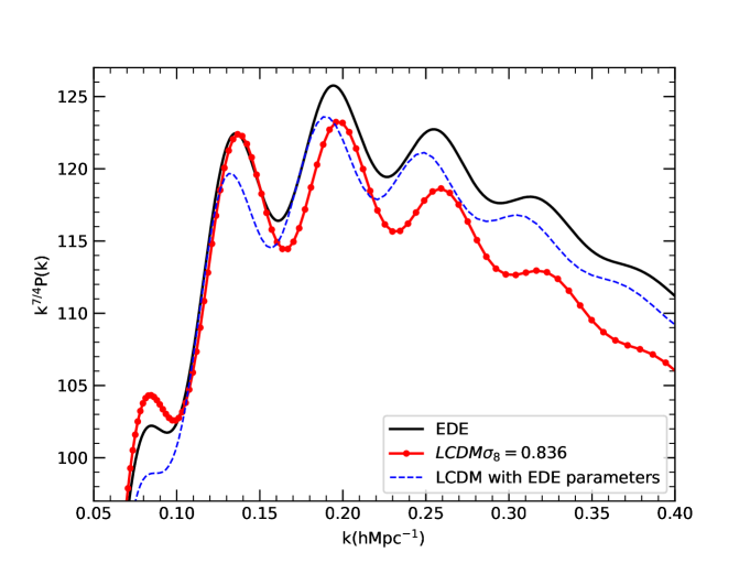
Figure 4: Linear power spectra, scaled with a factor k^7/4, for the EDE (solid line) and $\Lambda$CDM (dot-solid line) models in the BAO domain. A third $\Lambda$CDM model with the same cosmological parameters as EDE but without the early dark matter component is also shown (dashed line). All models were normalized to have the same $\sigma_{8}=0.836$ to appreciate clearly the overall shape and acoustic oscillation features differences.

3 Power Spectra

Figure 2 shows the $z=0$ linear power spectra of fluctuations in the EDE and $\Lambda$CDM models. Differences between power spectra of fluctuations are relatively small. On long wavelengths ($k\mbox{${\,\hbox{\hbox{$<$}\kern-8.00003pt\lower 4.30554pt\hbox{$\sim$}}\,}$}0.1\mbox{$h$Mpc${}^{-1}$}$) the differences are mostly explained by the normalizations: $\left[\sigma_{8}(EDE)/\sigma_{8}(\mbox{$\Lambda$CDM})\right]^{2}=1.039$. The differences increase on small scales and become substantial. For example, at $k=5\mbox{$h$Mpc${}^{-1}$}$ the amplitude of fluctuations in the EDE model is 17% bigger than in the $\Lambda$CDM model.

The reason for this increase comes from the differences in the slope $n_{s}$ of the primordial power spectra. At first sight the difference of 0.02 in the slope seems to be small. However, it results in large differences in amplitude when one compares waves that differ dramatically in wavelength: 15% for waves that differ by a factor of 1000 in wavelength. A more subtle effect is related to the halo mass function, which depends not only on the amplitude of fluctuations but also on the slope of the power spectrum.

The domain of BAOs ($k=0.07-0.3\mbox{$h$Mpc${}^{-1}$}$) is also different in the models. At first glance, the wiggles that are clearly seen in the top panel of Figure 2 are the familiar BAOs. They are not, though they are related to BAOs. If the positions of the BAO peaks were the same, there would not have been wiggles in the ratio of the power spectra. Without the early dark energy component the position of BAO peaks is mostly defined by $\Omega_{\rm bar}/\Omega_{\rm m}$ and $\Omega_{\rm m}h^{2}$ (Eisenstein & Hu, 1998). There is an additional effect in EDE models due to the fact that the early dark energy changes the dynamics of acoustic waves before the recombination. So, the very presence of the wiggles tells us that BAO peaks happen at different wavenumbers: in the EDE models the BAOs are shifted to slightly smaller wavenumbers.

Nonlinear evolution modifies the power spectra. Figure 3 shows results of our simulations at redshift $z=0$. Results from different box sizes and resolutions nicely match each other in overlapping regions. As the result, we stack together different simulations and extend the range of resolved scales.

As clearly seen in Figure 3 the nonlinear evolution dramatically changes the shape of the power spectrum: at $k\mbox{${\,\hbox{\hbox{$>$}\kern-8.00003pt\lower 4.30554pt\hbox{$\sim$}}\,}$}0.5\mbox{$h$Mpc${}^{-1}$}$ the fluctuations are much larger as compared with the linear regime. The bump at $k\sim 1.5\mbox{$h$Mpc${}^{-1}$}$ corresponds to mass $M=(4\pi/3)\Omega_{m}\rho_{\rm cr}(\lambda/2)^{3}\approx 10^{13}\mbox{$h^{-1}M_{\odot}$ }$ – scale of large galaxies like our Milky Way. So, the bump is a manifestation of collapsing dark matter halos.

To some degree the nonlinear effects reduce the differences between the models at strongly non-linear regime $k\mbox{${\,\hbox{\hbox{$>$}\kern-8.00003pt\lower 4.30554pt\hbox{$\sim$}}\,}$}1\mbox{$h$Mpc${}^{-1}$}$. Here the ratios of the power spectra are nearly constant 10% – a marked deviation from the linear spectra shown in Figure 2. This nearly constant ratio of non-linear spectra produces small and hardly detectable differences in the abundance of halos at $z=0$. Note that at larger redshifts the differences are larger than at $z=0$ because the nonlinearities are smaller.

The power spectra in the domain of BAOs are also affected by nonlinearites, but in a more subtle way. The BAO peaks are slightly damped, broadened and shifted: effects that are well understood and well studied (e.g., Eisenstein et al., 2007; Angulo et al., 2008; Prada et al., 2016), see Section 4 for a detailed study. At even larger scales $k\mbox{${\,\hbox{\hbox{$<$}\kern-8.00003pt\lower 4.30554pt\hbox{$\sim$}}\,}$}0.05\mbox{$h$Mpc${}^{-1}$}$ the fluctuations are still in the nearly linear regime.

The fact that nonlinear evolution reduces differences between EDE and $\Lambda$CDM models is a welcome feature. We know that at low redshifts $z\mbox{${\,\hbox{\hbox{$<$}\kern-8.00003pt\lower 4.30554pt\hbox{$\sim$}}\,}$}0.5$ the $\Lambda$CDM model reproduces the observed clustering of galaxies in samples such as SDSS and BOSS (Guo et al., 2015; Rodríguez-Torres et al., 2016; Kitaura et al., 2016). So, too large deviations from $\Lambda$CDM may point to problems. Nevertheless, though relatively small, the deviations still exist and potentially can be detected. The fact that nonlinear evolution reduces the differences implies that one also expects larger differences at higher redshifts. Indeed, this is what we find from analysis of halo abundances discussed below.

4 Baryonic Acoustic Oscillations

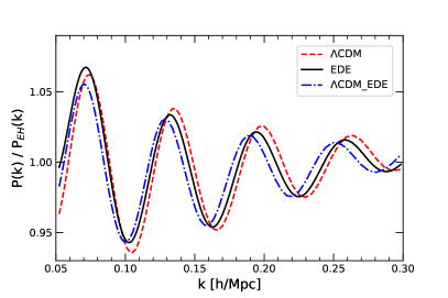
Figure 5: BAO wiggles in the linear power spectrum for the three cosmological models: EDE (solid line), $\Lambda$CDM (dashed line), and $\Lambda$CDM_EDE (dot-solid line) with the same cosmological parameters as EDE. The plot shows the deviations of the power spectra from that without baryonic oscillations (Eisenstein & Hu, 1998). As compared with $\Lambda$CDM the BAO peaks in EDE are systematically shifted by $1.8\%$ to smaller wavenumbers, and in the case of $\Lambda$CDM_EDE by $4.4\%$ to smaller wavenumbers.

Figure 4 displays the linear power spectra for the EDE (solid line) and two $\Lambda$CDM models in the domain of the BAO features. In order to appreciate more clearly their overall P(k) shapes and BAO differences, the two $\Lambda$CDM models have been normalized to have the same $\sigma_{8}=0.836$ as that of EDE. One $\Lambda$CDM model is otherwise the MultiDark-Planck one (dot-solid line). The other $\Lambda$CDM model (named $\Lambda$CDM_EDE, dashed line) has the same cosmological parameters as EDE but without the effects of the early dark energy component.

As compared with $\Lambda$CDM  the BAO peaks in the EDE model are systematically shifted to smaller wavenumbers. This reflects the fact that the acoustic sound horizon has a larger value due to the faster expansion before the epoch of recombination. On the other hand, the sound horizon $r_{\rm d}$ in the EDE cosmology is smaller as compared to the $\Lambda$CDM_EDE model ($r_{d}=143.92$ Mpc) despite both cosmologies having the same cosmological parameters, and hence the BAO peaks in the latter are shifted towards larger scales. In the concordance $\Lambda$CDM models the positions of the acoustic peaks are defined by $\Omega_{\rm m}h^{2}$ and $\Omega_{\rm bar}h^{2}$ (see Aubourg et al., 2015). But the propagation of acoustic waves is different in EDE models, as the EDE boosts the Hubble rate around $z_{\rm eq}$ and thus these two cosmological parameters no longer define the BAO peak positions.

The relative difference between the BAO wiggles in the three cosmologies is better seen in Figure 5, where we show the deviations for each linear power spectrum from that without BAO features obtained from the (Eisenstein & Hu, 1998) “non-wiggle” P_nw(k) fitting formula. The BAO shifts among the three cosmological models are clearly visible, and systematically shifted towards smaller wavenumbers by $1.8\%$ for EDE and $4.4\%$ for $\Lambda$CDM_EDE with respect to the $\Lambda$CDM BAO positions. This is expected given their corresponding acoustic sound horizon ratios $r_{d}/r^{\rm fid}_{d}$, where $r^{\rm fid}_{d}$ is the sound horizon of our fiducial cosmology, the $\Lambda$CDM model.

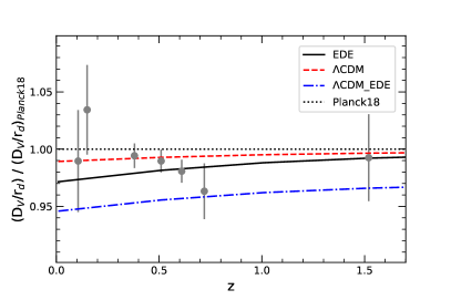
Figure 6: Acoustic-scale distance measurements relative to the prediction from Planck TT,TE,EE+lowE+lensing in the base-$\Lambda$CDM model (see Table 1, Planck Collaboration et al., 2018). The symbols and $1\sigma$ error bars correspond, in increasing redshift order, to the isotropic BAO measurements D_V(z)/r_d from the 6dFGRS (Beutler et al., 2011), the SDSS-MGC (Ross et al., 2015), BOSS DR12 LRGs (at $z=$ 0.38, 0.51, and 0.61, Alam et al., 2017), eBOSS DR14 LRGs (Bautista et al., 2018) and eBOSS DR14 QSOs (Ata et al., 2018). The curves provide the model predictions from EDE (solid), MultiDark-$\Lambda$CDM (dashed), and $\Lambda$CDM with the same EDE cosmological parameters (dashed-dotted).

The BAO position in the spherically averaged two-point clustering statistics, and hence the acoustic-scale distance measurements obtained from large galaxy redshift surveys, are based on the constraints of the stretch or dilation parameter $\alpha$ defined as,

$$\alpha\equiv\frac{(D_{\rm V}(z)/r_{\rm d})}{(D^{\rm fid}_{\rm V}(z)/r^{\rm fid}_{\rm d})},$$ (1)

where $D_{\rm V}(z)\equiv[cz(1+z)^{2}D^{2}_{A}H^{-1}(z)]^{1/3}$ is the dilation distance (Eisenstein et al., 2005), $D_{A}$ is the angular diameter distance and $H(z)$ is the Hubble parameter. The stretch parameter $\alpha$ is measured from the best-fit model to the observed isotropic power spectrum or correlation function on the scale range $0.05\,h/{\rm Mpc}\lesssim k\lesssim 0.3\,h/{\rm Mpc}$ (see, e.g., Anderson et al., 2014; Ross et al., 2015). The latest and more accurate acoustic-scale distance $D_{\rm V}/r_{\rm d}$ measurements, relative to the prediction from $Planck$ TT,TE,EE+lowE+lensing (CMB) in the base-$\Lambda$CDM model (i.e., our fiducial MultiDark-Planck13 cosmology, see Table 1) are shown in Figure 6. The curves in Figure 6 correspond to the model predictions from EDE (solid), MultiDark-$\Lambda$CDM (dashed), and $\Lambda$CDM with the same EDE cosmological parameters (dashed-dotted). We conclude that EDE and our $\Lambda$CDM cosmology models both agree well with the observations.

The effect of early dark energy clearly shows up at later epochs, having its maximum difference $\sim 2\%$ at $z=0$ as compared to $\Lambda$CDM. The upcoming DESI and Euclid experiments with sub-percent accuracy on the acoustic scale measurements will be able to test models such as the EDE one considered in this work. It is interesting to note that $\Lambda$CDM_EDE, despite having the same cosmological parameters as EDE but not the same sound horizon scale, predicts $\alpha$ that differs substantially at all redshifts by about $4\%$) (see Figure 6).

Table 3: Mean values of the BAO shift and damping at different redshifts obtained from the best-fit $\alpha$ and $\Sigma_{nl}$ parameters of the $\sim 200$ realizations of EDE_2B and $\Lambda$CDM_2B real-space power spectra (see Table 2). The damping computed from linear theory $\Sigma^{th}_{nl}$ for each cosmology is also listed for comparison.

		$\Lambda$CDM			EDE
redshift	$\alpha-1$[%]	$\Sigma_{nl}$ (Mpc/h)	$\Sigma_{nl}^{th}$	$\alpha-1$[%]	$\Sigma_{nl}$ (Mpc/h)	$\Sigma_{nl}^{th}$
4.079	$0.061\pm 0.020$	$2.089\pm 0.052$	2.101	$0.060\pm 0.019$	$2.090\pm 0.055$	2.170
2.934	$0.080\pm 0.022$	$2.745\pm 0.039$	2.703	$0.078\pm 0.020$	$2.787\pm 0.042$	2.791
1.940	$0.115\pm 0.024$	$3.650\pm 0.032$	3.584	$0.110\pm 0.023$	$3.729\pm 0.033$	3.699
1.799	$0.123\pm 0.024$	$3.823\pm 0.031$	3.756	$0.117\pm 0.023$	$3.907\pm 0.032$	3.876
1.553	$0.139\pm 0.025$	$4.162\pm 0.030$	4.095	$0.132\pm 0.024$	$4.255\pm 0.031$	4.224
1.256	$0.165\pm 0.027$	$4.650\pm 0.029$	4.589	$0.154\pm 0.027$	$4.755\pm 0.030$	4.731
1.021	$0.182\pm 0.026$	$5.095\pm 0.026$	5.063	$0.176\pm 0.029$	$5.228\pm 0.030$	5.215
0.775	$0.228\pm 0.032$	$5.688\pm 0.029$	5.656	$0.205\pm 0.032$	$5.813\pm 0.030$	5.820
0.500	$0.280\pm 0.036$	$6.456\pm 0.030$	6.465	$0.247\pm 0.036$	$6.591\pm 0.031$	6.641
0.244	$0.345\pm 0.042$	$7.306\pm 0.033$	7.377	$0.297\pm 0.042$	$7.450\pm 0.034$	7.560
0.007	$0.390\pm 0.043$	$8.184\pm 0.033$	8.354	$0.352\pm 0.049$	$8.343\pm 0.037$	8.536

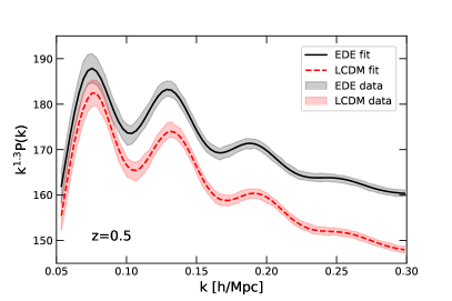
Figure 7: Mean, and standard deviation, of the dark matter power spectra at $z=0.5$ obtained from the ensemble of $\sim 200$ EDE and $\Lambda$CDM GLAM simulations. The solid (dashed) lines correspond to the best-fit model given by Eq. 2 in the wavenumber range $0.05<k<0.3$ h Mpc^-1 for the EDE ($\Lambda$CDM) data.

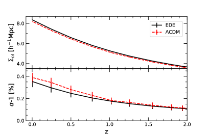
Figure 8: Non-linear evolution of the BAO shift (bottom panel) and damping (top panel) for the isotropic dark matter power spectrum in our EDE_2B and $\Lambda$CDM_2B simulations. The displayed mean values, and $1\sigma$ uncertainties, of $\alpha$ and $\Sigma_{nl}$, and given in Table 6, are estimated from the ensemble of individual shifts and damping parameters measured from fitting each of the power spectra, using Eq. 2, of the EDE and $\Lambda$CDM GLAM simulations.

The acoustic-scale distance measurements up to $z=1.5$ displayed in Figure 6 include density-field reconstruction of the BAO feature, which is used to partially reverse the effects of non-linear growth of structure formation (see Anderson et al., 2012; Padmanabhan et al., 2012). The shape of the linear matter power spectrum $P(k)$ is distorted by the nonlinear evolution of density fluctuations, redshift distortions and galaxy bias even at large-scales $k<0.2\,\mbox{$h$Mpc${}^{-1}$}$. As mentioned above, the shift parameter $\alpha$ yields the relative position of the acoustic scale in the power spectrum (or two-point correlation function) obtained from the data (or simulations) with respect to the adopted $P(k)$ model.

Here we study the non-linear shift and damping of acoustic oscillations up to redshift $z=4$ for dark matter in our ensemble of $\sim 200$ EDE and $\Lambda$CDM GLAM $N-$body simulations. Figure 7 shows the spherically-averaged power spectra at $z=0.5$ in real-space drawn for both cosmologies in the domain of the BAO features. We measure the shift of the BAO relative to linear theory by following a similar methodology as that presented in Seo et al. (2008), and implemented in Anderson et al. (2014) to measure the BAO stretch parameter in the BOSS data. The non-linear dark matter power spectrum with wiggles is modeled by damping the acoustic oscillation features of the linear power spectrum assuming a Gaussian with a scale parameter $\Sigma_{\rm nl}$ which accounts for the BAO broadening due to nonlinear effects (e.g. Eisenstein et al., 2007). We use the functional form:

$$\begin{split}P(k)=P_{\rm sm}(k)\left[1+\left(\frac{P_{\rm lin}(k/\alpha)}{P_{\rm nw}(k/\alpha)}-1\right)e^{-\frac{1}{2}(k/\alpha)^{2}\Sigma_{nl}^{2}}\right]\,,\end{split}$$ (2)

where $P_{\rm lin}$ is the linear power spectrum generated with CAMB for each cosmology model, and $P_{sm}$ is the smooth "BAO-free" power spectrum modelled as $P_{sm}=P_{\rm nw}(k)+A(k)$ with $P_{\rm nw}(k)$ being the "de-wiggled" (Eisenstein & Hu, 1998) spectrum template and $A(k)$ accounting for the non-linear growth of the broad-band matter power spectrum expressed in the form of simple power-law polynomial terms $A(k)=a_{1}k+a_{2}+A_{3}/k+A_{4}/k^{2}+A_{5}/k^{3}$ (Anderson et al., 2014). The shift and damping of the acoustic oscillations, measured by $\alpha$ and $\Sigma_{nl}$, are considered free parameters in our model.

We then perform the fit of the power spectrum $P(k)$ drawn from each of our GLAM simulations over the wavenumber range $0.05<k<0.3$ h Mpc^-1 for several redshifts. The solid (dashed) line in Figure 7 corresponds to the best-fit power spectrum model given by using Eq. 2 for the EDE ($\Lambda$CDM) simulation data. The shift and damping of the BAO features in both cosmologies is similar as can be seen from the plot. The mean values, and $1\sigma$ uncertainties, of the $\alpha$ and $\Sigma_{nl}$ parameters obtained from the best-fit to each of the EDE and $\Lambda$CDM GLAM power spectra are provided in Table 3 up to $z=4$. The nonlinear damping estimated from perturbation theory for each cosmology is also listed, and shows a remarkable agreement better than $2\%$ over all redshifts with that measured from our model fits to the simulation data.

Our shift results for the acoustic scale towards larger $k$, relative to the linear power spectrum, and damping values obtained from our analysis are in good agreement with previous works for $\Lambda$CDM (e.g. Crocce & Scoccimarro, 2008; Seo et al., 2010; Prada et al., 2016). Figure 8 demonstrates that the non-linear evolution of the BAO shift (bottom panel) and damping (top panel) for the isotropic dark matter power spectrum in both EDE and $\Lambda$CDM cosmologies display small differences, with the BAO features being less affected by the non-linear growth of structure formation. Moreover, Bernal et al. (2020) shows that the $\Lambda$CDM-assumed templates used for anisotropic-BAO analyses can be used in EDE models as well.

A summary of our BAO results can also be shown in configuration space. In Figure 9 we see that the BAO peak in the EDE linear correlation function (right panel) is slightly shifted by $\sim 2\%$ to larger radii as compared with the $\Lambda$CDM model, as expected from their different values of the sound horizon scale at the drag epoch. The impact of non-linear evolution broadens the BAO peaks but it does not reduce the shift differences between EDE and $\Lambda$CDM.

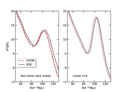
Figure 9: Right panel: Linear correlation function of dark matter at $z=0$ on large scales. We plot the correlation function $\xi(R)$ scaled with $R^{2}$ to remove the main trend of the correlation function. The correlation function in the EDE model is slightly shifted by $\sim 2\%$ to larger radii as compered with the $\Lambda$CDM model. Left panel: Nonlinear correlation function at $z=0$. As compared to the linear $\xi(R)$, the BAO peak in the nonlinear regime slightly shifts to smaller values and becomes wider with smaller amplitude – effects that are well known and well understood. Nonlinear effects do not reduce differences between EDE and $\Lambda$CDM models.

5 Halo abundances

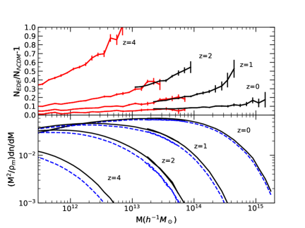
Figure 10: Halo mass function at redshifts $z=0-4$. Full curves in the bottom panel are for the EDE simulations and dashed curves are for the $\Lambda$CDM simulations. The smaller box and better resolution simulations EDE_0.5 and $\Lambda$CDM_0.5 are used for masses below $M\mbox{${\,\hbox{\hbox{$<$}\kern-8.00003pt\lower 4.30554pt\hbox{$\sim$}}\,}$}10^{14}\mbox{$h^{-1}$Mpc}$. They are shown as red curves in the top panel. Larger box and lower resolution simulations EDE_2A and $\Lambda$CDM_2A (black curves in the top panel) are used for massive halos with $M\mbox{${\,\hbox{\hbox{$>$}\kern-8.00003pt\lower 4.30554pt\hbox{$\sim$}}\,}$}2\times 10^{13}\mbox{$h^{-1}$Mpc}$. At $z=0$ halo abundances are very similar for the models: EDE predicts $\sim 10\%$ more of the most massive clusters $M\approx 10^{15}\mbox{$h^{-1}M_{\odot}$ }$ and 1%-2% more of galaxy-size halos with $M\approx 10^{12-13}\mbox{$h^{-1}M_{\odot}$ }$. The differences in abundances increase substantially with the redshift.

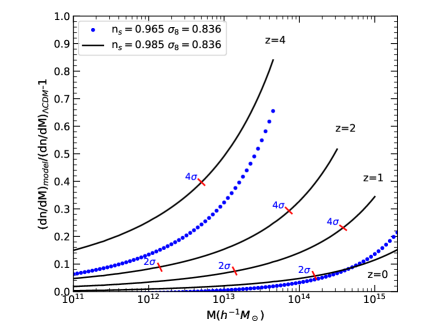
Figure 11: Analytical estimates of the ratio of halo abundances of different models relative to the abundance in the $\Lambda$CDM model. The Despali et al. (2016) approximation is used to make the predictions. Dotted curves for $z=0$ and $z=4$ show effects due to the increase of just normalization from $\sigma_{8}=0.820$ in $\Lambda$CDM to $\sigma_{8}=0.836$ (as in the EDE model). The full curves are for the model with increased slope $n_{s}=0.985$ (as compared to $n_{s}=0.965$ in $\Lambda$CDM) and the increased $\sigma_{8}=0.836$. Small lines mark positions of peaks of given $\nu$ height. As expected, the curves start to go up steeply when halos become high peaks of the Gaussian field. The analytical models qualitatively explain the main differences between the EDE and $\Lambda$CDM models, although they underpredict the magnitude of the real differences observed in Figure 10.

To study halo mass functions we use simulations with 500$h^{-1}$Mpc and 1000$h^{-1}$Mpc boxes and mesh size $N_{g}=7000$. Simulations with larger 2$h^{-1}$Gpc boxes have lower mass and force resolutions – not sufficient for analysis of galaxy-mass halo abundances.

Halos in simulations were identified with the Spherical Overdensity halofinder BDM (Klypin et al., 2011; Knebe et al., 2011) that uses the virial overdensity definition of Bryan & Norman (1998). The resolution was not sufficient for identifying subhalos, so only distinct halos are studied.

Figure 10 shows the halo mass function at different redshifts. The EDE model predicts more halos at any redshift, but the difference is very small at $z=0$: a 10% effect for very massive clusters $M\approx 10^{15}\mbox{$h^{-1}M_{\odot}$ }$ and just 1% for Milky Way-mass halos with $M=10^{12}\mbox{$h^{-1}M_{\odot}$ }$. These differences hardly make any impact on predicted statistics of galaxies and clusters with observational uncertainties and theoretical inaccuracies being larger than differences in halo abundances.

The situation is different at larger redshifts: the number of halos in EDE is substantially larger than in $\Lambda$CDM. For example, the EDE model predicts about 50% more massive clusters of mass $M=(3-5)\times 10^{14}\mbox{$h^{-1}M_{\odot}$ }$ at $z=1$. The differences increase even more at larger redshifts. For example, the EDE model predicts almost twice more galaxy-size halos with $M>3\times 10^{12}\mbox{$h^{-1}M_{\odot}$ }$ at redshift $z=4$. These are interesting predictions that can potentially be tested by comparing with abundances of high redshift $z\mbox{${\,\hbox{\hbox{$>$}\kern-8.00003pt\lower 4.30554pt\hbox{$\sim$}}\,}$}1$ clusters of galaxies (e.g., Bayliss et al., 2014; Gonzalez et al., 2015; Bocquet et al., 2019), abundances of massive galaxies and black holes at $z>4$ (e.g., Haiman & Loeb, 2001; Stefanon et al., 2015; Behroozi & Silk, 2018; Carnall et al., 2020), and clustering of high-redshift galaxies (Harikane et al., 2016, 2018; Endsley et al., 2020).

Another consequence of the increased mass function in EDE is earlier collapse times. More halos in EDE at higher redshifts implies that halos of a given mass $M$ form earlier in the EDE model. Because the Universe is denser at those times, so are the halos. At later times the accretion of dark matter onto the halo gradually builds the outer halo regions resulting in increasing halo concentration (e.g., Bullock et al., 2001). Thus denser central regions in EDE models should lead to more concentrated halos.

At first sight our results on the halo mass functions are puzzling. Halo mass functions are defined by the amplitude of perturbations $\sigma(M,z)$. However, the normalization of the perturbations $\sigma_{8}$ is just 2% different in the EDE model. Why do we see large deviations in the halo abundances? The evolution of the mass function is defined by the growth rate of fluctuations, which in turn is defined by $\Omega_{m}$, which is nearly the same for EDE and $\Lambda$CDM models. In this case why do we see large evolution of the differences between the models? In order to have some insights on the issue, we use analytical estimates of the halo mass function that allow us to change parameters and see their effects.

Specifically, we use the Despali et al. (2016) approximation for virial halo mass function at different redshifts. By itself the approximation is not accurate enough to reliably measure the differences between EDE and $\Lambda$CDM models. However, it is good enough to study trends and to probe effects of different parameters.

According to the theory (e.g., Bond et al., 1991; Sheth & Tormen, 1999), the halo mass function $n(M,z)$ is a function of $\sigma(M,z)$ – the $rms$ of the linear density field smoothed with the top-hat filter of radius $R_{f}$ corresponding to the average mass $M$ inside a sphere of radius $R_{f}$: $M=(4\pi/3)\rho_{m}R_{f}^{3}$. Spherical fluctuations that in the linear approximation exceed a density threshold $\delta_{\rm cr}\approx 1.68$ in the real nonlinear regime collapse and form dark matter halos. The halo mass function

$$\frac{dn}{dM}=f(\sigma)\left[\frac{\Omega_{m}\rho_{\rm crit}}{M^{2}}\right]\frac{d\ln\sigma}{d\ln M}$$ (3)

can be written in a form that depends mostly on one parameter – the relative height of the density peak $\nu$ defined as:

$$\nu=\frac{\delta_{\rm cr}}{\sigma(M,z)}.$$ (4)

There are different approximations for function $f(\sigma)$. We start with the Press-Schechter approximation because it is easy to see the main factors defining the mass function:

$$\left(\frac{M^{2}}{\Omega_{m}\rho_{\rm crit}}\right)\frac{dn}{dM}=\sqrt{\frac{2}{\pi}}\nu\exp\left(-\frac{\nu^{2}}{2}\right)\frac{d\ln\sigma}{d\ln M}.$$ (5)

When $\nu$ is small ($\nu\mbox{${\,\hbox{\hbox{$<$}\kern-8.00003pt\lower 4.30554pt\hbox{$\sim$}}\,}$}1$), the Gaussian term is close to unity, and the amplitude of the mass functions is linearly proportional to $\nu$, which, in turn, is inversely proportional to the normalization $\sigma_{8}$. This explains why the EDE mass function is just $\sim 1\%-2\%$ larger than in $\Lambda$CDM at small $M$ and at $z=0$: we are dealing with small $\nu$ peaks of the Gaussian density field. As mass increases, the rms of fluctuations $\sigma(M)$ decreases, and eventually $\nu$ becomes large. In this case the Gaussian term dominates, and we expect a steep decline of $dn/dM$. In this regime the ratio of mass functions is equal to $\approx\exp(\alpha\nu^{2})$, where $\alpha=(\sigma_{8,\rm EDE}/\sigma_{8,\rm\mbox{$\Lambda$CDM}})-1\approx 0.02$. For example, for $4\sigma$ fluctuations $\nu=4$, we expect a $\sim 40\%$ difference. In other words, for high-$\nu$ peaks a small change in the amplitude of fluctuations produces a very large change in the halo abundance. This is exactly what we see in Figure 10 at large redshifts.

In practise, we use a better approximation for the halo mass function provided by Despali et al. (2016). We find that the approximation is very accurate at low redshifts with the errors less than $\mbox{${\,\hbox{\hbox{$<$}\kern-8.00003pt\lower 4.30554pt\hbox{$\sim$}}\,}$}3\%$ for masses $M_{h}>10^{12}\mbox{$h^{-1}M_{\odot}$ }$. However, the errors increase with the redshift, becoming $\approx 12\%$ at $z=4$ for the $\Lambda$CDM model. The errors also depend on cosmology: at $z=4$ the error for the EDE model is $\approx 30\%$. While not very accurate, the approximation can be used for qualitative analysis.

We are mostly interested in effects of modification of the amplitude $\sigma_{8}$ and in changes of the slope of the spectrum $P(k)$. For the base model we use $\Lambda$CDM with $\sigma_{8}=0.820$. We start with increasing the amplitude to the same value $\sigma_{8}=0.836$ as in the EDE model. When doing this, we take the same shape of spectrum as in $\Lambda$CDM and increase the normalization. Dotted curves in Figure 11 show how the mass function changes due to the increased $\sigma_{8}$. As expected, the high-$\sigma_{8}$ model has more halos and the difference increases with mass and with the redshift. However, the shape of the mass function ratios is too steep as compared with the $N$-body simulations. Compare, for example, the $z=0$ curves in Figure 10 and Figure 11. Also, the magnitude of the effect is much smaller at $z=4$ as compared with what it should be.

Now we also change the slope of the power spectrum from $n_{s}=0.965$ to the same value $n_{s}=0.985$ as in the EDE model while keeping the same high normalization $\sigma_{8}$. Because the radius $R_{f}=8\mbox{$h^{-1}$Mpc}$ of the top-hat filter in the $\sigma_{8}$ definition was chosen such that the abundance of massive clusters with $M\approx 10^{15}\mbox{$h^{-1}M_{\odot}$ }$ should stay approximately constant, keeping the same $\sigma_{8}$ means that cluster abundance does not change much. At the same time a steeper slope of $P(k)$ means that the amplitude of fluctuations increases for small halos. As the result, the full curves for tilted and high-$\sigma_{8}$ models in Figure 11 are flatter producing more halos with small mass.

In Figure 11 we also mark positions of peaks of given $\nu$ height. As expected, the curves start to steeply go up when halos become high peaks of the Gaussian field.

In summary, the EDE model predicts quite similar ($1-10\%$) halo abundance as $\Lambda$CDM at low redshifts, significantly increasing at higher redshifts. Most of the increase is due to the change $\Delta n_{s}=0.02$ in the slope of the power spectrum with the increase in $\sigma_{8}$ playing an additional role. These results are well understood in the framework of the theory of the halo mass function, although the analytical approximation by Despali et al. (2016) fails to reproduce the results accurately with errors up to $\sim 30\%$ being redshift- and model-dependent.

6 Halo abundances and clustering at high redshifts

Results discussed in the previous section show a remarkable increase with redshift in halo abundances in the EDE model (relative to the $\Lambda$CDM model). Here, we study predictions for even larger redshifts. We focus on two issues: (a) the abundance of small halos at the epoch of recombination ($z=6-10$) and (b) the clustering of halos at $z=4-6$ that are plausibly measurable with JWST (Endsley et al., 2020).

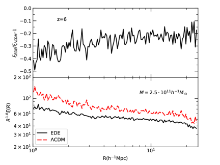
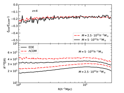
Figure 12: Correlation functions of dark matter halos at redshift $z=6$ (top panels) and $z=4$ (bottom panels). Halos above virial masses indicated in the plots were used to find the correlations and their ratios. In the distance range $R=(1-20)\mbox{$h^{-1}$Mpc}$ the correlation functions are well approximated by a power-law $\xi(R)\propto r^{-1.8}$. At each redshift halos in the EDE model are less clustered by $\sim(10-30)\%$ than halos with the same mass cut in the $\Lambda$CDMmodel – an unexpected result considering that the dark matter in the EDE model is more clustered.

We make additional simulations using smaller simulation boxes of $50\mbox{$h^{-1}$Mpc}$ and $250\mbox{$h^{-1}$Mpc}$ with $2000^{3}$ particles and force resolutions of $7\mbox{$h^{-1}$kpc}$ and $36\mbox{$h^{-1}$kpc}$ correpondingly, which is substantially better than in the $EDE_{0.5}$ and $\mbox{$\Lambda$CDM}_{0.5}$ simulations. In addition to our EDE and $\Lambda$CDM models, we also run a simulation $\mbox{$\Lambda$CDM}_{\rm low}$ with the same parameters as the $\Lambda$CDMmodel  but with lower amplitude of fluctuations $\sigma_{8}=0.75$ that is motivated by weak-lensing results (e.g., Hamana et al., 2020). Because of the smaller box size, the improved mass resolution of these simulations ($m_{p}=1.3\times 10^{6}\mbox{$h^{-1}M_{\odot}$ }$ and $m_{p}=1.6\times 10^{8}\mbox{$h^{-1}M_{\odot}$ }$) allows us to study halo abundances and halo clustering for halos with masses as low as $\sim 10^{9}-10^{10}\mbox{$h^{-1}M_{\odot}$ }$.

The abundance and clustering of such low-mass halos is particularly relevant for understanding reionization. The Universe was re-ionized between $z=6-10$ (e.g., Madau & Dickinson, 2014), and it is generally accepted that the observed population of relatively bright star-forming galaxies ($M_{\mathrm{UV}}<-17$; $M_{h}>10^{10}\mbox{$h^{-1}M_{\odot}$ }$) cannot provide enough ionizing photons (Paardekooper et al., 2015; Robertson et al., 2015; Finkelstein et al., 2019). However, fluxes from fainter galaxies may be sufficient (Robertson et al., 2015; Yung et al., 2020). The predicted ionizing flux of UV radiation depends on three factors: efficiency of star formation (especially in low-mass halos), abundance of halos of different masses at the epoch of re-ionization, and the escape fraction of photons. Theoretical estimates (Finkelstein et al., 2019; Yung et al., 2020) indicate that about 50-60% of ionizing photons were produced by (but not necessarily escaped from) galaxies hosted in halos with masses $M_{h}=10^{10}-10^{12}\mbox{$h^{-1}M_{\odot}$ }$. These estimates are based on halo abundances in the standard $\Lambda$CDM model. Most of the radiation came from galaxies hosted by halos with mass $M_{h}>10^{9}\mbox{$h^{-1}M_{\odot}$ }$ (Barkana & Loeb, 2001; Finkelstein et al., 2019).

We find that the trend of increasing halo abundance ratios persists during the epoch of re-ionization at redshifts $z=6-10$. For example, at $z=7.5$ the EDE model predicts $1.8$ times more halos with masses larger than $M=10^{10}\mbox{$h^{-1}M_{\odot}$ }$ as compared with $\Lambda$CDM. The difference with $\mbox{$\Lambda$CDM}_{\rm low}$ is even more striking: there are more than 3.7 times more halos above that mass cut in the EDE as compared with the $\mbox{$\Lambda$CDM}_{\rm low}$ model. At $z=10$, the $\mbox{$\Lambda$CDM}_{\rm low}$ model has 8.3 times fewer halos with $M>5\times 10^{9}\mbox{$h^{-1}M_{\odot}$ }$ as compared with the EDE model.

Thus, with other parameters fixed, the EDE model would predict a factor of $\sim 1.5-2$ larger ionizing fluxes as compared with the $\Lambda$CDM model. Reducing the fluctuation amplitude to $\sigma_{8}=0.75$ would result in reduction of fluxes by a factor of 3-5 compared with $\Lambda$CDM, which would be problematic.

Clustering of high-redshift galaxies is potentially an interesting way to distinguish different cosmological models. Ground observations with the Hyper Suprime-Cam (HSC) Subaru telescope (e.g., Harikane et al., 2016, 2018) and future measurements of large samples of galaxies at $z=4-6$ with JWST (Endsley et al., 2020) will bring an opportunity to combine galaxy clustering with abundances as a probe for halo masses and merging rates. Theoretical estimates indicate that the observed galaxies at those redshifts should be hosted by halos with masses in the range $M=10^{10}-10^{12}\mbox{$h^{-1}M_{\odot}$ }$ (Harikane et al., 2016, 2018; Endsley et al., 2020).

As we saw earlier, the EDE model predicts stronger dark matter clustering and larger halo abundances at high redshifts as compared with the $\Lambda$CDM model. Thus, one would naively expect that halos–and galaxies hosted by those halos–should also be more clustered. However, our simulations show that this is not the case. Here, we use distinct halos in the EDE_0.5 and $\Lambda$CDM_0.5 simulations to study clustering of halos with masses $M=(2-5)\times 10^{11}\mbox{$h^{-1}M_{\odot}$ }$. Figure 12 shows the results for halos at $z=6$ (top panels) and $z=4$ (bottom panels). Note that the smallest radius plotted, $R=1\mbox{$h^{-1}$Mpc}$, is significantly larger than the virial radii of these halos. Thus, the radii presented in the Figure are well in the domain of the two-halo term and are well resolved by the simulations.

The halo correlation functions at those redshifts and radii are nearly power-laws, $\xi(R)\approx(R/R_{0})^{\gamma}$, with slopes $\gamma\approx-1.7-1.9$, which is similar to the slope of Milky-Way-mass halos at $z=0$. The amplitudes of clustering ($R_{0}$) at high redshifts are remarkably large. For example, at $z=6$ and $M>2.5\times 10^{11}\mbox{$h^{-1}M_{\odot}$ }$, the clustering scale is $R_{0}=9.9\mbox{$h^{-1}$Mpc}$ for $\Lambda$CDM and $R_{0}=8.8\mbox{$h^{-1}$Mpc}$ for the EDE model.

Somewhat unexpectedly, the clustering of halos in the EDE model is smaller than in $\Lambda$CDM in spite of the fact that the dark matter is more strongly clustered in EDE. The differences depend on redshift and halo mass, but those dependencies are weak. Overall, at the same mass cut, halos in EDE have correlation functions $\approx 20-30\%$ smaller. When we select halos with the same cumulative number density, the differences become even smaller ($\approx 10\%$). This suggests that measuring clustering at fixed galaxy number density will not be a strong test of EDE. Instead, other mass-sensitive measures (e.g., satellite kinematics or redshift-space distortions) may be more successful probes at high redshifts.

7 Summary and Discussion

There are two main tensions between the standard $\Lambda$CDM cosmology and local observations, the Hubble tension and the $S_{8}$ tension. The EDE model considered here resolves the Hubble tension, which is that Planck-normalized $\Lambda$CDM predicts a value of the cosmological expansion rate that is smaller than local measurements by as much as 6$\sigma$. Such a large discrepancy is unlikely to be a statistical fluke. And it is probably not due to systematic errors because it is seen in different kinds of measurements, in particular Cepheid-calibrated SNe Ia giving $h=0.674\pm 0.006$ (Riess et al., 2019b, the SH0ES team) and strong-lens time delays giving $h=0.733\pm 0.018$ (Wong et al., 2020, the H0LiCOW team).

As we discussed in the Introduction, this Hubble tension can be resolved by adding a maximum of 10% of dark energy to the energy density of the universe for a brief period around the end of the radiation domination era at redshift $z\approx 3500$ (Smith et al., 2020, Figure 1). As we also discussed in the Introduction, this EDE model does not exacerbate the relatively small ($\sim 2\sigma$) $S_{8}$ tension in standard ΛCDM.

In this paper on the EDE model we have focused on the nonlinear effects on halo abundance and clustering, including the baryon acoustic oscillations. On large scales, the small differences between the linear power spectra of standard $\Lambda$CDM and our EDE model are mostly due to the different $\sigma_{8}$ values. But on smaller scales the linear theory differences become larger because of the slightly larger slope $n_{s}$ of the EDE primordial power spectrum. Similar effects are expected in other EDE models that are motivated by resolving the Hubble tension (e.g., Agrawal et al., 2019; Lin et al., 2019).

In this paper we have explored the nonlinear implications of the Smith et al. (2020) EDE model using a large suite of cosmological $N$-body simulations. When nonlinear effects are taken into account, standard $\Lambda$CDM and EDE differ by only about 1-10% in the strongly non-linear regime $k\mbox{${\,\hbox{\hbox{$>$}\kern-8.00003pt\lower 4.30554pt\hbox{$\sim$}}\,}$}1\mbox{$h$Mpc${}^{-1}$}$ at low redshift. On the larger scales of the baryon acoustic oscillations (BAOs), in linear theory the peaks are shifted to smaller wavenumbers by about $2$% as a consequence of the different value of the sound horizon scale at the drag epoch. Nonlinear effects broaden and damp the BAO peaks, but the $\sim 2$% shift to larger physical scales is robust. As Figure 6 shows, both standard $\Lambda$CDM and the EDE model in good agreement with all the presently available acoustic-scale distance measurements. DESI and Euclid measurements will soon be able to test such predictions more stringently.

The mass function of distinct dark matter halos (those that are not subhalos) is very similar to that of standard $\Lambda$CDM at $z=0$, but the number of halos in EDE becomes substantially larger at higher redshifts. An analytic analysis shows that the number of halos increases a lot compared to $\Lambda$CDM when they correspond to fluctuations with high amplitude $\nu$, where the Gaussian term in the mass function dominates. The increase in the number of rare cluster-mass halos at $z\mbox{${\,\hbox{\hbox{$>$}\kern-8.00003pt\lower 4.30554pt\hbox{$\sim$}}\,}$}1$ is mainly due to the increase in $\sigma_{8}$ in the EDE model, while the increase in $n_{s}$ causes a further increase in the number of galaxy-mass halos at high redshift.

Our $N$-body simulations of the nonlinear evolution of the EDE model show that its power spectrum and halo mass functions agree within a few percent with those of standard $\Lambda$CDM at redshift $z=0$, so the successful predictions of standard $\Lambda$CDM at low redshifts apply equally to the EDE cosmology. However, the EDE model predicts earlier formation of dark matter halos and larger numbers of massive halos at higher redshifts. This means that halos of the same mass will tend to have higher concentrations. However, they will not have increased clustering. These predictions will be tested by upcoming observations, with all-sky cluster abundances being measured by the eROSITA X-ray satellite, and the abundance and clustering of high-redshift galaxies to be measured especially by JWST (e.g., Endsley et al., 2020).

Higher resolution simulations will be needed for more detailed comparisons with observations. We leave those to future work.

References

- Abbott et al. (2019) Abbott T. M. C. et al., 2019, Phys. Rev. D, 100, 023541
- Agrawal et al. (2019) Agrawal P., Cyr-Racine F.-Y., Pinner D., Randall L., 2019, arXiv e-prints, p. arXiv:1904.01016
- Alam et al. (2017) Alam S. et al., 2017, MNRAS, 470, 2617
- Anderson et al. (2014) Anderson L. et al., 2014, MNRAS, 441, 24
- Anderson et al. (2012) Anderson L. et al., 2012, MNRAS, 427, 3435
- Angulo et al. (2008) Angulo R. E., Baugh C. M., Frenk C. S., Lacey C. G., 2008, MNRAS, 383, 755
- Ata et al. (2018) Ata M. et al., 2018, MNRAS, 473, 4773
- Aubourg et al. (2015) Aubourg É. et al., 2015, Phys. Rev. D, 92, 123516
- Aylor et al. (2019) Aylor K., Joy M., Knox L., Millea M., Raghunathan S., Kimmy Wu W. L., 2019, ApJ, 874, 4
- Barkana & Loeb (2001) Barkana R., Loeb A., 2001, Phys. Rep., 349, 125
- Bartelmann et al. (2006) Bartelmann M., Doran M., Wetterich C., 2006, A&A, 454, 27
- Bautista et al. (2018) Bautista J. E. et al., 2018, ApJ, 863, 110
- Bayliss et al. (2014) Bayliss M. B. et al., 2014, ApJ, 794, 12
- Behroozi & Silk (2018) Behroozi P., Silk J., 2018, MNRAS, 477, 5382
- Bernal et al. (2020) Bernal J. L., Smith T. L., Boddy K. K., Kamionkowski M., 2020, arXiv e-prints, p. arXiv:2004.07263
- Bernal et al. (2016) Bernal J. L., Verde L., Riess A. G., 2016, J. Cosmology Astropart. Phys., 2016, 019
- Beutler et al. (2011) Beutler F. et al., 2011, MNRAS, 416, 3017
- Bianchini et al. (2020) Bianchini F., et al., 2020, Astrophys. J., 888, 119
- Bocquet et al. (2019) Bocquet S. et al., 2019, ApJ, 878, 55
- Bond et al. (1991) Bond J. R., Cole S., Efstathiou G., Kaiser N., 1991, ApJ, 379, 440
- Bryan & Norman (1998) Bryan G. L., Norman M. L., 1998, ApJ, 495, 80
- Bullock et al. (2001) Bullock J. S., Kolatt T. S., Sigad Y., Somerville R. S., Kravtsov A. V., Klypin A. A., Primack J. R., Dekel A., 2001, MNRAS, 321, 559
- Carnall et al. (2020) Carnall A. C. et al., 2020, arXiv e-prints, p. arXiv:2001.11975
- Crocce & Scoccimarro (2006) Crocce M., Scoccimarro R., 2006, Phys. Rev. D, 73, 063520
- Crocce & Scoccimarro (2008) Crocce M., Scoccimarro R., 2008, Phys. Rev. D, 77, 023533
- Despali et al. (2016) Despali G., Giocoli C., Angulo R. E., Tormen G., Sheth R. K., Baso G., Moscardini L., 2016, MNRAS, 456, 2486
- Dodelson et al. (2000) Dodelson S., Kaplinghat M., Stewart E., 2000, Phys. Rev. Lett., 85, 5276
- Doran et al. (2001) Doran M., Lilley M., Schwindt J., Wetterich C., 2001, ApJ, 559, 501
- Eisenstein & Hu (1998) Eisenstein D. J., Hu W., 1998, ApJ, 496, 605
- Eisenstein et al. (2007) Eisenstein D. J., Seo H.-J., White M., 2007, ApJ, 664, 660
- Eisenstein et al. (2005) Eisenstein D. J. et al., 2005, ApJ, 633, 560
- Endsley et al. (2020) Endsley R., Behroozi P., Stark D. P., Williams C. C., Robertson B. E., Rieke M., Gottlöber S., Yepes G., 2020, MNRAS, 493, 1178
- Finkelstein et al. (2019) Finkelstein S. L. et al., 2019, ApJ, 879, 36
- Fontanot et al. (2012) Fontanot F., Springel V., Angulo R. E., Henriques B., 2012, MNRAS, 426, 2335
- Francis et al. (2009) Francis M. J., Lewis G. F., Linder E. V., 2009, MNRAS, 394, 605
- Freedman (2017) Freedman W. L., , 2017, Cosmology at at Crossroads: Tension with the Hubble Constant
- Gonzalez et al. (2015) Gonzalez A. H. et al., 2015, ApJ, 812, L40
- Griest (2002) Griest K., 2002, Phys. Rev. D, 66, 123501
- Grossi & Springel (2009) Grossi M., Springel V., 2009, MNRAS, 394, 1559
- Guo et al. (2015) Guo H. et al., 2015, MNRAS, 453, 4368
- Haiman & Loeb (2001) Haiman Z., Loeb A., 2001, ApJ, 552, 459
- Hamana et al. (2020) Hamana T. et al., 2020, PASJ, 72, 16
- Harikane et al. (2016) Harikane Y. et al., 2016, ApJ, 821, 123
- Harikane et al. (2018) Harikane Y. et al., 2018, PASJ, 70, S11
- Hikage et al. (2019) Hikage C. et al., 2019, PASJ, 71, 43
- Hill et al. (2020) Hill J. C., McDonough E., Toomey M. W., Alexander S., 2020, arXiv e-prints, p. arXiv:2003.07355
- Kamionkowski et al. (2014) Kamionkowski M., Pradler J., Walker D. G. E., 2014, Phys. Rev. Lett., 113, 251302
- Karwal & Kamionkowski (2016) Karwal T., Kamionkowski M., 2016, Phys. Rev. D, 94, 103523
- Kitaura et al. (2016) Kitaura F.-S. et al., 2016, MNRAS, 456, 4156
- Klypin & Prada (2018) Klypin A., Prada F., 2018, MNRAS, 478, 4602
- Klypin et al. (2016) Klypin A., Yepes G., Gottlöber S., Prada F., Heß S., 2016, MNRAS, 457, 4340
- Klypin et al. (2011) Klypin A. A., Trujillo-Gomez S., Primack J., 2011, ApJ, 740, 102
- Knebe et al. (2011) Knebe A. et al., 2011, MNRAS, 415, 2293
- Knox & Millea (2020) Knox L., Millea M., 2020, Phys. Rev. D, 101, 043533
- Kravtsov et al. (1997) Kravtsov A. V., Klypin A. A., Khokhlov A. M., 1997, ApJS, 111, 73
- Lin et al. (2019) Lin M.-X., Benevento G., Hu W., Raveri M., 2019, Physical Review D, 100
- Madau & Dickinson (2014) Madau P., Dickinson M., 2014, ARA&A, 52, 415
- Matsubara (2008) Matsubara T., 2008, Phys. Rev. D, 77, 063530
- Müller et al. (2004) Müller C. M., Schäfer G., Wetterich C., 2004, Phys. Rev. D, 70, 083504
- Paardekooper et al. (2015) Paardekooper J.-P., Khochfar S., Dalla Vecchia C., 2015, MNRAS, 451, 2544
- Padmanabhan et al. (2012) Padmanabhan N., Xu X., Eisenstein D. J., Scalzo R., Cuesta A. J., Mehta K. T., Kazin E., 2012, MNRAS, 427, 2132
- Planck Collaboration et al. (2014) Planck Collaboration et al., 2014, A&A, 571, A16
- Planck Collaboration et al. (2018) Planck Collaboration et al., 2018, arXiv e-prints, p. arXiv:1807.06209
- Poulin et al. (2018) Poulin V., Smith T. L., Grin D., Karwal T., Kamionkowski M., 2018, Phys. Rev. D, 98, 083525
- Poulin et al. (2019) Poulin V., Smith T. L., Karwal T., Kamionkowski M., 2019, Phys. Rev. Lett., 122, 221301
- Prada et al. (2016) Prada F., Scóccola C. G., Chuang C.-H., Yepes G., Klypin A. A., Kitaura F.-S., Gottlöber S., Zhao C., 2016, MNRAS, 458, 613
- Riess et al. (2019a) Riess A. G., Casertano S., Yuan W., Macri L. M., Scolnic D., 2019a, ApJ, 876, 85
- Riess et al. (2019b) Riess A. G., Casertano S., Yuan W., Macri L. M., Scolnic D., 2019b, ApJ, 876, 85
- Robertson et al. (2015) Robertson B. E., Ellis R. S., Furlanetto S. R., Dunlop J. S., 2015, ApJ, 802, L19
- Rodríguez-Puebla et al. (2016) Rodríguez-Puebla A., Behroozi P., Primack J., Klypin A., Lee C., Hellinger D., 2016, MNRAS, 462, 893
- Rodríguez-Torres et al. (2016) Rodríguez-Torres S. A. et al., 2016, MNRAS, 460, 1173
- Ross et al. (2015) Ross A. J., Samushia L., Howlett C., Percival W. J., Burden A., Manera M., 2015, MNRAS, 449, 835
- Seo et al. (2010) Seo H.-J. et al., 2010, ApJ, 720, 1650
- Seo et al. (2008) Seo H.-J., Siegel E. R., Eisenstein D. J., White M., 2008, ApJ, 686, 13
- Sheth & Tormen (1999) Sheth R. K., Tormen G., 1999, MNRAS, 308, 119
- Smith et al. (2020) Smith T. L., Poulin V., Amin M. A., 2020, Phys. Rev. D, 101, 063523
- Springel (2005) Springel V., 2005, MNRAS, 364, 1105
- Stefanon et al. (2015) Stefanon M. et al., 2015, ApJ, 803, 11
- Troxel et al. (2018) Troxel M. A. et al., 2018, Phys. Rev. D, 98, 043528
- Verde et al. (2019) Verde L., Treu T., Riess A. G., 2019, Nature Astronomy, 3, 891
- Wong et al. (2020) Wong K. C. et al., 2020, MNRAS
- Yung et al. (2020) Yung L. Y. A., Somerville R. S., Finkelstein S. L., Popping G., Davé R., Venkatesan A., Behroozi P., Ferguson H. C., 2020, arXiv e-prints, p. arXiv:2001.08751