Supplementary material: Anisotropy-induced soliton excitation in the magnetized strong-rung spin ladder

I XXZ mapping

Here, we describe an approximate mapping from the strong-rung spin ladder into an XXZ spin chain. In initial approximation BPCB in the magnetic field is well-described by a Heisenberg spin ladder model with Zeeman term,

$$\mathcal{H}=J_{\perp}\sum\limits_{i=j}\mathbf{S}_{j,1}\cdot\mathbf{S}_{j,2}+J_{\parallel}\sum\limits_{n=1,2}\sum\limits_{j}\mathbf{S}_{j+1,n}-g\mu_{B}\sum\limits_{n=1,2}\sum\limits_{j}BS_{j,n}^{z},$$ (1)

When the ladder has a significant rung exchange coupling ($J_{\perp}\gg J_{\parallel}$), the spin ladder system at low energies can be described as a system of weakly coupled dimers. In the magnetic field $(B>B_{c1})$, one antiferromagnetic dimer can be seen as a two-level energy system of 1/2 pseudospin $\mathbf{T}_{j}$. Within this approximation, the ladder can be mapped onto the XXZ chain by the following transformation,

$$S_{j,n}^{\pm}=\frac{(-1)^{n}}{\sqrt{2}}T^{\pm}_{j},\quad S_{j,n}^{z}=\frac{1}{4}(1+2T_{j}^{z})$$ (2)

The Hamiltonian of the pseudospin chain is written as,

$$\mathcal{H}_{\text{eff}}=J_{\perp}(T_{j}^{x}T_{j+1}^{x}+T_{j}^{y}T_{j+1}^{y}+\Delta_{z}T_{j}^{z}T_{j+1}^{z})-h_{\text{eff}}\sum\limits_{j}T_{j}^{z},$$ (3)

where the uniaxial anisotropy parameter $\Delta_{z}$ and the effective field $h_{\rm eff}$ are $\Delta_{z}=1/2,h_{\text{eff}}=g\mu_{B}B-J_{\perp}-\frac{1}{2}J_{\parallel}=g\mu_{B}(B-B^{*})$. The symmetry of BPCB allows Dzyaloshinskii-Moriya interactions which is uniform on legs and forbidden on rungs,

$$\mathcal{H}^{\prime}=\sum\limits_{n=1,2}\sum\limits_{j}(-1)^{n}\mathbf{D}\cdot[\mathbf{S}_{j,n}\times\mathbf{S}_{j+1,n}],$$ (4)

Therefore, if we assume $\mathbf{D}=(D_{x},0,D_{z})$, we can rewrite the pseudospin Hamiltonian as,

$$\mathcal{H}_{\text{eff}}=J_{\parallel}\sum\limits_{j}(T_{j}^{x}T_{j+1}^{x}+T_{j}^{y}T_{j+1}^{y}+\frac{1}{2}T_{j}^{z}T_{j+1}^{z})-h_{\text{eff}}\sum\limits_{j}T_{j}^{z}+\frac{D_{x}}{\sqrt{2}}\sum\limits_{j}(T_{j}^{y}T_{j+1}^{z}-T_{j}^{z}T_{j+1}^{y}).$$ (5)

The 1D XXZ chain can be described in Tomonaga-Luttinger spin liquid model. Luttinger parameter $K$ with $\Delta_{z}$ for the pseudospin XXZ chain is Cabra et al. (1998); Giamarchi (2003):

$$K=\frac{\pi}{2(\pi-\cos^{-1}{\Delta_{z}})}=\frac{3}{4}.$$ (6)

II Bosonization

We can bosonize the pseudospin chain using the formula,

$$\mathbf{T}_{j}=\mathbf{J}+(-1)^{j}\mathbf{N},$$ (7)

with

$$J^{z}=\frac{a_{0}}{\pi}\partial_{x}\phi,$$ (8)

$$N^{z}=a_{1}\cos(2\phi),$$ (9)

$$N^{+}=b_{0}e^{i\theta},$$ (10)

$$J^{+}=b_{1}e^{i\theta}\cos(2\phi).$$ (11)

The bosonized Hamiltonian is written as,

$$\mathcal{H}_{\text{eff}}=\frac{v}{2\pi}\int dx\Bigr{(}K(\partial_{x}\theta)^{2}+\frac{1}{K}(\partial_{x}\phi)^{2}\Bigl{)}-\frac{h_{\text{eff}}}{\pi}\int dx\partial_{x}\phi+cD_{x}\int dx\cos{\theta}\sin(2\phi)$$ (12)

where $c$ is a real constant. The last trigonometric term is derived from the following operator product expansion.

$$\partial_{x}\phi(x+a_{0})\cos(2\phi(x))=\frac{i\sqrt{K}}{2a_{0}}\sin(2\phi(x))+\cdots,$$ (13)

where less irrelevant interactions are discarded. This operator-product expansion leads to

$$\frac{D_{x}}{\sqrt{2}}\int dx\,(J^{y}(x)J^{z}(x+a_{0})-J^{z}(x)J^{y}(x+a_{0})) \approx-\frac{D_{x}b_{1}}{\pi}\sqrt{\frac{K}{2}}\int dx\,\cos\theta(x)\sin(2\phi(x))+\cdots.$$ (14)

The staggered component $N^{a}(x)$ of the spin operator yields similar but much less relevant interactions. The coefficient $c\approx-(b_{1}/\pi)\sqrt{K/2}$ is a nonuniversal constant its precise value depends on details of the lattice model. The term $\cos{\theta}\sin(2\phi)$ does not yield directly the excitation gap. Still, it can yield the excitation gap indirectly by generating a relevant interaction $\cos(2\theta)$. The interaction $\cos(2\theta)$ is effectively generated through the renormalization-group transformation. Starting from the Hamiltonian (12), we perform the renormalization group transformation repeatedly to obtain the low-energy one. The low-energy Hamiltonian contains several interactions in addition to those in Eq. (12):

$$\mathcal{H}_{\rm eff} =\frac{v}{2\pi}\int dx\Bigr{(}K(\partial_{x}\theta)^{2}+\frac{1}{K}(\partial_{x}\phi)^{2}\Bigl{)}-\frac{h_{\text{eff}}}{\pi}\int dx\partial_{x}\phi$$

$$\qquad+g_{1}\int dx\cos{\theta}\sin(2\phi)+g_{2}\int dx\cos(2\theta)+g_{3}\int dx\cos(4\phi).$$ (15)

The bare values of the coupling constants $g_{2}$ and $g_{3}$ are zero. However, they become nonzero in the course of the renormalization-group transformation. In an early step of the renormalization-group transformation, the coupling constants $g_{2}$ and $g_{3}$ are proportional to $(g_{1})^{2}=(cD_{x})^{2}$ because the operator-product expansion of $\cos\theta\sin 2\phi$ with itself generates $\cos(2\theta)$:

$$\cos\theta(x)\sin(2\phi(x))\cos\theta(y)\sin(2\phi(y)) =\frac{1}{4|x-y|^{2K}}\cos\theta(x)\cos\theta(y)-\frac{1}{4|x-y|^{\frac{1}{2K}}}\sin(2\phi(x))\sin(2\phi(y))+\cdots$$

$$=\frac{1}{8|x-y|^{2K-\frac{1}{2K}}}\cos(2\theta(y))+\frac{1}{8|x-y|^{\frac{1}{2K}-2K}}\cos(4\phi(y))+\cdots.$$ (16)

This operator-product expansion leads to the following perturbative renormalization-group equations,

$$\frac{dg_{1}(\ell)}{d\ell} =\biggl{(}2-\frac{1}{4K}-K\biggr{)}g_{1}(\ell)+\frac{1}{8}g_{1}(\ell)\{g_{2}(\ell)+g_{3}(\ell)\},$$ (17)

$$\frac{dg_{2}(\ell)}{d\ell} =\biggl{(}2-\frac{1}{K}\biggr{)}g_{2}(\ell)+\frac{1}{16}\bigl{(}g_{1}(\ell)\bigr{)}^{2},$$ (18)

$$\frac{dg_{3}(\ell)}{d\ell} =(2-4K)g_{3}(\ell)+\frac{1}{16}\bigl{(}g_{1}(\ell)\bigr{)}^{2}.$$ (19)

Here, $\ell=\ln(a_{0}/a)$ is a parameter that relates the effective short-range cutoff $a$ with its bare value $a_{0}$. Because $\max\{\frac{1}{K},\frac{1}{4K}+K\}<2<4K$ for $h_{\rm eff}\approx 0$, two coupling constants $g_{1}$ and $g_{2}$ grow in the low-energy limit but the other one $g_{3}$ vanishes there. Hence, the $\cos(4\phi)$ term can be ignored in the low-energy limit. On the other hand, the $\cos\theta\cos(2\phi)$ term is also ignored despite its relevance because the following reason. When the Tomonaga-Luttinger liquid acquires the excitation gap, either $\theta$ or $\phi$ is pinned to a certain constant. Because of the commutation relation $[\phi(x),\partial_{y}(y)]=i\pi\delta(y-x)$, when the $\theta$ field is pinned, $\phi$ becomes extremely uncertain and vice versa. Such an interaction only affects the high-energy physics which is out of scope of our study. Therefore, we can take $g_{1}=g_{3}=0$ in the low-energy Hamiltonian.

We note that can regard the effective generation of $\cos(2\theta)$ as the generation of the KSEA interaction by the DM interaction Kaplan (1983); *Shekhtman_PRL_1992_KSEA2; *Shekhtman_PRB_1993_KSEA3,

$$\mathcal{H}^{\prime}_{\text{KSEA}}=\delta_{x}\sum\limits_{j}T_{j}^{x}T_{j+1}^{x}.$$ (20)

We have checked that $\delta_{z}$ component of the KSEA interaction generated by $D_{z}$ does not contribute to the gap since it does not break the U(1) symmetry around the field direction $z$.

Taking into account the effective generation of relevant KSEA interaction and discarding the irrelevant interactions, we can rewrite low-energy effective Hamiltonian as

$$\mathcal{H}_{\text{eff}}\approx\frac{v}{2\pi}\int dx\Bigr{(}K(\partial_{x}\theta)^{2}+\frac{1}{K}(\partial_{x}\phi)^{2}\Bigl{)}-\frac{h_{\text{eff}}}{\pi}\int dx\partial_{x}\phi+\lambda\int dx\cos(2\theta),$$ (21)

with $\lambda=g_{2}$ is a function of $(D_{x})^{2}$. The excitation gap in the limit of $K\rightarrow 1/2$ was discussed in Ref. Hikihara and Furusaki (2004). Compared to the $K\rightarrow 1/2$ case, the $\cos(2\theta)$ is more relevant in our case since $K\simeq 3/4$. Shifting $\phi(x)\rightarrow\phi(x)+\frac{Kh_{\text{eff}}}{v}x$, we can further simplify the Hamiltonian to that of the sine-Gordon theory,

$$\mathcal{H}_{\text{eff}}=\frac{v}{2\pi}\int dx\Bigr{(}K(\partial_{x}\theta)^{2}+\frac{1}{K}(\partial_{x}\phi)^{2}\Bigl{)}+\lambda\int dx\cos(2\theta).$$ (22)

The ground state of this sine-Gordon theory is doubly degenerate. The ground states break the translation symmetry spontaneously and have the expectation value $\langle\cos\theta\rangle>0$ or $\langle\cos\theta\rangle<0$. In other words, the ground state has either $\langle m_{s}\rangle>0$ or $\langle m_{s}\rangle<0$, where

$$m_{s}=\sum\limits_{j}(-1)^{j}T_{j}^{x},$$ (23)

is the transverse Néel order of the pseudospin. Once one of the ground states is chosen spontaneously, the excitation above the ground state is described by another sine-Gordon theory,

$$\mathcal{H}_{\text{eff}}=\frac{v}{2\pi}\int dx\Bigl{(}K(\partial_{x}\theta)^{2}+\frac{1}{K}(\partial_{x}\phi)^{2}\Bigr{)}+\tilde{\lambda}\int dx\cos(\theta),$$ (24)

with $\tilde{\lambda}\propto 2\lambda m_{s}$. Here, we performed a mean-field approximation and replaced $\cos(2\theta)$ to $2m_{s}\cos\theta$. This replacement corresponds to the mean-field approximation $(T_{j}^{x})^{2}\approx(-1)^{j}2m_{s}T_{j}^{x}$ to the effective KSEA interaction. Elementary excitations of the sine-Gordon theory are the soliton and the antisoliton which have the degenerate excitation gap $\Delta$. The excitation gap is given by Zamolodchikov (1995):

$$\Delta=\frac{v}{2a_{0}\sqrt{\pi}}\frac{\Gamma(\frac{\xi}{2})}{\Gamma(\frac{1+\xi}{2})}\left(\frac{a_{0}\pi}{2}\frac{\Gamma(\frac{1}{1+\xi})}{\Gamma(\frac{\xi}{1+\xi})}\frac{\tilde{\lambda}}{v}\right)^{(1+\xi)/2},$$ (25)

where $\xi$ is the following parameter,

$$\xi=\frac{1}{8K-1}.$$ (26)

The Lorentz invariance of sine-Gordon theory determines the dispersion relation of the soliton and the antisoliton:

$$E_{s}(q)=\sqrt{\Delta^{2}+(vq)^{2}}.$$ (27)

III ESR spectrum

Let us discuss the ESR spectrum of BPCB on the basis of the bosonization analysis developed above. In the Faraday configuration with the unpolarized microwave, the ESR spectrum $I(\omega)$ as a function of frequency with a fixed magnetic field $B$ is the following (Appendix A of Ref. Furuya and Momoi (2018)):

$$I(\omega)\propto-\omega[\text{Im}G_{S^{+}S^{-}}^{R}(\omega)+\text{Im}G_{S^{-}S^{+}}^{R}(\omega)],$$ (28)

within the linear response. $G_{S^{\pm}S^{\mp}}^{R}(\omega)$ are retarded Green’s functions of the total spin $\mathbf{S}_{tot}=\sum\limits_{n=1,2}\sum\limits_{j}\mathbf{S}_{j,n}$, that is,

$$G_{S^{\pm}S^{\mp}}^{R}(\omega)=-i\int_{0}^{\infty}dte^{i\omega t}\langle[S^{\pm}_{\text{tot}}(t),S^{\mp}_{\text{tot}}(0)]\rangle.$$ (29)

The average $\langle\cdot\rangle$ is taken with respect to the original Hamiltonian,

$$\mathcal{H}=J_{\perp}\sum\limits_{j}\mathbf{S}_{j,1}\cdot\mathbf{S}_{j,2}+J_{\parallel}\sum\limits_{n=1,2}\sum\limits_{j}\mathbf{S}_{j,n}\cdot\mathbf{S}_{j+1,n}-g\mu_{B}B\sum\limits_{n=1,2}\sum\limits_{j}\mathbf{S}^{z}_{j,n}+\sum\limits_{n=1,2}\sum\limits_{j}(-1)^{n}\mathbf{D}\cdot[\mathbf{S}_{j,n}\times\mathbf{S}_{j+1,n}].$$ (30)

The total spin $S_{\text{tot}}(t)$ follows the simple equation of motion (hereafter we set $\hbar=k_{B}=1$),

$$\frac{dS^{+}_{\text{tot}}(t)}{dt}=i[\mathcal{H},S^{+}_{\text{tot}}(t)]=-ig\mu_{B}BS^{+}_{\text{tot}}(t)+i\mathcal{A}(t),$$ (31)

with $\mathcal{A}(t)=e^{i\mathcal{H}t}\mathcal{A}e^{-i\mathcal{H}t}$ and $\mathcal{A}=[\mathcal{H},S^{+}_{\text{tot}}]$. The equations of motion for $S_{\text{tot}}^{\pm}(t)$ result in a useful identity Oshikawa and Affleck (2002),

$$G_{S^{\pm}S^{\mp}}^{R}(\omega)=\frac{2\langle S^{z}_{\text{tot}}\rangle}{\omega-g\mu_{B}B}-\frac{\langle[\mathcal{A},S_{\text{tot}}^{z}]\rangle}{(\omega-g\mu_{B}B)^{2}}+\frac{1}{(\omega-g\mu_{B}B)^{2}}G^{R}_{\mathcal{A}{\mathcal{A}}^{\dagger}}(\omega)$$ (32)

Now we map the spin ladder to the pseudospin chain. Within the pseudospin approximation, the operators $S^{\pm}_{\text{tot}}$ of the total spin become

$$S^{\pm}_{\text{tot}}=\sum\limits_{n=1,2}\sum\limits_{j}S^{\pm}_{j,n}=0.$$ (33)

Thus, if we apply the pseudospin approximation to $G_{S^{\pm}S^{\mp}}^{R}(\omega)$ directly, we would obtain $G_{S^{\pm}S^{\mp}}^{R}(\omega)=0$. However, this is not the case. Using the identity (32) and applying the pseudospin approximation to its right-hand side, we obtain meaningful results to be discussed below. The ESR spectrum $I(\omega)$ within the approximation is composed of the trivial one with the resonance frequency $\omega=g\mu_{B}B$ and the additional one governed by the retarded Green’s function of $\mathcal{A}$ since

$$-\text{Im}G^{R}_{S^{+}S^{-}(\omega)}\approx 2\pi\langle S^{z}_{\text{tot}}\rangle\delta(\omega-g\mu_{B}B)-\frac{1}{(\omega-g\mu_{B}B)^{2}}\text{Im}G^{R}_{\mathcal{A}\mathcal{A}^{\dagger}}(\omega)$$ (34)

Likewise, we obtain

$$-\text{Im}G^{R}_{S^{+}S^{-}(\omega)}\approx 2\pi\langle S^{z}_{\text{tot}}\rangle\delta(\omega+g\mu_{B}B)-\frac{1}{(\omega+g\mu_{B}B)^{2}}\text{Im}G^{R}_{\mathcal{A}\mathcal{A}^{\dagger}}(\omega)$$ (35)

The retarded Green’s function $G^{R}_{\mathcal{A}\mathcal{A}^{\dagger}}(\omega)$ sometimes plays an important role in ESR. For example, in another spin ladder compound DIMPY, $G^{R}_{\mathcal{A}\mathcal{A}^{\dagger}}(\omega)$ becomes nonzero because of the uniform DM interaction and yields in additional resonance peak Ozerov et al. (2015).

Within the pseudospin approximation, the $\mathcal{A}$ operator turns into

$$\mathcal{A}=\frac{iD_{z}}{\sqrt{2}}\sum\limits_{j}(T^{z}_{j}T^{+}_{j+1}-T^{+}_{j}T^{z}_{j+1})=-i\sqrt{2}a_{1}b_{0}D_{z}\int dxe^{i\theta}\cos\Bigl{(}2\phi+\frac{2Kh_{\text{eff}}}{v}x\Bigr{)}.$$ (36)

The operator $\exp(\pm 2i\phi)$ creates the soliton ($+$) or antisoliton ($-$). Because the ground state has $\langle\cos\theta\rangle\not=0$, the operator $e^{i\theta}$ is basically replacable by a constant as long as we only focus on the lowest-energy excitation created by $\mathcal{A}$ and $\mathcal{A}^{\prime}$. The lowest-energy excitation created by $e^{i\theta}e^{\pm 2i\phi}$ is the single soliton (or the single antisoliton). One can find arguments for the creation and the annihilation of the soliton, the antisoliton, and the breathers in Refs. Lukyanov and Zamolodchikov (2001); Kuzmenko and Essler (2009). Reference Furuya and Oshikawa (2012) discusses selection rules of those excitations in the ESR spectrum.

The $\mathcal{A}$ operator gives rise to a delta-function peak,

$$-\text{Im}G^{R}_{\mathcal{A}\mathcal{A}^{\dagger}}(\omega)\propto\delta(\omega-E_{S}(2Kh_{\text{eff}}/v)),$$ (37)

in the ESR spectrum. It is easy to see that $-\text{Im}G^{R}_{\mathcal{A}\mathcal{A}^{\dagger}}(\omega)$ contains the same peak. The resonance frequency of this peak is

$$\omega=E_{S}(2Kh_{\text{eff}})=\sqrt{\Delta^{2}+(g_{\text{eff}}\mu_{B}(B-B^{*}))^{2}}$$ (38)

with the effective $g$-factor,

$$g_{\text{eff}}=2Kg.$$ (39)

$g_{\text{eff}}$ is roughly equal to 3 since $K\approx 3/4$ for $h_{\text{eff}}\approx 0$.

The XXZ anisotropy of the pseudospin chain is $\Delta_{z}=0.5$ because the strong-rung expansion is stopped at the first order of $J_{\parallel}/J_{\perp}$. Taking into account higher orders of this expansion Bouillot et al. (2011), the XXZ anisotropy is modified to be

$$\Delta_{z}=\frac{1}{2}-\frac{3}{8}\frac{J_{\parallel}}{J_{\perp}}\approx 0.39$$ (40)

in the case of BPCB ($J_{\perp}=$12.6K, $J_{\parallel}=$3.55 K) if we take into account the second-order term of the strong-rung expansion. Then, the Luttinger parameter becomes

$$K=\frac{\pi}{2[\pi-\cos^{-1}(0.39)]}\approx 0.80.$$ (41)

It leads to $g_{\text{eff}}\approx 1.60g$ and

$$\begin{matrix}g_{\text{eff}}&=&\left\{\begin{matrix}3.49,&(B\parallel b)\\ 3.26~{}\&~{}3.66,&(B\parallel N).\end{matrix}\right.\end{matrix}$$ (42)

These values are roughly consistent with the experimentally obtained ones.

IV ESR gaps

If we would take into account all three components of DM interaction $\textbf{D}=(D_{x},D_{y},D_{z})$, here magnetic field is applied along $z$. Hamiltonian in mean-field approximation with effective KSEA interaction is:

$$\mathcal{H}_{\text{eff}}\simeq\frac{v}{2\pi}\int{dx}\Bigl{(}K{(\partial_{x}\theta)}^{2}+\frac{1}{K}{(\partial_{x}\phi)}^{2}\Bigr{)}+{\tilde{\lambda}}\int{dx\cos{(\theta-\alpha_{D})}},$$ (43)

where $\alpha_{D}=\tan^{-1}(D_{y}/D_{x})$,

$$\tilde{\lambda}\propto m_{s}(D_{\perp}^{2}),$$ (44)

$D_{\perp}$ is the part of DM transverse to the applied magnetic field.

The staggered pseudospin is

$$m_{s}=\langle{\cos{(\theta-\alpha_{D})}}\rangle\propto(\tilde{\lambda})^{1/(8K-1)}=(m_{s}D_{\perp}^{2})^{\frac{1}{8K-1}}$$ (45)

Thus we obtain:

$$m_{s}\propto(D_{\perp})^{\frac{1}{4K-1}}$$ (46)

The soliton gap $\Delta$ depends on $D_{\perp}$ and $K$ as follows:

$$\Delta\propto{(m_{s}D_{\perp}^{2})}^{\frac{1+\frac{1}{8K-1}}{2}}=(D_{\perp})^{\frac{4K}{4K-1}}$$ (47)

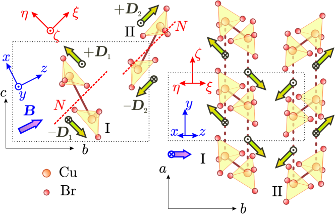
Figure 1: Geometry of DM vectors in BPCB, field (Latin) and crystal (Greek) related spin coordinate systems.

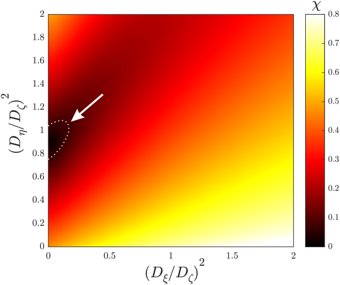
Figure 2: The criterion (54) plotted as function of $X$ and $Y$ [see definition (51)] for $K=0.8$. Region with $\chi\lesssim 0.1$ is highlighted on the plot.

Symmetry of BPCB allows the following DM vectors on each of the ladder types: $\mathbf{D}_{1}=(D_{\xi},D_{\eta},D_{\zeta})$ and $\mathbf{D}_{2}=(-D_{\eta},D_{\xi},D_{\zeta})$. Here $\zeta\parallel a$, $\xi\parallel N$, as shown in Fig. 1. Assuming that the prefactor ${A}$ is field direction independent, the gaps for $B\parallel N$ and $B\parallel b$ are:

$$\Delta_{N}^{(1)}={A}(D_{\eta}^{2}+D_{\zeta}^{2})^{\alpha/2}$$ (48)

$$\Delta_{N}^{(2)}={A}(D_{\xi}^{2}+D_{\zeta}^{2})^{\alpha/2}$$ (49)

$$\Delta_{b}={A}\Bigl{(}D_{\zeta}^{2}+\frac{(D_{\xi}+D_{\eta})^{2}}{2}\Bigr{)}^{\alpha/2},$$ (50)

where $\alpha=\frac{4K}{4K-1}$. In case of $B\parallel b$ the ladders are equivalent and there is just a single gap $\Delta_{b}$, while for $B\parallel N$ the gaps in the ladders I and II are $\Delta_{N}^{(1)}$ and $\Delta_{N}^{(2)}$.

It is convenient to introduce a simplified notation for the ratios of the gaps and DM vector components:

$$\frac{\Delta_{N}^{(1)}}{\Delta_{N}^{(2)}}=R_{12},~{}\frac{\Delta_{b}}{\Delta_{N}^{(2)}}=R_{b2},~{}\left(\frac{D_{\xi}}{D_{\zeta}}\right)^{2}=X,~{}\left(\frac{D_{\eta}}{D_{\zeta}}\right)^{2}=Y.$$ (51)

In this notation:

$$R_{12} =\left(\dfrac{1+Y}{1+X}\right)^{\alpha/2}$$ (52)

$$R_{b2} =\left(\dfrac{1+\frac{1}{2}\left(\sqrt{X}+\sqrt{Y}\right)^{2}}{1+X}\right)^{\alpha/2}$$ (53)

Relations (52) are the important consequence of ’solitonic’ excitation picture. They link the direction of DM vector in BPCB to the experimentally observed gap ratios.

For a given $K=0.8$ that follows from TLSL calculations we need to find the non-negative parameters $X$ and $Y$ that satisfy relations (52). Thus, one can say that we experimentally determine the orientation of DM vector. We can define the deviation as:

$$\chi=\sqrt{\left(\dfrac{R_{12}^{\mathrm{Obs}}-R_{12}^{\mathrm{Calc}}}{R_{12}^{\mathrm{Obs}}}\right)^{2}+\left(\dfrac{R_{b2}^{\mathrm{Obs}}-R_{b2}^{\mathrm{Calc}}}{R_{b2}^{\mathrm{Obs}}}\right)^{2}}$$ (54)

As Fig. 2 shows, for $K=0.8$ the experimental gap ratio is reproduced for $D_{\xi}\simeq 0$ and $D_{\eta}\simeq 0.9D_{\zeta}$. Found projections of DM vectors on $(bc)$ plane are the same as in Ref. Čižmár et al., 2010, but our analysis predicts that DM vector component parallel to the ladder has approximately the same length as the component transverse to the ladder. The resulting orientations of DM vectors in the ladders are shown in Fig. 1.

References

• Cabra et al. (1998) D. C. Cabra, A. Honecker, and P. Pujol, Magnetization plateaux in $n$-leg spin ladders, Phys. Rev. B 58, 6241 (1998).
• Giamarchi (2003) T. Giamarchi, Quantum Physics in One Dimension (Clarendon, Oxford, 2003).
• Kaplan (1983) T. A. Kaplan, Single-band Hubbard model with spin-orbit coupling, Z. Phys. B 49, 313 (1983).
• Shekhtman et al. (1992) L. Shekhtman, O. Entin-Wohlman, and A. Aharony, Moriya’s anisotropic superexchange interaction, frustration, and Dzyaloshinsky’s weak ferromagnetism, Phys. Rev. Lett. 69, 836 (1992).
• Shekhtman et al. (1993) L. Shekhtman, A. Aharony, and O. Entin-Wohlman, Bond-dependent symmetric and antisymmetric superexchange interactions in La2CuO4Phys. Rev. B 47, 174 (1993).
• Hikihara and Furusaki (2004) T. Hikihara and A. Furusaki, Correlation amplitudes for the spin-1/2 XXZ chain in a magnetic field, Phys. Rev. B 69, 064427 (2004).
• Zamolodchikov (1995) A. B. Zamolodchikov, Mass scale in the sine-Gordon model and its reduction, International Journal of Modern Physics A 10, 1125 (1995).
• Furuya and Momoi (2018) S. C. Furuya and T. Momoi, Electron spin resonance for the detection of long-range spin nematic order, Phys. Rev. B 97, 104411 (2018).
• Oshikawa and Affleck (2002) M. Oshikawa and I. Affleck, Electron spin resonance in $S=1/2$ antiferromagnetic chains, Phys. Rev. B 65, 134410 (2002).
• Ozerov et al. (2015) M. Ozerov, M. Maksymenko, J. Wosnitza, A. Honecker, C. P. Landee, M. M. Turnbull, S. C. Furuya, T. Giamarchi, and S. A. Zvyagin, Electron spin resonance modes in a strong-leg ladder in the Tomonaga-Luttinger liquid phase, Phys. Rev. B 92, 241113 (2015).
• Lukyanov and Zamolodchikov (2001) S. Lukyanov and A. Zamolodchikov, Form factors of soliton-creating operators in the sine-Gordon model, Nuclear Physics B 607, 437 (2001).
• Kuzmenko and Essler (2009) I. Kuzmenko and F. H. L. Essler, Dynamical correlations of the spin-1/2 Heisenberg XXZ chain in a staggered field, Phys. Rev. B 79, 024402 (2009).
• Furuya and Oshikawa (2012) S. C. Furuya and M. Oshikawa, Boundary resonances in $S=1/2$ antiferromagnetic chains under a staggered field, Phys. Rev. Lett. 109, 247603 (2012).
• Bouillot et al. (2011) P. Bouillot, C. Kollath, A. M. Läuchli, M. Zvonarev, B. Thielemann, C. Rüegg, E. Orignac, R. Citro, M. Klanjšek, C. Berthier, M. Horvatić, and T. Giamarchi, Statics and dynamics of weakly coupled antiferromagnetic spin-1/2 ladders in a magnetic field, Phys. Rev. B 83, 054407 (2011).
• Čižmár et al. (2010) E. Čižmár, M. Ozerov, J. Wosnitza, B. Thielemann, K. W. Krämer, C. Rüegg, O. Piovesana, M. Klanjšek, M. Horvatić, C. Berthier, and S. A. Zvyagin, Anisotropy of magnetic interactions in the spin-ladder compound (C5H12N)2CuBr4Phys. Rev. B 82, 054431 (2010).