Hop Sampling: A Simple Regularized Graph Learning for Non-Stationary Environments

Abstract.

Graph representation learning is gaining popularity in a wide range of applications, such as social networks analysis, computational biology, and recommender systems. However, different with positive results from many academic studies, applying graph neural networks (GNNs) in a real-world application is still challenging due to non-stationary environments. The underlying distribution of streaming data changes unexpectedly, resulting in different graph structures (a.k.a., concept drift). Therefore, it is essential to devise a robust graph learning technique so that the model does not overfit to the training graphs. In this work, we present Hop Sampling, a straightforward regularization method that can effectively prevent GNNs from overfitting. The hop sampling randomly selects the number of propagation steps rather than fixing it, and by doing so, it encourages the model to learn meaningful node representation for all intermediate propagation layers and to experience a variety of plausible graphs that are not in the training set. Particularly, we describe the use case of our method in recommender systems, a representative example of the real-world non-stationary case. We evaluated hop sampling on a large-scale real-world LINE dataset and conducted an online A/B/n test in LINE Coupon recommender systems of LINE Wallet Tab. Experimental results demonstrate that the proposed scheme improves the prediction accuracy of GNNs. We observed hop sampling provides 7.97 % and 16.93 % improvements for NDCG and MAP compared to non-regularized GNN models in our online service. Furthermore, models using hop sampling alleviate the oversmoothing issue in GNNs enabling a deeper model as well as more diversified representation.

1. Introduction

Figure 1. LINE Coupon Service. Everyday new coupons appear or disappear with sales events. User preference is heavily dependent on various factors such as discount ratio, and food type. We evaluate our graph learning method on such a non-stationary environment.

Graph is an widely-applicable data structure, e.g. knowledge graphs, social networks, bioinformatics, recommender systems, etc. (Angles and Gutierrez, 2008; Hamilton et al., 2017b). In recent years, graph neural networks (GNNs) (Scarselli et al., 2008) have recently been highlighted as a promising approach to handle graph-structured data, and have significantly improved diverse graph problems (Grover and Leskovec, 2016; Yu et al., 2017). GNNs are broadly based on the message-passing algorithms, where each entity aggregates the representation vectors from its neighbors, recursively. After $k$ aggregation steps, each node learns a new representation that is computed from the feature information of $k$-hop neighborhood as well as itself. Consequently, GNNs are capable of capturing the structural information in the underlying graphs (Xu et al., 2018a).

However, applying GNNs for real-world problems is not straightforward due to the following challenges. Primarily, real-world environments are usually non-stationary due to the evolving graph structures (a.k.a., concept drift). Consider a recommender system, for instance, new users and items appear everyday, and the interaction between them varies as the users’ item preferences change by external events (Xiang et al., 2010) (see Table 1). There often exists a time delay between the training and inference stages in many real-world services, the learning model would encounter unseen graphs in the online environment. As such, we have to develop a flexible graph learning scheme that does not overfit to specific graphs that appeared during the training dataset.

Secondly, stacking deep GNN layers is non-trivial task. In particular, Graph Convolutional Networks (GCNs) (Kipf and Welling, 2017), the most prominent GNN model, are known to deliver the best performance when it is composed of two or one layers owing to the oversmoothing problems (Kipf and Welling, 2017; Klicpera et al., 2018); it undermines the advantage of graph neural networks that can propagate node representations between arbitrary distant nodes. Such a problem becomes crucial in heterogeneous bipartite graphs that commonly emerges in real-world applications. Taking the e-commerce as an example, the two-hop propagation in the user-item interaction graph is, in fact, equivalent to the one-hop graph among users. Such shallow GNNs can not only lead to representation power degradation, but learn less distinct representation.

Recently, there have been several studies to address each of the presented challenges. To resolve the first challenge, graph regularization techniques mostly based on the node sampling scheme has been researched (Hamilton et al., 2017a; Huang et al., 2018; Chen et al., 2018; Chiang et al., 2019). On the other hand, to relieve the oversmoothing issue mentioned in the second challenge, variants of GNN with modifications on the propagation steps have been explored; APPNP (Klicpera et al., 2018) adopts the approximated personalized propagation scheme while JK-Nets (Xu et al., 2018b) uses dense connections between GNN blocks of multiple hops. Although suggested works could successfully resolve each challenge respectively in public datasets, we empirically found that those approachesLINE are not sufficient to fully handle non-stationary real-world datasets, as reported in Section 4.

In this paper, we propose Hop Sampling, which is a simple but effective regularization scheme that can improve the previous GNNs to learn better graph representation that is applicable even in a non-stationary environment. Hop sampling samples the number of aggregation/propagation steps during training stages rather than fixing it, unlike in most of the previous approaches. Moreover, we would like to stress that the presented work is a complementary technique that can be applied together with the existing approaches.

We evaluate the hop sampling on a large-scale real-world dataset collected from LINE Coupon service (see Figure 1), and run A/B/n test in our online services. The experimental results demonstrate that the suggested model increases the ranking accuracy and allows the representation to be diversified, i.e., personalized. We further found our model successfully avoid the oversmoothing issue even with the high number of propagation steps.

Table 1. Statics of Line Coupon Dataset. First two columns in the table represents the percentage of intersection and new appearances of node/edge between the user-item interaction graph of two consecutive days, respectively. Third column describes the coefficient of variation regarding to the number of node/edge. As illustrated in the table, new nodes and edges appear in large proportions everyday and the number of nodes, and edges varies considerably, showing the serious non-stationarity of the dataset.

	Intersection	New	Coefficient of Variation
Node	5.66 %	94.34 %	27.87 %
Edge	2.21 %	97.79 %	27.39 %

2. Preliminaries

2.1. Graph Convolutaional Networks

Consider a graph $G=(V,E)$ where $V$ and $E$ denotes nodes and edges, respectively. The adjacency matrix is defined as $A\in\mathbb{R}^{|V|\times|V|}$ of which the element $A_{i,j}$ is associated to the edge $(v_{i},v_{j})\in V$. To allow each node to gather its representation as well as its neighbors, the self loops are added to the adjacency matrix: $\tilde{A}=A+I$.

For given initial embedding matrix $X\in\mathbb{R}^{|V|\times D}$, graph convolutional network (GCN) updates the node representation by recursively aggregating embedding vectors of its neighbor: representations are propagated as following:

(1) $$Z^{(k)} =\sigma(\hat{A}Z^{(k-1)}W^{(k)})$$

(2) $$\hat{A} =\tilde{D}^{(-1/2)}\tilde{A}\tilde{D}^{(-1/2)}$$

where $Z^{(0)}=X$, $W^{(k)}$ is the learnable filter matrix of $k^{th}$ layer, $\sigma(\cdot)$ is the non-linear activation function (i.e., ReLU), and $\hat{A}$ is the symmetrically normalized adjacency matrix with self-loops with the diagonal degree matrix of $\tilde{A}$, $\tilde{D}$.

2.2. Approximate Personalized Propagation of Neural Predictions

Despite the noticeable progress, previous GCN based approaches commonly focused on the shallow networks due to the oversmoothing. Approximate personalized propagation of neural predictions (APPNP) (Klicpera et al., 2018) introduced a propagation scheme of personalized PageRank (Page et al., 1999) and relieved the issue. APPNP add a teleport term to the root node in the graph propagation step, allowing the model to gather information from a far neighborhood while preserving the locality:

(3) $$Z^{(k)} =(1-\alpha)\hat{A}Z^{(k-1)}+\alpha H$$

(4) $$=\tilde{A}_{k}H=\Big{(}(1-\alpha)^{k}\hat{A}^{k}+\alpha\sum_{i=0}^{k-1}(1-\alpha)^{i}\hat{A}^{i}\Big{)}H$$

where $Z^{(0)}=H=f_{p}(X)$ is the prediction matrix calculated by the neural network $f_{p}$ and $\alpha$ is the teleport probability. Note that, APPNP separates the prediction and propagation stage so that the model does not have learnable parameters during the propagation stage, which helps the model to avoid overfitting.

3. Proposed Method: Hop-Sampling

Previous studies, including GCN and APPNP, have focused on the dataset of which the graph is fixed between train and test set. As such, most GNN approaches are inherently transductive; they often fail to generalize for unseen graphs (Hamilton et al., 2017a). In the real-world applications, however, the environment is often non-stationary, therefore a robust inductive graph learning scheme that does not overfit to the train graphs is required. To tackle the issue, we propose a simple but effective regularization method, Hop Sampling: In the hop sampling scheme, we randomly select the number of propagation steps from $0$ to $K$ for every batch instead of fixing it. Consequently, the proposed scheme optimizes the expectation of embedding instead of the final embedding:

(5) $$\theta^{*}=\operatorname*{arg\,min}_{\theta}\sum_{t\in\mathcal{T}}l_{\theta}(Z=\mathbb{E}_{k\sim p_{samp}(\cdot)}\big{[}Z_{t}^{(k)}\big{]})$$

where $l_{\theta}$ is a loss function of learnable paramater $\theta$ in GNNs and embedding networks, and $p_{samp}$ is a sampling distribution. Note that our model is equivalent to the existing approaches when the sampling distribution is an indicator function: $\mathbbm{1}(k=K)$. In this paper, we adopted a discrete uniform distribution $\mathcal{U}(0,K)$ instead. Future work includes considering non-uniform parameterized sampling probability distribution (i.e., learn to select the hop). When validation and testing, we do not sample $k$.

Regularization Perspectives.    It is recently studied that the graph representations tend to crumble after multiple propagation steps, especially in GCN based approaches. We believe one of main factors in the problem is that existing approaches lacks the signal helping the model to learn meaningful representation on intermediate propagation stages. In the meantime, hop sampling prevents GNNs from overfitting to a specific hop number and allows the model to learn informative embeddings at every propagation step.

Graph Sampling Perspectives.    Remark that in the propagation scheme, we can consider $k$ as a factor transforming the adjacency matrix propagating the initial feature matrix $H$, from $\hat{A}$ to $\tilde{A}_{k}$ as illustrated in eq (4). In that sense, hop sampling can be regarded as a new graph sampling technique when it is applied to APPNP. Consequently, the model using hop sampling experiences $K$ times larger variety of graphs during the training stage, helping the model to adapt a non-stationary environment easily and avoid overfitting.

4. Experiment Results

Table 2. Hyperparameters.

Hyperparameters	Values
Teleport probability $(\alpha)$	0.3
Dimension of node embedding $z_{i}$ ($D$)	128
# of propagation $(K)$	[1, 2, 4, 8, 16]
Batch size	1024
Initial learning rate	$3e^{-6}$
$\beta_{1}$ of Adam	0.9
$\beta_{2}$ of Adam	0.999

To demonstrate the effectiveness of hop sampling in real-world non-stationary applications, this paper addresses the use case of recommender systems as one of the representative examples. Utilizing GNNs in recommender systems has been recently received attention because of its capability to model the relational structure between user and item (Berg et al., 2017; Ying et al., 2018; Wang et al., 2019; Kim et al., 2019; Shin et al., 2020). Consider a recommender system with $N_{u}$ users and $N_{i}$ items. Each user and item becomes a node in bipartite graph $G_{t}$, of which the nodes are connected if there is positive interaction (e.g., click or use) between the corresponding user and item during a period of time $t\in\mathcal{T}=\{T_{1},\cdots,T_{L}\}$. In most real-world cases, the graph $G_{t}$’s are heterogeneous because users and items have different types of side-information. For example, user nodes may contain demographic properties such as age and gender, while item nodes may have item categories and visual-linguistic contents. Denote the side information of users $Y_{u}\in\mathbb{R}^{N_{u}\times M_{u}}$ and side information of items $Y_{i}\in\mathbb{R}^{N_{i}\times M_{i}}$. Then, the node feature matrix $X$ of each node type is obtained by separated embedding networks $f_{u}$ and $f_{i}$:

(6) $$X=\left[f_{u}(Y_{u});f_{i}(Y_{i})\right]\in\mathbb{R}^{(N_{u}+N_{i})\times D}.$$

Starting from the node feature, GNN transforms the node representation into $Z_{t}$ through $K$ propagation steps using the graph $G_{t}$. The role of GNN is to improve the node representation of each root node by gathering information from its neighborhood and features of itself. As a consequence, each node embeddings in bipartite graph are mixed by neighborhood items and users. Finally, we predict the preference scores between user and item after $t$ by computing the inner-product between embeddings of them:

(7) $$p_{t,i,j}=sigmoid(z^{T}_{t,i}z_{t,j}),$$

where $z_{t,i}$ is i-th row vector of the final node representation matrix $Z_{t}$. The model parameters are optimized to minimize the cross-entropy loss between predicted score and true interaction label for all time periods via stochastic gradient descent algorithms.

4.1. Dataset

We use a dataset collected from a large-scale coupon recommendation system in LINE service as described. We constructed the bipartite graph consists of those 120,000 user and 517 item nodes connected when the user used the corresponding coupon. As side information, we used gender, age, mobile OS type, and interest information for users, while brand, discount information, test, and image features for items. For each attribute, the shallow multi layer perceptrons (MLPs) are used to make $n$-dimensional feature vector, and we aggregate them with sum operation to obtain feature matrix $X$. We split a dataset on daily basis: the first 14 days, the subsequent 3 days, and the last 3 days as a train, valid, and test set, respectively, i.e., ${\scriptstyle|\mathcal{T}_{train}|=14,~{}~{}|\mathcal{T}_{valid}|=3,~{}~{}|\mathcal{T}_{test}|=3}$. For each day, we construct bipartite graphs $G_{t}$ by using interactions in the previous 28 days. As expected, interactions in valid and test set are masked on the graph during the experiments.

4.2. Comparable models

To demonstrate the recommendation performance of the proposed method, we compared our model with following models:

• Deep Neural Networks (DNNs) is equivalent to 0-hop GNN model, i.e., $K$=0, and compared to show the effect of the graph propagation on the recommender system.

• GCN (Kipf and Welling, 2017) GCN is one of the most widely used graph neural networks in the literature. GCN filters out noises in the graph based on graph signal processing.

• Jumping Knowledge Networks (JK-GCN) (Xu et al., 2018b) concatenates GCN blocks of multiple hops. This method helps to alleviate oversmoothing with skip connections by adaptively adjust aggregation range of neighbor nodes. We denote this model as JK-GCN in this paper.

• APPNP (Klicpera et al., 2018) adopts propagation scheme described in Section 2.2. We fix the prediction function $f_{\theta}$ as identity function, since we already have learnable parameters in $f_{u}$ and $f_{i}$.

• APPNP-Hop Sampling (HS) is the proposed model which applies propagation scheme and hop sampling together. To further show the generalizability, we also report the performance of GCN model with hop sampling, GCN-HS.

We applied node sampling techniques for every GNN model for the scalable and inductive graph learning; we sampled 10240 users uniformly at random for each batch. For the fairness of the comparison, we adopted the same network architectures for $f_{u}$ and $f_{i}$. Important hyperparameters are summarized in Table 2. Experiments were performed on NAVER SMART Machine Learning platform (NSML) (Kim et al., 2018; Sung et al., 2017) using PyTorch (Paszke et al., 2019).

[ caption = Average values for ranking metrics of 20 runs on the LINE dataset. , label = tab:performance, doinside=]lcccc Models NDCG@10 MAP@10 HIT@10
DNN 0.1685 0.1337 0.3227
GCN 0.2114 0.1652 0.4214
JK-GCN 0.1583 0.1208 0.326
APPNP 0.2919 0.2344 0.5852
GCN-HS 0.2124 0.1685 0.4307
APPNP-HS 0.3039 0.2487 0.5922

[ caption = Average values for diversity metrics of 20 runs on the LINE dataset. , label = tab:diversity, doinside=]lcccc Models ILD@10 Coverage@10 Entropy@10
DNN 0.1441 0.0285 3.622
GCN 0.446 0.2923 4.733
JK-GCN 0.6288 0.4846 5.519
APPNP 0.7866 0.8434 6.629
GCN-HS 0.8536 0.9331 7.151
APPNP-HS 0.8229 0.8494 6.845

[ caption = Relative online performance improvement to Top Popular recommendation for ranking metrics in LINE Coupon recommender systems. , label = tab:online, doinside=]lcccc Models NDCG@10 MAP@10 HIT@10

APPNP 76.90 % 82.40 % 61.24 %
APPNP-HS 90.99 % 113.28 % 65.05 %

4.3. Experimental Results and Analysis

Primarily, we report three ranking metrics, Normalized Discounted Cumulative Gain (NDCG) (Järvelin and Kekäläinen, 2002), mean Average Precision (MAP), and Hit Ratio (HIT) to evaluate the ranking accuracy of the models. Since the optimal value for the number of propagation $K$ differs by the model, we chose models with the highest NDCG@10 value; the optimal $K$’s were 2 for GCN and JK-GCN, 4 for GCN-HS and APPNP-HS, and 8 for APPNP. As shown in Table LABEL:tab:performance, our models further enhances the prediction power for every ranking metric compared to GNN models only with node sampling.

Furthermore, we measured three diversity metrics, Inter-List Diversity (ILD) (Zhou et al., 2010), item coverage, and Shannon entropy for each model to show how diversified the recommended items are. As shown in Table LABEL:tab:diversity, our model shows the highest diversity values for every metric, which indicates that hop sampling relieves oversmoothing and encourages the model to learn graph representation in a more diversified way.

The prediction performance and recommendation diversity with different propagation steps are presented as well. Figure 2 and Figure 3 show that hop sampling enables the model to stack deeper layers for both GCN and APPNP whereas GCN and JK-GCN fail to learn graph representation over two hops as expected. As a result, both the prediction power and the diversity of hop sampling models are enhanced. Moreover, we found that hop sampling reduces variance of GNNs. Overall, APPNP-HS, with $K$=4 shows the best graph representation in our experiment.

Finally, we conducted a synthetic experiment to see the effect of hop-sampling in extremely non-stationary conditions. In real-world cases, we have experienced the situation that the empty user-interaction graph is given to our systems due to some practical issues such as log data omission. Similarly, we hypothetically remove edges of graphs in test datasets and compared the result between APPNP and APPNP with hop sampling. Figure 4 shows that APPNP without hop sampling suffer from the overfitting while the test accuracy continuously decreases over the train epochs. We believe the hop sampling helps the model not to rely on the training graph overly, and the initial embedding matrix $X$ is learned more robustly and adequately.

We have deployed best performing GNN models on offline test, APPNP and APPNP-HS, in LINE Coupon service and run A/B/n tests to evaluate the online performance on our LINE Coupon recommender systems in LINE Wallet Tab for four days. Relative performance improvement to non-personalized Top Popular recommendation is reported in Table LABEL:tab:online. As shown in results, GNNs provides significant improvement to our systems, and hop sampling further enhances the recommendation performance by 7.97 %, 16.93 %, and 2.37 % for NDCG, MAP, and HIT, respectively, compared to the APPNP with node sampling.

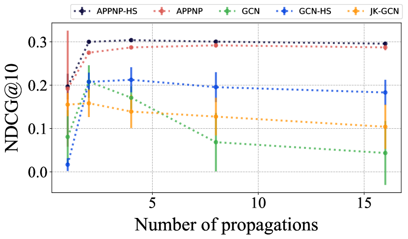
Figure 2. NDCG@10 by the number of propagation steps on a LINE dataset. Error bar indicates 95% confidence interval.

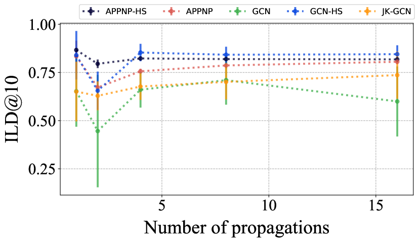
Figure 3. ILD@10 the number of propagation steps on a LINE dataset. Error bar indicates 95% confidence interval.

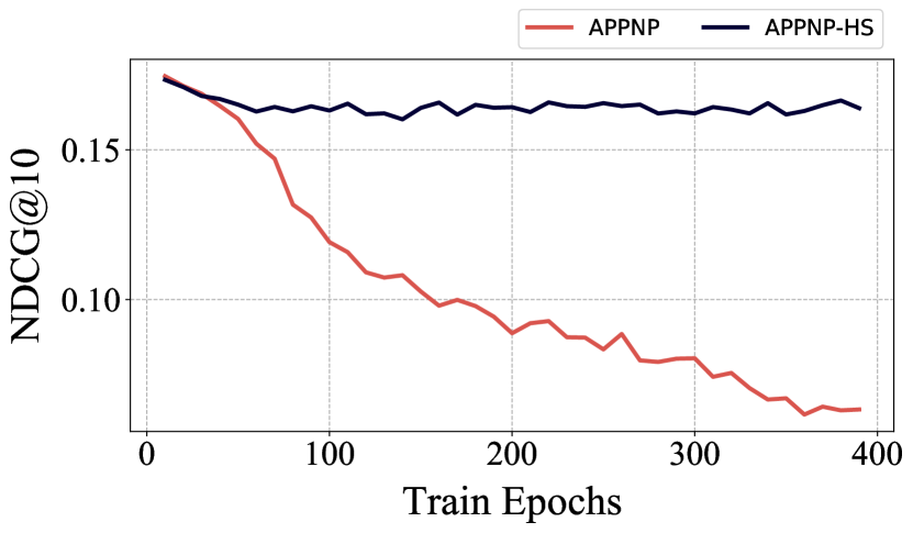
Figure 4. NDCG@10 by the train epochs on a LINE dataset with empty test graphs.

5. CONCLUSION

In this paper, we presented Hop Sampling, a novel and straightforward technique helping models to learn better graph representation. By varying the number of propagation steps randomly, hop sampling alleviates the overfitting and oversmoothing problems in GNNs. Experimental studies on real-world, large-scale LINE Coupon recommender system shows the proposed scheme improves the recommendation quality in terms of both ranking accuracy and recommendation diversity.

- (1)
- Angles and Gutierrez (2008) Renzo Angles and Claudio Gutierrez. 2008. Survey of graph database models. ACM Computing Surveys (CSUR) 40, 1 (2008), 1–39.
- Berg et al. (2017) Rianne van den Berg, Thomas N Kipf, and Max Welling. 2017. Graph convolutional matrix completion. arXiv preprint arXiv:1706.02263 (2017).
- Chen et al. (2018) Jie Chen, Tengfei Ma, and Cao Xiao. 2018. Fastgcn: fast learning with graph convolutional networks via importance sampling. In International Conference on Learning Representations (ICLR).
- Chiang et al. (2019) Wei-Lin Chiang, Xuanqing Liu, Si Si, Yang Li, Samy Bengio, and Cho-Jui Hsieh. 2019. Cluster-gcn: An efficient algorithm for training deep and large graph convolutional networks. In Proceedings of the 25th ACM SIGKDD International Conference on Knowledge Discovery & Data Mining. 257–266.
- Grover and Leskovec (2016) Aditya Grover and Jure Leskovec. 2016. node2vec: Scalable feature learning for networks. In Proceedings of the 22nd ACM SIGKDD international conference on Knowledge discovery and data mining. ACM, 855–864.
- Hamilton et al. (2017a) Will Hamilton, Zhitao Ying, and Jure Leskovec. 2017a. Inductive representation learning on large graphs. In Advances in Neural Information Processing Systems. 1024–1034.
- Hamilton et al. (2017b) William L Hamilton, Rex Ying, and Jure Leskovec. 2017b. Representation learning on graphs: Methods and applications. arXiv preprint arXiv:1709.05584 (2017).
- Huang et al. (2018) Wenbing Huang, Tong Zhang, Yu Rong, and Junzhou Huang. 2018. Adaptive sampling towards fast graph representation learning. In Advances in neural information processing systems. 4558–4567.
- Järvelin and Kekäläinen (2002) Kalervo Järvelin and Jaana Kekäläinen. 2002. Cumulated gain-based evaluation of IR techniques. ACM Transactions on Information Systems (TOIS) 20, 4 (2002), 422–446.
- Kim et al. (2018) Hanjoo Kim, Minkyu Kim, Dongjoo Seo, Jinwoong Kim, Heungseok Park, Soeun Park, Hyunwoo Jo, KyungHyun Kim, Youngil Yang, Youngkwan Kim, et al. 2018. NSML: Meet the MLaaS platform with a real-world case study. arXiv preprint arXiv:1810.09957 (2018).
- Kim et al. (2019) Kyung-Min Kim, Donghyun Kwak, Hanock Kwak, Young-Jin Park, Sangkwon Sim, Jae-Han Cho, Minkyu Kim, Jihun Kwon, Nako Sung, and Jung-Woo Ha. 2019. Tripartite Heterogeneous Graph Propagation for Large-scale Social Recommendation. arXiv preprint arXiv:1908.02569 (2019).
- Kipf and Welling (2017) Thomas N Kipf and Max Welling. 2017. Semi-supervised classification with graph convolutional networks. In International Conference on Learning Representations (ICLR).
- Klicpera et al. (2018) Johannes Klicpera, Aleksandar Bojchevski, and Stephan Günnemann. 2018. Predict then Propagate: Graph Neural Networks meet Personalized PageRank. In International Conference on Learning Representations (ICLR).
- Page et al. (1999) Lawrence Page, Sergey Brin, Rajeev Motwani, and Terry Winograd. 1999. The PageRank citation ranking: Bringing order to the web. Technical Report. Stanford InfoLab.
- Paszke et al. (2019) Adam Paszke, Sam Gross, Francisco Massa, Adam Lerer, James Bradbury, Gregory Chanan, Trevor Killeen, Zeming Lin, Natalia Gimelshein, Luca Antiga, Alban Desmaison, Andreas Kopf, Edward Yang, Zachary DeVito, Martin Raison, Alykhan Tejani, Sasank Chilamkurthy, Benoit Steiner, Lu Fang, Junjie Bai, and Soumith Chintala. 2019. PyTorch: An Imperative Style, High-Performance Deep Learning Library. In Advances in Neural Information Processing Systems 32, H. Wallach, H. Larochelle, A. Beygelzimer, F. d'Alché-Buc, E. Fox, and R. Garnett (Eds.). Curran Associates, Inc., 8024–8035. http://papers.neurips.cc/paper/9015-pytorch-an-imperative-style-high-performance-deep-learning-library.pdf
- Scarselli et al. (2008) Franco Scarselli, Marco Gori, Ah Chung Tsoi, Markus Hagenbuchner, and Gabriele Monfardini. 2008. The graph neural network model. IEEE Transactions on Neural Networks 20, 1 (2008), 61–80.
- Shin et al. (2020) Kyuyong Shin, Young-Jin Park, Kyung-Min Kim, and Sunyoung Kwon. 2020. Multi-Manifold Learning for Large-scale Targeted Advertising System. arXiv preprint arXiv:2007.02334 (2020).
- Sung et al. (2017) Nako Sung, Minkyu Kim, Hyunwoo Jo, Youngil Yang, Jingwoong Kim, Leonard Lausen, Youngkwan Kim, Gayoung Lee, Donghyun Kwak, Jung-Woo Ha, et al. 2017. Nsml: A machine learning platform that enables you to focus on your models. arXiv preprint arXiv:1712.05902 (2017).
- Wang et al. (2019) Hongwei Wang, Fuzheng Zhang, Mengdi Zhang, Jure Leskovec, Miao Zhao, Wenjie Li, and Zhongyuan Wang. 2019. Knowledge-aware graph neural networks with label smoothness regularization for recommender systems. In Proceedings of the 25th ACM SIGKDD International Conference on Knowledge Discovery & Data Mining. 968–977.
- Xiang et al. (2010) Liang Xiang, Quan Yuan, Shiwan Zhao, Li Chen, Xiatian Zhang, Qing Yang, and Jimeng Sun. 2010. Temporal recommendation on graphs via long-and short-term preference fusion. In Proceedings of the 16th ACM SIGKDD international conference on Knowledge discovery and data mining. 723–732.
- Xu et al. (2018a) Keyulu Xu, Weihua Hu, Jure Leskovec, and Stefanie Jegelka. 2018a. How powerful are graph neural networks? arXiv preprint arXiv:1810.00826 (2018).
- Xu et al. (2018b) Keyulu Xu, Chengtao Li, Yonglong Tian, Tomohiro Sonobe, Ken-ichi Kawarabayashi, and Stefanie Jegelka. 2018b. Representation learning on graphs with jumping knowledge networks. In Proceedings of the 35th International Conference on Machine Learning, ICML 2018, Stockholmsmässan, Stockholm, Sweden, July 10-15, 2018.
- Ying et al. (2018) Rex Ying, Ruining He, Kaifeng Chen, Pong Eksombatchai, William L Hamilton, and Jure Leskovec. 2018. Graph convolutional neural networks for web-scale recommender systems. In Proceedings of the 24th ACM SIGKDD International Conference on Knowledge Discovery & Data Mining. ACM, 974–983.
- Yu et al. (2017) Bing Yu, Haoteng Yin, and Zhanxing Zhu. 2017. Spatio-temporal graph convolutional networks: A deep learning framework for traffic forecasting. arXiv preprint arXiv:1709.04875 (2017).
- Zhou et al. (2010) Tao Zhou, Zoltán Kuscsik, Jian-Guo Liu, Matúš Medo, Joseph Rushton Wakeling, and Yi-Cheng Zhang. 2010. Solving the apparent diversity-accuracy dilemma of recommender systems. Proceedings of the National Academy of Sciences 107, 10 (2010), 4511–4515.