Revealing Choice Bracketing

Abstract.

In a decision problem comprised of multiple choices, a person may fail to take into account the interdependencies between their choices. To understand how people make decisions in such problems, we design a novel experiment and revealed preference tests that determine how each subject brackets their choices. In separate portfolio allocation under risk, social allocation, and induced-value function shopping experiments, we find that 40-43% of our subjects are consistent with narrow bracketing while 0-15% are consistent with broad bracketing. Adjusting for each model’s predictive precision, 74% of subjects are best described by narrow bracketing, 13% by broad bracketing, and 6% by intermediate cases.

JEL codes: D01, D90

Keywords: choice bracketing, individual decision-making, revealed preference, experiment.

Individuals face many interconnected decisions. Optimal decision-making involves integrating these choices into a comprehensive set of feasible combinations and selecting the best course of action, a procedure known as broad bracketing. Despite its normative appeal, broad bracketing often has counter-intuitive implications. For example, a broad bracketer who values fairness may sacrifice the immediate well-being of those around them to redistribute to more deserving individuals further away. Tversky & Kahneman, (1981) show that many people fail to bracket broadly and suggest that they instead make each decision in isolation without considering the relevant context, a procedure known as narrow bracketing.

How an individual perceives their problem significantly influences their decision-making process. Nearly every single behavioral model and most “rational” ones require some assumption about how people bracket choices. Nevertheless, systematic studies of bracketing are few and far between. No existing studies, including Tversky and Kahneman, can test both broad and narrow bracketing at the individual level, nor has the literature tested alternative models of non-narrow bracketing.

This paper provides the tools needed to reveal how individuals bracket their choices. To do so, we study a domain where each decision is composed of multiple parts but the payoff from a decision is determined by the sum of all items obtained from all parts. We propose intuitive yet rigorous revealed preference tests that disentangle a person’s preferences from how they bracket. We implement a novel experiment and apply our tests to reveal how each individual brackets. We find that most people bracket narrowly, but that a notable minority are broad bracketers.

In our setting, we can precisely define models of choice bracketing, and construct tests that differentiate between them. For example, a narrow bracketer behaves as if each part independently determines their payoff and maximizes a preference relation accordingly. To check for narrow bracketing, we perform a revealed preference test on a dataset of their choices, treating each part as an independent observation. Similarly, a broad bracketer acts as if they integrate all parts of the decision into a single feasible set and then maximizes a preference relation. To check for broad bracketing, we conduct a revealed preference test on a dataset that includes one choice and one feasible set per decision. These tests require minimal assumptions on the underlying preferences. Our approach extends to provide similar tests for an intermediate model of “partial-narrow” bracketing due to Barberis et al., (2006) and Rabin & Weizsäcker, (2009).

In our experiments, subjects make five decisions that each consist of either one or two parts. Every part is a budget set, and integrating the parts only requires addition. In two-part decisions, each good in the first part is a perfect substitute for a good in the second. Broad bracketers recognize and take full advantage of this substitutability, while narrow bracketers do not. Consequently, the two models make distinct predictions in every two-part decision.

We apply our design to portfolio choices among risky assets (Choi et al.,, 2007), social allocations between two anonymous other subjects (Andreoni & Miller,, 2002; Fisman et al.,, 2007), and shopping for goods with induced values over bundles. The Shopping Experiment allows us to conduct even more powerful tests of bracketing because preferences are known. Across the three experiments, 40-43% of subjects are consistent with narrow but not broad bracketing, 0-15% are consistent with broad but not narrow bracketing, and the remaining subjects are inconsistent with both models. We then determine which model best describes each subject’s bracketing based on both the number of errors they make relative to each model and the predictive precision of that model (Selten,, 1991). We classify 6-13% of subjects to broad bracketing, 68-78% to narrow bracketing, and only 3-9% to partial narrow bracketing, with variation across experiments.

Choice bracketing is tightly connected to the question of whether or not economic agents reap the benefits of specialization. Specialization, which requires boundary choices in our experiment, increases utility in the same way that comparative advantage increases total productivity in classic trade models. Economists have long recognized this connection, exemplified by Smith,’s (1776, p. 6) famous tale of the pin-making manufactory where 10 individuals “could make among them upwards of forty-eight thousand pins in a day…. But if they had all wrought separately and independently… they certainly could not each of them have made twenty.” Broad bracketers apply Smith’s insights to individual decision-making, while narrow bracketers fail to reap the gains from specialization. Our approach allows us to quantify the welfare losses from failure to specialize. For instance, in the Shopping Experiment, the subjects classified as narrow bracketers made an average of $1.34 less than the broad bracketers from the two-part decisions.

Because our tests are individual-level, they can provide evidence on why so many people bracket narrowly despite the gains from broad bracketing. In online follow-up experiments, we recorded choice process data and implemented a nudge to encourage subjects to “examine both parts” of the decision. While the nudge increased the proportion of subjects who looked at both parts, it had a limited effect on the rate of broad bracketing. In one arm of the Online Risk Experiment, we observed that about a quarter of the narrow bracketers had enough information to bracket broadly but did not do so. In the Online Shopping Experiment, a similar fraction used a calculator to compute the payoff of one or more bundles that were only feasible at the decision level and not in any part on its own. Both these behaviors indicate some consideration of how choices from both parts combine to determine payoffs. This suggests that not all narrow bracketing results from simply looking at one part of a decision at a time and making an optimal choice for that part on its own.

Bracketing also affects how one interprets behavior. A narrow bracketer’s reluctance to take a small yet actuarially favorable gamble indicates only slight risk aversion. However, for broad bracketers, the rejection of the same gamble signifies extreme risk aversion, given its minimal impact on their overall wealth (Rabin,, 2000). Our approach enables us to separate underlying preferences from bracketing, with implications for measuring risk or inequity aversion.

Failure to account for heterogeneity in bracketing can lead to misleading inferences. To illustrate, consider one part of one decision of the Social Experiment (Part 2 of Decision 1; see Table 2). On average, people make unequal allocations between the two anonymous others, dividing $16 into $6.80 and $9.20. This might suggest a lack of concern for equity, but paints a misleading picture. When we look only at the 75% of subjects classified as narrow bracketers, they on an average allocate $7.75 and $8.25 to each person. In contrast, the 10% classified as broad bracketers all allocate a $14 - $2 split but allocate $0 - $12 in the other part, achieving perfectly equal allocations at the decision level. After we take bracketing into account, these subjects all exhibit inequality averse behavior.

Most applications of prospect theory explicitly assume narrow bracketing (Camerer, 2004, Table 5.1; O’Donoghue & Sprenger,, 2018, Sections 3.4 and 4.5). Since it is impossible to avoid all other risks, a broad bracketer will not exhibit noticeable loss aversion over a moderate-stakes risk-taking opportunity (Barberis et al.,, 2006). At the same time, a form of broad bracketing is an equally crucial ingredient in other applications of prospect theory, for example, to casino gambling (Barberis,, 2012; Ebert & Strack,, 2015). Our results suggesting population-level heterogeneity in bracketing may reconcile the results rejecting broad bracketing (e.g. Tversky & Kahneman,, 1981) and those more supportive of it (e.g. Heimer et al.,, 2020 and Baillon et al.,, 2022).

Choice bracketing also plays a central role in understanding and modeling behavior in social decisions. For example, Sobel, (2005, p. 400) remarks that in experiments studying social decisions, a subject should “maximize her monetary payoff in the laboratory and then redistribute her earnings to deserving people later… if the concern for inequity was ‘broadly bracketed.”’ However, the literature he surveys and our analysis both find evidence consistent with subjects caring about narrowly-bracketed equity (e.g. Charness & Rabin,, 2002; Bolton & Ockenfels,, 2000) and inconsistent with such a form of broadly-bracketed equity.

Standard economic analyses make assumptions about bracketing as well. As noted by a recent graduate economics textbook, “Although choice bracketing has been largely ignored in economics, models in economic theory often implicitly assume and invoke it” (Dhami,, 2016, p. 1469). Many analyses exclude some related choices from the model (implicitly assuming a form of narrow bracketing) yet interpret results in terms of a fully rational choice. Our results suggesting that most people are narrow bracketers lend support to this approach, with the caveat that some subjects seem best modeled as broad bracketers.

1. Testing choice bracketing

We consider a decision-maker (DM) who faces $T$ decision problems involving alternatives contained in $\mathbb{R}_{+}^{n}$. Decision $t$ consists of $K_{t}\geq 1$ parts. Formally, the feasible set from part $k$ of decision $t$ is $B^{t,k}$, assumed to be compact. The DM chooses one alternative, denoted $x^{t,k}$, from each $B^{t,k}$. They face parts concurrently, and their payoff in decision $t$ depends only on the sum of their choices across parts of the decision,

$$x^{t}=\sum_{k=1}^{K_{t}}x^{t,k},$$

which we call the “final alternative”. A real world analogue consists of a scanner dataset with purchases at different stores (parts, indexed by $k$) in a given time period (a decision, indexed by $t$), and the shopper consumes these purchases after buying at all stores but before the next period.

In our first two models of bracketing, the DM is endowed with a complete, transitive, continuous, and monotone preference relation $\succsim$ over $\mathbb{R}_{+}^{n}$. A DM broadly brackets if they take the interaction between all the parts of the decision fully into account when making their choice. Concretely, a broad bracketer maximizes $\succsim$ over the feasible set of final alternatives for the decision problem,

$$B^{t}=\left\{\sum_{k=1}^{K_{t}}y^{t,k}:y^{t,k}\in B^{t,k}\right\}.$$

That is, a broad bracketer recognizes the underlying budget set defined by its parts, and their choices maximize $\succsim$ over the alternatives contained in it.

A number of experiments have documented that subjects fail to broadly bracket (e.g. Tversky & Kahneman,, 1981; Rabin & Weizsäcker,, 2009), and suggested that people instead narrowly bracket by maximizing their preferences within each part of the decision. Formally, a narrow bracketer chooses the alternative in part $k$ of decision $t$ that maximizes a fixed preference relation $\succsim$ over $B^{t,k}$. In words, they maximize their preferences part-by-part rather than decision-by-decision. A broad bracketer takes into account that good $i$ in part $k$ is a perfect substitute for good $i$ in part $k^{\prime}$, whereas a narrow bracketer does not consider any complementarities across parts of the decision.

We interpret each decision problem as being faced independently from and in the same set of economic circumstances as the others, and that the order of the parts does not matter. Thus, there are no complementarities across decision problems, only among parts within the same decision problem.

1.1. Predictions

How the DM brackets and their underlying preference relation are unobservable. We instead observe a finite sequence of choices from the $T$ decision problems

$$\mathcal{D}=\left\{\left(x^{t,k},B^{t,k}\right)\right\}_{(t,k)}$$

with $x^{t,k}$ denoting the alternative selected in part $k$ of decision $t$ and $x^{t}=\sum_{k^{\prime}=1}^{K_{t}}x^{t,k^{\prime}}$ the final alternative selected in decision $t$. In our experiments and the predictions below, we assume that each choice represents strict preference, though we could generalize all of our conditions to allow for indifference. Our theoretical results provide conditions necessary and sufficient for this dataset to be rationalized by one of the models of bracketing.

First, we clarify when data is consistent with a particular model of bracketing. The dataset $\mathcal{D}$ is rationalized by broad bracketing if there exists an increasing utility function $u:\mathbb{R}_{+}^{n}\rightarrow\mathbb{R}$ so that

$$x^{t}=\arg\max_{x\in B^{t}}u\left(x\right)$$

for every decision $t$. Similarly, the dataset $\mathcal{D}$ is rationalized by narrow bracketing if there exists an increasing $u:\mathbb{R}_{+}^{n}\rightarrow\mathbb{R}$ so that

$$x^{t,k}=\arg\max_{x\in B^{t,k}}u\left(x\right)$$

for every part $k$ and decision $t$.

Now, we provide necessary conditions for rationalization by a model of bracketing. The DM’s choice reveals their preference among a set of alternatives (determined by how they bracket) that may or may not equal their actual budget set. We use this observation to design direct tests of bracketing that compare choices in pairs of decisions or parts of decisions. To conduct a test of narrow bracketing, we compare a part of a first decision problem to the exact same choice set when it is a part of another decision (for example, as its own standalone decision). To conduct a test of broad bracketing, we compare two decisions for which the feasible aggregate alternatives overlap. We formalize the above predictions as follows.

Prediction 1 (NB-WARP).

Suppose that $\mathcal{D}$ is rationalized by narrow bracketing.
If $\left(x^{t,k},B^{t,k}\right),\left(x^{t^{\prime},k^{\prime}},B^{t^{\prime},k^{\prime}}\right)\in\mathcal{D}$ and $x^{t^{\prime},k^{\prime}}\in B^{t,k}\subseteq B^{t^{\prime},k^{\prime}}$, then $x^{t,k}=x^{t^{\prime},k^{\prime}}$.

Prediction 2 (BB-WARP).

Suppose that $\mathcal{D}$ is rationalized by broad bracketing.
For decisions $t,t^{\prime}$ in $\mathcal{D}$, if $x^{t^{\prime}}\in B^{t}\subseteq B^{t^{\prime}}$, then $x^{t}=x^{t^{\prime}}$.

These two predictions reflect the manifestations of the Weak Axiom of Revealed Preference (WARP) combined with each form of bracketing in our setting. Narrow bracketing requires that WARP holds when comparing any pair of parts of decisions, even when they belong to economically different decisions. Broad bracketing implies that WARP holds at the decision level, comparing final bundles that are feasible in both aggregate budget sets.

The next prediction reflects the appropriate manifestation of monotonicity in our setting.

Prediction 3 (BB-Mon).

Suppose that $\mathcal{D}$ is rationalized by broad bracketing.
For any decision $t$ in $\mathcal{D}$ and any $y\in B^{t}$, if $y\geq x^{t}$, then $y=x^{t}$.

BB-Mon requires that the subject chooses on the frontier of their aggregate budget set in a given decision. For a decision with two Walrasian budget sets with different price ratios, BB-Mon implies that the DM makes an extreme allocation in at least one of the budgets. In the part where good $i$ is relatively cheaper, they must exhaust the budget on good $i$, or consume none of good $i$ in the other part. Otherwise, they forgo the opportunity to consume more of each good.

1.2. Characterization

The above predictions are necessary but not sufficient conditions for the various types of bracketing. We obtain tight characterizations by extending the logic of the above to include indirect implications, in the same manner that Strong Axiom of Revealed Preference (SARP) extends WARP. Theorem 1 shows that these are necessary and sufficient conditions for a given dataset to be consistent with a particular form of bracketing.

Our tests are based on the classical SARP condition. Bundle $x$ is directly revealed preferred to $y$ in a dataset $\mathcal{D}$ consisting of single-part decisions, written $xP^{\mathcal{D}}y$, if either $x\geq y$ and $x\neq y$ or there exists $\left(x,B\right)\in\mathcal{D}$ so that $y\in B\backslash\{x\}$. The dataset $\mathcal{D}$ satisfies SARP if the binary relation $P^{\mathcal{D}}$ is acyclic.

Broad bracketing implies that the DM maximizes their underlying preferences over $B^{t}$. To test it, we apply SARP to the ancillary dataset

$$\mathcal{D}^{BB}=\left\{\left(x^{t},B^{t}\right)\right\}_{t\in T}.$$

We note that $B^{t}$ typically has a piece-wise linear budget-line even if each $B^{t,k}$ is a standard budget set.

Similarly, narrow bracketing implies that the DM maximizes an underlying preference on $B^{t,k}$ rather than $B^{t}$. As above, we test it by applying SARP to the ancillary dataset

$$\mathcal{D}^{NB}=\left\{\left(x^{s},B^{s}\right)\right\}_{s=1}^{\sum_{t=1}^{T}K_{t}}$$

where for each part $(t,k)$, there exists a unique $s$ so that $\left(x^{s},B^{s}\right)=\left(x^{t,k},B^{t,k}\right)$. That is, each part of every decision is treated as a separate, independent observation.

Theorem 1 formally states that applying SARP to the datasets $\mathcal{D}^{BB}$ and $\mathcal{D}^{NB}$ capture the complete implications of broad and narrow bracketing.

Theorem 1.

The following are true:
(i) The dataset $\mathcal{D}^{BB}$ satisfies SARP if and only if $\mathcal{D}$ is rationalizable by broad bracketing, and
(ii) The dataset $\mathcal{D}^{NB}$ satisfies SARP if and only if $\mathcal{D}$ is rationalizable by narrow bracketing.

Theorem 1 provides standard, albeit indirect, tests for broad and narrow bracketing. These conditions are readily applied and make only minimal restrictions on preferences. One can make tighter predictions by imposing more structure on the utility function that rationalizes the data. For instance, we impose that preferences are symmetric when we apply these tests to our experiments, which enables stronger versions of our SARP tests.

1.3. Partial-narrow bracketing

We also consider an intermediate model of bracketing lying between the two extremes, called $\alpha$-partial-narrow bracketing (PNB). Inspired by Barberis et al., (2006), Barberis & Huang, (2009), and Rabin & Weizsäcker, (2009), when choosing in part $k$ of decision $t$, the DM takes into account their choices in the other parts on utility, but only partially. Formally, dataset $\mathcal{D}$ is rationalized by $\alpha$-partial-narrow bracketing if

(1) $$\left(x^{t,1},\dots,x^{t,K_{t}}\right)=\arg\max_{y^{t,k}\in B^{t,k}\ \forall k}\alpha\sum_{k=1}^{K^{t}}u\left(y^{t,k}\right)+\left(1-\alpha\right)u\left(\sum_{k=1}^{K^{t}}y^{t,k}\right)$$

for all $t$. A PNB DM’s choice in part $k$ maximizes a utility that depends both on the final alternative and the one resulting from the part in isolation. They act as if they make a single choice in decision $t$ of an element of $\mathbb{R}_{+}^{nK_{t}}$, but they maximize a utility function derived from $u$ rather than $u$ itself. In contrast, a broad bracketer acts as if they choose a single element of $\mathbb{R}_{+}^{n}$, and a narrow bracketer as if they make $K_{t}$ independent choices of elements of $\mathbb{R}_{+}^{n}$. Recent models by Vorjohann, (2020) and Zhang, (2023) have this feature as well, but with different utilities over $\mathbb{R}_{+}^{nK_{t}}$ than Equation (1). They capture departures from broad bracketing by either substituing in a reference point for other parts or by imposing separability where $u$ is inseparable.

Psychologically, PNB captures a DM who thinks about their choice in the other parts, but not too much. A PNB DM views the same good in different parts as imperfect substitutes for each other. In contrast, a broad bracketer views them as perfect substitutes, and a narrow bracketer does not realize that they can substitute between them at all. A lower $\alpha$ indicates that they think more about the other parts. This leads a PNB DM to evaluate trade-offs between different goods in the same part differently than a narrow bracketer or broad bracketer would: they act as if their marginal rate of substitution between goods in part $k$ lies in between that of a narrow bracketer and that of a broad bracketer.

We also consider a related intermediate model of bracketing, “PNB-Personal Equilibrium (PNB-PE).” Formally,

$$x^{t,k}=\underset{y^{t,k}\in B^{t,k}}{\arg\max}\left[\alpha u\left(y^{t,k}\right)+(1-\alpha)u\left(\underset{k^{\prime}\in\left\{1\leq k^{\prime}\leq K^{t}:k^{\prime}\neq k\right\}}{\sum}x^{t,k^{\prime}}+y^{t,k}\right)\right].$$

for every part $k$ of decision $t$. While the functional form is similar to PNB, the DM acts as if they make $K_{t}$ independent choices of elements of $\mathbb{R}_{+}^{n}$, as a narrow bracketer would would. Their choices are the personal equilibrium (PE) of an intrapersonal game (Kőszegi & Rabin,, 2006; Lian,, 2019). A PNB-PE DM only considers the utility effect of $x^{t,-k}$ when choosing $x^{t,k}$, ignoring that they could change $x^{t,-k}$ in response to their choice. In contrast, PNB and the models in Vorjohann, (2020) and Zhang, (2023) assume the vector of choices maximizes a utility function on (the analog of) $\mathbb{R}_{+}^{nK_{t}}$ . Choices that satisfy Equation (1) are a personal equilibrium, and yield the highest utility even at the part-by-part level.

Theorem 2.

There exists an algorithm that outputs 1 if and only if $\mathcal{D}$ is rationalizable by $\alpha$-partial-narrow bracketing.

The algorithm that tests $\alpha$-partial-narrow bracketing is described in Appendix A. It reduces the problem of determining whether $\mathcal{D}$ is consistent with $\alpha$-partial-narrow bracketing to that of a standard linear programming problem. It runs in polynomial time with a fixed set of possible outcomes of each decision and its parts. We elaborate on the ideas behind the partial-narrow test below, and provide a formal proof in Appendix A.

The algorithm takes advantage of the formal similarity between Equation (1) and expected utility. Specifically, an $\alpha-$PNB DM with utility $u$ chooses $x^{t,1}$ in part 1 and $x^{t,2}$ in part 2 if and only if an expected utility DM with Bernoulli index $u$ chooses $\left(\psi\alpha,x^{t,1};\psi\alpha,x^{t,2};\psi(1-\alpha),x^{t}\right)$ from the menu of lotteries $\left\{\left(\psi\alpha,y^{1};\psi\alpha,y^{2};\psi(1-\alpha),y^{1}+y^{2}\right):y^{1}\in B^{t,1}\ \&\ y^{2}\in B^{t,2}\right\}$ where $\psi=(1+\alpha)^{-1}$. The algorithm first transforms the original dataset to an ancillary dataset where each decision is a single choice from a menu of lotteries. Each lottery in the menu is structured so that an alternative in part $k$ occurs with probability proportional to $\alpha$ for each part $k$ and their sum occurs with probability proportional to $(1-\alpha)$, and the DM’s choice is the lottery over their choices in each part and their sum. Existing results, e.g. (Clark,, 1993), provide necessary and sufficient conditions for the ancillary dataset to be rationalizable by expected utility. We show that whether or not it can be rationalized can be determined by examining the solution to a linear program.

2. Existing Evidence on Bracketing

The models we consider capture different forms of what Read et al., (1999) call choice bracketing: how an individual groups “individual choices together into sets.” Three main strands of evidence motivate explicit modeling of bracketing. First, people choose differently when a decision is framed as having multiple parts and when it is framed as a single choice. Second, subjects choose differently when the experimenter explicitly integrates a fixed alternative, e.g. an endowment of money, into the choice set as presented to them than when the subjects must integrate the same alternative themselves. Third, individuals assign dimensions of alternatives to different categories and do no treat the categories as fungible. We discuss these bodies of evidence in turn and then relate to our approach to choice bracketing. We first address the static, concurrent decisions to which our setting directly applies before turning to the important case of dynamic, or temporal, bracketing.

Most existing direct evidence of non-broad choice bracketing is derived from Tversky & Kahneman, (1981), in which subjects face the decision problem described in Table 1.

Table 1. Tversky and Kahneman’s Decision problem

Imagine that you face the following pair of concurrent decisions. First, examine both decisions, then indicate the options you prefer.
Decision (i). Choose between:

A. a sure gain of $240 [85%]

B. 25% chance to gain $1000,

and 75% chance to gain nothing [16%]

Decision (ii). Choose between:

C. a sure loss of $750 [13%]

D. 75% chance to lose $1000,

and 25% chance to lose nothing [87%]

This design can rule out broad bracketing and does so for the 73% of their subjects who choose A and D, which generates a first-order stochastically-dominated distribution over outcomes compared to the pair of choices B and C. It cannot falsify narrow bracketing since any pattern of choices except A and D is consistent with expected utility under either narrow or broad bracketing. Without further restrictions, their results are uninformative about the choice bracketing of subjects who do not choose A and D. Yet most subjects (72% and 68%) make other choices when Rabin & Weizsäcker, (2009) and Koch & Nafziger, (2019) revisit this design with incentivized choices. Other designs use assumptions on, or features of, preferences to measure bracketing. For example, Baillon et al., (2022) use the interaction between ambiguity and a random incentives scheme to estimate how ambiguity-averse subjects bracket. While their results suggest that about half of the ambiguity-averse subjects in their experiment bracketed narrowly, they do not speak to how the others bracketed. In contrast, our design enables us to falsify each of narrow and broad bracketing without parametric assumptions on utility. This design innovation enables us to provide direct estimates of heterogeneity in bracketing without parametric restrictions.

Other, less direct, evidence includes Samuelson’s (1963) report of a colleague who after declining a bet said that “I’ll take you on if you promise to let me make 100 such bets.” Under expected utility, if the colleague declined the bet for all wealth levels, then they should also decline all 100 bets at once. Related “calibration” results by Rabin, (2000), Safra & Segal, (2008), and Mu et al., (2020) suggest that evidence for small-stakes risk aversion but not excessively risk-averse behavior over larger stakes can be reconciled by not fully integrating such risks.

This evidence fits directly into our setting and motivates our work. For example, the Tversky & Kahneman, (1981) experiment is a single-decision dataset with $B^{1,1}=\{A,B\}$ and $B^{1,2}=\{C,D\}$. The choices $(A,D)$ violate BB-Mon and BB-SARP. Since no pair of choices can violate NB-SARP, our results show that their data cannot falsify narrow bracketing. This fact motivates our experimental design totest forms of non-broad bracketing, including narrow and partial-narrow.

A related set of experiments considers how an exogenously fixed quantity, like a monetary endowment, an asset, or a background risk, affects a person’s choice when separated from the description of available alternatives. Kahneman & Tversky, (1979, Problems 11-12) find that, when subjects are asked to imagine themselves endowed with experimental income and then given a hypothetical choice between two prospects, the modal choice varies if some of the endowment is instead explicitly incorporated into the prizes of available lotteries to create an economically-identical choice problem. Classic work by Yaari & Bar-Hillel, (1984) argues that people focus on equating gains across individuals rather than maximizing welfare. Recent work by Exley & Kessler, (2018) arrives at a stronger finding in a social allocation task: respondents tend to allocate equal numbers of money-valued tokens from a given account between two anonymous others, regardless of their initial endowments.

Within our framework, this second set of evidence corresponds to the special case where all but one of the parts are singleton menus. In that case, the singleton menus represent the endowments, and the non-singleton part the active choice. Representing the data in such a way, someone is consistent with narrow (or broad) endowment bracketing if and only if their choices satisfy NB- (or BB-) SARP.

The final body of evidence shows how failures of fungibility affect choice, overviewed by e.g. Thaler, (1999). Studies of the “flypaper effect” suggest that transfers earmarked for a particular type of spending tend to actually be spent there (Hines & Thaler,, 1995; Abeler & Marklein,, 2017). Empirical evidence from consumption choices after unexpected price changes support the lack of fungibility (Hastings & Shapiro,, 2013, 2018).

This evidence has a more complicated relationship with our setting. Thaler, (1985, 1999) and others (Galperti,, 2019; Kőszegi & Matějka,, 2020) explain the evidence through mental accounting (or budgeting): a person breaks up their overall budget by imposing category-specific budget constraints and optimizes within these constraints. The subject breaks up the overall decision into smaller parts. In contrast, a narrow choice bracketer fails to aggregate smaller parts into a single decision. Nevertheless, the two are not mutually exclusive, and how an agent brackets determines the category-specific budgets. On the one hand, if categories and parts coincide, then our model of narrow choice bracketing provides an extreme model of mental accounting. On the other hand, there is no reason to expect they should. As noted by (Thaler,, 1999, p. 184), “Accounts can be balanced daily, weekly, yearly, and so on, and can be defined narrowly or broadly,” so mental accounting is consistent with either broadly-bracketing across parts (Thaler,, 1985, p 207) or with narrowly bracketing each part (e.g. as described by Corollary 1 of Kőszegi & Matějka,, 2020). In the former case, the whole decision problem determines the category-specific budget, while in the latter, each part determines its own budget. As an example of how bracketing affects budgeting, Read et al., (1999) report that framing an equivalent choice in weeks or in months, analogous to combining parts, affects behavior. One can extend our framework by replacing the “SARP” part of NB- or BB- SARP with a revealed preference test for mental accounting, such as that of Blow & Crawford, (2018). Then, we have two joint tests: one for mental accounting where the budgets for each category are determined part-by-part, and one for mental accounting where the budgets for each category are determined at the decision-level.

Additional evidence for non-broad choice and endowment bracketing occurs in dynamic settings. Gneezy & Potters, (1997) show that subjects invest less in a risky asset when decisions are made and returns are shown period-by-period than when they must make their investment choices for the next three periods in advance. Thaler et al., (1997) show that subjects’ investment decisions varied systematically with the frequency with which they could revise their portfolio. In the field of finance, Shefrin & Statman, (1985) and Odean, (1998) document that people are more prone to sell stocks that have increased in value than those that have decreased (the disposition effect). Relatedly, Thaler & Johnson, (1990) show that people are more willing to take risk when investing gains from previous investments. Imas, (2016) provides evidence consistent with relatively more broad bracketing of paper losses from past gambles together with a current decision (as in the direction of Thaler & Johnson,’s (1990) “house money effect”), but relatively more narrow bracketing when past losses have been realized. Motivated by theoretical work applying cumulative prospect theory with broad bracketing to a sequence of risk-taking choices (Barberis,, 2012; Ebert & Strack,, 2015), recent evidence from Heimer et al., (2020) suggests that some subjects behave as if they do not narrowly bracket future risk-taking opportunities when making a current risk-taking decision.

Our approach can, in principle, be generalized to a dynamic setting. However, two key complications arise. First, the setting should comprise decision trees rather than sets of alternatives. This can be easily dealt with at the cost of additional notation. Second, issues of dynamic consistency and, in the presence of dynamic inconsistency, sophistication about future behavior arise. Our approach of comparing behavior when facing a broadly-presented decision (in this case, a set of complete contingent plans) with that when facing a comparable decision tree applies only under dynamic consistency. A new approach seems necessary with dynamically inconsistent behavior. We leave such an approach for future work.

We note here that there are even more ways to fail to broadly bracket in a dynamic setting. For instance, an agent may only look backwards, in that they take into account the results of their past decisions but neglect to consider how their current decision interacts with their future ones, or only look forwards, in that they take into account future interactions but not past results. Even more combinations are possible: they could look neither forwards nor backwards, or only look forwards a certain number of periods.

3. Experimental Design

We design and conduct three experiments to test the models of bracketing in different domains of choice. In each experiment, a participant faces five decision rounds, each consisting of one or two parts. Each part consists of all feasible integer-valued bundles of two goods obtained from a linear (or in one case, a piece-wise linear) budget set. At the end of the experiment, exactly one round is randomly selected for payment, which we call the “round that counts”. We sum all goods purchased in all parts of the decision in the round that counts to obtain the final bundle that determines payments. By design, there are no complementarities across decisions. We implement this experimental design to study choice bracketing in three domains of interest: portfolio choice under risk (Risk), a social allocation task (Social), and a consumer choice experiment in which we induced subjects’ values (Shopping).

In the Risk Experiment, each part of every decision asks the subject to choose an integer allocation of tokens between two assets. Each asset pays off on only one of two equally likely states: Asset A (or C) pays out only on a die roll of 1-3 whereas Asset B (or D) pays out only on a die roll of 4-6. The payoff of each asset varies across decision problems and across parts. Because each decision problem uses assets with two equally likely states, preferences over portfolios of monetary payoffs for each state should be symmetric across states.

In the Social Experiment, each part of every decision asks the subject to choose an integer allocation of tokens between two anonymous other subjects, Person A and Person B. The value of each token to A and B varies across decision problems and across parts. Because the two recipients are anonymous, we expect preferences to be symmetric across money allocated to A versus B.

In the Shopping Experiment, each part of every decision asks the subject to choose a bundle of integer quantities of fictitious “apples” and “oranges” subject to a budget constraint. The monetary payment for the experiment is calculated from the final bundle in the round that counts according to the function $\$\text{pay}=\frac{2}{5}\left(\sqrt{\text{\#apples}}+\sqrt{\text{\#oranges}}\right)^{2}$. This function induces payoffs that are symmetric in apples and oranges and that are strictly variety-seeking. Any subject who prefers more money to less will wish to maximize this payoff function regardless of their underlying utility function.

		Risk			Social			Shopping
Decision	Part	$I$	Asset A/C	Asset B/D	$I$	$V_{A}$	$V_{B}$	$I$	$p_{a}$	$p_{o}$
D1	1	10	$(\$1,\$0)$	$(\$0,\$1.20)$	10	$1	$1.20	8	2	1
	2	16	$(\$1,\$0)$	$(\$0,\$1)$	16	$1	$1	24	2	2
D2	1	14	$(\$2,\$0)$	$(\$0,\$2)$	14	$2	$2	32	2	1 (for 1st 8), 2
D3	1	10	$(\$1,\$0)$	$(\$0,\$1)$	10	$1	$1	30	3	3
	2	10	$(\$1,\$0)$	$(\$0,\$1.20)$	10	$1	$1.20	24	3	2
D4	1	16	$(\$1,\$0)$	$(\$0,\$1)$	16	$1	$1	12	1	1
D5	1	10	$(\$1,\$0)$	$(\$0,\$1.20)$	10	$1	$1.20	48	6	4
		$I$: income for a part (in tokens)
		$(\$x,\$y)$ indicates one			$V_{A}$: value/token to A			$p_{a}$: price/apple
		unit of asset pays $x/$y			$V_{B}$: value/token to B			$p_{o}$: price/orange
		if the die roll is 1-3/4-6

Table 2. Experimental Tasks

Our experimental budget sets, summarized in Table 2, allow us to conduct our revealed preference tests in the Risk and Social Experiments, and to conduct analogous tests that make use of the induced value function in our Shopping Experiment. Throughout, we refer to part $k$ of decision $t$ as Dt.k, or Dt if a round has only one part. The order of decisions and parts was varied across sessions (TSee nline Supplement).

We implemented our experiments on paper and followed up with some robustness treatments online (See Online Supplement). In each session, paper instructions were provided and read aloud, subjects were given the opportunity to ask questions privately, and then participants completed a brief comprehension quiz and the experimenter individually checked answers and explained any errors. The comprehension quiz had each subject calculate how payment would be determined from their allocations when a decision involves two parts. This was designed to ensure that each subject was aware of how to calculate payments in these cases, but without instructing them to consider all possible combinations of allocations across parts.

Each decision had a cover page indicating the number of parts in the decision, with each part stapled beneath as a separate page. Thus, a subject was always informed when a decision contained multiple parts, but could choose whether or not to look at both parts before making allocations. A subject indicated each allocation by highlighting the line corresponding to their choice for each part using a provided highlighter. Subjects were allowed no other aids at their desk when making choices. Only one decision was handed out to a subject at a time, and that decision was collected before the next round was handed out. The order of decisions, and of parts within each decision, was varied across sessions to allow us to test and control for order effects.

Sessions took place in two experimental economics labs in Canada from June 2019 to February 2020, each taking place in a one hour block. Subjects were recruited from the labs’ student participant pools to participate in one of the three experiments. Instructions, experimental materials, and details of the experimental procedure are provided in Online Supplement.

4. Results

This section reports the results of our experimental tests of the models of bracketing. For each test, we also compute results allowing for one or two “errors” relative to its requirements. We define an error as how far we would need to move a subject’s allocations for them to pass that test, measured in lines on the decision sheet(s). For instance, in Risk and Social, a subject is within one error of passing a test if revising the choice by shifting one token from one asset/person to the other in a single part would lead to choices that pass that test. They are within two errors of passing a test if shifting two tokens from one asset/person to the other, either in the same part or in different parts, would lead to choices that pass. For predictions that require Walrasian budget sets, we modify the tests to account for discreteness in our experiment.

4.1. Risk Experiment: How subjects behave

Consider Decision 1 in the Risk Experiment. Since Asset B in the first part is a perfect substitute for Asset D in the second, comparative advantage requires that the subject first purchases it in the part where it has a lower opportunity cost. Consequently, a broad bracketer necessarily allocates all of their wealth in the first part to Asset B before they allocate any to Asset D in the second (as required by BB-Mon). If preferences are symmetric across the two equally-likely states, then broad bracketing further requires that $x_{A}^{1,1}=0$. With risk aversion, broad bracketing makes even stronger predictions. The allocation $x_{A}^{1,1}=0$ and $x_{C}^{1,2}=14$ obtains a risk-free return of $14, and any other feasible allocation results in a first- or second-order stochastically dominated distribution over returns at the decision-level. In contrast, a narrow bracketer facing Decision 1 allocates at least half of their budget to Asset B in Part 1. If they are also risk-averse, then they allocate exactly half their budget in Part 2 to each asset.

Figure 1. Allocations in Risk

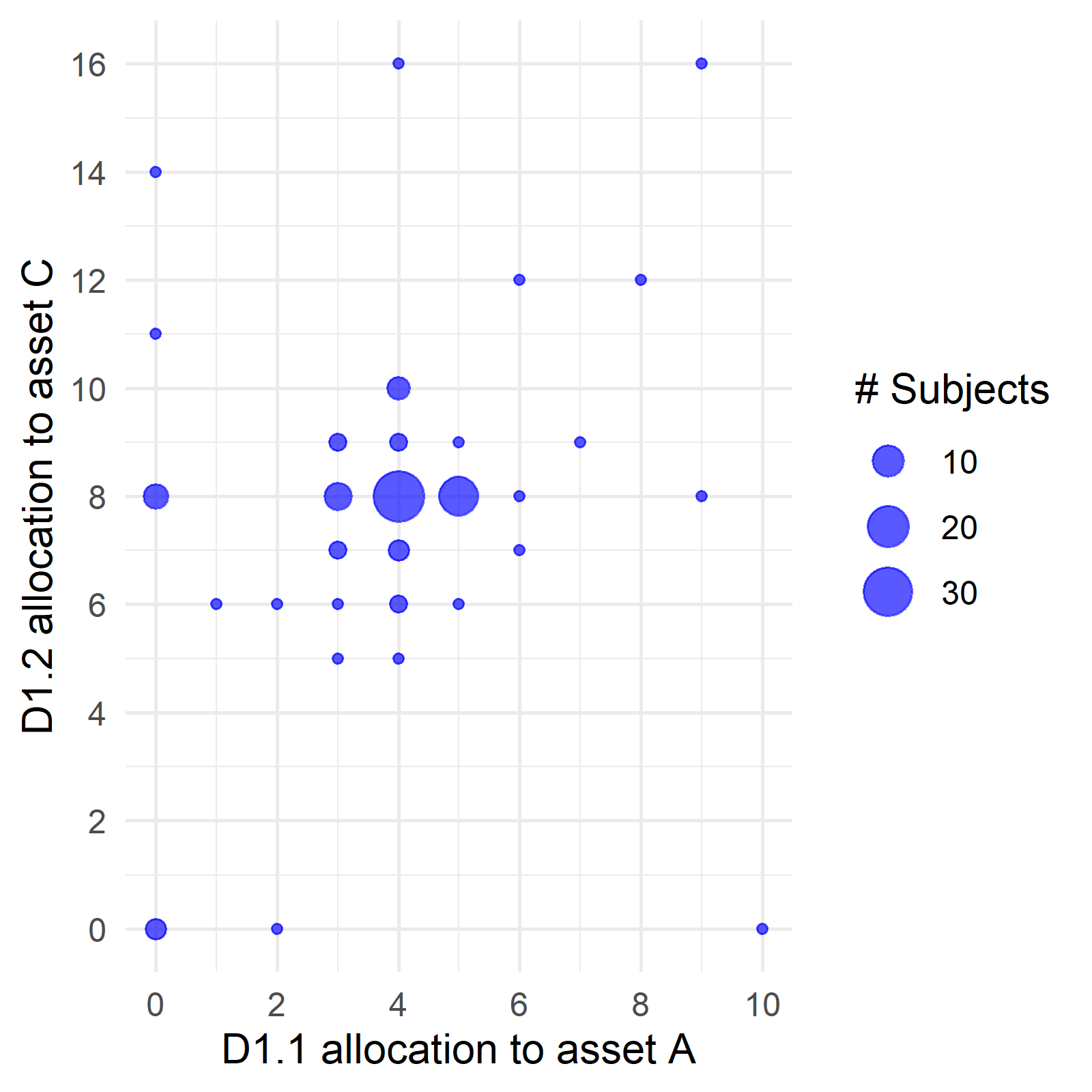
(a) D1 Allocation in Risk

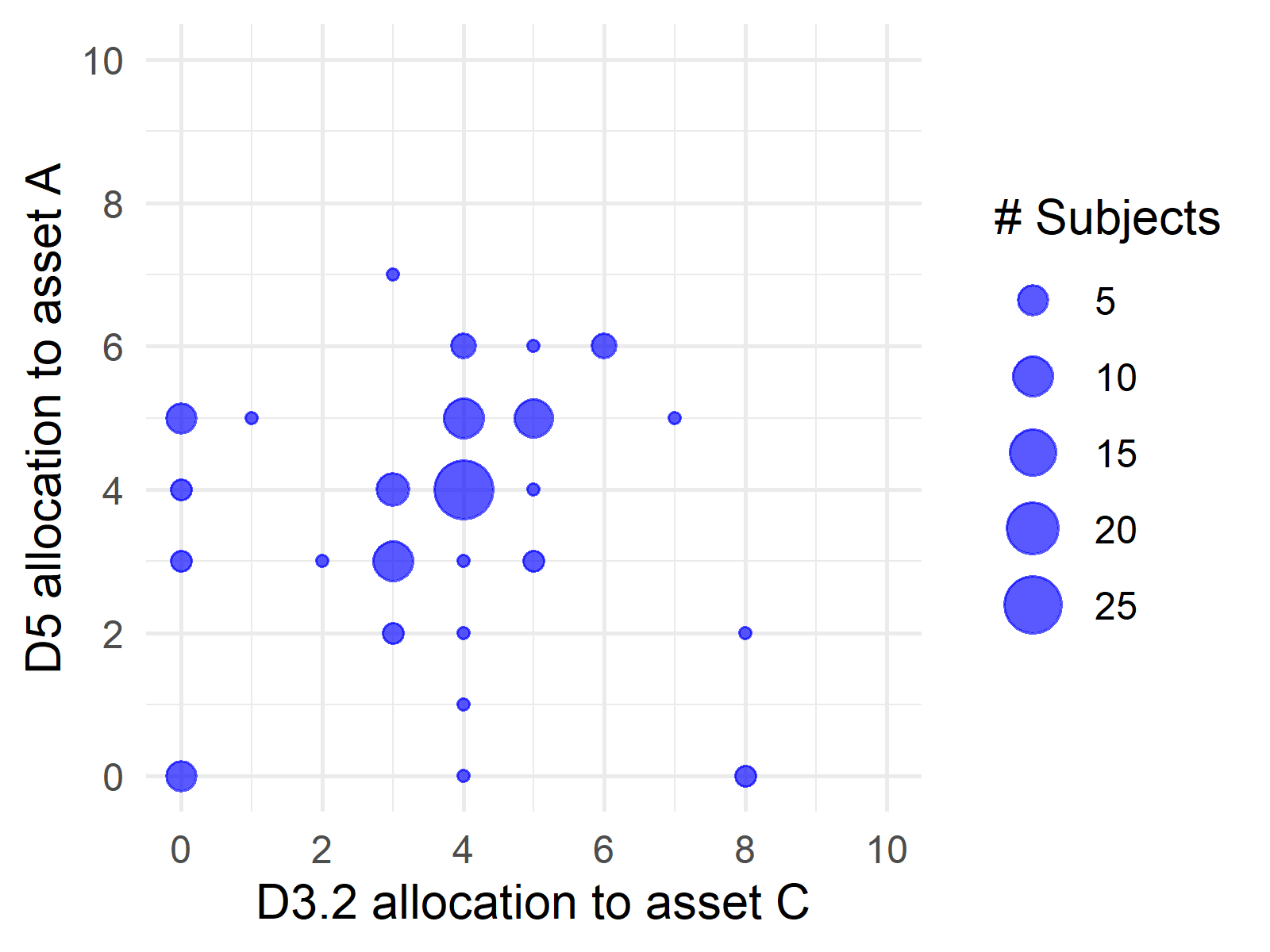
(b) D3.2 and D5 Allocations

To compare how our subjects perform to this benchmark, Figure 1a plots the joint distribution of their allocations in D1. The x-coordinate describes their allocation to Asset A in D1.1, and the y-coordinate their allocation to Asset C in D1.2. The above discussion shows that broad bracketers will have allocations on the y-axis, and a risk-averse broad bracketer will select the allocation $\left(x_{A}^{1,1},x_{C}^{1,2}\right)=(0,14)$. Any narrow bracketer will select an allocation with $x_{A}^{1,1}\leq 5$, and any risk-averse narrow bracketer will select $x_{C}^{1,2}=8$. The plot shows that few subjects are close to consistent with broad bracketing, and only a single subject makes an allocation close to the prediction of risk-averse broad bracketing. Narrow bracketing with risk aversion is consistent with the modal allocation of $\left(x_{A}^{1,1},x_{C}^{1,2}\right)=\left(4,8\right)$.

In our design, narrow bracketing makes strong predictions across decisions that have a part in common. For instance, D3.2 and D5 both ask subjects to allocate 10 tokens between identical assets with identical prices. A narrow bracketer would make the same allocation in each of the two parts. To illustrate, Figure 1b plots each subject’s allocation in D3.2 against their allocation in D5. The x-coordinate describes their allocation to Asset C in D3.2, and the y-coordinate their allocation to its counterpart, Asset A in D5. A narrow bracketer’s choices will fall on the 45-degree line as required by NB-WARP, and the farther the allocations are from that line the farther the subject is from narrow bracketing. In the plot, we can see that this prediction of narrow bracketing holds exactly for 54 of the 99 subjects. We visually represent all the data underlying our tests in Online Appendix.

4.2. Risk and Social Experiments: Revealed Preference Tests

We begin by performing the direct revealed preference tests of bracketing developed in Section 1: NB-WARP, BB-WARP, and BB-Mon (Table 3).

		Risk				Social
# errors		0	1	2		0	1	2
NB-WARP (D1.1 and D5)		56	76	89		45	70	77
NB-WARP (D1.2 and D4))		56	74	81		63	78	82
NB-WARP (D3.2 and D5)		54	76	83		49	75	80
NB-WARP (D1.1 and D3.2)		49	76	85		51	83	87
NB-WARP (all)		29	44	61		28	54	64
BB-WARP (D1 and D2)		13	20	87		16	20	94
BB-Mon (D1)		12	13	15		14	14	14
BB-Mon (D3)		14	16	18		17	17	18
BB-Mon (both)		7	8	10		12	12	12
# subjects		99				102
Entries count the # of subjects who pass test at the listed error allowance.

Table 3. Tests of NB-WARP and BB-WARP

Very few subjects are broad bracketers. There is only a single pair of decisions (D1 and D2) where choices could directly violate BB-WARP. For that pair, we test BB-WARP by comparing the final bundle for D1 to the final bundle for D2: for any choice of $x^{2,1}$ in D2 with $x_{A}^{2,1}\leq 8$, the same final bundle can be achieved in D1. In each of Risk and Social, only 20% of subjects are within one error of passing BB-WARP. Even fewer subjects are consistent with BB-Mon than with BB-WARP. In Risk and Social respectively, we find that 8% and 12% of subjects are within one error of passing BB-Mon in both decisions. Looking separately at D1 and D3, between 13% - 17% of subjects are within one error of passing BB-Mon.

All told, the BB-WARP and BB-Mon tests provide evidence showing that 80%-92% of subjects are not broad bracketers. These rates of violations of broad bracketing are qualitatively similar to, but higher than, those found by Tversky & Kahneman, (1981) (73%) and Rabin & Weizsäcker, (2009) (28%-66%), and very close to the structural estimates of the latter (89%). In these prior experiments, each part consisted of a pairwise choice, so failures to broadly bracket are detected only for a particular range of risk preferences. In contrast, there are many ways a subject could reveal their failure to bracket broadly in our experiments, which gives us more power to detect failures.

While previous work can only falsify broad bracketing, our design allows us to test narrow bracketing as well. We test NB-WARP by comparing the allocations in each of the two parts that appear in multiple decisions. Specifically, NB-WARP requires that a subject makes the same choice in D1.1, D3.2, and D5, and the same choice in D1.2 and D4. Far more subjects pass each NB-WARP test than either BB-WARP or BB-Mon. Between 75-77% of subjects in Risk and 69-81% of subjects in Social are within one error of passing each of the pairwise NB-WARP tests. Allowing for one error, 44% and 53% of subjects pass all possible NB-WARP tests in Risk and Social, respectively.

Result 1.

When allowing for one error, 45% and 53% of subjects pass NB-WARP, 20% and 20% pass BB-WARP, and 8% and 12% pass BB-Mon in the Risk and Social Experiments, respectively.

We next conduct revealed preference tests of symmetric versions of the three models considered using the entire set of decisions for each subject. Symmetry is a natural restriction in our experiments: the two states (dice rolls of 1-3 and 4-6) are equally likely in Risk, and the two other individuals (Person A and Person B) are anonymous in Social. The restrictions implied by symmetry reduce the need to compare across decisions and make our tests more demanding. For example, all three tests make point predictions in D2 and D4. Random behavior has a 0.001% chance or less of passing either BB- or NB-SARP with one error, and a 0.3% chance of passing the PNB Algorithm with one error. Table 4 shows how many subjects pass each test.

		Risk				Social
# errors		0	1	2		0	1	2
NB-SARP		23	34	43		15	36	44
BB-SARP		0	0	0		8	10	10
PNB		49	59	71		31	58	69
PNB-PE		51	63	75		39	67	76
# subjects		99				102
Entries count the # of subjects who pass each test at the listed error allowance.

Table 4. Full Tests of Symmetric Models

We compare results of the tests allowing for up to one error. We find that no subjects pass BB-SARP in Risk, and only 10% of subjects pass it in Social. However, 34-35% of subjects in each experiment pass NB-SARP. While fewer subjects pass BB-SARP than either BB-WARP or BB-Mon, a similar number of subjects pass all NB-WARP restrictions with one error and the more demanding NB-SARP with two errors. These results show that a plurality of our subjects are well-described as narrow bracketers.

Our test of partial-narrow bracketing diagnoses how many of those who fail BB-SARP and NB-SARP behave consistently with intermediate degrees of bracketing. We find that 15% of subjects in Risk and 12% of subjects in Social pass the PNB test but neither BB-SARP nor NB-SARP when allowing for one error. Only 4% of subjects in Risk and 9% of subjects in Social pass the PNB-PE test but not the PNB test.

Result 2.

When allowing for one error relative to each test, 34% and 35% of subjects pass NB-SARP, 0% and 10% of subjects pass BB-SARP, while an additional 25% and 12% of subjects pass the PNB test but neither NB- nor BB-SARP, in the Risk and Social Experiments, respectively.

The tests reported in Result 2 require both that preferences are symmetric and that choices reveal strict preferences. Consequently, subjects with linear preferences, such as those who maximize expected or total payoffs, may fail our tests. A subject with linear preferences makes the same choices in any dataset regardless of how they bracket, so the presence of linear preferences does not bias our results in favor of a given type of bracketing. Five subjects in Risk and two subjects in Social make choices consistent with linearity throughout the experiment. Of these seven subjects, one each in Risk and in Social pass the tests for narrow bracketing. The other subject in Social is within one error of passing all tests of broad bracketing. Two other subjects in Risk always allocated their entire portfolio to Assets B/D, consistent with either risk-seeking or risk-neutral expected utility preferences. Consequently, these two pass BB-WARP, BB-Mon, and NB-WARP but not NB-SARP or BB-SARP with symmetry. The remaining three subjects are not within two errors of passing any of the tests. We thus conclude that the lower pass rates of BB-SARP and NB-SARP tests with the symmetry assumption is almost entirely due to the additional power of these tests, rather than by systematic failures of subjects to have symmetric preferences.

4.3. Shopping Experiment: Induced-Value Tests

The tests of our predictions thus far assume that utility is not observed. When utility is known, as in our Shopping Experiment, narrow and broad bracketing each make unique predictions in each decision. To test the models, we compare how far each subject’s choices are from each model’s predictions (Table 5).

		D1				D3				Both				Full
# errors		0	1	2		0	1	2		0	1	2		0	1	2
NB		23	23	60		53	65	69		20	21	49		15	16	40
BB		20	21	27		23	24	24		12	14	17		11	13	15
PNB		44	45	95		76	91	98		32	36	68		26	29	56
PNB-PE		44	45	95		76	93	98		32	36	70		26	29	57
# subjects		101
Entries count the # of subjects who pass each test at the listed error allowance.

Table 5. Shopping Tests

Testing the point predictions of narrow bracketing in each of Decisions 1 and 3, 23% and 64% of subjects are respectively within one error of the predictions of narrow-bracketing, while 21% are consistent in both. Allowing for two errors raises pass rates to 59% for Decision 1 and 49% for both. Looking at the full set of implications of narrow-bracketing on all choices made in the experiment, 40% of subjects are within two errors of passing.

In contrast, 21%, 24%, and 14% of subjects are within one error of being consistent with broadly-bracketed maximization in Decisions 1, 3, and both, respectively. When allowing for two errors, those numbers remain similar. Using all decisions in the experiment, only 15% of subjects are within two errors of being consistent with all implications of broad-bracketed maximization. PNB describes less than 2% of the remaining subjects.

Since we induce the payoff function, we are able to compute the value of $\alpha$ that best fits a subjects behavior (up to the limits imposed by discretization of the budget sets) under the assumption that the induced value function acts as their utility function. To that end, we compute the point predictions of the partial-narrow bracketing model for each $\alpha\in\{0,0.01,0.02,\dots,0.99,1\}$ for Decisions 1 and 3, and obtain distinct predictions for nine intervals of $\alpha$. We assign each subject to the range of $\alpha$ for which their choices exhibit the fewest errors relative to that range’s predictions. We find that 64% of subjects are classified to a range that includes full narrow bracketing, $\alpha=1$, and 24% are classified to a range that includes full broad bracketing, $\alpha=0$. Of the remaining subjects, none are best described by $\alpha\in[0.25,0.71]$. This suggests that even those subjects who are not exactly described by either broad or narrow bracketing are close.

4.4. Classifying subjects to models

The tests thus far do not make any adjustment for the fact that partial-narrow bracketing nests narrow and broad bracketing as polar cases, and can thus accommodate more behavior. To compare the predictive success of each model at the subject level, we use a subject-level implementation of the Selten score (Selten,, 1991; Beatty & Crawford,, 2011). For each subject and each model (symmetric versions for Risk and Social, using the induced value function for Shopping), we calculate the number of errors the subject exhibits relative to that model. Then, we calculate the number of possible choice combinations in the experiment that are consistent with that model and that number of errors – the model-error pair’s “predictive area”. We divide the predictive area by the total number of possible combinations of choices in the experiment to compute the measure for each subject $i$ and model $m\in\text{\{broad, narrow, PNB},\text{ PNB-PE}\}$ as $\text{predictive\_success}_{i,m}=1-\frac{\#\text{predictive\_area\_for\_}i,m}{\#\text{all\_possible\_choices}}$. We use all choices made in the experiment to assign each subject to the model with the highest predictive success; in cases where every rationalizing model-error pair for a subject would rationalize more than one million possible combinations of choices in our experiment, we categorize them as “Unclassified”.

	Percent Selten Score Maximized
	Risk	Social	Shopping
Broad Bracketing	2.02	9.80	26.73
	(0.35,7.81)	(4.32,15.29)	(17.99,35.48)
Narrow Bracketing	77.78	75.49	67.32
	(69.49,86.06)	(67.10,83.87)	(57.98,76.67)
PNB	7.07	1.96	3.96
	(3.13,14.51)	(0,4.68)	(0.13,7.78)
PNB-PE	0	3.92	0.99
	(0,0)	(0.22,7.61)	(0,2.84)
Unclassified	13.13	8.82	0.99
	(6.42,19.83)	(3.46,14.18)	(0,2.91)
To calculate confidence intervals, we assume that the model of bracketing is multinomially
distributed with fixed strike rate within each treatment and calculate the Wilson, (1927b) score.

Table 6. Classification of subjects

Across the three experiments, we classify 67-78% of subjects as narrow bracketers (Table 6). In contrast, 2%, 10%, and 27% of subjects are classified as broad bracketers in the Risk, Social, and Shopping Experiments respectively. However, 7%, 6%, and 5% were classified to one of the two partial-narrow bracketing models. After adjusting for predictive power, partial-narrow bracketing does not help explain very many subjects’ behavior.

To form confidence intervals, we assume that model of bracketing is multinomially distributed with fixed strike rate within each treatment. We calculate confidence intervals according to the Wilson, (1927a) score. In all three treatments, the lower bound of the interval for narrow bracketers exceeds the upper bound of the intervals for all other models of bracketing. Most other intervals overlap, but there are significantly more broad bracketers than partial-narrow bracketers in the Shopping Experiment.

Result 3.

Judging each model’s fit by its predictive success, 67-78% of subjects are classified as narrow bracketers, 2-27% are classified as broad bracketers, and 5-7% are classified as partial-narrow bracketers across the three experiments.

4.5. Aggregate analysis

Our preceding analysis focuses on subject-level tests, which reveal substantial heterogeneity in how people bracket. The data do not support treating individuals as a “representative” subject. As in other contexts, we reject the null hypothesis that average subject behavior satisfies BB-WARP: a matched-pairs t-test comparing aggregate bundles in D1 to D2 in Risk and Social ($p<0.001$ for Risk, $p<0.001$ for Social) strongly rejects the null hypothesis. The aggregate data are more, but not perfectly, consistent with narrow bracketing, in line with our findings from individual-level analysis. In our Risk and Social Experiments, matched-pairs t-tests of NB-WARP that separately compare average bundles in D1.1 to D5, D3.2 to D5, and D1.2 to D4 fail to reject the null hypothesis ($p=0.84,0.16,0.97$ respectively for Risk, $p=0.38,0.13,0.19$ for Social). However in our Shopping Experiment, we reject both narrow and broad bracketing at the aggregate level when we separately compare allocations in D1.1, D1.2, D3.1, and D3.2 to the point predictions of each of narrow and broad bracketing (eight t-tests total, $p=0.06$ for D1.1 test of narrow bracketing, $p<0.001$ for all other tests). These tests reinforce that our main individual-level analysis detects meaningful heterogeneity across subjects, whereas aggregate tests can produce misleading conclusions. For example, with only aggregate-level tests, one might incorrectly find in favor of partial-narrow bracketing, even though we only classify five subjects in the Shopping Experiment to that model.

5. Robustness and Secondary Analyses

To study how choice architecture mediates bracketing, we conducted an online version of our Risk Experiment that varied the presentation in a two-by-two design. First, the “Examine” treatment instructed the subject to “First, examine both accounts, then purchase your investments” in the instructions, tested this in a quiz question, then included that text at the top of each two-part decision screen; the “Basic” treatment did not. Second, the “Tabs” treatment presented each part of a decision as a separate HTML tab (analogous to our separate pages in our paper experiments), whereas the “Side-by-Side” treatment presented parts of a decision side-by-side on the same screen (analogous to Tversky & Kahneman, 1981). We recruited 200 US-based subjects from Prolific Academic to participate and randomly assigned each to one of the four treatment pairs.

We also replicated our Shopping experiment online with 46 subjects from Prolific Academic. We implemented the Side-by-Side and Examine interventions, eliminated the quantity-restricted sale in D2, and provided subjects with a calculator instead of a payoff table. We provide detailed screenshots and results in the Online Supplement.

Below, we discuss what we learn from our online experiments’ treatment effects in section 5.1 and non-choice data in section 5.7. We explore the robustness of our tests of broad bracketing to extremeness aversion, investigate the possibility of order effects or learning, and perform statistical tests of the differences we find across the domains.

5.1. Effects of choice architecture

We find almost no effect on choices from either of the two interventions in the Online Risk Experiment. The online subject pool is more slanted towards narrow bracketing than our original Pen-and-paper study. Pass rates for each NB-WARP test are higher, and pass rates for BB-WARP and BB-Mon are generally lower. Only 2 of 200 subjects pass BB-SARP when allowing for two errors, and these two, and only these two, are classified as broad bracketers according to Selten score. In contrast, 96 subjects pass NB-SARP when allowing 1 error, and 84.5% are classified as narrow bracketers by Selten score. Both subjects are in the Examine and Tabs treatment, though neither treatment has a statistically significant effect on the rate of broad bracketing ($p=0.22,p=0.24$, for Fisher’s exact tests of the Examine and Tabs treatments, respectively). Within the Tabs group, Examine does not have a statistically significant effect ($p=0.20$, Fisher’s exact test). We similarly find no effect of the treatments on the rates of narrow bracketing ($p=1.00$ for both, Fisher’s exact tests).

In addition, the Online Shopping Experiment implemented both Examine and Side-by-Side. We classified 5 out of 46 (10.86%) subjects to broad bracketing and 33 (71.74%) to narrow. The rate of narrow bracketing did not change much, while the rate of broad bracketing slightly decreased relative to the pen-and-paper Shopping Experiment ($p=0.03$, Fisher’s exact test).

All-in-all, this suggests that the low rates of broad bracketing we find are not overly sensitive to varying the choice architecture to encourage broad bracketing. We caution against over-interpreting this result since broad bracketing was so rare in all treatments. The shift to an online interface and the Prolific subject pool may have had more effect than any of the nudges. We suspect that more extreme nudges and decision aids might be more effective.

5.2. Effects of Extremeness Aversion

As we describe in Section 1, broad bracketing requires a corner solution in at least one part of any multi-part decision. Evidence from other contexts suggests that some subjects may be extremeness averse and avoid corner choices. For example, subjects in linear public good games tend not to play the Nash strategy of making no contributions. However, in non-linear public good games where the Nash strategy requires a positive but not complete contribution, subjects play the equilibrium strategy more frequently (see e.g. Section 2 of Vesterlund,, 2016, for a discussion). Extremeness aversion could affect our conclusions about broad bracketing and its prevalence relative to narrow bracketing.

Non-extreme allocations in two-part decisions lead to violations of BB-Mon. However, few additional subjects are consistent with a relaxation of BB-Mon that allows for subjects to be close to, but not necessarily at, a corner when required. Formally, we say that a subject passes Extremeness-Averse (EA-)BB-Mon if they are within 2 tokens of making an extreme allocations in each decision required by BB-Mon. Without allowing for any errors, 3 subjects in Risk and 0 subjects in Social pass EA-BB-Mon but not BB-Mon. Allowing for 2 errors, 14 subjects in Risk and 3 subjects in Social pass EA-BB-Mon but not BB-Mon. Far more subjects (43 in Risk and 44 in Social) pass NB-SARP at that error-level than pass EA-BB-Mon. Moreover, fewer pass EA-BB-Mon when allowing for two errors than one would expect if people chose uniformly randomly.

This suggests that the effect of extremeness aversion on our tests is probably not too large. The evidence still suggests heterogeneity in bracketing, with a plurality best described as narrow bracketers, even after adjusting for extremeness aversion. Two additional pieces of evidence lend additional support to this assertion. First, a similar number of subjects are consistent with broad bracketing in decisions that require two corner choices as are consistent in decisions that require only one corner choice. Second, the ratio of broad to narrow bracketers does not vary much across treatments in a follow-up experiment for which only one of the two treatments requires a corner choice. Unfortunately, the data is too noisy to draw strong conclusions. We elaborate on this evidence in the Online Supplement.

5.3. Welfare losses and measurement

So far, we have focused on identifying how our subjects bracketed. We apply our classification to quantify in dollar terms the payoffs forgone by narrow bracketers. We also illustrate how looking at aggregate data can lead to misleading inferences (Table 7). A narrow bracketer’s preference parameters should be measured using parts as the unit of observation, and broad bracketer’s should use decisions as the unit of observation. Using the wrong unit of observation, necessary for an aggregate analysis with heterogeneous bracketing, leads to misleading conclusions about preferences. We focus on the Social and Shopping Experiments because there are only two participants classified as broad bracketers in Risk.

Panel A
		Payoff loss ($)
		D1.1	D1.2	D1	D3.1	D3.2	D3	D5	$n$
Risk		0.39	0	0.39	0	0.35	0.35	0.38	99
	NB	0.40	0	0.40	0	0.38	0.38	0.41	77
	BB	0	0	0	0	0.20	0.20	0.30	2
Social		0.47	0	0.47	0	0.46	0.46	0.49	102
	NB	0.51	0	0.51	0	0.51	0.51	0.49	77
	BB	0	0	0	0	0.03	0.03	0.44	10
Shopping		0.55	0.52	1.05	1.00	0.85	1.24	0.05	101
	NB	0.22	0.07	1.41	0.01	0.07	1.67	0.03	68
	BB	1.20	1.31	0.29	3.65	2.92	0.11	0.04	27
“Payoff loss” columns report total $ loss (Shopping), loss in expected value (Risk), and
average loss per recipient (Social) compared to expected/average value maximization. We
evaluate each part on its own in columns D1.1 and D3.2 and integrate across parts in
columns D1 and D3. In D1.2 and D3.1 all allocations have no loss in Risk and Social.

Panel B
		Payoff difference ($)
		D1.1	D1.2	D1	D3.1	D3.2	D3	D5	$n$
Risk		4.24	2.24	5.39	1.88	4.70	4.51	3.79	99
	NB	3.47	0.91	3.91	0.70	3.72	3.98	3.24	77
	BB	12.00	9.00	3.00	3.00	7.60	4.60	6.60	2
Social		3.10	2.39	1.54	2.29	3.35	1.91	2.58	102
	NB	1.64	0.51	1.62	0.60	1.68	1.68	2.17	77
	BB	12.00	12.00	0.00	10.00	11.34	1.46	2.56	10
“Payoff difference” columns report the difference in $ allocations across the two states or people.

Table 7. Losses and payoff differences by parts and decisions

In Shopping, we directly measure dollar losses of a person’s choices relative to the induced value function. When looking narrowly at D1.1 (ignoring D1.2), it would look like subjects’ choices on average forgo $0.55 in payment. However, this number is only $0.22 for subjects classified to narrow bracketing versus $1.20 for subjects classified to broad bracketing. The latter number illustrates how a broad bracketer’s choices can appear irrational if we ignore the full relevant decision context that they account for. When looking at the decision level, the average subject forgoes $1.05 in payments. However, broad bracketers only forgo $0.29 on average, while narrow bracketers forgo an average of $1.41. Looking at a one-part decision, D5, shows that narrow and broad bracketers make roughly similar optimization errors, on average, in one-part rounds. These calculations show that narrow bracketers forgo substantial payoffs as a result of how they bracket. Subjects also give up substantial expected or aggregate payoffs in Risk and Social, but risk or inequality aversion make interpreting this as a welfare loss more ambiguous.

The “Payoff difference” columns of Table 7 illustrate how it is easy to obtain misleading inferences about how subjects make the equity-efficiency trade-off. In the one-part decision D5, narrow bracketers implemented allocations that differed by an average of $2.17 between A and B, while the corresponding average difference is $2.56 for broad bracketers ($p=0.18$, rank sum test comparing D5 allocations). Narrow and broad bracketers make similar trade-offs between equity and efficiency from one-part decisions. Yet if we look at D1.2 or D3.1 on its own, ignoring the other part of the decision, we would incorrectly infer that broad bracketers care mainly about efficiency, while narrow bracketers make near-equal allocations on average, consistent with inequity aversion. We would obtain an opposite conclusion by looking at D1 as a whole, where narrow bracketers’ decision-level allocations involve some inequality on average, but all broad bracketers make perfectly equal final allocations.

5.4. Differences across experiments

The fraction of subjects classified to broad bracketing varies across experiments, from 1% for Online Risk to 27% in Pen-and-paper Shopping. There is a significant difference in broad bracketing rates between Pen-and-paper Shopping and each of Risk and Social ($p<0.01$, Fisher’s exact test) as well as between the Online and Pen-and-paper Shopping experiments ($p<0.01)$. However, narrow bracketing rates varied much less, from 67% to 78% across Pen-and-paper experiments, with no significant differences in these rates ($p>0.10$ for all pairwise Fisher’s exact tests). Nor was there a significant difference in narrow bracketing rates between the Online and Pen-and-paper versions of Risk and Shopping ($p>0.10$ for both Fisher’s exact tests). Explanations for the higher rate of broad bracketing in Shopping and lower rate in Risk include the more naturalistic setting, the presence of an objectively-correct payoff function, and cognitive difficulties specific to choice under risk (as suggested by Martínez-Marquina et al., 2019). We cannot distinguish between these explanations.

5.5. Non-choice data and bracketing

We can use our online experiments to examine how the choice process differs across subject-level bracketing classification. The paucity of broad bracketers in both experiments hinders our ability to find relationships between the two. However, the data do seem to reject the extreme view that narrow bracketers always completely ignore other parts of the decision. For example, approximately a quarter seem to give some consideration to both parts of the decision.

In the Tabs versions of the Online Risk Experiment, we record whether each subject clicked on both tabs before making their final choices. Only 28 of 102 subjects that did so in both D1 and D3 had enough information to bracket broadly. While this includes the 2 broad bracketers, a large majority of the subjects with sufficient information to bracket broadly fail to do so. Of the 28, 22 were in the Examine-Tabs treatment, and 6 were in the Basic-Tabs treatment ($p<0.01$, Fisher’s exact). The prompt was effective at increasing this click pattern, but it did not significantly affect the classification to broad bracketing ($p=0.20$, Fisher’s exact). Clearly, paying attention to both parts of a decision is necessary to bracket broadly. However, the fraction of narrow bracketers among those who paid attention was not substantially different than the fraction among those who did not (21 of 28 versus 61 of 74, $p=0.41$, Fisher’s exact). At the other extreme, we find that 33 subjects made their final choice in each of D1 and D3 before having seen both parts, and thus could not have been broad bracketing; 29 of these subjects are classified as narrow bracketers.

The Online Shopping Experiment provided subjects with a calculator instead of a payoff table. The average (median) number of calculations was 10.40 (12) for broad bracketers, 12.21 (8) for narrow bracketers, and 12.86 (10) for all subjects. As a whole, intensity of calculator use does not differ much between broad and narrow bracketers.

In contrast, patterns of calculator use differ across types of bracketers. Ex-ante, we expected that plugging in bundles that are feasible in the decision as a whole (e.g. (9, 11) for D3) to the calculator (a “broad calculation”) would predict broad bracketing, and that plugging in a bundle that is available in a part of a decision but lies below the decision-level feasible set (e.g. (5,5) for D3) to the calculator (a “narrow calculation”) would predict narrow bracketing. We classify nine of ten subjects of who made a narrow calculation as narrow bracketers. However, we only classify three of 16 subjects who made at least one such “broad calculation” as broad bracketers. Indeed, nine of the 16 are classified as narrow bracketers. In addition, we classify seven of the eight subjects who never use the calculator as narrow bracketers.

In summary, the non-choice data suggest diversity in the relationship between consideration and narrow bracketing. Click patterns across tabs in the Tabs treatment of the Online Risk Experiment and calculator use in the Shopping Experiment suggest that about a quarter of narrow bracketers appear to follow a choice process that involves only considering one part at a time. This is consistent with an extreme form of narrow bracketing in both process and choice. But this same data also shows that a quarter or more of narrow bracketers gave some consideration to both parts before making at least one of their 2-part decisions. The seemingly weak link between broader consideration and broadly-bracketed choices suggests why the interventions we designed to encourage broad bracketing in the Online Risk Experiment were not very effective.

6. Conclusion

Across our experiments, at least twice as many subjects were classified as narrow bracketers than as broad bracketers. A majority of people tend to narrowly bracket, while a noticeable minority broadly bracket. While many of our subjects are not well-described by either broad or narrow bracketing, our novel tests of partial-narrow bracketing suggest that it does not do much better after adjusting for predictive power. This suggests that applications should calibrate a population mix of broad and narrow bracketers rather than a representative agent model with a calibrated partial-narrow bracketing parameter (as in Barberis & Huang,, 2007).

Bracketing rates differ across tasks, domains, and subject pools. While our framework is well-suited to detect and to measure these differences, it is less well-suited to determine why these differences persist. Non-choice data, as we collected in the online follow up experiment, can help. It seems to rule out uniform explanations for why so many bracket narrowly, such as lack of awareness of complementarities across parts. We think understanding why people bracket the way they do is an interesting direction for future work.

Appendix A Theoretical Appendix: Proofs, Derivations, and PNB Algorithm

Proof of Theorem 1.

One can follow the usual proof that SARP holds if and only if a dataset is rationalizable by a complete and transitive preference relation to establish the result with a preference relation; see e.g. Mas-Colell et al.,, 1995. Establishing rationalization with a utility function requires a bit more work. We provide an argument below as we are unaware of one in the literature.

Given $\mathcal{O}=\left(x^{i},B^{i}\right)_{i=1}^{N}$ for either $\mathcal{O}=\mathcal{D}^{NB}$ or $\mathcal{O}=\mathcal{D}^{BB}$, set $X^{\prime}=\cup_{i}B^{i}$. Observe that each $B^{i}$ is a compact set, either by assumption (for $\mathcal{O}=\mathcal{D}^{NB}$) or since the finite sum of compact sets is compact (for $\mathcal{O}=\mathcal{D}^{BB}$). Thus $X^{\prime}$ is also compact. It is therefore bounded as a subset of $\mathbb{R}^{n}$. Let $X$ be a closed ball centered at $0$ containing $X^{\prime}$.

Let $\succsim$ be the transitive closure of $P^{\mathcal{O}}$ defined on $X$. We show that $\succsim$ is closed as a subset of $X\times X$. First, note $P^{\mathcal{O}}$ itself is closed as a finite union of the closed sets $\{(y,z)\in X\times X:y\geq z\}$ and $\{x^{i}\}\times B^{i}$ for all $i=1,\dots,N$. Second, we show that $y\succsim z$ if and only if there exist $y_{1},y_{2},\dots,y_{K-1},y_{K}$ so that $y_{i}P^{\mathcal{O}}y_{i+1}$ for all $i$, $y_{1}=y$, and $y_{K}=z$ where $K\leq 2N+1$. Consider any $y\succsim z$. By definition, there exist $y_{1},y_{2},\dots,y_{K}$ so that $y_{i}P^{\mathcal{O}}y_{i+1}$ for all $i$, $y_{1}=y$, and $y_{K}=z$ and there is no shorter sequence that establishes $y\succsim z$. If $y_{j}\geq y_{j+1}$ and $y_{j+1}\geq y_{j+2}$ for some $i$, then $y_{j}\geq y_{j+2}$, and we can construct a shorter sequence by leaving $y_{j+1}$ out. If $y_{j}\not\geq y_{j+1}$, then $y_{j}=x^{i(j)}$ and $y_{j+1}\in B^{i(j)}$ for some $i(j)$. Then, $y_{k}\neq y_{j}$ for all $k>j$ by SARP, so at most one index $j^{\prime}$ has $i(j^{\prime})=i$ for each $i$. Therefore, the longest possible shortest sequence alternates $\geq$ with direct revelations from choice. There can be no more than $2N+1$ of these, so $K\leq 2N+1$. Moreover, since we can trivially append $y_{K+1}=y_{K}$ to the end of such sequences, we can consider only sequences with exactly $2N+1$ in what follows.

Now, pick any sequence $(y_{m},z_{m})_{m=1}^{\infty}$ contained in $\succsim$ that converges to $(y,z)$. Then, there exists $y_{m}^{2},\dots,y_{m}^{2N}$ so that $y_{m}P^{\mathcal{O}}y_{m}^{2}P^{\mathcal{O}}\dots P^{\mathcal{O}}y_{m}^{2N}P^{\mathcal{O}}z_{m}$. The sequence $(y_{m},y_{m}^{2},\dots,y_{m}^{2N},z_{m})$ has a convergent subsequence $(y_{m_{k}},y_{m_{k}}^{2},\dots,y_{m_{k}}^{2N},z_{m_{k}})$ since $X\times\dots\times X$ is compact by the Tychonoff Theorem. Let $(y^{*},y^{2*},\dots,y^{2N*},z^{*})$ be its limit. Since $P^{\mathcal{O}}$ is closed, $y^{*}P^{\mathcal{O}}y^{2*}P^{\mathcal{O}}\dots P^{\mathcal{O}}y^{2N*}P^{\mathcal{O}}z^{*}$. Finally, $\left(y^{*},z^{*}\right)=\left(y,z\right)$ since $\left(y_{m},z_{m}\right)\rightarrow\left(y,z\right)$. Hence $\succsim$ is closed.

Now, apply Levin,, 1983’s Theorem, as in Nishimura et al.,, 2017, to get a utility function $U$ from $X$ to $[0,1]$ so that $x\succ y$ implies $U(x)>U(y)$ and $x\succsim y$ implies $U(x)\geq U(y)$. Since $\geq$ is included in $\succsim$, $U(\cdot)$ is increasing. Since $x^{i}\succ y$ for all $y\in B^{i}\setminus\left\{x^{i}\right\}$, $U(x^{i})>U(y)$ for all $y\in B^{i}\setminus\left\{x^{i}\right\}$. Extending to all of $\mathbb{R}_{+}^{n}$ is straightforward, simply set $U(y)=V(y)$ whenever $y\notin X$ for an arbitrary increasing function $V(\cdot)$ picked so that $V(y)>1$ for all $y$.

Proof of Theorem2.

Fix $\alpha$ and $\mathcal{D}$. For every decision $t$, define the lottery

$$p^{t}=\frac{\alpha K_{t}}{\alpha K_{t}+(1-\alpha)}\left(\frac{1}{K_{t}},x^{t,k}\right)_{k=1}^{K_{t}}+\frac{(1-\alpha)}{\alpha K_{t}+(1-\alpha)}\left(1,x^{t}\right),$$

and $Y\subseteq\mathbb{R}^{n}$ to be a finite set that includes the union of the supports of $p^{1},\dots,p^{T}$ and the vector $0$. It will be convenient to take $Y$ equal to this set but this is inessential. Denote by $\Delta Y$ the finite support lotteries over $Y$. Consider the set

$$Q_{Y}^{t}=\left\{\frac{\alpha K_{t}}{\alpha K_{t}+(1-\alpha)}\left(\frac{1}{K_{t}},y^{k}\right)_{k=1}^{K_{t}}+\frac{(1-\alpha)}{\alpha K_{t}+(1-\alpha)}\left(1,y\right)\in\Delta Y:\exists z^{k}\in B^{t,k}\text{ so that }y^{k}\leq z^{k}\,\&\ y\leq\sum z^{k}\right\}$$

is a finite set of lotteries over $Y$ that includes $p^{t}$ and any others that are affordable. The ancillary dataset

$$\mathcal{D}_{Y}^{\alpha}=\left\{\left(p^{t},Q_{Y}^{t}\right)\right\}_{t=1}^{T}$$

is strictly rationalizable by expected utility if and only if $\mathcal{D}$ is rationalizable by $\alpha$-partial-narrow bracketing.

If so, then there exists an EU preference $V$ over $\Delta Y$ so that

$$V\left(p^{t}\right)>V\left(q^{t}\right)\,\forall q^{t}\in Q_{Y}^{t}\backslash p^{t}$$

for all $t$. Let $v$ be the utility index of $V$ and extend to $\mathbb{R}_{+}^{n}$ by

$$u^{*}(z)=\max_{y\leq z,y\in Y}v(y).$$

Then for any $t$ and $y^{t,1}\times\dots\times y^{t,K_{t}}\in B^{t,1}\times\dots\times B^{t,K_{t}}\setminus\left\{x^{t,1}\times\dots\times x^{t,K_{t}}\right\}$,

$$\alpha\sum_{k}u^{*}(x^{t,k})+(1-\alpha)u^{*}(x^{t})=\kappa_{t}V\left(p^{t}\right)>\kappa_{t}\max_{q^{t}\in Q_{Y}^{t}\backslash p^{t}}V\left(q^{t}\right)\geq\alpha\sum_{k}u^{*}(y^{t,k})+(1-\alpha)u^{*}\left(\sum_{k=1}^{K_{t}}y^{t,k}\right)$$

where $\kappa_{t}=\alpha K_{t}+(1-\alpha)$. To find a strictly increasing $u$, let $u^{**}$ be a strictly increasing extension of $v$. Choosing $\epsilon>0$ small enough, for $u=(1-\epsilon)u^{*}+\epsilon u^{**}$,

$$\alpha\sum_{k}u(x^{t,k})+(1-\alpha)u(x^{t})>\alpha\sum_{k}u(y^{t,k})+(1-\alpha)u(\sum_{k=1}^{K_{t}}y^{t,k})$$

for all $t$ and any $y^{t,1}\times\dots\times y^{t,K_{t}}\in B^{t,1}\times\dots\times B^{t,K_{t}}\setminus\left\{x^{t,1}\times\dots\times x^{t,K_{t}}\right\}$, establishing that $\mathcal{D}$ is rationalized by $\alpha$-PNB.

Conditions under which $\mathcal{D}_{Y}^{\alpha}$ is rationalized by expected utility are well-known. Here, we follow Clark, (1993). As standard, $p$ is directly revealed preferred to $q$, written $p\succ q$, if $p=p^{t}$ and $q\in Q_{Y}^{t}\setminus\left\{p^{t}\right\}$ for some decision $t$. Define $p\succsim q$ if $p\succ q$ or $p=q$. We say that $p$ is indirectly reveal preferred via independence to $q$, written $p\tilde{\succsim}q$, whenever there exist $r,p_{1},\dots,p_{n},q_{1},\dots,q_{n}\in\Delta Y$, $\alpha\in(0,1]$, and $\lambda_{1},\dots,\lambda_{n}>0$ so that

$$\alpha p+(1-\alpha)r =\sum_{i=1}^{n}\lambda_{i}p_{i}$$

$$\alpha q+(1-\alpha)r =\sum_{i=1}^{n}\lambda_{i}q_{i}$$

$$p_{i} \succsim q_{i}\text{ for all }i=1,\dots,n$$

$$\sum_{i=1}^{n}\lambda_{i} =1$$

and $p\tilde{\succ}q$ holds whenever at $p_{i}\succ q_{i}$ for some $i$. The Linear Axiom of Revealed Preference (LARP) is that $q\tilde{\succsim}p$ implies that $p\tilde{\succ}q$ does not hold. Theorem 3 of Clark, (1993), combined with the finiteness of $\mathcal{D}^{\alpha}$, implies that $\tilde{\succsim}$ has an expected utility rationalization. Conclude $\mathcal{D}^{\alpha}$ satisfies LARP if and only if $\mathcal{D}$ is rationalized by $\alpha$-partial-narrow bracketing.

The following algorithm inputs $\mathcal{D}^{\alpha}$ and outputs $1$ if and only $\mathcal{D}$ is rationalized by $\alpha$-partial-narrow bracketing for any rational number $\alpha\in[0,1]$. For concreteness, label $Y=\left\{y_{1},y_{2},\dots,y_{m}\right\}$. We identify each $p\in\Delta Y$ with the $p\in\mathbb{R}^{m}$ so that $p_{i}=p(y_{i})$.

Define the matrix $A$ with a column equal to $p^{t}-q$ for each $q\in Q_{Y}^{t}\backslash p^{t}$ and every $t$. $A$ is an $D\times m$ matrix interpreted as strict preference, where $D$ is the number of data points extracted. Let $\vec{1}$ be a $D\times 1$ matrix of ones and

$$\hat{A}=\left[\begin{array}[]{c}A\\ \vec{1}\end{array}\right].$$

Let $\hat{b}$ be an $m+1$ vector with the first $m$ components $0$ and the last $1$.

Note that if $p\tilde{\succsim}q$, then there exists $\alpha>0,$$\lambda_{i}\geq 0$, and $p_{i}\succsim q_{i}$ for $i=1,...,m$ so that

$$\alpha(p-q)=\sum_{i=1}^{m}\lambda_{i}(p_{i}-q_{i})$$

and $\sum_{i=1}^{m}\lambda_{i}=1$. Each $p_{i}-q_{i}$ corresponds to a column of $A$, so this is equivalent to $p-q\in C=cone(co(\left\{A_{1},\dots,A_{D}\right\}))$ where $A_{i}$ is the $i$th column of $A$. LARP holds when $p-q\in C$ implies $q-p\notin C$, or, equivalently, if and only if $0\notin C$. That is, there does not exist $\phi^{1},\dots,\phi^{D}\geq 0$ so that $\sum\phi^{i}=1$ so that $\sum_{i=1}^{D}\phi^{i}A_{i}=0$, which is equivalent to $\hat{A}\phi=\hat{b}$.

Solve the system

$$\min_{y\in\mathbb{R}^{m+1}}y^{T}\hat{b}$$

$$s.t. \hat{A}^{T}y\geq 0$$

for $y$. The Ellipsoid algorithm provides a polynomial-time solution to this. Let $y^{*}$ be the solution, if one exists. There are two cases:

Case 1: There is no solution to $\hat{A}^{T}y\geq 0$ or $y^{*}$ satisfies $y^{*T}\hat{b}\geq 0$. Then, Farkas’s Lemma implies there exists $\phi\geq 0$ so that $\hat{A}\phi=\hat{b}$. LARP fails by the above, so return $0$.

Case 2: The program is unbounded below or $y^{*T}\hat{b}<0$. Then, Farkas’s Lemma implies there does not exist any $\phi\geq 0$ so that $\hat{A}\phi=\hat{b}$. LARP is satisfied by the above, so return 1.

To specialize the above to PNB-PE, we perform the analysis part by part rather than decision by decision. Let $p^{t,k}=(\alpha,x^{t};(1-\alpha),x^{t,k})$, $Y\subseteq\mathbb{R}^{n}$ be a finite set that includes the union of the supports of the lotteries $p^{t,k}$, and

$$Q_{Y}^{t,k}=\left\{\left(\alpha,y;(1-\alpha),y^{\prime}\right)\in\Delta Y:\text{$\exists$}x\in B^{t,k}\text{ so that }y^{\prime}\leq x+x^{t,-k}\,\&\,y\leq x\right\}$$

Repeating the above with the ancillary dataset

$$\mathcal{D}_{Y}^{PE,\alpha}=\left\{\left(p^{t,k},Q^{t,k}\right)\right\}_{(t,k)}$$

replacing $\mathcal{D}^{\alpha}$ establishes the result.

$\square$

Theorem 3 (Identification of $\alpha$.).

Suppose that $u$ is a known differentiable and strictly quasi-concave function and $\mathcal{D}$ is rationalized by partial-narrow bracketing. Further suppose that for some $t,k$, $B^{t,k}$is a Walrasian budget set for prices $p^{t,k}$, and $n=2$, $\frac{p_{1}^{t,1}}{p_{2}^{t,1}}\neq\frac{p_{1}^{t,2}}{p_{2}^{t,2}}$, $\underset{x_{1}\rightarrow 0^{+}}{\lim}\frac{\partial u(x_{1},x_{2})}{\partial x_{1}}=+\infty$ for all $x_{2}>0$, and $\underset{x_{2}\rightarrow 0^{+}}{\lim}\frac{\partial u(x_{1},x_{2})}{\partial x_{2}}=+\infty$ for all $x_{1}>0$.
Then, there exists a unique $\alpha$ that rationalizes choices.

Proof of Theorem 3.

Suppose the assumptions of the Theorem are satisfied. In the partial-narrow bracketing model, the marginal utility per dollar of spending on good $j$ in decision $k$ is given by:

$$\frac{1}{p_{j}^{t,k}}\left((1-\alpha)\frac{\partial u(x^{t,1}+x^{t,2})}{\partial x_{j}}+\alpha\frac{\partial u(x^{t,k})}{\partial x_{j}}\right)$$

for $k=1,2$. By the limit conditions, if $\alpha>0$, then $x_{j}^{t,k}>0$ for $j=1,2$ and $k=1,2$; thus $x_{1}^{t,k}=0$ or $x_{2}^{t,k}=0$ implies $\alpha=0$. If $\frac{1}{p_{2}^{t,k}}\partial u(x^{t,k})/\partial x_{2}=\frac{1}{p_{1}^{t,k}}\partial u(x^{t,k})/\partial x_{1}$ for both $k$, then set $\alpha=1$. Now suppose that $\frac{1}{p_{2}^{t,k}}\partial u(x^{t,k})/\partial x_{2}\neq\frac{1}{p_{1}^{t,k}}\partial u(x^{t,k})/\partial x_{1}$ and an interior allocation is chosen in budget set $k$. The first-order condition for an interior maximizer equates the marginal utility per dollar across the two goods; rearranging this condition, we obtain

$$\alpha=\frac{\frac{1}{p_{1}^{t,k}}\partial u(x^{t,1}+x^{t,2})/\partial x_{1}-\frac{1}{p_{2}^{t,k}}\partial u(x^{t,1}+x^{t,2})/\partial x_{2}}{\frac{1}{p_{1}^{t,k}}\partial u(x^{t,1}+x^{t,2})/\partial x_{1}-\frac{1}{p_{2}^{t,k}}\partial u(x^{t,1}+x^{t,2})/\partial x_{2}+\frac{1}{p_{2}^{t,k}}\partial u(x^{t,k})/\partial x_{2}-\frac{1}{p_{1}^{t,k}}\partial u(x^{t,k})/\partial x_{1}}$$

for $k=1,2$. It remains to verify that the expression on the right-hand side always lies in the interval $(0,1)$. Since $\frac{1}{p_{2}^{t,k}}\partial u(x^{t,k})/\partial x_{2}\neq\frac{1}{p_{1}^{t,k}}\partial u(x^{t,k})/\partial x_{1}$, the solution satisfies $(1-\alpha)\left(\frac{1}{p_{1}^{t,k}}\frac{\partial u(x^{t,1}+x^{t,2})}{\partial x_{1}}-\frac{1}{p_{2}^{t,k}}\frac{\partial u(x^{t,1}+x^{t,2})}{\partial x_{2}}\right)=\alpha\left(\frac{1}{p_{2}^{t,k}}\frac{\partial u(x^{t,k})}{\partial x_{2}}-\frac{1}{p_{1}^{t,k}}\frac{\partial u(x^{t,k})}{\partial x_{1}}\right)$. Thus, if $\alpha\in(0,1)$, the denominator and numerator have the same sign, and the denominator is strictly larger in absolute value – therefore the expression is well-defined and thus $\alpha$ is identified from choices.

$\square$

Joint implications of narrow and broad bracketing

To study the joint implications of broad and narrow bracketing we consider endowment bracketing in a rich domain. We thus suppose that we observe an infinite dataset on all decisions that each consist of a binary part and a second degenerate part summarized by its only available bundle $z$. Suppose that when a person has bundle $z\in\mathbb{R}_{+}^{n}$ in their second part and must make a binary choice, they apply a complete, transitive, continuous, and strictly increasing binary relation $\succsim_{z}$ (call such a binary relation a well-behaved preference). In this domain, we say that a person broadly brackets if $x\succsim_{z}y\iff x+z\succsim_{\text{$\underline{0}$}}y+z$; a person narrowly brackets if $x\succsim_{z}y\iff x\succsim_{z^{\prime}}y$ for all $z^{\prime}\in\mathbb{R}_{+}^{n}$.

Theorem 4.

The family of well-behaved preferences $\{\succsim_{z}\}_{z\in\mathbb{R}_{+}^{n}}$ satisfies both narrow and broad bracketing if and only if there exists a vector $u\in\mathbb{R}_{++}^{n}$ such that $x\succsim_{z}y$ if and only if $x\cdot u\geq y\cdot u$.

Proof.

The “if” direction is immediate. So now consider the “only if” direction.We do so by constructing an additive utility representation for $\succsim_{\text{$\underline{0}$}}$. Since $\succsim_{\text{$\underline{0}$}}$ is a well-behaved preference relation, for each $x\in\mathbb{R}_{+}^{n}$ there exists a unique number $\kappa\in\mathbb{R}_{+}$ such that $x\sim_{\text{$\underline{0}$}}\kappa e$ where $e=(1,1,\dots,1)$; define $u(x)=\kappa$ for each $x$ and the corresponding $\kappa$. By strict monotonicity, $u$ represents $\succsim_{\text{$\underline{0}$}}$, and by continuity, $u$ is continuous. Pick any $x,y\in\mathbb{R}_{+}^{n}$. By NB, $x\sim_{y}u(x)e$ and $y\sim_{u(x)e}u(y)e$, so by BB and transitivity $x+y\sim_{0}y+u(x)e\sim_{0}u(x)e+u(y)e$, so $u(x+y)=u(x)+u(y)$. Since $x,y$ were arbitrary, $u(x)=u\cdot x$ for some $u\in\mathbb{R}_{++}^{n}$ by Theorem 1 in Chapter 5 of Aczél, (1966). ∎

Derivations of predictions and their experimental implementations.

First, observe that if relation $P$ is acyclic, it must be anti-symmetric.

Derivation of Prediction 1 (NB-WARP)

Suppose $x^{t^{\prime},k^{\prime}}\in B^{t,k}\subseteq B^{t^{\prime},k^{\prime}}$. By the definition of $P$ in NB-SARP, $x^{t^{\prime},k^{\prime}}Px$ for all $x\in B^{t^{\prime},k^{\prime}}\backslash\{x^{t^{\prime},k^{\prime}}\}$. Since $B^{t,k}\subseteq B^{t^{\prime},k^{\prime}}$, it follows that $x^{t^{\prime},k^{\prime}}Px$ for all $x\in B^{t,k}\backslash\{x^{t^{\prime},k^{\prime}}\}$. But if $x^{t,k}\neq x^{t^{\prime},k^{\prime}}$, the definition of $P$ would imply $x^{t,k}Px^{t^{\prime},k^{\prime}}$, which would violate acyclicity. Thus $x^{t,k}=x^{t^{\prime},k^{\prime}}$.

Discretized implementation in our experiment.

In all of our tests of NB-WARP, we have $B^{t,k}=B^{t^{\prime},k^{\prime}}$ exactly. We thus test NB-WARP exactly, without needing to adjust for discreteness.

Derivation of Prediction 2 (BB-WARP)

Suppose $x^{t^{\prime}}\in B^{t}\subseteq B^{t^{\prime}}$. By the definition of $P$ in BB-SARP, $x^{t^{\prime},k^{\prime}}Px$ for all $x\in B^{t^{\prime}}\backslash\{x^{t^{\prime}}\}$. Since $B^{t}\subseteq B^{t^{\prime}}$, it follows that $x^{t^{\prime}}Px$ for all $x\in B^{t}\backslash\{x^{t^{\prime}}\}$. But if $x^{t}\neq x^{t^{\prime}}$, the definition of $P$ would imply $x^{t}Px^{t^{\prime}}$, which would violate acyclicity. Thus $x^{t}=x^{t^{\prime}}$.

Discretized implementation in our experiment.

In the Risk and Social experiments, $\text{co}B^{1,1}+\text{co}B^{1,2}\subseteq\text{co}B^{2,1}$. In particular, $B^{2,1}=\left\{\left(\$0,\$28\right);\left(\$2,\$26\right);\dots;\left(\$28,\$0\right)\}\right\}$, whereas $B^{1,1}+B^{1,2}=\left\{\left(\$0,\$28\right);\left(\$1,\$27\right);\dots;\left(\$16,\$12\right);\left(\$17,\$10.80\right);\dots;\left(\$26,\$0\right)\right\}$. Consider two cases.

If $x_{A}^{2,1}\leq\$16$, the bundle chosen in $B^{2,1}$ is exactly affordable in $B^{1,1}+B^{1,2}$. The caveat is that the set $B^{1,1}+B^{1,2}$ has a higher resolution in this range. We do not adjust for this, implicitly interpreting their choice from $B^{2,1}$ as revealing their preferences over the $\text{co}B^{2,1}$. However, if this leads a subject to fail BB-WARP, if their preferences are well-behaved, they would choose in $B^{2,1}$ one of the closest bundles to their preferred bundle in $\text{co}B^{2,1}$ and be within one error away from passing BB-WARP.

However, if $x_{A}^{2,1}>\$16$, then the person reveals a sufficiently strong preference for person/state A over B that their desired bundle in $B^{2}$ is not affordable in $\text{co}B^{1,1}+\text{co}B^{1,2}$ and thus they trivially pass BB-WARP.

Derivation of Prediction 3 (BB-Mon)

Suppose $x_{1}^{t,2}>0$, $x_{2}^{t,1}>0$, and $p_{1}^{t,1}\leq p_{2}^{t,1}$, $p_{1}^{t,2}>p_{2}^{t,2}$. Let $\epsilon=\min\{x_{1}^{t,2},x_{2}^{t,1}\}$. Consider the alternative pair of choices $\left(y^{t,1},y^{t,2}\right)$ given by $y^{t,1}=\left(x_{1}^{t,1}+\frac{p_{2}^{t,1}}{p_{1}^{t,1}}\epsilon,x_{2}^{t,1}-\epsilon\right)$ and $y^{t,2}=\left(x_{1}^{t,2}-\epsilon,x_{2}^{t,2}+\frac{p_{1}^{t,2}}{p_{2}^{t,2}}\epsilon\right)$. By construction, $\left(y^{t,1},y^{t,2}\right)$ is affordable. We have that

$y_{1}^{t,1}+y_{1}^{t,2}=x_{1}^{t,1}+x_{1}^{t,2}+\frac{p_{2}^{t,1}-p_{1}^{t,1}}{p_{1}^{t,1}}\epsilon\geq x_{1}^{t,1}+x_{1}^{t,2}$, and

$y_{2}^{t,1}+y_{2}^{t,2}=x_{2}^{t,1}+x_{2}^{t,2}+\frac{p_{1}^{t,2}-p_{2}^{t,2}}{p_{2}^{t,1}}\epsilon>x_{2}^{t,1}+x_{2}^{t,2}$

where the inequalities respectively follow from $p_{1}^{t,1}\leq p_{2}^{t,1}$ and $p_{1}^{t,2}>p_{2}^{t,2}$. But $x^{t}Py^{t}$ would violate monotonicity; thus such an $x^{t,1},x^{t,2}$ pair could not pass BB-SARP.

Discretized implementation in our experiment.

The argument in the proof applies with minimal modification to our discretized experiment, and thus we apply the conditions directly.

References

- Abeler & Marklein, (2017) Abeler, Johannes, & Marklein, Felix. 2017. Fungibility, labels, and consumption. Journal of the European Economic Association, 15(1), 99–127.
- Aczél, (1966) Aczél, J. 1966. Lectures on Functional Equations and Their Applications. New York and London: Academic Press.
- Andreoni & Miller, (2002) Andreoni, James, & Miller, John. 2002. Giving according to GARP: An experimental test of the consistency of preferences for altruism. Econometrica, 70(2), 737–753.
- Baillon et al., (2022) Baillon, Aurélien, Halevy, Yoram, & Li, Chen. 2022. Randomize at your own Risk: on the Observability of Ambiguity Aversion. Econometrica, 90(3), 1085–1107.
- Barberis & Huang, (2007) Barberis, N., & Huang, M. 2007. The loss aversion/narrow framing approach to the equity premium puzzle. Pages 199–229 of: Mehra, R (ed), Handbook of Investments: Equity Premium. Amsterdam: North-Holland.
- Barberis, (2012) Barberis, Nicholas. 2012. A model of casino gambling. Management Science, 58(1), 35–51.
- Barberis & Huang, (2009) Barberis, Nicholas, & Huang, Ming. 2009. Preferences with frames: a new utility specification that allows for the framing of risks. Journal of Economic Dynamics and Control, 33(8), 1555–1576.
- Barberis et al., (2006) Barberis, Nicholas, Huang, Ming, & Thaler, Richard H. 2006. Individual preferences, monetary gambles, and stock market participation: A case for narrow framing. American Economic Review, 96(4), 1069–1090.
- Baron & Kemp, (2004) Baron, Jonathan, & Kemp, Simon. 2004. Support for trade restrictions, attitudes, and understanding of comparative advantage. Journal of Economic Psychology, 25(5), 565–580.
- Beatty & Crawford, (2011) Beatty, Timothy KM, & Crawford, Ian A. 2011. How demanding is the revealed preference approach to demand? American Economic Review, 101(6), 2782–95.
- Blow & Crawford, (2018) Blow, Laura, & Crawford, Ian. 2018. Observable Consequences of Mental Accounting. Working Paper.
- Bolton & Ockenfels, (2000) Bolton, Gary E, & Ockenfels, Axel. 2000. ERC: A theory of equity, reciprocity, and competition. American Economic Review, 90(1), 166–193.
- Camerer, (2004) Camerer, Colin F. 2004. Prospect Theory in the Wild: Evidence from the Field. Pages 148–162 of: Camerer, Colin F, Loewenstein, George, & Rabin, Matthew (eds), Advances in Behavioral Economics. Princeton University Press.
- Charness & Rabin, (2002) Charness, Gary, & Rabin, Matthew. 2002. Understanding social preferences with simple tests. Quarterly Journal of Economics, 117(3), 817–869.
- Choi et al., (2007) Choi, Syngjoo, Fisman, Raymond, Gale, Douglas, & Kariv, Shachar. 2007. Consistency and heterogeneity of individual behavior under uncertainty. American Economic Review, 97(5), 1921–1938.
- Clark, (1993) Clark, Stephen A. 1993. Revealed preference and linear utility. Theory and Decision, 34(1), 21–45.
- Cox et al., (2015) Cox, James C, Sadiraj, Vjollca, & Schmidt, Ulrich. 2015. Paradoxes and mechanisms for choice under risk. Experimental Economics, 18(2), 215–250.
- Crawford & De Rock, (2014) Crawford, Ian, & De Rock, Bram. 2014. Empirical revealed preference. Annual Review of Economics, 6(1), 503–524.
- Dhami, (2016) Dhami, Sanjit. 2016. The foundations of behavioral economic analysis. Oxford University Press.
- Ebert & Strack, (2015) Ebert, Sebastian, & Strack, Philipp. 2015. Until the bitter end: on prospect theory in a dynamic context. American Economic Review, 105(4), 1618–33.
- Ellis & Piccione, (2017) Ellis, Andrew, & Piccione, Michele. 2017. Correlation Misperception in Choice. American Economic Review, 107(4), 1264–92.
- Evers & Imas, (2019) Evers, Ellen, & Imas, Alex. 2019. Mental accounting, similarity, and preferences over the timing of outcomes. Tech. rept.
- Exley & Kessler, (2018) Exley, Christine L, & Kessler, Judd B. 2018. Equity concerns are narrowly framed. Tech. rept. National Bureau of Economic Research.
- Eyster & Weizsäcker, (2016) Eyster, Erik, & Weizsäcker, Georg. 2016. Correlation neglect in portfolio choice: Lab evidence. SSRN Working Paper 2914526.
- Fisman et al., (2007) Fisman, Raymond, Kariv, Shachar, & Markovits, Daniel. 2007. Individual preferences for giving. American Economic Review, 97(5), 1858–1876.
- Galperti, (2019) Galperti, Simone. 2019. A theory of personal budgeting. Theoretical Economics, 14(1), 173–210.
- Gneezy & Potters, (1997) Gneezy, Uri, & Potters, Jan. 1997. An experiment on risk taking and evaluation periods. Quarterly Journal of Economics, 112(2), 631–645.
- Hastings & Shapiro, (2018) Hastings, Justine, & Shapiro, Jesse M. 2018. How are SNAP benefits spent? Evidence from a retail panel. American Economic Review, 108(12), 3493–3540.
- Hastings & Shapiro, (2013) Hastings, Justine S, & Shapiro, Jesse M. 2013. Fungibility and consumer choice: Evidence from commodity price shocks. Quarterly Journal of Economics, 128(4), 1449–1498.
- Heimer et al., (2020) Heimer, Rawley, Iliewa, Zwetelina, Imas, Alex, & Weber, Martin. 2020. Dynamic Inconsistency in Risky Choice: Evidence from the Lab and Field. Tech. rept. SSRN Working Paper 3600583.
- Hines & Thaler, (1995) Hines, James R, & Thaler, Richard H. 1995. The flypaper effect. Journal of Economic Perspectives, 9(4), 217–226.
- Imas, (2016) Imas, Alex. 2016. The realization effect: Risk-taking after realized versus paper losses. American Economic Review, 106(8), 2086–2109.
- Kahneman & Tversky, (1979) Kahneman, Daniel, & Tversky, Amos. 1979. Prospect Theory: An Analysis of Decision under Risk. Econometrica, 47(2), 263–291.
- Koch & Nafziger, (2019) Koch, Alexander K, & Nafziger, Julia. 2019. Correlates of narrow bracketing. Scandinavian Journal of Economics, 121(4), 1441–1472.
- Kőszegi & Matějka, (2020) Kőszegi, Botond, & Matějka, Filip. 2020. Choice simplification: A theory of mental budgeting and naive diversification. Quarterly Journal of Economics, 135(2), 1153–1207.
- Kőszegi & Rabin, (2006) Kőszegi, Botond, & Rabin, Matthew. 2006. A model of reference-dependent preferences. Quarterly Journal of Economics, 121(4), 1133–1165.
- Levin, (1983) Levin, Vladimir L. 1983. Measurable Utility Theorems for Closed and Lexicographic Preference Relations. Soviet Mathematics Doklady, 27(3), 639–43.
- Lian, (2019) Lian, Chen. 2019. A theory of narrow thinking. Tech. rept. MIT mimeo. Working Paper.
- Martínez-Marquina et al., (2019) Martínez-Marquina, Alejandro, Niederle, Muriel, & Vespa, Emanuel. 2019. Failures in contingent reasoning: The role of uncertainty. American Economic Review, 109(10), 3437–3474.
- Mas-Colell et al., (1995) Mas-Colell, Andreu, Whinston, Michael D., & Green, Jerry R. 1995. Microeconomic Theory. New York: Oxford University Press.
- Mu et al., (2020) Mu, Xiaosheng, Pomatto, Luciano, Strack, Philipp, & Tamuz, Omer. 2020. Background risk and small-stakes risk aversion. arXiv preprint arXiv:2010.08033.
- Nishimura et al., (2017) Nishimura, Hiroki, Ok, Efe A., & Quah, John K.-H. 2017. A Comprehensive Approach to Revealed Preference Theory. American Economic Review, 107(4), 1239–63.
- Odean, (1998) Odean, Terrance. 1998. Are investors reluctant to realize their losses? Journal of Finance, 53(5), 1775–1798.
- O’Donoghue & Sprenger, (2018) O’Donoghue, Ted, & Sprenger, Charles. 2018. Reference-dependent preferences. Pages 1–77 of: Handbook of Behavioral Economics: Applications and Foundations 1, vol. 1. Elsevier.
- Polisson et al., (2020) Polisson, Matthew, Quah, John K.-H., & Renou, Ludovic. 2020. Revealed Preferences over Risk and Uncertainty. American Economic Review, 110(6), 1782–1820.
- Rabin, (2000) Rabin, Matthew. 2000. Risk Aversion and Expected-Utility Theory: A Calibration Theorem. Econometrica, 68(5), 1281–92.
- Rabin & Weizsäcker, (2009) Rabin, Matthew, & Weizsäcker, Georg. 2009. Narrow bracketing and dominated choices. American Economic Review, 99(4), 1508–43.
- Read et al., (1999) Read, Daniel, Loewenstein, George, & Rabin, Matthew. 1999. Choice Bracketing. Journal of Risk & Uncertainty, 19(1-3), 171–197.
- Safra & Segal, (2008) Safra, Zvi, & Segal, Uzi. 2008. Calibration results for non-expected utility theories. Econometrica, 76(5), 1143–1166.
- Samuelson, (1963) Samuelson, Paul. 1963. Risk and uncertainty: A fallacy of large numbers. Scientia, 57(98).
- Selten, (1991) Selten, Reinhard. 1991. Properties of a measure of predictive success. Mathematical Social Sciences, 21(2), 153–167.
- Shefrin & Statman, (1985) Shefrin, Hersh, & Statman, Meir. 1985. The disposition to sell winners too early and ride losers too long: Theory and evidence. Journal of Finance, 40(3), 777–790.
- Smith, (1776 (1904 edition)) Smith, Adam. 1776 (1904 edition). An Inquiry into the Nature and Causes of the Wealth of Nations. London: Methuen & Co.
- Sobel, (2005) Sobel, Joel. 2005. Interdependent preferences and reciprocity. Journal of Economic Literature, 43(2), 392–436.
- Thaler, (1985) Thaler, Richard H. 1985. Mental accounting and consumer choice. Marketing Science, 4(3), 199–214.
- Thaler, (1999) Thaler, Richard H. 1999. Mental accounting matters. Journal of Behavioral Decision Making, 12(3), 183–206.
- Thaler & Johnson, (1990) Thaler, Richard H, & Johnson, Eric J. 1990. Gambling with the house money and trying to break even: The effects of prior outcomes on risky choice. Management Science, 36(6), 643–660.
- Thaler et al., (1997) Thaler, Richard H, Tversky, Amos, Kahneman, Daniel, & Schwartz, Alan. 1997. The effect of myopia and loss aversion on risk taking: An experimental test. Quarterly Journal of Economics, 112(2), 647–661.
- Tversky & Kahneman, (1981) Tversky, Amos, & Kahneman, Daniel. 1981. The framing of decisions and the psychology of choice. Science, 211(4481), 453–458.
- Vesterlund, (2016) Vesterlund, Lise. 2016. Using experimental methods to understand why and how we give to charity. Chap. 2, pages 91–151 of: Kagel, John H., & Roth, Alvin E. (eds), Handbook of Experimental Economics, vol. 2. Princeton, NJ, USA: Princeton University Press.
- Vorjohann, (2020) Vorjohann, Pauline. 2020. Reference-dependent choice bracketing. Tech. rept. University of Exeter. Working Paper.
- Wilson, (1927a) Wilson, E. B. 1927a. Probable inference, the law of succession, and statistical inference. Journal of the American Statistical Association, 22(158), 209–212.
- Wilson, (1927b) Wilson, Edwin B. 1927b. Probable inference, the law of succession, and statistical inference. Journal of the American Statistical Association, 22(158), 209–212.
- Yaari & Bar-Hillel, (1984) Yaari, Menahem E, & Bar-Hillel, Maya. 1984. On dividing justly. Social Choice and Welfare, 1(1), 1–24.
- Zhang, (2023) Zhang, Mu. 2023. Procedural Expected Utility. Tech. rept. Working Paper.