Cataloging the radio-sky with unsupervised machine learning: a new approach for the SKA era

Abstract

We develop a new analysis approach towards identifying related radio components and their corresponding infrared host galaxy based on unsupervised machine learning methods. By exploiting Parallelized rotation and flipping INvariant Kohonen maps (PINK), a self-organising map algorithm, we are able to associate radio and infrared sources without the a priori requirement of training labels. We present an example of this method using $894,415$ images from the Faint Images of the Radio-Sky at Twenty centimeters (FIRST) and Wide-field Infrared Survey Explorer (WISE) surveys centred towards positions described by the FIRST catalogue. We produce a set of catalogues that complement FIRST and describe $802,646$ objects, including their radio components and their corresponding AllWISE infrared host galaxy. Using these data products we (i) demonstrate the ability to identify objects with rare and unique radio morphologies (e.g. ‘X’-shaped galaxies, hybrid FR-I/FR-II morphologies), (ii) can identify the potentially resolved radio components that are associated with a single infrared host and (iii) introduce a “curliness” statistic to search for bent and disturbed radio morphologies, and (iv) extract a set of 17 giant radio galaxies between $700-1100$ kpc. As we require no training labels, our method can be applied to any radio-continuum survey, provided a sufficiently representative self-organising map (SOM) can be trained.

1 Introduction

Radio astronomy will enter its ‘golden age’ as the Square Kilometre Array (SKA) and its pathfinder instruments begin to operate at full capacity over the next decade. This new suite of radio interferometers, including the Low Frequency Array (LOFAR) (van Haarlem et al., 2013), Murchison Widefield Array (MWA) (Tingay et al., 2013; Wayth et al., 2018), Australian Square Kilometre Array Pathfinder (ASKAP) (Johnston et al., 2008), MeerKAT (Jonas & MeerKAT Team, 2016) and the Karl G. Jansky Very Large Array (JVLA) (Perley et al., 2011), offer exceptional gains in sensitivity and survey speeds when compared to previous generations of instruments (Norris, 2017a). They will be capable of routinely producing deep continuum surveys containing tens of thousands of radio sources on timescales as short as hours, a feat that would have taken months of dedicated telescope time some years ago. With this gain in sensitivity and survey speed comes the need to redesign how data analysis and interpretation is performed. Existing efforts that are primarily powered by human ‘intelligence’ are expensive in both time and effort and will not be able to scale to these exceptionally high data volumes.

Among these non-trivial tasks is the process of applying a morphological classification to each of the detected radio sources within some image. This involves describing all of the potentially resolved structure of a single intrinsic object, including situations where some of its components may be separated by some distance (i.e. many units of the resolution element of the instrument).

Tools have been developed to help distribute this classification problem. Perhaps the most successful to date is the Galaxy Zoo online portal (Lintott et al., 2008), a publicly accessible website that allows ‘citizen scientists’ (members of the general public who may not formally be trained in the field) to participate in a broad set of astronomical classification problems alongside domain experts. Especially relevant to this work is Radio Galaxy Zoo (RGZ) (Banfield et al., 2015), a project being operated on the Galaxy Zoo platform. They ask the public to identify related radio components and their infrared host galaxy of complex sources using primarily images from the 1.4 GHz Very Large Array (VLA) FIRST (Becker et al., 1995) and the all-sky WISE (Wright et al., 2010) surveys. RGZ has been successful in producing a dataset that can be used as training sets, allowing for Machine Learning (ML) approaches to contribute to this source classification problem (Lukic et al., 2018; Alger et al., 2018; Wu et al., 2019).

These studies each apply a supervised ML method, where an algorithm needs examples of data with known or trusted attributes (e.g. galaxy/morphology type, redshifts) in order to optimise a cost function and produce a usable model. Without training labels (produced by RGZ or a similar project) these methods can not be used. As radio interferometers each have their own performance characteristics (e.g. observing frequency, angular scale sensitivities), the types of objects and physical processes that each survey can be sensitive to may be vastly different. Some recent work has begun to evaluate how well some supervised ML models can be transferred to datasets they were not trained against (Tang et al., 2019), but it remains to be seen how successful these approaches will be and how far this extrapolation of models and labels can be stretched.

An alternate approach is an unsupervised ML framework. This is a broad set of algorithms that are executed without a priori knowledge about the dataset. Instead the focus is on recognising the structure within a dataset (Ghahramani, 2004). Examples include $k$-means clustering (Lloyd, 1982), Gaussian mixture models (Day, 1969), principal component analysis (Pearson, 1901) and SOM (Kohonen, 1982), the latter being of focus in this study. As there is no error function conditioned against existing labels, the structure that an unsupervised method infers may not correspond to existing classification schemes described by a set of labels. Depending on the ML method chosen, the relationships may be transparently examined, or may be hidden within several layers of complexity, often making it difficult to know exactly what the method has discovered. However, if the structure of the data is understood, then such models can be applied to a variety of problems that may not have been foreseen when they were initially trained.

SOMs have been used in the astronomical literature for a variety of tasks, including the classification of light curves (Brett et al., 2004), clustering and analysis of gigahertz-peaked spectrum sources (Torniainen et al., 2008), detecting structure within point data (Way et al., 2011) and object classification and photometric redshift estimation (Geach, 2012). They operate by constructing a set of prototypes fixed on some regular lattice like structure that are representative of the types of structures seen within a training dataset. Proximity of prototypes upon this lattice represent the level of similarity of the structures those prototypes are describing.

Applying the SOM method onto image datasets may require introducing a redefinition on how similarity is measured. Often we want image processing methods to be invariant to affine transformations (i.e. scaling, flipping, rotation, and translation). For example, the orientation of an active galactic nuclei (AGN) and its radio lobes is not a significant characteristic.

Ralph et al. (2019) approach the problem by using a convolutional auto-encoder to first construct a latent vector (a compressed space that encodes defining characteristics within an image) to minimise the effect of affine transformations, and then train a SOM based on these latent vectors. Although this offers orders of magnitude improvement with regards to training time, the representative features within the neurons are features within the compressed latent vector space and are not directly interpretable without an additional decoding step.

An alternate solution is to attack the affine transform problem directly. PINK is an algorithm that incorporates flipping and rotational invariance into the SOM algorithm (Polsterer et al., 2016). By exploiting products determined during the training process, the SOM itself can be used as a tool to transfer knowledge (Galvin et al., 2019). Given that the SOM requires no training labels and is able to construct prototypes representative of source morphologies, it may prove to be an ideal tool for distinguishing between alternative explanations. For example, it may be able to distinguish the two lobes of a radio AGN from a pair of star forming galaxies.

Galvin et al. (2019) used PINK to create prototypes capable of breaking this degeneracy by including infrared image information, thereby producing prototypes with estimated host galaxy positions.

In our study we investigate how PINK can be used to identify related radio components and their corresponding host galaxy. We present a proof-of-concept method that demonstrates how we can accomplish this without the requirement of training labels. This manuscript is structured as follows. In §2 we describe the construction of a SOM, and in §3 briefly describe our component grouping procedure. The datasets and their preprocessing steps used outlined in §4, and our approach to source collation and catalogue creation is described in §5. We present our results in §6, and discuss improvements and future outlooks in §7. We adopted the cosmology of Hinshaw et al. (2013) where $\Omega_{m}=0.287$, $\Omega_{\lambda}=0.713$ and $H_{0}=$69.3\text{\,}\mathrm{km}\text{\,}{\mathrm{s}}^{-1}\text{\,}{\mathrm{Mpc}}^{-1}$$.

2 Self Organising Maps

SOMs are a type of neural network that constructs a set of features that are representative of those in a training dataset (Kohonen, 1982). They can be thought of as a way of projecting high dimensional data onto a lower dimensional lattice or manifold. Data can be compared to these constructed feature sets using a similarity measure, where the terms ‘closer’ and ‘distant’ refer to data items being similar or dissimilar to items on the SOM lattice, respectively. For a properly trained SOM, each of the major features within the training dataset should be represented by at least one constructed feature without over-representing any single class.

The SOM consists of a set of neurons $n\in N$, each with a position $p$ on the SOM lattice, and a set of prototype weights, $w$. These prototype weights can be initialised in various ways, including random noise following some distribution. For a single training iteration, $i$, an item $t\in T$ is selected, where $T$ is a training dataset, and a similarity measure $\Delta\left(t,w_{p}\right)$ is computed (see §2.1). The neuron most similar to $t$ is the Best Matching Unit (BMU). Once the position of the BMU, $j$, is identified, all prototype weights are updated

$$w^{\prime}_{p}=w_{p}+\left(\phi\left(t\right)-w_{p}\right)\cdot d\left(p,j\right)\cdot l\left(i\right),$$ (1)

where $\phi$ may be necessary to spatially align $t$ onto $w_{p}$. $d$ is the distance component, or neighbourhood function, and $l$ is the time component, or learning rate. $d$ down-weights the updates by an amount that increases with the separation between the position coordinates $p$ and $j$. The exact functional form of this radial decay is arbitrary, but is often parameterised to take the form of a Gaussian,

$$d\left(p,j\right)=\frac{1}{\sigma_{u}\sqrt{2\pi}}\exp\left[{-\frac{1}{2}\left(\frac{s\left(p,j\right)}{\sigma_{u}}\right)}\right],$$ (2)

where $s\left(p,j\right)$ is the separation between $p$ and $j$ lattice coordinate positions and $\sigma_{u}$ is a term used to control the distance updates are propagated (which may also evolve with $i$). The time component $l$ of Equation 1 is a term that further dampens the significance of the weighting updates applied for each $i$. An exponential decay for $l$ could be adopted,

$$l\left(i\right)=\exp\left[-i/\tau\right]$$ (3)

where $\tau$ is a constant to further dampen the evolution of $l$. In the PINK implementation both $\sigma_{u}$ and $l$ are user defined values that do not automatically evolve with increasing $i$.

2.1 Rotation and Flipping Invariance

When dealing with image data, we need methods that are invariant to rotation and flipping transforms. PINK implements a modified Euclidean distance metric that will search for the optimal set of rotation and flipping parameters to align an example image to prototype weights on a SOM. Their measure is formalised as

$$\Delta(t,w_{j})=$$ (4)

$$\underset{\forall\phi\in\Phi}{minimize(\phi)} \sqrt{\sum_{c=0}^{C}\sum_{x=0}^{X}\sum_{y=0}^{Y}\left(w_{j\left(c,x,y\right)}-\phi(t_{c,x,y})\right)^{2}},$$

where $c$ are image channels within $t$ and $w_{j}$, $x$ and $y$ pixel coordinates, and $\phi$ corresponds to an affine image transform taken from a set of transforms $\Phi$. The optimal $\phi$ will describe whether $t$ has to be flipped and the rotation that should be applied to align it with features contained in $w_{j}$. The best matching realisation of $t$ is carried forward to update the entire set of prototypes.

Because the technique is rotationally invariant, we need to avoid the blank corner regions that rotating an image would introduce. The prototypes are therefore a factor of $\sqrt{2}$ times smaller than the input images when a quadrilateral shape is used. PINK performs rotation in a clockwise direction around the central pixel and flips images across the vertical axis.

Computationally generating and comparing all transforms in $\Phi$ is an expensive process. PINK leverages the massive parallel processing capabilities of modern Graphical Processing Units to accelerate the brute force optimisation of Equation 4. With the performance optimisation implemented by PINK, the algorithm scales in linear proportion to the number of images, neurons and transforms. Throughout this study we use PINK v1.1.

3 Overview of Our Approach

Supervised morphological classification algorithms require data to be labelled (e.g. single, double, bent-tail, etc), and the cost of doing so can be prohibitive for all-sky surveys expected from SKA and its pathfinder projects. Furthermore, such labels can often not be transferred to other projects, because of varying resolution, sensitivity, etc. Instead, here we present an unsupervised framework for classifying and identifying objects.

Additionally, by understanding the underlying structure of the training dataset, we can create a framework that is versatile without requiring the training of a new model, unlike typical supervised methods.

For our approach to identifying and cataloguing (potentially resolved) galaxy morphologies across wavebands we train a SOM whose role is to project the high order image data onto a manifold in a lower dimensional space. This space is made up of prototypes with meaningful features constructed by PINK that represent the dominant structures in the training dataset. Since there are only a small number of prototypes compared to the number in the training dataset, we can annotate important features and create descriptive labels for each prototype. The manifold constructed by the SOM is used as the basis to transfer knowledge from the annotated prototypes onto items in the training dataset. We do this by reversing the direction of the mapping carried out against the SOM. Essentially, we use an unsupervised ML algorithm to create a set of classes that are representative of the types of objects in the image data which are then classified by a domain expert. These labels are then transferred back to the original training data. If the training data were representative of a larger set, this transfer of knowledge can be made to previously unseen data.

By using PINK, the solution required to ‘undo’ the affine transformation of an image and map it onto a corresponding neuron is explicitly derived. Therefore, as the world coordinate system (WCS) of each input image is known, features annotated at the pixel level can be converted to absolute sky positions.

Our approach has three main stages,

1. training a representative SOM that exhibits physically meaningful object morphologies,

2. annotating the constructed prototype weights, and

3. transferring these labeled features back onto the training images and collating them into a useable catalogue.

We apply our approach to a combination of radio and infrared images and catalogue data from large surveys. With this combination there is sufficient information to distinguish the host galaxy producing the radio emission and separate unrelated nearby galaxies. The radio catalogue describes individual components, and multiple radio components can share the same host galaxy. Ideally, for any radio component a single infrared source is identified as the host galaxy. Practically though this may not be possible for all radio components, particularly in regions where the infrared image is confused, saturated or simply too faint to be detected in the infrared image.

To maximise the usefulness of this approach, we minimise the initial upfront cost that is required before training can commence. We require a set of catalogued source components and access to their corresponding images. We do not need supplementary information such as redshifts, magnitudes, flux densities.

4 Datasets, Pre-Processing and SOM creation

Distinguishing between morphologies (e.g. AGNs and SFG) requires multi-wavelength information. We therefore use a combination of radio and infrared data. The infrared emission is used to localise the host galaxy, enabling us to distinguish between radio components that are related to a single galaxy versus radio components that happen to be near one another by random chance.

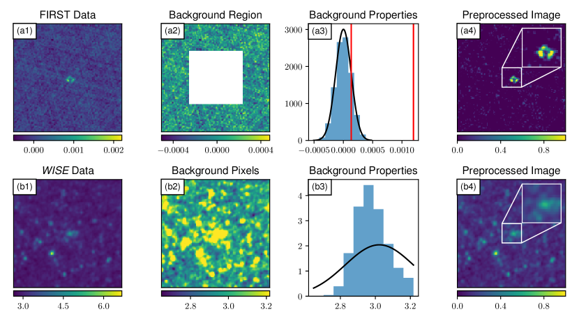
Figure 1: The pre-processing stages applied to the FIRST (top row) and WISE W1 band data (bottom row) for the sky position towards (J2000) RA, DEC = 11:37:34 30:00:10 that contains a known wide angle tailed AGN (Blanton et al., 2004). Panels (a1) and (b1) show the raw FIRST and WISE input images respectively. Panel (a2) shows the masking region used to estimate the background noise statistics of the FIRST radio continuum image of each source. Pixels from this background region make up the histogram in panel (a3). The overlaid Gaussian on this histogram shows the model we construct to replace empty and missing pixel values from the FIRST input images based on the mean and standard deviation of pixels in the background region. The left and right red lines represent the $1\sigma$ lower limit and the $9\sigma$ upper limit used to clip the input FIRST images. The final FIRST pre-processed image, shown in (a4), is produced by applying a MinMax normalisation to the clipped FIRST data. To better emphasize the noise characteristics of the WISE image, we created panel (b2) by applying stretch to hide the brightest pixels of panel (b1). These stretched pixels were used to create the distribution in panel (b3), and their mean and standard deviation were used to establish the overlaid Gaussian profile. The WISE data were then placed onto a logarithmic scale before being normalised onto a zero to one intensity scale, shown as the final pre-processed image in panel (b4). We show the pixel intensity range under each appropriate panel as an accompanying colour bar. The inset figure within (a4) and (b4) show the zoomed region of the centre of each preprocessed image. Pixel values in the original FIRST and WISE images are Jy/beam and Digital Numbers (DN) respectively.

4.1 Radio and Infrared Data

As our base catalogue we used positions of radio components detected from FIRST (Becker et al., 1995; Helfand et al., 2015), a $1.4\text{\,}\mathrm{GHz}$ survey covering over 10,000 deg² of sky conducted with the VLAin the B array configuration. FIRST achieves a resolution of $5\mathrm{″}$ with an rms sensitivity of $0.15\text{\,}\mathrm{mJy}\text{\,}{\mathrm{beam}}^{-1}$. Its positional accuracy is $0.05\mathrm{″}$ for radio components whose flux density is $\sim$$0.75\text{\,}\mathrm{mJy}$. FIRST detected 946,432 radio components with approximately 35% showing resolved structure (Becker et al., 1995). Throughout this study we use the most recent version of the FIRST catalogue. The term radio component refers to a single two-dimensional Gaussian that describes a region of radio emission in an image, parameterised by its on-sky position, brightness, orientation angle and angular size. Extended or highly resolved sources may be described by a collection of radio components.

Complementing this radio survey is the WISE all sky infrared survey (Wright et al., 2010). It is made up of four wavelength bands corresponding to 3.4, 4.6, 12 and 22 $\mu$m (labelled as $W1,W2,W3$ and $W4$) reaching 5$\sigma$ point source sensitivities of 0.08, 0.11, 1. and 6.0 mJy, respectively. The corresponding resolutions for these bands are $6.1\mathrm{″}$, $6.4\mathrm{″}$, $6.5\mathrm{″}$ and $12\mathrm{″}$. This study uses only the W1 band.

4.2 Data Pre-Processing

To build our training dataset, we downloaded $5\mathrm{\prime }$$\times$$5\mathrm{\prime }$ images for each FIRST catalogue position from the appropriate FIRST and WISE image cutout services. Using WCS meta-data that accompanied each image (Greisen & Calabretta, 2002), the WISE $W1$ band data were were placed on the same pixel grid as the FIRST images using bilinear re-interpolation (the same interpolation algorithm used by PINK). In practise this corresponded to a small rotation correction, generally less than $15\mathrm{°}$. PINK is not aware of the WCS and works strictly on pixel intensities when searching for the BMU. Although this reprojection was not strictly required, it was carried out to ensure that the prototype weights could easily be compared across wavelength channels. A small positional error may be introduced from this reprojection, but this would be most drastic for infrared structures towards the border of the images and are minimal.

We then preprocessed the images to enhance feature characteristics. We expand the procedure outlined by Galvin et al. (2019), which we describe below.

FIRST radio continuum images suffer from correlated Gaussian noise and imaging artefacts, both of which are produced by the VLA point spread function (PSF). Although iterative image deconvolution methods (Högbom, 1974, and its modern derivates) have been carried out on these images (Becker et al., 1995), for many bright sources there still remains imaging artefacts that can contaminate the similarity measure and consequently degrade the set of representative features that PINK can construct. To counter both of these issues, a background region was used to estimate the noise properties for each FIRST image. If there were any pixels with a not-a-number (NaN) value (as was the case for images near the edge of a mosaic region) they were replaced by values drawn from a pixel distribution with a mean and standard deviation established by the background region (panel a3 of Figure 1). The $1\sigma$ value of this noise distribution was then subtracted from each pixel to set it as the new zero point. Next, to place more emphasis on the morphological shapes of objects within an image, an upper ceiling of 9$\sigma$ was applied. Finally these images were normalised to a zero to one pixel intensity scale. This procedure is shown in the top row of Figure 1.

WISE images followed a similar set of preprocessing stages. However, neighbouring pixels of WISE images are not correlated in the same way as radio-interferometric images. Because of the weight update process of a SOM, the lack of correlated noise features means that over many iterations the confused infrared images tend to cancel out all but the consistent features. Therefore, no background masking was attempted for these WISE images. We did attempt to characterise the pixel intensity profile only to replace pixels with non-finite NaN values. However, as the noise characteristics of the WISE instrument are not entirely Gaussian and images are approaching the source confusion limit, our approach is only a first order approximation. To avoid any bias potentially introduced by this incomplete profile, sources whose image contained more than twenty pixels to replace were dropped. This often happened when an image was towards the edge of the field of view of the co-added WISE mosaics. If too many pixels are blanked then the potential of clipping out distinguishing structure increases. Finally, WISE images were placed onto a logarithmic scale and a MinMax normalisation was performed following

$$I_{normalized}=\frac{I-\mathrm{min}\left(I\right)}{\mathrm{max}\left(I\right)-\mathrm{min}\left(I\right)},$$ (5)

where $I$ is the image data to be normalised. This process is presented as the bottom row in Figure 1.

The remaining set of successfully preprocessed images were then formed into two-channel images, with 95% and 5% channel weights being applied to the FIRST and WISE $W1$ data respectively. These weights make the Euclidean distance more sensitive to inconsistencies in the radio channel when searching for the BMU. We show the effects of the preprocessing stages in Figure 1.

In Table 1 we show the number of images that failed throughout the data acquisition and preprocessing stages. Note that that there were no images that could not be retrieved from the FIRST server. A total of $894,415$ of the total $946,432$ images centred towards FIRST catalogued radio components were successfully preprocessed and placed into our training dataset.

In principal, we could download images that are centred towards the positions described by an infrared catalogue instead of those from FIRST. This may require some level of curation or subsetting of input images as the source density of the infrared sky is many times higher than the source density of current radio-continuum surveys, and therefore increases the computational requirements of the entire process.

Step	Number
FIRST Components	946,432
WISE Download Failed	268
WISE Reprojection Failed	44
WISE NaN Check Failed	51,705
Training Dataset	894,415

Table 1: An overview of the number of images that were successfully downloaded and preprocessed into our training dataset from the base FIRST radio component catalogue. We include the number of components whose postage stamp image could not be downloaded from the either the FIRST or WISE server, were unable to be reprojected onto a common pixel grid, or did not pass preprocessing steps due to to many missing or invalid WISE pixels (NaN Check Failed).

4.3 Training the SOM

It is difficult to construct a SOM that represents all the features from a complex training dataset, as the small number of neurons tends to be dominated by the most common features in the training dataset. This could be countered by increasing the number of neurons, but this is very computationally expensive. We therefore adopt a training procedure which uses two hierarchical SOM layers, as described below.

4.3.1 Layer One

We trained an initial SOM layer using PINK across five simple stages, which are outlined in Table 2. Within the nomenclature of PINK a single iteration refers to each item in the training dataset being used once to update the prototypes on the SOM. A SOM of $10\times 10$ neurons in a quadrilateral layout was initialised using the PINK options ‘random noise with ‘preferred direction.’ This will initialise weights as uniformly distributed noise between 0-1, and will set pixel intensities across the top-left to bottom-right diagonal to values of one, which attempts to seed the orientation of resolved radio structures in this direction. Throughout all training stages no periodic boundary conditions (i.e. updates that wrap around the edges of the SOM lattice) nor update radius cutoffs (i.e. weight updates only applied to prototypes if they are less than some distance to the BMU) were used. We used a Gaussian neighbourhood function (implemented in PINK) to weigh the updates made to prototype weights. Each training stage has a user defined learning rate that remains constant throughout all iterations. The specifications of each training stage are provided in Table 2.

The goal of the early training stages is to establish the broad layout of features among neurons. This requires only a minimal set of rotations. Subsequent training stages concentrate on the small scale structure. Our first training stage had three iterations and only 48 rotations with increments of $7.5^{\circ}$. Although this introduces the possibility of a small misalignment between an image and prototype ($\sim 6$ pixels in the worst case for our training conditions), the $7.5$ factor of improvement in training time was substantial and justified during these earliest training epochs. The size of the neighbourhood function and learning rate are also the largest, allowing for many prototypes to be modified with each update.

Training	$\sigma_{u}$	$l$	Rotations	Iterations
Stage
1	1.5	0.10	48	3
2	1.0	0.05	92	5
3	0.7	0.05	92	5
4	0.7	0.05	360	5
5	0.3	0.01	360	10

Table 2: Parameters used when training SOMs with PINK throughout this study. The column ‘$\sigma_{u}$’ denotes the one sigma width of the neighbourhood function used to apply prototype updates (Equation 2). The learning rate used for each stage during the weighting update process (Equation 1) is shown in column ‘$l$’.

Training stages two and three begin to slowly reduce the region of influence of each prototype update by shrinking the neighbourhood function and lowering the learning rate. A larger set of rotations are also used to capture some of the more refined details. Finally, stages four and five focus on the smallest level of details by allowing 360 rotations with a small region of influence.

Hyper-parameter selection is important as there are no formal convergence criteria for the SOM algorithm. If the neighbourhood functions is too large, then all prototype weights are modified, whereas a neighbourhood function that is too small will decouple neurons from each other. Similarly if the learning rate is too small the SOM will require a large computation time to train, whereas too large produces abrupt and unstable prototype changes. We converged on these five training stages largely by experimentation across several trials where we qualitatively examined the SOM searching neurons that carried physically meaningful morphologies or other distinguishing characteristics. In practise we found the SOM was most sensitive to the background clipping level applied to the radio images. By virtue of the weight averaging process, we found that PINK was remarkably efficient at extracting the uncleaned remnants of the VLA PSF from below the noise, which consequently became the dominating feature across the SOM.

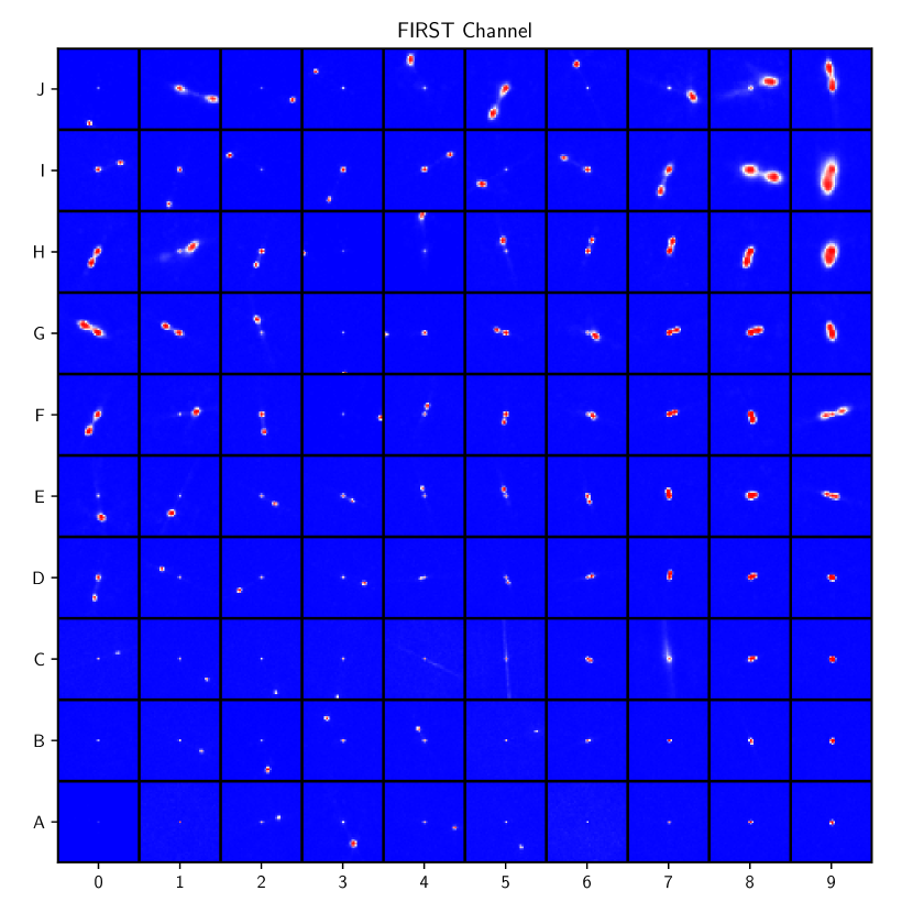
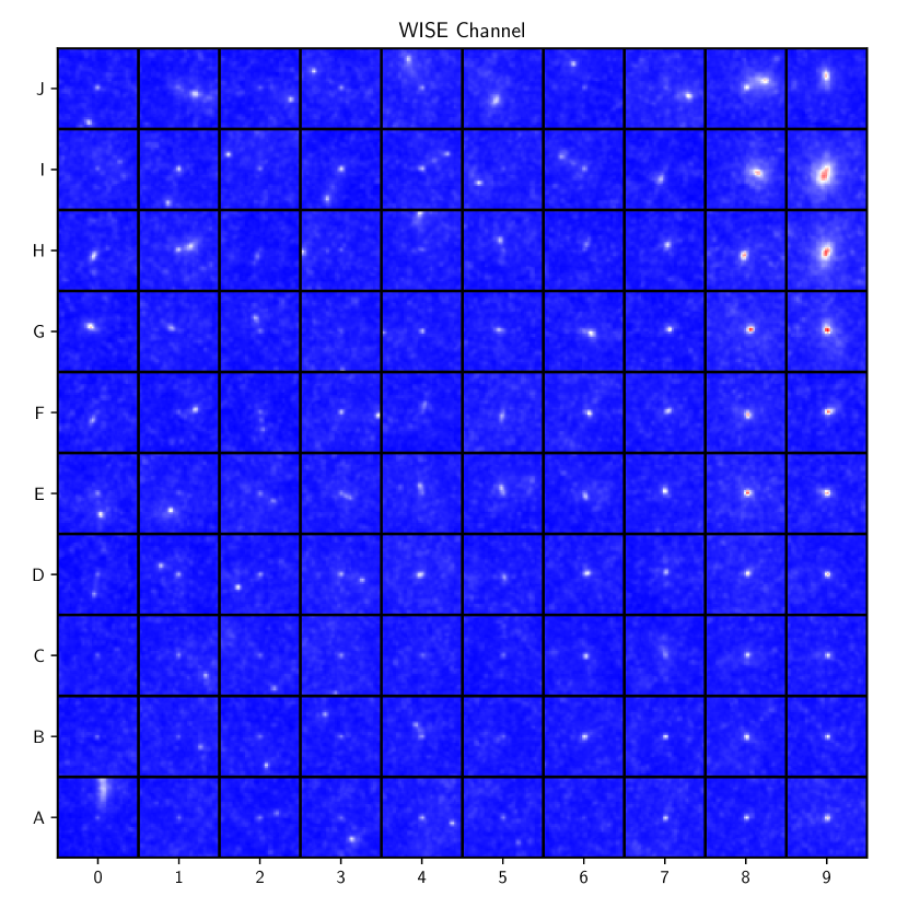
Figure 2: The FIRST (top) and WISE (bottom) channels of the layer one SOM using the preprocessing and training steps described throughout §4.2-4.3.1.

The final Layer One SOM is shown in Figure 2. Across its lattice there is strong evolution of morphologies. Towards the bottom right corner of the FIRST channel near the (B, 8) neuron is a concentration of point source objects without companions. When moving towards (B, 1), these single radio features evolve into two distinct components. The neurons around (E, 4) also possess two separate unresolved radio components without signs of extended morphologies or low level diffuse structure. Towards (H, 1) these features slowly become more pronounced and diffuse. The top right corner near (I, 8) contains the largest set of radio features, with most containing two individual radio components with a clear bridge of diffuse emission connecting them.

The constructed prototypes of the WISE channels show less variety. Most neurons have a single unresolved source. However, some of these unresolved objects are offset from the centre of the neuron (see Figure 3, panel (b2) for an example). For neurons in columns 0 to 4 there is often a secondary infrared component offset from the centre of the neuron. Near (I, 8) there are extended structures in the recovered infrared prototypes.

We emphasise that for the WISE images we applied no background clipping or region masking to images in the training dataset. The structures learnt within the WISE channel have been recovered through what is essentially an image stacking procedure performed by PINK during its prototype weighting update step. The consistent features within individual images re-enforce one another throughout the training stages, and since the instrumental PSF of WISE if far less significant than the synthesised PSF of the VLA, the predominate features in the infrared prototype weights are genuine source morphologies. Without background clipping radio images PINK does a remarkable job of recovering the residual un-cleaned sidelobe artefacts of the synthesised PSF that remain below the noise level and treats these as distinguishing features in the radio prototype weights.

4.3.2 Layer Two

A domain expert may notice that some expected morphological features are missing from Figure 2. Because the SOM makes data compete for representation, relatively rare and complex morphological shapes in the training dataset may not be properly represented in the lattice. This is especially true when $\sim 900,000$ training images are being projected onto a $10\times 10$ lattice embedding. Simply enlarging the lattice structure would give these items sufficient space to grow at the expense of increasing training time, which can become intractable.

Instead we employ a ‘divide-and-conquer’ approach. Using the Layer One SOM (Figure 2) we divide our training dataset into 100 subsets based on the individual BMUs of each training item. Next, a $4\times 4$ SOM is independently trained using PINK for each of the segmented data subsets. While training each of these smaller SOMs, we use the training procedure used to produce the initial Layer One SOM (Table 2). By both segmenting the full training dataset into many smaller subsets and reducing the size of each SOM, the training time was significantly accelerated without compromising feature representation. This process is easily parallelisable across many GPU compute nodes as each subset is independently trained.

After each of the 100 $4\times 4$ SOMs were individually trained, they were concatenated together to form a single $40\times 40$ SOM, shown in Figure 14. Each of the individual $4\times 4$ SOMs were placed in the same location as the corresponding Layer One BMU neuron in order to preserve the broad morphological structures established by this initial layer. As a consequence there is no longer a smooth evolution of morphological features across the SOM lattice. Subsequent training stages could be carried out against this concatenated Layer Two SOM, but the effect on the neurons and subsequent processing steps is expected to be minimal.

Training was carried out on a cluster of workstations equipped with 28 Central Processing Unit (CPU) cores, 64 GB of main memory and four GPUs. The initial Layer One SOM required 36 hours to train using only a single GPU on a single workstation. After segmenting the dataset into 100 subsets, training was significantly accelerated taking only four hours to complete with upwards of 20 tasks running in parallel. All subsequent processing and analysis was carried out on a 2017 Apple Macbook with 16 GB of system memory and a 8-core CPU clocked at $3.1\text{\,}\mathrm{GHz}$.

5 Collating Sources and Catalogue Creation

In this section we describe how we use data products from PINK to identify radio components and their corresponding infrared host galaxies. We also describe a set of statistics to extract sets of important or interesting objects and assess measures of reliability.

5.1 Annotating Prototypes

As the training images are centred on known radio source positions, there will always be a radio feature at the centre of each radio channel. When coupled with infrared images there is sufficient information to physically interpret the constructed prototypes. Examining each set of prototype weights there are four main scenarios consistently encountered, which were:

1. a single radio feature that coincides with a single infrared feature,

2. two bright radio features that are separated with an infrared feature located between them,

3. three bright radio features with an infrared coincident with the centred radio feature, and

4. combinations of (i) and (ii) within a single set of prototype weights.

These scenarios were repeated across multiple neurons because PINK is not invariant to difference in angular scales or pixel separations between image features. We interpret images matching item 1 as being an unresolved galaxy that has both a radio and infrared component. Resolved AGNs with clearly distinguished radio lobes but no detectable radio core would belong to item 2. AGNs with a radio core coinciding with the infrared feature would be represented by item 3. The key to distinguishing these unresolved galaxies from radio lobes of a resolved AGN is the location of the presumed infrared host. Finally, item 4 describes scenarios where there are unrelated objects, either resolved or unresolved, that are close to each another by random chance. We show examples of these scenarios in Figure 3.

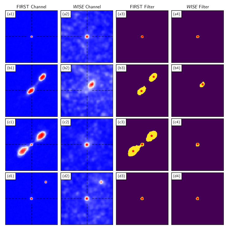
Figure 3: Example prototypes and their corresponding filters constructed by PINK belonging to neurons from Figure 14 that have been selected to demonstrate the broad set of morphologies described in §5.1. The ‘FIRST Channel’ (first) and ‘WISE Channel’ (second) columns are the FIRST and WISE channels of prototype weights selected from Figure 14. Overlaid are vertical and horizontal dash lines that denote the centre of the image. These prototypes are $3.5\mathrm{\prime }$ in angular size at the FIRST resolution. The ‘FIRST Filter’ (third) and ‘WISE Filter’ (fourth) columns show corresponding filters produced using the segmentation method described in §5.2. Denoted as red stars on each of these filters are the corresponding pixel positions obtained by the annotation process described in §5.1. The yellow islands represent the inclusion region of each filter.

A properly trained SOM should contain a representative neuron for each item in the training dataset. Therefore, labels attached to a single neuron can be transferred to any items that share this neuron as their BMU. We therefore annotated each of the $1,600$ neurons on our Layer Two SOM. We maintain a simple labelling scheme where we recorded the pixel positions of any radio and infrared features that were related to the centred radio component. Across all prototypes only a single infrared feature was annotated, since we expect that each host galaxy will have only one infrared component. We place no limit to the number of radio features that were recorded, but in practice found that three was sufficient. We tried to place annotated pixel positions at the approximate centre of each island of pixels. These only needed to be approximate positions as they are subsequently used as seeds for an island segmentation method (§5.2).

5.2 Constructing filters

The aim of this study was to identify sets of related radio components and their corresponding host galaxy within an unsupervised ML framework. To do this we first mapped each of the individual training images onto the Layer Two SOM (Figure 14) to retrieve their BMU and the corresponding $\phi$ (angle of rotation and flip flag) used to minimise Equation 4.

Next we used the pixel positions of annotated features for each neuron to craft an equivalent set of binary filters that represent arbitrary shapes based on the prototype weights constructed by PINK. We created these filters by first applying a thresholding operation to each of the prototype weights to produce a set of candidate islands. The threshold intensity was defined to be $N_{t}\times\left(I_{\mathrm{max}}-I_{\mathrm{min}}\right)+I_{\mathrm{min}}$, where $I_{\mathrm{max}}$ and $I_{\mathrm{min}}$ were the maximum and minimum pixel intensities within a channel of the prototype weights, respectively, and $N_{t}$ was initially set to $0.9$. If an island contained an annotated pixel position, it was retained, otherwise it was discarded. To the remaining islands we applied filling and dilation steps to ensure they contained no empty pixels (van der Walt et al., 2014). These remaining islands correspond to an inclusion zone. If there were fewer than $10$ pixels in the inclusion zone we repeated this procedure with $N_{t}=0.8$. In Figure 3 we show four examples of these filters, including the annotated pixel positions made against the neuron. We retain these filters as simple images that are programmatically treated as multi-dimensional arrays in subsequent processing (§ 5.3).

5.3 Mapping and filtering source components

Source catalogues represent a model of the sky as observed within some image. In a similar manner, PINK also attempts to construct prototypes that model features within an image dataset. Sharing annotated knowledge from annotated PINK neurons to a source catalogue requires a transformation between the Cartesian coordinate system of a prototype/filter to an absolute on-sky position.

To do this, consider a single radio component at some on-sky position. We first identify all nearby radio components within a $6\mathrm{\prime }$ radius. This large radius is adopted to select all components potentially within the field of view of that component’s corresponding filter after a transform has been applied. The angular offsets on the celestial sphere between the radio component position and the positions of nearby components are calculated and then converted to Cartesian pixel offsets $\left(x_{0},y_{0}\right)$ using the known FIRST resolution ($1.8\mathrm{″}$/pix). Next, the BMU of the subject radio component image is identified and the appropriate PINK derived transform $\phi$ is extracted. Based on the angle of rotation ($\theta$) and flipping flag described by $\phi$, these pixel offsets are then transformed following

$$x_{0}^{\prime} =y_{0}\times\mathrm{cos}\left(\theta\right)-x_{0}\times\mathrm{sin}\left(\theta\right)$$ (6)

$$y_{0}^{\prime} =y_{0}\times\mathrm{sin}\left(\theta\right)+x_{0}\times\mathrm{cos}\left(\theta\right),$$ (7)

and in the case where a flipping action was performed $x_{0}^{\prime}$ is negated. The positions $\left(x_{0}^{\prime},y_{0}^{\prime}\right)$ now describe nearby components in the reference frame of the BMU filter. We can therefore directly evaluate whether the components in a Cartesian frame fall within the bounds determined by the inclusion region of a filter. The corresponding nearby components whose transformed positions fell within the inclusion region were then noted as being related to the centred subject radio component. This process is carried out for both the FIRST and WISE channels, where for the WISE channel we instead search for nearby infrared sources from the AllWISE catalogue (Cutri, 2013). The use of carefully constructed shaped filters offers a large degree of flexibility to capture unique morphologies. We refer to this approach of grouping components as a ‘cookie-cutter’ method. For convenience $M_{c}$ will be used to describe sets of candidate radio components and infrared sources that passed through a subject’s filter.

We applied this cookie-cutter to all $894,415$ radio component positions in our training dataset, which produced as many as $M_{c}$ sets. For the infrared neuron we also transformed the annotated pixel position to an absolute sky position for each source. We will refer to these as ‘infrared predicted positions’. For consistency we only filter FIRST components whose images were in our training set.

5.4 Collating related source components

As each of the $894,415$ radio components in our training dataset now carry a $M_{c}$ set after being mapped to Figure 14 in isolation, we now collate these results into a catalogue of groups that describe related radio components and their corresponding infrared host. For heavily resolved radio objects represented by two or more catalogued radio components (e.g. AGN with two distinct radio lobes) there is potential for redundant information to be present among the multiple $M_{c}$ sets. Due to field of view effects and unique morphological features, often these $M_{c}$ sets may not be entirely self-consistent. This is especially true for resolved AGN with large angular separations between their radio lobes.

We adopt a straightforward method of collating this information together using graph theory (Hagberg et al., 2008). First, each of the $894,415$ radio components within our training dataset were placed as nodes on a graph. Next we sorted neurons based on the maximum distance between any two annotated click positions within the radio channel of each neuron. Sorting in this manner often placed neurons with AGNs centred on their core towards the beginning of the sorted list, and placed point sources towards the end. For neurons with a single radio position annotated, they were simply ordered by their position on the SOM (top-left to bottom-right).

Our procedure then iterated across the ordered list of neurons. For each neuron we selected all $M_{c}$ sets produced by this neuron’s filter. Given a $M_{c}$, we would work out each combination of listed radio component pairs and add an edge between their nodes on the graph. Once a node had an edge, the $M_{c}$ set produced by that component would be excluded from subsequent processing. This essentially was a greedy process, where we aimed to connect together as many nodes (i.e. radio components) together with as few $M_{c}$ sets as possible while giving preference to $M_{c}$ sets whose images were resolved radio AGN that were centred towards their host (as these neurons were processed at the earliest stages of this greedy process). When this was finished, isolated trees of nodes on this graph correspond to unique groups of related radio components within the FIRST catalogue. Each group of components was assigned a group identification (GID).

Potentially, many $M_{c}$ sets may be used for a heavily resolved radio object with many radio components. To reduce the number of AllWISE sources included in each group as potential hosts, we only select the AllWISE sources from the $M_{c}$ that contained the largest set of FIRST components. If this $M_{c}$ contained more than ten AllWISE sources (which occurred in confused fields or with an erroneously constructed filter based on a neuron with ambiguous or poorly defined infrared features) we drop all infrared host information from the collated set.

Ideally each $M_{c}$ for each collected object would contain a single infrared AllWISE source. In practice, this was not always true, as the filters may not be restrictive enough to select a single AllWISE source in all situations. We therefore assign a numerical flag (grp_flag) to each collated group, where:

1. a single AllWISE source passes through the infrared filter and it is less than $3.4\mathrm{″}$ from a FIRST component in the same group,

2. a single AllWISE source passes through the infrared filter and is further than $3.4\mathrm{″}$ from any FIRST component in the same group,

3. more than one AllWISE source passes through the infrared filter with at least one source being less than $3.4\mathrm{″}$ from a FIRST component in the same group,

4. more than one AllWISE source passes through the infrared filter and none were less than $3.4\mathrm{″}$ from a FIRST component in the same group,

5. no AllWISE sources passed through the infrared filter.

These flags are not meant to correspond to specific physical scenarios, but are instead intended to act as a potential queryable catalogue property. As we are promoting an unsupervised framework based purely on morphological information, it is foreseeable that subsequent steps could further refine infrared host selection or use this flag as a criterion during a later sample section. The $3.4\mathrm{″}$ limit was based on results later described in Figure 4 and §6.1.1.

For this study our primary aim is to demonstrate a new unsupervised ML based approach to this difficult cross-matching problem. In the future a more advanced filtering and collating method could be developed that tightly integrates these two stages together. We discuss this improvement in §7. This method of multi-wavelength cross-cataloging (and subsequent processing described below) may also be tested with appropriate simulated image data to further refine the approach and quantify its effectiveness, which may be insightful alongside measures of SOM connectivity (e.g. Tasdemir & Merényi, 2009) and subsequent analysis steps (§ 6.1.1).

5.5 Size and Curvature properties

After collating together FIRST components we derive a set of additional group properties. Given a group, $G$, that contains the FIRST radio components $F=\left[f_{0},f_{1},...,f_{n}\right]$, we calculate the maximum distance, $D$, of each group as

$$D=\mathrm{max}\left[d\left(f_{i},f_{j}\right)\right]:f_{i},f_{j}\in F,$$ (8)

where $d$ is a function to calculate the on-sky separation between components $f_{i}$ and $f_{j}$. This was performed as an exhaustive search between all combinations of two components and was only possible for groups with two or more FIRST components. This gives a robust estimation of the projected angular size of all groups that we have collated together. As prototypes are generalised representations of predominate morphologies, simply transferring a an angular distance from an annotated neuron to an individual object may not be ideal.

With the set of components for each group and the corresponding pair of components with the largest distance ($f_{i}$ and $f_{j}$) in that $G$, we can calculate a ratio to identify curved or morphologically disturbed objects. We measure the shortest path, $SP$, by finding the optimal order to $F$ such that

$$SP=\mathrm{min}\left(\sum_{k=0}^{n}d(f_{k},f_{k+1})\right):f_{i}=f_{0},f_{j}=f_{n}.$$ (9)

These two competing quantities can be used to defined a ‘curliness factor’ ($Q$), which is simply,

$$Q=\frac{SP}{D}.$$ (10)

For groups with only two FIRST components, $Q$ will evaluated to be 1. However, for groups with three or more components, the $Q$ will be high for instances where components are not in a straight line (e.g. bent-tail AGN). This $Q$ statistic would be a lower limit for extremely bent AGN where the radio lobes are closer together than they are to the host position.

6 Results

6.1 Assessing AllWISE Source Matches

Using a dimensionality reduction technique, we have created a set of $1,600$ representative galaxy morphologies at radio and infrared wavelengths. Combining this with a simple annotation scheme and pixel intensity thresholding, a corresponding set of filters were created. These filters were then projected through catalogue space to identify sets of related components. As we have no training labels, it is difficult to establish and quote accuracy, reliability and purity measures that are often used in supervised learning contexts for the same problem (Lukic et al., 2018; Alger et al., 2018; Wu et al., 2019).

As an alternative, the approach we adopt is to use the predicted positions (absolute sky positions based on transformed annotated pixel positions) and perform nearest-neighbour searches against genuine and randomised catalogues. Although this may lose spatial information maintained by the filters, conceptually it is similar to other metrics already used through the literature (e.g. Downes et al., 1986). We pursue this approach throughout this study to assess reliability. Practically it is straight forward to implement with minimal computation cost and should be accurate as annotated positions were recorded at the centre of important features.

6.1.1 Cross-matching infrared predicted positions

We now assess the usability of the infrared host identified for each collated group. The source sky-density of WISE is $\sim$15\,000\text{\,}\deg^{-2}$$ and is higher than FIRST’s by a factor $\sim 200$, making this aspect of the collation problem more difficult. We first cross-referenced our infrared predicted positions to the AllWISE catalogue (Cutri, 2013). We searched for all AllWISE sources $<$$$ of these positions. To establish the by-chance coincidence rate of a foreground or background AllWISE source at any arbitrary position we performed a Monte-Carlo test where we created a ‘shifted’ predicted position catalogue by adding a constant $3\mathrm{\prime }$ offset to the declination to the genuine set of infrared predicted positions.

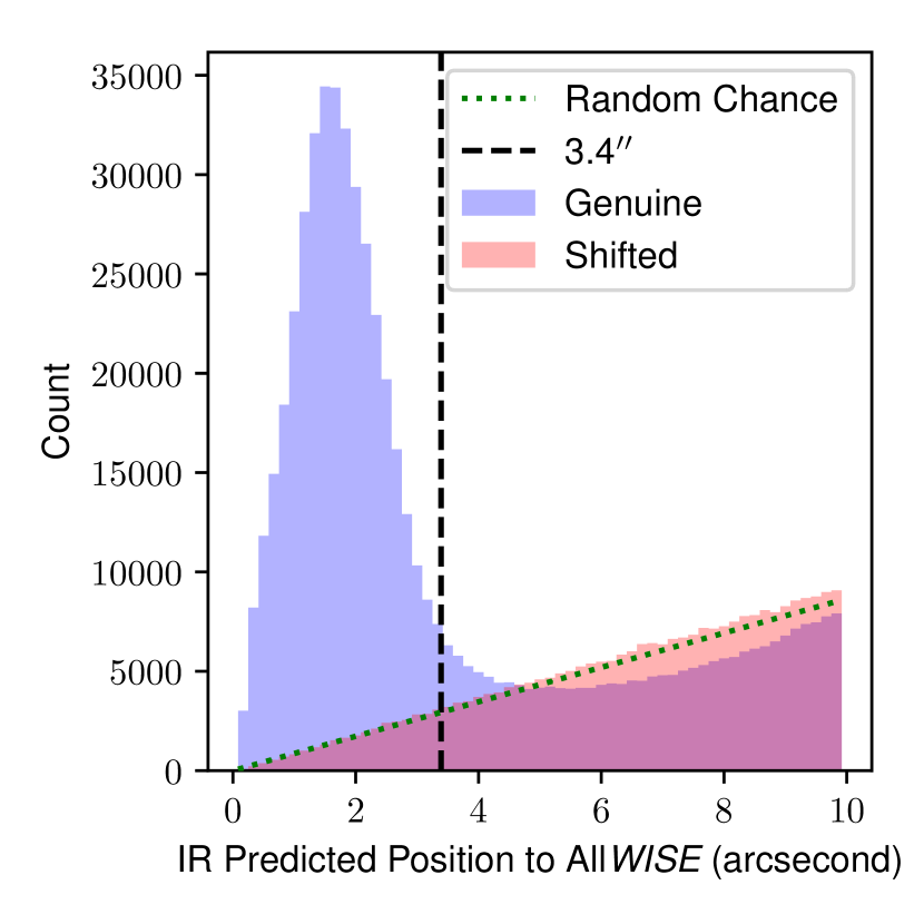
Figure 4: The number of AllWISE objects found in 60 annuli evenly spaced between $0-$$$ for positions described in a genuine and shifted catalogues. This was performed only for groups with a single FIRST component (i.e. point sources). Overlaid as the green dotted curve is the chance alignment rate described by Equation 11. The vertical dash-dash line shows the point where the genuine catalogue has double the number of sources than the shifted catalogue, which we calculate to be at $3.4\mathrm{″}$.

Next we construct 60 annuli evenly spaced between $0-$$$ around each position in the genuine and shifted infrared host catalogues and count the number of returned matches. These counts for groups with a single collated FIRST radio component are presented in Figure 4. For the shifted catalogue positions, the number of returned AllWISE sources is proportional to the area within each annulus. This establishes the chance coincidence rate of foreground or background objects with respect to some arbitrary position. The genuine catalogue has $351,310$ more AllWISE counterparts $<$$$ than the shifted catalogue. By assuming the source density of AllWISE to be $\rho_{0}\sim$$15\,000\text{\,}\deg^{-2}$ and uniform across the segmented area, the chance count, $B$, of a foreground or background object being present between offsets of $r$ and $r+dr$ can be formulated as,

$$B=N\rho_{0}\left(2\pi r\right)dr,$$ (11)

where $N$ corresponds to the number of positions searched around. Overlaying Equation 11 onto Figure 4 shows that it agrees with the object counts of the shifted catalogue.

We find that, at an offset of $3.4\mathrm{″}$, the number of sources in the genuine infrared predicted position catalogue is twice the number of the shifted infrared predicted position catalogue. At this radius the likelihood of there being a genuine match for a predicted host position is about the same as random chance.

Following Ching et al. (2017), a measure of reliability, $R$, of a cross-matched catalogue can be established by,

$$R=1-N_{\mathrm{shift}}^{\mathrm{match}}/N_{\mathrm{genuine}}^{\mathrm{match}},$$ (12)

where $N_{\mathrm{shift}}^{\mathrm{match}}$ and $N_{\mathrm{genuine}}^{\mathrm{match}}$ are the number of matches found between some target catalogue and the set of shifted (i.e., random) and genuine catalogues, respectively. Given Figure 4, at $3.4\mathrm{″}$ the $R$ statistic is $\sim 92.5$%, and improves as the offset distance becomes closer to zero. Ching et al. (2017) provided optical identifications using data from Sloan digital sky survey (SDSS) of $19,179$ of radio sources from FIRST using over an area of $800\text{\,}\deg^{2}$. They obtain a reliability of $93.5$% using a rule-based methodology with visualisation inspection of complex FIRST sources.

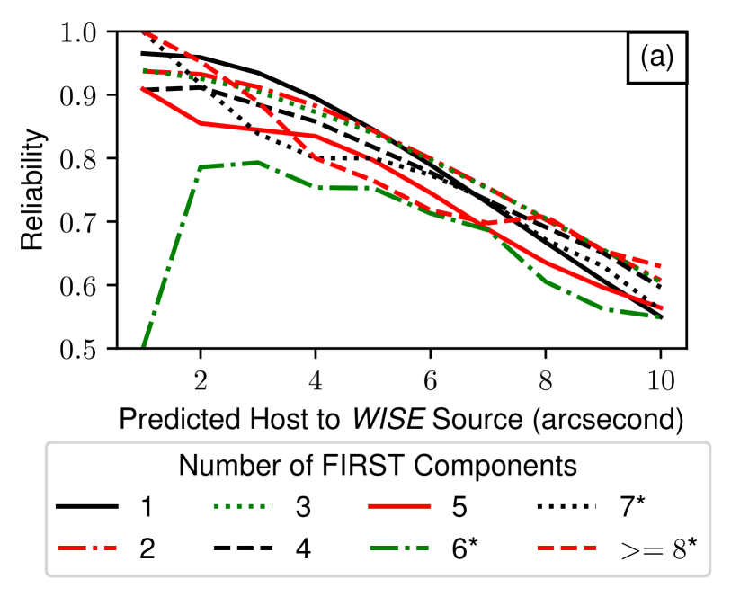
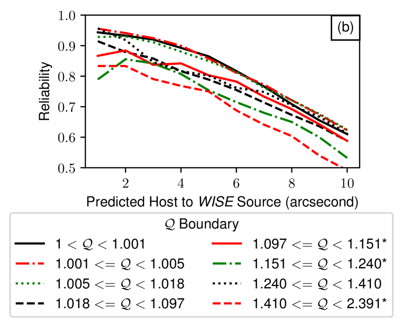
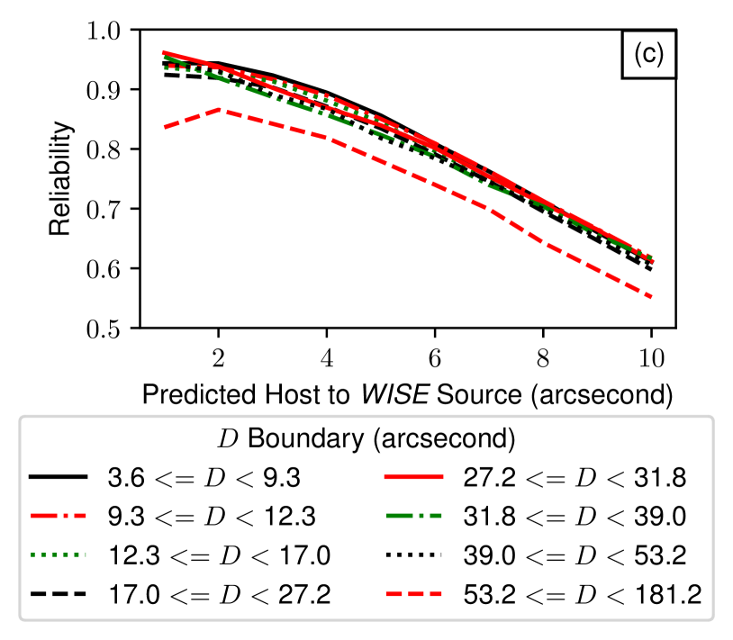
Figure 5: (a) The reliability curves of the cross-matched infrared predicted positions against AllWISE as a function of number of collated FIRST components. (b) The reliability curves of the cross-matched infrared predicted positions made against AllWISE as a function of the $\mathcal{Q}$ parameter. Boundaries of the $\mathcal{Q}$ were spaced to contain roughly the same number of groups to maximise the clarity of the different reliability trends. All groups included in this figure contain three or more FIRST components. (c) The same as (b) except as a function of $D$. All groups included in this figure contain two or more FIRST components. Labels with a ‘*’-suffix denote categories with fewer than 15 genuine matches with separations $<$$$.

We generalise this analysis to all collated groups and investigate any second order effects as functions of collated number of FIRST components, maximum distance ($D$) and curliness ($Q$). The $R$ was evaluated across a range of separations (spaced from $0-$$$ in steps of $1\mathrm{″}$) after dividing our collated groups into meaningful subsets. For the subsets in the $D$ and $Q$ dimensions we established boundaries at the 20^th, 40^th, 60^th, 80^th, 85^th, 90^th and 95^th percentiles, where finer bins were used in regions of the parameter space with rapid variations identified after inspection the distribution. Otherwise we created boundaries based on the number of associated FIRST components in each collated group. We interpolate between $R$ measures across these dimensions to create a set of reliability curves, which we present as Figure 5. Broadly speaking these curves show that as measures of complexity increase, judged either by the number of collated FIRST components or $Q$, the infrared predicted position becomes less reliable. At a threshold of $3.4\mathrm{″}$ these $R$ are above 80% with significant spreads of upwards of $\sim 12$% between the simple and complex groups. However, the reliability curves in Figure 5c suggest groups across all $D$ have about the same degree of reliability. We use these interpolated reliability curves to provide a measure of reliability for all collated groups in our catalogue data products for each of these dimensions. For groups outside the range of these reliability curves we set the $R=0.5$ across all dimensions. Six of the 24 reliability curves in Figure 5 have fewer than 20 genuine matches with separations $<$$$ and are the most susceptible to small number statistical effects. Since increasing separations accumulate counts from smaller separations (i.e. bins are not exclusive), the number of genuine matches very quickly grows so that all other curves and separation bins have at least twenty genuine matches.

We highlight that assessing reliability in this manner may be incomplete as it is only testing for the presence of an infrared source near a specific position, and not necessarily testing the relationship between the radio and infrared characteristics of a subject galaxy. Given that the neuron prototype weights are constructed to represent features within an image, it is not surprising that there will often be a infrared source at our predicted positions. It would be interesting to repeat this procedure after removing the infrared channel from the pre-processed images and Figure 14 to assess its influence. However, we suspect that without the infrared information available the determination of the host position given just radio information will be less reliable because the nature of the radio emission becomes ambiguous. Also, our infrared predicted position are ultimately tied to the selection of a BMU, which in-of-itself may be perturbed by a spurious infrared source in a subject image. In such cases using multiple neurons to recognise conflicting information or a more robust collation procedure may be required to produce a more physically reliable classification. Invoking alternative SOM statistics (e.g. Tasdemir & Merényi, 2009) could also be useful in detecting and handling ambiguity within the cookie-cutter and subsequent collation process.

6.2 Description of Catalogues

We present two catalogues that have been produced using our ‘cookie-cutter’ approach to grouping and host identification.

The first catalogue we present is based on the FIRST catalogue, but is supplemented with additional columns of information. It details the $894,390$ radio components whose FIRST and WISE images were successfully downloaded, preprocessed and included in our training dataset (Table 1). We provide all information from the FIRST catalogue related to the properties of the radio components themselves (not value added information from earlier cross-matching). As additional columns we include PINK provided data products, including the BMU position upon the SOM lattice, Euclidean distance to the BMU, and transformation parameters derived by Equation 4. These BMU and transform information could be applied to other image datasets directly if the layout of our Layer Two SOM is accepted. For each radio component we also include a GID to distinguish unique collated groups of related radio components. We will refer to this as the FIRST supplemented catalogue (FSC).

As a second separate catalogue we describe properties of each of the $802,646$ collated groups we have identified. For each group we supply an appropriate GID to identify the related FIRST radio components from our FSC. Included are the solutions to Equations 8, 9 and 10. In column D_idx we present a comma-separated tuple detailing the indices of the FIRST components in the FSC that solved Equation 8. A similar column titled SP_idx contains comma separated tuples that highlight the order of FIRST components visited when solving Equation 9. Note here that the path will start and end on the sources described in the D_idx components. Reliability measures for each collated group as functions of $Q$, number of collated FIRST components and maximum component separations are also included. As the column comp_host we provide a comma-separated tuple that includes the names of any AllWISE sources that passed through the infrared filter. Of these sources, our prob_host contains the AllWISE source name of the source closest to any FIRST component in the same group if the on-sky separation is less than $3.4\mathrm{″}$. The infrared predicted position, that were used for the reliability analysis, are also included. We refer to this as the group reference catalogue (GRC) and provide a concise summary of columns in both the FSC and GRC in Table 3 and also include a five-row extract of each in Appendix B.

Column	Description
FIRST Supplemented Catalogue
GID	The unique identifier for each group
idx	A unique identifier for each FIRST radio component
neuron_index	A three element tuple containing the index of the BMU for the image corresponding to this FIRST component position
ED	The Euclidean distance between the transformed image and the BMU
flip	Whether the image was flipped to align with the BMU
rotation	The angle of rotation that the input image was rotated to align with the BMU, in radians
Group Reference Catalogue
GID	The unique identifier for each group
prob_host	AllWISE source name of the probable host
comp_host	Names of any AllWISE sources that also passed through the infrared filter
grp_flag	The set of flags described in §5.4
D_idx	The indices of the FIRST components with the largest angular separation
D	The distance $D$ in arcseconds
SP_idx	List of indices of FIRST components that produce $SP$
SP	Length of the shortest path in arcseconds
Q	The $Q$ factor
rel_g	Approximate reliability as a function of number of collated FIRST components
rel_Q	Approximate reliability as a function of $Q$
rel_D	Approximate reliability as a function of $D$
ir_pp_ra	The RA of the infrared predicted position in degrees
ir_pp_dec	The Dec of the infrared predicted position in degrees

Table 3: A description of the columns that make up the catalogues our method of source collation have produced. The units for each column are dimensionless unless specified otherwise.

We present in Figure 6 the distribution of the number of FIRST components collated and their occurrence. As expected, the overwhelming majority (about 732,000) are groups with a size of one. These correspond to either point source objects, which remain unresolved at the FIRST resolution, or slightly resolved objects that are characterised well by a single two-dimensional Gaussian. Cross-referencing these point sources to other surveys is largely a simple task that can be achieved with a straight-forward nearest neighbour search (Norris et al., 2011). Resolved objects with many radio components represent the situations where the simple nearest neighbour approach to cross-matching often fails, as these resolved radio components are potentially separated from one another and their host galaxy (Banfield et al., 2015; Alger et al., 2018). In 62% of these groups, at least one AllWISE source has been listed as a competing host.

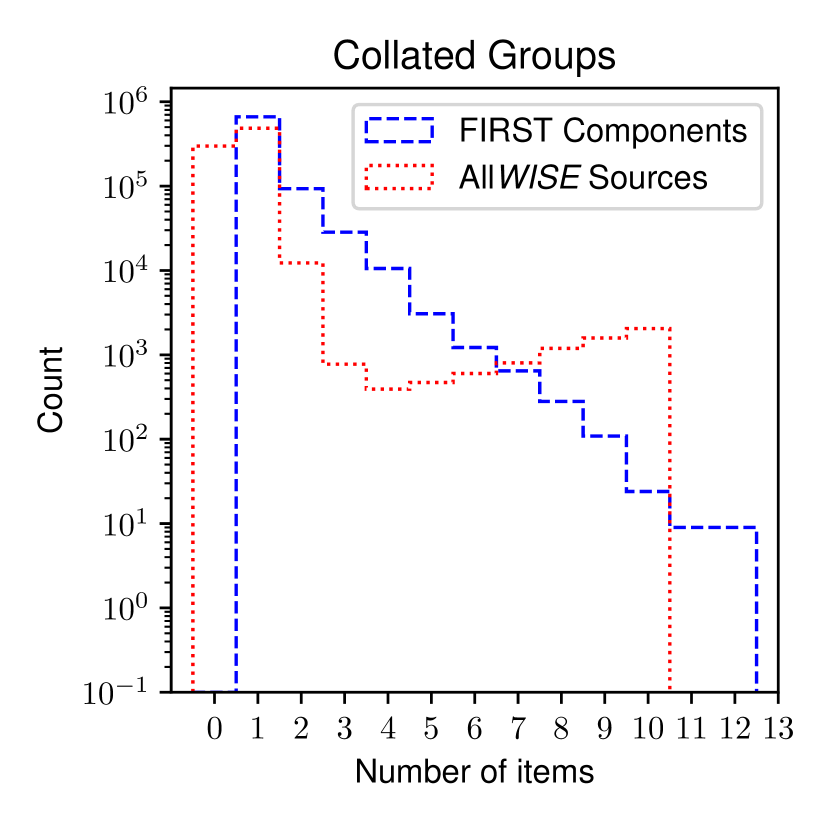
Figure 6: Distribution of the number of FIRST components and potential AllWISE host sources associated with each collated group.

6.3 Outlying sources

The data deluge from future all-sky radio continuum surveys requires an approach of intelligently assigning meaningful objects to expert users for inspection, whose time and effort should be considered a scarce resource. To maximise the scientific impact, objects presented to human classifiers should be exceptionally rare, interesting and unexpected (Crawford et al., 2017; Norris, 2017b). Further, it will likely be on these exceptional objects that most classification algorithms, no matter their sophistication, will struggle to perform reliably.

Assuming an adequately trained map, predominant features in the training dataset should have a representative neuron upon the SOM lattice. We examined the distribution of Euclidean distances (Equation 4) of all $894,415$ objects in our training dataset and found it to follow a log-normal distribution with a mean and standard deviation of 15.3 and 12.9, respectively. We could consider a mapping to be ‘good’ if its euclidean distance is less than $+1\sigma$ from the mean (i.e. $<28.2$).

Selecting sources based on their distance from the PINK produced prototypes would be an obvious method of segmenting small sets of objects from a larger dataset. To highlight how this measure can be mined for rare and exceptional objects, we show in Figure 7 the eight positions whose mapping to our SOM produced the largest set of Euclidean distances (Equation 4), and provide a brief overview of their significance. These objects were not intentionally selected or curated, and are presented to demonstrate that segmenting outliers in this manner is an effective tool capable of isolating physically interesting objects that are in active areas of research.

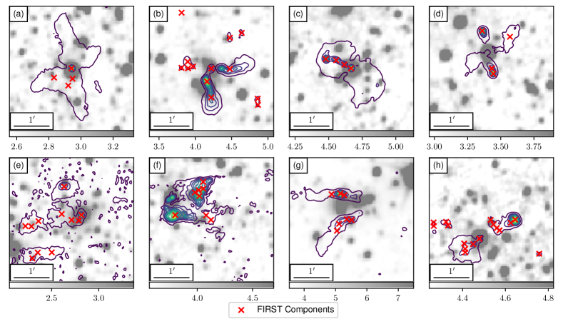
Figure 7: Positions centred towards the FIRST radio components with the worst Euclidean distance calculated by PINK out of the entire training dataset. The grayscale images and corresponding colourbar are the WISE $W1$ band image towards these positions, with pixel intensities in units of DN. Colour contours represented 12 levels of intensity that are evenly spaced between $0.25\sigma$ to the maximum intensity of the FIRST image. Note that we are not highlighting the results of our collation procedure and are simply overlaying FIRST components.

From the eight images we highlight in Figure 7 as outliers, panels (a) and (d) have clear X-shaped radio features. So called ‘X-shaped’ resolved radio galaxies are an ongoing and active area of research (Leahy & Williams, 1984; Dennett-Thorpe et al., 2002; Capetti et al., 2002; Cheung, 2007; Cheung et al., 2009; Saripalli & Subrahmanyan, 2009; Saripalli & Roberts, 2018; Yang et al., 2019). These are a set of objects in which there is an additional pair of low surface brightness wings of emission at an angle to the active set of radio lobes (Cheung, 2007). The origin of this secondary set of wings is undecided, but common scenarios describe a blackflow of plasma from the set of active lobes, or the rapid realignment of jets, possibly after the merger of two black holes. Yang et al. (2019) recently examined a recent version of the FIRST catalogue and identified 290 X-shaped radio sources, 184 of which being labeled as ‘probable’, making them a fairly rare morphological feature. Our two X-shaped radio galaxies are among their sample.

Hybrid morphology radio sources (HyMoRS) are a class of objects that exhibit different Fanaroff-Riley (FR) classes on opposite sides of their nuclei (Fanaroff & Riley, 1974). There is ongoing discussion about the mechanism that causes these different morphological structures and whether their manifestation is a symptom of an environmental (nurture) or intrinsic (nature) condition (Kapińska et al., 2017). Building statistically significant samples presents an opportunity towards understanding conditions of this nurture versus nature debate. The radio sources in Panels (c) and (h) of Figure 7 exhibit HyMoRS-like morphologies.

Panels (b), (f) and (g) of Figure 7 exhibit bent-tail (BT) radio morphologies, sometimes referred to as wide-angle tails and narrow-angle tails, with their radio lobes appearing to bend away from their typical linear trajectory toward a common direction (Mao et al., 2010; O’Brien et al., 2018). BTs have often been used as tracers of cluster and dense inter-galactic medium (IGM) regions, as their jets are bent by ram pressure applied from the relative motion of its host galaxy moving through a dense medium.

Finally, panel (e) shows a set of radio contours that are highly disturbed and irregular. Even with the inclusion of AllWISE information it is unclear whether these radio components are all related to a single intrinsic object or many distinct objects in close proximity. This region was also presented as figure 7 of Banfield et al. (2015) as an example of unusual structures that have been identified by citizen scientists participating in RGZ. We emphasis that Figure 7 was based on information from an entirely unsupervised ML algorithm without curation. This coincidence further highlights the capability of segmenting interesting objects from a larger dataset using this parameter space.

6.4 Groups of Radio Sources

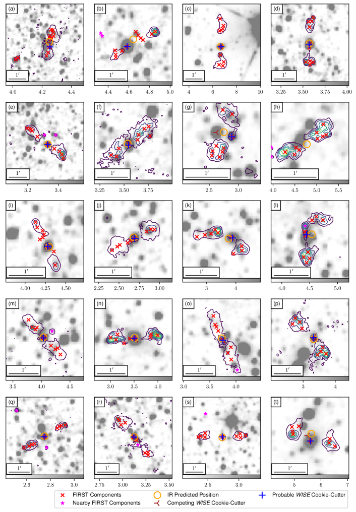
Figure 8: The twenty collated groups with the largest collection of FIRST components. For each panel the grayscale image and corresponding colour bar represent the WISE $W1$ image, with pixel intensities in unit of DN. FIRST radio components with the target GID are labelled as ‘FIRST components’ whereas components with an unrelated GID are ‘Nearby FIRST Components’. Any AllWISE source that passed through the projected filter are labelled as ‘Competing WISE Cookie-Cutter’, and of these sources (if any), we label the one closest to a FIRST component as ‘Probable WISE Cookie-Cutter’ if it was within $3.4\mathrm{″}$ (§5.4). The ‘IR Predicted Position’ describes the annotated infrared pixel position after being transformed to an absolute sky position. Colour contours are six levels evenly spaced between $0.5\sigma$ to the maximum intensity and are based on the FIRST image.

To highlight the structures recovered from our method, we show in Figure 8 the twenty groups with the largest set of collated FIRST components. From these examples a number of points can be made. The most obvious is that applying the BMU filters to the FIRST components as a selection tool has recovered meaningful relationships that extend beyond simple islands of contiguous pixels. Seven of the example groups have radio lobes that are separated from their presumed host by angular distances $>$$$. Immediately this extends the capabilities of modern source finders which can include island information for decomposed radio components (Mohan & Rafferty, 2015; Hancock et al., 2018; Robotham et al., 2018).

Secondly, projecting meaningfully constructed filters through the catalogue space (the ‘cookie-cutter’ procedure) has performed remarkably well at separating unrelated source features from one another. Images in panels (b), (e), (h), (m) and (q) of Figure 8 demonstrate instances where nearby FIRST components have not been associated with the target group despite being in relatively close proximity ($<$$$) to some of their resolved components. In contrast, panels (l) and (r) show cases where there are unassociated FIRST components that could reasonably be grouped with the target collated group. Including island information from modern source finding codes process may help for these cases, as there is an additional queryable parameter linking (presumably) related radio components together.

We draw attention to panel (a) of Figure 8, which shows an AGN roughly $2\mathrm{\prime }$ in angular scale that has had two FIRST components (located towards the South-West region of the panel) incorrectly associated with it. This incorrect grouping is caused by the $3.5\mathrm{\prime }$ field of view of our neurons. When images centred on these two FIRST components were mapped onto our SOM, PINK only had visibility of the southern AGN lobe (and not the northern lobe). By chance there was also an infrared source located roughly between these two radio components and the southern lobe. Hence, PINK’s similarity measure responded well to prototypes corresponding to AGN radio morphologies. Our present approach of collating results together only considers the BMU mapping of each component in isolation and does not attempt to verify a self-consistent sky-model. We discuss potential improvements to address these scenarios in §7.

The infrared sky as surveyed by WISE has a high source density ($15\,000\text{\,}\deg^{-2}$) and is beginning to approach its source confusion limit. Our approach of projecting an appropriately derived filter through catalogue space does a reasonable job of selecting candidate host objects from the AllWISE catalogue. In some cases, such as panels (a), (f), (g), (m), (n), (p) and (t), these filters have captured more than one AllWISE source. These tend to be in especially confused fields. Where possible, we break this degeneracy by relying upon one of these host candidates being coincident with a FIRST radio component. Otherwise, for the remaining panels, with the exception of (h), an AllWISE source has been identified by passing unaccompanied through the projected filter.

During this stage we also highlight the sky position obtained by transforming the annotated pixel position made against the infrared channel of the prototype weights for panels in Figure 8. These are denoted as ‘IR Predicted Position’ and often are aligned closely to the captured AllWISE hosts. We include these transformed feature locations to argue that our reliability assessment (§6.1.1) is an appropriate first order approximation of our overall ‘cookie-cutter’ methodology. For cases where no AllWISE sources passed through the appropriate filter, searching around this transformed infrared feature location in a nearest neighbour type fashion may itself be an effective method if locating a probable infrared host galaxy.

We manually inspected a set of 200 groups (sorted in a descending order by the number of FIRST components) and find that these presented examples are representative. However, $\sim 20\%$ of heavily resolved objects with extremely bent radio lobes had an incorrect of misaligned predicted infrared host.

6.5 Curved Sources

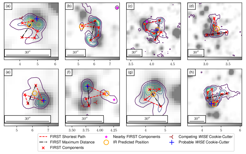
Figure 9: A set of eight groups with the largest $Q$ factors. Legend items carry the same meaning as Figure 8, except we include as the dot-dash black line we show the pair of FIRST components with the maximum separation (Equation 8), and as the dash-dash red line we show the corresponding shortest path (Equation 9). Colour contours represent six intensity levels evenly spaced between $2\sigma$ and the maximum intensity of the FIRST image.

We derived the $Q$ statistic (Equation 10) after examining the prototypes constructed by PINK and noticing that there were few neurons that exhibit clear radio lobes with disturbed and bent morphologies. Instead, prototypes were constructed to have very circular lobes with the practical effect of matching to any radio morphology with bent lobes. As a consequence, individual images of actual BT radio objects had unreasonable infrared sources presented as likely hosts. Therefore, crafting some measure of ‘curliness’ would be a useful quantity to (i) identify these interesting objects with bent morphologies, and (ii) include a metric that would suggest that our potential infrared hosts and their associated FIRST components are not as reliable as a more typical object.

We show the eight collated groups with the largest $Q$ statistic from our GRC in Figure LABEL:fig:curl. A set of general impressions can be drawn from these example groups. The first is this $Q$ statistic is successful in extracting a set of groups that would be considered to be BT objects, panels (a), (c), (d), (f), (g) and (h), depending on the definition adopted. Compared to the objects from Figure 7, the groups with high $Q$ values are generally much smaller in angular scales, with all being $<$$$.

Visually inspecting these eight (and other) high $Q$ groups reveals that our cookie-cutter method has sometimes allowed more than a single AllWISE source to pass through the projected infrared filter and present as a potential host. Many of these are not believable candidates and are an artefact of a misapplied filter made against an under-represented galaxy morphology. To some degree, searching for coincident FIRST radio components has helped to reduce this competing set of infrared sources to a more compelling host - a criteria we describe in §5.4. Panels (a) and (f) illustrate this, as both have at least two AllWISE sources nominated as potential hosts. However, for these examples a reasonable AllWISE source has been selected based on its proximity to a corresponding collated FIRST component.

Included in each panel of Figure LABEL:fig:curl are the infrared predicted positions. Comparing these to the set of AllWISE sources nominated as potential hosts the projection of a filter through catalogue space highlights how there can be significant disagreement between the two approaches. In cases where no AllWISE sources passed through a filter, the infrared predicted positions generally lies towards the geometric mean of all grouped FIRST components, not towards the ‘root’ of both jets. This could be thought of as a natural consequence of these types of objects being under-represented with appropriate neurons on the lattice, and an over-generalisation of the few neurons that attempt to characterise their unique shapes. We discuss potential avenues of improvement in §7 for these class of objects.

6.6 Identification of GRGs

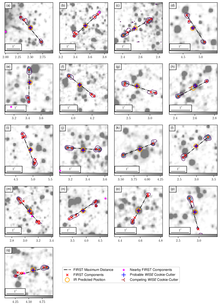
Figure 10: The 17 GRGs we have found from the FIRST survey using our method of component collation. Legend items, images and contours carry the same meaning as Figure 8, except we include as the dot-dash black line we show the pair of FIRST components with the maximum separation (Equation 8) that were used to obtain a physical size.

Another scientific outcome from our compiled GRC is the search for Giant Radio Galaxies. GRG are radio sources with physical sizes exceeding $0.7\text{\,}\mathrm{Mpc}$ (Dabhade et al., 2017), making them among the largest individual astronomical objects in the Universe. It is thought that their immense radio lobes are powered by an accreting super massive black hole (SMBH) of mass between $10^{8}$-$10^{10}$ M_⊙ (Lynden-Bell, 1969; Begelman et al., 1984). However, the mechanism that allows their radio jets grow to these extreme physical scales is debatable. One scenario is that the matter surrounding the GRG, the IGM, has a low density, thereby allowing the jets to grow without being confined or frustrated (Jamrozy et al., 2008; Subrahmanyan et al., 2008; Safouris et al., 2009; Malarecki et al., 2015). Alternatively, GRG could simply be an older population of typical radio galaxies that have grown to their current size over long time-scales (Kaiser et al., 1997). Building sufficiently large samples of GRG that can begin to distinguish these scenarios is difficult due to their rarity. Mining all-sky radio-continuum surveys for GRG are one of the most efficient methods of locating them (Dabhade et al., 2017, 2019). The task of identifying related radio lobes is only a single component of searching for GRG, with the more difficult being host galaxy identification. Our collation method and resulting catalogue set contains this information.

We search for GRG in our GRC by first selecting groups with

1. a grp_flag of either ‘1’ or ‘3’, and

2. a D greater than zero.

Item 1 describes sources where an AllWISE passed through the projected filter and was coincident with to within $<$$$ of a FIRST component in the same collated set. This criteria selects radio objects where our collation method has identified a likely infrared host. The secondary criteria 2 ensures only resolved objects with a measurable angular extent are returned.

Applying these criteria reduced the set of $802,646$ groups in our GRC to $19,539$. To obtain a distance measure to the host object we search for spectroscopic redshifts of the $19,539$ AllWISE sources from two SDSS catalogues. Our primary catalogue was from Pâris et al. (2017), who describe spectra of $297,301$ visually confirmed quasars from the Baryon Oscillation Spectroscopic Survey (BOSS) from SDSS. Our secondary catalogue was SDSS data release 12 (Alam et al., 2015), which contained upwards of 470 million spectra. We place preferences towards matches made against Pâris et al. (2017) as their pipeline was tailored towards the broad-line emission and absorption features that are typical of quasar optical spectra that the SDSS pipeline has difficulty with. Matches for $13,931$ of the $19,539$ sources were found within a $3.25\mathrm{″}$ radius, $4,337$ of which possessed a spectroscopic redshift. Cross-matching was performed using the X-Match remote service from CDS. Although there are newer SDSS data releases (Albareti et al., 2017; Abolfathi et al., 2018; Aguado et al., 2019), they are not yet available through the X-Match interface.

We then calculated the proper physical size of these $4,337$ sources, accounting for the apparent change in angular scale of objects at cosmologically significant distances (Hogg, 1999). Adopting a GRG definition of $>$0.7\text{\,}\mathrm{Mpc}$$ we identify a set of 17 GRG.

We present as Figure 10 images of these 17 GRG and outline their properties in Table 3. Included are their redshifts from SDSS, their derived physical sizes and the separation between the AllWISE source we label as the host and the cross-matched SDSS source. All of these separations are $<$$$. As we use the maximum distance between grouped radio components and not the maximum distance between resolved extended emission, their prescribed angular and physical sizes depend on the reliability of the source finding software used by FIRST, and in some cases could be considered as lower limits.

Panel	GID	SDSS	Offset	Angular	$z_{\mathrm{spec}}$	Physical
		DR12		Size		Size
			(′′)	(′′)		(kpc)
a	7	J160953.42+433411.4	0.06	142.7	0.76	1069.2
b	10	J085743.54+394528.7	0.49	151.3	0.53	964.7
c	16	J151903.65+315008.6	0.33	143.5	0.56	941.3
d	181	J111215.45+112919.2	0.33	108.5	1.13	907.5
e	259	J031413.72-075023.7	0.04	106.0	1.25	901.1
f	25	J100550.63+211652.7	0.32	131.8	0.56	862.2
g	4	J125142.03+503424.6	0.22	131.3	0.55	853.7
h	62	J103050.90+531028.7	0.03	100.3	1.20	847.1
i	31	J100751.16+165243.3	0.31	135.2	0.49	824.5
j	373	J120821.99+221958.1	0.09	108.9	0.74	809.9
k	463	J121431.15+182815.0	0.13	89.8	1.59	776.3
l	19	J161502.40+285819.0	0.36	134.8	0.43	769.4
m	12	J105224.06+373004.5	0.10	143.9	0.37	751.7
n	183	J155140.30+103548.6	0.41	143.9	0.37	741.8
o	185	J123604.51+103449.2	0.11	102.1	0.67	726.2
p	453	J131524.33+383044.1	0.29	107.1	0.59	719.1
q	465	J102215.04+174648.9	0.09	111.0	0.53	706.0

Table 4: The 17 GRG we have identified after cross-matching WISE sources to Pâris et al. (2017) and Alam et al. (2015), ordered by their proper physical size. The ‘SDSS DR12’ and ‘Offset’ columns contain the name of the nearest SDSS object name and the corresponding separation when cross-matching the infrared host objects of selected groups. The angular size is the maximum distance found following Equation 8 for each group. We include the spectroscopic redshift ($z_{\mathrm{spec}}$) provided by SDSS. Note that by chance all these objects contain redshifts are from Alam et al. (2015). The physical size has been calculated using astropy.cosmology machinery and is in units of kpc.

Provided that the redshifts from Alam et al. (2015) and Pâris et al. (2017) are reliable, these 17 GRG are likely genuine. Each of the matched AllWISE sources have an angular offset to their SDSS source that is $<$$$, making them fairly robust. To estimate the false match rate of these AllWISE sources we shifted all $19,539$ positions submitted to X-Match by $3\mathrm{\prime }$ in declination. Of these submitted sources there were only $1,301$ matches, only 7 of which possessed a spectroscopic redshift. We can therefore estimate that there is about a 1 in 200 rate ($7/1,301=0.5$%) of a spurious object entering our sample before our GRG criteria is applied. Of course, erroneous collated groups could be produced from mis-applied filters. Visually inspecting these 17 GRG suggests many are legitimate and reliable groupings, although the host galaxy selected for panel (m) may be slightly ambiguous.

We compared our catalogue to other studies (Dabhade et al., 2017, 2019), and to our knowledge 16 of these 17 GRG are previously unidentified. Dabhade et al. (2019) use data from the LOFAR Two-metre Sky Survey (LoTSS) data release one (Shimwell et al., 2019) to identify 240 GRG in a $400\text{\,}\deg^{2}$ region, and also identified the GRG we label as panel (g). In principle we could perhaps identify a larger sample of GRG by expanding our criteria to include (i) photometric redshifts available from SDSS, and (ii) groups where a single AllWISE source passed through the infrared filter but did not coincide with a collated FIRST radio component. For this study we wish to primarily publish our collation method. Instead we will leave a more thorough extraction and analysis of a GRG sample as future work.

7 Discussion and Future Outlook

Our primary focus throughout this study was to present a new approach to the source collation problem with an emphasis towards exploiting unsupervised ML algorithms. Our preliminary results based on our proof-of-concept design have produced a set of catalogues with value added data products which we have used to identify (i) rare and interesting sources, (ii) complex AGN (including the introduction of a statistic to search for AGN with curved or disturbed morphologies) and (iii) identification of 17 GRG. Below we discuss current limitations of our preliminary framework and future directions to improve its known shortcomings.

7.1 Constructing the ‘Sky-Model’

Any image or catalogue is a model of the sky-brightness observed at a particular wavelength. For simplicity when producing a catalogue describing unique groups, we treat the cookie-cutter segmentation and the collation of their results as two distinctly separate process. However, revising our implementation to tightly integrate these stages together could help produce a more self-consistent sky-model. Consider the pair of FIRST components that were incorrectly associated with the larger AGN in Figure 8a. This scenario ultimately failed as our the field of view of our neurons were too small. Presently we only consider the BMU of each mapped image. The notion of a BMU in this context can be expanded to also consider the validity of information obtained from the cookie-cutter and its consistency with the current sky-model. Sets of individual mappings could be treated as an ensemble voting upon associating sets of components together. This would likely reveal inconsistencies for situations like Figure 8a, as the many genuine components of the AGN would consistently discriminate against the two outlying FIRST components that were incorrectly associated. By detecting this disagreement the problematic voting members could have their mapped BMU replaced with another neuron with a comparable (but larger) Euclidean distance.

Alternatively, all the neurons could be used to form a crude ensemble type method, similar to a random forest classifier. Mapping a single image to each prototype and the corresponding filter would produce a set of $M_{c}$. These could collectively be weighted by the Euclidean distance that accompanies each mapping. As each neuron has the same field of view, the individual components that make up each $M_{c}$ would be the same. Therefore, the position of each component within all filters could be considered, and when weighted by the Euclidean distance of all mappings a regressed like probability score could be constructed. Placing a minimum threshold on this value would either include or exclude a component or source from membership of a group.

Our procedure attempts to expose the underlying distribution of galaxy morphologies in an accessible manner. Leveraging this allows for each step of our methodology to be understood and improved upon outside of a blackbox, which is in stark contrast to some supervised ML approaches. This may be more desirable for users who can begin to introduce domain knowledge in a more tractable way. For instance, criteria of the expected WISE colour-colour properties of AGN cores could be supplied as a property to consider when applying the cookie-cutter for filters with AGN morphologies. Such steps can be introduced in a modular fashion without the need to retrain previous steps.

7.2 Probability Treatment of Neuron Features

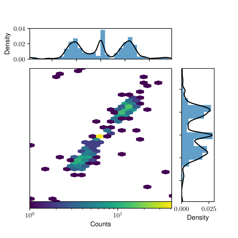
Figure 11: The two dimensional distribution of FIRST sources accumulated as they passed through the radio filter of a single neuron. The radio neuron was selected to contain a remanent of the VLA PSF. Empty hexagonal bins have been masked out. The vertical and horizontal histograms show the normalised density distribution after marginalising across the corresponding axis. Overlaid onto each the result of a kernel density estimator.

Neurons and their prototype weights could be likened as something that approximates some underlying two-dimensional probability density function (PDF) of predominant object morphologies. Prototypes are constructed in a manner similar to a weighted averaging process, so the distribution of pixel intensities across the prototype weights could be thought of as the mean to a distribution of intensities observed across each pixel.

To illustrate this we maintained a two-dimensional histogram count of FIRST component locations that passed through the Figure 3c filter. We show an example of these accumulated counts in Figure 11. Over a sufficient number of matches, structures that have been created by PINK in the prototypes can be recovered from catalogue space data, where the relative count of individual bins corresponds approximately to the pixel intensities of the prototypes. Comparing the marginal histograms and their relative densities to the pixel intensities of Figure 3e shows that they are roughly equivalent. Therefore, rather than adopting a intensity cutoff to craft corresponding binary filters, instead a minimum likelihood could be used to test the hypothesis of components and/or infrared sources being related to one another. In situations where conflicting information are detected when constructing the sky-model, this likelihood proxy could also be considered to break degeneracies.

7.3 GRG limiting size

The prototype weights we constructed using PINK are $3.5\mathrm{\prime }$ in angular scale, a factor $\sqrt{2}$ smaller than our training images. As a consequence the potential maximum angular scale of features within a neuron would be $5\mathrm{\prime }$ orientated across the diagonal of its prototype weight. In practise though this is unlikely, as most radio features constructed by PINK neither extend completely to the prototype weights boundary nor are perfectly aligned along its diagonal. Instead we estimate that the maximum angular scale of the largest radio feature across all neurons to be no more than $3\mathrm{\prime }$ in size.

Based on our maximum angular scale sensitivity of $3\mathrm{\prime }$, the maximum physical size recoverable would be about $1.5\text{\,}\mathrm{Mpc}$ at $z=1.61$. From Table 4 we find a single GRG over $1\text{\,}\mathrm{Mpc}$ in size, which has one of the larger angular scales in our sample of 17. Similarly, an object with an angular scale of $3\mathrm{\prime }$ would need a $z>0.25$ for it to be considered a GRG. As SDSS is a shallow survey focusing on the local Universe up to $z\sim 0.1$ (Alam et al., 2015), our GRG sample is insensitive to local GRG populations.

Dabhade et al. (2017) used NRAO VLA Sky Survey (NVSS) to identify 25 GRG, none of which are in common with our sample of 17. This is almost exclusively because we are limited to detecting related structures that are $<$$$ with our current dataset. The NVSS image resolution is about 8 times larger than FIRST. Objects that are clearly resolved in the high resolution FIRST survey maybe difficult to distinguish as resolved in the lower resolution NVSS survey. Similarly, objects that are clearly resolved in NVSS would probably have angular scales larger than what our current collection of neurons are capable of characterising. This is especially true if there are no radio components coinciding with the host galaxy, meaning that input images to our method would be centred on radio lobes. Indeed, examining the population of GRG described by Dabhade et al. (2017) shows that their smallest angular size is $3.1\mathrm{\prime }$ and extends upwards to $16\mathrm{\prime }$. Similarly, Proctor (2016) compile a catalogue of $1,614$ Giant Radio Sources found in NVSS. Only 26 of these GRS have angular sizes $<$$$, the smallest of which is $3\mathrm{\prime }$. These are all larger than the estimated largest angular scale in our current selection of neurons.

In the future we could revise our SOMs to be trained against images with larger fields of view, allowing for larger radio structures to be constructed by PINK. We could also explore introducing additional channels to our input images that are at lower resolution but cover larger fields of view.

7.4 Distinguishing sidelobe artefacts in catalogue space

Due to the short integration lengths adopted by the FIRST survey, there are strong imaging artefacts surrounding bright sources. To a source finding set of codes these artefacts can incorrectly be interpreted as a legitimate radio component and included in a radio component catalogue. To combat this, the original FIRST catalogue attempted to distinguish genuine sources from sidelobe artefacts around bright sources by assigning a sidelobe probability for each radio component. Described by Helfand et al. (2015), this statistic was derived by an ensemble of oblique decision tree classifiers trained on a curated set of catalogue information from sources with clear VLA PSF remnants. A user of the FIRST catalogue may define a criterion based on this sidelobe probability to filter out components to a level appropriate for their science requirements.

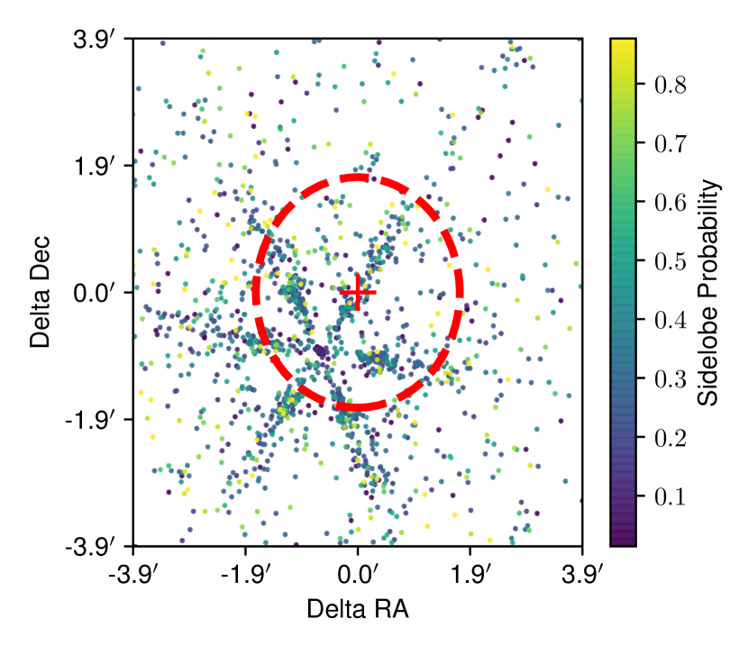
Figure 12: The accumulated radio components from the FIRST catalogue surrounding sources whose images shared a single BMU that exhibit PSF features in the radio channel. These components have been transformed following rotation and flipping information provided as outputs from PINK. The red circle denotes the $3.5\mathrm{\prime }$ angular size of the prototype weights with the red cross being position of the centre. The colour of each marker corresponds to the sidelobe probability of each component included as part of the FIRST catalogue calculated by the ensemble of decision trees.

We are capable of performing a similar procedure using exclusively the data products from our trained SOM with no a priori knowledge about the sidelobe characteristics. For example, we located one neuron that exhibited remnants of the VLA PSF around a bright source offset from the centre. From mapping all images in our training dataset we identified 126 with this neuron as their BMU. We searched $6\mathrm{\prime }$ around the 126 positions these images are centred towards and found a total of $2,025$ radio components in our FSC. The 126 transformations derived by PINK were applied to the corresponding set of returned components. We show these transformed component offsets in Figure 12, where the VLA PSF can be seen as an over-densities of radio components. For illustration we also show how these features can be extended beyond the $$$\times$$$ field of view of the prototype weights.

Arguably the sidelobe probabilities from Helfand et al. (2015) may be lower than what could qualitatively be expected judging by the density of components from Figure 12. To illustrate we first shifted the origin of Figure 12 to the approximate centre of the VLA PSF feature and converted the delta-offset Cartesian positions to a polar coordinate system. We mask both the inner most $0.2\mathrm{\prime }$ region to remove legitimate, bright FIRST components and the region beyond $2\mathrm{\prime }$ to remain near the bounds of the field of view of the neuron. After applying this mask there were $1,008$ valid FIRST components. Examining the collection of angles from the polar projection in Figure 13 shows a highly non-uniform distribution with peaks spaced by $\pi\text{/}3\text{\,}\mathrm{rad}$, each corresponding to a spoke along the VLA PSF. We then computed the running median value of the corresponding sidelobe probabilities for 50 components at a time (after sorting them by their angle). Comparing the distribution of angles to the computed running median shows that, surprisingly, the components have lower sidelobe probability estimates when there is an excess of components. Likely, this is a manifestation of the poor invariance to affine transforms of the ensemble of decision tree classifiers. These results suggests that PINK would be an excellent tool towards identifying and characterising artefact components.

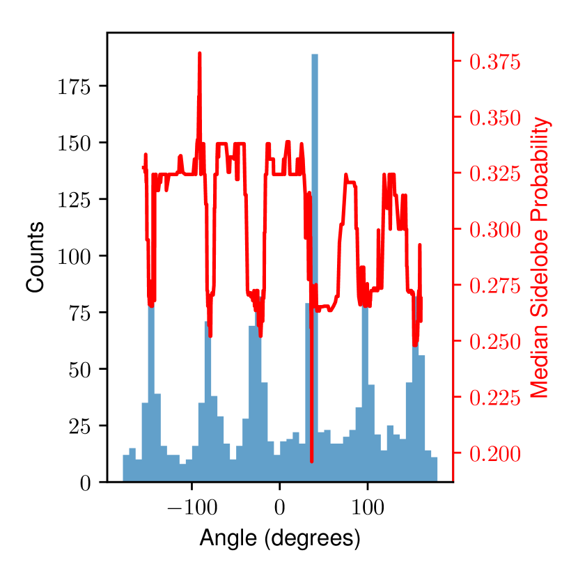
Figure 13: The distribution of $1,008$ angles from components after being transformed to a polar coordinate system. Each peak corresponds to a spoke of the VLA PSF. The largest count corresponds to a position towards the 126 position centred on a sidelobe artefact. Overlaid as a red line is the running median across 50 components (after sorting by their angle) of the sidelobe probability from the FIRST catalogue. For the running median we blank out edge effects from the trend.

For future catalogue releases (either of the FIRST catalogue we present in this work or other surveys) this can be combined with a probability treatment of the neurons (§7.2) to obtain a likelihood measure of a radio component being a genuine source component or simply an imaging artefact.

7.5 Extending the Annotation Labelling Scheme

We explicitly elected for a minimal annotation scheme to demonstrate the immediate potential of our overall collation framework. For this reason we restricted our annotations to describe positions of features in Cartesian space. No additional properties were recorded (e.g. core label, presence of sidelobes, optimal threshold level for individual neurons, Fanaroff-Riley type). Subsequent processing steps use these positions in combination with simple, generalised stages to extract knowledge about objects and their, potentially resolved, morphologies. In many ways this transfer of knowledge from the lower dimensional embedding (set of SOM neurons) could further be refined by also recording these higher order products during the annotation stage.

As an example, a user defined threshold value would be of particular importance. We used a simple method that would attempt to identify islands of contiguous pixels that encompassed the user specified pixel positions (Figure 3). This method sometimes failed for neurons with weak or absent features, which was particularly common for the infrared channel of neurons which learnt to identify radio sidelobe artefacts present around bright FIRST source components. As a consequence there are cases of artificial groups with ill-defined infrared host positions. A more sophisticated annotation scheme would be able to largely avoid this by carrying forward strict labels or flagging operations with a more reasonable thresholding level defined explicitly during the annotation stage. If necessary user-defined regions could also be interactively defined and used in place of a simple pixel-threshold value.

Developing this idea further, regions within the prototype weights could be defined to carry further information or actions. For instance, the filters we characterise in Figure 3 will only be used to group together components and sources. Expanding these to include regions that will ensure components remain disassociated under all conditions may help to ensure our greedy collation process considers all available information when crafting component groups.

8 Conclusions

We have demonstrated a new approach towards identifying related radio components and isolating their corresponding infrared host galaxies using PINK, an unsupervised machine learning algorithm. Unlike supervised methods, which can be likened to attempting to model the operation of a generalised function, an unsupervised machine learning algorithm attempts to model the structure of an assumed dataset. PINK implements a similarity measure that is rotationally and flipping invariant by searching for a transform that best aligns an image with structures that are either predefined or learnt through an iterative training process. In this study we have used PINK to

1. applied an unsupervised machine learning method against a training set of radio and infrared images to produce a set of physically meaningful prototype morphologies without the need of training labels, and

2. constructed a framework to meaningfully explore the previously unstructured complex image data, including the introduction of a statistic to identify bent radio morphologies.

Using the PINK products and outputs from our collation process we have

1. used data products from PINK to collate together related FIRST radio components and predict their corresponding infrared host,

2. demonstrated an ability to efficiently extract rare and unusual object morphologies, and

3. compiled a list of 17 GRG that were identified after isolating their resolved lobes with our collation method.

Throughout we maintained a simplified workflow to demonstrate a new methodology towards this difficult problem. In the future we will further develop our framework to better exploit the data products produced by PINK with with emphasis on SKA surveys.

Data Availability

Image and catalogue data that were used throughout this study are publicly accessible from their respective survey data portals. Output source catalogues will be made publicly available alongside this article and through data access portals (e.g. ViZieR). The corresponding authors may also be contacted for further details if required.

Appendix A Layer Two SOM

In Figure 14 we present the Layer Two SOM constructed in §4.3. We have divided it into 25 $8\times 8$ regions to allow the PINK prototype weights to be visualised. The coordinate labels are consistent among each of the 25 regions.

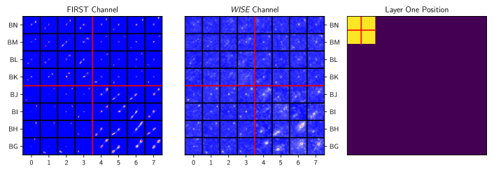
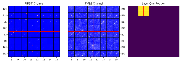
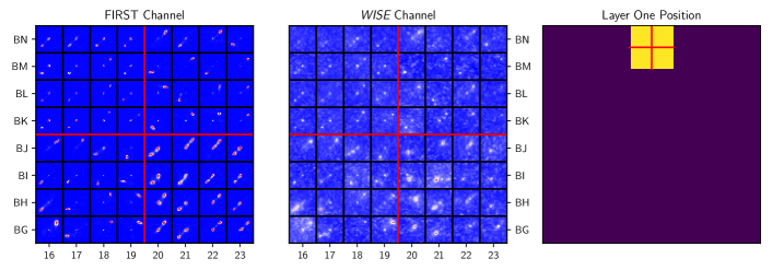
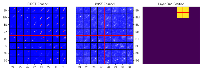
Figure 14: The FIRST (left) and WISE (middle) channels of the Layer Two SOM constructed by concatenating 100 $4\times$ SOMs. The black vertical and horizontal lines represent the boundary between individual neurons on the lattice, while the red vertical and horizontal lines represent boundaries between individual $4\times 4$ SOMs. Each of the SOMs were trained using the same data preprocessing and training stages as Layer One. The Layer One position (right) shows the relative position of the four SOMs on the Layer One SOM (Figure 2).

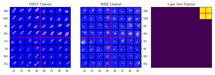
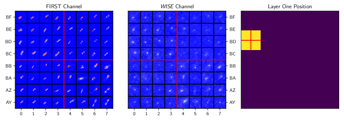
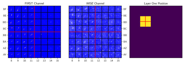
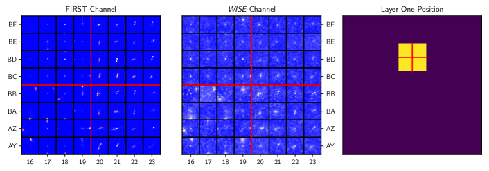
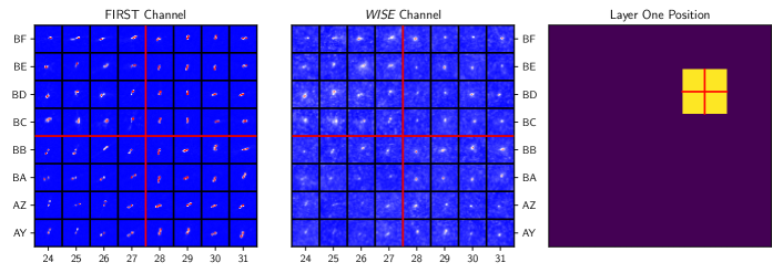
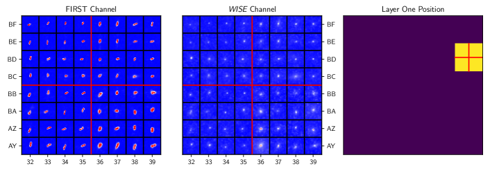
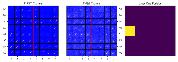
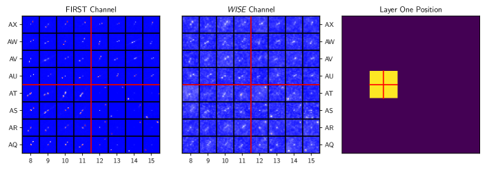
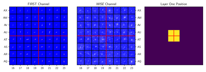
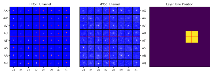
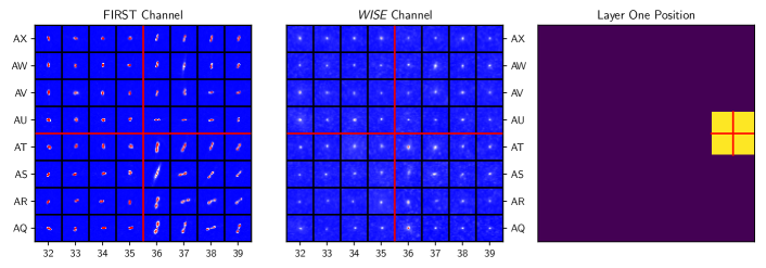
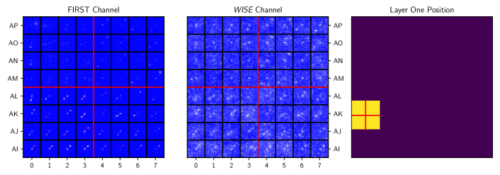
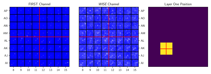
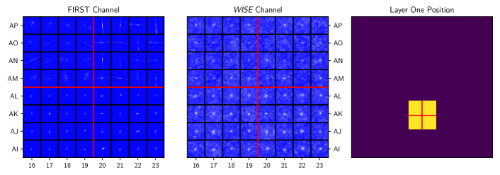
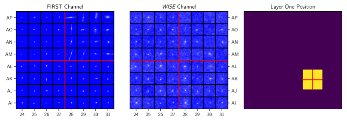
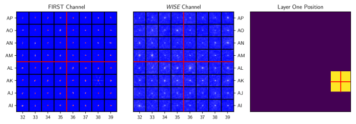
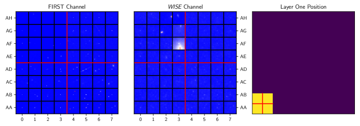
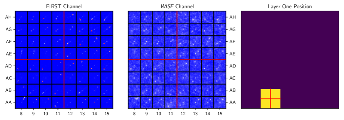
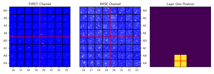
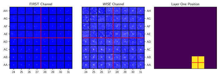
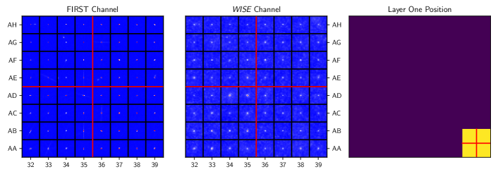
Figure 14: (Cont.) The FIRST (left) and WISE (middle) channels of the Layer Two SOM constructed by concatenating 100 $4\times$ SOMs. The black vertical and horizontal lines represent the boundary between individual neurons on the lattice, while the red vertical and horizontal lines represent boundaries between individual $4\times 4$ SOMs. Each of the SOMs were trained using the same data preprocessing and training stages as Layer One. The Layer One position (right) shows the relative position of the four SOMs on the Layer One SOM (Figure 2).

Figure 14: (Cont.) The FIRST (left) and WISE (middle) channels of the Layer Two SOM constructed by concatenating 100 $4\times$ SOMs. The black vertical and horizontal lines represent the boundary between individual neurons on the lattice, while the red vertical and horizontal lines represent boundaries between individual $4\times 4$ SOMs. Each of the SOMs were trained using the same data preprocessing and training stages as Layer One. The Layer One position (right) shows the relative position of the four SOMs on the Layer One SOM (Figure 2).

Figure 14: (Cont.) The FIRST (left) and WISE (middle) channels of the Layer Two SOM constructed by concatenating 100 $4\times$ SOMs. The black vertical and horizontal lines represent the boundary between individual neurons on the lattice, while the red vertical and horizontal lines represent boundaries between individual $4\times 4$ SOMs. Each of the SOMs were trained using the same data preprocessing and training stages as Layer One. The Layer One position (right) shows the relative position of the four SOMs on the Layer One SOM (Figure 2).

Figure 14: (Cont.) The FIRST (left) and WISE (middle) channels of the Layer Two SOM constructed by concatenating 100 $4\times$ SOMs. The black vertical and horizontal lines represent the boundary between individual neurons on the lattice, while the red vertical and horizontal lines represent boundaries between individual $4\times 4$ SOMs. Each of the SOMs were trained using the same data preprocessing and training stages as Layer One. The Layer One position (right) shows the relative position of the four SOMs on the Layer One SOM (Figure 2).

Figure 14: (Cont.) The FIRST (left) and WISE (middle) channels of the Layer Two SOM constructed by concatenating 100 $4\times$ SOMs. The black vertical and horizontal lines represent the boundary between individual neurons on the lattice, while the red vertical and horizontal lines represent boundaries between individual $4\times 4$ SOMs. Each of the SOMs were trained using the same data preprocessing and training stages as Layer One. The Layer One position (right) shows the relative position of the four SOMs on the Layer One SOM (Figure 2).

Figure 14: (Cont.) The FIRST (left) and WISE (middle) channels of the Layer Two SOM constructed by concatenating 100 $4\times$ SOMs. The black vertical and horizontal lines represent the boundary between individual neurons on the lattice, while the red vertical and horizontal lines represent boundaries between individual $4\times 4$ SOMs. Each of the SOMs were trained using the same data preprocessing and training stages as Layer One. The Layer One position (right) shows the relative position of the four SOMs on the Layer One SOM (Figure 2).

Appendix B Example Tables

We include five row extracts of our FSC and GRC catalogues.

GID	idx	neuron_index	ED	flip	rotation
279496	0	(29, 14, 0)	27.301	1	0.297
215840	1	(17, 8, 0)	23.787	1	1.239
717469	2	(35, 36, 0)	19.560	0	0.279
215841	3	(17, 8, 0)	22.714	1	4.381
474119	4	(36, 29, 0)	12.071	1	2.356

Table 5: Five example rows of our compiled FSC catalogue. Columns correspond to those described by Table 3. Each row also carries with it the original information from FIRST described in (Helfand et al., 2015). A value of ‘1’ in the ‘flip‘ column corresponds to an image being flipped as part of its transform.

GID	prob_host	comp_host	grp_flag	D_idx	D	SP_idx	SP	Q	rel_g	rel_Q	rel_D	ir_pp_ra	ir_pp_dec
					′′		′′	′′				∘	∘
0	J085632.98+595746.9	(J085632.98+595746.9)	1	(28052, 28186)	149.21	(28065, 28137, 28197, 28213, 28203)	166.33	1.11	0.95	0.81	0.85	134.14	59.96
1	J085039.97+543753.4	(J085039.97+543753.4)	1	(68434, 68412)	114.90	(68458, 68418, 68446, 68408)	129.04	1.12	0.53	0.75	0.83	132.67	54.63
2	J151347.88+530834.1	(J151347.88+530834.1)	1	(81092, 81370)	139.94	(81118, 81130, 81211, 81335, 81350)	141.15	1.01	0.92	0.93	0.86	228.45	53.14
3	J140717.50+513213.4	(J140717.50+513213.4)	1	(95447, 95258)	151.76	(95461, 95421, 95450, 95371, 95337, 95286)	171.89	1.13	0.91	0.84	0.85	211.82	51.54
4	J125142.02+503424.8	(J125142.02+503424.8)	1	(103762, 103670)	131.31	(103758, 103703, 103688)	139.48	1.06	0.90	0.89	0.83	192.92	50.57

Table 6: Five example rows of our compiled GRC catalogue. Columns correspond to those described in Table 3.

References

- Abolfathi et al. (2018) Abolfathi B., et al., 2018, ApJS, 235, 42
- Aguado et al. (2019) Aguado D. S., et al., 2019, ApJS, 240, 23
- Alam et al. (2015) Alam S., et al., 2015, ApJS, 219, 12
- Albareti et al. (2017) Albareti F. D., et al., 2017, ApJS, 233, 25
- Alger et al. (2018) Alger M. J., et al., 2018, MNRAS, 478, 5547
- Astropy Collaboration et al. (2013) Astropy Collaboration et al., 2013, A&A, 558, A33
- Banfield et al. (2015) Banfield J. K., et al., 2015, MNRAS, 453, 2326
- Becker et al. (1995) Becker R. H., White R. L., Helfand D. J., 1995, ApJ, 450, 559
- Begelman et al. (1984) Begelman M. C., Blandford R. D., Rees M. J., 1984, Reviews of Modern Physics, 56, 255
- Blanton et al. (2004) Blanton E. L., Gregg M. D., Helfand D. J., Becker R. H., White R. L., 2004, in Mulchaey J. S., Dressler A., Oemler A., eds, Clusters of Galaxies: Probes of Cosmological Structure and Galaxy Evolution. p. 4 (arXiv:astro-ph/0303554)
- Brett et al. (2004) Brett D. R., West R. G., Wheatley P. J., 2004, MNRAS, 353, 369
- Capetti et al. (2002) Capetti A., Zamfir S., Rossi P., Bodo G., Zanni C., Massaglia S., 2002, A&A, 394, 39
- Cheung (2007) Cheung C. C., 2007, AJ, 133, 2097
- Cheung et al. (2009) Cheung C. C., Healey S. E., Landt H., Verdoes Kleijn G., Jordán A., 2009, ApJS, 181, 548
- Ching et al. (2017) Ching J. H. Y., et al., 2017, MNRAS, 464, 1306
- Crawford et al. (2017) Crawford E., Norris R. P., Polsterer K., 2017, in Lorente N. P. F., Shortridge K., Wayth R., eds, Astronomical Society of the Pacific Conference Series Vol. 512, Astronomical Data Analysis Software and Systems XXV. p. 109 (arXiv:1611.02829)
- Cutri (2013) Cutri R. M., 2013, VizieR Online Data Catalog, p. II/328
- Dabhade et al. (2017) Dabhade P., Gaikwad M., Bagchi J., Pand ey-Pommier M., Sankhyayan S., Raychaudhury S., 2017, MNRAS, 469, 2886
- Dabhade et al. (2019) Dabhade P., et al., 2019, arXiv e-prints, p. arXiv:1904.00409
- Day (1969) Day N. E., 1969, Biometrika, 56, 463
- Dennett-Thorpe et al. (2002) Dennett-Thorpe J., Scheuer P. A. G., Laing R. A., Bridle A. H., Pooley G. G., Reich W., 2002, MNRAS, 330, 609
- Downes et al. (1986) Downes A. J. B., Peacock J. A., Savage A., Carrie D. R., 1986, MNRAS, 218, 31
- Fanaroff & Riley (1974) Fanaroff B. L., Riley J. M., 1974, MNRAS, 167, 31P
- Galvin et al. (2019) Galvin T. J., et al., 2019, PASP, 131, 108009
- Geach (2012) Geach J. E., 2012, MNRAS, 419, 2633
- Ghahramani (2004) Ghahramani Z., 2004, Unsupervised Learning. Springer Berlin Heidelberg, Berlin, Heidelberg, pp 72–112, doi:10.1007/978-3-540-28650-9_5, https://doi.org/10.1007/978-3-540-28650-9_5
- Greisen & Calabretta (2002) Greisen E. W., Calabretta M. R., 2002, Astronomy & Astrophysics, 395, 1061
- Hagberg et al. (2008) Hagberg A. A., Schult D. A., Swart P. J., 2008, in Varoquaux G., Vaught T., Millman J., eds, Proceedings of the 7th Python in Science Conference. Pasadena, CA USA, pp 11 – 15
- Hancock et al. (2018) Hancock P. J., Trott C. M., Hurley-Walker N., 2018, Publ. Astron. Soc. Australia, 35, e011
- Helfand et al. (2015) Helfand D. J., White R. L., Becker R. H., 2015, ApJ, 801, 26
- Hinshaw et al. (2013) Hinshaw G., et al., 2013, ApJS, 208, 19
- Högbom (1974) Högbom J. A., 1974, A&AS, 15, 417
- Hogg (1999) Hogg D. W., 1999, arXiv e-prints, pp astro–ph/9905116
- Hunter (2007) Hunter J. D., 2007, Computing In Science & Engineering, 9, 90
- Jamrozy et al. (2008) Jamrozy M., Konar C., Machalski J., Saikia D. J., 2008, MNRAS, 385, 1286
- Johnston et al. (2008) Johnston S., et al., 2008, Experimental Astronomy, 22, 151
- Jonas & MeerKAT Team (2016) Jonas J., MeerKAT Team 2016, in MeerKAT Science: On the Pathway to the SKA. p. 1
- Kaiser et al. (1997) Kaiser C. R., Dennett-Thorpe J., Alexander P., 1997, MNRAS, 292, 723
- Kapińska et al. (2017) Kapińska A. D., et al., 2017, AJ, 154, 253
- Kohonen (1982) Kohonen T., 1982, Biological Cybernetics, 43, 59
- Leahy & Williams (1984) Leahy J. P., Williams A. G., 1984, MNRAS, 210, 929
- Lintott et al. (2008) Lintott C. J., et al., 2008, MNRAS, 389, 1179
- Lloyd (1982) Lloyd S. P., 1982, IEEE Transactions on Information Theory, 28, 129
- Lukic et al. (2018) Lukic V., Brüggen M., Banfield J. K., Wong O. I., Rudnick L., Norris R. P., Simmons B., 2018, MNRAS, 476, 246
- Lynden-Bell (1969) Lynden-Bell D., 1969, Nature, 223, 690
- Malarecki et al. (2015) Malarecki J. M., Jones D. H., Saripalli L., Staveley-Smith L., Subrahmanyan R., 2015, MNRAS, 449, 955
- Mao et al. (2010) Mao M. Y., Sharp R., Saikia D. J., Norris R. P., Johnston-Hollitt M., Middelberg E., Lovell J. E. J., 2010, MNRAS, 406, 2578
- Mohan & Rafferty (2015) Mohan N., Rafferty D., 2015, PyBDSF: Python Blob Detection and Source Finder (ascl:1502.007)
- Norris (2017a) Norris R. P., 2017a, Nature Astronomy, 1, 671
- Norris (2017b) Norris R. P., 2017b, Publ. Astron. Soc. Australia, 34, e007
- Norris et al. (2011) Norris R. P., et al., 2011, Publ. Astron. Soc. Australia, 28, 215
- O’Brien et al. (2018) O’Brien A. N., Norris R. P., Tothill N. F. H., Filipović M. D., 2018, MNRAS, 481, 5247
- Pâris et al. (2017) Pâris I., et al., 2017, A&A, 597, A79
- Pearson (1901) Pearson K., 1901, The London, Edinburgh, and Dublin Philosophical Magazine and Journal of Science, 2, 559
- Pedregosa et al. (2011) Pedregosa F., et al., 2011, Journal of Machine Learning Research, 12, 2825
- Perley et al. (2011) Perley R. A., Chandler C. J., Butler B. J., Wrobel J. M., 2011, ApJ, 739, L1
- Polsterer et al. (2016) Polsterer K. L., Gieseke F., Igel C., Doser B., Gianniotis N., 2016, in European Symposium on Artificial Neural Networks.
- Proctor (2016) Proctor D. D., 2016, ApJS, 224, 18
- Ralph et al. (2019) Ralph N. O., et al., 2019, PASP, 131, 108011
- Robotham et al. (2018) Robotham A. S. G., Davies L. J. M., Driver S. P., Koushan S., Taranu D. S., Casura S., Liske J., 2018, MNRAS, 476, 3137
- Safouris et al. (2009) Safouris V., Subrahmanyan R., Bicknell G. V., Saripalli L., 2009, MNRAS, 393, 2
- Saripalli & Roberts (2018) Saripalli L., Roberts D. H., 2018, ApJ, 852, 48
- Saripalli & Subrahmanyan (2009) Saripalli L., Subrahmanyan R., 2009, ApJ, 695, 156
- Shimwell et al. (2019) Shimwell T. W., et al., 2019, A&A, 622, A1
- Subrahmanyan et al. (2008) Subrahmanyan R., Saripalli L., Safouris V., Hunstead R. W., 2008, ApJ, 677, 63
- Tang et al. (2019) Tang H., Scaife A. M. M., Leahy J. P., 2019, MNRAS, 488, 3358
- Tasdemir & Merényi (2009) Tasdemir K., Merényi E., 2009, Neural Networks, IEEE Transactions on, 20, 549
- Tingay et al. (2013) Tingay S. J., et al., 2013, Publ. Astron. Soc. Australia, 30, e007
- Torniainen et al. (2008) Torniainen I., et al., 2008, A&A, 482, 483
- Van Der Walt et al. (2011) Van Der Walt S., Colbert S. C., Varoquaux G., 2011, Computing in Science & Engineering, 13, 22
- Way et al. (2011) Way M. J., Gazis P. R., Scargle J. D., 2011, ApJ, 727, 48
- Wayth et al. (2018) Wayth R. B., et al., 2018, Publ. Astron. Soc. Australia, 35, 33
- Wright et al. (2010) Wright E. L., et al., 2010, AJ, 140, 1868
- Wu et al. (2019) Wu C., et al., 2019, MNRAS, 482, 1211
- Yang et al. (2019) Yang X., et al., 2019, arXiv e-prints, p. arXiv:1905.06356
- jon (2001) 2001, SciPy: Open source scientific tools for Python, http://www.scipy.org/
- van Haarlem et al. (2013) van Haarlem M. P., et al., 2013, A&A, 556, A2
- van der Walt et al. (2014) van der Walt S., et al., 2014, The Journal of Life and Environmental Sciences, 2, e453