Domain Contrast for Domain Adaptive Object Detection

Abstract

We present Domain Contrast (DC), a simple yet effective approach inspired by contrastive learning for training domain adaptive detectors. DC is deduced from the error bound minimization perspective of a transferred model, and is implemented with cross-domain contrast loss which is plug-and-play. By minimizing cross-domain contrast loss, DC guarantees the transferability of detectors while naturally alleviating the class imbalance issue in the target domain. DC can be applied at either image level or region level, consistently improving detectors’ transferability and discriminability. Extensive experiments on commonly used benchmarks show that DC improves the baseline and state-of-the-art by significant margins, while demonstrating great potential for large domain divergence.

1 Introduction

Modern object detectors [25, 21] have achieved unprecedented progress with the rise of convolutional neural networks (CNNs). Although, their practical application to real-world scenarios remains limited for the following two reasons: 1) Supervised learning of detectors for different scenarios requires repeated human effort on data annotation, and 2) offline-trained detectors typically degrade with changes in the scene or camera. Domain adaptive detection, which transfers detectors trained within a label-rich domain ($i.e.$, annotated datasets) to an unlabeled domain ($i.e.$, real-world scenarios), have attracted increasing interests because of their potential to solve these problems [8, 28, 35, 30].

Domain adaptive detection is usually explored with unsupervised domain adaptation (UDA) methods. Such methods typically maximize the “transferability" of models by aligning the feature distributions of domains [8] or taking advantages of adversarial and generative models [2, 15]. The underlying hypothesis is that accurate feature alignment across domains produces good transferability.

Recent studies [6] have shown that transferability and discriminability are in fact two sides of a same coin. The transferring process, $e.g.,$ minimizing Maximum Mean Discrepancy (MMD) [13], could deteriorate the discriminability of models and features [32]. This would be more severe in the object detection problem, considering the large imbalance of negative and positive instances which need to be classified. Slight degradation of model discriminability could therefore cause a significant increase of false positives in the target domain.

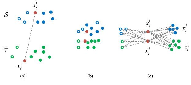
Figure 1: Illustration of Domain Contrast. (a) The reduction of domain divergence (distance between $x_{s}^{i}$ and $x_{t}^{i}$) towards aligning feature distributions of the source domain $\mathcal{S}$ and the target domain $\mathcal{T}$. (b) The reduction of the domain divergence could reduce the discriminability of models, $i.e.$, samples from different categories are mixed together. (c) Domain contrast simultaneously reduces domain divergence by minimizing the cross-domain distance while preserving model discriminability by maximizing the distances between samples from different categories.

In this paper, we derive the Domain Contrast (DC) method from the perspective of error bound minimization when transferring detectors from a source to a target domain. Minimizing error bound is converted to optimize DC loss, which defines the cross-domain similarity and inter-class distance for each min-batch of samples, Fig. 1. DC guarantees the transferability of detectors by maximizing the $cosine$ similarity between each sample with its cross-domain counterparts. This also preserves the discriminability of transferred detectors by minimizing the similarity between samples from different categories in a mini-batch.

To define DC, training sample images are translated from the source/target to the target/source domain via a CycleGAN method [34]. With translated images, a detector is trained using annotated samples in the source domain and fine-tuned using DC loss from the source to the target domain. In turn, the detector is fine-tuned using the DC loss from the target to the source domain. DC loss is applied at image- and region-level, consistently improving the transferability and discriminability of detectors.

The contributions of this work are summarized as follows:

• A simple-yet-effective domain contrast (DC) method for transfer learning, where the DC loss is derived from the perspective of error bound minimization. Minimization of DC loss drives feature alignment ($i.e.$, transferability) across domains while preserving model discriminability in the target domain.

• A domain adaptive detector considering the class imbalance issue. The detector leverages DC loss at image level and region level to handle the detector transfer problem, achieving state-of-the-art performance on benchmarks with large domain divergence.

2 Related Work

Unsupervised Domain Adaptation (UDA). UDA aims to minimize the classification error when transferring the model trained within a source domain to an unlabelled target domain. UDA has been extensively explored in a number of computer vision specializations, including image classification [20, 24, 3, 12, 22], image recognition [10, 33], and object detection [8, 28, 35, 18].

One line of UDA methods devoted to align feature distributions of source and target domains by minimizing the domain divergence [22, 12]. For example, Maximum Mean Discrepancy (MMD) [13] was proposed as a domain distance metric to minimize the domain divergence in the Reproducing Kernel Hilbert Space (RKHS) [22, 23]. Progressive domain distance minimization [5] was achieved by mining pseudo labels to fine-tune the model. The other line of methods [2, 15] attempted to reduce the domain divergence by taking advantages of adversarial and generative models which confuse domains while aligning feature distributions. The CyCADA method [15] transferred samples across domains at both pixel- and feature-levels. Domain confusion loss [12] was designed to learn domain-invariant features. The descrepancy-based method [26] aligned distributions of source and target domains by learning features to minimize classifiers’ output discrepancy.

Domain Adaptive Detection. Early studies largely followed domain adaptive classification to align the features of source and target domains. DA-Faster R-CNN [8] pioneered these works by minimizing the discrepancy among two domains by exploring both image- and instance-level domain classifier in an adversarial manner. Mean Teacher with object relations [4] was applied for object distribution alignment, while integrating object relations with the measure of consistency cost between teacher and student modules. The Diversify and Match (DM) approach [18] generated various distinctive shifted domains from the source domain and aligned the distribution of the labeled data and encouraged features to be indistinguishable among the domains. Strong-and-Weak [28] method pursue weak alignment of image-level features and strong alignment of region-level features.

Despite progress, the essential difference between domain adaptive detection with domain adaptive classification is unfortunately ignored. On the one hand, source and target domains have distinct scene layouts and object combinations. Therefore, aligning the entire distributions of source and target images is implausible. On the other hand, object detectors face the serious class imbalance issue. Preserving model discriminability during domain adaptive detection is more important than that in image classification [35].

To preserve the discriminability, the Selective Cross-Domain approach [35] attempted aligning discriminative regions, namely those that are directly related to detection. The Hierarchical Transferability Calibration Network harmonized transferability and discriminability for cross-domain detection [6]. Nevertheless, these approaches used complex adversarial training and/or sample interpolation which hinders deployment and therefore practicability.

3 The Proposed Approach

Let $\mathcal{S}$ and $\mathcal{T}$ respectively denote a source and a target domain. The corresponding samples of $\mathcal{S}$ and $\mathcal{T}$ are denoted as $\{x^{i}_{s}\}_{i=1}^{N}$ and $\{x^{i}_{t}\}_{i=1}^{N}$. $f_{\mathcal{S}}:\mathcal{X}\rightarrow\{0,1\}$ and $f_{\mathcal{T}}:\mathcal{X}\rightarrow\{0,1\}$ denote functions which map the input samples $\mathcal{X}$ to a binary label space. $f_{\mathcal{T}}(x_{s}^{i})=f_{\mathcal{T}}(x_{t}^{i})$ and $f_{\mathcal{S}}(x_{s}^{i})=f_{\mathcal{S}}(x_{t}^{i})$ mean that the sample labels are consistent regardless of the domains. Domain adaptation targets at transferring a model ($i.e.$, the detector) optimized for $f_{\mathcal{S}}$ to $\mathcal{T}$ towards optimizing $f_{\mathcal{T}}$.

3.1 Domain Contrast

Error Bound Minimization. The source and target domains share an identical label space, but violate the $i.i.d.$ assumption as they are sampled from different data distributions. Given a model hypothesis $h\in\mathcal{H}$, the expected error [1] within the target domain are bounded as

$$\begin{split}\mathcal{R}_{\mathcal{T}}(h,f_{\mathcal{T}})&\leq\mathcal{R}_{\mathcal{T}}(h,f_{\mathcal{S}})+|\mathcal{R}_{\mathcal{T}}(h,f_{\mathcal{T}})-\mathcal{R}_{\mathcal{T}}(h,f_{\mathcal{S}})|,\\ \end{split}$$ (1)

where $\mathcal{R}_{\mathcal{T}}(h,f_{\mathcal{T}})$ and $\mathcal{R}_{\mathcal{T}}(h,f_{\mathcal{S}})$ respectively denote the empirical error of hypothesis $h$ about labels in the target and source domains. To minimize the error bound defined by Eq. 1 is to minimize $|\mathcal{R}_{\mathcal{T}}(h,f_{\mathcal{T}})-\mathcal{R}_{\mathcal{T}}(h,f_{\mathcal{S}})|$ and $\mathcal{R}_{\mathcal{T}}(h,f_{\mathcal{T}})$, which aligns the two domains while preserving the discriminability of the trained model in the target domain.

In the context of CNN, with the binary cross entropy loss, we have

$$\begin{split}\mathcal{R}_{\mathcal{T}}(h,f_{\mathcal{S}})&=\frac{1}{N}\sum_{i}{\bigg{(}-f_{\mathcal{S}}(x_{t}^{i})\log(h(x_{t}^{i}))-(1-f_{\mathcal{S}}(x_{t}^{i}))\log(1-h(x_{t}^{i}))\bigg{)}},\end{split}$$ (2)

and

$$\begin{split}\mathcal{R}_{\mathcal{T}}(h,f_{\mathcal{T}})&=\frac{1}{N}\sum_{i}{\bigg{(}-f_{\mathcal{T}}(x_{t}^{i})\log(h(x_{t}^{i}))-(1-f_{\mathcal{T}}(x_{t}^{i}))\log(1-h(x_{t}^{i}))\bigg{)}},\end{split}$$ (3)

where $N$ denotes the number of samples. Subtracting Eq. 3 from Eq. 2, we have

$$\begin{split}|\mathcal{R}_{\mathcal{T}}(h,f_{\mathcal{T}})-\mathcal{R}_{\mathcal{T}}(h,f_{\mathcal{S}})|&=\bigg{|}\frac{1}{N}\sum_{i}{\bigg{(}-f^{\prime}(x_{t}^{i})\log(\frac{h(x_{t}^{i})}{1-h(x_{t}^{i})})\bigg{)}}\bigg{|},\\ \end{split}$$ (4)

where $f^{\prime}(x)=f_{\mathcal{T}}(x)-f_{\mathcal{S}}(x)$. For the optimal hypothesis $h^{*}$, it is assumed that the empirical error in the source domain is small enough, $i.e.$, $\mathcal{R}_{\mathcal{S}}(h^{*},f_{\mathcal{S}})\rightarrow 0$, and the discriminability of $h^{*}$ in $\mathcal{T}$ is smaller than that in $S$, as

$$\begin{split}|\log(\frac{h^{*}(x_{t}^{i})}{1-h^{*}(x_{t}^{i})})|&\leq|\log(\frac{h^{*}(x_{s}^{i})}{1-h^{*}(x_{s}^{i})})|.\end{split}$$ (5)

We therefore have

$$\begin{split}-f^{\prime}(x_{t}^{i})\log(\frac{h^{*}(x_{t}^{i})}{1-h^{*}(x_{t}^{i})})&\leq-f^{\prime}(x_{s}^{i})\log(\frac{h^{*}(x_{s}^{i})}{1-h^{*}(x_{s}^{i})}).\end{split}$$ (6)

Substituting Eq. 4 to Eq. 6, we have

$$\begin{split}|\mathcal{R}_{\mathcal{T}}(h^{*},f_{\mathcal{T}})-\mathcal{R}_{\mathcal{T}}(h^{*},f_{\mathcal{S}})|&\leq|\mathcal{R}_{\mathcal{S}}(h^{*},f_{\mathcal{T}})-\mathcal{R}_{\mathcal{S}}(h^{*},f_{\mathcal{S}})|.\end{split}$$ (7)

According to Eq. 1, the error bound of hypothesis $h^{*}$ in the target domain is concluded as

$$\begin{split}\mathcal{R}_{\mathcal{T}}(h^{*},f_{\mathcal{T}})&\leq\mathcal{R}_{\mathcal{T}}(h^{*},f_{\mathcal{S}})+|\mathcal{R}_{\mathcal{S}}(h^{*},f_{\mathcal{T}})-\mathcal{R}_{\mathcal{S}}(h^{*},f_{\mathcal{S}})|\\ &\leq\mathcal{R}_{\mathcal{T}}(h^{*},f_{\mathcal{S}})+\mathcal{R}_{\mathcal{S}}(h^{*},f_{\mathcal{T}}).\end{split}$$ (8)

Domain Contrast (DC) Loss. To quantify $\mathcal{R}_{\mathcal{S}}(h^{*},f_{\mathcal{T}})$, $h^{*}$ is supposed to be a nearest neighbor classifier. The probability that a source domain sample $x_{s}^{i}$ has the same class label with it’s neighbors in the target domains is calculated as their similarity $\text{sim}(x_{s}^{i},x_{t}^{i})$, where $\text{sim}(u,v)=u^{\top}v/||u||||v||$ defines the $cosine$ similarity between two samples. Combining the probabilities to a softmax function, the nearest neighbor classifier $h^{*}$ is defined as

$$h^{*}(x_{t}^{i})=\frac{\sum_{j}f_{\mathcal{S}}(x_{s}^{j})\exp(\text{sim}(x_{t}^{i},x_{s}^{j}))}{\sum_{j}{\exp(\text{sim}(x_{t}^{i},x_{s}^{j}))}},$$ (9)

where $x_{t}^{i}$ is the $i^{th}$ sample transferred from the source to the target domain. Accordingly, minimization of the empirical error of a source model in the target domain, $\mathcal{R}_{\mathcal{T}}(h^{*},f_{\mathcal{S}})$, can be implemented by minimizing

$$\begin{split}\mathcal{R}_{\mathcal{T}}(h^{*},f_{\mathcal{S}})&=\frac{1}{N}\sum_{i}{-\log\bigg{(}\frac{\sum_{j}I(x_{t}^{i},x_{s}^{j})\exp(\text{sim}(x_{t}^{i},x_{s}^{j}))}{\sum_{j}{\exp(\text{sim}(x_{t}^{i},x_{s}^{j}))}}\bigg{)}}\\ &\leq\frac{1}{N}\sum_{i}{-\log\bigg{(}\frac{\exp(\text{sim}(x_{t}^{i},x_{s}^{i}))}{\sum_{j}{\exp(\text{sim}(x_{t}^{i},x_{s}^{j}))})}\bigg{)}},\end{split}$$ (10)

where $I(x_{1},x_{2})=1-|f_{\mathcal{S}}(x_{1})-f_{\mathcal{S}}(x_{2})|$. $N$ denotes the number of samples. Correspondingly, we approximately quantify the $\mathcal{R}_{\mathcal{S}}(h^{*},f_{\mathcal{T}})$ as

$$\begin{split}\mathcal{R}_{\mathcal{S}}(h^{*},f_{\mathcal{T}})&\leq\frac{1}{N}\sum_{i}{-\log\bigg{(}\frac{\exp(\text{sim}(x_{s}^{i},x_{t}^{i}))}{\sum_{j}{\exp(\text{sim}(x_{s}^{i},x_{t}^{j}))})}\bigg{)}}.\end{split}$$ (11)

According Eqs. 7, 10 and 11, minimizing the error bound defined by Eq. 1 can be fulfilled by optimizing network parameter $\theta$ to minimize

$$\begin{split}\mathcal{L}_{C}(\mathcal{S},\mathcal{T})=-\frac{1}{N}\sum_{i}{\log\bigg{(}\frac{\exp(\text{sim}(x_{t}^{i},x_{s}^{i}))}{\sum_{j}{\exp(\text{sim}(x_{t}^{i},x_{s}^{j}))})}\bigg{)}}-\frac{1}{N}\sum_{i}{\log\bigg{(}\frac{\exp(\text{sim}(x_{s}^{i},x_{t}^{i}))}{\sum_{j}{\exp(\text{sim}(x_{s}^{i},x_{t}^{j}))})}\bigg{)}},\end{split}$$ (12)

which is referred to as the DC loss.

Advantages of DC Loss. The DC loss is derived from the perspective of error bound minimization, while reflecting the similarity and dis-similarity (contrast) between samples across the domains. Minimizing DC loss drives learning feature representations that capture information shared between source and target domains but that are discriminative $i.e.$, different samples/instances in the two domains have small similarities ($i.e.$, large $cosine$ distances), Fig. 1.

It is known that during object detection the positive-negative class imbalance is an important issue. Such an issue has been widely explored in supervised detection, but unfortunately ignored by the domain adaptive detection, which could deteriorate the discriminability of transferred detectors. The nominator and denominator of the DC loss naturally incorporate sampling imbalance, which, during transfer, facilities alleviating class imbalance in the target domain. This is an advantage of DC loss compared to the Triplet Loss [19].

3.2 Domain Adaptive Detection

To implement domain adaptive detection, a base detector based on the deep network is first trained using the annotated data $\{x^{n}_{s},y^{n}_{s}\}_{n=1}^{N^{s}}$ in the source domain by minimizing the detection loss $\mathcal{L}_{D}(\theta)$. The trained base detector is then transferred to the target domain by fine-tuning the network and minimizing the image- and region-level DC loss $\mathcal{L}^{I}_{C,\mathcal{S}}(\theta)$ and $\mathcal{L}^{R}_{C,\mathcal{S}}(\theta)$. In turn, the detector is transferred to the source domain by minimizing the image-level DC loss $\mathcal{L}^{I}_{C,\mathcal{T}}(\theta)$ and fine-tuning the detector using $\mathcal{L}_{\mathcal{T}}^{R}(\theta)$, which is the pseudo ground-truth loss.

Base Detector. The Faster R-CNN [25] is employed as the base detector, which consists of three stages: convolutional feature extraction, region proposal generation (RPN) and bounding box prediction, Fig. 2. Each input image is represented as image-level features and RPN generates object region proposals, of which region-level features are extracted by ROI-pooling. With region-level features, the category labels and bounding boxes are predicted by classification and regression subnets. Detection loss $\mathcal{L}_{D}(\theta)$ is composed of the loss of the RPN and the loss of the subnets.

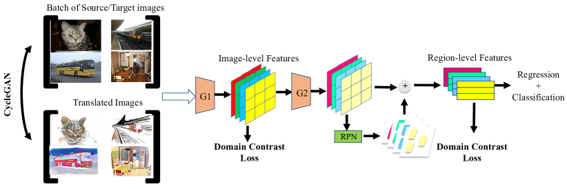
Figure 2: Illustration of the domain adaptive objector based upon CycleGAN and the proposed DC loss. CycleGAN is adopted to translate an image from the $\mathcal{S}/\mathcal{T}$ to the $\mathcal{T}/\mathcal{S}$ domain. $G1$ and $G2$ refer to convolutional layers. The detection network is first trained within $\mathcal{S}$ by minimizing the training loss $\mathcal{L}_{D}(\theta)$. The network then is transferred across domains by progressively minimizing the DC loss including $\mathcal{L}_{C,\mathcal{S}}^{I}(\theta)$, $\mathcal{L}_{C,\mathcal{S}}^{R}(\theta)$, and $\mathcal{L}_{C,\mathcal{T}}^{I}(\theta)$ and the pseudo ground-truth loss $\mathcal{L}_{\mathcal{T}}^{R}(\theta)$.

$\mathcal{S}\rightarrow\mathcal{T}$ Transfer. To transfer the Faster RCNN detector parameterized by $\theta$, we first translate each sample image $x_{s}^{i}$ from $\mathcal{S}$ to $\mathcal{T}$ using the CycleGAN method [34], which learns to translate an image from a source domain to a target domain given unpaired/paired examples. After iterative adversarial generation, the translated source images have similar styles with other images in the target domain.

Denote the features of a translated sample as $x_{s\rightarrow t}^{i}(I;\theta)$. For a batch of samples in $\mathcal{S}$ and their translated counterparts in $\mathcal{T}$, we construct a positive sample pair $(x_{s}^{i}(I;\theta),x_{s\rightarrow t}^{i}(I;\theta))$ and $N-1$ negative sample pairs $(x_{s}^{j}(I;\theta),x_{s\rightarrow t}^{i}(I;\theta))$. Given positive negative sample pairs, $\mathcal{S}\rightarrow\mathcal{T}$ transfer is implemented by fine-tuning the network parameter to minimize DC loss. By introducing a temperature parameter $\tau$ to Eq. 12, the image-level $\mathcal{S}\rightarrow\mathcal{T}$ DC loss is defined as

$$\begin{split}\mathcal{L}_{C,\mathcal{S}}^{I}(\theta)=&-\frac{1}{N}\sum_{i}{\log\bigg{(}\frac{\exp(\text{sim}(x_{s\rightarrow t}^{i}(I;\theta),x_{s}^{i}(I;\theta))/\tau)}{\sum_{j}{\exp(\text{sim}(x_{s\rightarrow t}^{i}(I;\theta),x_{s}^{j}(I;\theta))/\tau)})}\bigg{)}}\\ &-\frac{1}{N}\sum_{i}{\log\bigg{(}\frac{\exp(\text{sim}(x_{s}^{i}(I;\theta),x_{s\rightarrow t}^{i}(I;\theta))/\tau)}{\sum_{j}{\exp(\text{sim}(x_{s}^{i}(I;\theta),x_{s\rightarrow t}^{j}(I;\theta))/\tau)})}\bigg{)}},\end{split}$$ (13)

where $x^{i}(I;\theta)$ denotes the features in the last convolutional layer for a sample image.

In each image, we randomly select at the most two ground-truth bounding boxes for transfer. The features of selected proposals in an image are concatenated to a long vector, denoted as $x^{i}(R;\theta)$. The region-level contrast loss $\mathcal{L}_{C,\mathcal{S}}^{R}(\theta)$ can be calculated by replacing the image-level features $x^{i}(I;\theta)$ with the region-level features $x^{i}(R;\theta)$.

$\mathcal{T}\rightarrow\mathcal{S}$ Transfer. In a similar way the image-level $\mathcal{T}\rightarrow\mathcal{S}$ DC loss is defined as

$$\begin{split}\mathcal{L}_{C,\mathcal{T}}^{I}(\theta)=&-\frac{1}{N}\sum_{i}{\log\bigg{(}\frac{\exp(\text{sim}(x_{t}^{i}(I;\theta),x_{t\rightarrow s}^{i}(I;\theta)/\tau)}{\sum_{j}{\exp(\text{sim}(x_{t}^{i}(I;\theta),x_{t\rightarrow s}^{j}(I;\theta)/\tau)})}\bigg{)}}\\ &-\frac{1}{N}\sum_{i}{\log\bigg{(}\frac{\exp(\text{sim}(x_{t\rightarrow s}^{i}(I;\theta),x_{t}^{i}(I;\theta)/\tau)}{\sum_{j}{\exp(\text{sim}(x_{t\rightarrow s}^{i}(I;\theta),x_{t}^{j}(I;\theta)/\tau)})}\bigg{)}},\end{split}$$ (14)

As there is no ground-truth object annotated in the target domain, the region-level transfer can not be directly applied. We thereby first translate all the training image from $\mathcal{T}$ to $\mathcal{S}$ using the CycleGAN method. We then use the detector trained in $\mathcal{S}$ to detect high-scored regions in the translated images as pseudo ground-truth objects. With the pseudo ground-truth objects, region-level $\mathcal{T}\rightarrow\mathcal{S}$ transfer is carried out by fine-turning the detector to minimize the detection loss $\mathcal{L}_{\mathcal{T}}^{R}(\theta)$ for pseudo ground-truth objects.

4 Experiment

We analyzed the proposed domain adaptation method by training a detector in the PASCAL VOC dataset and transferring [11] it to the Clipart dataset [16] for performance evaluation. We also transferred detectors across domains, Pascal VOC $\rightarrow$ Comic2K and PASCAL $\rightarrow$ WaterColor2K [16], where large domain divergence exists.

4.1 Experimental Setting

Faster R-CNN with the ResNet101 [14] backbone pre-trained on the ImageNet [9] was employed as the base detector. While training the domain adaptive detector, the inputs were a mini-batch of images pairs, including $N$ (batch size) annotated images from the source domain and $N$ unannotated images from the target domain. We set the shorter side of the image to 600 pixels following the setting in of Faster RCNN [25]. The detection network (detector) was trained with a learning rate of 0.001 in the first 5 epochs and decreased to 0.0001 in the following 2 epochs. The iteration number of each epoch is calculated by the sample number divided by the batch size. The mean Average Precision(mAP) for all object categories in the dataset was used as the evaluation metric.

The DC loss is plug-and-play, which means it operates simply by fine-tuning the detector trained in the source domain. For each DC loss, the detector was fine-tuned by 5 epochs with a learning rate determined by experiments (Fig. 4). In this way, there is no regularization factor required to balance the importance of each loss terms defined in Sec. 3.2, which simplifies the parameter settings.

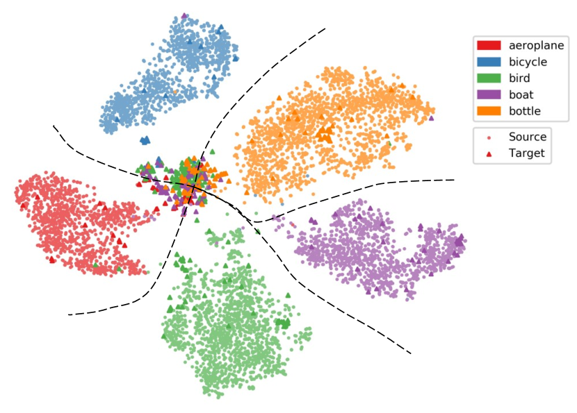
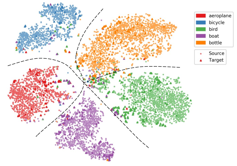
Figure 3: t-SNE of samples before (left) and after (right) domain adaptation. (Best viewed in color)

4.2 Model Effect

In Fig. 3, we compared the distributions of target samples before and after domain adaptation. Before adaptation, the target domain samples tends to be concentrated together and are difficult to discriminate. After domain adaptation using DC, the distribution of the target domain samples were well aligned with that of the source domain samples. At the same time, target samples can be well discriminated, which demonstrated the effect of the proposed DC method.

Table 1: Ablation study of detection performance (mAP%) and comparison with the state-of-the-arts when transferring a detector trained within PASCAL VOC to Clipart.

Method	aero	bike	bird	boat	bott.	bus	car	cat	chair	cow	table	dog	hrs	mbike	pers.	plant	sheep	sofa	train	tv	mAP
WST-BSR[17]	35.6	52.5	24.3	23.0	20.0	43.9	32.8	10.7	30.6	11.7	13.8	6.0	36.8	45.9	48.7	41.9	16.5	7.3	22.9	32.0	27.8
SWDA[27]	26.2	48.5	32.6	33.7	38.5	54.3	37.1	18.6	34.8	58.3	17.0	12.5	33.8	65.5	61.6	52.0	9.3	24.9	54.1	49.1	38.1
ICR-CCR [31]	28.7	55.3	31.8	26.0	40.1	63.6	36.6	9.4	38.7	49.3	17.6	14.1	33.3	74.3	61.3	46.3	22.3	24.3	49.1	44.3	38.3
HTCN[6]	33.6	58.9	34.0	23.4	45.6	57.0	39.8	12.0	39.7	51.3	21.1	20.1	39.1	72.8	63.0	43.1	19.3	30.1	50.2	51.8	40.3
DM[18]	25.8	63.2	24.5	42.4	47.9	43.1	37.5	9.1	47.0	46.7	26.8	24.9	48.1	78.7	63.0	45.0	21.3	36.1	52.3	53.4	41.8
Baseline	35.6	52.5	24.3	23.0	20.0	43.9	32.8	10.7	30.6	11.7	13.8	6.0	36.8	45.9	48.7	41.9	16.5	7.3	22.9	32.0	27.8
DC${}^{I}_{\mathcal{S\rightarrow T}}$	44.0	49.4	34.9	34.0	40.1	52.4	42.2	11.5	38.4	37.1	30.4	15.6	34.0	84.6	58.5	50.2	14.4	24.5	35.6	42.3	38.7
DC${}^{R}_{\mathcal{S\rightarrow T}}$	29.4	53.2	27.4	26.4	45.2	51.5	41.0	5.2	35.8	36.5	22.3	9.8	31.7	79.1	51.6	42.3	12.5	25.3	43.6	41.2	35.5
DC${}^{I,R}_{\mathcal{S\rightarrow T}}$	40.3	58.7	33.0	31.9	49.3	51.9	47.2	6.5	36.8	38.3	32.1	16.7	32.2	85.3	57.9	48.0	15.0	25.9	46.3	44.2	39.9
DC${}^{I}_{\mathcal{T\rightarrow S}}$	36.0	53.1	29.9	24.6	40.1	51.0	33.9	7.5	39.2	23.8	23.2	11.5	31.4	59.7	41.9	49.2	10.9	30.4	47.9	41.1	34.3
DC${}^{I,R}_{\mathcal{S\rightarrow T}}$-DC${}^{I}_{\mathcal{T\rightarrow S}}$	45.2	55.9	33.8	32.8	49.2	52.2	48.2	9.4	37.6	38.7	31.8	16.6	34.9	87.3	60.3	50.2	15.8	27.4	45.5	47.9	41.0
DC${}^{I,R}_{\mathcal{S\rightarrow T}}$- DC${}^{I,R}_{\mathcal{T\rightarrow S}}$	47.1	53.2	38.8	37.0	46.6	45.8	52.6	14.5	39.1	48.4	31.7	23.7	34.9	87.0	67.8	54.0	22.8	23.8	44.9	51.0	43.2
Oracle	33.3	47.6	43.1	38.0	24.5	82.0	57.4	22.9	48.4	49.2	37.9	46.4	41.1	54.0	73.7	39.5	36.7	19.1	53.2	52.9	45.0

Ablation Study. In Table 1, the effect of domain contrast was validated by performing $\mathcal{S}\rightarrow\mathcal{T}$ and $\mathcal{T}\rightarrow\mathcal{S}$ transfer step-by-step. Using solely the image-level $\mathcal{S}\rightarrow\mathcal{T}$ transfer (DC${}^{I}_{\mathcal{S\rightarrow T}}$) the mAP is improved by 10.9% (38.7% vs. 27.8%) which validated the effectiveness of our approach at reducing cross-domain divergence while improving detector discriminability. The region-level $\mathcal{S}\rightarrow\mathcal{T}$ transfer (DC${}^{R}_{\mathcal{S\rightarrow T}}$) improved the mAP by 7.7%. Combining the image-level and region-level $\mathcal{S}\rightarrow\mathcal{T}$ transfer (DC${}^{I,R}_{\mathcal{S\rightarrow T}}$) improved the mAP by 12.1% (39.9% vs. 27.8%).

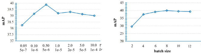
Figure 4: Ablation of parameter $\tau$, learning rate ($lr$), and batch size.

After performing image-level $\mathcal{T}\rightarrow\mathcal{S}$ transfer (DC${}^{I,R}_{\mathcal{S\rightarrow T}}$-DC${}^{I}_{\mathcal{T\rightarrow S}}$), the mAP is further improved by 1.1% (41.0% vs. 39.9%). Using the pseudo objects in the target domain to perform region-level $\mathcal{T}\rightarrow\mathcal{S}$ transfer was also effective, improving the mAP by 2.2% (43.2% vs. 41.0%). To reduce false positives, the threshold for pseudo object detection was set to be 0.95. Without whistle and bells, our method outperformed the state-of-the-art by 2.4% (43.2% vs. 41.8%), which was a significant margin considering the challenging task. We reported the “Oracle" result by training a Faster RCNN detector using the images within target domain but with the ground truth annotations, which is a reference for the performance upper-bound.

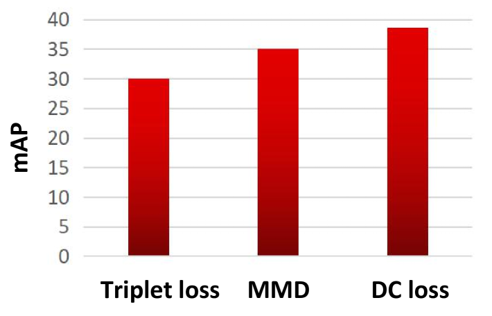
Figure 5: Comparison of mAPs of DC loss, Triplet Loss and MMD by performing image-level transfer from Pascal VOC to Clipart.

Parameter Setting. In Fig. 4, parameters $\tau$ and batch size were analyzed for DC loss. For each $\tau$, we determined the best learning rate by a linear search strategy. With a learning rate $5e$-6 and $\tau=0.5$ the best performance was achieved. The optimal $\tau$ selection improved 1.75% mAP, showing the importance of the temperature parameter. In contrast, the performance was not very sensitive to the batch size, $e.g.$, using a large batch size 8 slightly improved the mAP. This is different from unsupervised contrastive learning which often relies on large batch sizes [29, 7].

Imbalance Issue. In Fig. 5, we present the advantage of DC loss over the Triplet loss [19], which minimizes the intra-class distance of each positive sample pair and maximizes the inter-class distances of each positive-negative sample pair as $\sum_{j}\max(||x_{s}^{i}-x_{s\rightarrow t}^{i}||^{2}_{2}-||x_{s}^{i}-x_{s\rightarrow t}^{j}||^{2}_{2}+0.5,0)$. Triplet Loss reported much lower performance as it pursued maximizing the domain similarity and minimizing the similarity of a single pair of sample in a mini-batch but ignored the class imbalance issue in object detection. Such an imbalance issue was also ignored by the MMD method [32].

4.3 Performance and Comparison

Table 2: Performance comparison when transferring detectors from Pascal VOC to Comic2k.

Method	Base Detector	bike	bird	car	cat	dog	person	mAP
DT[16]	SSD+VGG16	43.6	13.6	30.2	16.0	26.9	48.3	29.8
WST-BSR[17]	SSD+VGG16	50.6	13.6	31.0	7.5	16.4	41.4	26.9
DM[18]	Faster RCNN+VGG16	-	-	-	-	-	-	34.5
Baseline	Faster RCNN+VGG16	38.5	10.5	14.7	15.1	15.2	29.8	20.6
	Faster RCNN+ResNet101	30.7	13.8	24.2	13.8	14.8	32.7	21.7
DC (ours)	Faster RCNN+VGG16	52.7	17.4	43.4	23.3	25.9	58.7	36.9
	Faster RCNN+ResNet101	51.9	23.9	36.7	27.1	31.5	61.0	38.7

Table 3: Performance comparison when transferring detectors from Pascal VOC to WaterColor2K.

Method	Base Detector	bike	bird	car	cat	dog	person	mAP
DT[16]	SSD+VGG16	82.8	47.0	40.2	34.6	35.3	62.5	50.4
WST-BSR[17]	SSD+VGG16	75.6	45.8	49.3	34.1	30.1	64.1	49.9
DM[18]	Faster RCNN+VGG16	-	-	-	-	-	-	52.0
SWDA[27]	Faster RCNN+ResNet101	82.3	55.9	46.5	32.7	35.5	66.7	53.3
Baseline	Faster RCNN+ResNet101	30.7	13.8	24.2	13.8	14.8	32.7	21.7
DC (ours)	Faster RCNN+ResNet101	76.7	53.2	45.3	41.6	35.5	70.0	53.7
Oracle	Faster RCNN+ResNet101	49.8	50.6	40.2	38.9	53.3	69.4	50.4

In Table 2, we evaluated the proposed method and compared it with state-of-the-art methods when transferring detectors from Pascal VOC to Comic2k [16]. The Comic2k dataset includes 2,000 comic images, 1,000 for training and the other 1,000 for test. It has 6 object classes which also exist in Pascal VOC. As the images in Comic2k are unrealistic images, Fig. 6, the domain divergence between the source (VOC) and the target domain (Comic2k) was predictably large. In this scenario, the proposed DC method outperformed the state-of-the-art method WST-BST [17] by 10.0% (36.9% vs. 26.9%) and DM [18] by 2.4% (36.9% vs. 34.5%). Using the ResNet-101 backbone further boosted the performance to 38.7%.

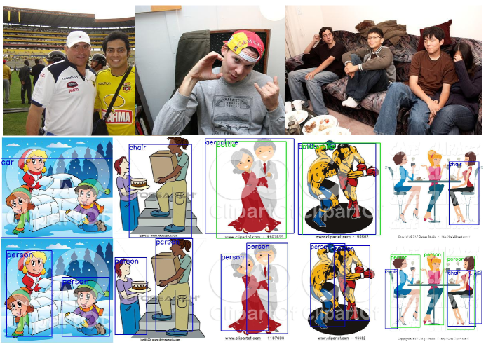
Figure 6: Detection examples from the Clipart dataset. Images from the source domain are in the first row. The results of the baseline method is in the second row and our detection results are in the last row. (Best viewed in color)

In Table 3, our method also outperformed the state-of-the-arts even the room for improvement was very small. The detection examples in Fig. 6 demonstrated the effectiveness of our method.

5 Conclusion

We presented Domain Contrast (DC), a simple yet effective approach to train domain adaptive detectors. This DC method is theoretically plausible because it was deduced from the perspective of error bound minimization about transfer learning. This DC method is conceptually simple and it can simultaneously guarantee the transferability of detectors while preserving the discriminability of transferred detectors by minimizing DC loss. DC significantly boosted the performance of domain adaptive detectors and improved the state-of-the-art on benchmark datasets of large domain divergence. This is the first time that the contrastive learning method has been applied to the domain adaptation problem and therefore provides a fresh insight to transfer learning.

Broader Impact

Benefit: The transfer learning community may benefit from this research. The proposed Domain Contrast method provides a fresh insight to transfer learning, which appears to have reached a plateau due to increasingly complex methodologies in recent years. With the code publicly available (please refer to the supplementary material), our research will also benefit the industry by improving the generalization capability of detectors trained within a label-rich domain ($i.e.$, publicly annotated datasets) to an unlabeled domain ($i.e.$, real-world scenarios).

Disadvantage: Our research may place researchers who continue using complex methodologies at a disadvantage. Our approach is simple, elegant, and effective, and could therefore be challenged by the status of quo of transfer learning.

Consequence: The failure of domain adaptation detection will not bring serious consequences, as the detectors trained in source domains can be the lower bound of the detection performance.

Data Biases: The proposed DC method DOES NOT leverage biases in the data. Whereas, the domain adaptive method aims to overcome data biases across domains.

References

- Ben-David et al. [2010] Shai Ben-David, John Blitzer, Koby Crammer, Alex Kulesza, Fernando Pereira, and Jennifer Wortman Vaughan. A theory of learning from different domains. Mach. Learn., 79(1-2):151–175, 2010.
- Bousmalis et al. [2017] Konstantinos Bousmalis, Nathan Silberman, David Dohan, Dumitru Erhan, and Dilip Krishnan. Unsupervised pixel-level domain adaptation with generative adversarial networks. In IEEE CVPR, pages 95–104, 2017.
- Busto and Gall [2017] Pau Panareda Busto and Juergen Gall. Open set domain adaptation. In IEEE ICCV, pages 754–763, 2017.
- Cai et al. [2019] Qi Cai, Yingwei Pan, Chong-Wah Ngo, Xinmei Tian, Lingyu Duan, and Ting Yao. Exploring object relation in mean teacher for cross-domain detection. In IEEE CVPR, pages 11457–11466, 2019.
- Chen et al. [2019] Chaoqi Chen, Weiping Xie, Wenbing Huang, Yu Rong, Xinghao Ding, Yue Huang, Tingyang Xu, and Junzhou Huang. Progressive feature alignment for unsupervised domain adaptation. In IEEE CVPR, pages 627–636, 2019.
- Chen et al. [2020a] Chaoqi Chen, Zebiao Zheng, Xinghao Ding, Yue Huang, and Qi Dou. Harmonizing transferability and discriminability for adapting object detectors. In IEEE CVPR, 2020a.
- Chen et al. [2020b] Ting Chen, Simon Kornblith, Mohammad Norouzi, and Geoffrey E. Hinton. A simple framework for contrastive learning of visual representations. CoRR, abs/2002.05709, 2020b.
- Chen et al. [2018] Yuhua Chen, Wen Li, Christos Sakaridis, Dengxin Dai, and Luc Van Gool. Domain adaptive faster R-CNN for object detection in the wild. In IEEE CVPR, pages 3339–3348, 2018.
- Deng et al. [2009] Jia Deng, Wei Dong, Richard Socher, Li-Jia Li, Kai Li, and Fei-Fei Li. Imagenet: A large-scale hierarchical image database. In IEEE CVPR, pages 248–255, 2009.
- Deng et al. [2018] Weijian Deng, Liang Zheng, Qixiang Ye, Guoliang Kang, Yi Yang, and Jianbin Jiao. Image-image domain adaptation with preserved self-similarity and domain-dissimilarity for person re-identification. In IEEE CVPR, pages 994–1003, 2018.
- Everingham et al. [2010] Mark Everingham, Luc Van Gool, Christopher K. I. Williams, John M. Winn, and Andrew Zisserman. The pascal visual object classes (VOC) challenge. Int. J. Comput. Vis., 88(2):303–338, 2010.
- Ganin and Lempitsky [2015] Yaroslav Ganin and Victor S. Lempitsky. Unsupervised domain adaptation by backpropagation. In ICML, volume 37, pages 1180–1189, 2015.
- Gretton et al. [2012] Arthur Gretton, Karsten M. Borgwardt, Malte J. Rasch, Bernhard Schölkopf, and Alexander J. Smola. A kernel two-sample test. J. Mach. Learn. Res., 13:723–773, 2012.
- He et al. [2016] Kaiming He, Xiangyu Zhang, Shaoqing Ren, and Jian Sun. Deep residual learning for image recognition. In IEEE CVPR, pages 770–778, 2016.
- Hoffman et al. [2018] Judy Hoffman, Eric Tzeng, Taesung Park, Jun-Yan Zhu, Phillip Isola, Kate Saenko, Alexei A. Efros, and Trevor Darrell. Cycada: Cycle-consistent adversarial domain adaptation. In ICML, pages 1994–2003, 2018.
- Inoue et al. [2018] Naoto Inoue, Ryosuke Furuta, Toshihiko Yamasaki, and Kiyoharu Aizawa. Cross-domain weakly-supervised object detection through progressive domain adaptation. In IEEE CVPR, pages 5001–5009, 2018.
- Kim et al. [2019a] Seunghyeon Kim, Jaehoon Choi, Taekyung Kim, and Changick Kim. Self-training and adversarial bakground regularization for unsupervised domain adaptive one-stage object detection. In IEEE ICCV, pages 6091–6100, 2019a.
- Kim et al. [2019b] Taekyung Kim, Minki Jeong, Seunghyeon Kim, Seokeon Choi, and Changick Kim. Diversify and match: A domain adaptive representation learning paradigm for object detection. In IEEE CVPR, pages 12456–12465, 2019b.
- Laiz et al. [2019] Pablo Laiz, Jordi Vitrià, and Santi Seguí. Using the triplet loss for domain adaptation in WCE. In IEEE ICCV Workshop, pages 399–405, 2019.
- Li et al. [2018] Wen Li, Zheng Xu, Dong Xu, Dengxin Dai, and Luc Van Gool. Domain generalization and adaptation using low rank exemplar svms. IEEE Trans. Pattern Anal. Mach. Intell., 40(5):1114–1127, 2018.
- Liu et al. [2016] Wei Liu, Dragomir Anguelov, Dumitru Erhan, Christian Szegedy, Scott E. Reed, Cheng-Yang Fu, and Alexander C. Berg. SSD: single shot multibox detector. In ECCV, volume 9905, pages 21–37, 2016.
- Long et al. [2015] Mingsheng Long, Yue Cao, Jianmin Wang, and Michael I. Jordan. Learning transferable features with deep adaptation networks. In Francis R. Bach and David M. Blei, editors, ICML, volume 37, pages 97–105, 2015.
- Long et al. [2016] Mingsheng Long, Han Zhu, Jianmin Wang, and Michael I. Jordan. Unsupervised domain adaptation with residual transfer networks. In NeurIPS, pages 136–144, 2016.
- Motiian et al. [2017] Saeid Motiian, Marco Piccirilli, Donald A. Adjeroh, and Gianfranco Doretto. Unified deep supervised domain adaptation and generalization. In IEEE ICCV, pages 5715–5725, 2017.
- Ren et al. [2015] Shaoqing Ren, Kaiming He, Ross B. Girshick, and Jian Sun. Faster R-CNN: towards real-time object detection with region proposal networks. In NeurIPS, pages 91–99, 2015.
- Saito et al. [2018] Kuniaki Saito, Kohei Watanabe, Yoshitaka Ushiku, and Tatsuya Harada. Maximum classifier discrepancy for unsupervised domain adaptation. In IEEE CVPR, 2018.
- Saito et al. [2019a] Kuniaki Saito, Yoshitaka Ushiku, Tatsuya Harada, and Kate Saenko. Strong-weak distribution alignment for adaptive object detection. In IEEE CVPR, pages 6956–6965, 2019a.
- Saito et al. [2019b] Kuniaki Saito, Yoshitaka Ushiku, Tatsuya Harada, and Kate Saenko. Strong-weak distribution alignment for adaptive object detection. In IEEE CVPR, pages 6956–6965, 2019b.
- Tian et al. [2019] Yonglong Tian, Dilip Krishnan, and Phillip Isola. Contrastive multiview coding. CoRR, abs/1906.05849, 2019.
- Wang et al. [2019] Xudong Wang, Zhaowei Cai, Dashan Gao, and Nuno Vasconcelos. Towards universal object detection by domain attention. In IEEE CVPR, pages 7289–7298, 2019.
- Xu et al. [2020] Chang-Dong Xu, Xing-Ran Zhao, Xin Jin, and Xiu-Shen Wei. Exploring categorical regularization for domain adaptive object detection. In IEEE CVPR, 2020.
- Xu et al. [2019] Ruijia Xu, Guanbin Li, Jihan Yang, and Liang Lin. Larger norm more transferable: An adaptive feature norm approach for unsupervised domain adaptation. In IEEE ICCV, pages 1426–1435. IEEE, 2019.
- Zhong et al. [2019] Zhun Zhong, Liang Zheng, Zhiming Luo, Shaozi Li, and Yi Yang. Invariance matters: Exemplar memory for domain adaptive person re-identification. In IEEE CVPR, pages 598–607, 2019.
- Zhu et al. [2017] Jun-Yan Zhu, Taesung Park, Phillip Isola, and Alexei A. Efros. Unpaired image-to-image translation using cycle-consistent adversarial networks. In IEEE ICCV, pages 2242–2251, 2017.
- Zhu et al. [2019] Xinge Zhu, Jiangmiao Pang, Ceyuan Yang, Jianping Shi, and Dahua Lin. Adapting object detectors via selective cross-domain alignment. In IEEE CVPR, pages 687–696, 2019.