Numerical considerations about the SIR epidemic model with infection age

Abstract

We analyse the infection-age-dependent SIR model from a numerical point of view. First, we present an algorithm for calculating the solution the infection-age-structured SIR model without demography of the background host. Second, we examine how and under which conditions, the conventional SIR model (without infection-age) serves as a practical approximation to the infection-age SIR model. Special emphasis is given on the effective reproduction number.

Introduction

We analyse the infection-age SIR model without demography of the background host, whose foundations date back to Kermack and McKendrick [Ker27]. The focus is primarily on numerical aspects. In the SIR model, the population is partitioned into three states, the susceptible state, the infected and the removed state (the initial letters of the three states give the model’s name ‘SIR’). The removed state comprises people recovered and deceased from the infected state. The numbers of the people in the susceptible and the removed states at time $t$ are denoted by $S(t)$ and $R(t)$, respectively. Furthermore, let $i(t,\tau)$ denote the density of infected people at time $t$ and duration $\tau$ since infection (i.e., the infection age), such that the number $I(t)$ of infected at $t$ is

$$I(t)=\int_{0}^{\infty}i(t,\tau)\mathrm{d}\tau.$$ (1)

The transmission rate of the infected with infection age $\tau$ is $\beta(t,\tau)$ and the removal rate from the infectious stage is $\gamma(\tau).$ The rate $\gamma$ comprises mortality as well as remission.

We can formulate the following model equations for the infection-age SIR model [Ina17]:

$$\frac{\mathrm{d}S(t)}{\mathrm{d}t} = -\lambda(t)\,S(t)$$ (2)

$$\left(\frac{\partial}{\partial t}+\frac{\partial}{\partial\tau}\right)\,i(t,\tau) = -\gamma(\tau)\,i(t,\tau)$$ (3)

$$\frac{\mathrm{d}R(t)}{\mathrm{d}t} = \int_{0}^{\infty}\gamma(\tau)\,i(t,\tau).$$ (4)

The incidence rate $\lambda$ in Eq. (2) is given by

$$\lambda(t)=\int_{0}^{\infty}\beta(t,\tau)\,i(t,\tau){\mathrm{d}\tau}$$

and is usually called force of infection [Ina17].

System (2) – (4) is accompanied with initial conditions

$$S(0) = S_{0}$$ (5)

$$i(t,0) = \lambda(t)\,S(t)$$ (6)

$$i(0,\tau) = i_{0}(\tau)$$ (7)

$$i(0,0) = S_{0}\,\int_{0}^{\infty}\beta(0,\tau)\,i_{0}(\tau)\mathrm{d}\tau$$ (8)

with positive $S_{0}$ and integrable $i_{0}$. For later use, we additionally assume that $i(t,\infty):=\lim_{\tau\rightarrow\infty}i(t,\tau)=0.$ Condition (8) is called coupling equation and guarantees that system (2) – (4) is well-defined [Che16]. Note that system (2) – (4) is a generalisation of the SEIR model [Ina17, Section 5.5].

Detailed discussion of Equations (2) – (4) with initial conditions (5) – (8) can be found in [Ina17, Chapter 5.3]. Using the definition

$$\varGamma(\tau):=\exp\left(-\int_{0}^{\tau}\gamma(\sigma)\mathrm{d}\sigma\right),$$ (9)

the effective reproduction number $\mathcal{R}(t)$ is given by

$$\mathcal{R}(t)=S(t)\,\int_{0}^{\infty}\beta(t,\tau)\,\varGamma(\tau)\mathrm{d}\tau,$$ (10)

[Nis09, Eq. (22),(23)].

A typical situation is that the transmission rate $\beta(t,\tau)$ and the initial conditions (5) – (8) are given. Then, system (2) – (4) is solved and the effective reproduction number $\mathcal{R}$ is calculated by Eq. (10). In a way, $\mathcal{R}$ can be seen as an indirect parameter for the infection-age-structured SIR model because it follows via Eq. (10) from the governing equations (2) – (4) and (5) – (8). Sometimes, $\mathcal{R}(t)$ can be estimated more easily from population surveys than, for instance, the transmission rate $\beta(\tau,t)$. Then, the question arises if and how the infection-age-structured SIR model can be solved if the effective reproduction number $\mathcal{R}$ is given instead of $\beta$.

This article is organised as followed: First, we describe a numerical algorithm to solve the system given by Equations (2) – (4) with initial conditions (5) – (8) on a rectangular grid. Then, we consider an important special case where the transmission rate $\beta$ does not need to be known to solve system (2) – (4). Finally, we present an example to demonstrate the theoretical considerations.

Numerical solution of the infection-age-structured SIR model

Assumed $i(t,\tau)$ has to be calculated on a rectangular grid $(t_{m},\tau_{n})=(m\times\delta_{h},n\times\delta_{h}),~{}m=0,\dots,M,~{}n=0,\dots,N,$ as depicted in Figure 1. The grid points are assumed to be equidistant in $t$- and $\tau$-direction with distance $\delta_{h}>0$. A practical strategy for solving Equations (2) – (4) with initial conditions (5) – (8) is given by the following algorithm:

1. Calculate $i(t_{m},\tau_{n})=i_{0}(\tau_{n}-t_{m})\,\varGamma(\tau_{n})$ for all $n\geq m$. These are the incidence densities at the grid points located on and above the diagonal of the grid (on and above the dashed line in Figure 1).

2. Given that $i(t_{m},\tau_{n})$ have been calculated on and above the diagonal, set $\ell:=0$ and calculate $\lambda(t_{\ell+1})$ and $S(t_{\ell+1})$ to determine $i(t_{\ell+1},0)$.

3. Calculate $i(t_{\ell+1+k},\tau_{k}),~{}k=1,2,\dots.$ The grid points $(t_{\ell+1+k},\tau_{k})$ are the points on a subdiagonal. We have $i(t_{\ell+1+k},\tau_{k})=i(t_{\ell+1},0)\,\varGamma(\tau_{k})$.

4. Set $\ell:=\ell+1$ and repeat steps 2 to 4 until the incidence density $i$ has been calculated on all points $(t_{m},\tau_{n})~{}m=0,\dots,M,n=0,\dots,N,$ on the grid.

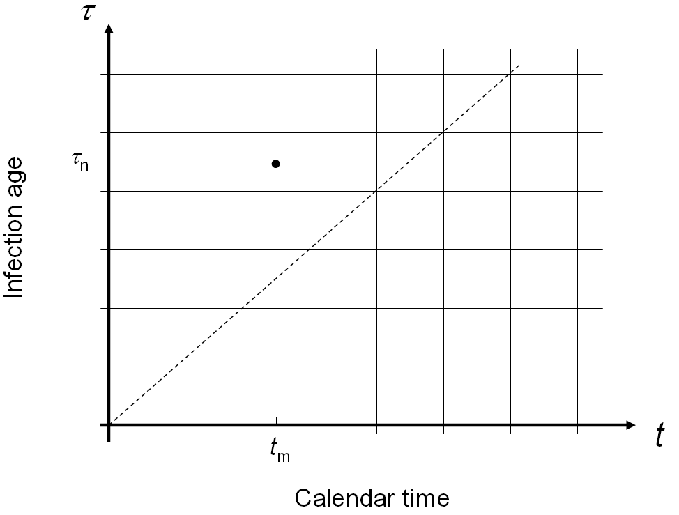
Figure 1: Rectangular grid representing calendar time $t$ (abscissa) and infection-age $\tau$ (ordinate). The grid point $(t_{m},\tau_{n})$ above the main diagonal (dashed line) is highlighted.

In case the transmission rate $\beta(t,\tau)$ only depends on calendar time $t,$ i.e., $\beta(t,\tau)=\beta(t),$ the force of infection can be written as

$$\lambda(t)=\beta(t)\,I(t)=\frac{\mathcal{R}(t)\,I(t)}{S(t)\,\int_{0}^{\infty}\,\varGamma(\tau)\mathrm{d}\tau}.$$

Then, System (2) – (4) becomes explicitly dependent on $\mathcal{R}$. This means for given $\mathcal{R},$ the system can be solved, for instance by the algorithm above, such that the resulting effective reproduction number equals the prescribed $\mathcal{R}.$ This is advantageous in situations, when the effective reproduction number $\mathcal{R}$ is known while the transmission rate $\beta$ is not.

Approximation of the age-structured SIR model by the conventional SIR model

The situation described at the end of the last section, when the effective reproduction $\mathcal{R}(t)$ is known instead of the transmission rate $\beta(t,\tau)$, happens quite frequently. Note that there are a variety of methods for estimating $\mathcal{R}$ from a time series of numbers of incident cases, see e.g. [Cor13, Fra07]. The question arises, under which conditions system (2) – (4) can be approximated by a simpler model that explicitly depends on $\mathcal{R}$.

A simpler model related to System (2) – (4) is the conventional SIR model without demography of the background host:

$$\frac{\mathrm{d}S(t)}{\mathrm{d}t} = -\lambda(t)\,S(t)$$ (11)

$$\frac{\mathrm{d}I(t)}{\mathrm{d}t} = \lambda(t)\,S(t)-r(t)\,I(t)$$ (12)

$$\frac{\mathrm{d}R(t)}{\mathrm{d}t} = r(t)\,I(t)$$ (13)

Using Leibniz’ integral rule and Eq. (5), the temporal derivative $\frac{\mathrm{d}I}{\mathrm{d}t}$ of the number of infected from Eq. (1) can be expressed as

$$\frac{\mathrm{d}I(t)}{\mathrm{d}t} = \frac{\mathrm{d}}{\mathrm{d}t}\int_{0}^{\infty}i(t,\tau)\mathrm{d}\tau=\int_{0}^{\infty}\frac{\partial}{\partial t}i(t,\tau)\mathrm{d}\tau$$ (14)

$$= -\int_{0}^{\infty}\gamma(\tau)\,i(t,\tau)\mathrm{d}\tau-\int_{0}^{\infty}\frac{\partial}{\partial\tau}i(t,\tau)\mathrm{d}\tau$$

$$= -\int_{0}^{\infty}\gamma(\tau)\,i(t,\tau)\mathrm{d}\tau-i(t,\infty)+i(t,0).$$

As $i(t,\infty)=0$ (see above) and $i(t,0)=\lambda(t)\,S(t)$, Eq. (14) reads as

$$\frac{\mathrm{d}I(t)}{\mathrm{d}t}=-\int_{0}^{\infty}\gamma(\tau)\,i(t,\tau)\mathrm{d}\tau+\lambda(t)\,S(t).$$ (15)

It is reasonable to assume that the integral in Eq. (15) has a finite upper bound $\omega<\infty$, because there are no infected people with infinite infection-age. As $i(t,\tau)\geq 0,$ the Mean Value Theorem for Definite Integrals [Has17] guarantees existence of a $\tau^{\star}=\tau^{\star}(t)\in[0,\omega]$ such that

$$\frac{\mathrm{d}I(t)}{\mathrm{d}t}=-\gamma\bigl{(}\tau^{\star}(t)\bigr{)}\,I(t)+\lambda(t)\,S(t).$$ (16)

So far, we could show that Eq. (3) from the age-structured SIR model can be approximated by Eq. (12) with $r(t)=\gamma(\tau^{\star}(t))$. If we can furthermore show that

$$\lambda\,S=\mathcal{R}\,r\,I,$$ (17)

we can reformulate Eq. (12) with an explicit dependency on $\mathcal{R}$. Assumed Eq. (17) holds true, we find

$$\frac{\mathrm{d}I(t)}{\mathrm{d}t} = -r(t)\,I(t)+\mathcal{R}(t)\,r(t)\,I(t)$$ (18)

$$= r(t)\,\bigl{(}\mathcal{R}(t)-1\bigr{)}\,I(t).$$

With the usual smoothness assumptions, Eq. (18) has the unique solution

$$I(t)=I(0)\,\exp\left(\int_{0}^{t}\Bigl{[}r(\sigma)\,\bigl{(}\mathcal{R}(\sigma)-1\bigl{)}\Bigr{]}\mathrm{d}\sigma\right),$$ (19)

where $I(0)=\int_{0}^{\infty}i_{0}(\tau)\mathrm{d}\tau$ (note that $i_{0}$ was assumed to be integrable).

Apart from their simplicity, Eqs. (18) and (19) allow the common interpretation of the effective reproduction number $\mathcal{R}$: the number $I(t)$ of infected increases if and only if $\mathcal{R}(t)>1.$

We have to examine the conditions such that Eq. (17) holds true. As $i(t,\cdot)$ is non-negative, the Mean Value Theorem for Definite Integrals applied to the left hand side of Eq. (17) reads as

$$S(t)\,\lambda(t) = S(t)\int_{0}^{\infty}\beta(t,\tau)\,i(t,\tau)\mathrm{d}\tau$$ (20)

$$= S(t)\,\beta(t,\tau^{\ast}(t))\,I(t)$$

for $\tau^{\ast}(t)\in[0,\omega].$

On the right hand side of Eq. (17), we have

$$\mathcal{R}(t)\,I(t)\,r(t)=S(t)\,\beta(t,\tau^{\prime}(t))\,I(t)\,r(t)\,\int_{0}^{\omega^{\prime}}\varGamma(\tau)\mathrm{d}\tau,$$ (21)

where we assumed that $\beta(t,\cdot)\,\varGamma$ has a compact support $[0,\omega^{\prime}]$ and $\tau^{\prime}(t)\in[0,\omega^{\prime}].$

By comparing Eqs. (20) and (21), we see that $r(t)\,\int_{0}^{\omega^{\prime}}\varGamma(\tau)\mathrm{d}\tau=1$ and $\beta(t,\tau^{\ast}(t))=\beta(t,\tau^{\prime}(t))$ implies $\lambda\,S=\mathcal{R}\,r\,I.$ Hence, for practical purposes if $r(t)=\gamma(\tau^{\star}(t))$ is close to $(\int_{0}^{\omega^{\prime}}\varGamma(\tau)\mathrm{d}\tau)^{-1}$, we can expect that Eq. (19) is a reasonable approximation for the number $I(t)$ of infected in the age-structured SIR model.

Example

We calculate the incidence-density $i$ on the grid $(t_{m},\tau_{n})=(m\times\delta_{h},n\times\delta_{h}),~{}m=0,\dots,M,~{}n=0,\dots,N,$ starting with $(t_{0},\tau_{0})=(0,0)$, ending with $(t_{M},\tau_{N})=(40,30)$ and equidistant stepsize $\delta_{h}=\tfrac{1}{24}$ (in units days). The transmission rate $\beta(t,\tau)$ is assumed to be the product of two Gaussian functions:

$$\beta(t,\tau)=\nu_{0}\times\Bigl{(}\nu_{1}+\nu_{2}\,\exp\bigl{(}-\bigl{[}(t-12)/4\bigr{]}^{2}/2\bigr{)}\Bigr{)}\times\Bigl{(}\exp\bigl{(}-\bigl{[}(\tau-5)/1.5\bigr{]}^{2}/2\bigr{)}\Bigr{)},$$

where $\nu_{0}=5\times 10^{-6},\nu_{1}=1,\nu_{2}=3.$ The removal rate $\gamma$ is assumed to be constant $\gamma(\tau)=\tfrac{1}{8}$. The initial distribution $i_{0}$ is assumed to be $i_{0}(\tau)=20\times\varGamma(\tau),$ where $\varGamma$ is defined in Eq. (9) with $\gamma(\tau)=\tfrac{1}{8}$. Figure 2 shows the resulting incidence-density $i(t,\tau)$ calculated with the Algorithm of the previous section.

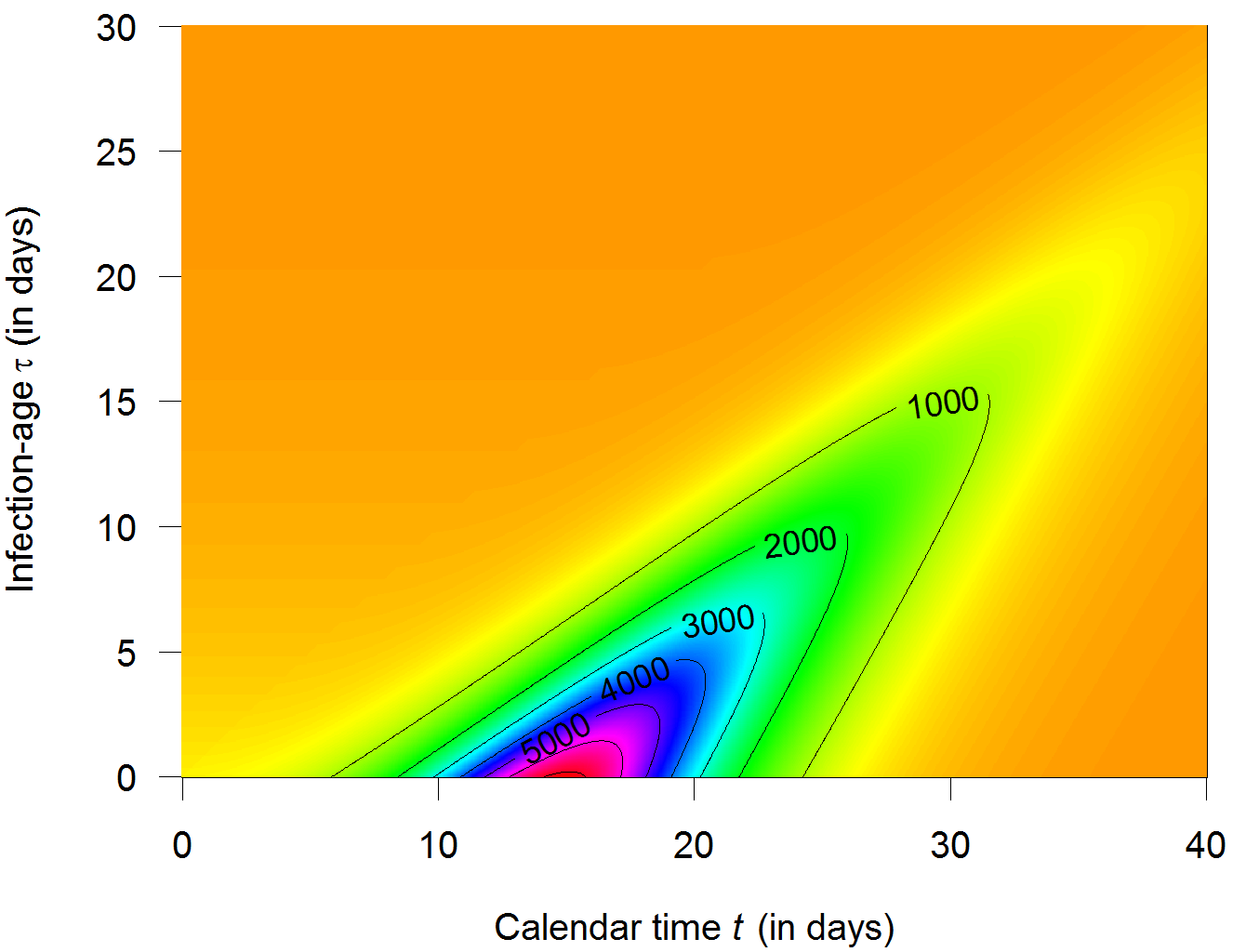
Figure 2: Incidence-density $i(t,\tau)$ in the numerical example.

The resulting reproduction number $\mathcal{R}$ as calculated by Eq. (10) is depicted in Figure 3. If we try to approximate $I$ using $\mathcal{R}$ directly by Eq. (19), we obtain the graph as presented in Figure 4. The black curve corresponds to the approximated $I$ according to Eq. (19) with constant $r(t)=0.1125$. For comparison, the exact $I$ calculated by (1) is shown as blue curve. Although little effort has been spend to optimize the fit between the exact and approximate $I$, the approximation is reasonably well.

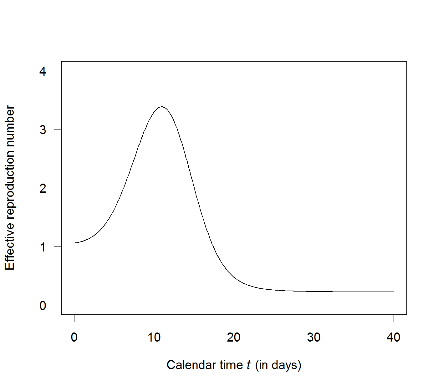
Figure 3: Reproduction number $\mathcal{R}$ (ordinate) over calendar time $t$ in the example.

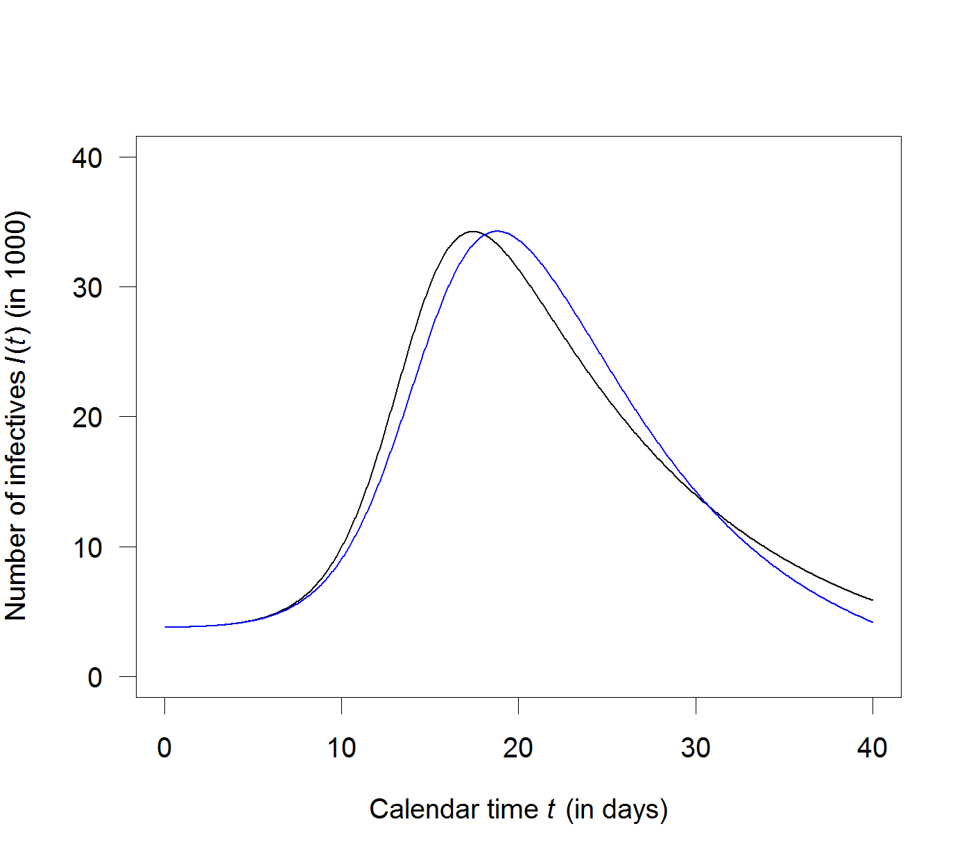
Figure 4: Number $I$ of infectives (ordinate) over calendar time $t$ in the example. The blue curve corresponds to the exact solution (Eq. (1)) while the black curve is the approximation via Eq. (19).

Contact:
<firstname>.<lastname>@stat.uni-muenchen.de
Ludwigstr. 33
D-80539 München
Germany

References

[Che16]
Chen Y, Zou S, Yang J (2016) Global Analysis of an SIR Epidemic Model
with Infection Age and Saturated Incidence, Nonlin Ana: Real World App 30: 16-31.
[Cor13]
Cori A, Ferguson NM, Fraser C, Cauchemez S (2013) A new framework
and software to estimate time-varying reproduction numbers during epidemics.
Amer J Epidem 178(9), 1505-1512.
[Fra07]
Fraser C (2007) Estimating Individual and Household Reproduction Numbers
in an Emerging Epidemic. PLoS ONE 2(8): e758.
[Ina17]
Inaba H (2017) Age-structured Population Dynamics in Demography
and Epidemiology, Springer, Singapore.
[Ker27]
Kermack WO, McKendrick AG (1927) Contributions to the Mathematical
Theory of Epidemics, Proc Royal Soc 115A, 700-21.
[Nis09]
Nishiura H, Chowell G (2009) The Effective Reproduction Number as a Prelude to
Statistical Estimation of Time-Dependent Epidemic Trends, in: Chowell G,
Hyman JM, Bettencourt LMA, Castillo-Chavez C: Mathmatical and Statistical
Estimation Approaches in Epidemiology, Springer, Dordrecht.