A Flexible Framework for Designing Trainable Priors with Adaptive Smoothing and Game Encoding

Abstract

We introduce a general framework for designing and training neural network layers whose forward passes can be interpreted as solving non-smooth convex optimization problems, and whose architectures are derived from an optimization algorithm. We focus on convex games, solved by local agents represented by the nodes of a graph and interacting through regularization functions. This approach is appealing for solving imaging problems, as it allows the use of classical image priors within deep models that are trainable end to end. The priors used in this presentation include variants of total variation, Laplacian regularization, bilateral filtering, sparse coding on learned dictionaries, and non-local self similarities. Our models are fully interpretable as well as parameter and data efficient. Our experiments demonstrate their effectiveness on a large diversity of tasks ranging from image denoising and compressed sensing for fMRI to dense stereo matching.

1 Introduction

Despite the undeniable successes of deep learning in domains as varied as image processing [63] and recognition [21], natural language processing [10], speech [43] or bioinformatics [1], feed-forward neural networks are often maligned as being “black boxes” that, except perhaps for their top classification or regression layers, are difficult or even impossible to interpret. In imaging applications, for example, the elementary operations typically consist of convolutions and pointwise nonlinearities, with many parameters adjusted by backpropagation, and no obvious functional interpretation.

In this paper, we consider instead network architectures explicitly derived from an optimization algorithm, and thus interpretable from a functional point of view. The first instance of this approach we are aware of is LISTA [20], which provides a fast approximation of sparse coding. Yet, we are not content to design an architecture that provides a fast approximation to a given optimization problem, but we also want to learn a data representation pertinent for the corresponding task. This yields an unusual machine learning paradigm, where one learns the parameters of a parametric objective function used to represent data, while designing an optimization algorithm to minimize it efficiently.

Even though interpretability is not always necessary to achieve good prediction, this point of view, sometimes called algorithm unrolling [17, 40], has proven successful for solving inverse imaging problems, providing effective and parameter-efficient models. This approach allows the use of domain-specific priors within trainable deep models, leading to a large number of applications such as compressive imaging [53, 62], demosaicking [26], denoising [26, 50, 52], and super-resolution [56] .

However, existing approaches are often limited to simple image priors such as sparsity induced by the $\ell_{1}$-norm [52], or differentiable regularization functions [27], and a general algorithmic framework for combining complex, possibly non-smooth, regularization functions is still missing. Our paper addresses this issue and is able to leverage a large class of image priors such as total variation [49], the $\ell_{1}$-norm, structured sparse coding [34], or Laplacian regularization, where local optimization problems interact with each others. The interaction can be local among direct neighbors on an image grid, or non-local, capturing for instance similarities between spatially distant image patches [5, 12].

In this context, we adopt a more general and flexible point of view than the standard convex optimization paradigm, and consider formulations to represent data based on non-cooperative games [42] potentially involving non-smooth terms, which are tackled by using the Moreau-Yosida regularization technique [22, 61]. Unrolling the resulting optimization algorithm results in a network architecture that can be trained end-to-end and capture any combination of the domain-specific priors mentioned above. This approach includes and improves upon specific trainable sparse coding models based on the $\ell_{1}$-norm for example [52, 56]. More importantly perhaps, it can be used to construct several interesting new image priors: In particular, we show that a trainable variant of total variation and its non-local variant based on self similarities is competitive with the state of the art in imaging tasks, despite using up to 50 times fewer parameters, with corresponding gains in speed. We demonstrate the effectivness and the flexibility of our approach on several imaging tasks, namely denoising, compressed fMRI reconstruction, and stereo matching.

Summary of our contributions.

First, we provide a new framework for building trainable variants of a large class of domain-specific image priors. Second, we show that several of these priors match or even outperform existing techniques that use a much larger number of parameters and training data. Finally, we present a set of practical tricks to make optimization-driven layers easy to train.

2 Background and Related Work

Classical image priors.

Inverse imaging problems are often solved by minimizing a data fitting term with respect to model parameters, regularized with a penalty that encourages solutions with a particular structure. In image processing, the community long focused on designing handcrafted priors such as sparse coding on learned dictionaries [14, 33], diffusion operators [45], total variation [49], and non-local self similarities [5], which is a key ingredient of successful restoration algorithms such as BM3D [12]. However these methods are now often outperformed by deep learning models [29, 63, 64], which leverage pairs of corrupted/clean training images in a supervised fashion.

Bilevel optimization.

A simple method for mixing data representation learning with optimization is to use a bi-level formulation [32]. For instance, assuming that one is given pairs $(\mathbf{x}_{i},\mathbf{y}_{i})_{i=1\dots n}$ of corrupted/clean signals with $\mathbf{x}_{i}$ and $\mathbf{y}_{i}$ in $\mathbb{R}^{m}$, one may consider the following bi-level objective

$$\min_{\boldsymbol{\theta}\in{\Theta},\mathbf{W}\in\mathbb{R}^{m\times p}}\frac{1}{n}\sum_{i=1}^{n}L(\mathbf{y}_{i},\mathbf{W}\mathbf{z}^{\star}_{\boldsymbol{\theta}}(\mathbf{x}_{i}))~{}~{}~{}~{}\text{where}~{}~{}~{}~{}\mathbf{z}^{\star}_{\boldsymbol{\theta}}(\mathbf{x}_{i})\in\operatorname*{arg\,min}_{\mathbf{z}\in\mathbb{R}^{p}}h_{\boldsymbol{\theta}}(\mathbf{x}_{i},\mathbf{z}),$$ (1)

where $\boldsymbol{\theta}$ is a set of model parameters, $\mathbf{W}\mathbf{z}^{\star}_{\boldsymbol{\theta}}(\mathbf{x}_{i})$ is a prediction which is compared to $\mathbf{y}_{i}$ through a loss function $L:\mathbb{R}^{m}\times\mathbb{R}^{m}\rightarrow\mathbb{R}^{+}$, and the data representation $\mathbf{z}_{\boldsymbol{\theta}}^{\star}(\mathbf{x}_{i})$ in $\mathbb{R}^{p}$ is obtained by minimizing some function $h_{\boldsymbol{\theta}}$. Note that for simplicity, we have considered here a multivariate regression problem, where given a signal $\mathbf{x}$ in $\mathbb{R}^{m}$, we want to predict another signal $\mathbf{y}$ in $\mathbb{R}^{m}$, but this formulation also applies to classification problems. It was first introduced for sparse coding in [32, 58] and it has recently been extended to the case when $\mathbf{z}^{\star}_{\boldsymbol{\theta}}(\mathbf{x}_{i})$ is replaced by an approximate minimizer of $h_{\boldsymbol{\theta}}$.

Unrolled algorithms.

A common approach to solving (1) consists in choosing an iterative method for minimizing $h_{\boldsymbol{\theta}}$ and then define  $\mathbf{z}^{\star}_{\boldsymbol{\theta}}(\mathbf{x}_{i})$ as the output of the optimization method after $K$ iterations. The sequence of operations performed by the optimization method can be seen as a computational graph and $\nabla_{\boldsymbol{\theta}}\mathbf{z}_{\boldsymbol{\theta}}^{\star}$ can be computed by automatic differentiation. This often yields neural-network-like computational graphs, which we call optimization-driven layers. Such architectures have found multiple applications such as training of conditional random fields [65], stabilization of generative adversarial networks [38], structured prediction [3], or hyper-parameters tuning [31]. For image restoration, various optimization problems have been explored including for example sparse coding [26, 52, 62], non linear diffusion [9] and differential operator regularization [27]. Many inference algorithms have been investigated including proximal gradient descent [27, 52], ADMM [17], half quadratic spliting [66], or augmented Lagrangian [48].

3 A General Framework for Learning Optimization-Driven Layers

3.1 Proposed Approach

We adopt a more general point of view than (1), where we assume that input signals admit a local “patch” structure (e.g., rectangular image regions) and the data representation encodes individual patches. Assuming that there are $m$ patches in $\mathbf{x}$, we denote by $\mathbf{Z}^{\star}(\mathbf{x})=[\mathbf{z}_{1}^{\star}(\mathbf{x}),\ldots,\mathbf{z}_{m}^{\star}(\mathbf{x})]$ in $\mathbb{R}^{p\times m}$ the representation of $\mathbf{x}$ and by $\mathbf{z}_{j}^{\star}(\mathbf{x})$ the representation of patch $j$ (we omit the dependency on the model parameters $\boldsymbol{\theta}$ for simplicity). In imaging applications and as in previous models [52], $\mathbf{Z}^{\star}(\mathbf{x})$ can be seen as a feature map akin to that of a convolutional neural network with $p$ channels.

Figure 1: Our models encode locally an input feature vector. The local optimal solutions $\mathbf{z}_{j}^{\star}$ interact trough the regularization function $\psi_{\theta}^{j}(\mathbf{Z})$.

Encoding with non-cooperative convex games.

Concretely, given a signal $\mathbf{x}$, we denote by $\mathbf{P}_{j}\mathbf{x}$ the patch of $\mathbf{x}$ centered at position $j$, where $\mathbf{P}_{j}$ is a linear patch extraction operator, and we define the optimal encoding $\mathbf{Z}^{\star}(\mathbf{x})$ of $\mathbf{x}$ as a Nash equilibrium of the set of problems

$$\min_{\mathbf{z}_{j}\in{\mathcal{Z}}}h_{\boldsymbol{\theta}}(\mathbf{P}_{j}\mathbf{x},\mathbf{z}_{j})+\psi_{\boldsymbol{\theta}}^{j}(\mathbf{Z})~{}~{}~{}~{}\text{for}~{}~{}j=1,\ldots,m,$$ (2)

where $h_{\boldsymbol{\theta}}$ is a a convex reconstruction objective for each patch, parametrized by $\boldsymbol{\theta}$, $\psi_{\boldsymbol{\theta}}^{j}$ is a convex regularization function encoding interactions between the variable $\mathbf{z}_{j}$ and the remaining ones $\mathbf{z}_{l}$ for $l\neq j$, and $\mathcal{Z}$ is a convex subset of $\mathbb{R}^{p}$. When $\mathcal{Z}$ is compact, the problem is a specific instance of a non-cooperative convex game [42], which is known to admit at least one Nash equilibrium—that is, a solution such that one of the objectives in (2) is optimal with respect to its variable $\mathbf{z}_{j}$ when the other variables $\mathbf{z}_{l}$ for $l\neq j$ are fixed. The conditions under which an optimization algorithm is guaranteed to return such an equilibrium point are well studied, see Section 3.3, and in many situations the compactness of $\mathcal{Z}$ is not required, as also observed in our experiments where we choose $\mathcal{Z}=\mathbb{R}^{p}$. For instance, in several practical cases, (2) can be solved by minimizing the sum of $m$ convex terms, a setting called a potential game, which boils down to a classical convex optimization problem.

3.2 Application of our Framework to Inverse Imaging Problems

In this section, we show how to leverage our optimization-driven layers for imaging. For the sake of clarity we choose to narrow down the scope of this presentation to imaging, even though our method is not limited to this single application: different modalities including for example genomic/graph data could benefit from our methodology.

Examples of models $h_{\boldsymbol{\theta}}$.

We consider two cases in the rest of this presentation:

• Pixel reconstruction: $h_{\boldsymbol{\theta}}(\mathbf{P}_{j}\mathbf{x},\mathbf{z}_{j})=(\mathbf{x}_{j}-\mathbf{z}_{j})^{2}$, where $\mathbf{x}_{j}$ is the pixel $j$ of $\mathbf{x}$ and $\mathbf{z}_{j}$ is a scalar, corresponding to patches of size $q=1\times 1$ and $p=1$.

• Patch encoding on a dictionary: $h_{\boldsymbol{\theta}}(\mathbf{P}_{j}\mathbf{x},\mathbf{z}_{j})=\|\mathbf{P}_{j}\mathbf{x}_{j}-\mathbf{D}\mathbf{z}_{j}\|^{2}$, where $\mathbf{D}$ in $\mathbb{R}^{q\times p}$ is a dictionary, $q$ is the patch size, and $p$ is the number of dictionary elements. This is a classical model where patch $j$ is approximated by a linear, often sparse, combination of dictionary elements [14].

Only the second choice involves model parameters $\mathbf{D}$ (represented by $\boldsymbol{\theta}$). These two loss functions are common in image processing [14], but other losses may be used for other modalities.

Linear reconstruction with a dictionary.

Assuming that $\mathbf{y}$ and $\mathbf{x}$ have the same size $m$ for simplicity, predicting $\mathbf{y}$ from a feature map $\mathbf{Z}^{\star}(\mathbf{x})$ is typically achieved by using a learned dictionary matrix $\mathbf{W}$ in $\mathbb{R}^{q\times p}$ where $q$ is the patch size. Then, $\mathbf{W}\mathbf{z}_{j}^{\star}(\mathbf{x})$ can be interpreted as a reconstruction of the $j$-patch of $\mathbf{y}$ . Since the patches overlap, we obtain $q$ estimators for every pixel, which can be combined by averaging (neglecting border effects below for simplicity), yielding the prediction

$$\hat{\mathbf{y}}(\mathbf{x},\theta,\mathbf{W})=\frac{1}{q}\sum_{j=1}^{m}\mathbf{P}_{j}^{\top}\mathbf{W}\mathbf{z}^{\star}_{j}(\mathbf{x}),$$ (3)

where $\mathbf{P}_{j}^{\top}$ is the linear operator that places a patch of size $q$ at position $j$ in a signal of dimension $m$. Patch averaging is a classical operation in patch-based image restoration algorithms, see [14], which can be interpreted in terms of transposed convolution and admits fast implementations on GPUs.

Learning problem.

For image restoration, given training pairs of corrupted/clean images $\{\mathbf{x}_{i},\mathbf{y}_{i}\}_{i=1,\ldots,n}$, we consider the regression problem $\min_{\boldsymbol{\theta}\in\Theta,\mathbf{W}\in\mathbb{R}^{q\times p}}\|\mathbf{y}_{i}-\hat{\mathbf{y}}(\mathbf{x}_{i},\theta,\mathbf{W})\|^{2}~{}~{}~{}~{}\text{where}~{}~{}\hat{\mathbf{y}}(\mathbf{x}_{i})~{}~{}\text{is defined in~{}(\ref{eq:averaging})}$.

Figure 2: Architecture of our trainable models for image restoration.

Examples of regularization functions $\psi_{\boldsymbol{\theta}}^{j}$.

Our framework allows the use of several regularization functions, which are presented in the table 1 below. We assume that the patches are nodes in a graph, and denote by ${\mathcal{N}}_{j}$ the set of neighbors of the patch $j$. For natural images, the graph may be a two-dimensional grid with edge weights $a_{j,k}$ that depend on the relative position of the patches $j$ and $k$, which we denote by $a_{j\text{--}k}$, but it may also be a non-local graph based on some similarity function as in [26, 29]. Concretely, we can consider:

• the distance $d^{j,k}_{\mathrm{NL}}=\|\operatorname{diag}(\boldsymbol{\kappa})(\mathbf{P}_{j}\mathbf{x}-\mathbf{P}_{k}\mathbf{x})\|^{2}$ between patches $j$ and $k$ of the image $\mathbf{x}$, where $\boldsymbol{\kappa}$ in $\mathbb{R}^{q}$ is a set of parameters to learn, and $q$ is the patch size, and we define normalized weights $a_{\mathrm{NL}}^{j,k}={e^{-d^{j,k}_{\mathrm{NL}}}}/{\sum_{l\in\mathcal{N}_{j}}e^{-d^{j,k}_{\mathrm{NL}}}}$.

• or a distance inspired from the bilateral filter [54]. In that case we define the distance $d^{j,k}_{\mathrm{BL}}=\frac{\|\mathbf{x}_{i}-\mathbf{x}_{j}\|^{2}}{2\sigma_{d}^{2}}+\frac{\|i-j\|^{2}}{2\sigma_{r}^{2}}$ between pixels on a local window $\mathcal{N}_{j}$ centered around pixel $j$, and we define again normalized weights $a_{\mathrm{BL}}^{j,k}={e^{-d^{j,k}_{\mathrm{BL}}}}/{\sum_{l\in\mathcal{N}_{j}}e^{-d^{j,k}_{\mathrm{BL}}}}$.

Table 1: A non-exhaustive list of regularization functions $\psi_{\boldsymbol{\theta}}$ covered by our framework.

	$\psi_{\boldsymbol{\theta}}^{j}(\mathbf{Z})$	Model parameters
Laplacian	$\sum_{k\in{\mathcal{N}}_{j}}a_{j\text{--}k}\|\mathbf{z}_{j}-\mathbf{z}_{k}\|^{2}$	weights in $\mathbb{R}^{|{\mathcal{N}}|}$
Non-local Laplacian	$\sum_{k\in{\mathcal{N}}_{j}}a_{\mathrm{NL}}^{j,k}\|\mathbf{z}_{j}-\mathbf{z}_{k}\|^{2}$	$\boldsymbol{\kappa}$ in $\mathbb{R}^{q}$
Bilateral filter (BF)	$\sum_{k\in{\mathcal{N}}_{j}}a_{\mathrm{BL}}^{j,k}\|\mathbf{z}_{j}-\mathbf{z}_{k}\|^{2}$	$\sigma_{d}\in\mathbb{R}$ and $\sigma_{r}\in\mathbb{R}$
Total variation (TV)	$\sum_{k\in{\mathcal{N}}_{j}}a_{j\text{--}k}\|\mathbf{z}_{j}-\mathbf{z}_{k}\|_{1}$	weights in $\mathbb{R}^{|{\mathcal{N}}|}$
Non-local total variation (NLTV)	$\sum_{k\in{\mathcal{N}}_{j}}a_{\mathrm{NL}}^{j,k}\|\mathbf{z}_{j}-\mathbf{z}_{k}\|_{1}$	$\boldsymbol{\kappa}$ in $\mathbb{R}^{q}$
Bilateral TV (BLTV)	$\sum_{k\in{\mathcal{N}}_{j}}a_{\mathrm{BL}}^{j,k}\|\mathbf{z}_{j}-\mathbf{z}_{k}\|_{1}$	$\sigma_{d}\in\mathbb{R}$ and $\sigma_{r}\in\mathbb{R}$
Weighted $\ell_{1}$-norm (sparse coding)	$\sum_{l=1}^{p}\lambda_{l}|\mathbf{z}_{j}[l]|$	$\boldsymbol{\lambda}$ in $\mathbb{R}^{p}$
Non-local group regularization	$\sum_{l=1}^{p}\lambda_{l}\sqrt{\sum_{k\in{\mathcal{N}}_{j}}a_{j,k}\mathbf{z}_{k}[l]^{2}}$	$\boldsymbol{\lambda}$ in $\mathbb{R}^{p}$ and $\boldsymbol{\kappa}$ in $\mathbb{R}^{q}$
Variance reduction	$\|\mathbf{W}\mathbf{z}_{j}-\mathbf{P}_{j}\hat{\mathbf{y}}\|^{2}$ with $\hat{\mathbf{y}}$ from (3)	$\mathbf{W}$ from (3)

Novelty of the proposed formulation and relation to previous work.

• Total variation: to the best of our knowledge, the basic anisotropic TV penalty [6] does not seem to appear in the literature on unrolled algorithms with end-to-end training. Note also that our TV variant allows learning non-symmetric weights $a_{j,k}\neq a_{k,j}$, leading to a non-cooperative game that goes beyond the classical convex optimization framework typically used with the TV penalty.

• Non-local TV: the non-local TV penalty presented above is based on a classical formulation [19], but can be incorporated within a trainable deep network with non-symmetric weights.

• Bilateral filtering: the bilateral filter and its TV variant implemented in this paper are based on classical formulations [54, 16]. But they have not, to the best of our knowledge, been implemented as trainable priors.

• Sparse coding and variance reduction: the weighted $\ell_{1}$-norm combined with the patch encoding loss $h_{\boldsymbol{\theta}}$ yields a sparse coding formulation (SC) that has been well studied within optimization-driven layers [50, 52]. Yet, the codes $\mathbf{z}_{j}$ in the SC setup are obtained by solving independent optimization problems, which has motivated by Simon and Elad [52] to propose instead a Convolutional Sparse Coding model (CSC), where the full image is approximated by a linear combination of small dictionary elements. Unfortunately, as noted in [52], CSC leads to ill-conditioned optimization problems, making a hybrid approach between SC and CSC more effective. Our paper proposes an alternative solution combining the weighted $\ell_{1}$-norm regularization with a variance reduction penalty, which forces the codes $\mathbf{z}_{j}$ to reach a consensus when reconstructing the image $\hat{\mathbf{y}}$. Our experiments show that this approach outperforms [52] for image denoising.

• Non-local group regularization: This regularization function corresponds to a soft variant of the Group Lasso penalty [55], which encourages similar patches to share similar sparsity patterns (set of non-zero elements of the codes $\mathbf{z}_{j}$). It was originally used in [34] and was recently revisited within optimization-driven layers with an heuristic algorithm [26]. Our paper provides a better justified algorithmic framework as well as the ability to combine this penalty with other ones.

Algorithm 1 Pseudocode of the general training procedure for image restoration

1:Sample a minibatch of pairs of corrupted/clean images $\{(\mathbf{x}_{0},\mathbf{y}_{0}),\cdots,(\mathbf{x}_{K},\mathbf{y}_{K})\}$;

2:Extract overlapping patches of corrupted images to form tensors $\mathbf{X}_{i}=[\mathbf{P}_{1}\mathbf{x}_{i},\cdots,\mathbf{P}_{n}\mathbf{x}_{i}]$;

3:for $t=1,2,\ldots,K$ do $\triangleright$ Compute an approximate Nash equilibrium $\mathbf{Z}^{\star}$ of the convex games

4:     $\mathbf{Z}_{t+1}\leftarrow\mathbf{Z}_{t}-\eta_{t}H_{\theta}(\mathbf{Z}_{t},\mathbf{X})$;

5:end for

6:Approximate clean images by linear reconstruction $\hat{\mathbf{y}}=\frac{1}{q}\sum_{j=1}^{m}\mathbf{P}_{j}^{\top}\mathbf{W}\mathbf{z}^{\star}_{j}(\mathbf{X},\theta)$;

7:Compute the $\ell_{2}$ reconstruction loss $\|\mathbf{y}-\hat{\mathbf{y}}(\mathbf{x},\theta,\mathbf{W})\|_{2}^{2}$ on the minibatch;

8:Compute an estimate of the gradients wrt. $(\theta,\mathbf{W})$ with auto-diff;

9:Update trainable parameters $(\theta,\mathbf{W})$ with Adam;

3.3 Differentiability and End-to-end Training

In this section we adress end-to-end training of the optimization-driven layers. Given pairs of training data $\{\mathbf{x}_{i},\mathbf{y}_{i}\}_{i=1,\ldots,n}$, we consider the learning problem

$$\min_{\boldsymbol{\theta}\in{\Theta}}\frac{1}{n}\sum_{i=1}^{n}L\left(\mathbf{y}_{i},g_{\theta}\left(\mathbf{z}^{\star}_{\boldsymbol{\theta}}(\mathbf{x}_{i})\right)\right),$$ (4)

where $g_{\theta}$ is a differentiable function. We consider the approximation where the codes $\mathbf{z}_{j}^{\star}(\mathbf{x})$ are obtained as the $K$-th step of an optimization algorithm for solving the problem (2). To obtain these codes, we leverage (i) iterative gradient and extra-gradient methods, which are classical for solving game problems [4, 15], and (ii) a smoothing technique for dealing with the regularization functions $\psi_{\boldsymbol{\theta}}^{j}$ above when they are non-smooth. Refer to Algorithm 1 for an overview of the training procedure. We start with the first point when dealing with smooth objectives.

Unrolled optimization for convex games.

Consider a set of $m$ objective functions of the form

$$\min_{\mathbf{z}_{j}\in\mathbb{R}^{p}}h_{j}(\mathbf{Z})~{}~{}~{}~{}\text{with}~{}~{}~{}~{}\mathbf{Z}=[\mathbf{z}_{1},\ldots,\mathbf{z}_{m}],$$ (5)

where the functions $h_{j}$ are convex and differentiable and may depend on other parameters than $\mathbf{z}_{j}$. Our objective is to find a zero of the simultaneous gradient

$$H(\mathbf{Z})=[\nabla_{\mathbf{z}_{1}}h_{1}(\mathbf{Z}),\cdots,\nabla_{\mathbf{z}_{m}}h_{m}(\mathbf{Z})],$$ (6)

which corresponds to a Nash equilibrium of the game (5). In the rest of this presentation, we consider both the general setting and the simpler case of so-called potential games, for which the equilibrium can be found as the optimum of a single convex objective. This is the case for several of our regularizers, for example the TV penalty with symmetric weights. More details are provided in Appendix A on the nature of the non-cooperative games corresponding to our penalties.

Two standard methods studied in the variational inequality litterature [4, 15, 23, 37] are the gradient and the extra-gradient [25] methods. The iterates of the basic gradient method are given by

$$\mathbf{Z}_{t+1}=\mathbf{Z}_{t}-\eta_{t}H(\mathbf{Z}_{t}),$$ (7)

where $\eta_{t}>0$ is a step-size. These iterates are known to converge under a condition called strong monotonicity of the operator $H$, which is related to the concept of strong convexity in optimization, see [4]. Because this condition is relatively stringent, the extra-gradient method is often prefered [25], as it is known to converge under weaker conditions, see [23, 37]. The intuition of the method is to compute a look ahead step in order to compute more stable directions of descent:

$$\begin{split}\text{Extrapolation step}\quad&\mathbf{Z}_{t+1/2}=\mathbf{Z}_{t}-\eta_{t}H(\mathbf{Z}_{t})\\ \text{Update step}\quad&\mathbf{Z}_{t+1}=\mathbf{Z}_{t}-\eta_{t}H(\mathbf{Z}_{t+1/2}).\end{split}$$ (8)

In this paper, our strategy is to unroll iterates of one of these two algorithms, and then to use auto differentiation for learning the model parameters $\boldsymbol{\theta}$. Furthermore, parameters that control the optimization process (e.g., step size $\eta_{t}$) can also be learnt with this approach. It should be noted that optimization-driven layers have never been used before in the context of non-cooperative games, to the best of our knowledge, and therefore an empirical study is needed to choose between the strategies (7) or (8). In our experiments, extra-gradient descent has always performed at least as well, and sometimes significantly better, than plain gradient descent for comparable computational budgets. See for example Table 2 for a smoothed variant of the TV penalty.

Table 2: Gradient descent (GD) vs. Extra-gradient. Denoising results in avg. PSNR with $\sigma=25$ on BSD68 [35].

Method	GD (24 iters)	GD (48 iters)	Extra-gradient (24 iters)
Trainable TV symmetric	27.58	27.50	27.82
Trainable TV assymetric	27.99	27.89	28.24

Moreau-Yosida smoothing.

The non-smooth regularization functions we consider can be written as a sum of simple terms. Omitting the dependency on $\boldsymbol{\theta}$ for simplicity, we may indeed write

$$\psi^{j}(\mathbf{Z})=\textstyle\sum_{k=1}^{r}\phi_{k}(L_{k,j}(\mathbf{Z}))~{}~{}~{}~{}\text{for some}~{}r\geq 1,$$

where $L_{k,j}$ is a linear mapping and $\phi_{k}$ is either the $\ell_{1}$- or $\ell_{2}$-norm. For instance, $\phi_{k}$ is the $\ell_{1}$-norm with $L_{k,j}(\mathbf{Z})=a_{k,j}(\mathbf{z}_{j}-\mathbf{z}_{k})$ in $\mathbb{R}^{p}$ for the TV penalty, and $L_{k,j}(\mathbf{Z})=[\sqrt{a_{1,j}}\mathbf{z}_{1}(k),\ldots,\sqrt{a_{1,j}}\mathbf{z}_{q}(k)]^{\top}$ in $\mathbb{R}^{q}$ with $\phi_{k}$ being the $\ell_{2}$-norm for the non-local group regularization. Handling such non-smooth convex terms may be achieved by leveraging the so-called Moreau-Yosida regularization [28, 41, 60]

$$\Phi_{k}(\mathbf{u})=\min_{\mathbf{v}}\left\{\phi_{k}(\mathbf{v})+\frac{\alpha}{2}\|\mathbf{v}-\mathbf{u}\|^{2}\right\},$$

which defines an optimization problem whose solution is called the proximal operator $\text{Prox}_{\phi_{k}/\alpha}[\mathbf{u}]$. As shown in [28], $\Phi_{k}$ is always differentiable and $\nabla\Phi_{k}(\mathbf{u})=\alpha(\mathbf{u}-\text{Prox}_{\phi_{k}/\alpha}[\mathbf{u}])$, which can be computed in closed form when $\phi_{k}=\ell_{1}$ or $\ell_{2}$. The positive parameter $\alpha$ controls the trade-off between smoothness (the gradient of $\Phi_{k}$ is $\alpha$-Lipschitz) and the quality of approximation. It is thus natural to define a smoothed approximation $\Psi^{j}$ of $\psi^{j}$ as $\Psi^{j}(\mathbf{Z})=\sum_{k=1}^{r}\Phi_{k}(L_{k,j}(\mathbf{Z}))$.

Note that when the proximal operator of $\psi^{j}$ can be computed efficiently, as is the case for the $\ell_{1}$-norm, gradient descent algorithms can typically be adapted to handle the non-smooth penalty without extra computational cost [33], and there is no need for Moreau-Yosida smoothing. However, the proximal operator of the TV penalty and the non-local group regularization do not admit fast implementations. For the first one, computing the proximal operator requires solving a network flow problem [7], whereas the second one is essentially easy to solve when the weights $a_{j,k}$ form non-overlapping groups of variables, leading to a penalty called group Lasso [55].

We are now ready to present our unrolled algorithm as we have previously discussed gradient-based algorithms for solving convex smooth games and a smoothing technique for handling non-smooth terms. Generally, at iteration $t$, the gradient algorithm (7) performs the following simultaneous updates for all problems $j$

$$\begin{split}\mathbf{u}_{k,j}^{(t)}~{}~{}~{}&\leftarrow\operatorname{\text{Prox}}_{\phi_{k}/\alpha_{k,t}}[L_{k,j}(\mathbf{Z}^{(t)})]~{}~{}~{}~{}~{}~{}\text{for}~{}~{}k=1,\ldots,r\\ \mathbf{z}_{j}^{(t+1)}&\leftarrow\mathbf{z}_{j}^{(t)}-\eta_{t}\left(\nabla_{\mathbf{z}_{j}}h_{\theta}\left(\mathbf{P}_{j}\mathbf{x},\mathbf{z}_{j}^{(t)}\right)+\sum_{k=1}^{r}\alpha_{k,t}\>\left[L_{k,j}^{*}\left(L_{k,j}(\mathbf{Z}^{(t)})-\mathbf{u}_{k,j}^{(t)}\right)\right]_{j}\right),\\ \end{split}$$

where $L_{k,j}^{*}$ is the adjoint of the linear mapping $L_{k,j}$. The computation of the gradients can be implemented with simple operations allowing auto-differentiation in deep learning frameworks. Interestingly, the smoothing parameter $\alpha$ can be made iteration-dependent, and learned along with other model parameters such that the amount of smoothing is chosen automatically.

3.4 Tricks of the Trade for Unrolled Optimization

Our strategy is to unroll iterates of our algorithms, and then compute $\nabla_{\boldsymbol{\theta}}\mathbf{z}_{\boldsymbol{\theta}}^{\star}$ by automatic differentiation. We present here a set of practical rules, some old and some new, facilitating training when $h_{\boldsymbol{\theta}}$ is a patch encoding function on a dictionary $\mathbf{D}$.

Initialization.

To help the algorithm converge, we choose an initial stepsize $\eta_{t}\leq\frac{1}{L}$, where $L$ is the Lipschitz constant of $\nabla_{\mathbf{z}}h_{\boldsymbol{\theta}}$, which is the classical step-size used by ISTA [2]. To do so, inspired by [52] we normalize the initial dictionary by its largest singular value and take $\eta_{0}=1$. Note that we can go one step further and normalize the dictionary throughout the training phase. This is in fact equivalent to the spectral normalization that has received some attention recently, notably for generative adversarial networks [39].

Untied parameters.

In our framework, $\nabla_{\mathbf{z}_{j}}h_{\boldsymbol{\theta}}(\mathbf{P}_{j}\mathbf{x},\mathbf{z}_{j})=\mathbf{D}^{\top}\left(\mathbf{D}\mathbf{z}_{j}-\mathbf{P}_{j}\mathbf{x}\right)$. It has been suggested in previous work [20, 26, 52] to introduce an additional parameter $\mathbf{C}$ of the same size as $\mathbf{D}$, and consider instead the parametrization $\mathbf{C}^{\top}\left(\mathbf{D}\mathbf{z}_{j}-\mathbf{P}_{j}\mathbf{x}\right)$, $\mathbf{C}$ acting as a learned preconditioner. Even though the theoretical effect of this modification is not fully understood, it has been observed to accelerate convergence and boost performance for denoising tasks [26]. In our experiments, we will indicate in which cases we use this heuristic.

Backtracking.

A simple way for handling the potential instability of the unrolled algorithm is to use a backtracking scheme which automatically decreases the stepsize when the training loss diverges. This heuristic was used for instance in [26]. More details are provided in Appendix B.

Barzilai-Borwein method for choosing the stepsize.

A different, perhaps more principled, approach to improved stability consists in adaptively choosing an adaptive stepsize $\eta_{t}$. The literature on convex optimization proposes a set of effective rules, known as Barzilai-Borwein (BB) step size rules [57]. Even though these rules were not designed for convex games, they appear to be very effective in practice in the context of our optimization-driven layers. Concretely, they lead to step sizes $\eta_{t,j}={\|\mathbf{D}^{\top}\mathbf{D}\mathbf{s}_{j}\|_{2}}/{\|\mathbf{D}\mathbf{s}_{j}\|^{2}}$ with ${\mathbf{s}}_{j}=\mathbf{z}_{j}^{(t)}-\mathbf{z}_{j}^{(t-1)}$ for problem $j$ at iteration $t$.

Table 3: Study of stabilization techniques for learnt sparse coding. Denoising results in average PSNR with $\sigma=25$ on BSD68.

Method	Psnr (dB)
	D	C,D
BM3D [11]	28.57
Sparse Coding (SC)	✗	✗
SC + Backtracking	28.71	28.83
SC + Spectral norm	28.69	28.82
SC + Barzilai-Borwein	28.82	28.86

In our experiments, we observed that spectral normalization, backtracking, and Barzilai-Borwein step size were all effective to stabilize training. We have noticed that the spectral normalization impacts negatively the reconstruction accuracy, while the BB method tend to improve it by using larger stepsizes, at the expense of a larger computational cost. This is illustrated in Table 3 for a smoothed variant of sparse coding (we indicate with a crossmark when the algorithm diverges). In addition, we observe that the untied models brings a small boost in reconstruction accuracy.

4 Experiments

We consider three different tasks, illustrated with various combinations of regularization functions in order to demonstrate the wide applicability of our approach and its flexibility. A software package and additional details are provided in the supplementary material for reproducibility purposes.

Table 4: Grayscale denoising on BSD68, training on BSD400 for all methods. Performance in terms of average PSNR. Tiny CNN is a CNN baseline with few parameters. See Appendix C for qualitative results.

Method	Params	Noise Level ($\sigma$)
		5	15	25	50
Tiny CNN (ours)	326	35.17	29.42	26.90	24.06
Tiny CNN (ours)	1200	36.47	30.36	27.70	24.60
BM3D [11]	-	37.57	31.07	28.57	25.62
LSCC [34]	-	37.70	31.28	28.71	25.72
CSCnet [52]	62k	37.69	31.40	28.93	26.04
GroupSC [26]	68k	37.95	31.71	29.20	26.17
FFDNet [64]	486k	N/A	31.63	29.19	26.29
DnCNN [63]	556k	37.68	31.73	29.22	26.23
NLRN [29]	330k	37.92	31.88	29.41	26.47
Pixel-reconstruction
TV symmetric	288	36.91	30.27	27.66	24.51
TV assymetric - extra-grad	480	37.30	30.76	28.24	25.32
Laplacian symmetric	288	35.17	28.42	26.14	23.70
Laplacian assymetric - extra-grad	480	35.20	28.46	26.39	23.77
Bilateral - extra-grad	146	36.75	29.89	27.20	23.72
Bilateral TV - extra-grad	146	36.94	30.46	27.78	24.52
Non-local TV - extra-grad	307	37.53	31.03	28.50	25.26
Non-local Laplacian - extra-grad	307	37.54	31.00	28.47	25.46
Patch-reconstruction
Sparse Coding (SC)	68k	37.84	31.46	28.90	25.84
Sparse Coding + Variance	68k	37.83	31.49	29.00	26.08
Sparse Coding + TV	68k	37.84	31.50	29.02	26.10
Sparse Coding + TV + Variance	68k	37.84	31.51	29.03	26.09
Non-local group	68k	37.95	31.69	29.19	26.19
Non-local group + Variance	68k	37.96	31.70	29.22	26.28
GroupSC + Variance	68k	37.96	31.75	29.24	26.34

Image denoising.

For image denoising experiments, we use the standard setting of [63] with BSD400 [35] as a training set and on BSD68 as a test set. We optimize the parameters of our models using Adam [24] and also use the backtracking strategy described in Section 3.4 that automatically decreases the learning rate by a factor 0.5 when the training loss diverges. For the non-local models, we follow [26] and update the similarity matrices three times during the inference step. We use the parametrization with the $\mathbf{C}$ matrix for our patch-based experiments. We also combine our variance regularization with [26]. Additional training details and hyperparameters choices can be found in Appendix B. We report performance in terms of averaged PSNR in Table 4, and more detailed tables with additional results are available in Appendix C for pixel-level models, and for the patch-based models involving a dictionary $\mathbf{D}$. Our models based on non-local sparse approximations perform better than the competing deep learning models with the exception of [29] for $\sigma\geq 15$ with much fewer parameters. In addition, we also observed that our assymetric TV models are almost on par with BM3D while being significantly faster (see Appendix C for more details) with only a very small amount of parameters.

Compressed Sensing for fMRI.

Compressed Sensing for functional magnetic resonance imaging (fMRI) aims at reconstructing functional MR images from a small number of samples in the Fourier space. The corresponding inverse problem is

$$\min_{\mathbf{y}\in\mathbb{R}^{n}}\|\mathbf{A}\mathbf{y}-\mathbf{x}\|^{2}_{2}+\lambda\Psi(\mathbf{y}),$$ (9)

where the degradation matrix is $\mathbf{A}=\mathbf{P}\mathcal{F}$, $\mathbf{P}$ is a diagonal binary sampling matrix for a given sub-sampling pattern, $\mathcal{F}$ is the discrete Fourier transform such that the observed corrupted signal $\mathbf{x}$ is in the Fourier domain, and $\Psi$ is a regularization function. This problem highlights the ability of our framework to handle both localized and non localized constraints. In our paper, we implemented two models revisiting some well studied priors for compressed sensing in an end-to-end fashion:

• Pixel reconstruction with total variation: we aim at solving the optimization for each node $\min_{\mathbf{y}_{i}\in\mathbb{R}}\left\|\mathbf{A}\mathbf{y}-\mathbf{x}\right\|_{2}^{2}+\text{TV}_{i}(\mathbf{y})$. In the past, total variation has been widely used for MRI [30], often in combination with sparse regularization in the wavelet domain.

• Patch encoding on a dictionary with sparse coding: we solve a collection of optimization problems of the form $\min_{\mathbf{z}_{i}\in\mathbb{R}^{n}}\left\|\mathbf{A}\hat{\mathbf{y}}(\mathbf{z})-\mathbf{x}\ \right\|_{2}^{2}+\lambda\|\mathbf{z}_{i}\|_{1}$, with ${\mathbf{y}}=\frac{1}{n}\sum_{j}\mathbf{R}_{j}^{\top}\mathbf{D}\mathbf{z}_{j}$ the average of the overlapping patches. Some previous methods have explored dictionary-based reconstruction [47], but they were not investigated from a task-driven manner with end-to-end training.

In our experiments, we use the same setting as [53] for fair comparison: we train and test our models on the brain MRI dataset studied in that paper. Our models are trained separately for each sampling rate. We used the pseudo radial sampling for the matrix $\mathbf{P}$ similarly to the other methods. The reconstruction accuracy are reported in term of PSNR over the test set in Table 5. Our trainable model relying on a trainable TV prior performs surprisingly well given the conceptual simplicity of the prior. Also importantly, it runs significantly faster than all competing methods with a very small number of parameters. Furthermore, our trainable sparse coding method for fMRI gives strong performance and exceeds the state of the art for sampling rates larger than 30%. Note that architecture choices (patch and dictionary size) of our models are the same as for the denoising task, and we did not try to optimize them for the considered task, thus demonstrating the robustness of our approach.

Table 5: Compressed sensing for fMRI on the MR brain dataset using a pseudo radial sampling pattern. Performance comparisons in terms of PSNR (dB).

Method	Params	20 %	30 %	40%	50%	Test time
TV [30]	-	35.20	37.99	40.00	41.69	0.731s (cpu)
RecPF [59]	-	35.32	38.06	40.03	41.71	0.315s (cpu)
SIDWT	-	35.66	38.72	40.88	42.67	7.867s (cpu)
PANO [46]	-	36.52	39.13	40.31	41.81	35.33s (cpu)
BM3D-MRI [13]	-	37.98	40.33	41.99	43.47	40.91s (cpu)
ADMM-net [53]	-	37.17	39.84	41.56	43.00	0.791s (cpu)
ISTA-net [62]	337k	38.73	40.89	42.52	44.09	0.143s (gpu)
CS-TV (ours)	140	36.80	39.63	41.58	43.46	0.015s (gpu)
CS-Sparse coding (ours)	68k	37.80	40.50	42.46	44.16	0.213s (gpu)
CS-Sparse coding + Variance (ours)	68k	37.79	40.67	42.54	44.17	0.213s (gpu)

Table 6: Denoising with less data. Results in terms of average PSNR(dB) on BSD68 with $\sigma=15$. All the models are trained on a similar subset of BSD400 for fair comparaison.

Method	Params	Training images
		400	200	100	50
DnCNN [63]	556k	31.73	31.65	31.47	31.23
TV extra-grad	480	30.75	30.72	30.67	30.66
SC+Var	68k	31.49	31.49	31.47	31.40
GroupSC+Var	68k	31.75	31.66	31.62	31.54

Table 7: Dense stereo matching fine-tuning on kitti2015 train set, performance reported on the kitti2015 validation set.

Model	3-px error (%)
PSMNet [8]	2.14 $\pm$ 0.04
PSMNet+TV 12	2.11 $\pm$ 0.03
PSMNet+TV 24	2.11 $\pm$ 0.04
PSMNet+TV extra	2.10 $\pm$ 0.03

Dense Stereo Matching.

Our approach can be used to provide a generic regularization module that can easily be integrated into various neural architectures. We showcase its versatility by using it for deep stereo matching [51]. Given aligned image pairs, the goal is to compute disparity $\bf d$ for each pixel. Traditionally stereo matching is formulated as minimization of an energy function $E_{\text{data}}(\mathbf{d})+\lambda E_{\text{smooth}}(\mathbf{d})$ where the data term, $E_{\text{data}}$ measures how well $\mathbf{d}$ agrees with the input image pairs, $E_{\text{smooth}}$ enforces consistency among neighboring pixels’ disparities: TV is a commonly chosen regularizer. Recent deep learning methods tackle the problem as a supervised regression to estimate continuous disparity map given pairs of stereo views and ground truth disparity maps [8]. We propose to combine our smoothing TV block with a state-of-the-art deep learning model [8]. In practice, we combine our block with a pretrained model on the SceneFlow [36] dataset, and fine-tune the pretrained model on the kitti2015 [18] train set, following the training procedure described in [8]. We used the original implementation of [8] available online and did not change any hyperparameters. We report in Table 4 the performance on the validation set in term of 3 pixels error which counts predicted pixel as correct if the disparity deviates from the ground truth from 3 pixels or less. We ran the experiment 10 times for each model (with and without the TV regularization). We observed that our TV block introduces very few additional parameters and consistently boosts performances.

Training with few examples.

We conducted denoising experiments with less training data and report corresponding results in Table 6. We use the code released by the authors for training DnCNN with less data. Very interestingly the gap between our best model and CNN-based models increases when decreasing the size of the training set. We believe that this is an appealing feature, particularly relevant for applications in medical imaging or microscopy where the amount of training data can be very limited.

5 Discussion

We have presented a general framework based on non-cooperative games to train end-to-end imaging priors. Our experiments demonstrate the flexibility and the effectiveness of our approach on diverse tasks ranging from image denoising to fMRI reconstruction and dense stereo matching. Beyond image processing, we believe that the issue of interpretability is important. We consider models with a clear mathematical description of the decision function they produce. As a by-product, our models are also more parameter efficient than classical deep learning models. We believe that these are important steps to build systems that should not be seen as black boxes anymore, that produce explanable decisions, and that do not require training a system for days on a huge corpus of annotated data. These are important questions, which we are planning to address explicitly in the future.

Broader Impact

Our main field of application is in image processing, with a focus on image restoration and reconstruction, whose benefits for society are clear and well established, even though a misuse of such a technology is of course possible; for instance, the same total variation penalty may be used in medical imaging, for personal photography, in astronomical imaging, or for restoring images produced by military devices. More specifically, our paper is addressing the issue of interpretability of neural networks, by considering models admitting a functional (mathematical) description of their decision functions, and with less parameters than classical deep learning models. As we mentioned in the discussion section, we believe that these are first steps to build systems producing explanable decisions, and that are more data and energy efficient. These are important issues going beyond image processing, which we would like to address in future work.

Appendix

This supplementary material is organized as follows: In Section A, we discuss additional priors that were not presented in the main paper, but which are in principle compatible with our framework, and we provide more details about potential games. In Section B, we provide implementation details that are useful to reproduce the results of our paper (note that the code is also provided). In Section C, we present additional quantitative results and additional results regarding inference speed of our models that were not included in the main paper for space limitation reasons. Finally, in Section D, we present additional qualitative results (which require zooming on a computer screen).

Appendix A Discussion on Models and Priors

A.1 Additional Priors

Our framework makes it possible to handle models of the form:

$$h_{j}(\mathbf{Z})=h_{\boldsymbol{\theta}}(\mathbf{P}_{j}\mathbf{x}_{j},\mathbf{z}_{j})+\lambda\sum_{k=1}^{r}\phi_{k}(L_{k,j}(\mathbf{Z})),$$ (10)

where $\phi_{k}$ is a simple convex function that admits a proximal operator in closed form, and $L_{k,j}$ is a linear operator. In the main paper, several regularization functions have been considered, including the total variation, variance reduction, or non-local group regularization penalties. Here, we would like to mention a few additional ones, which are in principle compatible with our framework, but which we did not investigate experimentally. In particular, two of them may be of particular interest, and may be the topic of future work:

• the regularization $\lambda\|\mathbf{H}^{\top}\mathbf{z}_{j}\|_{1}$, where $\mathbf{H}$ is a matrix, may correspond to several settings. The matrix $\mathbf{H}$ may be for instance a wavelet basis, or may by learned, corresponding then to the penalty used in the analysis dictionary learning model from the paper “The cosparse analysis model and algorithms” of Nam et al., 2013.

• the regularization $\lambda\phi(\mathbf{H}^{\top}\mathbf{z}_{j})$ where $\phi$ is a smooth function is closely related to the model introduced in [27], and to the Field of experts model of Roth and Black from the 2005 paper “Fields of Experts: A Framework for Learning Image Priors”, even though the functions used in these other works are not convex.

A.2 Potential Games

A potential game is a non-cooperative convex game whose Nash equilibria correspond to the solutions of a convex optimization problem. We will now consider problems of the form (10), and show that all penalties that admit some symmetry are in fact potential games. Assuming the functions $\phi_{k}$ to be smooth for simplicity, optimality conditions for the convex problems (10) are, for all $j=1,\ldots,m$:

$$\nabla_{\mathbf{z}_{j}}h_{\boldsymbol{\theta}}(\mathbf{P}_{j}\mathbf{x}_{j},\mathbf{z}_{j})+\lambda\sum_{k=1}^{r}\nabla_{\mathbf{z}_{j}}\tilde{\phi}_{k,j}(\mathbf{Z})=0,~{}~{}~{}~{}\text{with}~{}~{}~{}~{}\tilde{\phi}_{k,j}(\mathbf{Z})={\phi}_{k}(L_{k,j}(\mathbf{Z})).$$ (11)

Let us now assume the following symmetry condition such that if problem $l$ involves a variable $\mathbf{z}_{j}$ through a function $\tilde{\phi}_{k,l}(\mathbf{Z})$, then problem $j$ also involves the same term. Based on this assumption, we may define the potential function

$$V(\mathbf{Z}):=\sum_{j=1}^{m}\left(h_{\boldsymbol{\theta}}(\mathbf{P}_{j}\mathbf{x}_{j},\mathbf{z}_{j})+\frac{\lambda}{2}\sum_{k=1}^{r}\tilde{\phi}_{k,j}(\mathbf{Z})\right).$$

The partial derivative of this potential function with respect to $\mathbf{z}_{j}$ is then

$$\nabla_{\mathbf{z}_{j}}h_{\boldsymbol{\theta}}(\mathbf{P}_{j}\mathbf{x}_{j},\mathbf{z}_{j})+\frac{\lambda}{2}\sum_{l=1}^{m}\sum_{k=1}^{r}\nabla_{\mathbf{z}_{j}}\tilde{\phi}_{k,l}(\mathbf{Z})=\nabla_{\mathbf{z}_{j}}h_{\boldsymbol{\theta}}(\mathbf{P}_{j}\mathbf{x}_{j},\mathbf{z}_{j})+\frac{\lambda}{2}\sum_{l=1}^{m}\sum_{k\in\mathcal{N}_{j,l}}\nabla_{\mathbf{z}_{j}}\tilde{\phi}_{k,l}(\mathbf{Z}),$$

where $\mathcal{N}_{j,l}$ is the set of functions $\tilde{\phi}_{k,l}$ involving variable $\mathbf{z}_{j}$. The previous gradient can then be simplified into

$$\nabla_{\mathbf{z}_{j}}h_{\boldsymbol{\theta}}(\mathbf{P}_{j}\mathbf{x}_{j},\mathbf{z}_{j})+\frac{\lambda}{2}\sum_{j=1}^{r}\nabla_{\mathbf{z}_{j}}\tilde{\phi}_{k,l}(\mathbf{Z})+\frac{\lambda}{2}\sum_{l\neq j}\sum_{k\in\mathcal{N}_{j,l}}\nabla_{\mathbf{z}_{j}}\tilde{\phi}_{k,l}(\mathbf{Z}).$$

Since the symmetry condition can be expressed as $\sum_{j=1}^{r}\tilde{\phi}_{k,l}(\mathbf{Z})=\sum_{l\neq j}\sum_{k\in\mathcal{N}_{j,l}}\tilde{\phi}_{k,l}(\mathbf{Z})$, the condition $\nabla V(\mathbf{Z})=0$ is then equivalent to (11). Note that we have assumed the functions $\phi_{k}$ to be smooth for simplicity, but a similar reasoning can be conducted for non-smooth functions, by using the concept of subgradients.

Examples of potential games.

• the $\ell_{1}$-norm: with $r=1$ and $\tilde{\phi}_{1,j}=\|\mathbf{z}_{j}\|_{1}$, since problem $j$ does not involve any variable $\mathbf{z}_{l}$ for $l\neq j$;

• Symmetric TV / Laplacian: problem $j$ may involve a variable $\mathbf{z}_{l}$ through a term $a_{j,l}\|\mathbf{z}_{j}-\mathbf{z}_{l}\|_{1}$. Then, problem $l$ involves the same term $a_{l,j}\|\mathbf{z}_{j}-\mathbf{z}_{l}\|_{1}$ under the condition $a_{j,l}=a_{l,j}$.

• Symmetric non local group with $r=p$ and $\tilde{\phi}_{k,j}=\lambda_{k}\|[\sqrt{a_{j,1}}\mathbf{z}_{1}(k),\ldots,\sqrt{a_{j,m}}\mathbf{z}_{m}(k)]^{\top}\|_{2}$. Under the condition of symmetric weights $a_{j,l}=a_{l,j}$, we obtain again a potential game.

Potential games are appealing as they provide guarantees about the existence of Nash equilibria without requiring optimizing over a compact set. Yet, we have found that allowing non-symmetric weights often performs better. This is illustrated in Table A1 for a simple denoising experiment.

Table A1: Symmetric vs assymmetric grayscale denoising on BSD68, training on BSD400 for all methods. Performance is measured in terms of average PSNR.

Method	Params	Noise Level ($\sigma$)
		5	15	25	50
TV symmetric	72	36.08	30.21	27.58	24.74
TV assymetric - extra-grad	480	37.30	30.76	28.24	25.32
Laplacian symmetric	72	34.88	28.14	25.90	23.45
Laplacian assymetric - extra-grad	480	35.20	28.46	26.39	23.77
Non-local group - symmetric	68k	37.94	31.67	29.17	26.16
Non-local group - assymetric	68k	37.95	31.69	29.20	26.19

Appendix B Implementation Details and Reproducibility

B.1 Training Details

For the training of patch-based models for denoising, we randomly extract patches of size $56\times 56$ whose size equals the window size used for computing non-local self-similarities; whereas we train pixel level models on the full size images. For fMRI experiments we also trained the models on the full sized images. We apply a mild data augmentation (random rotation by $90^{\circ}$ and horizontal flips). We optimize the parameters of our models using ADAM [24].

The learning rate is set to $6\times 10^{-4}$ at initialization and is sequentially lowered during training by a factor of 0.35 every 80 training steps, in the same way for all experiments. Similar to [52], we normalize the initial dictionary $\mathbf{D}_{0}$ by its largest singular value as explained in the main paper in Section 3.4. We initialize the dictionary $\mathbf{C}$,$\mathbf{D}$ and $\mathbf{W}$ with the same dictionary obtained with an unsupervised dictionary learning algorithm (using SPAMS library).

We have implemented the backtracking strategy described in Section 3.4 of the main paper for all our algorithms, which automatically decreases the learning rate by a factor 0.8 when the loss function increases too much on the training set, and restore a previous snapshot of the model. Divergence is monitored by computing the loss on the training set every 10 epochs. Training the non-local models for denoising are the longer models to train and takes about 2 days on a Titan RTX GPU. We summarize the chosen hyperparameters for the experiments in Table A2.

Table A2: Hyper-parameters chosen for every task.

Experiment	Gray denoising (patch)	Gray denoising (pixel)	fMRI
Patch size	9	-	9
Dictionary size	256	-	256
Nr epochs	300	300	150
Batch size	32	32	1
$K$ iterations	24	24	24
Middle averaging	✓	✓	-
Correlation update frequency $f$	${1}/{6}$	$1/12$	-

Appendix C Additional Quantitative Results

C.1 Inference speed

In Table A3 we provide a comparison of our TV models in terms of speed with BM3D for grayscale denoising on the BSD68 dataset. For fair comparison, we reported computation time both on gpu and cpu.

Table A3: Inference speed for image denoising.

	Params	Psnr	Speed
BM3D [11]	-	25.62	7.28s (cpu)
TV assymetric	240	24.93	0.014s (gpu) / 0.18s (cpu)
TV assymetric (extra)	480	25.32	0.021s (gpu) / 0.28s (cpu)

C.2 Image denoising

We provide additional results for grayscale denoising with different variations of the prior introduced in the main paper, as well as combination of different priors. We reported performances for gray denoising in Table A4 for the pixel based models, and in Table A5 for the patch based models. In Table A4 untied $\kappa$ denotes when we used a different set of learned parameters $\kappa$ at each stage of the refinement step of the similarity matrix for the non-local models.

Table A4: Pixel level grayscale denoising on BSD68, training on BSD400 for all models. Performance is measured in terms of average PSNR.

Method	Params	Noise Level ($\sigma$)
		5	15	25	50
BM3D [11]	-	37.57	31.07	28.57	25.62
Tiny CNN	326	35.17	29.42	26.90	24.06
Tiny CNN	1200	36.47	30.36	27.70	24.60
TV symmetric	288	36.08	30.21	27.58	24.74
TV symmetric - extra-grad	144	37.02	30.33	27.82	24.81
TV assymetric-	240	36.83	30.49	27.99	24.93
TV assymetric - extra-grad	480	37.30	30.76	28.24	25.32
Laplacian symmetric	288	34.88	28.14	25.90	23.45
Laplacian symmetric - extra-grad	144	33.87	28.14	25.91	23.45
Laplacian assymetric	240	35.20	28.48	26.17	23.78
Laplacian assymetric - extra-grad	480	35.20	28.46	26.39	23.77
Non-local TV assymmetric	154	37.25	30.86	28.28	25.42
Non-local TV assymmetric (untied $\kappa$)	235	37.12	31.01	28.37	25.24
Non-local TV assymmetric - extra-grad	226	37.83	30.98	28.34	25.31
Non-local TV assymmetric - extra-grad (untied $\kappa$)	307	37.53	31.03	28.50	25.26
Non-local Laplacian assymmetric	154	37.31	30.75	28.33	25.15
Non-local Laplacian assymmetric (untied $\kappa$)	235	37.53	31.01	28.37	25.47
Non-local Laplacian assymmetric - extra-grad	226	37.51	30.99	28.34	25.13
Non-local Laplacian assymmetric - extra-grad (untied $\kappa$)	307	37.54	31.00	28.47	25.46
Bilateral	74	36.76	29.89	27.16	23.97
Bilateral TV	74	36.60	29.82	27.23	24.00
Bilateral - extra-grad	146	36.75	29.89	27.20	23.72
Bilateral TV - extra-grad	146	36.94	30.46	27.78	24.52

Table A5: Patch level grayscale denoising on BSD68, training on BSD400 for all methods. Performance is measured in terms of average PSNR.

Method	Params	Noise Level ($\sigma$)
		5	15	25	50
BM3D [11]	-	37.57	31.07	28.57	25.62
LSCC [34]	-	37.70	31.28	28.71	25.72
CSCnet [52]	62k	37.69	31.40	28.93	26.04
FFDNet [64]	486k	N/A	31.63	29.19	26.29
DnCNN [63]	556k	37.68	31.73	29.22	26.23
NLRN [29]	330k	37.92	31.88	29.41	26.47
GroupSC [26]	68k	37.95	31.71	29.20	26.17
Sparse Coding + Barzilai-Borwein	68k	37.85	31.46	28.91	25.84
Sparse Coding + Variance	68k	37.83	31.49	29.00	26.08
Sparse Coding + TV	68k	37.84	31.50	29.02	26.10
Sparse Coding + TV + Variance	68k	37.84	31.51	29.03	26.09
Sparse Coding + TV + Variance + Barzilai-Borwein	68k	37.86	31.52	29.04	26.04
Non-local group - symmetric	68k	37.94	31.67	29.17	26.16
Non-local group - assymetric	68k	37.95	31.69	29.20	26.19
Non-local group - assymetric + TV	68k	37.96	31.71	29.22	26.26
Non-local group - assymetric + Variance	68k	37.96	31.70	29.23	26.28
Non-local group - assymetric + Variance + TV	68k	37.95	31.71	29.24	26.30
GroupSC + Variance	68k	37.96	31.75	29.24	26.34

Appendix D Additional Qualitative Results

Finaly, we show qualitative results for grayscale denoising in Figures A3, A4.

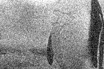
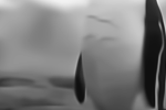
	ground truth	noisy	BM3D
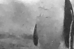
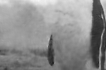
	TV (ours)	NLTV (ours)	NL-Lap (ours)
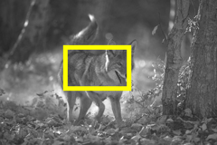
	ground truth	noisy	BM3D
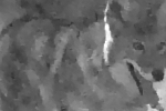
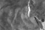
	TV	NLTV (ours)	NL-Lap (ours)
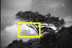
	ground truth	noisy	BM3D
	TV (ours)	NLTV (ours)	NL-Lap (ours)
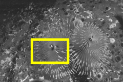
	ground truth	noisy	BM3D
	TV(ours)	NLTV (ours)	NL-Lap local (ours)

Figure A3: Grayscale denoising for 4 images from the BSD68 dataset. Best seen by zooming on a computer screen.

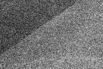
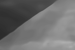
	ground truth	noisy	BM3D
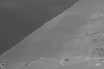
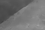
	DnCNN	SC (ours)	Non local (ours)
	ground truth	noisy	BM3D
	DnCNN	SC (ours)	Non local (ours)
	ground truth	noisy	BM3D
	DnCNN	SC (ours)	Non local (ours)
	ground truth	noisy	BM3D
	DnCNN	SC (ours)	Non local (ours)

Figure A4: Results of our patch level models for grayscale denoising for 4 images from the BSD68 dataset. Best seen by zooming on a computer screen.

References

- [1] B. Alipanahi, A. Delong, M. T. Weirauch, and B. J. Frey. Predicting the sequence specificities of dna-and rna-binding proteins by deep learning. Nature biotechnology, 33(8):831–838, 2015.
- [2] A. Beck and M. Teboulle. A fast iterative shrinkage-thresholding algorithm for linear inverse problems. SIAM journal on Imaging Sciences, 2(1):183–202, 2009.
- [3] D. Belanger, B. Yang, and A. McCallum. End-to-end learning for structured prediction energy networks. In Proc. International Conference on Machine Learning (ICML), 2017.
- [4] D. P. Bertsekas and J. N. Tsitsiklis. Parallel and distributed computation: numerical methods. Prentice hall Englewood Cliffs, NJ, 1989.
- [5] A. Buades, B. Coll, and J.-M. Morel. A non-local algorithm for image denoising. In Proc. Conference on Computer Vision and Pattern Recognition (CVPR), 2005.
- [6] A. Chambolle, V. Caselles, D. Cremers, M. Novaga, and T. Pock. An introduction to total variation for image analysis. Theoretical foundations and numerical methods for sparse recovery, 9(263-340):227, 2010.
- [7] A. Chambolle and J. Darbon. On total variation minimization and surface evolution using parametric maximum flows. International journal of computer vision, 84(3):288, 2009.
- [8] J.-R. Chang and Y.-S. Chen. Pyramid stereo matching network. In Proc. Conference on Computer Vision and Pattern Recognition (CVPR), pages 5410–5418, 2018.
- [9] Y. Chen and T. Pock. Trainable nonlinear reaction diffusion: A flexible framework for fast and effective image restoration. IEEE Transactions on Pattern Analysis and Machine Intelligence, 39(6):1256–1272, 2016.
- [10] R. Collobert and J. Weston. A unified architecture for natural language processing: Deep neural networks with multitask learning. In Proc. International Conference on Machine Learning (ICML), 2008.
- [11] K. Dabov, A. Foi, V. Katkovnik, and K. Egiazarian. Image denoising by sparse 3-D transform-domain collaborative filtering. IEEE Transactions on Image Processing, 16(8):2080–2095, 2007.
- [12] K. Dabov, A. Foi, V. Katkovnik, and K. Egiazarian. BM3D image denoising with shape-adaptive principal component analysis. In Proceedings of SPARS’09, Signal Processing wiht Adaptive Sparse Structured Representations, 2009.
- [13] E. M. Eksioglu. Decoupled algorithm for mri reconstruction using nonlocal block matching model: Bm3d-mri. Journal of Mathematical Imaging and Vision, 56(3):430–440, 2016.
- [14] M. Elad and M. Aharon. Image denoising via sparse and redundant representations over learned dictionaries. IEEE Transactions on Image processing, 15(12):3736–3745, 2006.
- [15] F. Facchinei and J.-S. Pang. Finite-dimensional variational inequalities and complementarity problems. Springer Science & Business Media, 2007.
- [16] S. Farsiu, D. Robinson, M. Elad, and P. Milanfar. Advances and challenges in super-resolution. International Journal of Imaging Systems and Technology, 14(2):47–57, 2004.
- [17] A. K. Fletcher, P. Pandit, S. Rangan, S. Sarkar, and P. Schniter. Plug-in estimation in high-dimensional linear inverse problems: A rigorous analysis. In Adv. in Neural Information Processing Systems (NeurIPS), 2018.
- [18] A. Geiger, P. Lenz, and R. Urtasun. Are we ready for autonomous driving? the kitti vision benchmark suite. In 2012 IEEE Conference on Computer Vision and Pattern Recognition, pages 3354–3361. IEEE, 2012.
- [19] G. Gilboa and S. Osher. Nonlocal operators with applications to image processing. Multiscale Modeling & Simulation, 7(3):1005–1028, 2009.
- [20] K. Gregor and Y. LeCun. Learning fast approximations of sparse coding. In Proc. International Conference on Machine Learning (ICML), 2010.
- [21] K. He, X. Zhang, S. Ren, and J. Sun. Deep residual learning for image recognition. In Proc. Conference on Computer Vision and Pattern Recognition (CVPR), 2016.
- [22] J.-B. Hiriart-Urruty and C. Lemaréchal. Convex analysis and minimization algorithms I: Fundamentals, volume 305. Springer science & business media, 2013.
- [23] A. Juditsky, A. Nemirovski, and C. Tauvel. Solving variational inequalities with stochastic mirror-prox algorithm. Stochastic Systems, 1(1):17–58, 2011.
- [24] D. P. Kingma and J. Ba. Adam: A method for stochastic optimization. In Proc. International Conference on Learning Representations (ICLR), 2013.
- [25] G. Korpelevich. The extragradient method for finding saddle points and other problems. Matecon, 12:747–756, 1976.
- [26] B. Lecouat, J. Ponce, and J. Mairal. Fully trainable and interpretable non-local sparse models for image restoration. preprint arXiv:1912.02456, 2020.
- [27] S. Lefkimmiatis. Universal denoising networks: a novel cnn architecture for image denoising. In Proc. Conference on Computer Vision and Pattern Recognition (CVPR), 2018.
- [28] C. Lemaréchal and C. Sagastizábal. Practical aspects of the moreau–yosida regularization: Theoretical preliminaries. SIAM Journal on Optimization, 7(2):367–385, 1997.
- [29] D. Liu, B. Wen, Y. Fan, C. C. Loy, and T. S. Huang. Non-local recurrent network for image restoration. In Adv. in Neural Information Processing Systems (NeurIPS), 2018.
- [30] M. Lustig, D. Donoho, and J. M. Pauly. Sparse mri: The application of compressed sensing for rapid mr imaging. Magnetic Resonance in Medicine: An Official Journal of the International Society for Magnetic Resonance in Medicine, 58(6):1182–1195, 2007.
- [31] D. Maclaurin, D. Duvenaud, and R. Adams. Gradient-based hyperparameter optimization through reversible learning. In Proc. International Conference on Machine Learning (ICML), 2015.
- [32] J. Mairal, F. Bach, and J. Ponce. Task-driven dictionary learning. IEEE Transactions on Pattern Analysis and Machine Intelligence, 34(4):791–804, 2011.
- [33] J. Mairal, F. Bach, J. Ponce, et al. Sparse modeling for image and vision processing. Foundations and Trends in Computer Graphics and Vision, 8(2-3):85–283, 2014.
- [34] J. Mairal, F. R. Bach, J. Ponce, G. Sapiro, and A. Zisserman. Non-local sparse models for image restoration. In Proc. International Conference on Computer Vision (ICCV), 2009.
- [35] D. Martin, C. Fowlkes, D. Tal, J. Malik, et al. A database of human segmented natural images and its application to evaluating segmentation algorithms and measuring ecological statistics. 2001.
- [36] N. Mayer, E. Ilg, P. Häusser, P. Fischer, D. Cremers, A. Dosovitskiy, and T. Brox. A large dataset to train convolutional networks for disparity, optical flow, and scene flow estimation. In IEEE International Conference on Computer Vision and Pattern Recognition (CVPR), 2016. arXiv:1512.02134.
- [37] P. Mertikopoulos, B. Lecouat, H. Zenati, C.-S. Foo, V. Chandrasekhar, and G. Piliouras. Optimistic mirror descent in saddle-point problems: Going the extra (gradient) mile. In Proc. International Conference on Learning Representations (ICLR), 2018.
- [38] L. Metz, B. Poole, D. Pfau, and J. Sohl-Dickstein. Unrolled generative adversarial networks. In Proc. International Conference on Learning Representations (ICLR), 2017.
- [39] T. Miyato, T. Kataoka, M. Koyama, and Y. Yoshida. Spectral normalization for generative adversarial networks. In Proc. International Conference on Learning Representations (ICLR), 2018.
- [40] V. Monga, Y. Li, and Y. C. Eldar. Algorithm unrolling: Interpretable, efficient deep learning for signal and image processing. arXiv preprint arXiv:1912.10557, 2019.
- [41] J. J. Moreau. Fonctions convexes duales et points proximaux dans un espace Hilbertien. CR Acad. Sci. Paris Sér. A Math, 255:2897–2899, 1962.
- [42] H. Nikaidô, K. Isoda, et al. Note on non-cooperative convex games. Pacific Journal of Mathematics, 5(Suppl. 1):807–815, 1955.
- [43] A. v. d. Oord, S. Dieleman, H. Zen, K. Simonyan, O. Vinyals, A. Graves, N. Kalchbrenner, A. Senior, and K. Kavukcuoglu. Wavenet: A generative model for raw audio. arXiv preprint arXiv:1609.03499, 2016.
- [44] A. Paszke, S. Gross, F. Massa, A. Lerer, J. Bradbury, G. Chanan, T. Killeen, Z. Lin, N. Gimelshein, L. Antiga, A. Desmaison, A. Kopf, E. Yang, Z. DeVito, M. Raison, A. Tejani, S. Chilamkurthy, B. Steiner, L. Fang, J. Bai, and S. Chintala. Pytorch: An imperative style, high-performance deep learning library. In Adv. in Neural Information Processing Systems (NeurIPS). 2019.
- [45] P. Perona and J. Malik. Scale-space and edge detection using anisotropic diffusion. IEEE Transactions on Pattern Analysis and Machine Intelligence (PAMI), 12(7):629–639, 1990.
- [46] X. Qu, Y. Hou, F. Lam, D. Guo, J. Zhong, and Z. Chen. Magnetic resonance image reconstruction from undersampled measurements using a patch-based nonlocal operator. Medical image analysis, 18(6):843–856, 2014.
- [47] S. Ravishankar and Y. Bresler. Mr image reconstruction from highly undersampled k-space data by dictionary learning. IEEE transactions on medical imaging, 30(5):1028–1041, 2010.
- [48] Y. Romano, M. Elad, and P. Milanfar. The little engine that could: Regularization by denoising (red). SIAM Journal on Imaging Sciences, 10(4):1804–1844, 2017.
- [49] L. I. Rudin, S. Osher, and E. Fatemi. Nonlinear total variation based noise removal algorithms. Physica D: nonlinear phenomena, 60(1-4):259–268, 1992.
- [50] M. Scetbon, M. Elad, and P. Milanfar. Deep k-svd denoising. arXiv preprint arXiv:1909.13164, 2019.
- [51] D. Scharstein and R. Szeliski. A taxonomy and evaluation of dense two-frame stereo correspondence algorithms. International journal of computer vision, 47(1-3):7–42, 2002.
- [52] D. Simon and M. Elad. Rethinking the CSC model for natural images. Advances in Neural Information Processing Systems (NeurIPS), 2019.
- [53] J. Sun, H. Li, Z. Xu, et al. Deep admm-net for compressive sensing mri. In Adv. in Neural Information Processing Systems (NIPS), 2016.
- [54] C. Tomasi and R. Manduchi. Bilateral filtering for gray and color images. In Proc. International Conference on Computer Vision (ICCV), 1998.
- [55] B. Turlach, W. Venables, and S. Wright. Simultaneous variable selection. Technometrics, 47(3):349, 2005.
- [56] Z. Wang, D. Liu, J. Yang, W. Han, and T. Huang. Deep networks for image super-resolution with sparse prior. In Proc. Conference on Computer Vision and Pattern Recognition (CVPR), 2015.
- [57] S. J. Wright, R. D. Nowak, and M. A. Figueiredo. Sparse reconstruction by separable approximation. IEEE Transactions on Signal Processing, 57(7):2479–2493, 2009.
- [58] J. Yang, Z. Wang, Z. Lin, S. Cohen, and T. Huang. Coupled dictionary training for image super-resolution. IEEE transactions on image processing, 21(8):3467–3478, 2012.
- [59] J. Yang, Y. Zhang, and W. Yin. A fast alternating direction method for tvl1-l2 signal reconstruction from partial fourier data. IEEE Journal of Selected Topics in Signal Processing, 4(2):288–297, 2010.
- [60] K. Yosida. Functional analysis. 1964.
- [61] Y.-L. Yu. Better approximation and faster algorithm using the proximal average. In Adv. in Neural Information Processing Systems (NIPS), 2013.
- [62] J. Zhang and B. Ghanem. Ista-net: Interpretable optimization-inspired deep network for image compressive sensing. In Proc. Conference on Computer Vision and Pattern Recognition (CVPR), 2018.
- [63] K. Zhang, W. Zuo, Y. Chen, D. Meng, and L. Zhang. Beyond a gaussian denoiser: Residual learning of deep cnn for image denoising. IEEE Transactions on Image Processing, 26(7):3142–3155, 2017.
- [64] K. Zhang, W. Zuo, and L. Zhang. Ffdnet: Toward a fast and flexible solution for cnn-based image denoising. IEEE Transactions on Image Processing, 27(9):4608–4622, 2018.
- [65] S. Zheng, S. Jayasumana, B. Romera-Paredes, V. Vineet, Z. Su, D. Du, C. Huang, and P. H. Torr. Conditional random fields as recurrent neural networks. In Proc. Conference on Computer Vision and Pattern Recognition (CVPR), 2015.
- [66] D. Zoran and Y. Weiss. From learning models of natural image patches to whole image restoration. In Proc. Conference on Computer Vision and Pattern Recognition (CVPR), 2011.