Bars formed in galaxy merging and their classification with deep learning

Abstract

Context. Stellar bars are a common morphological feature of spiral galaxies. While it is known that they can form in isolation, or be induced tidally, few studies have explored the production of stellar bars in galaxy merging. We look to investigate bar formation in galaxy merging using methods from deep learning to analyse our N-body simulations.

Aims. The primary aim is to determine the constraints on the mass ratio and orientations of merging galaxies that are most conducive to bar formation. We further aim to explore whether it is possible to classify simulated barred spiral galaxies based on the mechanism of their formation. We test the feasibility of this new classification schema with simulated galaxies.

Methods. Using a set of 29,400 images obtained from our simulations, we first trained a convolutional neural network to distinguish between barred and non-barred galaxies. We then tested the network on simulations with different mass ratios and spin angles. We adapted the core neural network architecture for use with our additional aims.

Results. We find that a strong inverse relationship between mass ratio and the number of bars produced. We also identify two distinct phases in the bar formation process; (1) the initial, tidally induced formation pre-merger, and (2) the destruction and/or regeneration of the during and after the merger.

Conclusions. Mergers with low mass ratios and closely-aligned orientations are considerably more conducive to bar formation compared to equal-mass mergers. We demonstrate the flexibility of our deep learning approach by showing it is feasible to classify bars based on their formation mechanism.

1 Introduction

Central bar structures are a common feature of most spiral galaxies. Around 30% of all spiral galaxies are understood to be strongly barred (Sellwood & Wilkinson, 1993), while overall more than 50% of spiral galaxies typically contain features indicative of a central bar structure (Eskridge & Frogel, 1999). Bars are found to be even more prevalent when observed in infrared (Eskridge et al., 2000). Previous studies into the significance and physical properties of central bar structures have found that bars play an important role in both the long and short-term evolution of spiral galaxies. It is known that stellar bars have a profound impact on the dynamics and evolution of spiral galaxies (Little & Carlberg, 1991; Sellwood & Wilkinson, 1993; Athanassoula, 2005; Vera et al., 2016), the subsequent evolution of the interstellar medium (Mayer et al., 2006; Fanali et al., 2015). Bars also drive interactions between the stellar disk and dark matter halo (Athanassoula, 2003; Dalcanton et al., 2004; Sellwood, 2014), redistribute angular momentum within the disk (Athanassoula, 2005; Aguerri et al., 2009) and accelerate the formation of spiral structure (Lynden-Bell & Kalnajs, 1972; Pfenniger & Friedli, 1991), central bulges (Kormendy & Kennicutt, 2004; Gadotti, 2011) and other morphological features (Rautiainen et al., 2002; Regan & Teuben, 2003).

In this work we consider three models of bar formation; the self- gravitating isolated model (also known as the spontaneous model), the tidal interaction model, and the galaxy merger model using N- body simulations based on the previous work of Bekki (2013); Bekki et al. (2019). The physical conditions behind the formation of isolated bars and tidally-induced bars have already been well investigated (Hohl, 1971; Little & Carlberg, 1991; Noguchi, 1987; Barnes & Hernquist, 1992; Miwa & Noguchi, 1998; Berentzen et al., 2004), however there has been limited to no research on the formation of bars in galaxy merging. Galaxy merging is an important factor in the evolution of galaxies (Conselice, 2014), particularly as it affects star formation (Pearson et al., 2019) and the growth of galaxies (Cattaneo et al., 2011).

The primary purpose of this paper is to investigate the physical parameters behind the formation of stellar bars in galaxy merging. Studies such as Peirani et al. (2009); Moetazedian et al. (2017) have shown that merging galaxies can induce bars prior to the collision, but we look to investigate the circumstances under which bars can emerge from the aftermath of a merger unscathed. We investigate the effect of the mass-ratio $m_{2}$ and spin angles $\theta_{1},\theta_{2}$ of two merging galaxies on the incidence of bar formation (these are formally defined in §3.3). Aided by deep learning, we attempt to determine the physical parameters most conducive to bar formation. We propose a method to use convolutional neural networks (CNNs) to automatically classify the images from the results of our N-body galaxy simulations as either barred or non-barred. Such a method allows us to rapidly classify data and enables data otherwise considered intractable to be analysed in a more practical time frame. Apart from the initial work needed to prepare and label the training data, the neural network is able to quickly test our simulation outputs.

In addition to our primary aim, we also look to investigate the ability of a CNN to discriminate between multiple mechanisms of bar formation: i.e, given an image of a galaxy, determine whether it was formed (a) in isolation, (b) due to the tidal interaction or (c) during a galaxy merger. Since CNNs work by identifying features in data, this feasibility study is intended to determine whether a barred galaxy’s current morphology is indicative of the means by which it was formed. If so, this has the potential to further accelerate large-scale surveys into the prevalence and nature of bars in the Universe.

The structure of the paper is as follows. We provide a brief background behind the three formation mechanisms and our neural network implementation in §2. We explain our simulation models and orbital parameters, as well as describe the process of our CNN-based analysis in §3. We present the results of our analysis in in §4. In §5 we discuss our results, focusing on the effect of mass ratio and spin angles of the overall bar formation process In §6, we discuss our secondary aim of using a CNN to distinguish between multiple bar formation mechanisms, along with an evaluation of our CNN approach. Lastly, we summarize our key conclusions in §7.

2 Bar formation mechanisms and deep learning

2.1 Bar formation mechanisms

In this work we consider three mechanisms of bar formation: the isolated or self-gravitating model, the tidal interaction model and the galaxy merger model.

2.1.1 Isolated model

It is well known that large-scale self-gravitating disks are prone to instability unless certain conditions for stability are met (Toomre, 1964). The first two-dimensional numerical simulation to investigate disk instabilities was conducted by Hohl (1971), who found that slow-growing large-scale non- axisymmetric disturbances eventually led to the formation of a central bar structure. Later simulations conducted in three dimensions were able to observe bars forming from initially axisymmetric disks suggesting that the global instability is an inherent property of the disk, regardless of whether or not the initial particle distributions are axisymmetric. The 3D simulation by Pfenniger (1984) found significant vertical instability despite the flat disk. Interestingly, this vertical instability can lead to dynamical buckling and the formation of boxy peanut- shaped bars (Raha et al., 1991). Sparke & Sellwood (1987) notes the difficulty for a completely isolated bar to survive indefinitely. Indeed, simulations show that such isolated bars can be destroyed due to large-scale accretion (Friedli & Benz, 1993). It has long been established that bars can form due to orbital resonances associated with global instabilities (Athanassoula et al., 1983; Contopoulos & Grosbøl, 1989; Pfenniger & Friedli, 1991). Several mechanisms have been proposed to explain the how these instabilities result in bar formation, such as the swing amplification of propagating density waves (Goldreich & Lynden-Bell, 1965; Julian & Toomre, 1966) to the Lynden-Bell mechanism of resonant orbits (Lynden-Bell, 1979).

2.1.2 Tidal model

The isolated model is a case of internally-induced bar formation. However, bars are more frequently observed in dense environments such as clusters (Elmegreen et al., 1990) with characteristics that differ from isolated bars, such as a slower pattern speed and differences in the location of inner Lindblad resonances (Miwa & Noguchi, 1998). It has long been recognised that tidal interactions between galaxies can influence morphology and bar formation (Toomre & Toomre, 1972; Athanassoula, 1999; Barnes & Hernquist, 1992). The pioneering simulation of (Noguchi, 1987) investigating the effects of tidal deformation of galaxy disks and showed that non-axisymmetric instabilities can be induced throughout the disk, leading to the formation of a stellar bar. Importantly, the strength of this bar was found to depend on many parameters, such as the mass ratio between the perturbed and peturbing galaxies, as well as bulge and halo ratios (Noguchi, 1987). Tidal interactions are sufficient to support the evolution of the bar, with the capability to regenerate the bar should it weaken due to its inherent instability (Berentzen et al., 2004). This can be simulated in the case of low- mass satellite galaxies interacting with their host, where the properties of the host’s tidal bar are found to be independent of the number of tidal interactions (Moetazedian et al., 2017).

2.1.3 Merger model

Galaxing merging is a form of direct galaxy-galaxy interaction where two galaxies come into contact. However, the large timescale over which such mergers take place necessitate the use of numerical simulations in order to investigate morphological changes and the possibility of bar formation. Previous research has shown that significant changes to morphology and star formation can be triggered due to galaxy merging (Hernquist & Mihos, 1995). Galaxy merging is a particularly important driver of star formation (Lin et al., 2007; Bridge et al., 2007; Kaviraj et al., 2009, 2015) and also plays a key role in the morphological evolution of galaxies (Conselice, 2014). The traditional view is that many galaxy mergers, particularly major mergers where the masses of the colliding galaxies are approximately equal, destroy the overall galaxy disk with the remnants eventually combining to form early-type elliptical galaxies (Toomre & Toomre, 1972; Negroponte & White, 1983; Barnes, 1996). Despite this, more recent simulations have shown that spiral galaxies can emerge from galaxy mergers (Springel & Hernquist, 2005) as well as the formation of stellar bars (Di Matteo et al., 2010). Our work aims to guide future exploration of the latter, for although numerical simulations have demonstrated that bars can be formed in galaxy merging (Peirani et al., 2009; Lotz et al., 2010), the processes behind bar formation in mergers are not well understood. It is important to stress that Peirani et al. (2009) used a merger to model a particular galaxy’s stellar bar, while in this work we focus on the mechanism of bar formation through simulating many hundreds of mergers in order to systematically test the effects of changing the mass ratio $m_{2}$ and spin angles $\theta_{1},\theta_{2}$.

2.2 Convolutional neural networks

In the literature, a variety of machine learning methods have been applied in the field of astronomy, ranging from artificial neural networks with the aim to classify galaxy morphology (Naim et al., 1995; Calleja & Fuentes, 2004; Dieleman et al., 2015; Consolandi, 2016; Abraham et al., 2018; Diaz et al., 2019), to analysing large-scale simulations (Huertas-Company et al., 2019) and to general-purpose training programs (Vasconcellos et al., 2011; Graff et al., 2014). These applications of deep learning for morphological classification are not restricted to the optical, with Wu et al. (2018a) and Lukic et al. (2019) investigating morphological classification of radio sources.

In this work, we utilise convolutional neural networks to determine the presence of a bar in an image of a galaxy, and later classify a bar according to the mechanism with which it was formed. A CNN (LeCun et al., 1998) is a type of neural network that is especially useful for image analysis due to its use of feature maps (LeCun et al., 2015). These feature maps excel at finding high-level features of an image, which are key to the ability to discriminate one image from another (Haykin, 2009).

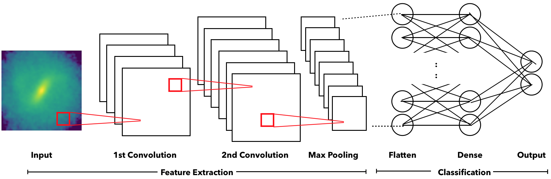
Figure 1: Schematic overview of the general architecture of a convolutional neural network. The input image is mapped into various feature maps via convolutions, followed by a pooling layer that performs local averaging and subsampling. The final layer is a list of outputs that, in our case, correspond to whether a bar is present or not.

A general schematic showing how a CNN processes an input image is shown in Figure 1. There exist many different CNN architectures in the literature (LeCun et al., 2015) that differ in the structure, type and quantity of component layers, as well as utilising different weighting and activation functions. However, memory and (computational) time limitations ultimately result in some degree of compromise between complexity and overall performance.

Our CNN architecture is based on (Bekki et al., 2019), with the goal of inputting a 50x50 density map and outputting a label to indicate whether or not a bar was detected. We used Keras for the CNN construction (Chollet et al., 2015). There are 2 convolution layers (Conv2D), a max-pooling layer (MaxPooling2D), two dropout layers (Dropout), a flatten layer (Flatten) and finally two dense layers (Dense) that are fully-connected (including the output layer). The role of the convolution layers is to extract the high- level features of the preceeding layer. This is done via the use of a kernel filter that performs a matrix operation, progressively scanning through the input layer. In our network, each Conv2D layer uses a 3x3 kernel. Our 50x50 input image is mapped into 32 separate convolved feature maps via the first Conv2D layer. These maps are then further convolved into 64 separate feature maps via the second Conv2D layer. Each of these convolutional layers can be thought of as a layer of abstraction, enabling higher-level features to be extracted.

The next major part of the architecture is the MaxPooling2D layer. In general, a pooling layer is designed to average out the convolved feature maps through downsampling. Instead of averaging, MaxPooling2D returns local maxima. This achieves two major goals: firstly, it decreases the computational complexity, while secondly the max-pooling retains the dominant features from the convolved feature map. The Flatten layer is used to vectorise the feature maps, while the Dropout layers are used to avoid over-fitting by ignoring a fraction of the preceding nodes. The final fully-connected Dense layer (before the output layer) thus combines the flattened nodes. From here on, the architecture is similar to that of a basic neural network; the weights and biases of the Dense layer nodes can be tweaked in order to associate different high-level features with the desired output category. For our CNN, we used the ReLu activation function for the convolution and dense layers, whilst the final output layer used a softmax (normalised exponential) activation with the categorical cross-entropy loss function. For training, we used the ADADELTA adaptive learning rate method, developed by Zeiler (2012). This core architecture was used for both parts of our investigation, the only crucial difference being that the CNN used to test multiple bar formation mechanisms had an extended output layer in order to account for the new labelling scheme.

2.3 Differences with existing bar detection techniques

There are several existing methods in which to both detect bars and analyse their physical characteristics; ellipse fitting of the galaxy isophotes, Fourier analysis of the (azimuthal) luminosity profile and a decomposition of the surface brightness distribution (Prieto et al., 2001). These methods involve significant pre and post-processing, and often require access to additional data such as spectroscopic flux measurements and velocity dispersion maps. Hence these methods cannot readily determine the presence of a bar from mere images alone. Another method involves directly analysing the image of a galaxy using Fourier techniques. These methods are well-known to detect the presence of stellar bars and spiral arms, as well as characterise their shape and strength (Garcia-Gómez & Athanassoula, 1991; Aguerri et al., 1998; Barberà et al., 2004; Garcia-Gómez et al., 2017).

CNNs are similar to Fourier transforms in this regard, as their core operation revolves around the detection of high-level features. Morphological classification is thus a natural application. Another difference with our CNN approach is that it avoids much of the extra image processing needed in traditional methods more suited to observational data (see (Prieto et al., 2001)). Furthermore, the CNN can be trained on images with high inclination, whereas methods similar to Garcia-Gómez et al. (2017) must perform a de-projection.

The bottleneck for CNNs lies with the training. Once trained, CNNs can quickly analyse images and output a label corresponding to what it has detected the image to be. Existing methods are tailored for real-world data, whereas our CNN is specifically designed to work with the output of our galaxy simulations. It is computationally expensive to accurately model luminosity profiles. Our CNN works with the output of dynamical N-body simulations, allowing it to be trained and tested on a larger dataset than we would otherwise have been able to compile. Our CNN-based approach to bar detection is merely tackling the problem from a different angle (i.e feature detection with CNNs) where all we are given is the image of the galaxy. It is not designed to supplant nor contest any existing method; rather it is a tool well suited to our aim of analysing many galaxy simulations in order to constrain parameters based on how many bars are detected.

3 Simulation and implementation

3.1 Structure and kinematics of the stellar disk

We consider merging of two spiral galaxies with various bulge-to- disk-ratios and baryonic mass fractions in order to investigate how stellar bars can be induced during galaxy merging. The total masses of dark matter halo, stellar disk, gas disk, and bulge of a disk galaxy are denoted as $M_{\rm h}$, $M_{\rm s}$, $M_{\rm g}$, and $M_{\rm b}$, respectively. In these preliminary works, we only show the results for models with no gas ($f_{\rm g}=M_{\rm g}/M_{\rm s}=0$) The bulge-to-disk-ratio is defined as $M_{\rm b}/M_{\rm s}$ and represented by the parameter $f_{\rm b}$. The key parameters in the present study are $M_{\rm h}$, $f_{\rm bary}$, and $f_{\rm b}$. We adopt the density distribution of the NFW halo Navarro et al. (1996), as suggested from CDM simulations, to describe the initial density profile of the dark matter halo in a disk galaxy:

$${\rho}(r)=\frac{\rho_{0}}{(r/r_{\rm s})(1+r/r_{\rm s})^{2}},$$ (1)

where $r$, $\rho_{0}$, and $r_{\rm s}$ are the spherical radius, the characteristic density of the halo, and the scale length of the halo respectively. The $c$-parameter ($c=r_{\rm vir}/r_{\rm s}$, where $r_{\rm vir}$ is the virial radius of a dark matter halo) along with $r_{\rm vir}$ are chosen appropriately for a given dark halo mass($M_{\rm dm}$) by using the $c-M_{\rm h}$ relation for $z=0$ predicted by recent cosmological simulations, e.g Neto et al. (2007).

The bulge of the disk galaxy has a size $R_{\rm b}$ and a scale-length $R_{\rm 0,b}$, and is represented by the Hernquist density profile. The bulge is assumed to have an isotropic velocity dispersion, with radial velocity dispersion given by the Jeans equation for a spherical system (Binney & Tremaine, 2008). The bulge-to-disk ratio ($f_{\rm b}=M_{\rm b}/M_{\rm d}$) of the disk galaxy is a free parameter ranging from 0 (pure disk galaxy) to 1. Our ‘MW-type’ models are those with $f_{\rm b}=0.17$ and $R_{\rm b}=0.2R_{\rm s}$, where $R_{\rm s}$ is the stellar disk size of a galaxy. We adopt the mass-size scaling relation of $R_{\rm b}=C_{\rm b}M_{\rm b}^{0.5}$ for bulges such that we can determine $R_{\rm b}$ for a given $M_{\rm b}$. The value of $C_{\rm b}$ is determined in order for $R_{\rm b}$ to be 3.5 kpc for $M_{\rm b}=10^{10}{\rm M}_{\odot}$ (this corresponds to the mass and size of the MW’s bulge).

The radial ($R$) and vertical ($Z$) density profiles of the stellar disk are assumed to be proportional to $\exp(-R/R_{0})$ with scale length $R_{0}=0.2R_{\rm s}$ and to ${\rm sech}^{2}(Z/Z_{0})$ with scale length $Z_{0}=0.04R_{\rm s}$, respectively. In the present model for the MW-type, the exponential disk has $R_{\rm s}=17.5$ kpc. In addition to the rotational velocity caused by the gravitational field of disk, bulge, and dark halo components, the initial radial and azimuthal velocity dispersions are assigned to the disc component according to the epicyclic theory (Toomre, 1964) with Toomre’s parameter set to $Q$ = 1.5. The vertical velocity dispersion at a given radius is set to be 0.5 times as large as the radial velocity dispersion at that point.

The total numbers of particles in a fiducial model with $f_{\\ rmb}=0.167$ is 216700, though for other models it depends on $f_{\rm b}$. The mass resolution for each of the models in the present study is $1.2\times 10^{6}{\rm M}_{\odot}$. The gravitational softening length for each component is determined by the number of particles used for each component, as well as by the size of the distribution (e.g., $R_{\rm s}$ and $r_{\rm vir}$). It is set to be 320 pc, which is much finer than $1-2$ kpc spatial resolutions used for the image analysis in the present study. These spatial and mass resolutions are not particularly high; this is predominantly because we have to run a large number of models within a limited amount of GPU computing time allocated for this project. We believe that the adopted resolutions and subsequent galaxy images are sufficient for use with the CNNs. A summary of our simulation parameters and features is provided in Table 1.

Table 1: Description of the basic parameter values for the MW-type disk model.

Physical properties	Parameter values
Total halo mass (galaxy)	$M_{\rm dm}=1.0\times 10^{12}{\rm M}_{\odot}$
DM structure (galaxy)	NFW profile
Galaxy virial radius (galaxy)	$R_{\rm vir}=245$ kpc
$c$ parameter of galaxy halo	$c=10$
Stellar disk mass	$M_{\rm s}=6.0\times 10^{10}{\rm M}_{\odot}$
Stellar disk size	$R_{\rm s}=17.5$ kpc
Disk scale length	$R_{0}=3.5$ kpc
Gas fraction in a disk	$f_{\rm g}=0$
Bulge mass	$M_{\rm b}=10^{10}{\rm M}_{\odot}$
Bulge size	$R_{\rm b}=3.5$ kpc
Mass resolution	$1.2\times 10^{6}{\rm M}_{\odot}$
Size resolution	320 pc
Spatial resolution for image analysis	1-2 kpc
Star formation	Not included
Chemical evolution	Not included
Dust evolution	Not included

3.2 Orbital configurations for galaxy merging

In all of the merger simulations with different mass-ratios of two disks ($m_{2}$), the orbit of the two disks is set to be initially in the xy plane. The initial distance between the center of mass of the two disks, the pericenter distance, and the circular velocity factor ($f_{\rm v}$) for the companion galaxy are set to be $8R_{\rm s}$, $2R_{\rm s}$, and 0.5 respectively for all models. For this study, we have set the velocity of the two disk such that all orbits are prograde and initially confined to the xy plane. We define $f_{\rm v}$ as the ratio of the total 3D velocity of the companion galaxy (with respect to the primary galaxy) to the circular velocity at the distance of the companion from the center of the primary galaxy. The azimuthal angle $\phi$ is measured from the x-axis to the projection of the angular momentum vector of the disk onto the x-y plane. This is set to be 0 for both disk galaxies, as it is not an important parameter in the present study. The time when the progenitor disks merge completely and reach the dynamical equilibrium is typically less than 12.0 in our units for most of models.

3.3 Definition of mass ratio and spin angles

We define the mass ratio $m_{2}$ as the ratio of the mass of the companion galaxy to that of the parent. We refer to a minor merger as a merger with $m_{2}\approx 0.1$, and a major merger as that with $m_{2}\approx 1$. We also refer to intermediate mass mergers as those with $m_{2}$ between 0.1 and 1. The spin of each galaxy is specified by two angles, $\theta_{i}$, where the subscript i is used to identify each galaxy ($\theta_{1}$ for the primary galaxy, $\theta_{2}$ for the companion). The spin angles $\theta_{i}$ are defined as the angle between the z-axis and the vector of the angular momentum of the disk. In our present study, we vary these angles between $-180$ and $180$ degrees.

3.4 Simulation output and training data

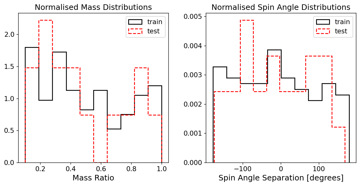
Figure 2: Normalised histograms showing the distributions of mass ratios (left) and $\theta_{1}-\theta_{2}$ (right) for the training and testing sets.

The raw density output from our simulations comprised a list of local density values ordered by pixel for each of the 200 different viewing angle orientations, with separate files for each model and time-step. We derive 2D density maps of our simulated galaxies for $R\leq R_{\rm s}$. We first divide the stellar disk ($R\leq R_{\rm s}$) of the galaxy into a $50\times 50$ grid mesh and estimate the mean stellar mass density at each mesh point as follows:

$$\Sigma_{i,j,0}=\frac{1}{{\Delta R_{i,j}}^{2}}\sum_{k=1}^{N_{\it i,j}}m_{k},$$ (2)

where $\Delta R_{i,j}$, $N_{i,j}$, and $m_{k}$ are the mesh size at the mesh point ($i$, $j$), the total number of stellar particles in the mesh, and the mass of a stellar particle, respectively. These values were normalised to obtain the normalised density maps. The mesh size is set to $0.04R_{\rm s}$, which roughly corresponds to 0.7 kpc for an MW-type disk galaxy.

To create the training data for our CNN, the raw density data was stitched together to create 50x50 images (corresponding to the normalised density maps). Thus the input layer to our neural network consisted of a linear array of 2500 pixel values corresponding to the 50x50 density maps. This is how the individual images were tested with the neural network. For each individual galaxy model, we obtained a total of 200 images that differed in orientation and inclination. This is to ensure that the training set includes images of bars with different projections and orientations, and to mirror real life data.

These density maps, totalling 29,400 total images, were combined to create the training set for the CNN. Each of these training images were manually assigned a label (corresponding to a bar or no-bar) through visual inspection in order to create the input-output pairs with which to train the CNN. The visual classification was conducted by both authors, restricted to only the face-on images for each model. On average, 1 in 20 images were classified different by each observer. These were overwhelmingly galaxies with oblate bulges, where the distinction between a bar and a bulge is not so objectively clear. As a result, we estimate that the overall labelling of the training set is 95% accurate (i.e there is an overall uncertainty of around 5%). A key aspect of any training set is that should be a roughly equal number of samples for each of the classification categories, otherwise there is a bias towards the category with the greater number of samples. In our case, that means ensuring the number of barred and non-barred galaxy samples are about the same. Many of our simulations were thus manually checked to see whether or not a bar had been formed. The training set was split into separate training and validation sets such that 80% of the samples were used to train, with the remaining 20% used for validation. The validation data was randomly partitioned from the main sample set. Figure 2 shows the distribution of mass ratio and angular separation ($\theta_{1}-\theta_{2}$) for the training and test sets. Ideally these should be uniform, although there is a slight bias towards samples with lower mass ratios samples.

We define the prevalence of bar formation in a given model as the fraction of the 200 images that returned a label of “bar” when tested with the CNN. We performed these tests for density outputs with different values of mass-ratio $m_{2}$ and spin- angles $\theta_{1}$ and $\theta_{2}$, for different galaxy models with different bulge-to-disk ratios and dark matter contents. A full description of the exact parameters used for each model is provided in Table 2.

Table 2: Dark matter, stellar, bulge components and bulge-to-disk ratios for each of our six models

Model	Dark Matter	Stellar Mass	Bulge Mass	Bulge-to-disk
	$10^{12}M_{\odot}$	$10^{10}M_{\odot}$	$10^{10}M_{\odot}$	ratio
m1	1	6	1	0.167
m2	1	3	0.5	0.167
m3	1	1.8	0.3	0.167
m4	1	6	3	0.5
m5	1	6	6	1
m6	1	6	0	0

3.5 Training the network

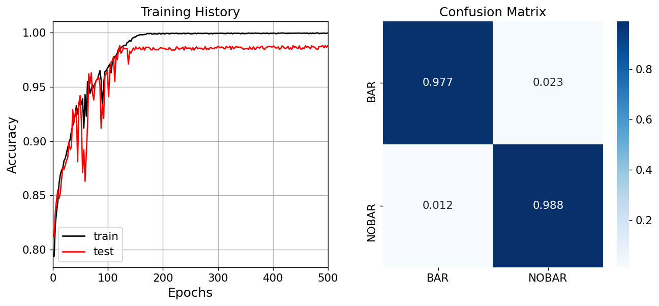
Figure 3: Plot of the training and testing (validation) accuracies against training time (left), as well as the confusion matrix (right) for the main CNN

The CNN was coded using Keras (Chollet et al., 2015), a high- level deep learning application programming interface (API), running on TensorFlow, a machine learning framework. Training was conducted on the ICRAR’s Pleiades cluster, making use of a Nvidia GTX1080. Here all 29,400 images were used to train the CNN, with training conducted in stages up to a combined total 1000 epochs. The training and validation accuracies, along with a confusion matrix, are presented in Figure 3.

The validation accuracy converged to between 98% and 99% within around 200 epochs, after which there was no further increase. Given that this is well above what would be expected due to the 5% uncertainty inherent in the training set, it is likely that there is some degree of overfitting. The batch-size was set to 200 images, given that this corresponds to a single galaxy model. Modifying the batch size did not appreciably impact the final accuracy. Training for our secondary, multiple-bar classification CNN was also conducted on Pleiades, however this used a much smaller subset of 4800 images.

To achieve our primary goal of constraining bar formation in galaxy merging, we conducted simulations with varying mass-ratios and spin angles $\theta_{1},\theta_{2}$ for both disk-dominated and bulge- dominated initial disks. The output from these simulations were then tested with the CNN. Since each simulation output has 200 associated density maps (each oriented differently with respect to the viewing axis), we define the prevalence of bar formation as the fraction of these 200 images that are classified as a bar by the CNN. That is, we define the bar fraction as:

$$f_{\text{bar}}=N_{\text{bar}}/N$$ (3)

where $N_{\text{bar}}$ are the number of images detected as showing a bar, and $N$ is the total number of images. We also refer to this as the bar probability, with the terms used interchangeably depending on the context. We ran several disk-dominated and bulge- dominated models, and tested the outputted data with our fully- trained CNN to determine the prevalence of bar formation as functions of mass ratio $m_{2}$ and spin angles $\theta_{1},\theta_{2}$.

Our secondary goal of using a CNN to distinguish between different bar formation mechanisms used a new CNN with the same core architecture with two key differences: it was trained on a different set of simulated data, and utilised a different labelling schema (4 categories instead of 2).

4 Results

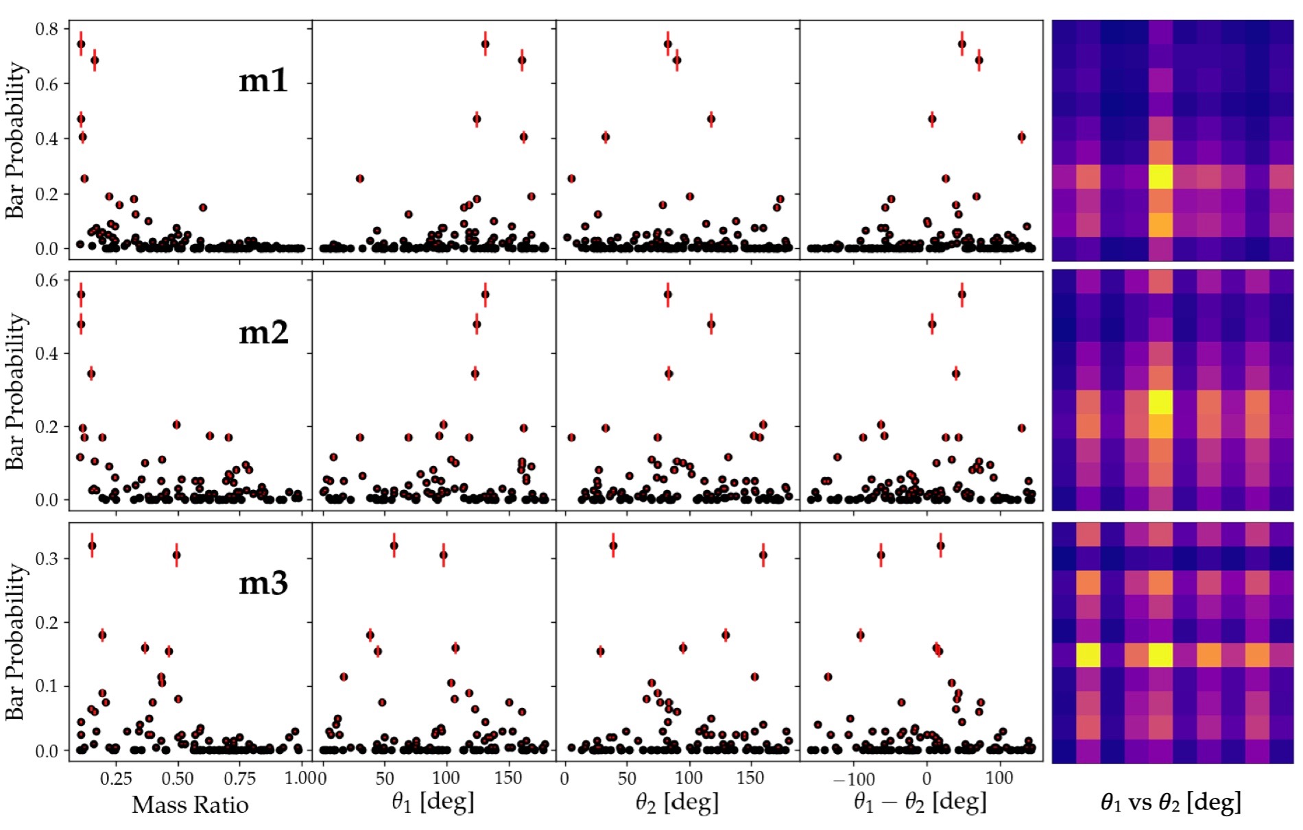
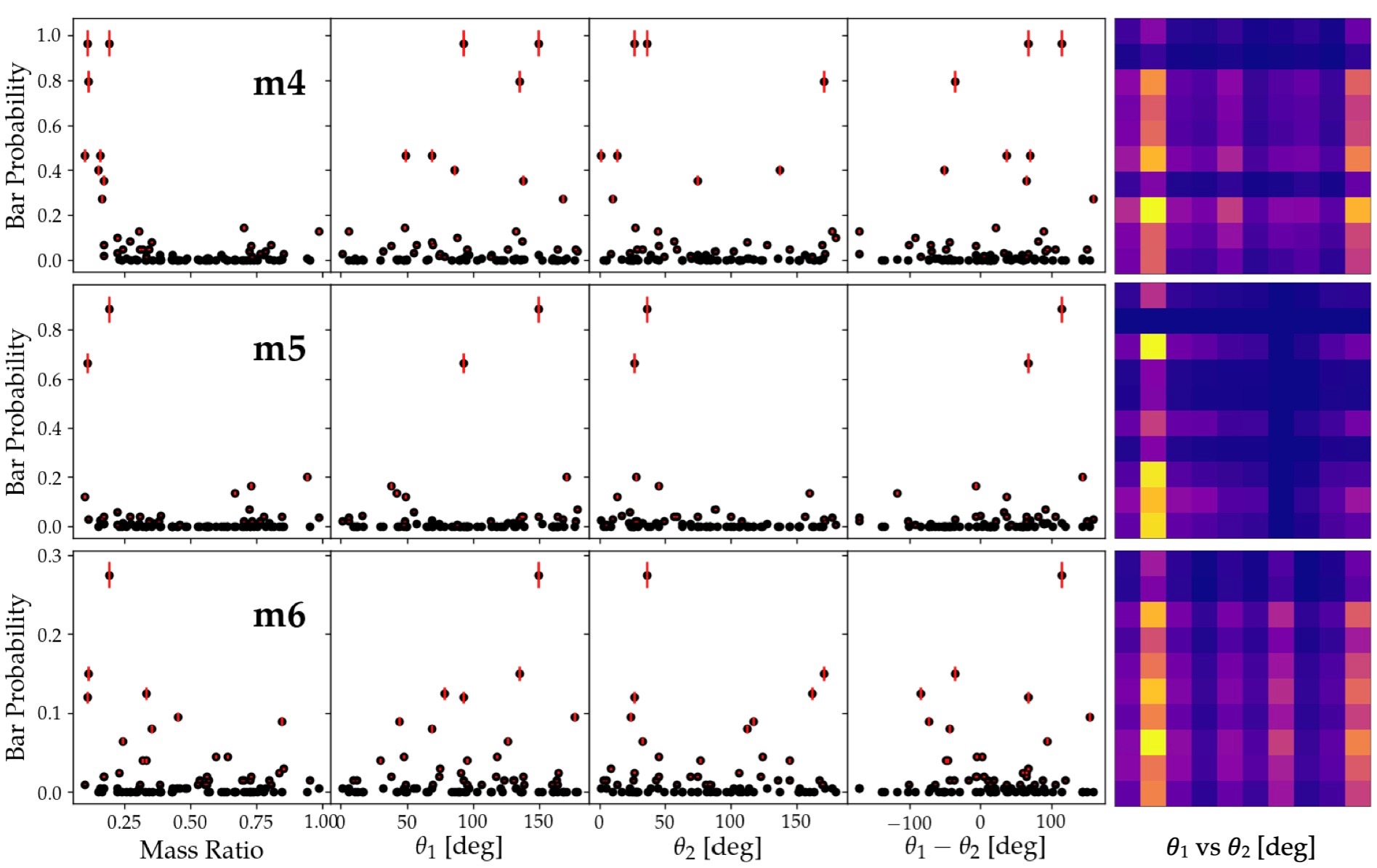
Figure 4: Incidence of bar formation, expressed as the bar fraction $f_{\text{bar}}$ or bar probability, as a function of mass ratio $m_{2}$, the difference in spin angle $\theta_{1},\theta_{2}$, and as a function of $\theta_{1}$ vs. $\theta_{2}$ where $\theta_{1}$ is on the vertical axis. Lighter shades in the normalised density map of $\theta_{1}$ vs $\theta_{2}$ indicate a higher relative probability of bar detection. Error bars indicate one standard error $\sigma$.

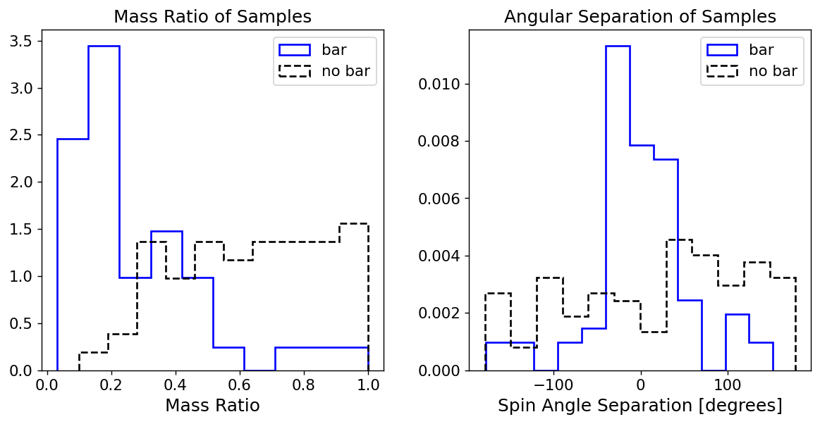
Figure 5: Normalised histograms of all samples classified as either bar (blue) or no-bar (black, dotted) by our main CNN, for different mass ratios (left) and spin angle separation (right).

Table 3: Total bar fractions for the variable mass ratio $m_{2}=0.1$ to 1.0 and fixed mass ratios $m_{2}=0.1$ and $m_{2}=1.0$, for each of our six galaxy models.

Model	Bar fraction	Bar fraction	Bar fraction
	$m_{2}=0.1$ to $1.0$	$m_{2}=0.1$	$m_{2}=1.0$
m1	0.075 $\pm$ 0.0037	0.082 $\pm$ 0.0041	0.013 $\pm$ 0.00065
m2	0.064 $\pm$ 0.0032	0.073 $\pm$ 0.0036	0.029 $\pm$ 0.0015
m3	0.048 $\pm$ 0.0024	0.051 $\pm$ 0.0026	0.03 $\pm$ 0.0015
m4	0.12 $\pm$ 0.006	0.11 $\pm$ 0.0055	0.038 $\pm$ 0.0019
m5	0.089 $\pm$ 0.0044	0.091 $\pm$ 0.0045	0.057 $\pm$ 0.00285
m6	0.037 $\pm$ 0.0019	0.037 $\pm$ 0.0019	0.036 $\pm$ 0.0018

4.1 Mass ratio

To investigate the effects of mass ratio, we ran several hundred simulations for each of the six galaxy models in Table 2 for a variable mass ratio ($m_{2}$ between 0.1 and 1.0) as well as for the fixed mass ratios $m_{2}=0.1$ (corresponding to minor merging) and $m_{2}=1.0$ (corresponding to major merging). Each of the simulations were conducted with random spin angles such that $0\leq\theta_{i}\leq 180$ degrees for $i=1,2$. These models are completely separate from those used to train the CNN. Instead, these models were classified by the fully-trained CNN.

Table 3 shows the detected bar fractions (i.e as defined in Equation 3) for each of these three mass cases for our six galaxy simulation models (refer to Table 2 for their physical parameters). On average, the CNN detected more bars present in the aftermath of minor merging ($m_{2}$ on the order of $0.1$) as opposed to major merging ($m_{2}\sim 1.0$). Figure 4 gives a visualisation of the bar probability as functions of the parameters $m_{2},\theta_{1},\theta_{2},\theta_{1}-\theta_{2}$ and finally as a normalised probability density map corresponding to $\theta_{1}$ vs. $\theta_{2}$. Again we see a clear inverse relationship with mass ratio; lower mass ratios are more conducive to bar formation.

Figure 5 gives a more compact visualisation of the overall CNN classifications, showing the normalised histograms of all samples classified as bar or no-bar with respect to mass ratio and spin angles. As seen in Figure 4, of those samples classified as bars, they generally have lower mass ratios and lower angular separation. Conversely, samples classified as no-bar tend to have mass ratios between 0.3 and 1.0, and are uniform with regards to angular separation. This latter result suggests that mass ratio is a more influential factor in the bar formation process.

It is important to stress that the results in Figures 4 were obtained by running limited sets of random parameter combinations. Due to time limitations, it was impossible to cover all combinations of $m_{2},\theta_{1}$ and $\theta_{2}$, but there are enough data points to qualitatively infer trends and pinpoint certain parameter ranges that are more conducive to bar formation than others.

In Figure 4, we see both reciprocal relationships (such as the m1 model) and a relationship with two distinct peaks (the m3 model). This suggests that intermediate-mass mergers may be just as efficient as minor mergers at producing bars for certain galaxy models (in the case of m3, a galaxy model with a smaller stellar mass). For all models, major merging is far less conducive to bar formation compared to minor merging. Further simulations with a wider range of model parameters are required to definitively examine the mathematical nature of this relationship.

4.2 Spin angles

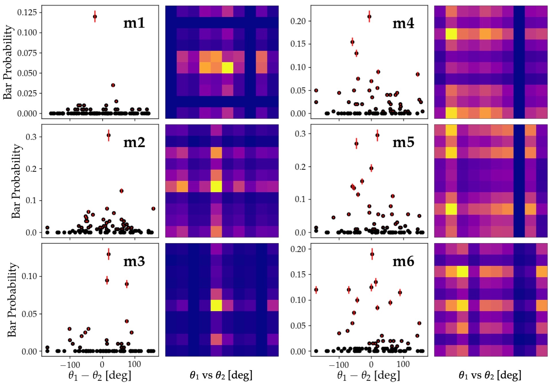
Figure 6: The incidence of bar formation, expressed as the fraction of total images that were identified as bar for a given model, as a function of the difference in spin angles $\theta_{1}-\theta_{2}$ and as a function of spin angles $\theta_{1}$ vs.$\theta_{2}$ for major mergers at a fixed mass ratio of 1.0.

The m1, m2 and m3 models appear to be more strongly constrained by $\theta_{1}$, while there is a dominant $\theta_{2}$ constraint for the m4, m5 and m6 models. Given the significant scatter in the overall spin angles, more simulations are needed to conclusively determine any specific constraints on either angle. Since the exchange of angular momentum is an important factor of bar formation, it is better to focus on the difference in the spin angles, $\theta_{1}-\theta_{2}$ (i.e how closely aligned the disks are). We find that, for the m1, m2 and m3 models, more bars were detected for more closely aligned $\theta_{1}$ and $\theta_{2}$ (i.e $|\theta_{1}-\theta_{2}|\approx 0$) compared to mergers with wildly different spin angles. However, such a trend is not observed for the m4, m5 and m6 models in the variable-mass case.

In order to analyse these spin angle constraints independently of mass ratios, we ran several models for all 6 of our galaxy merger models with a fixed mass ratio of 1.0 (Figure 6), corresponding to major mergers. We previously established that fewer bars were detected in major merging; hence testing on major mergers yields a stronger constraint on the spin angles. Again, we find that models in which $\theta_{1}$ and $\theta_{2}$ are more closely aligned resulted in the detection of more bars. In each case, the parameter with the highest fraction of bar detection is located very close to $\theta_{1}-\theta_{2}=0$. This is also true for the m4, m5 and m6 models. Importantly, these results were consistent across our various models despite their differences in bulge-to-disk ratios and dark matter contents.

5 Discussion

To verify these constraints, we first identified several key cases that involved contrasting two simulation models. The most important of these test cases is to compare a major merger with a minor merger. We did this for the small-bulge m1 disk model (Figure 7) as well the large-bulge m4 model with a bulge- to-disk ratio of 0.5 (Figure 9). We decided to use the m1 model instead of the bulge-less m6 model, and the m4 model instead of the 1:1 bulge-to-disk m5 model, in order to keep in line with more realistic MW-type galaxies.

Since our models in Figures 4 and 6 found that mergers with low angular separation were more conducive to bar formation, we also analysed a major merger for equal spin angles $\theta_{1}=\theta_{2}=0$. The latter of these cases is highly unrealistic given how statistically unlikely it is for two prograde galaxies to merge with the same orientation. We also compared a simulation of the m4 model in the isolated and minor merger case.

5.1 The bar formation process

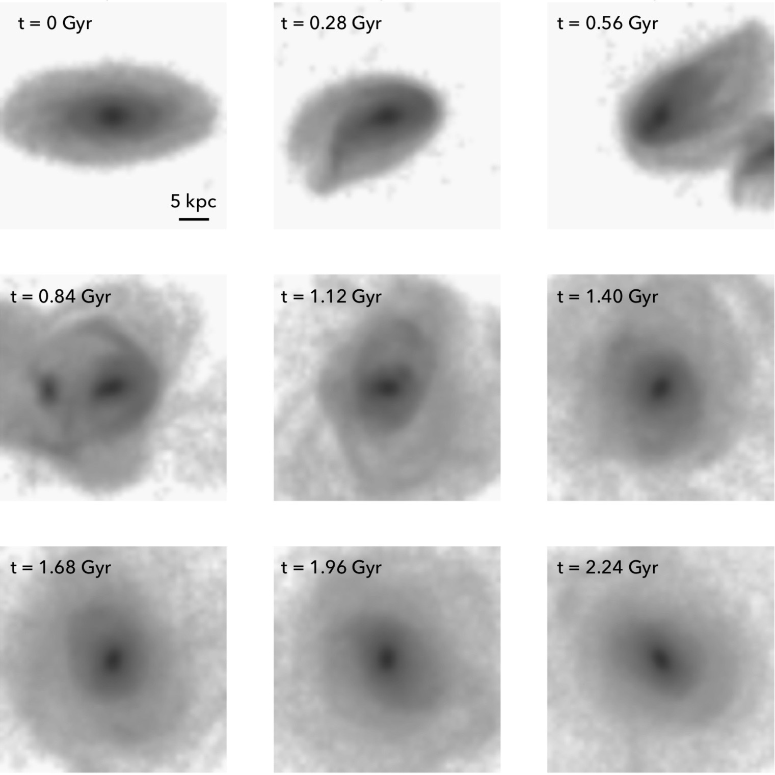
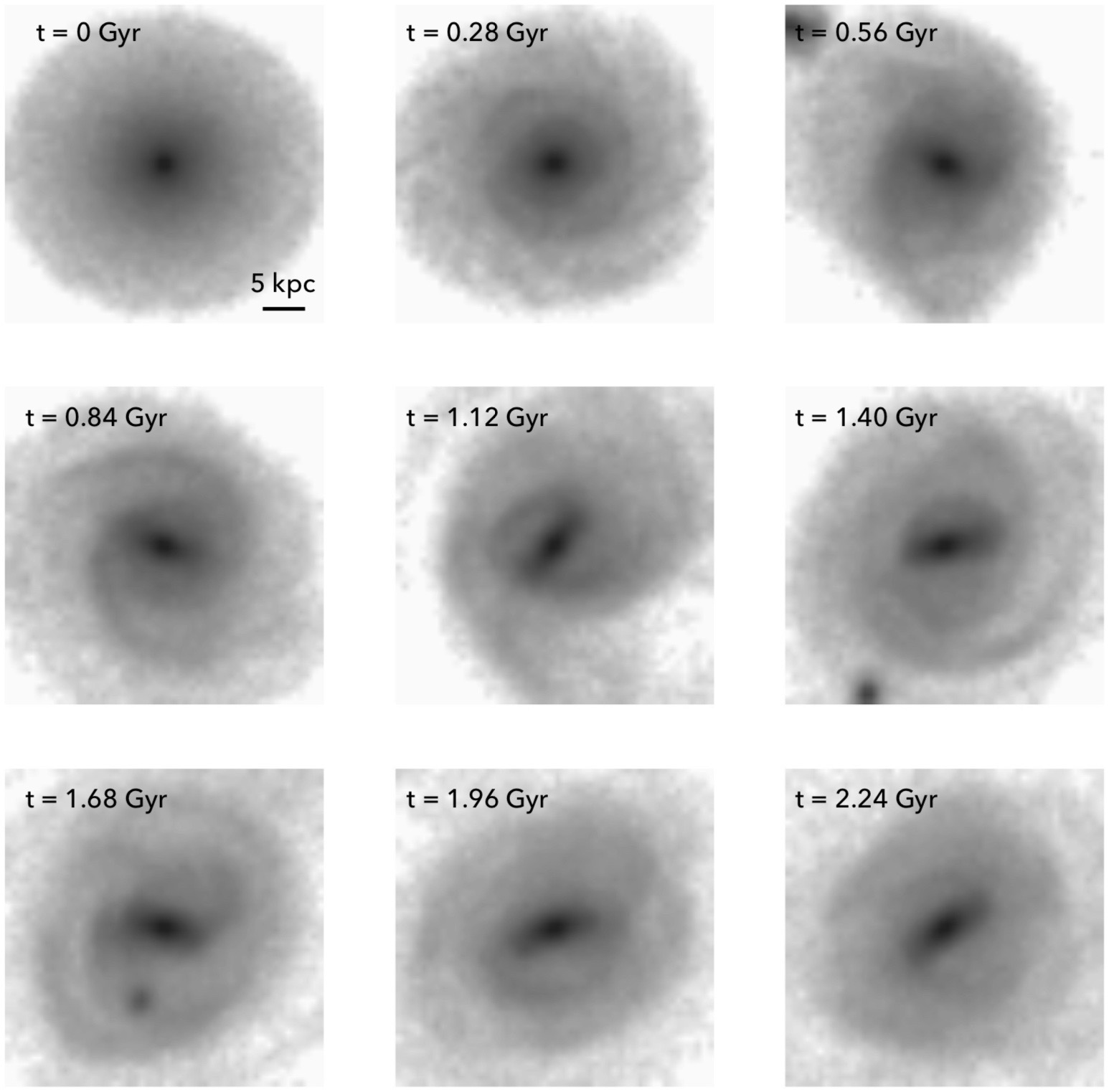
Figure 7: Time evolution of the 2D normalised mass density distribution ($x$-$y$ plane projection) for a major merger with mass ratio $m_{2}=1.0$ (top) and minor merger with mass ratio $m_{2}=0.1$ (bottom) for the small-bulge m1 model. Each frame measures 35 kpc by 35 kpc (these dimensions are used throughout) and each timestep is 240 Myr.

It is clear from Figure 7 that a stellar bar is readily formed in the minor merger case, while no bar is produced in the major merger. Importantly, the major and minor merger cases are distinguished by the timescale of the merger. In the major merger case, the galaxies merge destructively between 840 Myr and 1.12 Gyr, while the minor merger completes between 1.68 Gyr and 1.96 Gyr (some 800 Myr later). Our simulation results in Figure 4 have shown that minor merging is more conducive to bar formation. This is important considering the well-studied effects of minor merging in the overall evolution of galaxies (Reichard et al., 2008). Simulations have also shown the vast majority of all mergers in the Universe to be minor mergers (Lotz et al., 2010). It is important, however, to keep in mind the low overall bar detections in Table 3; bar formation in galaxy merging is rare.

In most cases where a bar is detected in the aftermath of the merger event, the bar is first formed due to tidal interaction with the approaching galaxy, after which it then survives the merger process. In the case of major merging, the merger is destructive. Conversely, minor merging is constructive. This is sensible given the difference in gravitational effects. Smaller companions tend to slowly spiral into their parent (helping to induce a tidal bar), and by the time the merger is complete they are usually sufficiently stripped of mass so as to not warp or disturb the parent disk. Equal mass mergers are more destructive due to the quick head-on collision (such as what we see in Figure 7) that severely warps the stellar disk.

It is this latter notion of whether a bar survives or is destroyed that is they key motivation behind finding constraints for our simulation parameters. These constraints will help guide further investigation into the exact mechanisms with which bars can survive a galaxy merger unscathed. It is important to note that there are two mechanisms at play here; the initial pre-merger tidal interactions, and the actual merger itself. Previous studies, e.g (Peirani et al., 2009; Di Matteo et al., 2010), have shown that bars can form due to the tidal interactions before a merger, however they did not consider what happens to the bar during the merger itself. To better illustrate this dual-nature, Figure 8 shows a major merger with $\theta_{1}=\theta_{2}=0$ degrees.

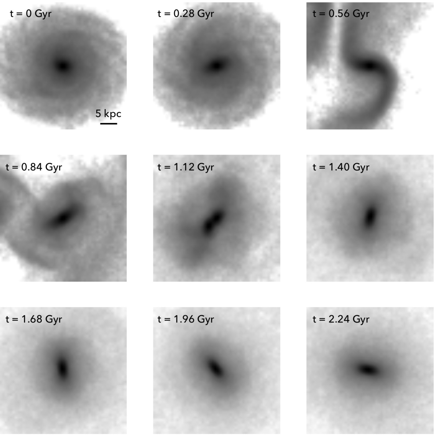
Figure 8: Time evolution of the 2D normalised mass density distributions for our simulations of a major merger for $\theta_{1},\theta_{2}=0$, demonstrating the formation of a bar in a major merger with $\theta_{1}=\theta_{2}=0$ degrees. Frame dimensions are as in Figure 7

First and foremost, Figure 8 shows bar formation in the major merger case. So although the results of Figure 4 show that minor merging is much more promising, we have demonstrated that bar formation is still possible for major mergers. The spin angles (i.e the orientation of the galaxies) are also key to whether or not a bar is produced. In Figure 8, we see that a bar is induced at around 0.56 Gyr. The actual merger takes place between 0.84 and 1.12 Gyr. However, the snapshot at 1.12 Gyr shows the bar has buckled into two loosely connected bulges (likely due to the force of the merger), but by 1.40 Gyr the stellar bar has reformed and continues to exist for the rest of the simulation timescale. This is strong evidence for the role of spin angles in the formation and survival of stellar bars in merging. So while it is possible for bars to be induced prior to the merger due to tidal interactions, regardless of orientation (as tidal interactions are gravitational in nature), orientation is key to whether a bar can be reformed in the aftermath of a galaxy merger. It is this latter mechanism that we wish to highlight in this current study.

Angular momentum is a key factor in galaxy merging (Athanassoula, 2005; Pedrosa & Tissera, 2015). The results of Figures 6 and Figure 8 show that major mergers with more closely aligned orientations (i.e $\theta_{1}-\theta_{2}|=0$) have higher bar detection rates. This is likely due to a more favourable transfer of angular momentum that, as Figure 8 shows, is sufficient to regenerate the stellar bar.

Thus we have shown that there are two distinct phases that govern the overall bar formation process in galaxy merging; (1) pre-merger tidal interactions, and (2) reformation of the bar during and/or after the merger. Our results have shown that the minor merging of two galaxies with near-identical spin angles is most conducive to bar formation in the aftermath of a merger. This highlights the importance of angular momentum transfers, and also the role of gravitational forces given the sharp decline in bar detections as the mass ratio increases. We expect that the second phase is more dominant in major merging due to the destructive nature of the merger whereby strong gravitational forces greatly perturb the stellar disk.

5.2 Effect of stellar bulges

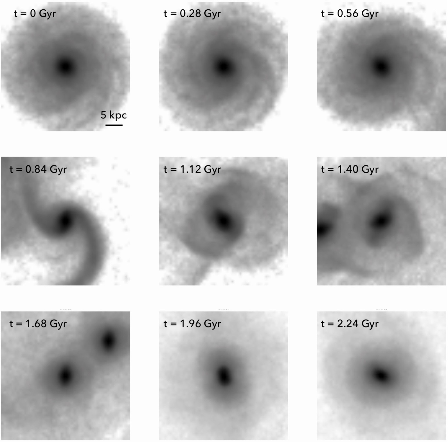
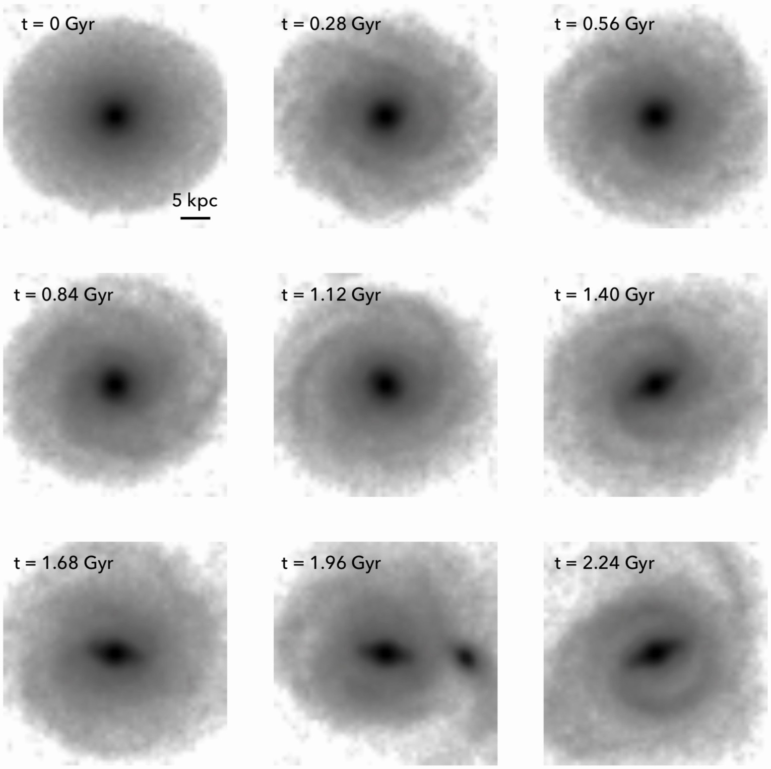
Figure 9: Time evolution of our simulations of a major merger with mass ratio $m_{2}=1.0$ (top) and a minor merger with mass ratio $m_{1}=0.1$ for a model with a bulge-to-disk ratio of 0.5 (bottom).

The bar fractions in Table 3 are lower for models with smaller bulges. This is somewhat counter-intuitive given that bulges tend to suppress bar formation in isolation. This suggests that a bulges may play a more important role in galaxy merging. To visualise whether stellar bulges have a meaningful impact on bar formation, we ran a test simulation with the m4 model (bulge-to- disk ratio of 0.5) for both a major and minor merger (see Figure 9). As anticipated (based on the results of Figure 4 and the bar fractions in Table 3), major merging is destructive while minor merging is constructive. A key physical observation is that the addition of a sizeable stellar bulge has increased the time taken for a bar to be induced. In the minor merging case, a bar is only induced after around 1.68 to 1.96 Gyr (considerably more time than in Figure 7). This supports the well-known dynamical role that stellar bulges play in stabilising disk instabilities (Kataria & Das, 2017) and hence inhibiting bar growth (Sellwood & Wilkinson, 1993).

5.3 Comparison to the isolated case

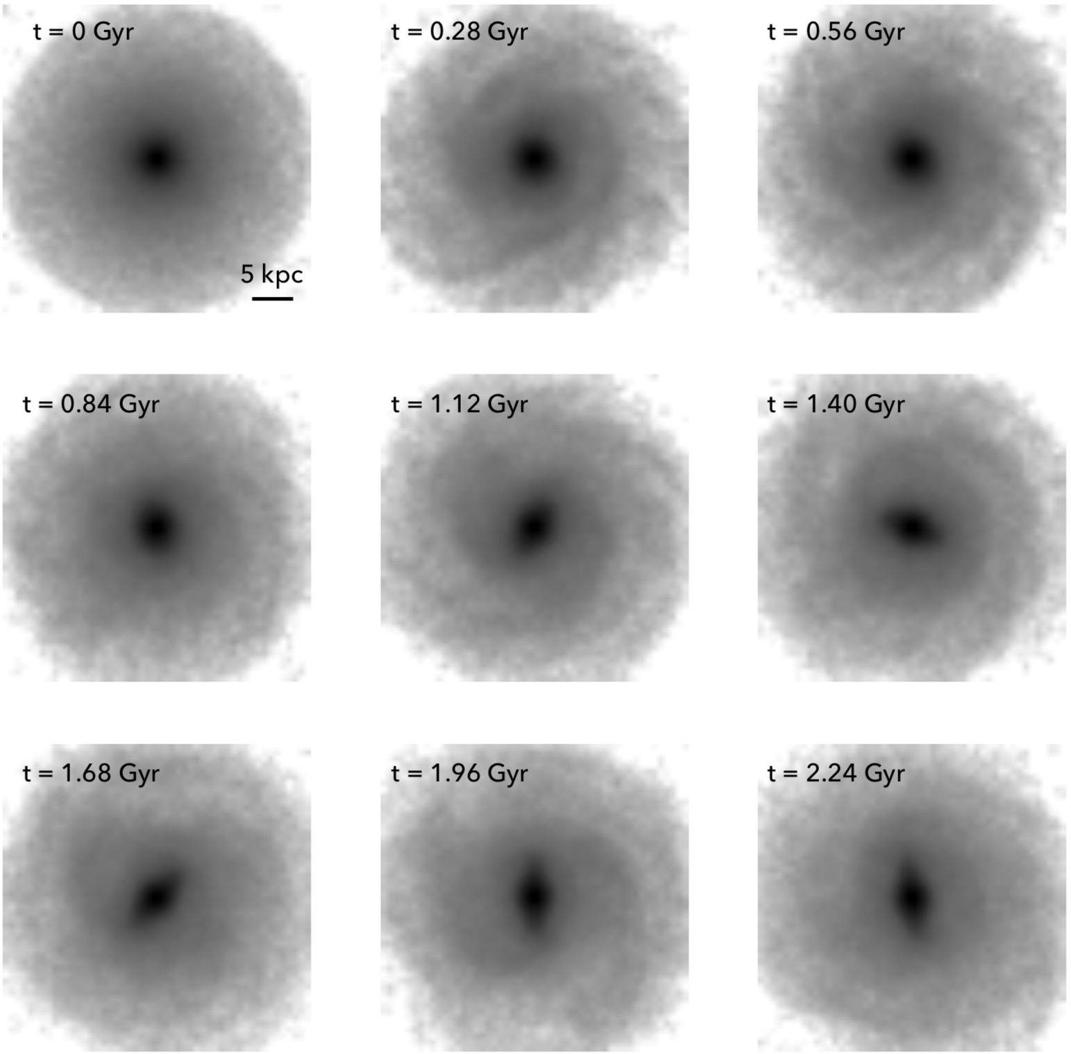
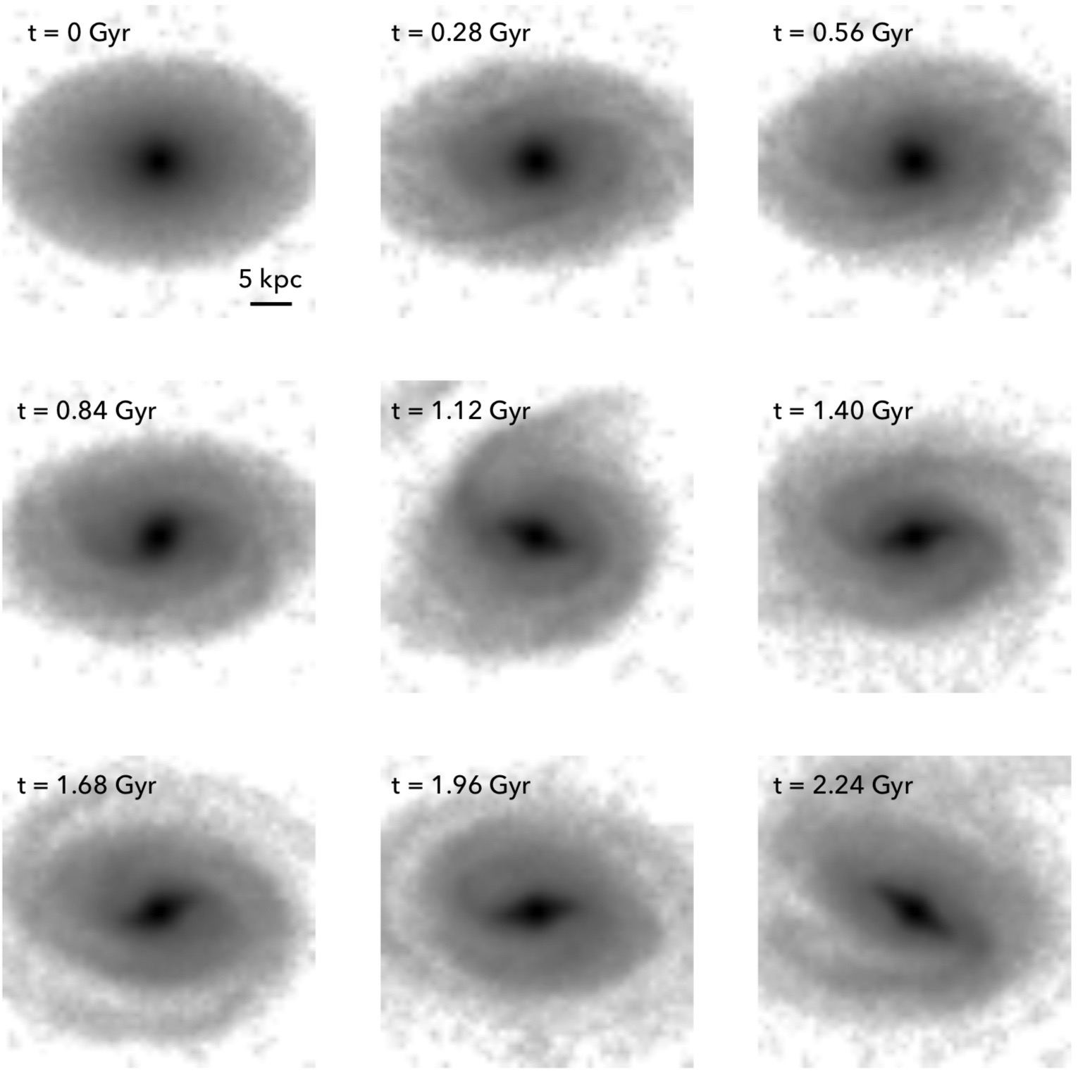
Figure 10: Time evolution of our simulations of a galaxy with a bulge-to-disk ratio of 0.5 in the isolated case (left) and merger case (right).

To better understand the role of minor merging in bar formation, we ran a simulation of the m4 galaxy model in both the isolated case and for a minor merger with mass ratio $m_{2}=0.1$ (see Figure 10). The idea is that the bulge should suppress bar formation, yet in the minor merging case of Figure 10, we see that bar is induced as early as 1.12 Gyr, while there is only evidence of a weak bar in the isolated case from roughly 1.96 Gyr onwards. The bar formed in the minor merger is more well defined and is also accompanied by spiral arms.

That minor merging can induce bars in bulge-dominant disks is particularly important since it thought that bulges can stabilise disk instabilities (Binney & Tremaine, 2008), particularly in isolation. Kataria & Das (2017) investigated upper limits on bulge-to-disk ratios for bar formation in isolation, finding that massive bulges stabilise the disk by cutting off angular momentum exchange between the disk and halo.

Lotz et al. (2010) investigated the role of mass ratios in galaxy morphology with cosmological simulation, and notes that the vast majority of galaxy mergers will be minor mergers rather than equal-mass major merging. In terms of morphological evolution, minor merging can lead to morphological distortion (Reichard et al., 2008) that ultimately affects galaxy properties (Darg et al., 2010). Minor merging is a crucial process in the formation and evolution of galaxies. We have found that mass ratio indeed plays a key role in bar formation, confirming the importance of mass ratio when studying the processes that govern galaxy merger.

5.4 Pattern speeds

One important factor to ensure the accuracy of the classifications is to determine whether the bars as seen in Figures 7, 9 and 10 are actually real bars, or instead just elongated bulges. One such method is to analyse the pattern speed $\Omega_{b}$, i.e the rate (or frequency) with which the bar rotates. The pattern speed is a very important parameter when it comes to the dynamics of barred galaxies (Sellwood & Wilkinson, 1993; Sellwood & Sparke, 1988; Athanassoula, 2005). This is since rotation is a key physical feature of bars (Sellwood & Wilkinson, 1993) that distinguishes them from elongated bulges or other irregular morphological features. There are many well established methods to analyse pattern speeds (Gerssen et al., 2003; Aguerri et al., 2015; Wu et al., 2018b) including the classic kinematic-based approach of Tremaine & Weinberg (1984) (also known as the TW method). The TW method is heavily reliant on additional data such as line-of-sight velocity maps and is more suited to observational data (see (Aguerri et al., 2015)).

6 Classifying bar formation mechanisms

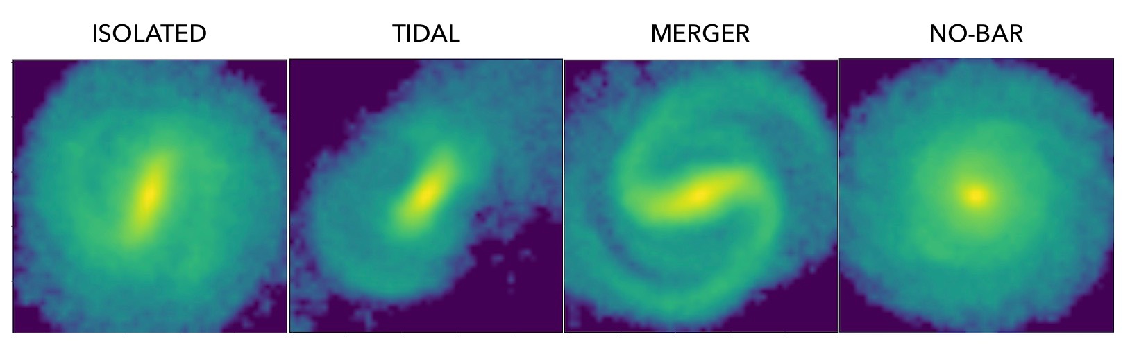
Figure 11: Images in each of the four different morphological categories considered for our secondary, bar-type CNN

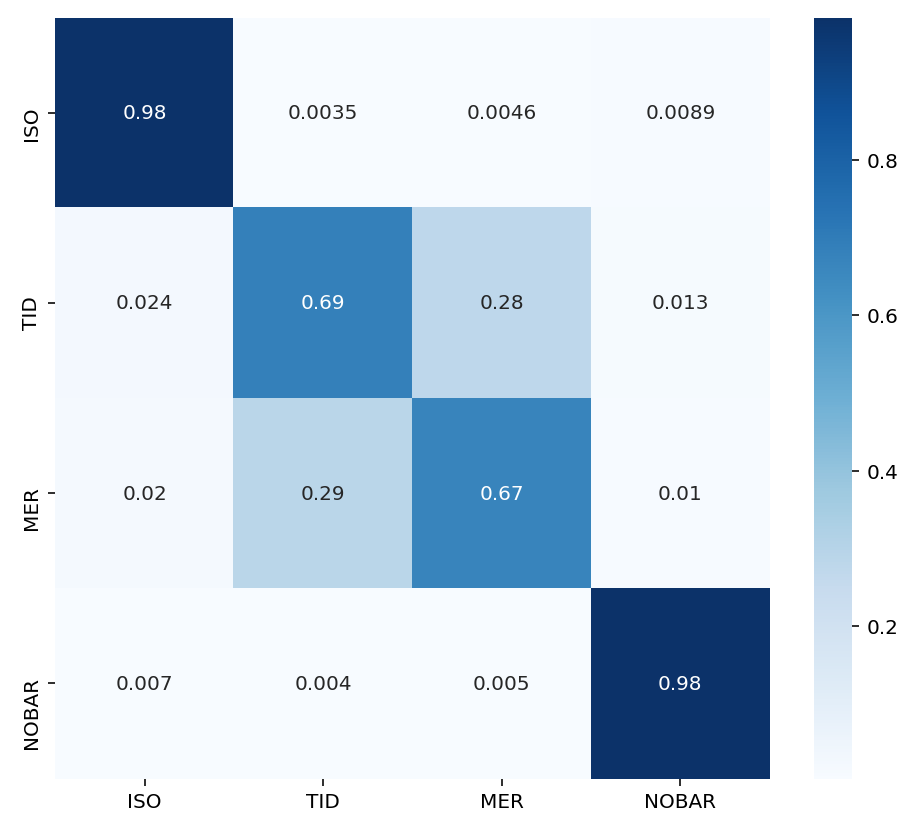
Figure 12: The confusion matrix of classification accuracies for our CNN. Here the columns represent the actual category and the rows represent the predicted category.

In this section, we discuss our secondary aim of classifying an image of a barred galaxy according to the mechanism with which it was formed. As this is a separate CNN from our main CNN, we will refer to it as the “bar-type” CNN. Figure 11 illustrates the rationale for this aim. It shows images of galaxies from our simulations in the isolated, tidal and minor merger cases, as well as an image with no bar. Just as the human eye can discern between these four cases, we wish to determine whether a CNN can do the same. For this step, we use the same CNN architecture used for our main analysis, albeit instead of 2 nodes in the output layer there are now 4 (corresponding to the 4 categories). This new network was trained with a much smaller training set of 4800 images obtained from running the m1, m2 and m3 models for the isolated, tidal and merger case (with images that showed no bar formation added to the “no- bar” category). This smaller set was visually classified up to an accuracy of 100% with both observers agreeing on all classifications, however it is likely a larger set would be subject to more uncertainty. We randomly partitioned this training set such that 80% of the samples were used the train the network, with the remaining 20% used for validation purposes. The network was trained up to maximum total accuracy over 300 epochs with the same internal architecture as the main CNN albeit it with four output nodes instead of two.

One way to determine how accurate the CNN is at distinguishing between multiple categories is by looking at the confusion matrix (a.k.a error matrix). The confusion matrix lists the actual categories and predicted categories of a set of samples. Assuming an 100% accurate network, the confusion matrix should be a diagonal matrix.

As can be seen from the confusion matrix of our bar-type CNN in Figure 12, there were mixed results. While testing accuracies for the isolated bar and no-bar case were consistently above 98%, the accuracy dropped off to 68% and 67% for the tidal bars and merger bars respectively (Figure 12). This is likely due to their morphological similarities (see Figure 11). Since isolated bar formation is generally not accompanied by morphological features such as tidal tails or otherwise distorted disks, it is much easier to distinguish between both isolated bars and tidal bars, and isolated bars and merger bars. Comparing tidal bars and merger bars is not as straightforward since both share significant morphological distortion. This can be seen in the values in the confusion matrix (Figure 12) where the rates of misclassification are well below 1% for the other 3 cases, and also why tidal bars were classified as merger (and vice versa) with accuracies of 29% (and 28%).

An alternative method to discriminate between tidal and merger bars may be to compare the kinematics as given by 2D maps of the line- of-sight velocity dispersion. Neural networks trained on kinematic data may more accurately distinguish between tidal and merger bars. This is since the velocity dispersion is much more uniform in tidally barred galaxies, since the structure of the galaxy remains for the most part intact, while for merger galaxies there will be significant distortion and irregularities in the velocity dispersion due to the impact of the collision. So although the normalised mass distribution may show similar morphological features in tidal and merger bars, the differences may only become apparent when considering the kinematic data. This is a promising consideration for future studies.

6.1 Use of neural networks

As our analysis is heavily reliant on the use of neural networks, it was important to ensure that the networks were accurate. In general, the performance and accuracy of neural networks is largely determined by both the quantity and quality of the training set. Memory limitations on the Pleiades cluster necessarily impose an upper limit on the amount of data that we can train with, while limits on the visual classification process introduce an inherent uncertainty in the training set’s accuracy.

We found evidence of misclassification occurring with some major mergers where, although the final image was classified as a bar, in reality the image was of a non-rotating, prolate bulge (an example of this situation can be seen in the major merger result of Figure 7). One of the key limitations of this deep learning approach is that the classification of galaxies is based on a single, static image; hence ignoring the need for bars to rotate.

An important issue arose with images showing near edge-on galaxies. Here the corresponding probability approached 50-50 bar and no-bar, i.e a random classification. A hasty solution to this may well be to restrict the outputs to solely face-on orientations with rotations only, however to do so would severely limit the usefulness of the CNN and its ability to mirror real-world imagery. Instead, a combination of a higher resolution for the input image, coupled with a much larger training set, will likely result in improved performance at high inclinations. The case of perfectly edge-on galaxies will likely still remain close to random as, especially for the case of isolated bars where there is little morphological distortion, there is simply not enough information in the image for the various convolution layers to work with. Despite this, it may be feasible to classify bars according to their peanut or X-shape (Raha et al., 1991; Pérez et al., 2017) when viewed edge-on. We also encountered a case of incorrect classification in the case of an image of a spiral arm with no stellar bar, Although this was only observed in one case out of the hundreds of visually verified cases, it is still an issue worth noting. It may be possible that the CNN confused the presence of spiral arms with that of a bar. The solution to this would be to explicitly include spiral-only samples labelled as “no-bar” in the training set.

It is also important to consider the timescale used in the N-body simulations. Although after 2.24 Gyr we see clear morphological distinctions between the different types of bars, we have not trained the CNN on any images beyond this timescale. Another consequence of using the final time-step image as input to the CNN is that bars that survived the merger could have been destroyed in post-merger interactions before the end of the simulation. Although we have not seen direct visual evidence for this, we cannot rule out bar destruction several hundreds of Myr after the merger completes. Thus the obtained $f_{\text{bar}}$ values in Table 3 may have been higher were the CNN to have focused on the timestep immediately following the merger rather than the final timestep after around 2.24 Gyr. In practice, this is near impossible to implement for it either requires an accurate prediction of the merger timescale in advance, or the manual inspection of each model (defeating the purpose of using neural networks). Were a CNN to be trained using images from all timesteps, it may be possible to examine the rates of bar formation as a function of time, however the timestep must be small enough to capture the immediate aftermath of the galaxy merger.

Despite these issues, CNNs are an incredibly powerful tool that have the potential to revolutionise the speed with which large-scale imaging surveys can be processed and analysed. There are many benefits of deep learning-based approaches to observational studies, particularly since deep learning is a general paradigm whereby the neural networks can be easily tailored to the task at hand. Furthermore, a CNN that can classify barred galaxies according to the mechanism with which they formed would be a boon for studies into the environmental dependence of bars. Automated galaxy classification based on machine learning is a promising method with which to quickly parse large-scale data and accelerate studies into galaxy formation and evolution. However, as with all applications of machine learning, there is the important caveat that the overall performance of the neural network is dependent on the accuracy, quality and relative size of the data on which it is trained (Haykin, 2009). As modern digital surveys yield increasingly larger datasets, the suitability and accuracy of neural networks and other deep learning methods will only increase.

6.2 Future considerations

We established our results using N-body simulations rather than using hydrodynamic simulations that include gas. A key reason for this was to simplify the overall simulation, lowering the time it takes to evolve a single galaxy. This is important since, in order to obtain the trends in Figures 4 and 6, it was necessary to run thousands of models, with each N-body simulation taking a considerable amount of time to complete depending on stellar mass and bulge mass. Adding gas would greatly increase the time taken to simulate each sample, making it impossible to carry out this work. It is known that gas plays an important role in the overall evolution of stellar bars (Berentzen et al., 1998; Bournaud & Combes, 2002; Bournaud et al., 2005; Berentzen et al., 2007), particularly in gas-rich isolated disks where the gas can act as a stabilising force, reduce the rate bar formation, and can result in weaker bar (Athanassoula et al., 2013). However, since the main focus of this work is on bar formation in galaxy mergers where much gas stripping occurs, we have decided to use N-body simulations and omit tracking gas particles entirely. Other future considerations include utilising and/or training a new CNN to be used with observational surveys in order to determine the prevalence of different types of bars throughout the Universe. Such studies could also determine how the bar fraction changes due to environment or redshift.

7 Conclusions

Through our N-body simulations, we have investigated the formation of bars via three different formation mechanisms; the isolated (spontaneous) model, the tidal interaction model, and the galaxy merger model. We have designed and trained a convolutional neural network to identify the presence of bars based on two-dimensional normalised density maps. We have investigated how the fraction of bars detected by our CNN, $f_{\text{bar}}$, changes as we vary the mass ratio $m_{2}$ and spin angles $\theta_{1},\theta_{2}$. We have been able to determine the parameter ranges most conducive to bar formation for multiple models that differ in both dark matter content and bulge-to-disk ratios. Through extending our CNN to include multiple labels, we have shown that it is feasible for a CNN to classify a bar according to the mechanism with which it was formed. There are several important conclusions that we reached based on our work:

1. We have found that minor mergers (i.e those with $m_{2}\approx 0.1$) with similar orientations ($\theta_{1}\approx\theta_{2}$) are most conducive to bar formation.

2. Through visualising the bar formation process, we have found that there are two distinct phases. The first phase involves the formation of a tidally induced bar due to pre-merger interactions as the two galaxies spiral into each other. This is more likely to occur in the minor merger case as the merger timescale is longer. The second phase involves whether or not the bar survives the merger or, in the case of a destructive major merger, whether the bar can regenerate. Minor merging typically preserves the bar, whilst major merging destroys the bar. By showing that is is possible for a bar to regenerate in the case of equal spin angles $\theta_{1}=\theta_{2}=0$ degrees (Figure 8), we infer that the transfer of angular momentum is key to the regeneration of the bar.

3. It is possible for strong bars to form in minor merging in cases where bars are otherwise suppressed in isolation due to the presence of a large stellar bulge (Figure 10). This suggests that bulges may help to facilitate bar formation in galaxy merging.

4. We found that some galaxy models in Table 2 that failed to produce strong bars in the isolated case produced strong bars in galaxy merging. Thus galaxy merging can enhance bar formation. This has several implications, for instance bars at high redshift $z$ can be triggered by early minor merging. This is also important for SB0 galaxies where it is thought that merging is key to their formation.

5. We have shown that is feasible for a CNN to classify multiple bar formation mechanisms, however this was achieved using a much smaller training set than that employed for our main analysis. We found a higher accuracy when classifying isolated bars, albeit tidal and merger bars were more difficult to distinguish.

References

- Abraham et al. (2018) Abraham, S., Aniyan, A. K., Kembhavi, A. K., Philip, N. S., & Vaghmere, K. 2018, MNRAS, 477, 894
- Aguerri et al. (2009) Aguerri, J., Méndez-Abreu, J., & Corsini, E. 2009, A&A, 495, 491
- Aguerri et al. (1998) Aguerri, J. A. L., Beckman, J. E., & Prieto, M. 1998, AJ, 116, 5
- Aguerri et al. (2015) Aguerri, J. A. L., Méndez-Abreu, J., Falcón-Barroso, J., et al. 2015, A&A, 576, A102
- Athanassoula (1999) Athanassoula, E. 1999, in Astronomical Society of the Pacific Conference Series, Vol. 160, Astrophysical Discs - an EC Summer School, ed. J. A. Sellwood & J. Goodman, 351
- Athanassoula (2003) Athanassoula, E. 2003, MNRAS, 341, 1179
- Athanassoula (2005) Athanassoula, E. 2005, Celestial Mech Dyn Astr, 91, 9
- Athanassoula et al. (1983) Athanassoula, E., Bienayme, O., Martinet, L., & Pfenniger, D. 1983, A&A, 127, 349
- Athanassoula et al. (2013) Athanassoula, E., Machado, R. E. G., & Rodionov, S. A. 2013, MNRAS, 429, 1949
- Barberà et al. (2004) Barberà, C., Athanassoula, E., & García-Gómez, C. 2004, A&A, 415, 849
- Barnes (1996) Barnes, J. 1996, in IAU Symposium, Vol. 171, New Light on Galaxy Evolution, ed. R. Bender & R. L. Davies, 191
- Barnes & Hernquist (1992) Barnes, J. E. & Hernquist, L. 1992, ARA&A, 30, 705
- Bekki (2013) Bekki, K. 2013, MNRAS, 432, 2298
- Bekki et al. (2019) Bekki, K., Diaz, J., & Stanley, N. 2019, A&C, 2800286
- Berentzen et al. (2004) Berentzen, I., Athanassoula, E., Heller, C. H., & Fricke, K. J. 2004, MNRAS, 347, 220
- Berentzen et al. (1998) Berentzen, I., Heller, C. H., Shlosman, I., & Fricke, K. J. 1998, MNRAS, 300, 49
- Berentzen et al. (2007) Berentzen, I., Shlosman, I., Martinez-Valpuesta, I., & Heller, C. H. 2007, ApJ, 666, 189
- Binney & Tremaine (2008) Binney, J. & Tremaine, S. 2008, Galactic Dynamics, 2nd edn. (Princeton University Press)
- Bournaud & Combes (2002) Bournaud, F. & Combes, F. 2002, A&A, 392, 83
- Bournaud et al. (2005) Bournaud, F., Combes, F., & Semelin, B. 2005, MNRASL, 364, L18
- Bridge et al. (2007) Bridge, C. R., Appleton, P. N., Conselice, C. J., et al. 2007, ApJ, 659, 931
- Calleja & Fuentes (2004) Calleja, J. D. L. & Fuentes, O. 2004, MNRAS, 349, 87
- Cattaneo et al. (2011) Cattaneo, A., Mamon, G. A., Warnick, K., & Knebe, A. 2011, A&A, 533, A5
- Chollet et al. (2015) Chollet, F. et al. 2015, Keras, https://keras.io
- Conselice (2014) Conselice, C. J. 2014, ARA&A, 52, 291
- Consolandi (2016) Consolandi, G. 2016, A&A, 595, A67
- Contopoulos & Grosbøl (1989) Contopoulos, G. & Grosbøl, P. 1989, A&AR, 1, 261
- Dalcanton et al. (2004) Dalcanton, J., Yoachim, P., & Bernstein, R. 2004, ApJ, 608, 189
- Darg et al. (2010) Darg, D. W., Kaviraj, S., Lintott, C. J., et al. 2010, MNRAS, 401, 1552
- Di Matteo et al. (2010) Di Matteo, P., Qu, Y., Lehnert, M. D., van Driel, W., & Jog, C. J. 2010, EAS Publications Series, 45, 389
- Diaz et al. (2019) Diaz, J. D., Bekki, K., Forbes, D. A., et al. 2019, MNRAS, 486, 4845
- Dieleman et al. (2015) Dieleman, S., Willett, K. W., & Dambre, J. 2015, MNRAS, 450, 1441
- Elmegreen et al. (1990) Elmegreen, D. M., Bellin, A. D., & Elmegreen, B. G. 1990, ApJ, 364, 415
- Eskridge & Frogel (1999) Eskridge, P. B. & Frogel, J. A. 1999, Ap&SS, 269, 427
- Eskridge et al. (2000) Eskridge, P. B., Frogel, J. A., Pogge, R. W., et al. 2000, AJ, 119, 536
- Fanali et al. (2015) Fanali, R., Dotti, M., Fiacconi, D., & Haardt, F. 2015, MNRAS, 454, 3641
- Friedli & Benz (1993) Friedli, D. & Benz, W. 1993, A&A, 268, 65
- Gadotti (2011) Gadotti, D. 2011, MNRAS, 415, 3308
- Garcia-Gómez & Athanassoula (1991) Garcia-Gómez, C. & Athanassoula, E. 1991, A&AS, 89, 159
- Garcia-Gómez et al. (2017) Garcia-Gómez, C., Athanassoula, E., Barberà, C., & Bosma, A. 2017, A&A, 601, 132
- Gerssen et al. (2003) Gerssen, J., Kuijken, K., & Merrifield, M. R. 2003, MNRAS, 345, 261
- Goldreich & Lynden-Bell (1965) Goldreich, P. & Lynden-Bell, D. 1965, MNRAS, 130, 125
- Graff et al. (2014) Graff, P., Feroz, F., Hobson, M. P., & Lasenby, A. 2014, MNRAS, 441, 1741
- Haykin (2009) Haykin, S. O. 2009, Neural Networks and Learning Machines, 3rd edn. (Pearson)
- Hernquist & Mihos (1995) Hernquist, L. & Mihos, J. C. 1995, ApJ, 448, 41
- Hohl (1971) Hohl, F. 1971, ApJ, 168, 343
- Huertas-Company et al. (2019) Huertas-Company, M., Rodriguez-Gomez, V., Nelson, D., et al. 2019, MNRAS, 489, 1859
- Julian & Toomre (1966) Julian, W. H. & Toomre, A. 1966, ApJ, 146, 810
- Kataria & Das (2017) Kataria, S. K. & Das, M. 2017, MNRAS, 475, 1653
- Kaviraj et al. (2015) Kaviraj, S., Devriendt, J., Dubois, Y., et al. 2015, MNRAS, 452, 2845
- Kaviraj et al. (2009) Kaviraj, S., Peirani, S., Khochfar, S., Silk, J., & Kay, S. 2009, MNRAS, 394, 1713
- Kormendy & Kennicutt (2004) Kormendy, J. & Kennicutt, Jr., R. C. 2004, AR&A, 42, 603
- LeCun et al. (2015) LeCun, Y., Bengio, Y., & Hinton, G. 2015, Nature, 512, 436
- LeCun et al. (1998) LeCun, Y., Bottou, L., Bengio, Y., & Haffner, P. 1998, Proceedings of the IEEE, 86, 2278
- Lin et al. (2007) Lin, L., Koo, D. C., Weiner, B. J., et al. 2007, ApJ, 660, L51
- Little & Carlberg (1991) Little, B. & Carlberg, R. G. 1991, MNRAS, 250, 161
- Lotz et al. (2010) Lotz, J. M., Jonsson, P., Cox, T. J., & Primack, J. R. 2010, MNRAS, 404, 575
- Lukic et al. (2019) Lukic, V., Brüggen, M., Mingo, B., et al. 2019, MNRAS, 487, 1729
- Lynden-Bell (1979) Lynden-Bell, D. 1979, MNRAS, 187, 101
- Lynden-Bell & Kalnajs (1972) Lynden-Bell, D. & Kalnajs, A. J. 1972, MNRAS, 157, 1
- Mayer et al. (2006) Mayer, L., Mastropietro, C., Wadsley, J., Stadel, J., & Moore, B. 2006, MNRAS, 369, 1021
- Miwa & Noguchi (1998) Miwa, T. & Noguchi, M. 1998, ApJ, 499, 1
- Moetazedian et al. (2017) Moetazedian, R., Polyachenko, E. V., Berczik, P., & Just, A. 2017, A&A, 604, A75
- Naim et al. (1995) Naim, A., Lahav, O., Sodre, L., & Storrie-Lombardi, M. C. 1995, MNRAS, 275, 567
- Navarro et al. (1996) Navarro, J. F., Frenk, C. S., & White, S. D. M. 1996, ApJ, 462, 563
- Negroponte & White (1983) Negroponte, J. & White, S. D. M. 1983, MNRAS, 205, 1009
- Neto et al. (2007) Neto, A. F., Gao, L., Bett, P., et al. 2007, MNRAS, 381, 1450
- Noguchi (1987) Noguchi, M. 1987, MNRAS, 228, 635
- Pearson et al. (2019) Pearson, W. J., Wang, L., Alpaslan, M., et al. 2019, A&A, 631, A51
- Pedrosa & Tissera (2015) Pedrosa, S. E. & Tissera, P. B. 2015, A&A, 584, A43
- Peirani et al. (2009) Peirani, S., Hammer, F., Flores, H., Yang, Y., & Athanassoula, E. 2009, A&A, 496, 51
- Pérez et al. (2017) Pérez, I., Martínez-Valpuesta, I., Ruiz-Lara, T., et al. 2017, MNRAS:Letters, 470, L122
- Pfenniger (1984) Pfenniger, D. 1984, A&A, 134, 373
- Pfenniger & Friedli (1991) Pfenniger, D. & Friedli, D. 1991, A&A, 252, 75
- Prieto et al. (2001) Prieto, M., Aguerri, J., Varela, A., & noz Tuñón, C. M. 2001, A&A, 367, 405
- Raha et al. (1991) Raha, N., Sellwood, J. A., James, R. A., & Kahn, F. D. 1991, Nature, 352, 411
- Rautiainen et al. (2002) Rautiainen, P., Salo, H., & Laurikainen, E. 2002, MNRAS, 337, 1233
- Regan & Teuben (2003) Regan, M. W. & Teuben, P. 2003, ApJ, 582, 723
- Reichard et al. (2008) Reichard, T. A., Heckman, T. M., Rudnick, G., Brinchmann, J., & Kauffmann, G. 2008, ApJ, 677, 186
- Sellwood (2014) Sellwood, J. A. 2014, Rev. Mod. Phys., 86, 1
- Sellwood & Sparke (1988) Sellwood, J. A. & Sparke, L. S. 1988, MNRAS, 231, 25P
- Sellwood & Wilkinson (1993) Sellwood, J. A. & Wilkinson, A. 1993, Rep. Prog. Phys, 56, 173
- Sparke & Sellwood (1987) Sparke, L. S. & Sellwood, J. A. 1987, MNRAS, 225, 653
- Springel & Hernquist (2005) Springel, V. & Hernquist, L. 2005, ApJL, 622, L9
- Toomre (1964) Toomre, A. 1964, ApJ, 139, 1217
- Toomre & Toomre (1972) Toomre, A. & Toomre, J. 1972, ApJ, 178, 623
- Tremaine & Weinberg (1984) Tremaine, S. & Weinberg, M. D. 1984, ApJ, 282, L5
- Vasconcellos et al. (2011) Vasconcellos, E. C., de Carvalho, R. R., Gal, R. R., et al. 2011, AJ, 141, 189
- Vera et al. (2016) Vera, M., Alonso, S., & Coldwell, G. 2016, A&A, 595, A63
- Wu et al. (2018a) Wu, C., Wong, O. I., Rudnick, L., et al. 2018a, MNRAS, 482, 1211
- Wu et al. (2018b) Wu, Y.-T., Pfenniger, D., & Taam, R. E. 2018b, ApJ, 860, 152
- Zeiler (2012) Zeiler, M. D. 2012, astro-ph/arXiv:1212.5701