Memory-efficient Embedding for Recommendations

Abstract.

Practical large-scale recommender systems usually contain thousands of feature fields from users, items, contextual information, and their interactions. Most of them empirically allocate a unified dimension to all feature fields, which is memory inefficient. Thus it is highly desired to assign different embedding dimensions to different feature fields according to their importance and predictability. Due to the large amounts of feature fields and the nuanced relationship between embedding dimensions with feature distributions and neural network architectures, manually allocating embedding dimensions in practical recommender systems can be very difficult. To this end, we propose an AutoML based framework (AutoDim) in this paper, which can automatically select dimensions for different feature fields in a data-driven fashion. Specifically, we first proposed an end-to-end differentiable framework that can calculate the weights over various dimensions in a soft and continuous manner for feature fields, and an AutoML based optimization algorithm; then we derive a hard and discrete embedding component architecture according to the maximal weights and retrain the whole recommender framework. We conduct extensive experiments on benchmark datasets to validate the effectiveness of the AutoDim framework.

1. Introduction

With the explosive growth of the world-wide web, huge amounts of data have been generated, which results in the increasingly severe information overload problem, potentially overwhelming users (Chang et al., 2006). Recommender systems can mitigate the information overload problem through suggesting personalized items that best match users’ preferences (Linden et al., 2003; Breese et al., 1998; Mooney and Roy, 2000; Resnick and Varian, 1997; Ricci et al., 2011; Bao et al., 2015). Recent years have witnessed the increased development and popularity of deep learning based recommender systems (DLRSs) (Zhang et al., 2017; Nguyen et al., 2017; Wu et al., 2016), which outperform traditional recommendation techniques, such as collaborative filtering and learning-to-rank, because of their strong capability of feature representation and deep inference (Zhang et al., 2019).

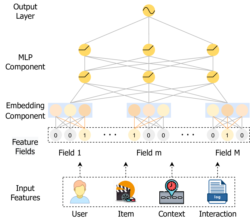
Figure 1. The Typically DLRS architecture.

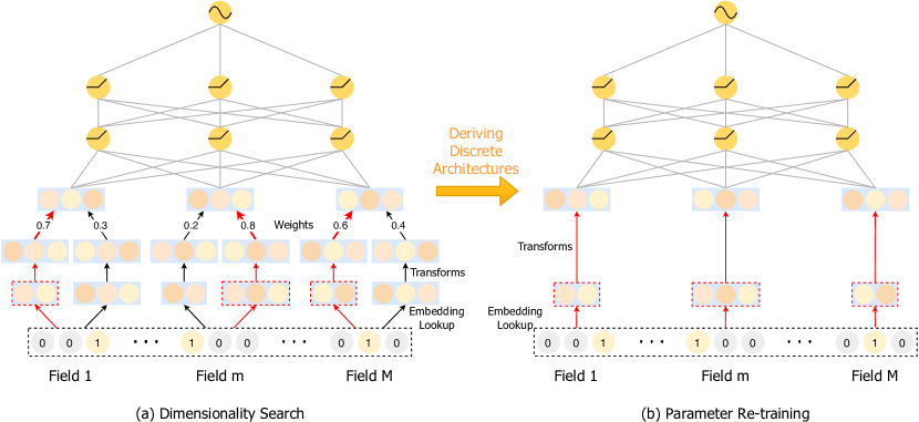
Figure 2. Overview of the proposed framework.

Real-world recommender systems typically involve a massive amount of categorical feature fields from users (e.g. occupation and userID), items (e.g. category and itemID), contextual information (e.g. time and location), and their interactions (e.g. user’s purchase history of items). DLRSs first map these categorical features into real-valued dense vectors via an embedding-component (Pan et al., 2018; Qu et al., 2016; Zhou et al., 2018), i.e., the embedding-lookup process, which leads to huge amounts of embedding parameters. For instance, the YouTube recommender system consists of 1 million of unique videoIDs, and assign each videoID with a specific 256-dimensional embedding vector; in other words, the videoID feature field alone occupies 256 million parameters (Covington et al., 2016). Then, the DLRSs nonlinearly transform the input embeddings from all feature fields and generate the outputs (predictions) via the MLP-component (Multi-Layer Perceptron), which usually involves only several fully connected layers in practice. Therefore, compared to the MLP-component, the embedding-component dominates the number of parameters in practical recommender systems, which naturally plays a tremendously impactful role in the recommendations.

The majority of existing recommender systems assign fixed and unified embedding dimension for all feature fields, such as the famous Wide&Deep model (Cheng et al., 2016), which may lead to memory inefficiency. First, the embedding dimension often determines the capacity to encode information. Thus, allocating the same dimension to all feature fields may lose the information of high predictive features while wasting memory on non-predictive features. Therefore, we should assign large dimension to the high informative and predictive features, for instance, the “location” feature in location-based recommender systems (Bao et al., 2015). Second, different feature fields have different cardinality (i.e. the number of unique values). For example, the gender feature has only two (i.e. male and female), while the itemID feature usually involves millions of unique values. Intuitively, we should allocate larger dimensions to the feature fields with more unique feature values to encode their complex relationships with other features, and assign smaller dimensions to feature fields with smaller cardinality to avoid the overfitting problem due to the over-parameterization (Joglekar et al., 2019; Ginart et al., 2019; Zhao et al., 2020; Kang et al., 2020). According to the above reasons, it is highly desired to assign different embedding dimensions to different feature fields in a memory-efficient manner.

In this paper, we aim to enable different embedding dimensions for different feature fields for recommendations. We face tremendous challenges. First, the relationship among embedding dimensions, feature distributions and neural network architectures is highly intricate, which makes it hard to manually assign embedding dimensions to each feature field (Ginart et al., 2019). Second, real-world recommender systems often involve hundreds and thousands of feature fields. It is difficult, if possible, to artificially select different dimensions for all feature fields, due to the expensive computation cost from the incredibly huge ($N^{M}$, with $N$ the number of candidate dimensions for each feature field to select, and $M$ the number of feature fields) search space. Our attempt to address these challenges results in an end-to-end differentiable AutoML based framework (AutoDim), which can efficiently allocate embedding dimensions to different feature fields in an automated and data-driven manner. Our experiments on benchmark datasets demonstrate the effectiveness of the proposed framework. We summarize our major contributions as: (i) we propose an end-to-end AutoML based framework AutoDim, which can automatically select various embedding dimensions to different feature fields; (ii) we develop two embedding lookup methods and two embedding transformation approaches, and compare the impact of their combinations on the embedding dimension allocation decision; and (iii) we demonstrate the effectiveness of the proposed framework on real-world benchmark datasets.

The rest of this paper is organized as follows. In Section 2, we introduce details about how to assign various embedding dimensions for different feature fields in an automated and data-driven fashion, and propose an AutoML based optimization algorithm. Section 3 carries out experiments based on real-world datasets and presents experimental results. Section 4 briefly reviews related work. Finally, section 5 concludes this work and discusses our future work.

2. Framework

In order to achieve the automated allocation of different embedding dimensions to different feature fields, we propose an AutoML based framework, which effectively addresses the challenges we discussed in Section 1. In this section, we will first introduce the overview of the whole framework; then we will propose an end-to-end differentiable model with two embedding-lookup methods and two embedding dimension search methods, which can compute the weights of different dimensions for feature fields in a soft and continuous fashion, and we will provide an AutoML based optimization algorithm; finally, we will derive a discrete embedding architecture upon the maximal weights, and retrain the whole DLRS framework.

2.1. Overview

Our goal is to assign different feature fields various embedding dimensions in an automated and data-driven manner, so as to enhance the memory efficiency and the performance of the recommender system. We illustrate the overall framework in Figure 2, which consists of two major stages:

2.1.1. Dimensionality search stage

It aims to find the optimal embedding dimension for each feature field. To be more specific, we first assign a set of candidate embeddings with different dimensions to a specific categorical feature via an embedding-lookup step; then, we unify the dimensions of these candidate embeddings through a transformation step, which is because of the fixed input dimension of the first MLP layer; next, we obtain the formal embedding for this categorical feature by computing the weighted sum of all its transformed candidate embeddings, and feed it into the MLP-component. The DLRS parameters including the embeddings and MLP layers are learned upon the training set, while the architectural weights over the candidate embeddings are optimized upon the validation set, which prevents the framework selecting the embedding dimensions that overfit the training set (Pham et al., 2018; Liu et al., 2018a).

In practice, before the alternative training of DLRS parameters and architectural weights, we initially assign equivalent architectural weights on all candidate embeddings (e.g., $[0.5,0.5]$ for the example in Figure 2), fix these architectural weights and pre-train the DLRS including all candidate embeddings. The pre-training enables a fair competition between candidate embeddings when we start to update architectural weights.

2.1.2. Parameter re-training stage

According to the architectural weights learned in dimensionality search stage, we select the embedding dimension for each feature field, and re-train the parameters of DLRS parameters (i.e., MLPs and selected embeddings) on the training dataset in an end-to-end fashion. It is noteworthy that: (i) re-training stage is necessary, since in dimensionality search stage, the model performance is also influenced by the suboptimal embedding dimensions, which are not desired in practical recommender system; and (ii) new embeddings are still unified into the same dimension, since most existing deep recommender models (such as FM (Rendle, 2010), DeepFM (Guo et al., 2017), NFM (He and Chua, 2017)) capture the interactions between two feature fields via a interaction operation (e.g., inner product) over their embedding vectors. These interaction operations constrain the embedding vectors to have same dimensions.

Note that numerical features will be converted into categorical features through bucketing, and we omit this process in the following sections for simplicity. Next, we will introduce the details of each stage.

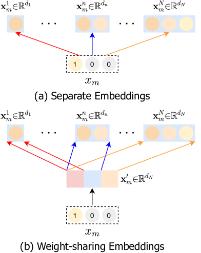
Figure 3. The embedding lookup methods.

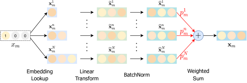
Figure 4. Method 1 - Linear Transformation.

2.2. Dimensionality Search

As discussed in Section 1, different feature fields have different cardinalities and various contributions to the final prediction. Inspired by this phenomenon, it is highly desired to enable various embedding dimensions for different feature fields. However, due to a large amount of feature fields and the complex relationship between embedding dimensions with feature distributions and neural network architectures, it is difficult to manually select embedding dimensions via conventional dimension reduction methods. An intuitive solution to tackle this challenge is to assign several embedding spaces with various dimensions to each feature field, and then the DLRS automatically selects the optimal embedding dimension for each feature field.

2.2.1. Embedding Lookup Tricks

Suppose for each user-item interaction instance, we have $M$ input features $(x_{1},\cdots,x_{M})$, and each feature $x_{m}$ belongs to a specific feature field, such as gender and age, etc. For the $m^{th}$ feature field, we assign $N$ candidate embedding spaces $\{\mathbf{X}_{m}^{1},\cdots,\mathbf{X}_{m}^{N}\}$. The dimension of an embedding in each space is $d_{1},\cdots,d_{N}$, where $d_{1}\textless\cdots\textless d_{N}$; and the cardinality of these embedding spaces are the number of unique feature values in this feature field. Correspondingly, we define $\{\mathbf{x}_{m}^{1},\cdots,\mathbf{x}_{m}^{N}\}$ as the set of candidate embeddings for a given feature $x_{m}$ from all embedding spaces, as shown in Figure 3 (a). Note that we assign the same candidate dimension to all feature fields for simplicity, but it is straightforward to introduce different candidate sets. Therefore, the total space assigned to the feature $x_{m}$ is $\sum_{n=1}^{N}d_{n}$. However, in real-world recommender systems with thousands of feature fields, two challenges lie in this design include (i) this design needs huge space to store all candidate embeddings, and (ii) the training efficiency is reduced since a large number of parameters need to be learned.

To address these challenges, we propose an alternative solution for large-scale recommendations, named weight-sharing embedding architecture. As illustrated in Figure 3 (b), we only allocate a $d_{N}$-dimensional embedding to a given feature $x_{m}$, referred as to $\mathbf{x}_{m}^{\prime}$, then the $n^{th}$ candidate embedding $\mathbf{x}_{m}^{n}$ corresponds to the first $d_{n}$ digits of $\mathbf{x}_{m}^{\prime}$. The advantages associated with weight-sharing embedding method are two-fold, i.e., (i) it is able to reduce the storage space and increase the training efficiency, as well as (ii) since the relatively front digits of $\mathbf{x}_{m}^{\prime}$ have more chances to be retrieved and then be trained (e.g. the “red part” of $\mathbf{x}_{m}^{\prime}$ is leveraged by all candidates in Figure 3 (b)), we intuitively wish they can capture more essential information of the feature $x_{m}$.

2.2.2. Unifying Various Dimensions

Since the input dimension of the first MLP layer in existing DLRSs is often fixed, it is difficult for them to handle various candidate dimensions. Thus we need to unify the embeddings $\{\mathbf{x}_{m}^{1},\cdots,\mathbf{x}_{m}^{N}\}$ into same dimension, and we develop two following methods:

Method 1: Linear Transformation

Figure 4 (a) illustrates the linear transformation method to handle the various embedding dimensions (the difference of two embedding lookup methods is omitted here). We introduce $N$ fully-connected layers, which transform embedding vectors $\{\mathbf{x}_{m}^{1},\cdots,\mathbf{x}_{m}^{N}\}$ into the same dimension $d_{N}$:

(1) $$\begin{array}[]{l}{\mathbf{\widetilde{x}}_{m}^{n}\leftarrow\mathbf{W}_{n}^{\top}\mathbf{x}_{m}^{n}+\mathbf{b}_{n}}\quad\forall n\in[1,N]\end{array}$$

where $\mathbf{W}_{n}\in\mathbb{R}^{d_{n}\times d_{N}}$ is weight matrice and $\mathbf{b}_{n}\in\mathbb{R}^{d_{N}}$ is bias vector. For each field, all candidate embeddings with the same dimension share the same weight matrice and bias vector, which can reduce the amount of model parameters. With the linear transformations, we map the original embedding vectors $\{\mathbf{x}_{m}^{1},\cdots,\mathbf{x}_{m}^{N}\}$ into the same dimensional space, i.e., $\{\mathbf{\widetilde{x}}_{m}^{1},\cdots,\mathbf{\widetilde{x}}_{m}^{N}\}\in\mathbb{R}^{d_{N}}$. In practice, we can observe that the magnitude of the transformed embeddings $\{\mathbf{\widetilde{x}}_{m}^{1},\cdots,\mathbf{\widetilde{x}}_{m}^{N}\}$ varies significantly, which makes them become incomparable. To tackle this challenge, we conduct BatchNorm (Ioffe and Szegedy, 2015) on the transformed embeddings $\{\mathbf{\widetilde{x}}_{m}^{1},\cdots,\mathbf{\widetilde{x}}_{m}^{N}\}$ as:

(2) $$\begin{array}[]{l}\mathbf{\widehat{x}}_{m}^{n}\leftarrow\frac{\mathbf{\widetilde{x}}_{m}^{n}-\mu_{\mathcal{B}}^{n}}{\sqrt{(\sigma_{\mathcal{B}}^{n})^{2}+\epsilon}}\quad\forall n\in[1,N]\end{array}$$

where $\mu_{\mathcal{B}}^{n}$ is the mini-batch mean and $(\sigma_{\mathcal{B}}^{n})^{2}$ is the mini-batch variance for $\forall n\in[1,N]$. $\epsilon$ is a small constant added to the mini-batch variance for numerical stability when $(\sigma_{\mathcal{B}}^{n})^{2}$ is very small. After BatchNorm, the linearly transformed embeddings $\{\mathbf{\widetilde{x}}_{m}^{1},\cdots,\mathbf{\widetilde{x}}_{m}^{N}\}$ become to magnitude-comparable embedding vectors $\{\mathbf{\widehat{x}}_{m}^{1},\cdots,\mathbf{\widehat{x}}_{m}^{N}\}$ with the same dimension $d_{N}$.

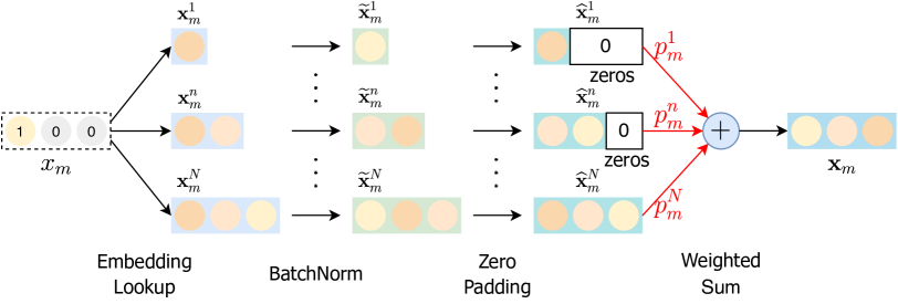
Figure 5. Method 2 - Zero Padding Transformation.

Method 2: Zero Padding

Inspired by zero-padding techniques from the computer version community, which pads the input volume with zeros around the border, we address the problem of various embedding dimensions by padding shorter embedding vectors to the same length as the longest embedding dimension $d_{N}$ with zeros, which is illustrated in Figure 5. For the embedding vectors $\{\mathbf{x}_{i}^{1},\cdots,\mathbf{x}_{i}^{N}\}$ with different dimensions, we first execute BatchNorm process, which forces the original embeddings $\{\mathbf{x}_{i}^{1},\cdots,\mathbf{x}_{i}^{N}\}$ into becoming magnitude-comparable embeddings:

(3) $$\begin{array}[]{l}\mathbf{\widetilde{x}}_{m}^{n}\leftarrow\frac{\mathbf{x}_{m}^{n}-\mu_{\mathcal{B}}^{n}}{\sqrt{(\sigma_{\mathcal{B}}^{n})^{2}+\epsilon}}\quad\forall n\in[1,N]\end{array}$$

where $\mu_{\mathcal{B}}^{n}$, $(\sigma_{\mathcal{B}}^{n})^{2}$ are the mini-batch mean and variance. $\epsilon$ is the constant for numerical stability. The transformed $\{\mathbf{\widetilde{x}}_{m}^{1},\cdots,\mathbf{\widetilde{x}}_{m}^{N}\}$ are magnitude-comparable embeddings. Then we pad the $\{\mathbf{\widetilde{x}}_{m}^{1},\cdots,\mathbf{\widetilde{x}}_{m}^{N-1}\}$ to the same length $d_{N}$ by zeros:

(4) $$\begin{array}[]{l}\,\,\,\,\,{\mathbf{\widehat{x}}_{m}^{n}\leftarrow padding(\,\mathbf{\widetilde{x}}_{m}^{n}\,,\,d_{N}-d_{n})}\quad\forall n\in[1,N]\end{array}$$

where the second term of each padding formula is the number of zeros to be padded with the embedding vector of the first term. Then the embeddings $\{\mathbf{\widehat{x}}_{m}^{1},\cdots,\mathbf{\widehat{x}}_{m}^{N}\}$ share the same dimension $d_{N}$. Compared with the linear transformation (method 1), the zero-padding method reduces lots of linear-transformation computations and corresponding parameters. The possible drawback is that the final embeddings $\{\mathbf{\widehat{x}}_{m}^{1},\cdots,\mathbf{\widehat{x}}_{m}^{N}\}$ becomes spatially unbalanced since the tail parts of some final embeddings are zeros. Next, we will introduce embedding dimension selection process.

2.2.3. Dimension Selection

In this paper, we aim to select the optimal embedding dimension for each feature field in an automated and data-driven manner. This is a hard (categorical) selection on the candidate embedding spaces, which will make the whole framework not end-to-end differentiable. To tackle this challenge, in this work, we approximate the hard selection over different dimensions via introducing the Gumbel-softmax operation (Jang et al., 2016), which simulates the non-differentiable sampling from a categorical distribution by a differentiable sampling from the Gumbel-softmax distribution.

To be specific, suppose weights $\{\alpha_{m}^{1},\cdots,\alpha_{m}^{N}\}$ are the class probabilities over different dimensions. Then a hard selection $z$ can be drawn via the the gumbel-max trick (Gumbel, 1948) as:

(5) $$z= \;\text{one\_hot}\left(\arg\max_{n\in[1,N]}\left[\log\alpha_{m}^{n}+g_{n}\right]\right)$$

$$where\;g_{n}=-\log\left(-\log\left(u_{n}\right)\right)$$

$$\quad\quad\;\;\,u_{n}\sim Uniform(0,1)$$

The gumbel noises $g_{i},\cdots,g_{N}$ are i.i.d samples, which perturb $\log\alpha_{m}^{n}$ terms and make the $\arg\max$ operation that is equivalent to drawing a sample by $\alpha_{m}^{1},\cdots,\alpha_{m}^{N}$ weights. However, this trick is non-differentiable due to the $\arg\max$ operation. To deal with this problem, we use the softmax function as a continuous, differentiable approximation to $\arg\max$ operation, i.e., straight-through gumbel-softmax (Jang et al., 2016):

(6) $$p_{m}^{n}=\frac{\exp\left(\frac{\log\left(\alpha_{m}^{n}\right)+g_{n}}{\tau}\right)}{\sum_{i=1}^{N}\exp\left(\frac{\log\left(\alpha_{m}^{i}\right)+g_{i}}{\tau}\right)}$$

where $\tau$ is the temperature parameter, which controls the smoothness of the output of gumbel-softmax operation. When $\tau$ approaches zero, the output of the gumbel-softmax becomes closer to a one-hot vector. Then $p_{m}^{n}$ is the probability of selecting the $n^{th}$ candidate embedding dimension for the feature $x_{m}$, and its embedding $\mathbf{x}_{m}$ can be formulated as the weighted sum of $\{\mathbf{\widehat{x}}_{m}^{1},\cdots,\mathbf{\widehat{x}}_{m}^{N}\}$:

(7) $$\begin{array}[]{l}\mathbf{x}_{m}=\sum_{n=1}^{N}p_{m}^{n}\cdot\mathbf{\widehat{x}}_{m}^{n}\quad\forall m\in[1,M]\end{array}$$

We illustrate the weighted sum operations in Figure 4 and 5. With gumbel-softmax operation, the dimensionality search process is end-to-end differentiable. The discrete embedding dimension selection conducted based on the weights $\{\alpha_{m}^{n}\}$ will be detailed in the following subsections.

Then, we concatenate the embeddings $\mathbf{h}_{0}=\left[\mathbf{x}_{1},\cdots,\mathbf{x}_{M}\right]$ and feed $\mathbf{h}_{0}$ input into $L$ multilayer perceptron layers:

(8) $$\begin{array}[]{l}{\mathbf{h}_{l}=\sigma\left(\mathbf{W}_{l}^{\top}\mathbf{h}_{l-1}+\mathbf{b}_{l}\right)}\quad\forall l\in[1,L]\end{array}$$

where $\mathbf{W}_{l}$ and $\mathbf{b}_{l}$ are the weight matrix and the bias vector for the $l^{th}$ MLP layer. $\sigma(\cdot)$ is the activation function such as ReLU and Tanh. Finally, the output layer that is subsequent to the last MLP layer, produces the prediction of the current user-item interaction instance as:

(9) $${\hat{y}=\sigma\left(\mathbf{W}_{o}^{\top}\mathbf{h}_{L}+\mathbf{b}_{o}\right)}$$

where $\mathbf{W}_{o}$ and $\mathbf{b}_{o}$ are the weight matrix and bias vector for the output layer. Activation function $\sigma(\cdot)$ is selected based on different recommendation tasks, such as Sigmoid function for regression (Cheng et al., 2016), and Softmax for multi-class classification (Tan et al., 2016). Correspondingly, the objective function $\mathcal{L}(\hat{y},y)$ between prediction $\hat{y}$ and ground truth label $y$ also varies based on different recommendation tasks. In this work, we leverage negative log-likelihood function:

(10) $$\mathcal{L}(\hat{y},y)=-y\log\hat{y}-(1-y)\log(1-\hat{y})$$

where $y$ is the ground truth (1 for like or click, 0 for dislike or non-click). By minimizing the objective function $\mathcal{L}(\hat{y},y)$, the dimensionality search framework updates the parameters of all embeddings, hidden layers, and weights $\{\alpha_{m}^{n}\}$ through back-propagation. The high-level idea of the dimensionality search is illustrated in Figure 2 (a), where we omit some details of embedding-lookup, transformations and gumbel-softmax for the sake of simplicity.

2.3. Optimization

In this subsection, we will detail the optimization method of the proposed AutoDim framework. In AutoDim, we formulate the selection over different embedding dimensions as an architectural optimization problem and make it end-to-end differentiable by leveraging the Gumbel-softmax technique. The parameters to be optimized in AutoDim are two-fold, i.e., (i) $\mathbf{W}$: the parameters of the DLRS, including the embedding-component and the MLP-component; (ii) $\boldsymbol{\alpha}$: the weights $\{\alpha_{m}^{n}\}$ on different embedding spaces ($\{p_{m}^{n}\}$ are calculated based on $\{\alpha_{m}^{n}\}$ as in Equation (6)). DLRS parameters $\mathbf{W}$ and architectural weights $\boldsymbol{\alpha}$ can not be optimized simultaneously on training dataset as conventional supervised attention mechanism since the optimization of them are highly dependent on each other. In other words, simultaneously optimization on training dataset may result in model overfitting on the examples from training dataset.

Inspired by the differentiable architecture search (DARTS) techniques (Liu et al., 2018a), $\mathbf{W}$ and $\boldsymbol{\alpha}$ are alternately optimized through gradient descent. Specifically, we alternately update $\mathbf{W}$ by optimizing the loss $\mathcal{L}_{train}$ on the training data and update $\boldsymbol{\alpha}$ by optimizing the loss $\mathcal{L}_{val}$ on the validation data:

(11) $$\min_{\boldsymbol{\alpha}} \mathcal{L}_{val}\big{(}\mathbf{W}^{*}(\boldsymbol{\alpha}),\boldsymbol{\alpha}\big{)}$$

$$s.t. \mathbf{W}^{*}(\boldsymbol{\alpha})=\arg\min_{\mathbf{W}}\mathcal{L}_{train}(\mathbf{W},\boldsymbol{\alpha}^{*})$$

this optimization forms a bilevel optimization problem (Pham et al., 2018), where architectural weights $\boldsymbol{\alpha}$ and DLRS parameters $\mathbf{W}$ are identified as the upper-level variable and lower-level variable. Since the inner optimization of $\mathbf{W}$ is computationally expensive, directly optimizing $\boldsymbol{\alpha}$ via Eq.(11) is intractable. To address this challenge, we take advantage of the approximation scheme of DARTS:

Algorithm 1 DARTS based Optimization for AutoDim.

Input: the features $(x_{1},\cdots,x_{M})$ of user-item interactions and the corresponding ground-truth labels $y$
Output: the well-learned DLRS parameters $\mathbf{W}^{*}$; the well-learned weights on various embedding spaces $\boldsymbol{\alpha}^{*}$

1:  while not converged do

2:     Sample a mini-batch of user-item interactions from validation data

3:     Update $\boldsymbol{\alpha}$ by descending $\nabla_{\boldsymbol{\alpha}}\;\mathcal{L}_{val}\big{(}\mathbf{W}^{*}(\boldsymbol{\alpha}),\boldsymbol{\alpha}\big{)}$ with the approximation in Eq.(LABEL:equ:approximation)

4:     Collect a mini-batch of training data

5:     Generate predictions $\hat{y}$ via DLRS with current $\mathbf{W}$ and architectural weights $\boldsymbol{\alpha}$

6:     Update $\mathbf{W}$ by descending $\nabla_{\mathbf{W}}\mathcal{L}_{train}(\mathbf{W},\boldsymbol{\alpha})$

7:  end while

(12) $$\arg\min_{\mathbf{W}}\mathcal{L}_{train}(\mathbf{W},\boldsymbol{\alpha}^{*})\approx\mathbf{W}-\xi\nabla_{\mathbf{W}}\mathcal{L}_{train}(\mathbf{W},\boldsymbol{\alpha})$$

where $\xi$ is the learning rate. In the approximation scheme, when updating $\boldsymbol{\alpha}$ via Eq.(LABEL:equ:approximation), we estimate $\mathbf{W}^{*}(\boldsymbol{\alpha})$ by descending the gradient $\nabla_{\mathbf{W}}\mathcal{L}_{train}(\mathbf{W},\boldsymbol{\alpha})$ for only one step, rather than to optimize $\mathbf{W}(\boldsymbol{\alpha})$ thoroughly to obtain $\mathbf{W}^{*}(\boldsymbol{\alpha})=\arg\min_{\mathbf{W}}$ $\mathcal{L}_{train}(\mathbf{W},\boldsymbol{\alpha}^{*})$. In practice, it usually leverages the first-order approximation by setting $\xi=0$, which can further enhance the computation efficiency.

The DARTS based optimization algorithm for AutoDim is detailed in Algorithm 1. Specifically, in each iteration, we first sample a batch of user-item interaction data from the validation set (line 2); next, we update the architectural weights $\boldsymbol{\alpha}$ upon it (line 3); afterward, the DLRS make the predictions $\hat{y}$ on the batch of training data with current DLRS parameters $\mathbf{W}$ and architectural weights $\boldsymbol{\alpha}$ (line 5); eventually, we update the DLRS parameters $\mathbf{W}$ by descending $\nabla_{\mathbf{W}}\mathcal{L}_{train}(\mathbf{W},\boldsymbol{\alpha})$ (line 6).

2.3.1. A pre-train trick.

In practice, in order to enable a fair competition between the candidate embeddings, for each feature field, we first allocate the equivalent architectural weights initially on all its candidate embeddings, e.g., $[0.5,0.5]$ if there are two candidate embedding dimensions. Then, we fix these initialized architectural weights $\boldsymbol{\alpha}$ and pre-train the DLRS parameters $\mathbf{W}$ including all candidate embeddings. This process ensures a fair competition between candidate embeddings when we begin to update $\boldsymbol{\alpha}$.

2.4. Parameter Re-Training

Since the suboptimal embedding dimensions in dimensionality search stage also influence the model training, a re-training stage is desired to training the model with only optimal dimensions, which can eliminate these suboptimal influences. In this subsection, we will introduce how to select optimal embedding dimension for each feature field and the details of re-training the recommender system with the selected embedding dimensions.

2.4.1. Deriving Discrete Dimensions

During re-training, the gumbel-softmax operation is no longer used, which means that the optimal embedding space (dimension) are selected for each feature field as the one corresponding to the largest weight, based on the well-learned $\boldsymbol{\alpha}$. It is formally defined as:

(13) $$\begin{array}[]{l}\;\mathbf{X}_{m}=\mathbf{X}_{m}^{k},\;\;\;where\;\;k=\arg\max_{n\in[1,N]}\alpha_{m}^{n}\quad\forall m\in[1,M]\end{array}$$

Figure 2 (a) illustrates the architecture of AutoDim framework with a toy example about the optimal dimension selections based on two candidate dimensions, where the largest weights corresponding to the $1^{st}$, $m^{th}$ and $M^{th}$ feature fields are $0.7$, $0.8$ and $0.6$, then the embedding space $\mathbf{X}_{1}^{1}$, $\mathbf{X}_{m}^{2}$ and $\mathbf{X}_{M}^{1}$ are selected for these feature fields. The dimension of an embedding vector in these embedding spaces is $d_{1}$, $d_{2}$ and $d_{1}$, respectively.

Algorithm 2 The Optimization of DLRS Re-training Process.

Input: the features $(x_{1},\cdots,x_{M})$ of user-item interactions and the corresponding ground-truth labels $y$
Output: the well-learned DLRS parameters $\mathbf{W}^{*}$

1:  while not converged do

2:     Sample a mini-batch of training data

3:     Generate predictions $\hat{y}$ via DLRS with current $\mathbf{W}$

4:     Update $\mathbf{W}$ by descending $\nabla_{\mathbf{W}}\mathcal{L}_{train}(\mathbf{W})$

5:  end while

2.4.2. Model Re-training

As shown in Figure 2 (b), given the selected embedding spaces, we can obtain unique embedding vectors $(\mathbf{x}_{1},\cdots,\mathbf{x}_{M})$ for features $(x_{1},\cdots,x_{M})$. Then we concatenate these embeddings and feeds them into hidden layers. Next, the prediction $\hat{y}$ is generated by the output layer. Finally, all the parameters of the DLRS, including embeddings and MLPs, will be updated via minimizing the supervised loss function $\mathcal{L}(\hat{y},y)$ through back-propagation. The model re-training algorithm is detailed in Algorithm 2. The re-training process is based on the same training data as Algorithm 1.

Note that the majority of existing deep recommender algorithms (such as FM (Rendle, 2010), DeepFM (Guo et al., 2017), FFM (Pan et al., 2018), AFM (Xiao et al., 2017), xDeepFM (Lian et al., 2018)) capture the interactions between feature fields via interaction operations, such as inner product and Hadamard product. These interaction operations require the embedding vectors from all fields to have the same dimensions. Therefore, the embeddings selected in Section 2.4.1 are still mapped into the same dimension as in Section 2.2.2. In the re-training stage, the BatchNorm operation is no longer in use, since there are no comparisons between candidate embeddings in each field. Unifying embeddings into the same dimension does not increase model parameters and computations too much: (i) linear transformation: all embeddings from one feature field share the same weight matrice and bias vector, and (ii) zero-padding: no extra trainable parameters are introduced.

3. Experiments

In this section, we first introduce experimental settings. Then we conduct extensive experiments to evaluate the effectiveness of the proposed AutoDim framework. We mainly seek answers to the following research questions: RQ1: How does AutoDim perform compared with other embedding dimension search methods? RQ2: How do the important components, i.e., 2 embedding lookup methods and 2 transformation methods, influence the performance? RQ3: How efficient is AutoDim as compared with other methods? RQ4: What is the impact of important parameters on the results? RQ5: What is the transferability and stability of AutoDim? RQ6: Can AutoDim assign large embedding dimensions to really important feature fields?

Table 1. Statistics of the datasets.

Data	Criteo	Avazu
# Interactions	45,840,617	40,428,968
# Feature Fields	39	22
# Sparse Features	1,086,810	2,018,012

Table 2. Performance comparison of different embedding search methods

Dataset	Model	Metrics	Search Methods
			FDE	MDE	DPQ	NIS	MGQE	AutoEmb	RaS	AutoDim-s	AutoDim
Criteo	FM	AUC	0.8020	0.8027	0.8035	0.8042	0.8046	0.8049	0.8056	0.8063	0.8078*
		Logloss	0.4487	0.4481	0.4472	0.4467	0.4462	0.4460	0.4457	0.4452	0.4438*
		Params (M)	34.778	15.520	20.078	13.636	12.564	13.399	16.236	31.039	11.632*
Criteo	W&D	AUC	0.8045	0.8051	0.8058	0.8067	0.8070	0.8072	0.8076	0.8081	0.8098*
		Logloss	0.4468	0.4464	0.4457	0.4452	0.4446	0.4445	0.4443	0.4439	0.4419*
		Params (M)	34.778	18.562	22.628	14.728	15.741	15.987	18.233	30.330	12.455*
Criteo	DeepFM	AUC	0.8056	0.8060	0.8067	0.8076	0.8080	0.8082	0.8085	0.8089	0.8101*
		Logloss	0.4457	0.4456	0.4449	0.4442	0.4439	0.4438	0.4436	0.4432	0.4416*
		Params (M)	34.778	17.272	25.737	12.955	13.059	13.437	17.816	31.770	11.457*
Avazu	FM	AUC	0.7799	0.7802	0.7809	0.7818	0.7823	0.7825	0.7827	0.7831	0.7842*
		Logloss	0.3805	0.3803	0.3799	0.3792	0.3789	0.3788	0.3787	0.3785	0.3776*
		Params (M)	64.576	22.696	28.187	22.679	22.769	21.026	27.272	55.038	17.595*
Avazu	W&D	AUC	0.7827	0.7829	0.7836	0.7842	0.7849	0.7851	0.7853	0.7856	0.7872*
		Logloss	0.3788	0.3785	0.3777	0.3772	0.3768	0.3767	0.3767	0.3766	0.3756*
		Params (M)	64.576	27.976	35.558	21.413	19.457	17.292	35.126	56.401	14.130*
Avazu	DeepFM	AUC	0.7842	0.7845	0.7852	0.7858	0.7863	0.7866	0.7867	0.7870	0.7881*
		Logloss	0.3742	0.3739	0.3737	0.3736	0.3734	0.3733	0.3732	0.3730	0.3721*
		Params (M)	64.576	32.972	36.128	22.550	17.575	21.605	29.235	58.325	13.976*

“*” indicates the statistically significant improvements (i.e., two-sided t-test with $p<0.05$) over the best baseline. (M=Million)

3.1. Datasets

We evaluate our model on two benchmark datasets: (i) Criteo: This is a benchmark industry dataset to evaluate ad click-through rate prediction models. It consists of 45 million users’ click records on displayed ads over one month. For each data example, it contains 13 numerical feature fields and 26 categorical feature fields. We normalize numerical features by transforming a value $v\rightarrow\left\lfloor\log(v)^{2}\right\rfloor$ if $v>2$ as proposed by the Criteo Competition winner , and then convert it into categorical features through bucketing. All $M=39$ feature fields are anonymous. (ii) Avazu: Avazu dataset was provided for the CTR prediction challenge on Kaggle, which contains 11 days’ user clicking behaviors that whether a displayed mobile ad impression is clicked or not. There are $M=22$ categorical feature fields including user/ad features and device attributes. Parts of the fields are anonymous. Some key statistics of the datasets are shown in Table 1. For each dataset, we use 90% user-item interactions as the training/validation set (8:1), and the rest 10% as the test set.

3.2. Implement Details

Next, we detail the AutoDim architectures. For the DLRS, (i) embedding component: existing work usually set the embedding dimension as 10 or 16, while recent research found that a larger embedding size leads to better performance (Zhu et al., 2020), so we set the maximal embedding dimension as 32 within our GPU memory constraints. For each feature field, we select from $N=5$ candidate embedding dimensions $\{2,8,16,24,32\}$. (ii) MLP component: we have two hidden layers with the size $|h_{0}|\times 128$ and $128\times 128$, where $|h_{0}|$ is the input size of first hidden layer, $|h_{0}|=32\times M$ with $M$ the number of feature fields for different datasets, and we use batch normalization, dropout ($rate=0.2$) and ReLU activation for both hidden layers. The output layer is $128\times 1$ with Sigmoid activation.

For architectural weights $\boldsymbol{\alpha}$: $\alpha_{m}^{1},\cdots,\alpha_{m}^{N}$ of the $m^{th}$ feature field are produced by a Softmax activation upon a trainable vector of length $N$. We use an annealing temperature $\tau=\max(0.01,1-0.00005\cdot t)$ for Gumbel-softmax, where $t$ is the training step.

The learning rate for updating DLRS and weights are $0.001$ and $0.001$, and the batch-size is set as 2000. For the parameters of the proposed AutoDim framework, we select them via cross-validation. Correspondingly, we also do parameter-tuning for baselines for a fair comparison. We will discuss more details about parameter selection for the proposed framework in the following subsections.

Our implementation is based on a public Pytorch for recommendation library, which involves 16 state-of-the-art recommendation algorithms. Our model is implemented as 3 separate classes/functions, so it is easily to be apply our AutoDim model to these recommendation algorithms. Due to the limited space, we show the performances of applying AutoDim on FM (Rendle, 2010), W&D (Cheng et al., 2016) and DeepFM (Guo et al., 2017).

3.3. Evaluation Metrics

The performance is evaluated by AUC, Logloss and Params, where a higher AUC or a lower Logloss indicates a better recommendation performance. A lower Params means a fewer embedding parameters. Area Under the ROC Curve (AUC) measures the probability that a positive instance will be ranked higher than a randomly chosen negative one; we introduce Logoss since all methods aim to optimize the logloss in Equation (10), thus it is natural to utilize Logloss as a straightforward metric. It is noteworthy that a slightly higher AUC or lower Logloss at 0.001-level is regarded as significant for the CTR prediction task (Cheng et al., 2016; Guo et al., 2017). For an embedding dimension search model, the Params metric is the optimal number of embedding parameters selected by this model for the recommender system. We omit the number of MLP parameters, which only occupy a small part of the total model parameters, e.g., $\sim 0.5\%$ in W&D and DeepFM on Criteo dataset. FM model has no MLP component.

3.4. Overall Performance (RQ1)

We compare the proposed framework with following embedding dimension search methods: (i) FDE (Full Dimension Embedding): In this baseline, we assign the same embedding dimensions to all feature fields. For each feature field, the embedding dimension is set as the maximal size from the candidate set, i.e., 32. (ii) MDE (Mixed Dimension Embedding) (Ginart et al., 2019): This is a heuristic method that assigns highly-frequent feature values with larger embedding dimensions, vice versa. We enumerate its 16 groups of suggested hyperparameters settings and report the best one. (iii) DPQ (Differentiable Product Quantization) (Chen et al., 2019): This baseline introduces differentiable quantization techniques from network compression community to compact embeddings. (iv) NIS (Neural Input Search) (Joglekar et al., 2020): This baseline applies reinforcement learning to learn to allocate larger embedding sizes to active feature values, and smaller sizes to inactive ones. (v) MGQE (Multi-granular quantized embeddings) (Kang et al., 2020): This baseline is based on DPQ, and further cuts down the embeddings space by using fewer centroids for non-frequent feature values. (vi) AutoEmb (Automated Embedding Dimensionality Search) (Zhao et al., 2020): This baseline is based on DARTS (Liu et al., 2018a), and assigns embedding dimensions according to the frequencies of feature values. (vii) RaS (Random Search): Random search is strong baseline in neural network search (Liu et al., 2018a). We apply the same candidate embedding dimensions, randomly allocate dimensions to feature fields in each experiment time, and report the best performance. (viii) AutoDim-s: This baseline shares the same architecture with AutoDim, while we update the DLRS parameters and architectural weights simultaneously on the same training batch in an end-to-end backpropagation fashion.

The overall results are shown in Table 2. We can observe: (1) FDE achieves the worst recommendation performance and largest Params, where FDE is assigned the maximal embedding dimension 32 to all feature fields. This result demonstrates that allocating same dimension to all feature fields is not only memory inefficient, but introduces numerous noises into the model. (2) RaS, AutoDim-s, AutoDim performs better than MDE, DPQ, NIS, MGQE, AutoEmb. The major differences between these two groups of methods are: (i) the first group aims to assign different embedding dimensions to different feature fields, while embeddings in the same feature field share the same dimension; (ii) the second group attempts to assign different embedding sizes to different feature values within the same feature fields, which are based on the frequencies of feature values. The second group of methods surfer from several challenges: (ii-a) there are numerous unique values in each feature field, e.g., $2.7\times 10^{4}$ values for each feature field on average in Criteo dataset. This leads to a huge search space (even after bucketing) in each feature field, which makes it difficult to find the optimal solution, while the search space for each feature field is $N=5$ in AutoDim; (ii-b) allocating dimensions solely based on feature frequencies (i.e., how many times a feature value appears in the training set) may lose other important characteristics of the feature; (ii-c) the feature values frequencies are usually dynamic and not pre-known in real-time recommender system, e.g., the cold-start users/items; and (ii-d) it is difficult to manage embeddings with different dimensions for the same feature filed. (3) AutoDim outperforms RaS and AutoDim-s, where AutoDim updates the architectural weights $\boldsymbol{\alpha}$ on the validation batch, which can enhance the generalization; AutoDim-s updates the $\boldsymbol{\alpha}$ with DLRS on the same training batch simultaneously, which may lead to overfitting; RaS randomly search the dimensions, which has a large search space. AutoDim-s has much larger Params than AutoDim, which indicates that larger dimensions are more efficient in minimizing training loss.

To sum up, we can draw an answer to the first question: compared with the representative baselines, AutoDim achieves significantly better recommendation performance, and saves $70\%\sim 80\%$ embedding parameters. These results prove the effectiveness of the AutoDim framework.

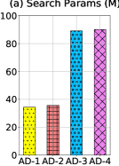
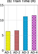
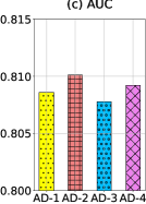
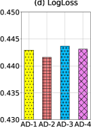
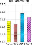
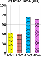
Figure 6. Component analysis of DeepFM on Criteo dataset. *(f) Infer time is averaged for one batch (batch size = 2,000)

3.5. Component Analysis (RQ2)

In this paper, we propose two embedding lookup methods in Section 2.2.1 (i.e. separate embeddings v.s. weight-sharing embeddings) and two transformation methods in Section 2.2.2 (i.e. linear transformation v.s. zero-padding transformation). In this section, we investigate their influence on performance. We systematically combine the corresponding model components by defining the following variants of AutoDim: (i) AD-1: weight-sharing embeddings and zero-padding transformation; (ii) AD-2: weight-sharing embeddings and linear transformation; (iii) AD-3: separate embeddings and zero-padding transformation; (iv) AD-4: separate embeddings and linear transformation.

The results of DeepFM on the Criteo dataset are shown in Figure 6. We omit similar results on other models/datasets due to the limited space. We make the following observations: (1) In Figure 6 (a), we compare the embedding component parameters of in the dimension search stage, i.e., all the candidate embeddings and the transformation neural networks shown in Figure 4 or 5. We can observe that AD-1 and AD-2 save significant model parameters by introducing the weight-sharing embeddings, which also leads to a faster training speed in Figure 6 (b). Therefore, weight-sharing embeddings can benefit real-world recommenders where exist thousands of feature fields and the computing resources are limited. (2) Compared with linear transformation, leveraging zero-padding transformation have slightly fewer parameters, and result in slightly faster training speed (e.g., AD-1 v.s. AD-2 in Figure 6 (a) and (b)). However, we can observe the final DLRS architecture selected by AD-1 loses to that of AD-2 in Figure 6 (c) AUC and (d) Logloss. The reason is that zero-padding embeddings may lose information when conduct inner product. For instance, to compute the inner product of $a=[a_{1},a_{2},a_{3}]$ and $b=[b_{1},b_{2}]$, we first pad $b$ to $b=[b_{1},b_{2},0]$, then $<a,b>=a_{1}\cdot b_{1}+a_{2}\cdot b_{2}+a_{3}\cdot 0$, where the information $a_{3}$ is lost via multiplying 0. Models without element-wise product between embeddings, such as FNN (Zhang et al., 2016), do not suffer from this drawback. (3) In Figure 6 (e) and (f), we can observe that the final embedding dimensions selected by AD-2 save most model parameters and has the fastest inference speed. (4) From Figure 6 (c) and (d), variants with weight-sharing embeddings have better performance than variants using separate embeddings. This is because the relatively front digits of its embedding space are more likely to be recalled and trained (as shown in Figure 3 (b)), which enable the framework capture more essential information in these digits, and make optimal dimension assignment selection.

In summary, we can answer the second question: different component has its advantages, such as zero-padding has fastest training speed and uses least parameters, linear transformation has best performances on AUC/Logloss/Params metrics, and has good training speed and model parameters. If not specified, the results in other subsections are based on the AD-2, and we use linear transformation for RaS and AutoDim-s in Section 3.4.

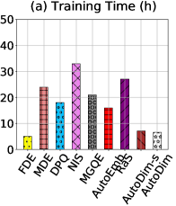
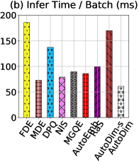
Figure 7. Efficiency analysis of DeepFM on Criteo dataset.

3.6. Efficiency Analysis (RQ3)

In addition to model effectiveness, the training and inference efficiency are also essential metrics for deploying a recommendation model into commercial recommender systems. In this section, we investigate the efficiency of applying search methods to DeepFM on Criteo dataset (on one Tesla K80 GPU). Similar results on other models/dataset are omitted due to the limited space. We illustrate the results in Figure 7.

For the training time in Figure  7 (a), we can observe that AutoDim and AutoDim-s have fast training speed. As discussed in Section 3.4, the reason is that they have a smaller search space than other baselines. FDE’s training is fast since we directly set its embedding dimension as 32, i.e., no searching stage, while its recommendation performance is worst among all methods in Section 3.4. For the inference time, which is more crucial when deploying a model in commercial recommender systems, AutoDim achieves the least inference time as shown in Figure 7 (b). This is because the final recommendation model selected by AutoDim has the least embedding parameters, i.e., the Params metric.

To summarize, AutoDim can efficiently achieve better performance, which makes it easier to be launched in real-world recommender systems.

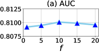
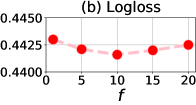
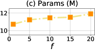
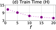
Figure 8. Parameter analysis of DeepFM on Criteo dataset.

3.7. Parameter Analysis (RQ4)

In this section, we investigate how the essential hyper-parameters influence model performance. Besides common hyper-parameters of deep recommender systems such as the number of hidden layers (we omit them due to limited space), our model has one particular hyper-parameter, i.e., the frequency to update architectural weights $\boldsymbol{\alpha}$, referred to as $f$. In Algorithm 1, we alternately update DLRS’s parameters on the training data and update $\boldsymbol{\alpha}$ on the validation data. In practice, we find that updating $\boldsymbol{\alpha}$ can be less frequently than updating DLRS’s parameters, which apparently reduces lots of computations, and also enhances the performance.

To study the impact of $f$, we investigate how DeepFM with AutoDim performs on Criteo dataset with the changes of $f$, while fixing other parameters. Figure 8 shows the parameter sensitivity results, where in $x$-axis, $f=i$ means updating $\boldsymbol{\alpha}$ once, then updating DLRS’s parameters $i$ times. We can observe that the AutoDim achieves the optimal AUC/Logloss when $f=10$. In other words, updating $\boldsymbol{\alpha}$ too frequently/infrequently results in suboptimal performance. Figure 8 (d) shows that setting $f=10$ can reduce $\sim 50\%$ training time compared with setting $f=1$.

Figure 8 (c) shows that lower $f$ leads to lower Params, vice versa. The reason is that AutoDim updates $\boldsymbol{\alpha}$ by minimizing validation loss, which improves the generalization of model (Pham et al., 2018; Liu et al., 2018a). When updating $\boldsymbol{\alpha}$ frequently (e.g., $f=1$), AutoDim tends to select smaller embedding size that has better generalization, while may has under-fitting problem; while when updating $\boldsymbol{\alpha}$ infrequently (e.g., $f=20$), AutoDim prefers larger embedding sizes that perform better on training set, but may lead to over-fitting problem. $f=10$ is a good trade-off between model performance on training and validation sets. Results of the other models/dataset are similar, we omit them because of the limited space.

3.8. Transferability and Stability (RQ5)

3.8.1. Transferability of selected dimensions

In this subsection, we investigate whether the embedding dimensions selected by a simple model (FM with AutoDim, say FM+AD) can be applied to the representative models, such as NFM (He and Chua, 2017), PNN (Qu et al., 2016), AutoInt (Song et al., 2019), to enhance their recommendation performance. From Section 3.4, we know the FM+AD can save $70\%\sim 80\%$ embedding parameters.

The results are shown in Table 3, where ”Model+AD” means assigning the embedding dimensions selected by FM+AD to this Model. We can observe that the performances of three models are significantly improved by applying embedding dimensions selected by FM+AD on two datasets. These observations demonstrate the transferability of embedding dimensions selected by FM+AD.

3.8.2. Stability of selected dimensions

To study whether the dimensions selected by AutoDim are stable, we run the search stage of DeepFM+AutoDim on Criteo dataset with different random seeds. The Pearson correlation of selected dimensions from different seeds is around 0.85, which demonstrates the stability of the selected dimensions.

Table 3. Transferability of selected dimensions.

Model	Criteo		Avazu
	AUC	Logloss	AUC	Logloss
NFM	0.8018	0.4491	0.7741	0.3846
NFM+AD	0.8065*	0.4451*	0.7766*	0.3817*
IPNN	0.8085	0.4428	0.7855	0.3772
IPNN+AD	0.8112*	0.4407*	0.7869*	0.3761*
AutoInt	0.8096	0.4418	0.786	0.3763
AutoInt+AD	0.8116*	0.4403*	0.7875*	0.3756*

“*” indicates the statistically significant improvements (i.e., two-sided t-test with $p<0.05$).

Table 4. Embedding dimensions for Movielens-1m

feature field	W&D (one field)		AutoDim
	AUC	Logloss	Dimension
movieId	0.7321	0.5947	8
year	0.5763	0.6705	2
genres	0.6312	0.6536	4
userId	0.6857	0.6272	8
gender	0.5079	0.6812	2
age	0.5245	0.6805	2
occupation	0.5264	0.6805	2
zip	0.6524	0.6443	4

3.9. Case Study (RQ6)

In this section, we investigate whether AutoDim can assign larger embedding dimensions to more important features. Since feature fields are anonymous in Criteo and Avazu, we apply W&D with AutoDim on MovieLens-1m dataset . MovieLens-1m is a benchmark for evaluating recommendation algorithms, which contains users’ ratings on movies. The dataset includes 6,040 users and 3,416 movies with 1 million user-item interactions. We binarize the ratings into a binary classification task, where ratings of 4 and 5 are viewed as positive and the rest as negative. There are $M=8$ categorical feature fields: movieId, year, genres, userId, gender, age, occupation, zip. Since MovieLens-1m is much smaller than Criteo and Avazu, we set the candidate embedding dimensions as $\{2,4,8,16\}$.

To measure the contribution of a feature field to the final prediction, we build a W&D model with only this field, train this model and evaluate it on the test set. A higher AUC and a lower Logloss means this feature field is more predictive for the final prediction. Then, we build a comprehensive W&D model incorporating all feature fields, and apply AutoDim to select the dimensions for all feature fields. The results are shown in Table 4. It can be observed that: (1) No feature fields are assigned 16-dimensional embedding space, which means candidate embedding dimensions $\{2,4,8,16\}$ are sufficient to cover all possible choices. (2) Compared to the AUC/Logloss of W&D with each feature field, we can find that AutoDim assigns larger embedding dimensions to important (highly predictive) feature fields, such as movieId and userId, vice versa. (3) We build a full dimension embedding (FDE) version of W&D, where all feature fields are assigned as the maximal dimension 16. Its performances are AUC=0.8077, Logloss=0.5383, while the performances of W&D with AutoDim are AUC=0.8113, Logloss=0.5242, and it saves 57% embedding parameters.

In short, above observations validates that AutoDim can assign larger embedding dimensions to more predictive feature fields, which significantly enhances model performance and reduce embedding parameters.

4. Related Work

In this section, we will discuss the related works. We summarize the works related to our research from two perspectives, say, deep recommender systems and AutoML for neural architecture search.

Deep recommender systems have drawn increasing attention from both the academia and the industry thanks to its great advantages over traditional methods (Zhang et al., 2019). Various types of deep learning approaches in recommendation are developed. Sedhain et al. (Sedhain et al., 2015) present an AutoEncoder based model named AutoRec. In their work, both item-based and user-based AutoRec are introduced. They are designed to capture the low-dimension feature embeddings of users and items, respectively. Hidasi et al. (Hidasi et al., 2015) introduce an RNN based recommender system named GRU4Rec. In session-based recommendation, the model captures the information from items’ transition sequences for prediction. They also design a session-parallel mini-batches algorithm and a sampling method for output, which make the training process more efficient. Cheng et al. (Cheng et al., 2016) introduce a Wide&Deep framework for both regression and classification tasks. The framework consists of a wide part, which is a linear model implemented as one layer of a feed-forward neural network, and a deep part, which contains multiple perceptron layers to learn abstract and deep representations. Guo et al. (Guo et al., 2017) propose the DeepFM model. It combines the factorization machine (FM) and MLP. The idea of it is to use the former to model the lower-order feature interactions while using the latter to learn the higher-order interactions. Wang et al. (Wang et al., 2017a) attempt to utilize CNN to extract visual features to help POI (Point-of-Interest) recommendations. They build a PMF based framework that models the interactions between visual information and latent user/location factors. Chen et al. (Chen et al., 2017) introduce hierarchical attention mechanisms into recommendation models. They propose a collaborative filtering model with an item-level and a component-level attention mechanism. The item-level attention mechanism captures user representations by attending various items and the component-level one tries to figure out the most important features from auxiliary sources for each user. Wang et al. (Wang et al., 2017b) propose a generative adversarial network (GAN) based information retrieval model, IRGAN, which is applied in the task of recommendation, and also web search and question answering.

The research of AutoML for neural architecture search can be traced back to NAS (Zoph and Le, 2016), which first utilizes an RNN based controller to design neural networks and proposes a reinforcement learning algorithm to optimize the framework. After that, many endeavors are conducted on reducing the high training cost of NAS. Pham et al. (Pham et al., 2018) propose ENAS, where the controller learns to search a subgraph from a large computational graph to form an optimal neural network architecture. Brock et al. (Brock et al., 2017) introduce a framework named SMASH, in which a hyper-network is developed to generate weights for sampled networks. DARTS (Liu et al., 2018a) and SNAS (Xie et al., 2018) formulate the problem of network architecture search in a differentiable manner and solve it using gradient descent. Luo et al. (Luo et al., 2018) investigate representing network architectures as embeddings. Then they design a predictor to take the architecture embedding as input to predict its performance. They utilize gradient-based optimization to find an optimal embedding and decode it back to the network architecture. Some works raise another way of thinking, which is to limit the search space. The works (Real et al., 2019; Zhong et al., 2018; Liu et al., 2018b; Cai et al., 2018) focus on searching convolution cells, which are stacked repeatedly to form a convolutional neural network. Zoph et al. (Zoph et al., 2018) propose a transfer learning framework called NASNet, which train convolution cells on smaller datasets and apply them on larger datasets. Tan et al. (Tan et al., 2019) introduce MNAS. They propose to search hierarchical convolution cell blocks in an independent manner, so that a deep network can be built based on them. Mixed Dimension Embedding (Ginart et al., 2019), Differentiable Product Quantization (Chen et al., 2019), Neural Input Search (Joglekar et al., 2019; Cheng et al., 2020), Multi-granular Quantized Embedding (Kang et al., 2020), and Automated Embedding Dimensionality Search (Zhao et al., 2020) are designed for tuning the embedding layer of deep recommender system. But they aim to tune the embedding sizes within the same feature field, and we discuss the detailed differences and drawbacks of these models in Section 3.4.

5. Conclusion

In this paper, we propose a novel framework AutoDim, which targets at automatically assigning different embedding dimensions to different feature fields in a data-driven manner. In real-world recommender systems, due to the huge amounts of feature fields and the highly complex relationships among embedding dimensions, feature distributions and neural network architectures, it is difficult, if possible, to manually allocate different dimensions to different feature fields. Thus, we proposed an AutoML based framework to automatically select from different embedding dimensions. To be specific, we first provide an end-to-end differentiable model, which computes the weights over different dimensions for different feature fields simultaneously in a soft and continuous form, and we propose an AutoML-based optimization algorithm; then according to the maximal weights, we derive a discrete embedding architecture, and re-train the DLRS parameters. We evaluate the AutoDim framework with extensive experiments based on widely used benchmark datasets. The results show that our framework can maintain or achieve slightly better performance with much fewer embedding space demands.

References

- (1)
- Bao et al. (2015) Jie Bao, Yu Zheng, David Wilkie, and Mohamed Mokbel. 2015. Recommendations in location-based social networks: a survey. Geoinformatica 19, 3 (2015), 525–565.
- Breese et al. (1998) John S Breese, David Heckerman, and Carl Kadie. 1998. Empirical analysis of predictive algorithms for collaborative filtering. In Proceedings of the Fourteenth conference on Uncertainty in artificial intelligence. Morgan Kaufmann Publishers Inc., 43–52.
- Brock et al. (2017) Andrew Brock, Theodore Lim, James M Ritchie, and Nick Weston. 2017. Smash: one-shot model architecture search through hypernetworks. arXiv preprint arXiv:1708.05344 (2017).
- Cai et al. (2018) Han Cai, Jiacheng Yang, Weinan Zhang, Song Han, and Yong Yu. 2018. Path-level network transformation for efficient architecture search. arXiv preprint arXiv:1806.02639 (2018).
- Chang et al. (2006) Chia-Hui Chang, Mohammed Kayed, Moheb R Girgis, and Khaled F Shaalan. 2006. A survey of web information extraction systems. IEEE transactions on knowledge and data engineering 18, 10 (2006), 1411–1428.
- Chen et al. (2017) Jingyuan Chen, Hanwang Zhang, Xiangnan He, Liqiang Nie, Wei Liu, and Tat-Seng Chua. 2017. Attentive collaborative filtering: Multimedia recommendation with item-and component-level attention. In Proceedings of the 40th International ACM SIGIR conference on Research and Development in Information Retrieval. 335–344.
- Chen et al. (2019) Ting Chen, Lala Li, and Yizhou Sun. 2019. Differentiable product quantization for end-to-end embedding compression. arXiv preprint arXiv:1908.09756 (2019).
- Cheng et al. (2016) Heng-Tze Cheng, Levent Koc, Jeremiah Harmsen, Tal Shaked, Tushar Chandra, Hrishi Aradhye, Glen Anderson, Greg Corrado, Wei Chai, Mustafa Ispir, et al. 2016. Wide & deep learning for recommender systems. In Proceedings of the 1st workshop on deep learning for recommender systems. ACM, 7–10.
- Cheng et al. (2020) Weiyu Cheng, Yanyan Shen, and Linpeng Huang. 2020. Differentiable Neural Input Search for Recommender Systems. arXiv preprint arXiv:2006.04466 (2020).
- Covington et al. (2016) Paul Covington, Jay Adams, and Emre Sargin. 2016. Deep neural networks for youtube recommendations. In Proceedings of the 10th ACM conference on recommender systems. 191–198.
- Ginart et al. (2019) Antonio Ginart, Maxim Naumov, Dheevatsa Mudigere, Jiyan Yang, and James Zou. 2019. Mixed Dimension Embeddings with Application to Memory-Efficient Recommendation Systems. arXiv preprint arXiv:1909.11810 (2019).
- Gumbel (1948) Emil Julius Gumbel. 1948. Statistical theory of extreme values and some practical applications: a series of lectures. Vol. 33. US Government Printing Office.
- Guo et al. (2017) Huifeng Guo, Ruiming Tang, Yunming Ye, Zhenguo Li, and Xiuqiang He. 2017. DeepFM: a factorization-machine based neural network for CTR prediction. In Proceedings of the 26th International Joint Conference on Artificial Intelligence. 1725–1731.
- He and Chua (2017) Xiangnan He and Tat-Seng Chua. 2017. Neural factorization machines for sparse predictive analytics. In Proceedings of the 40th International ACM SIGIR conference on Research and Development in Information Retrieval. 355–364.
- Hidasi et al. (2015) Balázs Hidasi, Alexandros Karatzoglou, Linas Baltrunas, and Domonkos Tikk. 2015. Session-based recommendations with recurrent neural networks. arXiv preprint arXiv:1511.06939 (2015).
- Ioffe and Szegedy (2015) Sergey Ioffe and Christian Szegedy. 2015. Batch Normalization: Accelerating Deep Network Training by Reducing Internal Covariate Shift. In International Conference on Machine Learning. 448–456.
- Jang et al. (2016) Eric Jang, Shixiang Gu, and Ben Poole. 2016. Categorical reparameterization with gumbel-softmax. arXiv preprint arXiv:1611.01144 (2016).
- Joglekar et al. (2019) Manas R Joglekar, Cong Li, Jay K Adams, Pranav Khaitan, and Quoc V Le. 2019. Neural input search for large scale recommendation models. arXiv preprint arXiv:1907.04471 (2019).
- Joglekar et al. (2020) Manas R Joglekar, Cong Li, Mei Chen, Taibai Xu, Xiaoming Wang, Jay K Adams, Pranav Khaitan, Jiahui Liu, and Quoc V Le. 2020. Neural input search for large scale recommendation models. In Proceedings of the 26th ACM SIGKDD International Conference on Knowledge Discovery & Data Mining. 2387–2397.
- Kang et al. (2020) Wang-Cheng Kang, Derek Zhiyuan Cheng, Ting Chen, Xinyang Yi, Dong Lin, Lichan Hong, and Ed H Chi. 2020. Learning Multi-granular Quantized Embeddings for Large-Vocab Categorical Features in Recommender Systems. arXiv preprint arXiv:2002.08530 (2020).
- Lian et al. (2018) Jianxun Lian, Xiaohuan Zhou, Fuzheng Zhang, Zhongxia Chen, Xing Xie, and Guangzhong Sun. 2018. xdeepfm: Combining explicit and implicit feature interactions for recommender systems. In Proceedings of the 24th ACM SIGKDD International Conference on Knowledge Discovery & Data Mining.
- Linden et al. (2003) Greg Linden, Brent Smith, and Jeremy York. 2003. Amazon. com recommendations: Item-to-item collaborative filtering. IEEE Internet computing 7, 1 (2003), 76–80.
- Liu et al. (2018b) Chenxi Liu, Barret Zoph, Maxim Neumann, Jonathon Shlens, Wei Hua, Li-Jia Li, Li Fei-Fei, Alan Yuille, Jonathan Huang, and Kevin Murphy. 2018b. Progressive neural architecture search. In Proceedings of the European Conference on Computer Vision (ECCV). 19–34.
- Liu et al. (2018a) Hanxiao Liu, Karen Simonyan, and Yiming Yang. 2018a. Darts: Differentiable architecture search. arXiv preprint arXiv:1806.09055 (2018).
- Luo et al. (2018) Renqian Luo, Fei Tian, Tao Qin, Enhong Chen, and Tie-Yan Liu. 2018. Neural architecture optimization. In Proceedings of the 32nd International Conference on Neural Information Processing Systems. 7827–7838.
- Mooney and Roy (2000) Raymond J Mooney and Loriene Roy. 2000. Content-based book recommending using learning for text categorization. In Proceedings of the fifth ACM conference on Digital libraries. ACM, 195–204.
- Nguyen et al. (2017) Hanh TH Nguyen, Martin Wistuba, Josif Grabocka, Lucas Rego Drumond, and Lars Schmidt-Thieme. 2017. Personalized Deep Learning for Tag Recommendation. In Pacific-Asia Conference on Knowledge Discovery and Data Mining. Springer.
- Pan et al. (2018) Junwei Pan, Jian Xu, Alfonso Lobos Ruiz, Wenliang Zhao, Shengjun Pan, Yu Sun, and Quan Lu. 2018. Field-weighted factorization machines for click-through rate prediction in display advertising. In Proceedings of the 2018 World Wide Web Conference. 1349–1357.
- Pham et al. (2018) Hieu Pham, Melody Guan, Barret Zoph, Quoc Le, and Jeff Dean. 2018. Efficient Neural Architecture Search via Parameters Sharing. In International Conference on Machine Learning. 4095–4104.
- Qu et al. (2016) Yanru Qu, Han Cai, Kan Ren, Weinan Zhang, Yong Yu, Ying Wen, and Jun Wang. 2016. Product-based neural networks for user response prediction. In 2016 IEEE 16th International Conference on Data Mining (ICDM). IEEE, 1149–1154.
- Real et al. (2019) Esteban Real, Alok Aggarwal, Yanping Huang, and Quoc V Le. 2019. Regularized Evolution for Image Classifier Architecture Search. In Proceedings of the AAAI Conference on Artificial Intelligence, Vol. 33. 4780–4789.
- Rendle (2010) Steffen Rendle. 2010. Factorization machines. In Data Mining (ICDM), 2010 IEEE 10th International Conference on. IEEE, 995–1000.
- Resnick and Varian (1997) Paul Resnick and Hal R Varian. 1997. Recommender systems. Commun. ACM 40, 3 (1997), 56–58.
- Ricci et al. (2011) Francesco Ricci, Lior Rokach, and Bracha Shapira. 2011. Introduction to recommender systems handbook. In Recommender systems handbook. Springer.
- Sedhain et al. (2015) Suvash Sedhain, Aditya Krishna Menon, Scott Sanner, and Lexing Xie. 2015. Autorec: Autoencoders meet collaborative filtering. In Proceedings of the 24th international conference on World Wide Web. 111–112.
- Song et al. (2019) Weiping Song, Chence Shi, Zhiping Xiao, Zhijian Duan, Yewen Xu, Ming Zhang, and Jian Tang. 2019. Autoint: Automatic feature interaction learning via self-attentive neural networks. In Proceedings of the 28th ACM International Conference on Information and Knowledge Management. 1161–1170.
- Tan et al. (2019) Mingxing Tan, Bo Chen, Ruoming Pang, Vijay Vasudevan, Mark Sandler, Andrew Howard, and Quoc V Le. 2019. Mnasnet: Platform-aware neural architecture search for mobile. In Proceedings of the IEEE Conference on Computer Vision and Pattern Recognition. 2820–2828.
- Tan et al. (2016) Yong Kiam Tan, Xinxing Xu, and Yong Liu. 2016. Improved recurrent neural networks for session-based recommendations. In Proceedings of the 1st Workshop on Deep Learning for Recommender Systems. 17–22.
- Wang et al. (2017b) Jun Wang, Lantao Yu, Weinan Zhang, Yu Gong, Yinghui Xu, Benyou Wang, Peng Zhang, and Dell Zhang. 2017b. Irgan: A minimax game for unifying generative and discriminative information retrieval models. In Proceedings of the 40th International ACM SIGIR conference on Research and Development in Information Retrieval. 515–524.
- Wang et al. (2017a) Suhang Wang, Yilin Wang, Jiliang Tang, Kai Shu, Suhas Ranganath, and Huan Liu. 2017a. What your images reveal: Exploiting visual contents for point-of-interest recommendation. In Proceedings of the 26th International Conference on World Wide Web. International World Wide Web Conferences Steering Committee, 391–400.
- Wu et al. (2016) Sai Wu, Weichao Ren, Chengchao Yu, Gang Chen, Dongxiang Zhang, and Jingbo Zhu. 2016. Personal recommendation using deep recurrent neural networks in NetEase. In Data Engineering (ICDE), 2016 IEEE 32nd International Conference on. IEEE, 1218–1229.
- Xiao et al. (2017) Jun Xiao, Hao Ye, Xiangnan He, Hanwang Zhang, Fei Wu, and Tat-Seng Chua. 2017. Attentional factorization machines: Learning the weight of feature interactions via attention networks. arXiv preprint arXiv:1708.04617 (2017).
- Xie et al. (2018) Sirui Xie, Hehui Zheng, Chunxiao Liu, and Liang Lin. 2018. SNAS: stochastic neural architecture search. arXiv preprint arXiv:1812.09926 (2018).
- Zhang et al. (2017) Shuai Zhang, Lina Yao, and Aixin Sun. 2017. Deep Learning based Recommender System: A Survey and New Perspectives. arXiv preprint arXiv:1707.07435 (2017).
- Zhang et al. (2019) Shuai Zhang, Lina Yao, Aixin Sun, and Yi Tay. 2019. Deep learning based recommender system: A survey and new perspectives. ACM Computing Surveys (CSUR) 52, 1 (2019), 1–38.
- Zhang et al. (2016) Weinan Zhang, Tianming Du, and Jun Wang. 2016. Deep learning over multi-field categorical data. In European conference on information retrieval. Springer, 45–57.
- Zhao et al. (2020) Xiangyu Zhao, Chong Wang, Ming Chen, Xudong Zheng, Xiaobing Liu, and Jiliang Tang. 2020. AutoEmb: Automated Embedding Dimensionality Search in Streaming Recommendations. arXiv preprint arXiv:2002.11252 (2020).
- Zhong et al. (2018) Zhao Zhong, Junjie Yan, Wei Wu, Jing Shao, and Cheng-Lin Liu. 2018. Practical block-wise neural network architecture generation. In Proceedings of the IEEE conference on computer vision and pattern recognition.
- Zhou et al. (2018) Guorui Zhou, Xiaoqiang Zhu, Chenru Song, Ying Fan, Han Zhu, Xiao Ma, Yanghui Yan, Junqi Jin, Han Li, and Kun Gai. 2018. Deep interest network for click-through rate prediction. In Proceedings of the 24th ACM SIGKDD International Conference on Knowledge Discovery & Data Mining. 1059–1068.
- Zhu et al. (2020) Jieming Zhu, Jinyang Liu, Shuai Yang, Qi Zhang, and Xiuqiang He. 2020. FuxiCTR: An Open Benchmark for Click-Through Rate Prediction. arXiv preprint arXiv:2009.05794 (2020).
- Zoph and Le (2016) Barret Zoph and Quoc V Le. 2016. Neural architecture search with reinforcement learning. arXiv preprint arXiv:1611.01578 (2016).
- Zoph et al. (2018) Barret Zoph, Vijay Vasudevan, Jonathon Shlens, and Quoc V Le. 2018. Learning transferable architectures for scalable image recognition. In Proceedings of the IEEE conference on computer vision and pattern recognition. 8697–8710.