Quasinormal mode theory of elastic Purcell factors and Fano resonances of optomechanical beams

Abstract

We introduce a quasinormal mode theory of mechanical open-cavity modes for optomechanical resonators, and demonstrate the importance of using a generalized (complex) effective mode volume and the phase of the quasinormal mode. We first generalize and fix the normal mode theories of the elastic Purcell factor, and then show a striking example of coupled quasinormal modes yielding a pronounced Fano resonance. Our theory is exemplified and confirmed by full three-dimensional calculations on optomechanical beams, but the general findings apply to a wide range of mechanical cavity modes. This quasinormal mechanical mode formalism, when also coupled with a quasinormal theory of optical cavities, offers a unified framework for describing a wide range of optomechanical structures where dissipation is an inherent part of the resonator modes.

I Introduction

The ability to describe optical cavities in terms of normalized modes and cavity figures of merit has played a significant role in laser optics and cavity quantum electrodynamics (cavity-QED). Mode theories not only quantify the underlying physics, but they simplify the numerical modelling requirements and are essential for defining quantized modes in quantum field theory. A striking example is the Purcell factor Purcell et al. (1946), which elegantly describes the enhanced emission rate of a quantum dipole emitter:

$$F_{\rm P}=\frac{3}{4\pi^{2}}\left(\frac{\lambda_{0}}{n}\right)^{2}\,\frac{Q}{V_{\rm eff}},$$ (1)

where $\lambda_{0}$ is the free space wavelength, $n$ is the refractive index, $Q$ is the quality factor, and ${V}_{\rm eff}$ is the effective mode volume. Purcell’s theory was originally derived for closed cavity systems, though loss is partly accounted for in the definition of $Q$. The above formula assumes perfect spatial and polarization alignment of the emitter, which is typically achieved at a field antinode.

Recently, a corrected form for Purcell’s formula has been derived in terms of quasinormal modes (QNMs) Kristensen et al. (2012, 2020), which are the modes of an open cavity resonators with complex eigenfrequencies; the QNMs yield a generalized (or complex) mode volume Kristensen et al. (2012); Kristensen and Hughes (2014), $\tilde{V}_{\rm eff}$, and only the real part is used in Purcell’s formula. This subtle “fix” can have profound consequences, and applies to a wide range of lossy cavity structures, including plasmonic resonators Sauvan et al. (2013); Ge et al. (2014) and hybrid structures of metals and dielectric parts KamandarDezfouli et al. (2017). Moreover, very recently, it was also shown how to quantize these QNMs Franke et al. (2019, 2020), where the dissipation becomes an essential component in explaining the breakdown of the Jaynes-Cumming model for several modes, causing intrinsic quantum mechanical coupling between classically orthogonal modes.

There are significant analogies between optics and acoustics/mechanics, where the wave equations for acoustics is given in terms of the pressure and velocity fields Bliokh and Nori (2019), instead of the electromagnetic fields for optics. In typical resonator structures, both systems yield open cavity modes with complex eigenfrequencies. Moreover, optomechanical structures can support coupling between mechanical and optical modes Eichenfield et al. (2009a), offering a wide range of applications in optomechanics Aspelmeyer et al. (2014, 2010); Kippenberg and Vahala (2007); Favero and Karrai (2009); Verhagen et al. (2012); Weis et al. (2010). Despite these similarities, the common use of cavity mode theories in optics is less developed in elastics, and, for example, one rarely talks about “mechanical” effective mode volumes.

In optomechanical systems, the radiation forces exerted by photons are exploited to induce, control, and/or measure mechanical motion in resonators over a wide range of length scales. The applications of optomechanics vary widely Aspelmeyer et al. (2014), from the transduction Balram et al. (2016) and storage Fiore et al. (2011); Bagheri et al. (2011) of quantum information, to ultra-sensitive mass sensing Yu et al. (2016); Liu et al. (2013). Other applications include ground-state cooling Lau and Clerk (2020) and nonlinear optomechanics Sankey et al. (2010). The stereotypical optomechanical system consists of a laser-driven cavity whose electromagnetic fields exert a radiation pressure force on a mechanical resonator, which then acts back on the cavity mode, causing the two modes to interact. Modern optomechanical systems can take the form of ultra-thin membranes, micro-ring resonators, and nano-structures acting a photonic crystal Yablonovitch (1987); Krauss et al. (1996) and a phononic crystal Kushwaha et al. (1993); Sigalas and Economou (1993); Maldovan (2013) simultaneously Laude (2016); Rolland et al. (2012); El Hassouani et al. (2010); Djafari-Rouhani et al. (2016); Kipfstuhl et al. (2014), which have been shown to have direct applications in on-chip quantum information processing Eichenfield et al. (2009b); Chan et al. (2012); Kalaee et al. (2016); Pitanti et al. (2015); Krause et al. (2012); Winger et al. (2011). Superconducting circuits have also recently been shown to exhibit optomechanical-like coupling Johansson et al. (2014).

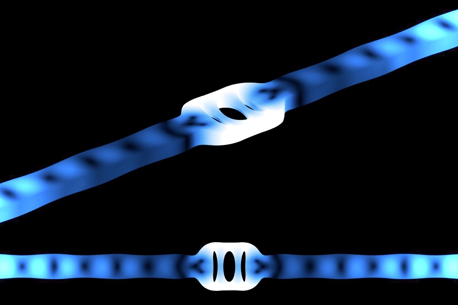
Figure 1: Visualization of a mechanical QNM on a 3-hole optomechanical nanobeam cavity, which will spatially diverge because of teh outgoing boundary conditions.

In most optomechanical mode theories to date, the optomechanical coupling rate $g_{0}$ is rarely taken from a first-principles model, which is in contrast to modal methods in optics where it is more common to adopt an analytical approach based on the optical modes of the structure. Yet there is clearly a need to describe emerging effects such as mode-to-mode transcription and reservoir engineering in terms of the underlying mode properties of the mechanical cavity modes, both in classical and quantum mechanical problems. A recent theory paper introduced the interesting idea of an elastic Purcell factor Schmidt et al. (2018), which like its optical counterpart, describes an enhancement of a dipole emitter (but now a force dipole), in terms of $Q$ and $V_{\rm eff}$; similar to earlier works on optical cavities, the authors used a “normal mode theory,” which is in general incorrect for open cavity modes Kristensen et al. (2012); however, for high $Q$ cavities, the normal mode approach can be a very good approximation, but the theory is still ambiguous. Experimental measurements have also recently been performed on the acoustic Purcell factor Landi et al. (2018), and thus there is clearly a need to develop mode theories for such geometries and emerging material systems beyond optics.

To account for mode dissipation in optical resonators, the modelling of the dominant cavity mode is usually calculated by implementing outgoing boundary conditions (otherwise it has an infinite lifetime). Often this problem is treated with closed boundary conditions or as a Hermitian eigenvalue problem, but this is inconsistent with a finite cavity loss. In fact, it is now known that all open cavity modes yield spatially divergent modes, which are the QNMs described earlier. Figure 1 shows a schematic representation of an elastic QNM from an optomechanical photonic crystal beam (calculated in detail later), and we note that the mode diverges for spatial position far down the open beam. These QNMs have recently proven to be very powerful in photonics design and simulations Kristensen and Hughes (2014); Lasson et al. (2015); Lalanne et al. (2018); Kristensen et al. (2020). For the purpose of field normalization and developing mode theories, both optical and mechanical modes are usually assumed to be lossless and then dissipation is added later through system-bath coupling theory, or phenomenologically; in contrast, the QNM approach includes losses from the beginning since the eigenfrequencies are complex, unlike normal modes. The QNMs also quantify coupling parameters in a more complete way, an example of which has been shown for two coupled QNMs of dielectric-cavity systems KamandarDezfouli et al. (2017), resulting in striking interference effects that demonstrate how the phase of the mode must be maintained.

In this work, we introduce an intuitive and accurate QNM description for mechanical modes $\tilde{\bf q}_{\rm m}$, which have complex eigenfrequencies, $\tilde{\Omega}_{\rm m}=\Omega_{\rm m}-i\gamma_{\rm m}$, and $Q_{\rm m}=\Omega_{\rm m}/2\Gamma_{\rm m}$. For single mode resonators, This QNM formalism allows a rigorous definition of the effective mode volume $V_{\rm eff,m}$ Purcell et al. (1946); Kristensen et al. (2012); Kristensen and Hughes (2014) for mechanical modes Eichenfield et al. (2009b), or, equivalently in mechanics, the effective motional mass $m_{\rm eff,m}=\rho V_{\rm eff,m}$ Pinard et al. (1999); Gillespie and Raab (1995); Eichenfield et al. (2009b), which is more commonly used in the optomechanics literature Kipfstuhl et al. (2014); Li et al. (2015); Zheng et al. (2012); Chan et al. (2012); Kalaee et al. (2016); Djafari-Rouhani et al. (2016). We first present a generalized elastic effective mode volume $\tilde{V}_{\rm eff,m}(\mathbf{r})$ using a QNM normalization, and show the problems with using a normal mode volume $V_{\rm eff}$. We then use this complex, position dependant $\tilde{V}_{\rm eff,m}(\mathbf{r})$ to carry out an analytical Green function expansion Ge et al. (2014), which can be used to quickly solve a wide range of force-displacement problems in an analogous way to how the photon Green function is being used to carry out light-matter investigations in optics Yao et al. (2010). Then, using the case of two coupled modes, we demonstrate the accuracy of the QNM theory in explaining complex Fano resonances, and demonstrate the clear failure of the usual normal mode theory for these acoustic modes.

A Fano resonance is a well-known scattering phenomenon that results in asymmetric spectral lineshapes. They have been shown to exist in various physical systems, finding applications in photonics Limonov et al. (2017), plasmonic metamaterials Khanikaev et al. (2013); Luk’yanchuk et al. (2010), and optomechanics Qu and Agarwal (2013); Abbas et al. (2019). In optics, systems that exhibit these phase-dependant interference effects may provide new methods of manipulating light propagation. Applications include sensing, lasing, and optical switching Heuck et al. (2013); Luk’yanchuk et al. (2013); Chen et al. (2015); Limonov et al. (2017). Experimental evidence of Fano resonances in coupled nanomechanical resonators has also been demonstrated in Stassi et al. (2017). Fano resonance phenomena in optomechanical systems can potentially be used for processing classical and quantum information, where the hybridized mechanical modes exhibiting Fano excitation lineshapes allow for an on-chip platform for storage and photonic-phononic quantum state transfer, demonstrated experimentally by studying the coherent mixing of mechanical excitations within optomechanical cavities Lin et al. (2010). Often Fano-resonances are associated with the interference between a bound resonance and a continuum, such as through a cavity and waveguide, but two coupled resonators can also yield a Fano resonance. For example, hybrid plasmonic-dielectric systems cam show a significant Fano resonance Barth et al. (2010); Doeleman et al. (2016); KamandarDezfouli et al. (2017), which can be explained using optical QNM theory KamandarDezfouli et al. (2017) with only two coupled QNMs, and also gives rise to new regimes in quantum optics Franke et al. (2019, 2020). The investigation of coupled mechanical modes in optomechanical systems often rely on the power spectral density measurements with finite element methods typically being used for only initial rudimentary descriptions, so there is clearly motivation in being able to describe such effects as the level of an intuitive and accurate mechanical mode theory.

The rest of our paper is organized as follows: In Sec. II, we present the main theory details and important formulas, introducing the elastic wave equations, QNMs, generalized effective mode volume, and elastic Purcell formula. In Sec. III, we present numerical calculations for a fully 3D optomechanical beam, first for a single QNM design, and then for coupled QNMs that show a striking Fano resonance. In both cases, we highlight the failure of using a normal mode theory, which is shown to be drastic in the case of two coupled modes. Finally, in Sec. IV, we present closing discussions and our main conclusions.

II Theory

II.1 Wave equations, normal modes, quasinormal modes and Green functions

Vibrational modes of solids can be calculated using the linear theory of elasticity Slaughter (2002), where one assumes infinitesimal deformations and stress forces that do not result in “yielding” (deformation point of no elastic return).

We first express Newton’s second law in terms of the displacement vector $\mathbf{u}({\bf r},t)$:

$${\bm{\nabla}}\cdot{\bm{\sigma}}(\mathbf{r},t)-\rho(\mathbf{r})\ddot{\mathbf{u}}(\mathbf{r},t)=-\mathbf{f}(\mathbf{r},t),$$ (2)

where $\rho$ is the mass per unit volume, $\mathbf{f}(\mathbf{r},t)$ is the force vector or force per unit volume, and ${\bm{\sigma}}$ is the stress tensor. Assuming a harmonic solution of the form, ${\bf u}({\bf r},t)=\mathbf{u}({\bf r},\Omega)e^{-i\Omega t}$, and in the absence of a force excitation, we obtain the wave equation in an analogous form to the Helmholtz equation in optics:

$${\bm{\nabla}}\cdot{\bm{\sigma}}(\mathbf{r},\Omega)+\Omega^{2}\rho(\mathbf{r})\mathbf{{u}}(\mathbf{r},\Omega)=0.$$ (3)

The stress tensor can be expressed as Snieder (2002)

$${\sigma_{ij}(\mathbf{r},\Omega)}=c_{ijkl}\partial_{k}u_{l}(\mathbf{r},\Omega),$$ (4)

where $c_{ijkl}$ is the fourth-order elasticity tensor (where one sums over repeated indices as with Einstein summation convention), and $\partial_{k}\equiv\frac{\partial}{\partial x_{k}}$ is the partial derivative with respect to the $x_{k}$ direction. Subjecting Eq. (3) to periodic or hard-wall boundary conditions would yield “normal modes” $\mathbf{q}_{{\rm m}}$ from the following eigenvalue problem:

$$\rho(\mathbf{r}){\Omega}_{\rm m}^{2}{q}_{{\rm m}\it{i}}(\mathbf{r}){+}{\partial}_{j}(c_{ijkl}\partial_{k}{q}_{{\rm m}\it{l}}(\mathbf{r}))=0,$$ (5)

where the eigenfrequencies are real and do not account for dissipation.

It is also useful to define the corresponding Green function ${\mathbf{G}}$, obtained from Snieder (2002):

$$\partial_{j}(c_{ijkl}\partial_{k}G_{ln}(\mathbf{r},\mathbf{r^{\prime}};\Omega))\\ +\rho(\mathbf{r})\Omega^{2}G_{in}(\mathbf{r},\mathbf{r^{\prime}};\Omega)=-\delta_{in}\delta(\mathbf{r}-\mathbf{r^{\prime}}),$$ (6)

where the $i$th component of a unit force in the $n$ direction at location ${\bf r}^{\prime}$ is given by $\delta_{in}\delta({\bm{r}}-{\bm{r}}^{\prime})$. The displacement can be written in terms of ${\mathbf{G}}$ as Snieder (2002):

$${u_{i}}(\mathbf{r})=\int_{V}{G_{in}}(\mathbf{r},\mathbf{r^{\prime}})\cdot{f_{n}}(\mathbf{r})d{\bf r^{\prime}}\\ +\oint_{S}\{G_{in}(\mathbf{r},\mathbf{r^{\prime}})\hat{\rm s}_{j}c_{njkl}\partial_{k}^{\prime}u_{l}(\mathbf{r^{\prime}})\\ -u_{n}(\mathbf{r^{\prime}})\hat{\rm s}_{j}c_{njkl}\partial_{k}^{\prime}G_{il}(\mathbf{r,r^{\prime}})\}d{\bf r^{\prime}},$$ (7)

where $\hat{\rm s}_{j}$ is the normal vector of $S$, the surface forming the outer boundary of the elastic body. For an elastic body surrounded by empty space, the second term vanishes as there is no stress at the surface. In the case of a point force excitation, $\mathbf{f}(\mathbf{r},t)=\mathbf{f}_{\rm d}\delta({\bm{r}}-{\bm{r}}_{0})\delta(t)$, then

$${\mathbf{u}}(\mathbf{r},\Omega)=\mathbf{G}(\mathbf{r},\mathbf{r}_{0};\Omega)\cdot{\bf f}_{\rm d}(\mathbf{r}_{0}),$$ (8)

where ${\bf f}_{\rm d}$ is a point force at position $\mathbf{r}_{0}$.

Using the completeness relation for normal modes,

$${\mathbf{I}}\delta(\mathbf{r}-\mathbf{r^{\prime}})=\sum_{{\rm m}=1,2,\cdots}\rho(\mathbf{r}){\mathbf{q}}_{\rm m}(\mathbf{r}){\mathbf{q}}^{\dagger}_{\rm m}(\mathbf{r^{\prime}}),$$ (9)

(where $\mathbf{I}$ is a unit dyadic of a 3x3 matrix, the dagger denotes the complex conjugate of the transpose: $\mathbf{q}^{\dagger}=(\mathbf{q}^{T})^{*}$, and ${\rm m}=1,2,\cdots$) the Green function can be obtained from an expansion over the normal modes Snieder (2002)

$${\mathbf{G}}(\mathbf{r},\mathbf{r^{\prime}};\Omega)=\sum_{{\rm m}=1,2,\cdots}\frac{\mathbf{q}_{\rm m}(\mathbf{r})\mathbf{q}_{\rm m}^{\dagger}(\mathbf{r^{\prime}})}{\Omega^{2}_{\rm m}-\Omega^{2}}.$$ (10)

For problems in cavity physics with a few modes of interest, the above theory is not that useful or practical, since one needs a continuum of modes. Instead, similar to open-cavity problems in optics, one desires to describe the main physics in terms of just a few discrete resonator modes. In an elastic resonator medium with open boundary conditions, the resonator modes $\tilde{\mathbf{q}}_{\rm m}$ are obtained from:

$$\rho(\mathbf{r})\tilde{\Omega}_{\rm m}^{2}\tilde{q}_{{\rm m}\it{i}}(\mathbf{r}){+}{\partial}_{j}(c_{ijkl}\partial_{k}\tilde{q}_{{\rm m}\it{l}}(\mathbf{r}))=0,$$ (11)

where $\tilde{\Omega}_{\mathbf{{\rm m}}}$ is the complex eigenfrequency and $\tilde{\bf q}_{\rm m}({\bf r})$ are the QNMs.

We can now exploit techniques that have been recently developed for obtaining QNMs and QNM Green functions in optics Kristensen and Hughes (2014); Lee et al. (1999); Lalanne et al. (2018); Kristensen et al. (2020). Using a modified completeness relation for QNMs Lee et al. (1999)

$${\mathbf{I}}\delta(\mathbf{r}-\mathbf{r^{\prime}})=\sum_{{\rm m}=\pm 1,\pm 2,\cdots}\frac{1}{2}\rho(\mathbf{r})\tilde{\mathbf{q}}_{\rm m}(\mathbf{r}){[}\tilde{\mathbf{q}}_{\rm m}(\mathbf{r^{\prime}}){]^{T}},$$ (12)

where now ${\rm m}=\pm 1,\pm 2,\cdots$, superscript $T$ denotes the transpose, and we assume this condition is satisfied for spatial positions within or near the cavity Kristensen and Hughes (2014); Lalanne et al. (2018). Note that the tensor product in Eq. 12 is also frequently written as $\tilde{\mathbf{q}}_{\rm m}(\mathbf{r})\otimes\tilde{\mathbf{q}}_{\rm m}(\mathbf{r^{\prime}})$. We can thus expand ${\mathbf{G}}$ in terms of QNMs, through (alternative expansion forms, for optical QNMs, are discussed in Kristensen et al. (2020))

$${\mathbf{G}}(\mathbf{r},\mathbf{r^{\prime}};\Omega)=\sum_{{\rm m}=\pm 1,\pm 2,\cdots}\frac{\tilde{\mathbf{q}}_{\rm m}(\mathbf{r}){[}\tilde{\mathbf{q}}_{\rm m}(\mathbf{r^{\prime}}){]^{T}}}{2{\Omega}(\tilde{\Omega}_{\rm m}-{\Omega})}.$$ (13)

To have quantities that better relate to a mode volume in optics, which is also a key quantity in Purcell’s formula, we next define an alternative QNM through

$$\tilde{\mathbf{Q}}_{{\rm m}}(\mathbf{r})=\sqrt{\rho({\bf r})}\,\tilde{\mathbf{q}}_{{\rm m}}(\mathbf{r}),$$ (14)

so that $\tilde{\mathbf{Q}}^{2}_{{\rm m}}$ has units of inverse volume. There have been various approaches to obtain normalized QNMs in optics Kristensen et al. (2012); Kristensen and Hughes (2014); Kristensen et al. (2015); Sauvan et al. (2013); Lalanne et al. (2018); Muljarov et al. (2010); Bai et al. (2013); Zschiedrich et al. (2018), and in this work we use

$$\langle\langle{\tilde{\mathbf{Q}}}_{{\rm m}}|{\tilde{\mathbf{Q}}_{{\rm n}}}\rangle\rangle=\lim_{V\to\infty}\int_{V}\tilde{\mathbf{Q}}_{{\rm m}}(\mathbf{r})\cdot\tilde{\mathbf{Q}}_{{\rm n}}(\mathbf{r})d\mathbf{r}\\ +i\frac{\displaystyle{\varv}_{\rm s}^{\rm b}}{\displaystyle 4\pi\tilde{\Omega}_{\rm m}}\int_{{A}}\tilde{\mathbf{Q}}_{{\rm m}}(\mathbf{r})\cdot\tilde{\mathbf{Q}}_{{\rm n}}(\mathbf{r})d\mathbf{r}=\delta_{{\rm m},{\rm n}},$$ (15)

which is analogous to the optical QNM normalization introduced by Lai et al. Lai et al. (1990), and was used to introduce the idea of a “generalized mode volume” with optical cavities Kristensen et al. (2012). Compared to its optical counterpart, we note the following substitutions: (i) speed of light, $c$ $\rightarrow$ shear speed of sound in bulk material ${\varv}_{\rm s}^{\rm b}$ (as we are only considering transverse modes); and (ii), refractive index $n_{\rm B}$ $\rightarrow$ material density $\rho$. Note that Eq. (15) needs a careful regularization if evaluated over a large simulation volume Kristensen et al. (2015).

In terms of these new elastic QNMs, the Green function expansion can now be written as

$${\mathbf{G}}(\mathbf{r},\mathbf{r^{\prime}};\Omega)=\sum_{{\rm m}=\pm 1,\pm 2,\cdots}\frac{\tilde{\mathbf{Q}}_{\rm m}(\mathbf{r}){[}\tilde{\mathbf{Q}}_{\rm m}(\mathbf{r^{\prime}}){]^{T}}}{\rho(\mathbf{r})2{\Omega}(\tilde{\Omega}_{\rm m}-{\Omega})},$$ (16)

where we now only need to perform a sum over just a few dominate modes of interest. We stress that not only does this theory give a rigorous definition of Purcell’s formula (as we show below), but it fully accounts for phase effects and non-Lorentzian features from the complex QNMs.

II.2 Complex mode volumes and the elastic Purcell formula in terms of QNMs

The common approach to obtaining mode volumes in the literature Schmidt et al. (2018); Eichenfield et al. (2009b); Kipfstuhl et al. (2014); Djafari-Rouhani et al. (2016), is to define the effective mode volume, in the present case for acoustic modes, using a normal mode normalization:

$$V_{{\rm eff},{\rm m}}^{\rm NM}=\frac{\displaystyle\int d\mathbf{r}|{\tilde{\mathbf{Q}}_{{\rm m}}}(\mathbf{r})|^{2}}{\displaystyle\rm{max}[|{\tilde{\mathbf{Q}}_{{\rm m}}}(\mathbf{r})|^{2}]},$$ (17)

where $\mathbf{\tilde{Q}}_{\rm m}$ is actually the QNM spatial profile (solution with outgoing boundary conditions), but without the normalization of Eq. (15). However, Eq (17) is problematic as the value diverges as a function of space for any dissipative modes (unless they are lossless). In essence it uses a theory for the normal modes ${\bf Q}_{\rm m}$, which are solutions to a Hermitian eignevalue, and so it is incorrect to then use a QNM as the mode solution.

To fix this problem, the QNM normalization condition in Eq. (15) allows one to obtain a complex (or generalized) effective mode volume for a mechanical mode:

$${\tilde{V}_{{\rm eff},{\rm m}}(\mathbf{r})}=\frac{1}{\tilde{\mathbf{Q}}^{2}_{{\rm m}}(\mathbf{r})},$$ (18)

where $\tilde{V}_{{\rm eff,m}}=V_{{\rm eff,m}}+iV^{\rm Im}_{{\rm eff,m}}$, for a specific mode ${\rm m}$. Note also that we allow the effective mode volume to be a function of space here as it formally characterises the mode strength squared at those positions, and is not directly related to the integrated mode volume (which diverges). For closed cavities, the field squared happens to be related to the total volume of the mode if evaluated at the field maximum. In QNM theory, the total mode volume is ill defined, as it diverges for any open cavity resonator. Thus one can refer to this quantity as a “localized mode volume,” where the volume is a useful figure of merit for certain applications of interest. As we will show later, the phase of the QNM can have profound consequences, and is essential to the general theory.

As explained in the introduction, this modal Purcell factor theory has been well exploited in optical cavity physics and cavity-QED for decades, and the underlying physical insight in terms of cavity mode properties would be hard to underestimate as a design tool. Thus, here we aim to derive the expression for an elastic Purcell factor, similar to the work of Schmidt et al. Schmidt et al. (2018), but now in terms of the more appropriate QNM Green functions.

The mechanical Purcell factor evaluated of an elastic emitter (coupled to a QNM), ${\bf f}_{\rm{d}}={f}_{\rm{d}}\bf{n}$, oriented along direction ${\bf n}$, at some position $\mathbf{r}_{0}$ and at a frequency $\Omega$ can be written as

$$F_{\rm P}({\bf r}_{0},\Omega)=\frac{P({\bf r}_{0})}{P_{0}({\bf r}_{0})}=\frac{\rm{Im}[{\bf f}_{\rm{d}}^{\dagger}\cdot\mathbf{G}(\mathbf{r}_{0},\mathbf{r}_{0};\Omega)\cdot{\bf f}_{\rm{d}}]}{\rm{Im}[{\bf f}_{\rm{d}}^{\dagger}\cdot\mathbf{G}_{0}(\mathbf{r}_{0},\mathbf{r}_{0};\Omega)\cdot{\bf f}_{\rm{d}}]},$$ (19)

where $\mathbf{G}_{0}$ is the Green function in a homogeneous medium. Note that ${\bf G}_{0}$ includes both transverse and longitudinal modes, whereas the QNM one (${\bf G}$) is for transverse modes only ($\tilde{\Omega}\neq 0$), which completely dominates the response for resonant cavity structures. One can think of Eq. (19) as a generalized enhancement factor or generalized Purcell factor, as no mode expansions have been performed yet (which is necessary to connect to the usual single mode Purcell formula). The terms $P$ and $P_{0}$ are the radiated power from a dipole (at position ${\bf r}_{0}$) in an inhomogeneous and homogeneous medium, respectively. Using an analogous approach to Poynting’s theorem, $P_{0}$ is formally defined from Novotny and Hecht (2006); Schmidt et al. (2018):

$$P_{0}({\bf r}_{0})=\frac{dW({\bf r}_{0})}{dt}=\frac{\Omega}{2}{\rm Im}[{\bf f}_{\rm d}^{*}\cdot{\mathbf{u}}(\mathbf{r}_{0})],$$ (20)

which can be derived analytically for an isotropic medium Schmidt et al. (2018):

$$P_{0}({\bf r}_{0})=\frac{\Omega^{2}|{\bf f}_{\rm{d}}|^{2}\alpha}{12\pi\rho(\mathbf{r}_{0})},$$ (21)

where

$$\alpha=\frac{1}{2}\varv^{-3}_{\rm l}+\varv^{-3}_{\rm s},$$ (22)

in which $\varv_{\rm l}$ and $\varv_{\rm s}$ are the scalar longitudinal and shear speed of sound in the material, respectively. We can therefore write Eq. (19) as

$$F_{\rm p}({\bf r}_{0},\Omega)=\eta_{\bf n}\frac{6\pi\rho(\mathbf{r}_{0})\rm{Im}[{\bf f}_{\rm{d}}^{\dagger}\cdot\mathbf{G}(\mathbf{r}_{0},\mathbf{r}_{0};\Omega)\cdot{\bf f}_{\rm{d}}]}{\Omega|{f}_{\rm{d}}|^{2}\alpha}.$$ (23)

where we have introduced a numerically determined constant $\eta_{\bf n}$ (which depends on the dipole direction in general) to account for elastic anisotropy of the medium; for relatively isotropic crystals, $\eta_{\bf n}\approx 1$.

The medium Green function can now be used with our generalized effective mode volume $\tilde{V}_{\rm eff}$ and Eq. (23) for a multi-mode approximation of a cavity decay rate enhancement, and for various other problems in optomechanics. We thus obtain the multi-QNM Green function expansion evaluated at a point $\mathbf{r}_{0}$ within the resonator:

$$F_{\rm p}({\bf r}_{0},\Omega)=\eta_{\bf n}\frac{6\pi\rho(\mathbf{r}_{0})}{\Omega|f_{d}|^{2}{\alpha}}\times\\ \rm{Im}\left[{\bf f}_{\rm{d}}^{\dagger}\cdot\sum_{{\rm m}}\frac{\tilde{\mathbf{Q}}_{\rm m}(\mathbf{r}_{0}){[}\tilde{\mathbf{Q}}_{\rm m}(\mathbf{r}_{0}){]^{T}}}{\rho(\mathbf{r}_{0})2{\Omega}(\tilde{\Omega}_{\rm m}-{\Omega})}\cdot{\bf f}_{\rm{d}}\right].$$ (24)

For a slightly more familiar form, we can write this in terms of the (complex) effective mode volume as:

$$F_{\rm p}({\bf r}_{0},\Omega)=\eta_{\bf n}\frac{6\pi\rho(\mathbf{r}_{0})}{\Omega{\alpha}}\times\\ \rm{Im}\left[\sum_{{\rm m}}\frac{1}{\rho(\mathbf{r}_{0})2{\Omega}(\tilde{\Omega}_{\rm m}-{\Omega})\tilde{V}_{{\rm m},{\rm eff}}(\mathbf{r}_{0})}\right],$$ (25)

where we have assumed that the force direction is along the dominant polarization component of the mode, which is the usual assumption in Purcell’s formula.

Finally, using Eq. (23), we have the enhanced emission rate for a single QNM:

$$F_{\rm p}({\bf r}_{0})=\eta_{\bf n}\frac{6\pi Q_{{\rm m}}}{\Omega^{3}_{{\rm m}}{\alpha}V_{{\rm eff},{\rm m}}({\bf r}_{0})},$$ (26)

in which we assume that the Green function’s response is dominated by a single mode, and the response is on-resonance ($\Omega=\Omega_{\rm m}$). Equation (26) is the elastic Purcell factor evaluated at the resonant mode $\Omega_{\rm m}$ at the source point, whereas Eq. (25) is generalized for various positions and frequencies. Our expression is consistent with the expression recently presented by Schmidt et al. (2018), but with a “corrected” and generalized effective mode volume, consistent for an open cavity mode with complex eigenfrequencies and an unconjugated norm. Note also that our Green function explicitly includes the QNM phase, which we show below is essential for describing the response function of several QNMs, which can yield highly non-Lorentzian lineshapes. For background media that are relatively isotopic, $\eta_{\bf n}\approx 1$ (as we find for crystalline Si below), and one can simply drop this factor from the Purcell formula and main equations.

III Numerical Results

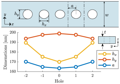
Figure 2: Design specifications of the optomechanical nanobeam cavity, with unit cell parameters $a$, $h_{x}$, and $h_{y}$. Dimensions: $w=0.53\,\rm{\mu}m$ and $t=0.22\,\rm{\mu}m$. The beam is simulated to be infinitely long using perfectly matched layers. The origin of this coordinate system, $(x,y,z)=(0,0,0)$, is placed at the center of hole-0 at half beam thickness. The 3-hole cavity design uses the holes: -1, 0, and 1.

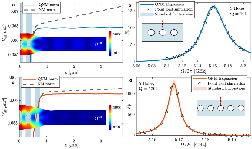
Figure 3: a,c Real part of the complex effective mode volume $V_{{\rm eff,m}}$ using the QNM mode normalization from Eq. (15) (solid line) and normal mode (‘NM’) normalization from Eq. (17) (dashed) for a 3-hole and 5-hole nanobeam OMC cavity, respectively, evaluated at ${\bf r}_{0}=(0.0,235.5,0.0)$ nm). Blue shading indicates hole positions with respect to the shown mode profile, which is symmetrical about the $y$-axis at the cavity center. b,d Enhancement rate $F_{\rm P}$ calculated using the Green function expansion (Eq. (25)) (with an isotropic material approximation $\eta_{\bf n}=1$) for the QNMs of interest (solid line). Numerical exact (e.g., with no approximations) Purcell factor Eq. (27)) obtained from averaged numerical point load simulation from COMSOL (see text). Shaded lines show plus/minus one standard deviation of the numerical solution with mesh sensitivity included.

III.1 Mechanical mode effective mode volumes and Purcell factors

We now corroborate our mechanical QNM theory against rigorous numerical calculations obtained for fully three-dimensional mechanical cavities of practical interest in optomechanics. Naturally, the above theory can easily be applied to two dimensional and one dimensional systems as well, with appropriate changes for the background Green functions Kristensen et al. (2012, 2020).

In this work, we are interested in modelling optomechanical crystal (OMC) cavities on dielectric nanobeams. We consider the impressive nanobeam structure developed by Painter and collaborators Chan et al. (2012), consisting of periodic holes with a lattice taper region, in which the hole spacing and size changes. The taper region causes a Fabry-Pérot like effect, resulting in spatially overlapping localized optical and mechanical modes. We adapt the original structure to produce higher loss QNMs by using only a small number of holes to form the OMC cavity. This is so that we may test our QNM normalization at low-$Q$, where the normal mode approximation breaks down more dramatically.

The nanobeam is modeled as anisotropic silicon in free space with elasticity matrix elements $(C_{11},C_{12},C_{44})=(166,64,80)$ GPa. We consider two OMC cavities, one consisting of 3 holes (3H), and one of 5 holes (5H). Cavity design parameters are specified in Fig. 2 along with the beam dimensions. Each cavity design exhibits single mode behaviour over the frequency ranges shown in Fig. 3. We conduct our numerical investigations using the finite element analysis (FEM) commercial software, COMSOL. The beam is simulated to be infinitely long by implementing perfectly matched layers (PMLs), which simulate outgoing boundary conditions.

Employing the eigenfrequency solver, we obtain the dominant QNMs of interest for each cavity at $\tilde{\Omega}^{3\rm{H}}/2\pi=5.160-i0.016$ GHz and $\tilde{\Omega}^{5\rm{H}}/2\pi=5.168-i0.002$ GHz. The spatial profile of each mode is shown in Figs. 3a and 3c. We evaluate the effective mode volume of the 3H and 5H QNMs at ${\bf r}_{0}=(0.0,235.5,0.0)$ nm (where there is strong localization). Using Equation (18) with the QNM normalization in Eq (15), the real part of the generalized effective mode volume $\tilde{V}_{\rm eff}$ is plotted as a function of simulation size against the more commonly used normal mode $V_{\rm eff}^{\rm NM}$ (Note that the surface term in Eq (15) is only applied outside of the hole region as it assumes a constant outgoing medium). The normal mode normalization in Eq (17) assumes that the mode is localized in space. Consequently, when applied to any cavity mode with finite leakage, $V_{\rm eff}^{\rm NM}$ will diverge exponentially when integrated over all space. For less leaky cavities, this divergence is initially quite slow for a small simulation size, whereas the effect is more dramatic for low-$Q$ modes. The QNM normalization, in contrast, converges as the calculation domain is increased, though may eventually oscillate around the correct value and require regularization Kristensen et al. (2012, 2015). Using a sufficient calculation domain size, we obtain $\tilde{V}_{\rm eff}^{3{\rm H}}({\bf r}_{0})=0.06487+0.00943i$ $\mu$m³ and $\tilde{V}_{\rm eff}^{5{\rm H}}({\bf r}_{0})=0.06155-0.00355i$ $\mu$m³.

We now make use of the generalized effective mode volume to investigate the elastic Purcell effect. The numerically exact Purcell factor is calculated from

$$F_{\rm P}^{\rm exact}({\bf r}_{0})=\frac{P_{\rm inhom}({\bf r}_{0})}{P_{0}},$$ (27)

where $P_{\rm inhom}$ is the power emission from a point load in the inhomogeneous structure (in this case the beam cavity), and $P_{0}$ from a homogeneous sample. We employ the frequency domain solver in COMSOL to obtain full numerical calculations (plotted in Figure 3 b,d). See Appendix C for details on the numerical simulations.

Figures 3 b,d show the semi-analytical enhancement rate $F_{\rm P}(\Omega)$ calculated using Eq. (25) with $\tilde{V}_{\rm eff}^{3{\rm H}}({\bf r}_{0})$ and $\tilde{V}_{\rm eff}^{5{\rm H}}({\bf r}_{0})$ for the dominant QNM modes of interest, $\tilde{\Omega}^{3\rm{H}}$ and $\tilde{\Omega}^{5\rm{H}}$, respectively. In order to determine $\eta_{\bf n}$, anisotropic material parameters are applied to a numerical model of a homogeneous sample in which the simulation parameters produce a power spectrum agreeing with the analytical expression in Eq. (21) when isotropic material parameters are used. For our case, we use (and have verified) the isotropic approximation of $\eta_{\bf n}=P_{0}^{\rm iso}(\Omega)/P_{0}^{\rm aniso}(\Omega)\approx 1$, where $P_{0}^{\rm iso}$ and $P_{0}^{\rm aniso}$ are the radiated power from a point load in an isotropic and anisotropic homogeneous medium, respectively. Also plotted in Fig. 3 b,d is the numerically obtained Purcell factor $F_{\rm P}^{\rm exact}$ calculated from fully three-dimensional frequency domain point load simulations. To account for numerical fluctuations (see Appendix C), the average of multiple simulations were conducted in which the mesh parameters are slightly changed. Within this fluctuation, we find excellent agreement between the full numerical simulations and the semi-analytical Green function expansion, with the single-mode approximation being sufficient in describing the dominant resonance response of the system. It is worth mentioning that the modal description provides the enhancement of an emitter at any location and frequency given a sufficient number of QNMs (and often just one QNM) which can be calculated in minutes on a single computer. In contrast, normally one must perform a frequency domain calculation for one frequency at a single point load position, which can take anywhere from hours to days for a sufficient spectrum.

III.2 Coupled mechanical quasinormal modes

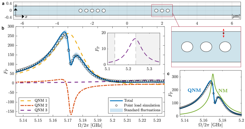
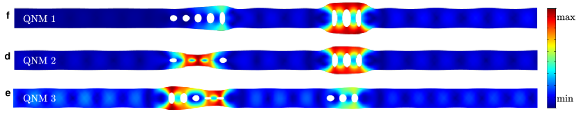
Figure 4: a Optomechanical crystal beam geometry, consisting of a 3-hole and a 5-hole cavity seperated by 4 $\mu$m. Zoom-in box shows the simulated point load orientation (aligned with the breathing mode’s dominant polarization) and position at ${\bf r}_{0}=(2300.0,235.0,0.0)$ nm. b Purcell simulation with a 3-mode approximation of the total decay rate at the same ${\bf r}_{0}$ (solid line) calculated using Eq. 25 (using an isotropic material approximation $\eta_{\bf n}=1$) . Contributions from each individual modes are shown with dashed lines. Inset shows a clearer view of QNM 3, where un-shaded region indicates the frequency range of main plot. Circles show averaged numerical FEM calculations of $F_{\rm P}^{\rm exact}$ (Eq. 27), with the shaded region showing +/- one standard deviation. c Total decay rate calculated using the normal mode approximation (where the effective mode volume is obtained from Eq. 17), compared with FEM numerical solution. d,e,f Mode profiles of QNM 1 ($\tilde{\Omega}_{\rm 1}/2\pi=5.172-i0.012$ GHz), QNM 2 ($\tilde{\Omega}_{\rm 2}/2\pi=5.171-i0.002$), and QNM 3 ($\tilde{\Omega}_{\rm 3}/2\pi=5.232-i0.041$ GHz), respectively. Color bar indicates the minimum and maximum displacement relative to each individual mode. Note that these modes are not the original modes, but hybrid modes including the dissipation-induced coupling.

Having demonstrated the validity of the generalized effective mode volume with the single mode approximation, we now consider coupled QNMs. The optomechanical cavity used above can support both high-$Q$ and low-$Q$ modes, depending on the design and quantity of holes used. We consider an OMC nanobeam structure with two cavities, one designed for relatively high-Q modes (5H), and one for low-Q modes (3H).

Figure 4a shows the nanobeam structure, using the same cavity design parameters outlined in Fig. 2 and a separation of 4 $\mu$m between the two cavities. We look at two resonant QNMs of interest that are close in frequency with spectral overlap. The first of which, QNM 1 with eigenfrequency $\tilde{\Omega}_{\rm 1}/2\pi=5.172-i0.012$ GHz ($Q_{1}=216$), is dominated by the 3-hole cavity (mode profile is shown in Figure 4d). The second, QNM 2 with $\tilde{\Omega}_{\rm 2}/2\pi=5.171-i0.002$ GHz ($Q_{2}=1293$), is dominated by the 5-hole cavity (Fig. 4e).

We evaluate the the generalized effective mode volume near the antinode of the 3-hole cavity at ${\bf r}_{0}=(2300.0,235.0,0.0)$ nm, and use the multi-QNM Green function expansion to describe the frequency response at this position in Fig. 4b. Here we seem the hybridization of the individual modes studied earlier ($\tilde{\Omega}^{3\rm{H}}$ and $\tilde{\Omega}^{5\rm{H}}$), where QNM 2 exhibits a Fano-resonance that results in an interference effect in the total decay rate. Note that we have used a 3rd mode in our approximation, QNM 3 ($\tilde{\Omega}_{\rm 3}/2\pi=5.232-i0.041$ GHz, $\tilde{V}_{\rm eff,3}({\bf r}_{0})=-0.280-0.006$ $\mu$m³), to allow for a total decay rate that is positive and well behaved in a large frequency range of interest (while the total decay rate is physically meaningful, contributions from individual modes may not always be); note, however, this mode has negligible contribution to the main dominant response (between 5.15 and 5.19 GHz), and the two-QNM description sufficiently describes the system response. Indeed, we once again have excellent agreement with FEM point load simulations (see Fig. 4b).

For a more intuitive understanding of the role of the mode phase $\phi_{\rm m}{(\bf r_{0})=\rm arg(\tilde{\bf Q}(\bf r_{0}))}$, with two QNMs, we can write Eq. (25) in terms of the two dominant QNMs (QNM 1 and QNM 2) as:

$$F_{\rm p}({\bf r}_{0},\Omega)|_{\rm cos+sin}=\frac{3\pi^{2}\eta_{\bf n}}{\Omega^{2}\alpha}\times$$

$$\left(\left[\cos 2\phi_{1}({\bf r}_{0})+\frac{\Omega_{1}-\Omega}{\gamma_{1}}\sin 2\phi_{1}({\bf r}_{0})\right]|{\tilde{\bf Q}_{1}}({\bf r}_{0})|^{2}\,L_{1}(\Omega)\right.$$

$$+\left.\left[\cos 2\phi_{2}({\bf r}_{0})+\frac{\Omega_{2}-\Omega}{\gamma_{2}}\sin 2\phi_{2}({\bf r}_{0})\right]|{\tilde{\bf Q}_{2}}({\bf r}_{0})|^{2}\,L_{2}(\Omega)\right),$$ (28)

where we use the normalized Lorentzian function,

$$L_{\rm m}(\Omega)=\frac{\gamma_{\rm m}/\pi}{(\Omega_{\rm m}-\Omega)^{2}+\gamma_{\rm m}^{2}},$$ (29)

and we assume the force dipole is projected along the dominant field direction, namely $|\tilde{\bf Q}|^{2}=|{\bf\tilde{Q}\cdot{\bf n}}|^{2}$, though this can easily be generalized. To better clarify the underlying physics of the various phase terms, we also define two other functions, one that neglects the $\sin$ contributions:

$$F_{\rm p}({\bf r}_{0},\Omega)|_{\rm\cos} =\frac{3\pi^{2}\eta_{\bf n}}{\Omega^{2}\alpha}\times$$

$$\big{(}\cos 2\phi_{1}({\bf r}_{0})|{\tilde{\bf Q}_{1}}({\bf r}_{0})|^{2}\,L_{1}(\Omega)$$

$$+ \cos 2\phi_{2}({\bf r}_{0})|{\tilde{\bf Q}_{2}}({\bf r}_{0})|^{2}\,L_{2}(\Omega)\big{)},$$ (30)

and one that neglects the phase completely:

$$F_{\rm p}({\bf r}_{0},\Omega)|_{\rm abs}=$$

$$\ \ \ \frac{3\pi^{2}\eta_{\bf n}}{\Omega^{2}\alpha}\left(|{\tilde{\bf Q}_{1}}({\bf r}_{0})|^{2}\,L_{1}(\Omega)+|{\tilde{\bf Q}_{2}}({\bf r}_{0})|^{2}\,L_{2}(\Omega)\right).$$ (31)

All three agree (Eqs. (III.2),(III.2), (III.2)) only when $\cos(2\phi_{1})=\cos(2\phi_{2})=1$, and $\sin(2\phi_{1})=\sin(2\phi_{2})=0$. Note also that Eq. (III.2) has the same form as a normal mode solution, though its effective mode volume is different, and the later will in general be overstated (yielding a smaller Purcell factor value).

For our numerical example, the QNM phase values at the point of interest are $2\phi_{1}(\mathbf{r}_{0})=0.3204$ and $2\phi_{2}(\mathbf{r}_{0})=2.4643$ for QNM 1 and QNM 2, respectively. While the QNM 1 phase shift $\phi_{1}$ is relatively small, the near $180^{o}$ phase shift of ${\bf\tilde{Q}_{2}}^{2}({\bf r}_{0})$ results in the negative contribution to the overall enhancement. From these phase values, the cosine values are $\cos(2\phi_{1})\approx 0.95$ and $\cos(2\phi_{1})\approx-0.7$, so the latter will contribute as a negative Lorentzian lineshape. Figure 2 shows the Purcell factor predictions from Eqs. (III.2), (III.2), and (III.2), which clearly demonstrates the role of the phase terms. We can see that neglecting the phase of the mode fails entirely in describing the interference effect (Figure 5a). Considering only the cosine terms still provides a negative contribution from QNM 2 (this is equivalent to only using the real part of $\tilde{V}_{\rm eff,1}$), however, the asymmetry of the lineshape requires the full phase. In fact, the sin terms are $\sin(2\phi_{1})\approx 0.31$ and $\sin(2\phi_{1})\approx 0.36$, which are significant and certainly cannot be ignored in general. Indeed, the pronounced Fano feature can only be correctly described when the complete phase is used (see Fig. 5b).

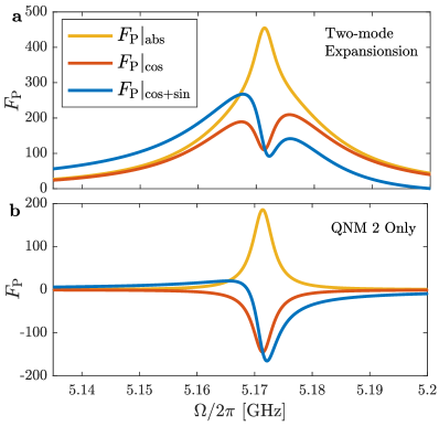
Figure 5: Two QNM expansion (a) and single mode expansion of QNM 2 (b) using all phase terms (Eq. (III.2)), the cos term only (Eq. (III.2), and without any phase dependence (Eq. (III.2)).

Equation (III.2) provides a clear understanding of phase interactions between coupled modes. However, rather than work with the complex phases, it can be convenient to work in the complex effective mode volume picture, i.e Eq. (25), which is in the spirit of Purcell’s formula. A simple way to do this is to write Eq. (III.2) in terms of the real and imaginary parts of the generalized effective mode volume:

$$F_{\rm p}({\bf r}_{0},\Omega)\approx\frac{3\pi^{2}\eta_{\bf n}}{\Omega^{2}\alpha}\times$$

$$\left(\left[{\rm Re}\left(\frac{1}{\tilde{V}_{\rm eff,1}({\bf r}_{0})}\right)+\frac{\Omega_{1}-\Omega}{\gamma_{1}}{\rm Im}\left(\frac{1}{\tilde{V}_{\rm eff,1}({\bf r}_{0})}\right)\right]L_{1}(\Omega)\right.$$

$$+\left.\left[{\rm Re}\left(\frac{1}{\tilde{V}_{\rm eff,2}({\bf r}_{0})}\right)+\frac{\Omega_{2}-\Omega}{\gamma_{1}}{\rm Im}\left(\frac{1}{\tilde{V}_{\rm eff,2}({\bf r}_{0})}\right)\right]L_{2}(\Omega)\right),$$ (32)

where we have effectively replaced the sin and cos terms, as well as $|\tilde{\bf Q}_{\rm m}|^{2}$, with the real and imaginary parts of $1/\tilde{V}_{{\rm eff},{\rm m}}$. It is now easier to see that the normal mode solution using the entirely real $V_{\rm eff,m}^{\rm NM}$ Schmidt et al. (2018) will always be a simple sum of two Lorentzians:

$$F_{\rm p}^{\rm NM}({\bf r}_{0},\Omega) \approx\frac{3\pi^{2}\eta_{\bf n}}{\Omega^{2}\alpha}\left(\frac{L_{1}(\Omega)}{V_{\rm eff,1}^{\rm NM}({\bf r}_{0})}+\frac{L_{2}(\Omega)}{V_{\rm eff,2}^{\rm NM}({\bf r}_{0})}\right),$$ (33)

as plotted in Fig. 4c, which shows a drastic failure of the normal mode theory. Note that Eq. (33) for a single mode is equivalent to the one in Ref. Schmidt et al. (2018).

The calculated generalized effective mode volumes of the QNMs of are interest are $\tilde{V}_{\rm eff,1}({\bf r}_{0})=0.058-0.019i$ $\mu$m³ and $\tilde{V}_{\rm eff,2}({\bf r}_{0})=-0.399-0.321i$ $\mu$m³ for QNM 1 and QNM 2, respectively. The negative nature of $\tilde{V}_{\rm eff}$ at ${\bf r}_{0}$ is simply a result of the phase shift caused by the interaction between the two cavity resonances. This is also seen with QNMs in optics Lasson et al. (2015); KamandarDezfouli et al. (2017), where the QNM phase causes the Fano-like resonance. Using quantized QNMs in quantum optics gives essentially the same result as classical QNM theory in the bad cavity limit (within numerical precision), but where the interpretation is now through off-diagonal mode coupling Franke et al. (2019); here the dissipation-induced interference cannot be explained by normal mode quantum theories such as the dissipative Jaynes-Cumming model. In this regard, it would be very interesting to develop a quantized QNM theory for mechanical modes as well.

IV Conclusions

We have introduced a QNM formalism for mechanical cavity modes and shown that the commonly used normal mode description is problematic for cavity resonances with finite loss. Instead, we have presented and employed a complex, position dependant effective mode volume for mechanical modes using a QNM normalization which can be used to solve a range of force-displacement problems. For validation of the theory, we carried out an analytical Green function expansion using QNMs with the an elastic Purcell factor expression, and found excellent agreement with rigorous numerical simulations for 3D optomechanical beams.

We then demonstrated the accuracy of the QNM theory in explaining interference effects of coupled cavity modes, and pointed out the drastic failure of the usual normal mode theory. Specifically, we explicitly showed the role of the QNM phase in yielding a Fano-like resonance and explained this analytically and numerically from interference effects that are completely absent in a normal mode theory. This QNM approach should serve as a robust and valuable tool in the understanding and and development of emerging optomechanical technologies.

Appendix A Analysis of quasinormal mode 3

The third mode included in the total decay rate in Fig. 4, ‘QNM 3’, has no qualitative influence on the main Fano feature we are modeling. In essence, it merely produces a small background bump in the total decay rate far in frequency from the hybridized modes of interest. However, without its inclusion we have nonphysical negative enhancement, so it is needed in general to quantitativley connect to the total Purcell factor over a relatively broad frequency range. From our calculations, QNM 3 is likely a modification of a (second) mode that arises in the single cavity 5-hole structure at a slightly higher frequency than the primary mode of interest, $\tilde{\Omega}^{\rm 5H}$.

Figure 6 shows (a) the two-mode approximation of the total decay rate of the single 5-hole cavity nanobeam at ${\bf r}_{0}^{\rm 5H}$, along with (b) the spatial profile of QNM 3. This is the same structure used in Fig. 3c, d, in which we used a one-mode approximation using only the primary mode of interest $\tilde{\Omega}^{5\rm{H}}/2\pi=5.168-i0.002$ GHz. Here we also include the nearest resonant mode at $\tilde{\Omega}_{\rm s}^{5\rm{H}}/2\pi=5.210-i0.051$ GHz. With a quality factor of 53 and $\tilde{V}_{\rm eff}^{5{\rm H},{\rm s}}=0.229-0.124i$ $\mu$m³, its contribution to the total day rate over this frequency range is overshadowed by $\tilde{\Omega}^{\rm 5H}$, showing that the single-mode expansion in Fig. 3d is a sufficient approximation. In addition to having comparable quality factors and relative distances in frequency from $\tilde{\Omega}^{\rm 5H}$ and QNM 2, respectively, $\tilde{\Omega}_{\rm s}^{5\rm{H}}$ and QNM 3 have similar mode profiles at the 5-hole cavity region. Leading us to conclude that QNM 3 is simply $\tilde{\Omega}^{5\rm{H}}/2\pi=5.168-i0.002$ GHz adapted to the addition of the 3-hole cavity on the same beam.

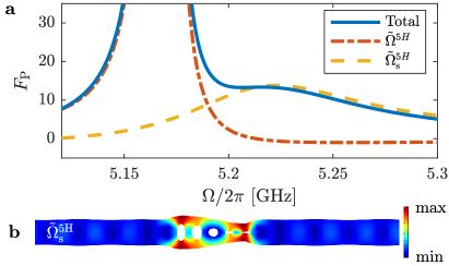
Figure 6: a Two-mode approximation of the total decay rate of the single 5-hole cavity nanobeam at ${\bf r}_{0}=(0.0,235.5,0.0)$ nm calculated using Eq. (25). Dashed lines show the individual mode contributions of the the primary mode $\tilde{\Omega}^{5\rm{H}}$ and secondary mode $\tilde{\Omega}_{\rm s}^{5\rm{H}}$. b Mode profile near the 5 hole cavity of $\tilde{\Omega}_{\rm s}^{5\rm{H}}$ (QNM 3 in the main text).

Appendix B Purcell Factor at different positions

The choice of the evaluation point ${\bf r}_{0}=(0.0,235.5,0.0)$ nm is significant since the QNMs of interest for the single cavity structures are relatively strong at this position. Figure 7 shows the peak Purcell factor of $\tilde{\Omega}^{3\rm{H}}$ and $\tilde{\Omega}^{5\rm{H}}$ modes on two cross sectional lines around this point. The evaluation point for the coupled cavity structure in Figure 4 was chosen simply because it exhibited a pronounced Fano feature. However, for completeness, we also include the total decay rate of the coupled cavity structure evaluated near the 5-hole cavity region in Fig. 8.

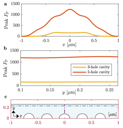
Figure 7: Peak decay rate enhancement of the dominant QNM for the a 3-hole cavity ($\tilde{\Omega}^{3\rm{H}}$) and b 5-hole cavity ($\tilde{\Omega}^{5\rm{H}}$) at a range of $x$ and $y$ evaluation points in the center of the beam ($z=0$ $\mu$m). c shows cross sections at $y=0.2355$ $\mu$m (a, blue dashed) and $x=0$ $\mu$m (b, purple dashed).

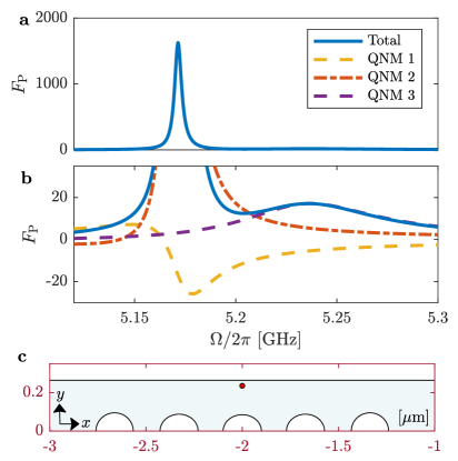
Figure 8: a 3-mode approximation of the total decay rate near the 5-hole cavity region of the coupled cavity structure (${\bf r}_{0}=(-2000.0,235.5,0.0)$ nm). b Zoom-in of a, with contributions from each individual modes shown (dashed lines). c zoom-in of the beam geometry shown in Figure 4a. Red point indicates the evaluation point at this ${\bf r}_{0}$. Note that we see QNM 1 exhibit a negative contribution to the total decay at this position, but it is overwhelmed by the relatively large enhancement of QNM 2.

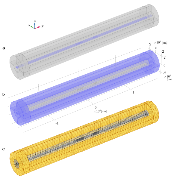
Figure 9: The COMSOL simulation geometry used for coupled modes consists of 30.5 $\mu$m long nanobeam (see Figs. 2 and 4a for beam design) with a 2.25 $\mu$m PML in the $x$ direction. The radial PML is 1.5 $\mu$m thick and is separated by a 1 $\mu$m buffer from the beam center. a Domain highlighted in blue indicates the embedded nanobeam with silicon material parameters. The surrounding domains (grey) use fictitious material parameters approximating a vacuum for inhomogeneous simulations, and use silicon material parameters for the homogeneous simulation. b Regions highlighted in blue show the PML domain, where we have cut out a quadrant of the radial PML to show the interior domains. c Domains highlighted in yellow show the radial PML regions, using a swept mesh with 5 layers. Remaining domains (grey) use a free tetrahedral mesh (see Table 1 for mesh parameters).

Appendix C COMSOL calculations and numerical Purcell factors

The power emission spectrum is obtained numerically by integrating the mechanical flux $\bm{I}$ over a small sphere around the point load. The mechanical flux is given by:

$$\bm{I}=-\bm{\sigma}\cdot\bm{v},$$ (34)

where $\bm{v}$ is the velocity vector. Power flow calculations in COMSOL were found to be sensitive to mesh geometry, with $P_{\rm inhomo}$ (nanobeam cavity) and $P_{0}$ (homogeneous bulk material) fluctuating dramatically with small changes in mesh parameters. However, $P_{\rm inhom}/P_{0}$ was found to be more convergent provided that the mesh geometry in the simulation of the beam be exactly identical to the simulation mesh of the homogeneous medium. This was achieved by using the same geometry and mesh points for both $P_{\rm inhom}$ and $P_{0}$ simulations, with the material parameters surrounding the beam (see Figure 9a) changed from silicon (homogeneous case) to a fictitious material with elasticity $(C_{11},C_{12},C_{44})=(0,0,0)$ GPa and a density of $0.001$ ${\rm kg}/{\rm m}^{3}$ in order to approximate a vacuum (inhomogeneous case). The fictitious material is necessary as meshes in the COMSOL solid mechanics solver must be assigned a material, and the chosen elasticity and density for the vacuum approximation suffice. In fact, we found that using any density less than $0.01$ ${\rm kg}/{\rm m}^{3}$ has negligible effect on the calculated $P_{\rm inhom}$ and the calculated eigenfrequencies of the QNMs (which agree with the in-vacuum simulations).

Max. element size	1000 [nm]
Min. element size	0.1 [nm]
Max. element growth rate	1.5
Curvature factor	0.6
Resolution of narrow regions	0.5
Max. point load element size	0.2 [nm]

Table 1: COMSOL simulation mesh parameters used.

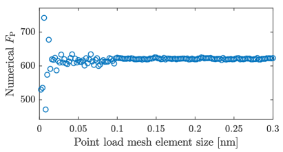
Figure 10: COMSOL simulations of the numerical Purcell factor (Eq. 27) of a mechanical mode at a single arbitrary frequency and dipole position for various maximum point load mesh element sizes.

Table 1 outlines the COMSOL mesh parameters used in our simulations, which were found to give consistent (and computationally feasible) solutions provided that an appropriate mesh element size is used for the point load. For absorbing boundary conditions, PMLs with polynomial coordinate stretching are used with the scaling factor and curvature parameter set to 1.

Figures 9b and  9c outline the PML simulation domains and their meshing type (see figure caption text). Figure 10 shows a parameter sweep of the maximum mesh element size assigned to the point load, where we can see convergence with small fluctuation for element sizes larger than 0.1 nm. For calculations in this work, a point load mesh element size of around 0.2 nm is used. Small shifts in this parameter (in the region of convergence) effectively minutely changes the simulation mesh, resulting in the fluctuations around the solution. In order to account for this, we take the average solution of simulations with slightly varied mesh sizes.

References

- Purcell et al. (1946) E. M. Purcell, H. C. Torrey, and R. V. Pound, “Resonance Absorption by Nuclear Magnetic Moments in a Solid,” Physical Review 69, 37–38 (1946).
- Kristensen et al. (2012) P. T. Kristensen, C. Van Vlack, and S. Hughes, “Generalized effective mode volume for leaky optical cavities,” Optics Letters 37, 1649–1651 (2012).
- Kristensen et al. (2020) Philip Trøst Kristensen, Kathrin Herrmann, Francesco Intravaia, Kurt Busch, and Kurt Busch, “Modeling electromagnetic resonators using quasinormal modes,” Advances in Optics and Photonics 12, 612–708 (2020).
- Kristensen and Hughes (2014) Philip Trøst Kristensen and Stephen Hughes, “Modes and Mode Volumes of Leaky Optical Cavities and Plasmonic Nanoresonators,” ACS Photonics 1, 2–10 (2014).
- Sauvan et al. (2013) C. Sauvan, J. P. Hugonin, I. S. Maksymov, and P. Lalanne, “Theory of the spontaneous optical emission of nanosize photonic and plasmon resonators,” Phys. Rev. Lett. 110, 237401 (2013).
- Ge et al. (2014) Rong Chun Ge, Philip Trøst Kristensen, Jeff F. Young, and Stephen Hughes, “Quasinormal mode approach to modelling light-emission and propagation in nanoplasmonics,” New Journal of Physics 16, 113048 (2014).
- KamandarDezfouli et al. (2017) Mohsen KamandarDezfouli, Reuven Gordon, and Stephen Hughes, “Modal theory of modified spontaneous emission of a quantum emitter in a hybrid plasmonic photonic-crystal cavity system,” Physical Review A 95, 013846 (2017).
- Franke et al. (2019) Sebastian Franke, Stephen Hughes, Mohsen Kamandar Dezfouli, Philip Trøst Kristensen, Kurt Busch, Andreas Knorr, and Marten Richter, “Quantization of Quasinormal Modes for Open Cavities and Plasmonic Cavity Quantum Electrodynamics,” Physical Review Letters 122, 213901 (2019).
- Franke et al. (2020) Sebastian Franke, Marten Richter, Juanjuan Ren, Andreas Knorr, and Stephen Hughes, “Quantized quasinormal-mode description of nonlinear cavity-qed effects from coupled resonators with a fano-like resonance,” Phys. Rev. Research 2, 033456 (2020).
- Bliokh and Nori (2019) Konstantin Y. Bliokh and Franco Nori, “Spin and orbital angular momenta of acoustic beams,” Phys. Rev. B 99, 174310 (2019).
- Eichenfield et al. (2009a) Matt Eichenfield, Ryan Camacho, Jasper Chan, Kerry J. Vahala, and Oskar Painter, “A picogram- and nanometre-scale photonic-crystal optomechanical cavity,” Nature 459, 550–555 (2009a).
- Aspelmeyer et al. (2014) Markus Aspelmeyer, Tobias J. Kippenberg, and Florian Marquardt, “Cavity optomechanics,” Reviews of Modern Physics 86, 1391–1452 (2014).
- Aspelmeyer et al. (2010) M. Aspelmeyer, S. Gröblacher, K. Hammerer, and N. Kiesel, “Quantum optomechanics—throwing a glance [Invited],” JOSA B 27, A189–A197 (2010).
- Kippenberg and Vahala (2007) T. J. Kippenberg and K. J. Vahala, “Cavity Opto-Mechanics,” Optics Express 15, 17172–17205 (2007).
- Favero and Karrai (2009) Ivan Favero and Khaled Karrai, “Optomechanics of deformable optical cavities,” Nature Photonics 3, 201–205 (2009).
- Verhagen et al. (2012) E. Verhagen, S. Deléglise, S. Weis, A. Schliesser, and T. J. Kippenberg, “Quantum-coherent coupling of a mechanical oscillator to an optical cavity mode,” Nature 482, 63–67 (2012).
- Weis et al. (2010) Stefan Weis, Rémi Rivière, Samuel Deléglise, Emanuel Gavartin, Olivier Arcizet, Albert Schliesser, and Tobias J. Kippenberg, “Optomechanically induced transparency,” Science 330, 1520–1523 (2010).
- Balram et al. (2016) Krishna C. Balram, Marcelo I. Davanço, Jin Dong Song, and Kartik Srinivasan, “Coherent coupling between radiofrequency, optical and acoustic waves in piezo-optomechanical circuits,” Nature Photonics 10, 346–352 (2016).
- Fiore et al. (2011) Victor Fiore, Yong Yang, Mark C. Kuzyk, Russell Barbour, Lin Tian, and Hailin Wang, “Storing Optical Information as a Mechanical Excitation in a Silica Optomechanical Resonator,” Physical Review Letters 107, 133601 (2011).
- Bagheri et al. (2011) Mahmood Bagheri, Menno Poot, Mo Li, Wolfram P. H. Pernice, and Hong X. Tang, “Dynamic manipulation of nanomechanical resonators in the high-amplitude regime and non-volatile mechanical memory operation,” Nature Nanotechnology 6, 726–732 (2011).
- Yu et al. (2016) Wenyan Yu, Wei C. Jiang, Qiang Lin, and Tao Lu, “Cavity optomechanical spring sensing of single molecules,” Nature Communications 7, 1–9 (2016).
- Liu et al. (2013) Fenfei Liu, Seyedhamidreza Alaie, Zayd C. Leseman, and Mani Hossein-Zadeh, “Sub-pg mass sensing and measurement with an optomechanical oscillator,” Optics Express 21, 19555–19567 (2013).
- Lau and Clerk (2020) Hoi-Kwan Lau and Aashish A. Clerk, “Ground-state cooling and high-fidelity quantum transduction via parametrically driven bad-cavity optomechanics,” Physical Review Letters 124 (2020), 10.1103/physrevlett.124.103602.
- Sankey et al. (2010) J. C. Sankey, C. Yang, B. M. Zwickl, A. M. Jayich, and J. G. E. Harris, “Strong and tunable nonlinear optomechanical coupling in a low-loss system,” Nature Physics 6, 707–712 (2010).
- Yablonovitch (1987) Eli Yablonovitch, “Inhibited Spontaneous Emission in Solid-State Physics and Electronics,” Physical Review Letters 58, 2059–2062 (1987).
- Krauss et al. (1996) Thomas F. Krauss, Richard M. De La Rue, and Stuart Brand, “Two-dimensional photonic-bandgap structures operating at near-infrared wavelengths,” Nature 383, 699–702 (1996).
- Kushwaha et al. (1993) M. S. Kushwaha, P. Halevi, L. Dobrzynski, and B. Djafari-Rouhani, “Acoustic band structure of periodic elastic composites,” Physical Review Letters 71, 2022–2025 (1993).
- Sigalas and Economou (1993) M. Sigalas and E. N. Economou, “Band structure of elastic waves in two dimensional systems,” Solid State Communications 86, 141–143 (1993).
- Maldovan (2013) Martin Maldovan, “Sound and heat revolutions in phononics,” Nature 503, 209–217 (2013).
- Laude (2016) V. Laude, “Phoxonic crystals for harnessing the interaction of light and sound,” in 2016 International Conference on Optical MEMS and Nanophotonics (OMN) (2016) pp. 1–2.
- Rolland et al. (2012) Q. Rolland, M. Oudich, S. El-Jallal, S. Dupont, Y. Pennec, J. Gazalet, J. C. Kastelik, G. Lévêque, and B. Djafari-Rouhani, “Acousto-optic couplings in two-dimensional phoxonic crystal cavities,” Applied Physics Letters 101, 061109 (2012).
- El Hassouani et al. (2010) Y. El Hassouani, C. Li, Y. Pennec, E. H. El Boudouti, H. Larabi, A. Akjouj, O. Bou Matar, V. Laude, N. Papanikolaou, A. Martinez, and B. Djafari Rouhani, “Dual phononic and photonic band gaps in a periodic array of pillars deposited on a thin plate,” Physical Review B 82, 155405 (2010).
- Djafari-Rouhani et al. (2016) Bahram Djafari-Rouhani, Said El-Jallal, and Yan Pennec, “Phoxonic crystals and cavity optomechanics,” Comptes Rendus Physique Phononic crystals / Cristaux phononiques, 17, 555–564 (2016).
- Kipfstuhl et al. (2014) Laura Kipfstuhl, Felix Guldner, Janine Riedrich-Möller, and Christoph Becher, “Modeling of optomechanical coupling in a phoxonic crystal cavity in diamond,” Optics Express 22, 12410–12423 (2014).
- Eichenfield et al. (2009b) Matt Eichenfield, Jasper Chan, Amir H. Safavi-Naeini, Kerry J. Vahala, and Oskar Painter, “Modeling dispersive coupling and losses of localized optical and mechanical modes in optomechanical crystals,” Optics Express 17, 20078–20098 (2009b).
- Chan et al. (2012) Jasper Chan, Amir H. Safavi-Naeini, Jeff T. Hill, Seán Meenehan, and Oskar Painter, “Optimized optomechanical crystal cavity with acoustic radiation shield,” Applied Physics Letters 101, 081115 (2012).
- Kalaee et al. (2016) M. Kalaee, T. K. Paraïso, H. Pfeifer, and O. Painter, “Design of a quasi-2d photonic crystal optomechanical cavity with tunable, large x-coupling,” Optics Express 24, 21308–21328 (2016).
- Pitanti et al. (2015) Alessandro Pitanti, Johannes M. Fink, Amir H. Safavi-Naeini, Jeff T. Hill, Chan U. Lei, Alessandro Tredicucci, and Oskar Painter, “Strong opto-electro-mechanical coupling in a silicon photonic crystal cavity,” Optics Express 23, 3196–3208 (2015).
- Krause et al. (2012) Alexander G. Krause, Martin Winger, Tim D. Blasius, Qiang Lin, and Oskar Painter, “A high-resolution microchip optomechanical accelerometer,” Nature Photonics 6, 768–772 (2012).
- Winger et al. (2011) M. Winger, T. D. Blasius, T. P. Mayer Alegre, A. H. Safavi-Naeini, S. Meenehan, J. Cohen, S. Stobbe, and O. Painter, “A chip-scale integrated cavity-electro-optomechanics platform,” Optics Express 19, 24905–24921 (2011).
- Johansson et al. (2014) J. R. Johansson, G. Johansson, and Franco Nori, “Optomechanical-like coupling between superconducting resonators,” Physical Review A 90, 053833 (2014).
- Schmidt et al. (2018) Mikołaj K. Schmidt, L.G. Helt, Christopher G. Poulton, and M.J. Steel, “Elastic Purcell Effect,” Physical Review Letters 121, 064301 (2018).
- Landi et al. (2018) Maryam Landi, Jiajun Zhao, Wayne E. Prather, Ying Wu, and Likun Zhang, “Acoustic Purcell Effect for Enhanced Emission,” Physical Review Letters 120, 114301 (2018).
- Lasson et al. (2015) Jakob Rosenkrantz de Lasson, Philip Trøst Kristensen, Jesper Mørk, and Niels Gregersen, “Semianalytical quasi-normal mode theory for the local density of states in coupled photonic crystal cavity–waveguide structures,” Optics Letters 40, 5790–5793 (2015).
- Lalanne et al. (2018) Philippe Lalanne, Wei Yan, Kevin Vynck, Christophe Sauvan, and Jean-Paul Hugonin, “Light Interaction with Photonic and Plasmonic Resonances,” Laser & Photonics Reviews 12, 1700113 (2018).
- Pinard et al. (1999) M. Pinard, Y. Hadjar, and A. Heidmann, “Effective mass in quantum effects of radiation pressure,” European Physical Journal D 7, 107–116 (1999).
- Gillespie and Raab (1995) A. Gillespie and F. Raab, “Thermally excited vibrations of the mirrors of laser interferometer gravitational-wave detectors,” Physical Review D 52, 577–585 (1995).
- Li et al. (2015) Yongzhuo Li, Kaiyu Cui, Xue Feng, Yidong Huang, Zhilei Huang, Fang Liu, and Wei Zhang, “Optomechanical crystal nanobeam cavity with high optomechanical coupling rate,” Journal of Optics 17, 045001 (2015).
- Zheng et al. (2012) Jiangjun Zheng, Xiankai Sun, Ying Li, Menno Poot, Ali Dadgar, Norman Nan Shi, Wolfram H. P. Pernice, Hong X. Tang, and Chee Wei Wong, “Femtogram dispersive L3-nanobeam optomechanical cavities: design and experimental comparison,” Optics Express 20, 26486–26498 (2012).
- Yao et al. (2010) P. Yao, V. S. C. Manga Rao, and S. Hughes, “On-chip single photon sources using planar photonic crystals and single quantum dots,” Laser & Photonics Reviews 4, 499–516 (2010).
- Limonov et al. (2017) Mikhail F. Limonov, Mikhail V. Rybin, Alexander N. Poddubny, and Yuri S. Kivshar, “Fano resonances in photonics,” Nature Photonics 11, 543–554 (2017).
- Khanikaev et al. (2013) Alexander B. Khanikaev, Chihhui Wu, and Gennady Shvets, “Fano-resonant metamaterials and their applications,” Nanophotonics 2, 247–264 (2013).
- Luk’yanchuk et al. (2010) Boris Luk’yanchuk, Nikolay I. Zheludev, Stefan A. Maier, Naomi J. Halas, Peter Nordlander, Harald Giessen, and Chong Tow Chong, “The Fano resonance in plasmonic nanostructures and metamaterials,” Nature Materials 9, 707–715 (2010).
- Qu and Agarwal (2013) Kenan Qu and G. S. Agarwal, “Fano resonances and their control in optomechanics,” Physical Review A 87, 063813 (2013).
- Abbas et al. (2019) Muqaddar Abbas, Rahmat Ullah, You-Lin Chuang, and Ziauddin, “Investigation of Fano resonances in the optomechanical cavity via a magnetic field,” Journal of Modern Optics 66, 176–182 (2019).
- Heuck et al. (2013) Mikkel Heuck, Philip Trøst Kristensen, Yuriy Elesin, and Jesper Mørk, “Improved switching using fano resonances in photonic crystal structures,” Optics Letters 38, 2466 (2013).
- Luk’yanchuk et al. (2013) B. S. Luk’yanchuk, A. E. Miroshnichenko, and Yu S. Kivshar, “Fano resonances and topological optics: an interplay of far- and near-field interference phenomena,” Journal of Optics 15, 073001 (2013).
- Chen et al. (2015) Huajin Chen, Shiyang Liu, Jian Zi, and Zhifang Lin, “Fano Resonance-Induced Negative Optical Scattering Force on Plasmonic Nanoparticles,” ACS Nano 9, 1926–1935 (2015).
- Stassi et al. (2017) Stefano Stassi, Alessandro Chiadò, Giuseppe Calafiore, Gianluca Palmara, Stefano Cabrini, and Carlo Ricciardi, “Experimental evidence of Fano resonances in nanomechanical resonators,” Scientific Reports 7, 1065 (2017).
- Lin et al. (2010) Qiang Lin, Jessie Rosenberg, Darrick Chang, Ryan Camacho, Matt Eichenfield, Kerry J. Vahala, and Oskar Painter, “Coherent mixing of mechanical excitations in nano-optomechanical structures,” Nature Photonics 4, 236–242 (2010).
- Barth et al. (2010) Michael Barth, Stefan Schietinger, Sabine Fischer, Jan Becker, Mils Nüsse, Thomas Aichele, Bernd Löchel, Carsten Sönnichsen, and Oliver Benson, “Nanoassembled plasmonic-photonic hybrid cavity for tailored light-matter coupling,” Nano Letters 10, 891–895 (2010).
- Doeleman et al. (2016) Hugo M. Doeleman, Ewold Verhagen, and A. Femius Koenderink, “Antenna–cavity hybrids: Matching polar opposites for purcell enhancements at any linewidth,” ACS Photonics 3, 1943–1951 (2016).
- Slaughter (2002) William S. Slaughter, The Linearized Theory of Elasticity (Birkhäuser Boston, 2002).
- Snieder (2002) Roel Snieder, “Chapter 1.7.1 - General Theory of Elastic Wave Scattering,” in Scattering, edited by Roy Pike and Pierre Sabatier (Academic Press, London, 2002) pp. 528–542.
- Lee et al. (1999) K. M. Lee, P. T. Leung, and K. M. Pang, “Dyadic formulation of morphology-dependent resonances. I. Completeness relation,” JOSA B 16, 1409–1417 (1999).
- Kristensen et al. (2015) Philip Trøst Kristensen, Rong-Chun Ge, and Stephen Hughes, “Normalization of quasinormal modes in leaky optical cavities and plasmonic resonators,” Physical Review A 92, 053810 (2015).
- Muljarov et al. (2010) E. A. Muljarov, W. Langbein, and R. Zimmermann, “Brillouin-wigner perturbation theory in open electromagnetic systems,” EPL (Europhysics Letters) 92, 50010 (2010).
- Bai et al. (2013) Q. Bai, M. Perrin, C. Sauvan, J.-P. Hugonin, and P. Lalanne, “Efficient and intuitive method for the analysis of light scattering by a resonant nanostructure,” Optics Express 21, 27371–27382 (2013).
- Zschiedrich et al. (2018) Lin Zschiedrich, Felix Binkowski, Niko Nikolay, Oliver Benson, Günter Kewes, and Sven Burger, “Riesz-projection-based theory of light-matter interaction in dispersive nanoresonators,” Phys. Rev. A 98, 043806 (2018).
- Lai et al. (1990) H. M. Lai, P. T. Leung, K. Young, P. W. Barber, and S. C. Hill, “Time-independent perturbation for leaking electromagnetic modes in open systems with application to resonances in microdroplets,” Physical Review A 41, 5187–5198 (1990).
- Novotny and Hecht (2006) Lukas Novotny and Bert Hecht, Principles of Nano-Optics (Cambridge University Press, 2006).