Big-bang nucleosynthesis with sub-GeV massive decaying particles

Abstract

We consider the effects of the injections of energetic photon and electron (or positron) on the big-bang nucleosynthesis. We study the photodissociation of light elements in the early Universe paying particular attention to the case that the injection energy is sub-GeV and derive upper bounds on the primordial abundances of the massive decaying particle as a function of its lifetime. We also discuss a solution of the ⁷Li problem in this framework.

KEK-Cosmo-254, KEK-TH-2214

1 Introduction

Big-bang nucleosynthesis (BBN) provides a powerful probe of the thermal history of the Universe. In the standard BBN (SBBN) scenario, the light elements (i.e., D, ³He, ⁴He, and so on) are synthesized at the cosmic time of $t\gtrsim 1\ {\rm sec}$ (corresponding to the cosmic temperature of $T\lesssim 1\ {\rm MeV}$) at which the typical energy of the background photon becomes much lower than the binding energies of nuclei. Because the predictions of the SBBN are more or less in good agreements with the observations of the primordial abundances of light elements [1], beyond-the-standard-model (BSM) physics which alters the thermal history after $\sim 1\ {\rm sec}$ may be constrained or excluded in order not to spoil the success of the SBBN.

One important class of BSM models affecting the light element abundances is that with long-lived particles. In many BSM models, there shows up a long-lived particle whose lifetime is longer than $\sim 1\ {\rm sec}$. If such a long-lived particle is somehow produced in the early Universe, and also if it decays into standard-model particles, its late-time decay causes hadronic and electromagnetic showers after the BBN epoch. Energetic particles in the showers dissociate light elements, resulting in the change of their abundances. The effects of radiative decay of long-lived particles on the light element abundances have been intensively studied in Refs. [2, 3, 4, 5, 6, 7, 8, 9, 10, 11, 12, 13, 14, 15] and references therein (see also Refs. [16, 17, 18, 10, 11, 12, 13, 14, 15] for hadronic decays). Many of previous studies paid particular attention to the case where the mass of the long-lived particle is around or above the electroweak scale, which is motivated by the relation between the BSM physics and the electroweak scale. In particular, in the thermal relic dark matter scenario, the pair annihilation cross section of the dark matter particle is about $1\ \rm{\rm pb}$, corresponding to the cross section obtained by the exchange of particle with mass around the electroweak scale (assuming that the coupling constant is sizable). It motivates us to consider BSM models for dark matter whose typical mass scale is around the electroweak scale.

Recently, however, models with sub-GeV dark matter have been attracting much attention [19, 20, 21, 22, 23]. In such models, the masses of particles other than the dark matter particle are also often sub-GeV. Importantly, in certain models [24], some of the particles in the model become long-lived and may have lifetime longer than $\sim 1\ {\rm sec}$. If so, such long-lived particles may affect the light element abundances. Effects of sub-GeV long-lived particles on the BBN significantly differs from those of heavier ones.

• If the mass of the long-lived particle is around the electroweak scale (or higher), significant amount of hadrons are expected to be produced by the decay, causing hadronic shower in the thermal plasma in the early Universe [16, 17, 18, 10, 11, 12, 13, 14, 15]. Then, the hadrodissociation process often gives stringent constraints on the model [15] (even though electromagnetic shower also occurs). For the case of sub-GeV long-lived particle, on the contrary, productions of hadrons at the time of the decay are kinematically suppressed (or forbidden). In such a case, effects of photodissociation processes of light elements become more important.

• With the injection of energetic photons (or electrons and positrons) into thermal plasma, electromagnetic showers are induced. The photon spectrum in the showers is (approximately) determined by the total amount of energy injection if the energy of primary photons is large enough [4, 5]. If the energy of the primary photon is sub-GeV, on the contrary, such a universal behavior of the spectrum is lost and the shape of the spectrum becomes sensitive to the energy of the injected photons [25, 26, 27] (See also [28]). Thus, for the study of the BBN constraints on the sub-GeV long-lived particles, a careful calculation of the photon spectrum in the electromagnetic shower is needed.

Thus, a detailed study about the effects of sub-GeV long-lived particles on the BBN predictions should be necessary.

Motivated by these observations, we study the light element abundances in models with sub-GeV long-lived particles. We concentrate on the case where the unstable particle decays into photon or electron and positron, assuming that the decay processes into other particles (in particular, hadrons) are kinematically suppressed or forbidden.

The organization of this paper is as follows. In Section 2, we summarize the observational abundances of light elements. In Section 3, we discuss our treatment of the electromagnetic shower induced by the injection of the electromagnetic particles into the thermal bath in the early Universe. In Section 4, we discuss the entropy production which also plays important role in constraining the long-lived particles. The constraints on the primordial abundance of long-lived particles are given in Section 5. A possibility to solve the ⁷Li problem using long-lived particles are discussed in Section 6. Section 7 is devoted to conclusions and discussion.

In this paper, we adopt natural units, $c=\hbar=1$, and $n_{i}$ indicates the number density of species “i.” In addition, yield variable is defined as

$$Y_{i}\equiv\frac{n_{i}}{s},$$ (1.1)

with $s$ being the entropy density.

2 Observational Abundances of Light Elements

In this section we summarize observational constraints on the primordial abundances of light elements (D, ³He, ⁴He and ⁷Li). The errors are written at 68$\%$ C.L. unless otherwise noted. The subscript $p$ denotes the primordial value.

• D
  The deuterium abundance has been precisely measured by observing absorption of QSO lights due to damped Lyman-$\alpha$ systems. We adopt

  $$(\text{D}/\text{H})_{p}=(2.545\pm 0.025)\times 10^{-5},$$ (2.1)

  from measurements of 13 damped Lyman-$\alpha$ systems [31]. This abundance is consistent with another recent value $(\text{D}/\text{D})_{p}=(2.527\pm 0.030)\times 10^{-5}$ reported by Cooke et al. [32].

• ³He
  We adopt the observed ³He/D as an upper bound on the primordial value [33]. From ³He and D abundances observed in protosolar clouds [34], we adopt

  $$({\rm{}^{3}He}/{\rm D})_{p}<0.83+0.27.$$ (2.2)

• ⁴He
  The primordial abundance of ⁴He is determined by measurement of recombination lines from extra-galactic HII regions. Izotov et al. [35] obtained $Y_{p}=0.2551\pm 0.0022$ from the observation of 45 extragalactic HII regions. Aver, Olive and Skillman [36] reanalyzed the data of Ref. [35] and obtained $Y_{p}=0.2449\pm 0.0040$ which is inconsistent with the value given in [35]. More recently Fernández et al. [37] reported $Y_{p}=0.245\pm 0.007$ using 27 HII regions selected SDSS. Valerdi et al. [38] obtained $Y_{p}=0.2451\pm 0.0026$ from the observation of the HII region in NGC 246. These recent measurements are in good agreement with result of [36]. Therefore, in this paper we adopt the value obtained by Aver, Olive and Skillman [36],

  $$Y_{p}=0.2449\pm 0.0040.$$ (2.3)

• ⁷Li
  Observations of ⁷Li abundances in atmospheres of metal-poor halo stars show an almost constant value called ”Spite plateau” which has been considered as primordial. Bonifacio et al [39] reported the ⁷Li abundance as

  $${\rm Log}_{10}\left({{}^{7}{\rm Li}}/{\rm H}\right)_{p}=-9.900\pm 0.090.$$ (2.4)

  However, the above abundance is about three times smaller than that predicted in the standard BBN. This discrepancy between the BBN prediction and observation is called “⁷Li problem.” However, recent observations of extremely metal-poor stars show abundance much smaller than the Spite plateau value [40]. If we take such recent observations seriously, some unknown physical processes should change the ⁷Li abundances during or after the BBN. Thus, it may be still premature to regard the abundance given in Eq. (2.4) as a primordial abundance of ⁷Li. In the following, we will derive upper bounds on the primordial abundance of the unstable particle $X$. In such an analysis, we try to be conservative so that we do not use ⁷Li abundances for the study of the bound. In addition, we will also discuss the implication of the long-lived particle on the ⁷Li problem. We will show that MeV decaying particles may give a solution to the ⁷Li problem if the plateau abundance (2.4) is primordial [39] (and lower abundances in extremely metal-poor stars is realized by another process, e.g. [41]).

Here we also mention other observational constraints used in the present paper. The baryon to photon ratio is taken to be

$$\eta=(6.13\pm 0.04)\times 10^{-10},$$ (2.5)

which is based on the density parameter for baryon $\Omega_{\rm B}h^{2}=0.02237^{+0.00015}_{-0.00015}$ (68$\%$ C.L.) for the TT,TE,EE+lowE+lensing analysis by the Planck collaboration, where $h$ is the Hubble constant in units of $100\ {\rm km/sec/Mpc}$ [29].

The Planck collaboration also reported constraints on the effective number of neutrino species. We adopt the following value in the same case as that of $\eta$ by the TT,TE,EE+lowE (+lensing) analysis,

$$N_{\nu}^{\rm eff}=2.92^{+0.36}_{-0.37},$$ (2.6)

at 95$\%$ C.L.  [29]. That means $N_{\nu}^{\rm eff}$ can ranges 2.55 – 3.28 at 95$\%$ C.L. where the lower limit $N_{\nu}^{\rm eff}>N_{\nu,{\rm low}}^{\rm eff}=2.55$ is important to constrain late-time injections of electromagnetic energy produced by massive particles decaying at $T\ll 1$ MeV [30].

3 Electromagnetic Shower

In this section, we discuss how we treat the electromagnetic shower induced by the decaying particle (which we call $X$). We follow the procedure explained in Refs. [3, 4].

For the cosmic temperature of our interest, relevant scattering processes induced by energetic photons are as follows.

• Double photon pair creation: $\gamma+\gamma_{\rm BG}\rightarrow e^{+}+e^{-}$.

• Photon photon scattering: $\gamma+\gamma_{\rm BG}\rightarrow\gamma+\gamma$.

• Pair creation in nuclei: $\gamma+N_{\rm BG}\rightarrow\gamma+e^{+}+e^{-}$.

• Compton Scattering: $\gamma+e^{-}_{\rm BG}\rightarrow\gamma+e^{-}$.

In addition, energetic electron (as well as positron) loses its energy via

• Inverse Compton scattering: $e^{\pm}+\gamma_{\rm BG}\rightarrow e^{\pm}+\gamma$.

Here, the subscript “BG” is for particles in the background and $N_{\rm BG}$ denotes the background nuclei.

We concentrate on the case where the scattering rates of photons and electrons are larger than the expansion rate of the Universe. Then, neglecting the effects of the cosmic expansion, the Boltzmann equations for the distribution function of photons (denoted as $f_{\gamma}$) and that of electrons plus positrons (denoted as $f_{e}$) are denoted as

$$\frac{\partial f_{\gamma}(E_{\gamma})}{\partial t}= \left[\frac{\partial f_{\gamma}(E_{\gamma})}{\partial t}\right]_{\rm DP}+\left[\frac{\partial f_{\gamma}(E_{\gamma})}{\partial t}\right]_{\rm PP}+\left[\frac{\partial f_{\gamma}(E_{\gamma})}{\partial t}\right]_{\rm PC}+\left[\frac{\partial f_{\gamma}(E_{\gamma})}{\partial t}\right]_{\rm CS}+\left[\frac{\partial f_{\gamma}(E_{\gamma})}{\partial t}\right]_{\rm IC}$$

$$+\left[\frac{\partial f_{\gamma}(E_{\gamma})}{\partial t}\right]_{\rm DE},$$ (3.1)

$$\frac{\partial f_{e}(E_{e})}{\partial t}= \left[\frac{\partial f_{e}(E_{e})}{\partial t}\right]_{\rm DP}+\left[\frac{\partial f_{e}(E_{e})}{\partial t}\right]_{\rm PC}+\left[\frac{\partial f_{e}(E_{e})}{\partial t}\right]_{\rm CS}+\left[\frac{\partial f_{e}(E_{e})}{\partial t}\right]_{\rm IC}+\left[\frac{\partial f_{e}(E_{e})}{\partial t}\right]_{\rm DE},$$ (3.2)

where terms with the index DP (PP, PC, CS, IC, and DE) represents the contribution from the double photon pair creation process (photon-photon scattering, pair creation in nuclei, Compton scattering, Inverse Compton scattering, and decay of the exotic particle). Explicit forms of individual terms are given in Ref. [4].

Hereafter, for simplicity, we concentrate on the case that the energy of the particles produced by the decay is monochromatic (and is denoted as $\epsilon_{0}$) except for the final-state radiation (FSR). Then, the decay terms take a simple form:

• For the case of monochromatic photon injection from the decay, the decay terms are given by

  $$\left[\frac{\partial f_{\gamma}(E_{\gamma})}{\partial t}\right]_{\rm DE}=\, \xi_{\gamma}\frac{n_{X}}{\tau_{X}}\delta(E_{\gamma}-\epsilon_{0}),$$ (3.3)

  $$\left[\frac{\partial f_{e}(E_{e})}{\partial t}\right]_{\rm DE}=\, 0,$$ (3.4)

  where $n_{X}$ is the number density of $X$, $\tau_{X}$ is the lifetime of $X$, and $\xi_{\gamma}$ is the number of photon emitted by the decay of one $X$ particle.

• For the case where $X$ decays primarily into monochromatic electron and positron, energetic photons are also produced via FSR, as discussed in Ref. [27] (see also Appendix B for a generic case). Taking into account the effect of FSR, the decay terms are given by

  $$\left[\frac{\partial f_{\gamma}(E_{\gamma})}{\partial t}\right]_{\rm DE}=\, \xi_{e}\frac{n_{X}}{\tau_{X}\epsilon_{0}}\frac{\alpha}{2\pi}\frac{1+(1-x)^{2}}{x}\ln\left[\frac{4\epsilon_{0}^{2}(1-x)}{m_{e}^{2}}\right]\theta\left(1-\frac{m_{e}^{2}}{4\epsilon_{0}^{2}}-x\right),$$ (3.5)

  $$\left[\frac{\partial f_{e}(E_{e})}{\partial t}\right]_{\rm DE}=\, \xi_{e}\frac{n_{X}}{\tau_{X}}\delta(E_{e}-\epsilon_{0}),$$ (3.6)

  where $\alpha$ is the fine structure constant, and $x\equiv E_{\gamma}/\epsilon_{0}$. In addition, $\xi_{e}$ is the number of electrons and positrons produced by the decay of $X$. (If $X$ decays into a $e^{+}e^{-}$ pair, for example, $\xi_{e}=2$.)

We numerically solve Eqs. (3.1) and (3.2) to obtain the distribution functions of photons and electrons. Because the time scale of the shower evolution is much shorter than the time scale of the cosmic expansion, we solve the Boltzmann equations taking $\dot{f}_{\gamma}(E_{\gamma})=\dot{f}_{e}(E_{e})=0$ (with the “dot” indicating the derivative with respect to time) for each $t$, approximating $\dot{n}_{X}=0$.

In Figs. 2, 2, and 3, we show the photon spectrum induced by the injections of monochromatic photons and electrons, taking $E_{\rm in}=10\ {\rm MeV}$, $100\ {\rm MeV}$, and $1\ {\rm GeV}$, respectively. The singular peaks at $E_{\gamma}=\epsilon_{0}$ are due to the monochromatic injection of the photons.

We can see that, for the case of the electron injection, the FSR photons significantly affect the photon spectrum in particular when the cosmic temperature becomes low. This is because, when $X$ primarily decays into a $e^{+}e^{-}$ pair, the electromagnetic shower is initiated by the FSR photons as well as Inverse Compton scattering process $e^{\pm}+\gamma_{\rm BG}\rightarrow e^{\pm}\gamma$. When the electron becomes non-relativistic in the center-of-mass frame, the energy transfer of the final-state photon in the Inverse Compton process becomes typically $\sim T$. Because we are interested in the photons spectrum for $E_{\gamma}\gtrsim O(1)\ {\rm MeV}$ for the study of the photodissociation processes, the Inverse Compton process becomes unimportant in such a case. The FSR photons are, on the contrary, more energetic and can affect the photon spectrum relevant for the photodissociation. The FSR photons carry away only a fraction of the energy (i.e., the mass of $X$). Thus, the photon spectrum mainly initiated by the FSR photons is suppressed compared to the case of the energetic photon injection. This has significant implication for the BBN constraints on unstable particles as we will discuss below.

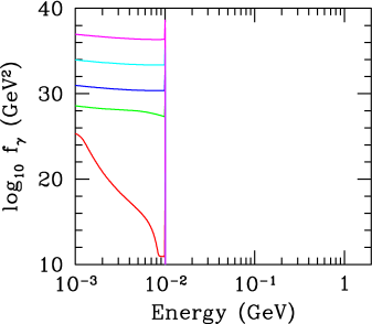
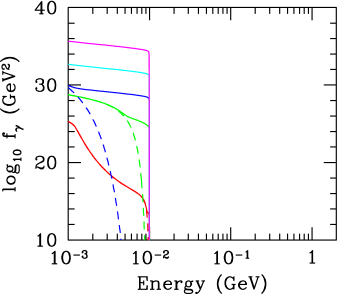
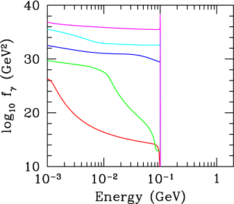
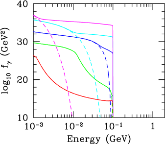
Figure 1: Photon spectrum induced by monochromatic photon (left) and electron (right) injection, taking $\epsilon_{0}=10\ {\rm MeV}$. The cosmic temperature is $10^{-5}$, $10^{-6}$, $10^{-7}$, $10^{-8}$, and $10^{-9}\ {\rm GeV}$, from below. Here, we take $n_{X}=1\ {\rm GeV}^{3}$. For the case of the monochromatic electron injection, the solid lines show the spectrum with the effect of FSR, while the dashed lines show the spectrum with neglecting the effect of FSR (taking $[\dot{f}_{\gamma}]_{\rm DE}=0$, instead of Eq. (3.5)).

Figure 2: Same as Fig. 2, except for $E_{\rm in}=100\ {\rm MeV}$.

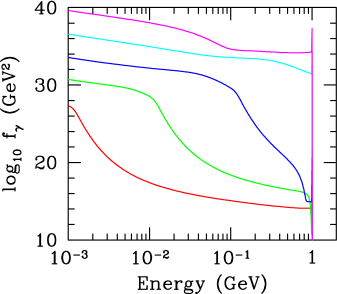
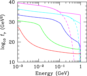
Figure 3: Same as Fig. 2, except for $E_{\rm in}=1\ {\rm GeV}$.

For the case of the injection of monochromatic electron, we observe deviation of our photon spectrum from those of [27]; for some choice of parameters, our photon spectrum is smaller by a factor of $\sim 2$. We expect that the deviation originates from the difference of the treatment of the effect of Compton scattering at small $y_{e}\equiv E_{e}T/m_{e}^{2}$. The energy-loss rate of the electron in thermal bath is given by [42]

$$\dot{E}_{e}=-\frac{4}{3}\sigma_{\rm T}\gamma_{e}^{2}\left[1-\frac{63}{10}\frac{\gamma_{e}\langle\epsilon_{\gamma}^{2}\rangle}{m_{e}\langle\epsilon_{\gamma}\rangle}+\cdots\right]\rho_{\gamma},$$ (3.7)

where $\langle\epsilon_{\gamma}\rangle$ and $\langle\epsilon_{\gamma}^{2}\rangle$ are the mean energy and mean energy squared of the background photons, respectively, $\sigma_{\rm T}\equiv(8\pi/3)\alpha^{2}/m_{e}^{2}$, and $\gamma_{e}\equiv E_{e}/m_{e}$. In Ref. [27] the second and higher order terms in the square bracket are neglected for $y_{e}<0.05$. However, numerically, the second term in the square bracket is $\sim-24y_{e}$, and is sizable when $y_{e}\sim O(10^{-2})$. With neglecting higher order terms in $y_{e}$, the energy loss rate of the electron is overestimated, which may affect the photon spectrum induced by the decay of $X$.

Once the photon spectrum is obtained, the effects of the photodissociation processes can be included into the Boltzmann equations governing the evolution of light elements. The effects of the photodissociation are taken into account by adding the following terms into the scattering terms in the Boltzmann equations:

$$\left[\frac{dn_{A_{i}}}{dt}\right]_{\rm photodiss}\equiv-n_{A_{i}}\sum_{j}\Gamma_{A_{i}\rightarrow A_{j}}^{\rm(photodiss)}+\sum_{j}n_{A_{j}}\Gamma_{A_{j}\rightarrow A_{i}}^{\rm(photodiss)},$$ (3.8)

where $n_{A_{i}}$ is the number density of the nuclear species $A_{i}$, and

$$\Gamma_{A_{j}\rightarrow A_{i}}^{\rm(photodiss)}\equiv\int dE_{\gamma}\sigma_{A_{i}\rightarrow A_{j}}(E_{\gamma})f_{\gamma}(E_{\gamma}),$$ (3.9)

with $\sigma_{A_{i}\rightarrow A_{j}}$ being the cross section for the process $\gamma+A_{i}\rightarrow A_{j}+\cdots$. The photodissociation processes included in our analysis are summarized in Table 1. In our code, the dissociation processes of ⁶Li, ⁷Li, and ⁷Be are included. Because the abundances of these elements are much smaller than those of lighter ones, they do not affect the discussion in Section 5 to derive the upper bounds on the primordial abundance of $X$. In discussing the implication to the ⁷Li problem in Section 6, on the other hand, these processes (in particular, the dissociation of ⁷Be) play an important role.

Reaction	Error	Reference
$\gamma+{\rm D}\rightarrow n+p$	6 %	[43]
$\gamma+{\rm T}\rightarrow n+{\rm D}$	14%	[44, 45]
$\gamma+{\rm T}\rightarrow p+n+n$	7%	[45]
$\gamma+{\rm{}^{3}He}\rightarrow p+{\rm D}$	10%	[46]
$\gamma+{\rm{}^{3}He}\rightarrow p+p+n$	15%	[46]
$\gamma+{\rm{}^{4}He}\rightarrow p+{\rm T}$	4%	[47]
$\gamma+{\rm{}^{4}He}\rightarrow n+{{}^{3}{\rm He}}$	5%	[48, 49]
$\gamma+{\rm{}^{4}He}\rightarrow p+n+{\rm D}$	14%	[47]
$\gamma+{\rm{}^{6}Li}\rightarrow{\rm anything}$	4%	[50]
$\gamma+{\rm{}^{7}Li}\rightarrow n+{{}^{6}{\rm Li}}$	4%	[51]
$\gamma+{\rm{}^{7}Li}\rightarrow{\rm anything}$	9%	[52]
$\gamma+{\rm{}^{7}Be}\rightarrow{{}^{3}{\rm He}}+{{}^{4}{\rm He}}$	9%	[53]
$\gamma+{\rm{}^{7}Be}\rightarrow p+{{}^{6}{\rm Li}}$	4%	[9]
$\gamma+{\rm{}^{7}Be}\rightarrow p+p+n+{{}^{4}{\rm He}}$	9%	[9]

Table 1: Photodissociation processes included in our analysis. The errors of each cross sections adopted in our Monte Carlo analysis are also shown.

4 Late-time entropy production due to the decay of $X$

In this section, we discuss the so-called “dilution factor” of the relic particle by the late-time entropy production due to massive particles decaying into 100 $\%$ of electromagnetic energy, e.g., photons or electrons without producing neutrinos. In this case, we can approximately express the dilution factor to be

$$\Delta_{\rm dilution} = 1+\frac{\Delta s}{s}=\left(\frac{T_{\gamma a}}{T_{\gamma b}}\right)^{3}=\left(1+\frac{\Delta\rho_{\gamma}}{\rho_{\gamma}}\right)^{3/4},$$

where $T_{\gamma a}$ and $T_{\gamma b}$ mean approximately the photon temperature just after and just before the entropy production, respectively. Here we assume that electromagnetic particles are immediately thermalized, which is approximately validated well before the recombination epoch. In this expression, $\Delta s$ is the increase of the entropy density $s$ due to the decaying massive particles. Then the baryon to photon ratio is diluted after the entropy production to be

$$\eta(T_{\gamma a})=\frac{\eta(T_{\gamma b})}{\Delta_{\rm dilution}},$$ (4.1)

where $\eta(T_{\gamma a})$ could be observed by cosmic microwave background (CMB) experiments such as Planck (See Eq. (2.5)). Actually we set an initial value of $\eta$ to be $\eta(T_{\gamma b})$ well in advance before the entropy production, e.g., at $T\gg 10$ MeV with simultaneously fitting $\eta(T_{\gamma a})$ to be the required value in Eq. (2.5). In Appendix A, we show an analytical calculation of $\Delta_{\rm dilution}$ in a general setup in the parameter spaces. The analytical formula are consistent with actual computations of $\Delta_{\rm dilution}$ within a few percent accuracy in the parameter space where we are considering in the current study, e.g., for $\Delta_{\rm dilution}\lesssim{\cal O}(10)$.

After $T\ll 1$ MeV, if the copious entropy is produced by injection of electromagnetic energy due to decaying massive particles, the cosmic neutrinos cannot be thermalized.

Due to such a sizable dilution factor for $t\gg 1$ sec, the effective number of neutrino species is also modified to be $3.046\to 3.046-|\Delta N_{\nu}|$, which is constrained by the CMB observations (2.6) as

$$3.046-|\Delta N_{\nu}|=3.046\Delta_{\rm dilution}^{-4/3}>N_{\nu,{\rm low}}^{\rm eff},$$ (4.2)

where $N_{\nu,{\rm low}}^{\rm eff}=2.55$ at 95 $\%$ C.L. as is shown in (2.6). Thus, we obtain an upper bound on the modification of $N_{\nu}^{\rm eff}$,

$$|\Delta N_{\nu}|<3.046-N_{\nu,{\rm low}}^{\rm eff}\simeq 0.50,$$ (4.3)

which leads to an upper bound on the dilution factor

$$\Delta_{\rm dilution}<\left(\frac{3.046}{N_{\nu,{\rm low}}^{\rm eff}}\right)^{3/4}\simeq 1.14,$$ (4.4)

at 95 $\%$ C.L. By using the constraint on $\Delta N_{\nu}$ shown in (4.3), we can constrain parameters of the lifetime and the abundance of the decaying massive particles.

5 Results

Now we show BBN constraints on the injections of sub-GeV photons and electrons. In order to calculate abundances of light elements with their theoretical errors, we execute the Monte Carlo estimation by including errors in $\eta$, lifetime of neutron, and reaction rates in both the standard processes in SBBN and the non-standard photodissociation processes.

5.1 Injections of a high-energy line photon

First, let us consider the case of sub-GeV line photon. In Fig. 4, we show the upper bounds on $\epsilon_{0}Y_{X}$ as functions of the lifetime of the unstable particle. For comparison, we also show constraints for the case of $\epsilon_{0}=10\ {\rm GeV}$. Each line shows constraint from D (cyan), ${}^{3}{\rm He}/{\rm D}$ (red), or $Y_{p}$ (green). In the figure, for comparison, we also show the constraint from the CMB distortion, adopting the result given in [59].

For the lifetime shorter than $\sim 10^{6}\ {\rm sec}$, D imposes the most stringent constraint on the primordial abundance of $X$. For such a short lifetime, the threshold for the photon-photon pair creation (i.e., $\gamma+\gamma_{\rm BG}\rightarrow e^{+}e^{-}$), which is $\sim m_{e}^{2}/22T$ with $m_{e}$ being the electron mass [4], is smaller than the thresholds of the dissociation processes of ${}^{4}{\rm He}$. Thus, the constraint is mainly due to the photodissociation of D. For longer lifetime, the photodissociation of background ${}^{4}{\rm He}$ may result in the overproductions of D and ${}^{3}{\rm He}$. When the energy of the injected photon is high enough (i.e., $\epsilon_{0}\gtrsim 1\ {\rm GeV}$), the constraints from D and ${}^{3}{\rm He}/{\rm D}$ are comparable for high enough injection energy ($\epsilon_{0}\gtrsim O(100\ {\rm MeV})$). For smaller injection energy ($20~{}\text{MeV}\lesssim\epsilon_{0}\lesssim O(100)$ MeV), the ${}^{3}{\rm He}/{\rm H}$ constraint becomes weaker so that the D constraint dominates the BBN bound on the primordial abundance of $X$. Furthermore, when the injection energy is smaller than $\sim 20\ {\rm MeV}$ (i.e.,the threshold energy for the ${}^{4}{\rm He}$ dissociation), the D constraint becomes significantly weakened because, in this case, the photodissociation of ${}^{4}{\rm He}$ cannot occur and the overproduction of D due to the ${}^{4}{\rm He}$ dissociation becomes irrelevant. We also comment here that, for the injection energy below the threshold of the ${}^{4}{\rm He}$ dissociation, the constraint from the CMB distortion gives a stronger constraint than the BBN for $\tau_{X}\gtrsim 10^{9}$ sec.

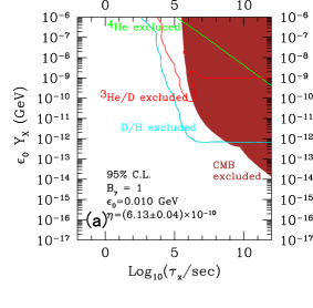
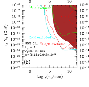
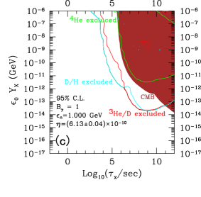
Figure 4: Upper bounds on $\epsilon_{0}Y_{X}$ at 95$\%$ C.L. as a function of lifetime for the energy of a high-energy injected photon, (a) $\epsilon_{0}=10^{-2}$ GeV, (b) $10^{-1}$ GeV, (c) 1 GeV and (d) $10\ {\rm GeV}$. We executed Monte Carlo runs. The lines denote the bounds from ³He/D (red), Y_p (green), D/H (cyan), and the $\mu$- and y-distortion of CMB (brown), respectively.

5.2 Injections of a high-energy line electron

Next, we study the case of a high-energy electron injection. In Fig. 5, we show the upper bounds on $\epsilon_{0}Y_{X}$ as functions of the lifetime of the unstable particle. As we can see, when the injection energy is high enough (i.e, $\epsilon_{0}\gtrsim O(100)\ {\rm MeV}$), the upper bounds on $\epsilon_{0}Y_{X}$ are almost unchanged from those for the case of the high energy photon injection; for such case, the photon spectrum is mostly determined by the total amount of the injected energy in the form of electromagnetic particles, and hence the bounds are insensitive to the species of the injected particles (i.e., $\gamma$ or $e^{\pm}$). For a smaller injection energy, on the contrary, the constraint becomes weaker compared to the case of the high-energy photon injection in particular when the lifetime is relatively long. This is due to the suppression of the photon spectrum for the case where the electromagnetic shower is mainly initiated by the FSR photons (see Section 3). We also note here that the CMB constraint becomes stronger than the BBN constraint for a long lifetime. In particular, for the injection energy lower than the threshold of the ⁴He dissociation, the CMB distortion gives more stringent constraint for $\tau_{X}\gtrsim 10^{7}\ {\rm sec}$.

For comparison, in Fig. 6, we show how the constraints behave if we neglect the effects of FSR, taking $\epsilon_{0}=10$ and $100\ {\rm MeV}$. (We have checked that the constraints are almost unchanged for $\epsilon_{0}\gtrsim 1\ {\rm GeV}$.) We can see that the BBN constraint is weakened for $\epsilon_{0}=100\ {\rm MeV}$ when the lifetime is longer than $\sim 10^{8}\ {\rm sec}$. For the case of $\epsilon_{0}=10\ {\rm MeV}$, the BBN constraints become weaker for $\tau_{X}\gtrsim 10^{6}\ {\rm sec}$. However, for longer lifetime, the constraints becomes almost unchanged even if we neglect the effects of FSR. This is due to the fact that, for such a parameter region, the BBN constraint comes mainly from the change of the baryon-to-photon ratio due to the dilution. As discussed in Section 4, the emission of the electromagnetic particle due to the decaying $X$ induces entropy production which affects the value of the baryon-to-photon ratio. Thus, with the present value of $\eta$ being fixed as Eq. (2.5), the baryon-to-photon ratio at the time of the BBN epoch is larger than it when the effect of the entropy production is significant. The light element abundances are sensitive to the value of $\eta$, and also the BBN calculation based on the value of $\eta$ given in Eq. (2.5). Because the theoretical values of light element abundances are more or less consistent with observed values, the parameter regions, in which large entropy production is induced, are excluded by the observations. The FSR does not affect such a constraint, which is the reason why the constraints become insensitive to the inclusion of the FSR for $\epsilon_{0}=10\ {\rm MeV}$ and long-enough lifetime. (Notice that this is the case only when $\epsilon_{0}\lesssim 20\ {\rm MeV}$, i.e, the threshold energy of ⁴He.)

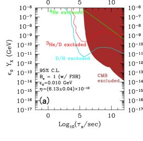
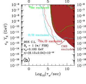
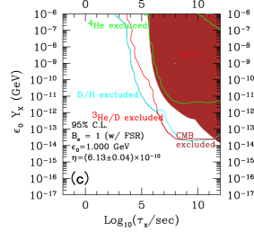
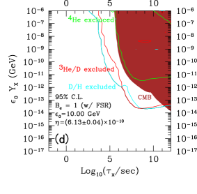
Figure 5: Upper bounds on $\epsilon_{0}Y_{X}$ at 95$\%$ C.L. as a function of lifetime $\tau_{X}$ for the energy of a high-energy injected electron, (a) $\epsilon_{0}=10^{-2}$ GeV, (b) $10^{-1}$ GeV, (c) 1 GeV and (d) $10\ {\rm GeV}$. Effects of the FSR are included in the calculation of the photon and electron spectrum. We executed Monte Carlo runs. The lines denote the bounds from ³He/D (red), Y_p (green), D/H (cyan), and the $\mu$- and y-distortion of CMB (brown), respectively.

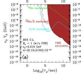
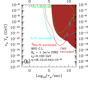
Figure 6: Upper bounds on $\epsilon_{0}Y_{X}$ at 95$\%$ C.L. as a function of lifetime $\tau_{X}$ for the energy of a high-energy injected electron, (a) $\epsilon_{0}=10^{-2}$ and (b) $10^{-1}~{}{\rm GeV}$ omitting effects of the FSR associated with electrons in the final states. We executed Monte Carlo runs. The lines denote the bounds from ³He/D (red), Y_p (green), D/H (cyan), and the $\mu$- and y-distortion of CMB (brown), respectively.

5.3 Comparison with previous works

Here we compare our results with those reported by earlier works on sub-GeV massive particles decaying into electromagnetic daughter particles [25, 26, 27, 28]. Without adopting the universal photon spectrum [4], we have to solve the Boltzmann equations. As shown in Fig. 2 and Fig. 2, our spectra for both the nonthermal photons and electrons are consistent with those in  [27] approximately within a factor of two. Before we directly compare our results with theirs for the bounds on the light element abundances, we remark the following three points.

• We executed the Monte Carlo runs to evaluate theoretical errors of light element abundances. By performing the $\chi^{2}$ analysis using both the theoretical and observational errors, we obtained the upper bounds on $Y_{X}$ as functions of $\tau_{X}$ at 95$\%$ C.L. Because of the Monte Carlo estimation of the theoretical uncertainties, our bounds tend to become milder by a factor of $\sim 2$ than those without the Monte Carlo estimation.

• As for the observational bound on the primordial value of ³He, we adopted the upper bound on ³He/D [34]. On the other hand, the authors in Refs. [25, 26, 27, 28] adopted the observational bound on ³He/H. We believe an upper bound on the primordial value of ³He obtained from ³He/D is more reasonable and conservative than that obtained from ³He/H [33, 6]. That is because the primordial ³He can be destroyed in relatively small stars [65, 66]; it is highly uncertain to estimate how much ³He is destroyed in such stars (see also discussions in [67]). When we consider both destruction and production processes of ³He in stars, it is remarkable that the ratio ³He/D simply increases as a function of the cosmic time through chemical evolutions because D is more fragile than ³He and is destroyed whenever ³He is destroyed. The upper bound on ³He/D shown in (2.2) gives a milder bound on $Y_{X}$ than that from ³He/H $<(1.0\pm 0.5)\times 10^{-5}$ [27, 34], approximately at most by a factor of $\sim 4$ even without executing the Monte Carlo estimation.

• We took into account a dilution of baryon by the entropy production due to the decay of $X$. In our analysis, as an initial condition well before X starts to decay, we took a larger initial value of $\eta$ to realize the present value given in (2.5). At around top-right regions in Figs. 4 – 8, the light element abundances are calculated with the initial value of $\eta$ significantly larger than the value given in (2.5), which gives some difference between ours and the analyses without such modifications on $\eta$.

By considering the above three points, our constraints are consistent with those in  [25, 26, 27] approximately within a factor of two. On the other hand, compared with the results in Ref. [28], it seems that deviations are somehow much larger for the injections of the lower energy photon ($\epsilon_{0}\lesssim$10 MeV).

6 Implication to the ⁷Li Problem

So far, we have neglected the ⁷Li abundance in deriving the upper bounds on the primordial abundance of the unstable particle. This is because, conservatively, the primordial abundance of ⁷Li is still controversial as we have mentioned in Section 2. If the Spite plateau value of ⁷Li really indicates its primordial abundance, it is highly inconsistent with the SBBN prediction, i.e., the ⁷Li problem. It is notable, however, that a long-lived particles decaying into photons may solve difficulty [53, 25]. In this section, we assume that the Spite plateau value (2.4) corresponds to the primordial abundance of ⁷Li and discuss how the decaying particle may solve the ⁷Li problem.

Because the SBBN abundance of ⁷Li given in Eq. (2.4) is about three times larger than the observed value, the ⁷Li problem may be solved if the dissociation processes induced by the radiatively decaying particles reduce right amount of ⁷Li. For the value of baryon-to-photon ratio suggested by the Planck collaboration (see Eq. (2.5)), the ⁷Li in the present Universe mostly originate from ⁷Be which decays into ⁷Li via the electron capture in the SBBN. Thus, if a significant amount of ⁷Be is dissociated by energetic photons emitted by the decay of $X$, the predicted value of the ⁷Li in the present Universe may become consistent with the observed value. In order for such a solution to work, it should be also guaranteed that the emitted photons to dissociate ⁷Be (and ⁷Li) should not cause any harmful effects, i.e., dissociations of other light elements or distortion of the CMB background.

Importantly, the threshold energy of the photon for the process ${\rm{}^{7}Be}(\gamma,{\rm{}^{3}He}){\rm{}^{4}He}$ is $E^{\rm(th)}_{\rm{}^{7}Be}\simeq 1.59\ {\rm MeV}$, which is lower than that of the photodissociation of D ($E^{\rm(th)}_{\rm D}\simeq 2.22\ {\rm MeV}$) and ⁴He ($\sim 20\ {\rm MeV}$). Thus, if the energy of the injected photons is in the range of $E^{\rm(th)}_{\rm{}^{7}Be}<\epsilon_{0}<E^{\rm(th)}_{\rm D}$, the photodissociation of ⁷Be may occur to solve the ⁷Li problem without significantly affecting the abundances of other light elements, as mentioned in [53, 25].

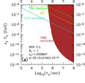
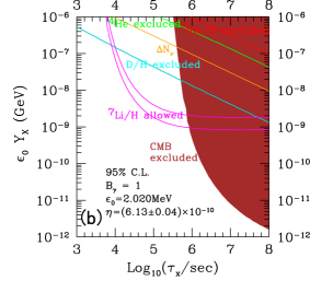
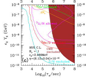
Figure 7: Allowed regions on $\epsilon_{0}Y_{X}$ as a function of lifetime ($\tau_{X}$) to fit ⁷Li/H (magenta) for the energy of a high-energy injected photon, (a) $\epsilon_{0}=1.5~{}{\rm MeV}$, (b) $2.0~{}{\rm MeV}$, and (c) $2.5~{}{\rm MeV}$. We executed Monte Carlo runs.The lines denote the bounds from ³He/D (red), Y_p (green), D/H (cyan), and the $\mu$- and y-distortion of CMB (brown), respectively.

To see if this scenario really works, we calculate the light element abundances for the case of monochromatic photon injection with $\epsilon_{0}=1.5$, $2.0$, and $2.5\ {\rm MeV}$. The results are shown in Fig. 7. For $\epsilon_{0}=1.5\ {\rm MeV}$, the energy of the injected photon is lower than the thresholds of all the photodissociation processes. Then, the constraints are from the entropy production due to the $X$ decay which causes the change of the baryon-to-photon ratio as well as the CMB distortion. Taking $\epsilon_{0}=2\ {\rm MeV}$, on the contrary, the photodissociation of ⁷Be can occur. In this case, we can see that there shows up a parameter region which gives the ⁷Li abundance consistent with Eq. (2.4) without too much affecting the abundances of other light elements. For $\tau_{X}\gtrsim 2\times 10^{6}\ {\rm sec}$, the constraint from the CMB distortion excludes the parameter region of our interest. The CMB constraint is, however irrelevant for shorter lifetime. Consequent, for $8\times 10^{3}\lesssim\tau_{X}\lesssim 2\times 10^{6}\ {\rm sec}$, we can find a parameter region giving the ⁷Li abundance consistent with Eq. (2.4) without conflicting the other constraints. Here, we remark that the photodissociation process in this case is mainly induced by the photons just after the injection, i.e., photons with the energy of $\epsilon_{0}$. Photons after experiencing the electromagnetic shower processes, i.e., cannot effectively induce the photodissociation process when $\epsilon_{0}$ is close to the threshold energy. With the photon energy larger than $E^{\rm(th)}_{\rm D}$, the photodissociation of D occurs as well as the that of ⁷Be. A few % change of the D abundance due to the photodissociation results in a disagreement with the observed value because the observational value of the D abundance is so precise, while about $60-70\ \%$ of ⁷Be should be photodissociated to solve the ⁷Li problem. Because the photodissociation cross sections for these processes are of the same order of magnitude, the D constraint excludes the parameter region which gives right ⁷Be abundance, as indicated in the figure.

For comparison, we also calculate the light element abundances for the case of a monochromatic $e^{\pm}$ injection. For the case of the electron injection with $\epsilon_{0}\sim O(1)\ {\rm MeV}$, the photodissociations are mostly induced by photons emitted by the FSR. Such photon flux is not monochromatic, and is suppressed compared to that in the case of monochromatic photon injection. Consequently, in the case of monochromatic $e^{\pm}$ injection, the ⁷Li problem is hardly solved without conflicting the other constraints.

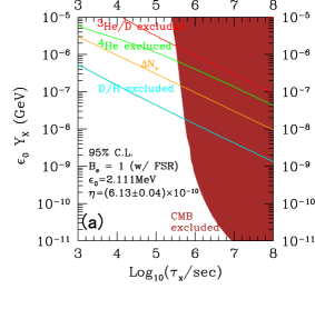
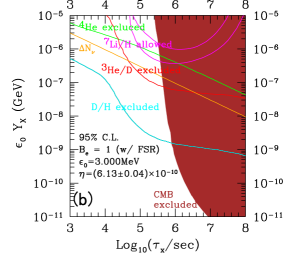
Figure 8: Allowed regions on $\epsilon_{0}Y_{X}$ as a function of lifetime ($\tau_{X}$) to fit ⁷Li/H (magenta) for the energy of a high-energy injected electron, (a) $\epsilon_{0}=2.1~{}{\rm MeV}$, and (b) $3.0~{}{\rm MeV}$ including effects of the FSR associated with electrons in the final states. We executed Monte Carlo runs to obtain theoretical errors of light element abundances. The lines denote the bounds at 95$\%$ C.L. from ³He/D (red), Y_p (green), D/H (cyan), and the $\mu$- and y-distortion of CMB (brown), respectively.

7 Conclusions and Discussion

In this paper, we have studied the effects of the injections of energetic electromagnetic particles (i.e., $\gamma$ and $e^{\pm}$), paying particular attention to the case that the injection energy is sub-GeV. Once the energetic electromagnetic particles are injected into the thermal bath in the early Universe, they induce electromagnetic showers in which energetic photons are copiously produced. If it happens at a cosmic time later than $\sim 1\ {\rm sec}$, such energetic photons in the shower may dissociate the light elements (i.e., D, ³He, ⁴He, and so on), resulting in the change of the predictions of the SBBN. Because the predictions of the SBBN more or less agree with the observations of the primordial abundances of light elements, the injections of the energetic particles in such an epoch is dangerous, and we can obtain an upper bound on the total amount of the injection in order not to spoil the success of the SBBN.

We have concentrated on a long-lived particle $X$ which decays into a pair of photon or $e^{\pm}$, and derived an upper bound on its primordial abundance (Thus, the injection energy is monochromatic if we neglect the FSR). When the injection energy is higher than $\sim 1\ {\rm GeV}$, it has been known that the resultant photon and $e^{\pm}$ spectra in the electromagnetic shower are mostly determined by the total amount of energy injection. For a lower injection energy, on the contrary, the spectra depends on the primary particle injected and the injection energy, as was pointed out by [25, 26, 27].

In our analyses, we have first solved the Boltzmann equations to derive the distributions of photon and $e^{\pm}$ in the electromagnetic shower. The photon spectrum is convoluted with the photodissociation cross sections of light elements to calculate the dissociation rates. Effects of the photodissociations, based on the rates mentioned above, are implemented into a numerical code to follow the evolutions of the light elements with taking into account the effects of photodissociations induced by the injection of energetic $\gamma$ or $e^{\pm}$. The theoretical predictions about the light element abundances are compared with the latest observational constraints to derive upper bound on the primordial abundance of the long-lived particle.

When the injection energy $\epsilon_{0}$ is high enough ($\epsilon_{0}\gtrsim 1\ {\rm GeV}$), the upper bound on the combination of $\epsilon_{0}Y_{X}$ is insensitive to the primary particle injected and the injection energy. For smaller injection energy (i.e., $\epsilon_{0}\lesssim 100\ {\rm MeV}$), on the contrary, the upper bounds become dependent on those injection energies. For smaller $\epsilon_{0}$, the upper bounds on $\epsilon_{0}Y_{X}$ is weaker than those for $\epsilon_{0}\gtrsim 1\ {\rm GeV}$; this is because, for small $\epsilon_{0}$, energy transfer from the energetic particle to the scattered particle (which originally belongs to the thermal bath) becomes inefficient.

We have also discussed the effects of the injection of the electromagnetic particles on the ⁷Li abundance and discussed the implication to the so-called ⁷Li problem. If we regard the Spike-plateau value of the ⁷Li abundance as the primordial value, the SBBN overproduces the ⁷Li abundance by the factor of $\sim 3$. If the energetic particle injected into the thermal bath can selectively dissociate ⁷Be, which is the dominant source of ⁷Li for the value of the baryon-to-photon ratio observed by CMB, the resultant abundance of ⁷Li can be reduced to be consistent with the Spike-plateau value. In Fig.7 (c), we have shown that there really exists a parameter region in which the theoretical prediction of the ⁷Li abundance becomes consistent with the Spike-plateau value without conflicting other constraints; this is particularly due to the smallness of the threshold energy of the ⁷Be.

In this paper, we have performed a general analysis to study the effects of the injections of sub-GeV electromagnetic on the BBN. In particular, we have considered the simplest case that the injection energy is assumed to be monochromatic, treating the lifetime and injection energy (or the mass of the $X$) to be free parameters. Our analysis can be easily applied to models containing a long-lived unstable particle with its mass of sub-GeV. In particular, in some class of models of sub-GeV dark matter, this is the case. One example is the so-called Twin-SIMPs model, in which strongly interacting massive particles (SIMPs) provide a dark matter candidate [24]. In this model, there show up various bound states, whose masses are sub-GeV, due to the newly introduced QCD-like strong interaction. The lightest “meson” becomes the dark matter candidate, while other “mesons” may decay into standard model particles with lifetime longer than $1\ {\rm sec}$. Because the “mesons” are expected to be produced in the thermal bath in the early Universe, some of them may play the role of $X$ in our discussion and affect the light element abundances. In the Twin-SIMPs model, the unstable “mesons” may decay into three or more final states so that the decay products are not monochromatic in general. Thus a dedicated analysis for the Twin-SIMPs model is required to understand possible BBN constraints on the model. Such a study is beyond the scope of this paper, and will be given elsewhere [68].

Appendix A Analytical Formula of the Dilution Factor

Here we discuss the analytical formula of the dilution factor induced by the late-time entropy production due to radiatively decaying particles. For simplicity, we assume that the parent particle (called $X$) decays into photons instantaneously with the increase of the photon energy density $\Delta\rho_{\gamma}$ at a cosmic time $t=\tau_{X}$ where $\tau_{X}$ is the lifetime of $X$. In addition, we assume that the emitted photons are immediately thermalized to be a black body distribution. Then, we can approximately estimate the dilution factor as

$$\Delta_{\rm dilution}=1+\frac{\Delta s}{s}=\left(\frac{T_{a}}{T_{b}}\right)^{3},$$ (A.1)

where $T_{a}$ and $T_{b}$ are the photon temperature just after and just before the entropy production, respectively. Here $\Delta s$ is the increase of the entropy density. On the other hand, $\Delta\rho_{\gamma}$ is related with $T_{a}/T_{b}$ by

$$\frac{\rho_{\gamma}+\Delta\rho_{\gamma}}{\rho_{\gamma}}=\left(\frac{T_{a}}{T_{b}}\right)^{4}.$$ (A.2)

From Eqs. (A.1) and (A.2), we have

$$\Delta_{\rm dilution}=\left(1+\frac{\Delta\rho_{\gamma}}{\rho_{\gamma}}\right)^{3/4}.$$ (A.3)

Hereafter we consider only the entropy production after the $e^{+}e^{-}$–annihilation epoch, i.e., $T\lesssim 1{\rm MeV}$. Although this assumption is not correct for shorter lifetime in general, you will find later that it is reasonable in the parameter regions for the current interests. Using the relation $s=7.04n_{\gamma}$ between the entropy density $s$ and the number density of photon $n_{\gamma}$, we obtain

$$\frac{\Delta\rho_{\gamma}}{\rho_{\gamma}}=\frac{7.04}{2.701}\frac{1}{T}\frac{\Delta\rho_{\gamma}}{s},$$ (A.4)

where we used $\rho_{\gamma}=2.701Tn_{\gamma}$.

From the Friedmann equation, the temperature at $t=\tau_{X}$ is approximately expressed by

$$T=1.556\times 10^{-3}{\rm GeV}g_{*}^{-1/4}\left(\frac{\tau_{X}}{{\rm sec}}\right)^{-1/2},$$ (A.5)

with the statistical degree of freedom,

$$g_{*}=3.363+2\frac{\Delta\rho_{\gamma}}{\rho_{\gamma}}.$$ (A.6)

By substituting Eq. (A.5) into Eq. (A.4), we have a quartic equation for $x=\Delta\rho_{\gamma}/{\rho_{\gamma}}$,

$$A^{4}x^{4}-2C^{4}x-C^{4}B=0,$$ (A.7)

with

$$A=0.5970\times 10^{-3}\left(\frac{\tau_{X}}{\rm sec}\right)^{-1/2},\quad B=3.363,\quad C=\left(\frac{\Delta\rho_{\gamma}/s}{\rm GeV}\right).$$ (A.8)

The exact solution for a positive real number of $x$ is analytically represented by

$$x=\Delta\rho_{\gamma}/{\rho_{\gamma}}=\frac{C}{2}\left(\sqrt{D}+\sqrt{-D+\frac{4C}{A^{4}}\frac{1}{\sqrt{D}}}\right)$$ (A.9)

where

$$D=2^{1/3}3^{-2/3}A^{-8/3}F-2^{5/3}3^{-1/3}A^{-4/3}B/F,$$ (A.10)

with

$$F=\left(9C^{2}+\sqrt{3}\sqrt{16A^{4}B^{3}+27C^{4}}\right)^{1/3}.$$ (A.11)

By using this solution, we can calculate $\Delta_{\rm dilution}$ through Eq. (A.3).

In Fig. 9 we plot the contours of the dilution factor $\Delta_{\rm dilution}$ in the $\tau_{X}$ – $\Delta\rho_{\gamma}/s$ plane. The solid lines are the results of the numerical computation. The dotted lines are the analytical formula given in Eqs. (A.3) and (A.9). From this figure, we see that the analytical formula fits the numerical results very well. In this parameter space, the meaningful entropy production occurs for $\tau_{X}\gtrsim 1{\rm sec}$, which corresponds to the decay epoch $T\lesssim 1{\rm MeV}$. Therefore the assumption to derive Eq. (A.9) that we considered only the relationship among the physical variables after the $e^{+}e^{-}$–annihilation is reasonable.

Because the exact solution in Eq. (A.9) is little bit complicated, it might be useful to give a simpler approximate solution. When we join the solutions for both the limit cases of $C=\Delta\rho_{\gamma}/s/{\rm GeV}\to\infty$ and $C\to 0$, we obtain

$$\Delta\rho_{\gamma}/\rho_{\gamma}=\left\{\begin{array}[]{ll}\displaystyle{\frac{B^{1/4}}{A}C}&~{}~{}:~{}~{}\displaystyle{C\leq\frac{1}{2}AB^{3/4}}\\ \\ \displaystyle{2^{1/3}\left(\frac{C}{A}\right)^{4/3}}&~{}~{}:~{}~{}\displaystyle{C>\frac{1}{2}AB^{3/4}}\end{array}\right..$$ (A.15)

This simple formula also agrees with the exact solution within the precision of O(1) $\%$ for $\Delta_{\rm dilution}\ll{\cal O}(10)$.

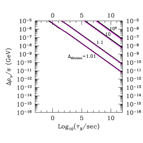
Figure 9: Contours of the dilution factor $\Delta_{\rm dilution}$ in the $\tau_{X}$ – $\Delta\rho_{\gamma}/s$ plane. The solid lines represent the results of the numerical computation. The dotted lines are the analytical solutions which are given in Eqs. (A.3) and  (A.9).

Appendix B Final State Radiation

In this appendix, we derive the formulae for the rate of a decay process with a FSR photon under some assumptions.

First, we consider the process in which two ultra-relativistic electron-positron pairs are emitted and compare the decay rate of the process with a FSR photon and that without FSR photons. The diagrams to be considered are shown in Fig. 11, 11.

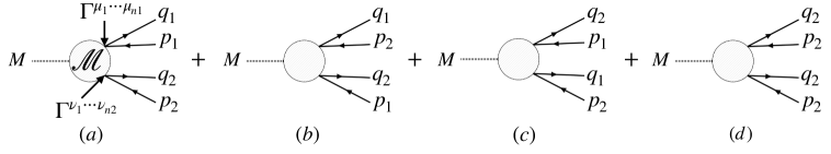
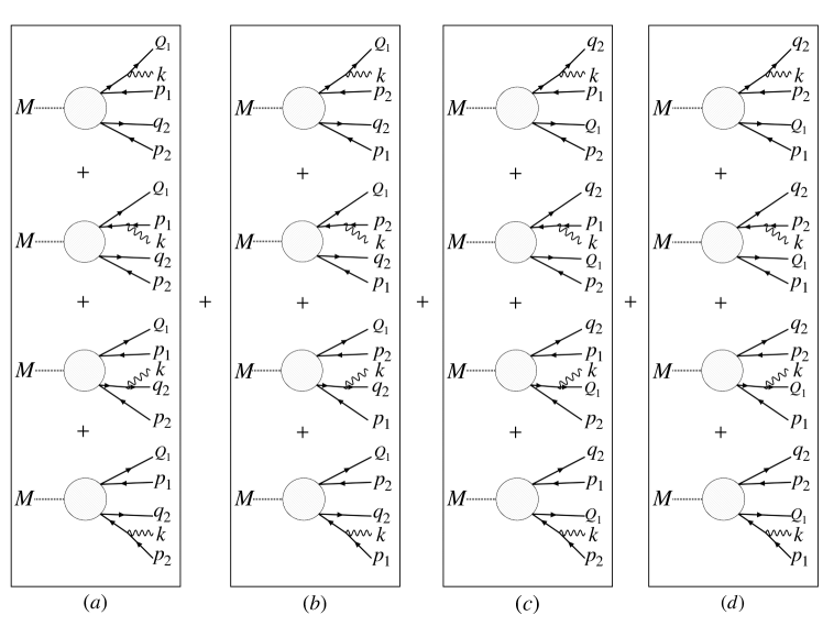
Figure 10: The diagrams without the FSR.

Figure 11: The diagram with the FSR.

In Fig. 11, 11, $\Gamma_{1}^{\mu_{1}\cdots\mu_{n_{1}}}\Gamma_{2}^{\nu_{1}\cdots\nu_{n_{2}}}\mathcal{M}_{\mu_{1}\cdots\mu_{n_{1}}\nu_{1}\cdots\nu_{n_{2}}}$ represents the contribution from the shaded circle, and $\Gamma_{1}^{\mu_{1}\cdots\mu_{n_{1}}}$ and $\Gamma_{2}^{\nu_{1}\cdots\nu_{n_{2}}}$ represent products of gamma matrices which couple to one electron-positron pair and the other pair, respectively. Here, we assume the momentum dependence of $\mathcal{M}$ is $\mathcal{M}_{\mu_{1}\cdots\mu_{n_{1}}\nu_{1}\cdots\nu_{n_{2}}}(q_{1}+p_{1},q_{2}+p_{2})$ for the diagram shown in Fig. 11(a). We assume the similar momentum dependences for the other diagrams in Fig. 11. Under this assumption, the upper half diagrams in Fig. 11(a) have $\mathcal{M}_{\mu_{1}\cdots\mu_{n_{1}}\nu_{1}\cdots\nu_{n_{2}}}(Q_{1}+p_{1}+k,q_{2}+p_{2})$ and the lower half diagrams have $\mathcal{M}_{\mu_{1}\cdots\mu_{n_{1}}\nu_{1}\cdots\nu_{n_{2}}}(Q_{1}+p_{1},q_{2}+p_{2}+k)$. In addition, we assume each final state particle is ultra-relativistic.

Before calculating the decay rates, let us observe the diagrams with a FSR photon and determine which terms of the matrix element are dominant. Comparing the diagrams with a FSR photon with those without FSR photons, the matrix element of the process with a FSR photon has one additional propagator of electron. For example, Fig. 11(a) has

$$\frac{i(\cancel{Q}_{1}+\cancel{k}+m_{e})}{(Q_{1}+k)^{2}-m_{e}^{2}}=\frac{i(\cancel{Q}_{1}+\cancel{k}+m_{e})}{2k\cdot Q_{1}}.$$ (B.1)

Since we assumed that each electron and positron is ultra-relativistic, the denominator is small when $k$ and $Q_{1}$ are collinear. This is also the case with a FSR photon emitted from a positron. Therefore, we can consider the cross section is dominated by the process in which the FSR photon is collinear with one of electrons or positrons. Based on this observation, we proceed with the calculation for the FSR photon collinear with $Q_{1}$.

In general, the decay rate of a massive particle with mass $M$ is written as

$$\mathrm{d}\Gamma=\frac{1}{2M}\left(\prod_{\mathrm{f}}\frac{\mathrm{d}^{3}p_{\mathrm{f}}}{(2\pi)^{3}2p^{0}_{\mathrm{f}}}\right)\sum_{\mathrm{spin,polarization}}\Big{|}\mathcal{M}\left(M\to\{p_{\mathrm{f}}\}\right)\Big{|}^{2}(2\pi)^{4}\delta^{4}\left(\sum_{\mathrm{f}}p_{\mathrm{f}}-M\right),$$ (B.2)

where $p_{\mathrm{f}}$ is the momentum of final state particles and we abbreviated $(M,\vec{0})$ as $M$. In the case of Fig. 11, the decay rate $\Gamma_{1\to 4}$ is

$$\mathrm{d}\Gamma_{1\to 4}= \frac{1}{2M}\frac{\mathrm{d}^{3}q_{1}}{(2\pi)^{3}2q_{1}^{0}}\frac{\mathrm{d}^{3}q_{2}\mathrm{d}^{3}p_{1}\mathrm{d}^{3}p_{2}}{8(2\pi)^{9}q_{2}^{0}p_{1}^{0}p_{2}^{0}}$$

$$\times\sum_{\mathrm{spin}}\Big{|}\mathcal{M}_{1\to 4}\left(q_{1},q_{2};p_{1},p_{2}\right)\Big{|}^{2}(2\pi)^{4}\delta^{4}\left(\sum_{\mathrm{f}}p_{\mathrm{f}}-M\right),$$ (B.3)

where the matrix element is $\mathcal{M}_{1\to 4}$. In the case of Fig. 11, the decay rate $\Gamma_{1\to 5}$ is

$$\mathrm{d}\Gamma_{1\to 5}= \frac{1}{2M}\frac{\mathrm{d}^{3}k\mathrm{d}^{3}Q_{1}}{(2\pi)^{6}2k^{0}2Q_{1}^{0}}\frac{\mathrm{d}^{3}q_{2}\mathrm{d}^{3}p_{1}\mathrm{d}^{3}p_{2}}{8(2\pi)^{9}q_{2}^{0}p_{1}^{0}p_{2}^{0}}$$

$$\times\sum_{\mathrm{spin,polar}}\Big{|}\mathcal{M}_{1\to 5}\left(k;Q_{1},q_{2};p_{1},p_{2}\right)\Big{|}^{2}(2\pi)^{4}\delta^{4}\left(\sum_{\mathrm{f}}p_{\mathrm{f}}-M\right),$$ (B.4)

where the matrix element is $\mathcal{M}_{1\to 5}$. Considering the electron is ultra-relativistic,

$$\mathrm{d}^{3}k\mathrm{d}^{3}Q_{1}\simeq\mathrm{d}k^{0}\mathrm{d}Q^{0}_{1}\mathrm{d}\Omega_{k}\mathrm{d}\Omega_{Q_{1}}(k^{0})^{2}(Q_{1}^{0})^{2}.$$ (B.5)

From the above observation, we integrate in the interval,

$$0\leq\theta\leq\theta_{0}\quad,\quad\frac{m}{q_{1}^{0}}\ll\theta_{0}\ll 1,$$ (B.6)

where $\theta$ is the angle between $\vec{k}$ and $\vec{Q_{1}}$. This interval is sufficiently collinear and contains the region in which the integrand is not negligible. In the collinear region, we can perform a change of variables such as

$$\begin{split}k^{0}&=xq_{1}^{0},\\ Q_{1}^{0}&=(1-x)q_{1}^{0}.\end{split}$$ (B.7)

Therefore, we obtain

$$\begin{split}k^{\mu}&=xq_{1}^{0}(1,\hat{k}),\\ Q_{1}^{\mu}&=(1-x)q_{1}^{0}(1,v\hat{Q}_{1}),\end{split}$$ (B.8)

where, from the on-shell condition of the electron,

$$(Q_{1})^{2}=m_{e}^{2} =(1-x)^{2}\left(q_{1}^{0}\right)^{2}(1-v^{2})$$

$$\sim 2(1-x)^{2}\left(q_{1}^{0}\right)^{2}(1-v)\quad(\mathrm{except\,for}\,x\sim 1).$$ (B.9)

That is

$$1-v\sim\frac{m_{e}^{2}}{2(1-x)^{2}\left(q^{0}_{1}\right)^{2}}\quad(\mathrm{except\,for}\,x\sim 1).$$ (B.10)

For the change of variables (B.7),

$$\left|\begin{array}[]{rr}\frac{\partial{k^{0}}}{\partial x}&\frac{\partial{Q_{1}^{0}}}{\partial x}\\ \frac{\partial{k^{0}}}{\partial q_{1}^{0}}&\frac{\partial{Q_{1}^{0}}}{\partial q_{1}^{0}}\end{array}\right|=\left|\begin{array}[]{rr}q_{1}^{0}&-q_{1}^{0}\\ x&1-x\end{array}\right|=q_{1}^{0},$$

which leads to

$$\mathrm{d}k^{0}\mathrm{d}Q^{0}_{1}=q_{1}^{0}\mathrm{d}x\mathrm{d}q_{1}^{0}.$$ (B.11)

From Eq. (B.11)

$$\frac{\mathrm{d}^{3}k\mathrm{d}^{3}Q_{1}}{(2\pi)^{6}2k^{0}2Q_{1}^{0}} =\frac{\mathrm{d}^{3}q_{1}}{(2\pi)^{3}2q_{1}^{0}}\mathrm{d}x\mathrm{d}(\cos{\theta})\frac{x(1-x)}{8\pi^{2}}\left(q_{1}^{0}\right)^{2},$$ (B.12)

where, in the second equality, we changed the variables from $\vec{k}$ and $\vec{Q_{1}}$ to $\vec{q_{1}}$ and the angle between $\vec{k}$ and $\vec{Q_{1}}$. Here, we assumed the integrand does not depend on the azimuthal angle between $\vec{k}$ and $\vec{Q_{1}}$. As seen below, this assumption is justified in the case concerned. Using Eq. (B.12) we obtain

$$\mathrm{d}\Gamma_{1\to 5}= \frac{1}{2M}\frac{\mathrm{d}^{3}q_{1}}{(2\pi)^{3}2q_{1}^{0}}\frac{\mathrm{d}^{3}q_{2}\mathrm{d}^{3}p_{1}\mathrm{d}^{3}p_{2}}{8(2\pi)^{9}q_{2}^{0}p_{1}^{0}p_{2}^{0}}\mathrm{d}x\mathrm{d}(\cos{\theta})\frac{x(1-x)}{8\pi^{2}}\left(q_{1}^{0}\right)^{2}$$

$$\times\sum_{\mathrm{spin,polar}}\Big{|}\mathcal{M}_{1\to 5}\left(k;Q_{1},q_{2};p_{1},p_{2}\right)\Big{|}^{2}(2\pi)^{4}\delta^{4}\left(\sum_{\mathrm{f}}p_{\mathrm{f}}-M\right).$$ (B.13)

Corresponding to the four diagrams (a)-(d) in Fig.11 $\mathcal{M}_{1\to 4}$ is written as

$$\mathcal{M}_{1\to 4}=\mathcal{M}_{1\to 4}^{(a)}+\mathcal{M}_{1\to 4}^{(b)}+\mathcal{M}_{1\to 4}^{(c)}+\mathcal{M}_{1\to 4}^{(d)}.$$ (B.14)

$\mathcal{M}_{1\to 5}$ is written in the same way. $\mathcal{M}^{(i)}_{1\to 4}(i=a,\ldots,d)$ are given by

$$i\mathcal{M}_{1\to 4}^{(a)} =i\mathcal{M}_{\mu\nu}\mathrm{bar}{u}^{s_{1}}(q_{1})\Gamma^{\mu}_{1}v^{s^{\prime}_{1}}(p_{1})\mathrm{bar}{u}^{s_{2}}(q_{2})\Gamma^{\nu}_{2}v^{s^{\prime}_{2}}(p_{2}),$$ (B.15)

$$i\mathcal{M}_{1\to 4}^{(b)} =i\mathcal{M}_{\mu\nu}\mathrm{bar}{u}^{s_{1}}(q_{1})\Gamma^{\mu}_{1}v^{s^{\prime}_{2}}(p_{2})\mathrm{bar}{u}^{s_{2}}(q_{2})\Gamma^{\nu}_{2}v^{s^{\prime}_{1}}(p_{1}),$$ (B.16)

$$i\mathcal{M}_{1\to 4}^{(c)} =i\mathcal{M}_{\mu\nu}\mathrm{bar}{u}^{s_{2}}(q_{2})\Gamma^{\mu}_{1}v^{s^{\prime}_{1}}(p_{1})\mathrm{bar}{u}^{s_{1}}(q_{1})\Gamma^{\nu}_{2}v^{s^{\prime}_{2}}(p_{2}),$$ (B.17)

$$i\mathcal{M}_{1\to 4}^{(d)} =i\mathcal{M}_{\mu\nu}\mathrm{bar}{u}^{s_{2}}(q_{2})\Gamma^{\mu}_{1}v^{s^{\prime}_{2}}(p_{2})\mathrm{bar}{u}^{s_{1}}(q_{1})\Gamma^{\nu}_{2}v^{s^{\prime}_{1}}(p_{1}),$$ (B.18)

where we abbreviated $\mu_{1},\cdots,\mu_{n_{1}},\nu_{1},\cdots,\nu_{n_{2}}$ as $\mu,\nu$. Each of $\mathcal{M}^{(i)}_{1\to 5}$ has four terms due to the four possible insertion of a FSR photon to the external lines of the corresponding diagram in Fig. 11. For example,

$$\begin{split}i\mathcal{M}_{1\to 5}^{(a)}=i\mathcal{M}_{\mu\nu}e\varepsilon^{*}_{\alpha}(k)\biggl{[}&\mathrm{bar}{u}^{s_{1}}(Q_{1})\gamma^{\alpha}\frac{\cancel{Q}_{1}+\cancel{k}}{2k\cdot Q_{1}}\Gamma^{\mu}_{1}v^{s^{\prime}_{1}}(p_{1})\mathrm{bar}{u}^{s_{2}}(q_{2})\Gamma^{\nu}_{2}v^{s^{\prime}_{2}}(p_{2})\\ +&\mathrm{bar}{u}^{s_{1}}(Q_{1})\Gamma^{\mu}_{1}\frac{-\cancel{p}_{1}-\cancel{k}}{2k\cdot p_{1}}\gamma^{\alpha}v^{s^{\prime}_{1}}(p_{1})\mathrm{bar}{u}^{s_{2}}(q_{2})\Gamma^{\nu}_{2}v^{s^{\prime}_{2}}(p_{2})\\ +&\mathrm{bar}{u}^{s_{1}}(Q_{1})\Gamma^{\mu}_{1}v^{s^{\prime}_{1}}(p_{1})\mathrm{bar}{u}^{s_{2}}(q_{2})\gamma^{\alpha}\frac{\cancel{q}_{2}+\cancel{k}}{2k\cdot q_{1}}\Gamma^{\nu}_{2}v^{s^{\prime}_{2}}(p_{2})\\ +&\mathrm{bar}{u}^{s_{1}}(Q_{1})\Gamma^{\mu}_{1}v^{s^{\prime}_{1}}(p_{1})\mathrm{bar}{u}^{s_{2}}(q_{2})\Gamma^{\nu}_{2}\frac{-\cancel{p}_{2}-\cancel{k}}{2k\cdot p_{2}}\gamma^{\alpha}v^{s^{\prime}_{2}}(p_{2})\biggr{]}.\end{split}$$ (B.19)

In the following, first we show

$$\sum_{\mathrm{spin,polar}}\mathcal{M}_{1\to 5}^{(i)}\mathcal{M}_{1\to 5}^{(j)*}=F(x,q^{0}_{1},\theta,v)\sum_{\mathrm{spin}}\mathcal{M}_{1\to 4}^{(i)}\mathcal{M}_{1\to 4}^{(j)*}$$ (B.20)

for all $i,j=a,b,c,d$ using a function $F(x,q^{0}_{1},\theta,v)$. We then can show

$$\sum_{\mathrm{spin,polar}}|\mathcal{M}_{1\to 5}|^{2}=F(x,q^{0}_{1},\theta,v)\sum_{\mathrm{spin}}|\mathcal{M}_{1\to 4}|^{2}.$$ (B.21)

Since $\mathcal{M}_{1\to 5}^{(i)}$ and $\mathcal{M}_{1\to 5}^{(j)*}$ have four terms, $\mathcal{M}_{1\to 5}^{(i)}\mathcal{M}_{1\to 5}^{(j)*}$ has 16 terms. But, as mentioned above, the dominant contribution comes from the term which has $k\cdot Q_{1}$ in the denominator. Therefore, we focus on the 1 term with the product of the propagators proportional to $\propto(k\cdot Q_{1})^{-2}$ and the 6 terms with the product of the propagators proportional to $\propto(k\cdot Q_{1})^{-1}$. $\sum_{\mathrm{spin}}\mathcal{M}_{1\to 4}^{(i)}\mathcal{M}_{1\to 4}^{(j)*}$ can be written as

$$\sum_{\mathrm{spin}}\mathcal{M}_{1\to 4}^{(i)}\mathcal{M}_{1\to 4}^{(j)*}=\mathcal{M}_{\mu_{1}\nu_{1}}\mathcal{M}^{*}_{\mu_{2}\nu_{2}}\mathrm{tr}\left[\cdots\cancel{q}_{1}\cdots\right].$$ (B.22)

Strictly, the RHS is the product of two traces for some $(i,j)$s, but here we ignored the difference because it does not affect the result.
Corresponding to this expression, the term proportional to $\propto(k\cdot Q_{1})^{-2}$ in $\sum\mathcal{M}_{1\to 5}^{(i)}\mathcal{M}_{1\to 5}^{(j)*}$ is

$$\sum_{\mathrm{spin,polar}}\mathcal{M}_{1\to 5}^{(i)}\mathcal{M}_{1\to 5}^{(j)*}\supset-e^{2}\mathcal{M}_{\mu_{1}\mu_{2}}\mathcal{M}^{*}_{\mu_{3}\mu_{4}}\mathrm{tr}\left[\cdots\frac{\cancel{Q}_{1}+\cancel{k}}{2k\cdot Q_{1}}\gamma^{\alpha}\cancel{Q}_{1}\gamma_{\alpha}\frac{\cancel{Q}_{1}+\cancel{k}}{2k\cdot Q_{1}}\cdots\right],$$ (B.23)

where we used $\sum_{\mathrm{polar}}\varepsilon_{\mu}(k)\varepsilon^{*}_{\nu}(k)=-g_{\mu\nu}$ and ignored $m_{e}$ in the propagators because of the ultra-relativisticity of electrons and positrons. In addition, the part denoted by $\cdots$ in the trace is the same in Eqs. (B.22) and (B.23). For the trace part of Eq. (B.23) notice that

$$\frac{\cancel{Q}_{1}+\cancel{k}}{2k\cdot Q_{1}}\gamma^{\alpha}\cancel{Q}_{1}\gamma_{\alpha}\frac{\cancel{Q}_{1}+\cancel{k}}{2k\cdot Q_{1}} =-\frac{x\cancel{q}_{1}}{k\cdot Q_{1}},$$ (B.24)

where we have ignored $m_{e}^{2}$.
Therefore, the contribution from the term proportional to $\propto(k\cdot Q_{1})^{-2}$ is

$$\sum_{\mathrm{spin,polar}}\mathcal{M}_{1\to 5}^{(i)}\mathcal{M}_{1\to 5}^{(j)*}\supset\frac{e^{2}x}{k\cdot Q_{1}}\sum_{\mathrm{spin}}\mathcal{M}_{1\to 4}^{(i)}\mathcal{M}_{1\to 4}^{(j)*}.$$ (B.25)

Next, we consider the 6 terms proportional to $\propto(k\cdot Q_{1})^{-1}$. For example, we focus on the terms whose propagators are proportional to $\propto(k\cdot p_{1}k\cdot Q_{1})^{-1}$.
First, notice that $\sum_{\mathrm{spin}}\mathcal{M}_{1\to 4}^{(i)}\mathcal{M}_{1\to 4}^{(j)*}$ is written in the following form:

$$\sum_{\mathrm{spin}}\mathcal{M}_{1\to 4}^{(i)}\mathcal{M}_{1\to 4}^{(j)*}=\mathcal{M}_{\mu_{1}\mu_{2}}\mathcal{M}^{*}_{\mu_{3}\mu_{4}}\mathrm{tr}\left[\cdots\cancel{q}_{1}\cdots\cancel{p}_{1}\cdots\right].$$ (B.26)

Corresponding to this expression, the term proportional to $\propto(k\cdot p_{1}k\cdot Q_{1})^{-1}$ in $\sum\mathcal{M}_{1\to 5}^{(i)}\mathcal{M}_{1\to 5}^{(j)*}$ is written as

$$\begin{split}\sum_{\mathrm{spin,polar}}\mathcal{M}_{1\to 5}^{(i)}\mathcal{M}_{1\to 5}^{(j)*}\supset-e^{2}\mathcal{M}_{\mu_{1}\mu_{2}}\mathcal{M}^{*}_{\mu_{3}\mu_{4}}\mathrm{tr}\biggl{[}&\cdots\cancel{Q}_{1}\gamma^{\alpha}\frac{\cancel{Q}_{1}+\cancel{k}}{2k\cdot Q_{1}}\cdots\cancel{p}_{1}\gamma_{\alpha}\frac{-\cancel{p}_{1}-\cancel{k}}{2k\cdot p_{1}}\cdots\\ +&\cdots\frac{\cancel{Q}_{1}+\cancel{k}}{2k\cdot Q_{1}}\gamma^{\alpha}\cancel{Q}_{1}\cdots\frac{-\cancel{p}_{1}-\cancel{k}}{2k\cdot p_{1}}\gamma_{\alpha}\cancel{p}_{1}\cdots\biggr{]}.\end{split}$$ (B.27)

In order to keep the leading order, we can ignore $k\cdot Q_{1}$ in the numerator. In other words, we can assume $k\parallel Q_{1}$. Therefore, the first term in the trace of (B.27) is written as

$$\cdots\cancel{Q}_{1}\gamma^{\alpha}\frac{\cancel{Q}_{1}+\cancel{k}}{2k\cdot Q_{1}}\cdots\cancel{p}_{1}\gamma_{\alpha}\frac{-\cancel{p}_{1}-\cancel{k}}{2k\cdot p_{1}}\cdots= \frac{-(1-x)}{xk\cdot Q_{1}}\cdots\cancel{q}_{1}\cdots\cancel{p}_{1}\cdots.$$ (B.28)

The second term in the trace of (B.27) can be transformed in the same way. As a result, the sum of the terms whose propagators are proportional to $(k\cdot p_{1}k\cdot Q_{1})^{-1}$ is

$$\sum_{\mathrm{spin,polar}}\mathcal{M}_{1\to 5}^{(i)}\mathcal{M}_{1\to 5}^{(j)*}\supset\frac{2e^{2}(1-x)}{xk\cdot Q_{1}}\sum_{\mathrm{spin}}\mathcal{M}_{1\to 4}^{(i)}\mathcal{M}_{1\to 4}^{(j)*}.$$ (B.29)

The 2 terms proportional to $\propto(k\cdot p_{2}k\cdot Q_{1})^{-1}$ and the 2 terms proportional to $\propto(k\cdot q_{2}k\cdot Q_{1})^{-1}$ are opposite in sign because of the sign of the propagators. So, they completely cancel. Thus, the contribution from the 6 terms proportional to $\propto(k\cdot Q_{1})^{-1}$ is given by

$$\sum_{\mathrm{spin,polar}}\mathcal{M}_{1\to 5}^{(i)}\mathcal{M}_{1\to 5}^{(j)*} \supset(1+1-1)\frac{2e^{2}(1-x)}{xk\cdot Q_{1}}\sum_{\mathrm{spin}}\mathcal{M}_{1\to 4}^{(i)}\mathcal{M}_{1\to 4}^{(j)*}$$

$$=\frac{2e^{2}(1-x)}{xk\cdot Q_{1}}\sum_{\mathrm{spin}}\mathcal{M}_{1\to 4}^{(i)}\mathcal{M}_{1\to 4}^{(j)*}.$$ (B.30)

Summing all the contributions, we obtain

$$\sum_{\mathrm{spin,polar}}\mathcal{M}_{1\to 5}^{(i)}\mathcal{M}_{1\to 5}^{(j)*} =e^{2}\left(x+\frac{2(1-x)}{x}\right)\frac{1}{k\cdot Q_{1}}\sum_{\mathrm{spin}}\mathcal{M}_{1\to 4}^{(i)}\mathcal{M}_{1\to 4}^{(j)*}+\mathcal{O}\left((k\cdot Q_{1})^{0}\right)$$

$$\simeq e^{2}\frac{1+(1-x)^{2}}{x^{2}(1-x)}\frac{1}{\left(q_{1}^{0}\right)^{2}(1-v\cos{\theta})}\sum_{\mathrm{spin}}\mathcal{M}_{1\to 4}^{(i)}\mathcal{M}_{1\to 4}^{(j)*}.$$ (B.31)

This is exactly the form of (B.20) and we can read $F(x,q_{1}^{0},\theta,v)$ from this expression as

$$\sum_{\mathrm{spin,polar}}\left|\mathcal{M}_{1\to 5}\right|^{2}\simeq e^{2}\frac{1+(1-x)^{2}}{x^{2}(1-x)}\frac{1}{\left(q_{1}^{0}\right)^{2}(1-v\cos{\theta})}\sum_{\mathrm{spin}}\left|\mathcal{M}_{1\to 4}\right|^{2}.$$ (B.32)

Using (B.13) and (B.32), let us compare the decay rate with the FSR and that without FSRs. Note that, because $F(x,q_{1}^{0},\theta,v)$ is independent of the angle between $\vec{k}$ and $\vec{Q_{1}}$, we can use (B.13). When the FSR photon is radiated collinear with the electron $Q_{1}$,

$$\mathrm{d}\Gamma_{1\to 5}\simeq \frac{1}{2M}\frac{\mathrm{d}^{3}q_{1}}{(2\pi)^{3}2q_{1}^{0}}\frac{\mathrm{d}^{3}q_{2}\mathrm{d}^{3}p_{1}\mathrm{d}^{3}p_{2}}{8(2\pi)^{9}q_{2}^{0}p_{1}^{0}p_{2}^{0}}\mathrm{d}x\mathrm{d}(\cos{\theta})\frac{x(1-x)}{8\pi^{2}}\left(q_{1}^{0}\right)^{2}$$

$$\times e^{2}\frac{1+(1-x)^{2}}{x^{2}(1-x)}\frac{1}{\left(q_{1}^{0}\right)^{2}(1-v\cos{\theta})}\sum_{\mathrm{spin}}\left|\mathcal{M}_{1\to 4}\right|^{2}(2\pi)^{4}\delta^{4}\left(\sum p\right)$$

$$= \mathrm{d}x\frac{\alpha}{2\pi}\frac{1+(1-x)^{2}}{x}\log\left[\frac{1-\cos{\theta_{0}}}{1-v}\right]\mathrm{d}\Gamma_{1\to 4}.$$ (B.33)

From (B.10),

$$\frac{\mathrm{d}\Gamma_{1\to 5}}{\mathrm{d}x}(xq_{1};(1-x)q_{1},q_{2};p_{1},p_{2})$$

$$\simeq\frac{\alpha}{2\pi}\frac{1+(1-x)^{2}}{x}\log\left[\frac{2(1-x)^{2}(q_{1}^{0})^{2}(1-\cos{\theta_{0})}}{m_{e}^{2}}\right]\mathrm{d}\Gamma_{1\to 4}(q_{1},q_{2};p_{1},p_{2})$$ (B.34)

except for $x\sim 1$. Here, the arguments of $\frac{\mathrm{d}\Gamma_{1\to 5}}{\mathrm{d}x}$ are the momenta of photon, electrons and positrons from left to right.

In the following part, we will extend this result to the more general case. First, we consider the case where the FSR photon is collinear with a positron. In this case, we only have to change the sign of the propagators, and because we have calculated the product of two propagators in $\sum|\mathcal{M}_{1\to 5}|^{2}$, this does not change the result:

$$\frac{\mathrm{d}\Gamma_{1\to 5}}{\mathrm{d}x}(xp_{1};q_{1},q_{2};(1-x)p_{1},p_{2})$$

$$\simeq\frac{\alpha}{2\pi}\frac{1+(1-x)^{2}}{x}\log\left[\frac{2(1-x)^{2}(p_{1}^{0})^{2}(1-\cos{\theta_{0})}}{m_{e}^{2}}\right]\mathrm{d}\Gamma_{1\to 4}(q_{1},q_{2};p_{1},p_{2}).$$ (B.35)

Second, we consider the case where the final state includes different species of fermion-anti-fermion pairs. In this case, we have to change the classification of the diagrams in Fig. 11 and Fig. 11. However, we have calculated each $\mathcal{M}^{(i)}$ and the same derivation is also applicable in this case. Therefore, the resultant expression is given by (B.10) with the electron mass replaced by that of an appropriate fermion. Third, we consider the case where the final state has $n$ pairs of fermions. In this case, we have to change the calculation from (B.26) to (B.30). Now, we have to calculate $2(2n-1)$ terms instead of 6 terms. But each 4 terms cancel in the same way as the above calculation and we have only the same contribution from 2 terms left. After all, we get the result:

$$\frac{\mathrm{d}\Gamma_{1\to 2n+1}}{\mathrm{d}x}(xq_{1};(1-x)q_{1},q_{2},\cdots,q_{n};p_{1},\cdots,p_{n})$$

$$\simeq\frac{\alpha}{2\pi}\frac{1+(1-x)^{2}}{x}\log\left[\frac{2(1-x)^{2}(q_{1}^{0})^{2}(1-\cos{\theta_{0})}}{m^{2}}\right]\mathrm{d}\Gamma_{1\to 2n}(q_{1},\cdots,q_{n};p_{1},\cdots,p_{n}),$$ (B.36)

$$\frac{\mathrm{d}\Gamma_{1\to 2n+1}}{\mathrm{d}x}(xp_{1};q_{1},\cdots,q_{n};(1-x)p_{1},p_{2},\cdots,p_{n})$$

$$\simeq\frac{\alpha}{2\pi}\frac{1+(1-x)^{2}}{x}\log\left[\frac{2(1-x)^{2}(p_{1}^{0})^{2}(1-\cos{\theta_{0})}}{m^{2}}\right]\mathrm{d}\Gamma_{1\to 2n}(q_{1},\cdots,q_{n};p_{1},\cdots,p_{n}).$$ (B.37)

Finally, we comment on the case where a final state fermion is collinear with another final state fermion. Above, we performed the integration about the direction of the FSR photon by dividing the domain of integration into the domains where the FSR photon is collinear with one of fermions. Therefore, this division can overlap in this case. But, when the process is sufficiently ultra-relativistic, as we can see from (B.6), $\theta_{0}$ about each fermion becomes so small that the overlap does not occur.

References

• [1] M. Tanabashi et al. [Particle Data Group], Phys. Rev. D 98, no.3, 030001 (2018)
• [2] D. Lindley, Astrophys. J. 294, 1-8 (1985); M. Khlopov and A. D. Linde, Phys. Lett. B 138, 265-268 (1984); J. R. Ellis, J. E. Kim and D. V. Nanopoulos, Phys. Lett. B 145, 181 (1984); R. Juszkiewicz, J. Silk and A. Stebbins, Phys. Lett. B 158, 463 (1985); J. R. Ellis, D. V. Nanopoulos and S. Sarkar, Nucl. Phys. B 259 (1985) 175; M. Kawasaki and K. Sato, Phys. Lett. B 189, 23 (1987); R. J. Scherrer and M. S. Turner, Astrophys. J.  331 (1988) 19; J. R. Ellis et al., Nucl. Phys. B 373, 399 (1992).
• [3] M. Kawasaki and T. Moroi, Prog. Theor. Phys.  93, 879 (1995) [hep-ph/9403364].
• [4] M. Kawasaki and T. Moroi, Astrophys. J.  452, 506 (1995) [astro-ph/9412055].
• [5] T. Moroi, arXiv:hep-ph/9503210.
• [6] E. Holtmann, M. Kawasaki, K. Kohri and T. Moroi, Phys. Rev. D 60, 023506 (1999) [hep-ph/9805405].
• [7] K. Jedamzik, Phys. Rev. Lett.  84, 3248 (2000).
• [8] M. Kawasaki, K. Kohri and T. Moroi, Phys. Rev. D 63, 103502 (2001) [hep-ph/0012279].
• [9] R. H. Cyburt, J. R. Ellis, B. D. Fields and K. A. Olive, Phys. Rev. D 67, 103521 (2003) [astro-ph/0211258].
• [10] K. Jedamzik, arXiv:astro-ph/0402344.
• [11] M. Kawasaki, K. Kohri and T. Moroi, arXiv:astro-ph/0402490.
• [12] M. Kawasaki, K. Kohri and T. Moroi, Phys. Rev. D 71, 083502 (2005) [astro-ph/0408426].
• [13] K. Jedamzik, Phys. Rev. D 74, 103509 (2006) [hep-ph/0604251].
• [14] R. H. Cyburt, J. Ellis, B. D. Fields, F. Luo, K. A. Olive and V. C. Spanos, JCAP 0910, 021 (2009). [arXiv:0907.5003 [astro-ph.CO]].
• [15] M. Kawasaki, K. Kohri, T. Moroi and Y. Takaesu, Phys. Rev. D 97, no.2, 023502 (2018) [arXiv:1709.01211 [hep-ph]].
• [16] M. H. Reno and D. Seckel, Phys. Rev. D 37, 3441 (1988).
• [17] S. Dimopoulos, R. Esmailzadeh, L. J. Hall and G. D. Starkman, Astrophys. J.  330, 545 (1988); Phys. Rev. Lett. 60, 7 (1988); Nucl. Phys. B 311, 699 (1989).
• [18] K. Kohri, Phys. Rev. D 64, 043515 (2001) [arXiv:astro-ph/0103411 [astro-ph]].
• [19] Y. Hochberg, E. Kuflik, T. Volansky and J. G. Wacker, Phys. Rev. Lett. 113, 171301 (2014) [arXiv:1402.5143 [hep-ph]].
• [20] Y. Hochberg, E. Kuflik, H. Murayama, T. Volansky and J. G. Wacker, Phys. Rev. Lett. 115, no.2, 021301 (2015) [arXiv:1411.3727 [hep-ph]].
• [21] H. M. Lee and M. Seo, Phys. Lett. B 748, 316-322 (2015) [arXiv:1504.00745 [hep-ph]].
• [22] Y. Hochberg, E. Kuflik and H. Murayama, JHEP 05, 090 (2016) [arXiv:1512.07917 [hep-ph]].
• [23] A. Berlin, N. Blinov, S. Gori, P. Schuster and N. Toro, Phys. Rev. D 97, no.5, 055033 (2018) [arXiv:1801.05805 [hep-ph]].
• [24] Y. Hochberg, E. Kuflik and H. Murayama, Phys. Rev. D 99 (2019) no.1, 015005 [arXiv:1805.09345 [hep-ph]].
• [25] V. Poulin and P. D. Serpico, Phys. Rev. Lett. 114, no.9, 091101 (2015) [arXiv:1502.01250 [astro-ph.CO]].
• [26] V. Poulin and P. D. Serpico, Phys. Rev. D 91, no.10, 103007 (2015) [arXiv:1503.04852 [astro-ph.CO]].
• [27] L. Forestell, D. E. Morrissey and G. White, JHEP 1901, 074 (2019) [arXiv:1809.01179 [hep-ph]].
• [28] S. K. Acharya and R. Khatri, JCAP 12, 046 (2019) [arXiv:1910.06272 [astro-ph.CO]].
• [29] N. Aghanim et al. [Planck Collaboration], arXiv:1807.06209 [astro-ph.CO].
• [30] M. Kawasaki, K. Kohri and N. Sugiyama, Phys. Rev. Lett.  82, 4168 (1999) [astro-ph/9811437].
• [31] E. O. Zavarygin, J. K. Webb, S. Riemer-Sørensen and V. Dumont, J. Phys. Conf. Ser.  1038, no. 1, 012012 (2018) [arXiv:1801.04704 [astro-ph.CO]].
• [32] R. J. Cooke, M. Pettini and C. C. Steidel, Astrophys. J.  855, no. 2, 102 (2018) [arXiv:1710.11129 [astro-ph.CO]].
• [33] G. Sigl, K. Jedamzik, D. N. Schramm and V. S. Berezinsky, Phys. Rev. D 52, 6682 (1995) [astro-ph/9503094].
• [34] J. Geiss, G. Gloeckler Space Sci.Rev. 106 (2003) 3
• [35] Y. I. Izotov, T. X. Thuan and N. G. Guseva, Mon. Not. Roy. Astron. Soc.  445, 778 (2014).
• [36] E. Aver, K. A. Olive and E. D. Skillman, JCAP 1507, no. 07, 011 (2015).
• [37] V. Fernández, E. Terlevich, A.I. Díaz, R. Terlevich and F.F Rosales-Ortega, MNRAS textbf478, 5301-5319 (2018) [arXiv:1804.10701 [astro-ph.GA]
• [38] M. Valerdi, A. Peimbert, M. Peimbert and A. Sixtos, arXiv:1904.01594 [astro-ph.GA]
• [39] P. Bonifacio et al., Astron. Astrophys.  462, 851 (2007) [astro-ph/0610245].
• [40] W. Aoki, P. S. Barklem, T. C. Beers, N. Christlieb, S. Inoue, A. E. Perez, J. E. Norris and D. Carollo, Astrophys. J. 698, 1803-1812 (2009) doi:10.1088/0004-637X/698/2/1803 [arXiv:0904.1448 [astro-ph.SR]].
• [41] M. Kusakabe and M. Kawasaki, arXiv:1903.08035 [astro-ph.GA].
• [42] G. R. Blumenthal and R. J. Gould, Rev. Mod. Phys.  42, 237 (1970).
• [43] R.D. Evans, “The Atomic Nucleus,” (McGraw-Hill, 1955).
• [44] R. Pfiffer, Z. Phys. 208, 129 (1968).
• [45] D. D. Faul, B. L. Berman, P. Mayer and D. L. Olson, Phys. Rev. Lett.  44, 129 (1980).
• [46] A. N. Gorbunov and A. T. Varfolomeev, Phys. Lett. 11, 137 (1964).
• [47] Yu. M. Arkatov et al., Sov. J. Nucl. Phys. 19, 589 (1974).
• [48] J. D. Irish et al., Can. J. Phys. 53, 802 (1975).
• [49] C. K. Malcolm, D. B. Webb, Y. M. Shin and D. M. Skopik, Phys. Lett. B 47, 433 (1973).
• [50] V. P. Denisov, A. P. Komar, L. A. Kul’chitskii and E. D. Makhnovskii, Sov. J. Nucl. Phys. 5, 349 (1967).
• [51] B.L. Berman, Atomic Data and Nuclear Data Tables 15, 319 (1975).
• [52] V. P. Denisov and L. A. Kul’chitskii, Sov. J. Nucl. Phys. 5, 344 (1967).
• [53] H. Ishida, M. Kusakabe and H. Okada, Phys. Rev. D 90, no. 8, 083519 (2014) [arXiv:1403.5995 [astro-ph.CO]].
• [54] M. Kawasaki, K. Kohri and N. Sugiyama, Phys. Rev. D 62, 023506 (2000) [astro-ph/0002127].
• [55] S. Hannestad, Phys. Rev. D 70, 043506 (2004) [astro-ph/0403291].
• [56] K. Ichikawa, M. Kawasaki and F. Takahashi, Phys. Rev. D 72, 043522 (2005) [astro-ph/0505395].
• [57] P. F. de Salas, M. Lattanzi, G. Mangano, G. Miele, S. Pastor and O. Pisanti, Phys. Rev. D 92, no. 12, 123534 (2015) [arXiv:1511.00672 [astro-ph.CO]].
• [58] T. Hasegawa, N. Hiroshima, K. Kohri, R. S. Hansen, T. Tram and S. Hannestad, JCAP 12, 012 (2019) [arXiv:1908.10189 [hep-ph]].
• [59] E. Dimastrogiovanni, L. M. Krauss and J. Chluba, Phys. Rev. D 94, no. 2, 023518 (2016).
• [60] W. Hu and J. Silk, Phys. Rev. Lett.  70, 2661 (1993).
• [61] J. Chluba and R. A. Sunyaev, Mon. Not. Roy. Astron. Soc.  419, 1294 (2012).
• [62] J. Chluba, Mon. Not. Roy. Astron. Soc.  436, 2232 (2013).
• [63] D. J. Fixsen, E. S. Cheng, J. M. Gales, J. C. Mather, R. A. Shafer and E. L. Wright, Astrophys. J.  473, 576 (1996).
• [64] J. Chluba and D. Jeong, Mon. Not. Roy. Astron. Soc.  438, no. 3, 2065 (2014).
• [65] D. Dearborn, D. N. Schramm and G. Steigman, Astrophys. J. 302, 35 (1986)
• [66] G. Steigman and M. Tosi, Astrophys. J. 453, 173 (1995) [arXiv:astro-ph/9502067 [astro-ph]].
• [67] K. Kohri, M. Kawasaki and K. Sato, Astrophys. J. 490, 72-75 (1997) [arXiv:astro-ph/9612237 [astro-ph]].
• [68] M. Kawasaki, K Kohri, T. Moroi, K. Murai and H. Murayama, work in progress.