remarkRemark \newsiamremarkhypothesisHypothesis \newsiamthmclaimClaim \headersThe Signature Kernel is the solution of a Goursat PDEC. Salvi, T. Cass, J. Foster, T. Lyons, W. Yang
The Signature Kernel is the solution of a Goursat PDE ††thanks: Submitted to the editors . \fundingCS was supported by the EPSRC grant EP/R513295/1. All the authors were supported by DataSig under the ESPRC grant EP/S026347/1 and by the Alan Turing Institute under the EPSRC grant EP/N510129/1.
Abstract
Recently, there has been an increased interest in the development of kernel methods for learning with sequential data. The signature kernel is a learning tool with potential to handle irregularly sampled, multivariate time series. In [1] the authors introduced a kernel trick for the truncated version of this kernel avoiding the exponential complexity that would have been involved in a direct computation. Here we show that for continuously differentiable paths, the signature kernel solves a hyperbolic PDE and recognize the connection with a well known class of differential equations known in the literature as Goursat problems. This Goursat PDE only depends on the increments of the input sequences, does not require the explicit computation of signatures and can be solved efficiently using state-of-the-art hyperbolic PDE numerical solvers, giving a kernel trick for the untruncated signature kernel, with the same raw complexity as the method from [1], but with the advantage that the PDE numerical scheme is well suited for GPU parallelization, which effectively reduces the complexity by a full order of magnitude in the length of the input sequences. In addition, we extend the previous analysis to the space of geometric rough paths and establish, using classical results from rough path theory, that the rough version of the signature kernel solves a rough integral equation analogous to the aforementioned Goursat problem. Finally, we empirically demonstrate the effectiveness of this PDE kernel as a machine learning tool in various data science applications dealing with sequential data. We release the library sigkernel publicly available at https://github.com/crispitagorico/sigkernel.
keywords:
Path signature, kernel, Goursat PDE, geometric rough path, rough integration, sequential data.60L10, 60L20
1 Introduction
Nowadays, sequential data is being produced and stored at an unprecedented rate. Examples include daily fluctuations of asset prices in the stock market, medical and biological records, readings from mobile apps, weather measurements etc. An efficient learning algorithm must be able to handle data streams that are often irregularly sampled and/or partially observed and at the same time scale well with a high number of channels.
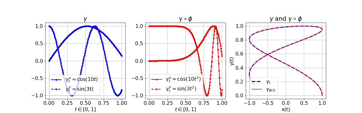
An important obstacle that most machine learning models have to face is the potential symmetry present in the data. In computer vision for example, a good model should be able to recognize an image even if the latter is rotated by a certain angle. The D rotation group, often denoted , is low dimensional (), therefore it is relatively easy to add components to a model that build a rotation invariance. However, when dealing with sequential data one is confronted with a much bigger (infinite dimensional) group of symmetries given by all reparametrizations of a path111Or its time-augmented version. (i.e. continuous and increasing surjections from the time domain of the path to itself). For example, consider the reparametrization given by and the path defined by where and . As it is clearly depicted in Fig. 1, both channels () of are individually affected by the reparametrization , but the shape of the curve is left unchanged.
Definition 1.1.
Let be a Banach space. The spaces of formal polynomials and formal power series over are defined respectively as
| (1) |
where denotes the (classical) tensor product of vector spaces. Both and can be endowed with the operations of addition and multiplication defined for any two elements and respectively as
| (2) | ||||
| (3) |
When endowed with these two operations and the natural action of by , becomes a real, non-commutative unital algebra with unit called the tensor algebra. The truncated tensor algebra over of order is defined as the quotient by the ideal
| (4) |
Definition 1.2.
Let be a compact interval, a Banach space and let be a continuous path of finite -variation (Definition B.4) with . For any such that , the signature of the path over the sub-interval is defined as the following infinite collection of iterated integrals
| (5) |
The signature (Definition 1.2) of a path is invariant under reparametrization (i.e. ), therefore it acts on as a filter that systematically removes this troublesome, infinite dimensional group of symmetries. Furthermore, it turns out that linear functionals acting on the range of the signature form an algebra (with pointwise multiplication) and separate points [2, chapter 2]. Hence, by the Stone-Weierstrass theorem, for any compact set of continuous paths of bounded variation, the set of linear functionals on signatures of paths from is dense in the set of continuous real-valued functions on . These two properties make the signature an ideal feature map for data streams [3].
For any path of finite -variation () the terms in the signature decay factorially according to the following uniform estimate [3, Lemma 5.1]
| (6) |
where denotes any norm on and denotes the -variation of the path restricted to the interval . Therefore, the collection of iterated integrals in the signature is graded. This grading allows one to truncate the signature at a finite level and consider only a finite collection of integrals as features extracted from
| (7) |
However, it is clear that the (truncated) signature has an exponential growth in the number of features, limiting its successful direct usage to machine learning applications where the ambient space of the data streams is relatively low dimensional [4, 5, 6, 7, 8, 9, 10].
Kernel methods [11] have shown to be efficient learning techniques in situations where inputs are non-euclidean, high-dimensional (not necessarily sequential) and the number of training instances is limited [12] so that deep learning methods cannot be easily deployed. Most kernels that are used in practice can be computed efficiently without referring back to the corresponding feature map, a mechanism known as kernel trick. When the data is sequential, the design of appropriate kernel functions is a notably challenging task [13]. In [1] the authors introduce the truncated signature kernel as the inner product of two truncated signatures and propose an efficient algorithm to compute this kernel starting from any “static” kernel on the ambient space of the input paths.
One of our goals will be to extend the results in [1] and consider the (untruncated) signature kernel as an inner product of two (untruncated) signatures. For this, leveraging a fundamental property of the signature (Theorem 2.3), we prove in Section 2 that if the two input paths are continuously differentiable then the signature kernel is the solution of a linear, second order, hyperbolic partial differential equation (PDE). In Section 3 we recognize the connection between the signature kernel PDE and a class of differential equations known in the literature as Goursat problems [14]. This PDE represents effectively a kernel trick for the signature kernel and can be efficiently solved numerically leveraging any state-of-the-art hyperbolic PDE solvers; we provide ourselves a competitive finite difference explicit scheme and demonstrate the improvement in computational performance over existing approximation methods. In Section 4 we extend the previous analysis to the much broader class of geometric rough paths, and show that in this case the signature kernel satisfies an integral equation analogous to the aforementioned Goursat PDE. Finally in Section 5, we empirically demonstrate the effectiveness of the signature kernel on various data science applications dealing with sequential data.
We release the python library sigkernel implementing our signature PDE kernel and various other functionalities deriving from it. All the experiments presented in this paper are reproducible following the instructions in https://github.com/crispitagorico/sigkernel.
Remark 1.3.
A concise summary of rough path theory, covering the material necessary to follow the proofs in Section 4, is presented in Appendix B. We note that an efficient algorithm for computing the truncated signature kernel was derived in [1] and then used in [15] in the context of Gaussian processes indexed on time series. Finally, we note that the article [16] first treated the truncated signature kernel in the case of branched rough paths. Integration of two parameters rough integrals is also discussed in [17].
2 The Signature Kernel is the solution of a hyperbolic PDE
In this section we present our main result, notably that the signature kernel evaluated at two continuously differentiable paths is the solution of a hyperbolic PDE. Throughout this section, we will denote by the space of continuously differentiable paths defined over an interval and with values on a Banach space . We will also use the lighter notation to denote the signature of a path over the interval , for any .
Definition 2.1.
Let be a -dimensional Banach space with canonical basis . It is easy to verify that for any the elements
| (8) |
form a basis of . Consider the inner product on defined on basis elements as
| (9) |
The inner product can be extended by linearity to an inner product on defined for any in as
| (10) |
Remark 2.2.
It is easy to verify that the space has the following algebraic property that we will refer to as coproduct property. Let be two positive integers and consider any two elements and any two basis elements seen as elements of , i.e. as and respectively. Then the following identity holds
| (11) |
As anticipated in the introduction, the signature has a fundamental characterisation in terms of controlled differential equations (CDEs) (see Section B.1 for a brief account on CDEs). In effect, the signature solves the universal differential equation stated in the next theorem, and therefore it can be equivalently defined as the non-commutative exponential.
Theorem 2.3.
[2, Lemma 2.10] Let be a continous path of finite -variation for and . Consider the vector field 222 denotes the space of bounded linear maps from to .
| (12) |
Then, the unique solution to the following controlled differential equation
| (13) |
is the signature of the path . Eq. 13 can be formally rewritten as
| (14) |
which explains why the signature of can be described as its non-commutative exponential.
2.1 The Signature Kernel PDE
Definition 2.4.
Let and be two compact intervals and let and . The signature kernel is defined as
| (15) |
The following is the main result of this section; it unveils a simple relation between the signature kernel and a class of hyperbolic PDEs.
Theorem 2.5.
Let and be two compact intervals and let and . The signature kernel is a solution of the following linear, second order, hyperbolic PDE
| (16) |
where , are the derivatives of and at time and respectively.
Proof 2.6.
Clearly, for any one has
and similarly for any . Recall that the signature of a path satisfies Eq. 14, which is equivalent to the following integral equation
where . Similarly for . Hence, we can compute
| (Theorem 2.3) | |||||
| (differentiability) | |||||
| (17) | (linearity) | ||||
| (coproduct property Eq. 11) | |||||
| (definition of ) | |||||
Note that the inner product and the double integral can be interchanged in Eq. 17 because of the factorial decay (Eq. 6) of the terms in the signature. By the fundamental theorem of calculus we can differentiate firstly with respect to
and then with respect to to obtain the PDE Eq. 16
Remark 2.7.
In Theorem 2.5 we have assumed the two input paths to be of class . However, one can lower this regularity assumption and consider two continuous paths of bounded variation and obtain the following integral equation
| (18) |
where is a quantity we are going to give meaning in Section 4, when we will consider the broader class of geometric rough paths. We note that one can make sense of the PDE Eq. 16 in Theorem 2.5 for piecewise paths.
Sequential information often arrives in the form of complex data streams taking their values in non-trivial ambient spaces. A good learning strategy would be to first lift the underlying ambient space to a (possibly infinite dimensional) feature space by means of a feature map on static data (RBF, Matern etc.), and then consider the signature kernel of the lifted paths as the final learning tool [1]. A question that naturally arises is whether one can compute the signature PDE kernel of the lifted paths from the static kernel associated to this feature map. [1] propose an algorithm to perform this procedure. Next, we provide an explanation of this procedure in the language of Banach spaces and PDEs.
2.2 The signature PDE kernel from static kernels on the ambient space
A kernel can be identified with a pair of embeddings of a set into a Banach space and its topological dual we denote this pair of maps by and A kernel induces a function through the natural pairing between a Banach space and its dual
| (19) |
Commonly, is assumed to be a Hilbert space, in which case can be taken to be the composition where is the canonical isomorphism coming from the Riesz representation theorem, yielding . It is unnecessary however for the general picture for to be a Hilbert space. In the general framework, a given pair of paths and , with , can be lifted to paths on and respectively as follows
| (20) |
If we assume that and are continuous and have bounded variation, then their signatures are well defined and belong to , which is again a Banach space with for any [2]. Hence, starting with a kernel on , the signature kernel is well-defined
| (21) |
If furthermore we assume that the lifted paths are of class Theorem 2.5 applies, yielding the following PDE
| (22) |
With a first order finite difference approximations for the derivatives , the PDE Eq. 22 can be entirely expressed in terms of the static kernel and underlying paths as follows
| (23) |
Remark 2.8.
We note that it is possible to establish our Goursat PDE Eq. 16 from the results [18, Proposition 4.7 p. 16], [18, Theorem 4., Appendix A], but this requires additional arguments as we shall explain next. Using their notation, given two differentiable paths , the truncated (at level ) signature kernel satisfies the following equation
where and where is a kernel on the ambient space of the paths. The first step towards a PDE is to realise that the first integrand in the last equation is itself the truncated signature kernel, truncated at level , yielding the expression
| (24) |
The untruncated signature kernel is obtained by taking the limit in Eq. 24 when . The factorial decay in the terms of the signature yields uniform convergence of this limiting process. Two uniformly convergent sequences of functions that are equal for all finite levels they are also equal in the limit, which implies
| (25) |
Finally one substitutes . At that point (and similarly to our argument in Theorem 2.5) one can differentiate both sides of Eq. 25 to get the Goursat PDE.
In the next section we recognize the link between Eq. 16 and a class of differential equation known in the literature as Goursat problems and propose a competitve numerical solver for our specific PDE.
3 A Goursat problem
Eq. 16 is an instance of a Goursat problem, which is a class of hyperbolic PDEs introduced in [14]. The PDE (16) is defined on the bounded domain
| (26) |
and its existence and uniqueness (for paths of class ) are guaranteed by setting the functions and in the following result.
Theorem 3.1.
[19, Theorems 2 & 4] Let and be two absolutely continuous functions whose first derivatives are square integrable and such that . Let be a bounded and measurable over and be square integrable. Then there exists a unique function such that and (almost everywhere on )
| (27) |
If in addition () and and are , then the unique solution of the Goursat problem is of class .
In the case of the signature PDE kernel, if the two input paths are of class , then their derivatives will be of class , and therefore Theorem 3.1 implies that the solution of the PDE Eq. 16 will be of class .
3.1 Finite difference approximation
In this section, we propose a numerical method based on an explicit finite difference scheme to approximate the solution of the Goursat PDE Eq. 16. To simplify the notation, we consider the case where . If and are piecewise linear, then the PDE Eq. 16 becomes
| (28) |
on each domain where is constant. In integral form, the PDE Eq. 28 can be written as
| (29) |
for with and . By approximating the double integral in Eq. 29, we can derive the following numerical explicit scheme
| (30) | ||||
Remark 3.2.
As one might expect, more sophisticated approximations can be derived by applying higher order quadrature methods to the double integral in (29) (see [20, 21] for specific examples).
Let be a partition of the interval and be a partition of the interval . Using the above, we can define finite difference schemes on the grid (and its dyadic refinements).
Definition 3.3.
For , we define the grid as the dyadic refinement of such that .
On the grid , we define the following explicit finite difference scheme for the PDE Eq. 16
| (32) | ||||
Remark 3.4.
If and are piecewise linear paths with respect to the coarsest grid then for some and .
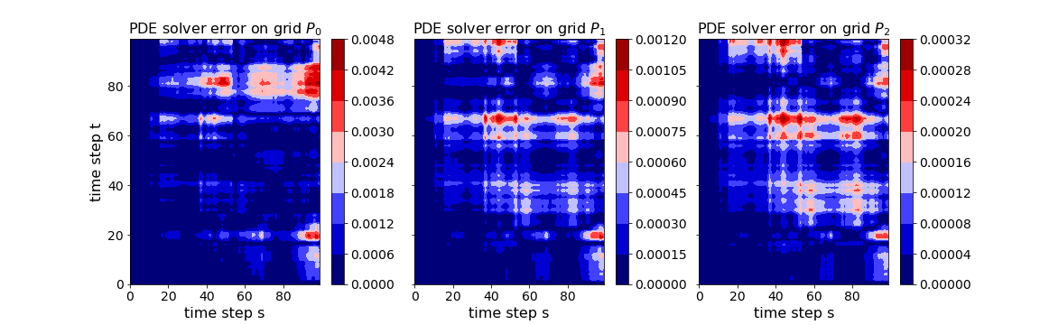
The explicit finite differences scheme Eq. 32 has a time complexity of on the grid , where is the dimension of the input streams and denote their respective lengths. Theorem 3.5 (which is the proved in Appendix A) ensures that by refining the discretization of the grid used to approximate the PDE, we get convergence to the true value. In practice we found that provided the input paths are rescaled so that their maximum value across all times and all dimensions is not too large (), coarse partitioning choices such as or are sufficient to obtain a highly accurate approximation, as shown in Fig. 2.
Theorem 3.5 (Global error estimate, Appendix A).
Let be a numerical solution obtained by applying one of the proposed finite difference schemes (Eq. 32) to the Goursat problem Eq. 16 on where and are piecewise linear with respect to the grids and . In particular, we are assuming there exists a constant , that is independent of , such that
| (33) |
Then there exists a constant depending on and , but independent of , such that
| (34) |
3.1.1 GPU implementation of the Goursat PDE
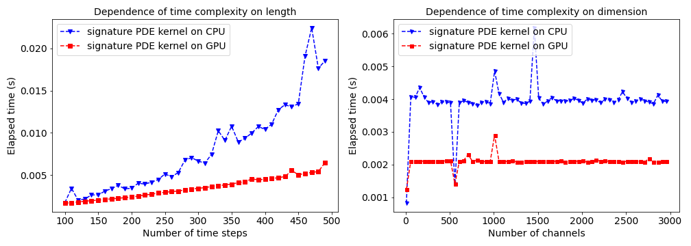
As mentioned earlier, the time complexity for one signature PDE kernel evaluation is on , where is the number of channels of the input time series and is their (maximum) length. Therefore, the complexity is quadratic in the length of the time series, which makes kernel evaluations computationally expensive for long time series. This also holds for the algorithm proposed in [1]. However, it is possible to parallelize the PDE solver by observing that instead of solving the PDE in row or column order, we can update the antidiagonals of the solution grid: each cell on an antidiagonal can be updated in parallel as there is no data dependency between them. This breaks the quadratic complexity, that becomes linear in the length , provided the number of threads in the GPU exceeds the size of the discretization. as shown in Fig. 3. This parallelization is possible thanks to the “PDE structure” of the problem, representing a considerable computational gain of our algorithm compared to the one proposed by [1]. We also note that the linear dependency on the number of channels of the input time series allows for the evaluation of the signature PDE kernel on time series with thousands of channels. Our library sigkernel offers the ability to evaluate kernels on a CPU using an optimized cython implementation as well as on CUDA if GPUs are available to the user.
In Section 5 we will present various applications of the signature kernel to time series classification and regression problems. But first we continue our theoretical analysis and drop the smoothness assumption on the input paths and extending the definition of signature kernel to far less regular classes of paths, namely geometric rough paths. The need to investigate the rough version of the signature kernel can be motivated also from several practical viewpoints. For example, this kernel can be used to derive an (unbiased) estimator for the maximum mean discrepancy (MMD) distance between distributions on path-space [16, sections 7, 8]. The MMD distance itself is useful to train models such as neural SDEs [22, 23, 24, 25], that is to fit neural SDEs to time series data. Since SDE solutions are geometric p-rough paths, Theorem 4.13 provides a candidate for the limiting kernel as the mesh size of the SDE discretization tends to zero. In particular, it guarantees that the signature kernel doesn’t “blow-up” in the limit. Another area where the rough signature kernel could be relevant is quantitative finance, where rough volatility models [26, 27] try to calibrate differential equation driven by fractional Brownian motion, which is a rough path if the Hurst exponent .
4 The signature kernel for geometric rough paths
Here we extend the notion of signature kernel developed in Section 2 to the broader class of geometric rough paths. To follow the material presented in this section we assume that the reader has some level of familiarity with basic concepts of rough path theory. We provide a brief summary of this theory in Appendix B. We begin by clarifying what we mean by signature of a geometric -rough path.
4.1 The signature of a geometric rough path
Definition 4.1.
The signature of a geometric -rough path (Definition B.17) controlled by a control (Definition B.11) is its unique extension to a multiplicative functional (Definition B.10) on as given by the Extension Theorem B.14.
From now on, we will denote by the space of geometric -rough paths over . Because all the sums in are finite, is an inner product space. Hence, denoting by the completion of , is a Hilbert space. Let be the norm on induced by the inner product , i.e. defined for any as , where is the norm on induced by , for any . In summary, we have the following chain of inclusions
| (35) |
Note that .
Lemma 4.2.
Let be a geometric -rough path defined over the simplex . Then, for any one has .
Proof 4.3.
To prove the statement of the lemma it suffices to find a sequence of tensors that convergences to in the -topology. Setting , and using the bounds from the Extension Theorem B.14 we have
| (36) |
which is clearly a convergent series because of the terms decay factorially, and
| (37) |
Next we present our second main result, that is we extend the definition of signature kernel to the space of geometric -rough paths (Definition B.17) and show that this rough version of the signature kernel solves an iterated double integral equation of two one-forms analogous to the Goursat PDE Eq. 16 presented in Section 2.
4.2 The signature kernel for geometric rough paths
In what follows will denote the following two simplices
| (38) | ||||
| (39) |
where are positive scalars such that and .
Definition 4.4.
Let be two scalars. Let and be two geometric - and -rough paths respectively and controlled by two controls and respectively. The (rough) signature kernel is defined for any and as follows
| (40) |
where the inner product is taken in .
Remark 4.5.
On the one hand, the signature kernel of Definition 2.4 is configured to act on two time indices and is indexed on two paths. This choice was made in order to differentiate with respect to these and obtain the PDE Eq. 16. On the other hand, the rough signature kernel of Definition 4.4 acts on two (rough) paths and is indexed on time indices. When dealing with highly oscillatory objects like rough paths studied in this section, one can’t expect to obtain a PDE, as these paths are far from being differentiable (even locally). However, we will nonetheless be able to use a density argument to prove our main result (Theorem 4.13).
Next we show that the rough signature kernel is bounded and continuous.
Lemma 4.6.
For any and any
| (41) |
Furthermore, the rough signature kernel is continuous with respect to the the product -variation topology.
Proof 4.7.
For any and by definition of the inner product on we immediately have
Consider now the function defined as follows
| (42) |
and the function defined as follows
| (43) |
The map is clearly continuous in both variables in the sense of . By the Extension Theorem B.14 we know that the two maps that extend (uniquely) and respectively to multiplicative functionals on the full tensor algebra are continuous in the - and -variation topologies respectively. Therefore is also continuous in both of its variables. Hence, is also continuous in both variables as it is the composition of two continuous functions.
In the next section we present our second main result. The core technical tool we use in the proof is the notion of integral of a one-form along a rough path, discussed in Section B.6.
4.3 A rough integral equation
To prove our main result we ought to give a meaning to the following double integral
| (44) |
We do so by constructing a double rough integral constructed as the composition of two one-forms (Definition B.6) as we shall explain next. In what follows we let .
Remark 4.8.
In the following construction, the spaces are swapped compared to the notation used in Section B.6.
For a fixed tensor , consider the linear one-form defined as follows333Perhaps more explicitly: for any , .: for any
| (45) |
where is the identity on and where the inner product is taken in .
Remark 4.9.
Note that a linear one-form is for all (Definition B.6). Hence, by Definition B.22 of integral of a one-form along a rough path, we can integrate along any geometric -rough path with .
For any and for any fixed geometric -rough path , consider now a second linear one-form defined as follows: for any and for any
| (46) |
where the inner product is taken in .
Remark 4.10.
Note that the rough integral is a -rough path with values in (and that, by the Extension Theorem B.14, its values in are also uniquely determined). Here, with the notation we mean the canonical projection of the rough path onto .
Remark 4.11.
We note that for any , the data in is ignored by both one-forms and when acting on . We preferred to keep this notation as we find it more in line with the standard notation used in rough integration.
As the one-form is for all , we can integrate along any -rough path with and use this integral as definition for the double integral of Eq. 44.
Definition 4.12.
Let the two simplices and be two scalars. Let and be two geometric - and -rough paths respectively. For any and any , define the double rough integral as
| (47) |
Note that this definition doesn’t depend on the order of integration of and . Next is our second main result, an analogue of Theorem 2.5 for the case of geometric rough paths.
Theorem 4.13.
Let the two simplices, be two scalars, and let and be two geometric - and -rough paths respectively. For any and any the rough signature kernel of Definition 4.4 satisfies the following equation
| (48) |
where is the double rough integral of Definition 4.12.
Proof 4.14.
By [2, Theorem 4.12] if is a geometric -rough path and is a one-form for some , then the mapping is continuous from to in the -variation topology.
For any and any both and defined in Equations Eq. 45 and Eq. 46 respectively are linear one-forms, hence for any . Similarly if . Thus, for any and any , the map is continuous in the -variation product topology.
By Lemma 4.6, the rough signature kernel is also continuous with respect to the -variation product topology.
Following the exact same steps as in the proof of Theorem 2.5, if and are both of bounded variation then the following double integral equation holds
| (49) |
which is equivalent to the equality .
By Definition B.17 of a geometric - (respectively -) rough path as the limit of -rough paths in the - (respectively -) variation topology, the space of continuous paths of bounded variation is dense (respectively ). Two continuous functions that are equal on a dense subset of a set are also equal on the whole set. The functional equation holds on , which concludes the proof by the previous density argument.
This is the last theoretical result of this paper. In Section 5 we tackle various machine learning tasks dealing with time series data.
5 Data science applications
In this section we evaluate our signature PDE kernel on three different tasks. Firstly, we consider the task of multivariate time series classification on UEA444Data available at https://timeseriesclassification.com datasets [28] with a support vector classifier (SVC) and compare the performance obtained by equipping the same SVC configuration with various kernel functions, including ours. Secondly, we run a regression task to predict future (average) bitcoin prices from previously observed prices by means of a support vector regressor (SVR) and similarly to the previous experiment, we compare the performance produced by a variety of kernels. Lastly, we show how the signature kernel can be easily incorporated within simple optimization procedure to represent the distribution of a large ensemble of paths as a weighted average of a small number of selected paths from the ensemble whilst maintaining certain statistical properties [29].
In presence of sequential inputs, well-designed kernels must be chosen with care. [30]. In the case where all the time series inputs are of the same length, standard kernels on can be deployed by stacking each dimension of the time series into one single vector. Standard choices of kernels include the linear and Gaussian (a.k.a. RBF) kernels. When the series are not of the same length, other kernels specifically designed for time series can be used to address this issue. Other than the signature PDE kernel introduced in this paper, to our knowledge only two other kernels for sequential data have been proposed in the literature: the truncated signature kernel [1] (Sig() - where denotes the truncation level) and the global alignment kernel (GAK) [13]. For the classification and regression experiments we made use of the SVC and SVR estimators respectively, from the popular python library tslearn [31].
Hyperparameter selection
The hyperparameters of the SVC and SVR estimators were selected by cross-validation via a grid search on the training set. For the classification we used the train-test split as provided by UEA, whilst for the regression we used a 80-20 split. Both the SVC and SVR estimators depend on a kernel and on two scalar parameters and . The range of values for was chosen to be and the one for to be for all kernel functions included in the comparison. We benchmark our Sig-PDE kernel against the Linear, RBF and GAK [13] kernels as well as the truncated signature kernel Sig() from [1]. We found that the algorithm provided to us by [32] was in general slower than directly computing the truncated signatures with iisignature [33]. This is because the former was implemented as pure python code, whilst iisignature is highly optimized and uses a C++ backend. For this reason, we ended up computing Sig() without kernel trick for all the experiments. The truncation is chosen from the range . Furthermore, we added a variety of additional hyperparameters to Sig() consisting in: 1) scaling the paths by different scalar scales, 2) normalizing the truncated signatures by multiplying (or not) each level by , 3) equipping the SVC/SVR with a Linear or RBF kernel (indexed on truncated signatures). For our Sig-PDE we used the RBF-lifted version with parameter taken in the range . All the experiments are reproducible using the code in https://github.com/crispitagorico/sigkernel and following the instructions thereafter.
5.1 Multivariate time series classification
The support vector classifier (SVC) [34] is one of the simplest yet widely used supervised learning model for classification. It has been successfully used in the fields of text classification [35], image retrieval [36], mathematical finance [37], medicine [38] etc. We considered various UEA datasets [28] of input-output pairs where each is a multivariate time series and each is the corresponding class. In Table 1 we display the performance of the same SVC equipped with different kernels (including ours). As the results show, our Sig-PDE kernel is systematically among the top classifiers across all the datasets (except for FingerMovements and UWaveGestureLibrary) and always outperforms its truncated counterpart, that often overfits during training.
| Datasets/Kernels | Linear | RBF | GAK | Sig(n) | Sig-PDE |
|---|---|---|---|---|---|
| ArticularyWordRecognition | 98.0 | 98.0 | 98.0 | 92.3 | 98.3 |
| BasicMotions | 87.5 | 97.5 | 97.5 | 97.5 | 100.0 |
| Cricket | 91.7 | 91.7 | 97.2 | 86.1 | 97.2 |
| ERing | 92.2 | 92.2 | 93.7 | 84.1 | 93.3 |
| Libras | 73.9 | 77.2 | 79.0 | 81.7 | 81.7 |
| NATOPS | 90.0 | 92.2 | 90.6 | 88.3 | 93.3 |
| RacketSports | 76.9 | 78.3 | 84.2 | 80.2 | 84.9 |
| FingerMovements | 57.0 | 60.0 | 61.0 | 51.0 | 58.0 |
| Heartbeat | 70.2 | 73.2 | 70.2 | 72.2 | 73.6 |
| SelfRegulationSCP1 | 86.7 | 87.3 | 92.4 | 75.4 | 88.7 |
| UWaveGestureLibrary | 80.0 | 87.5 | 87.5 | 83.4 | 87.0 |
5.2 Predicting Bitcoin prices
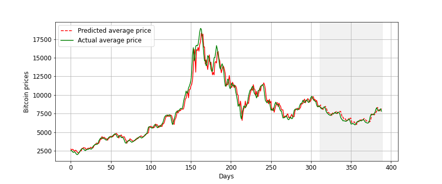
In the last few years, there has a remarkable rise of cryptocurrency trading where the most popular currency, Bitcoin, reached its peak at almost USD/BTC at the end of the year 2017 followed by a big crash in November 2018, when the price dropped to around USD/BTC. In this section, we will use daily Bitcoin to USD prices data555Data is from https://www.cryptodatadownload.com/ from Gemini which is one of the biggest cryptocurrency trading platforms in the US. Our goal is to use a window of size days to predict the mean price of the next days. As shown in Table 2, SVR equipped with the Sig-PDE is able to generalise better to unseen prices and produces better predictions on the test set in terms of MAPE compared to all other benchmarks. We also note that the truncated signature kernel doesn’t seem to generalize well to unseen observation for this regression exmaple. In Fig. 4 we plot the predictions obtained with SVR-Sig-PDE on the train and test sets.
| Kernel | RBF | GAK | Sig(n) | Sig-PDE |
|---|---|---|---|---|
| MAPE | 4.094 | 4.458 | 13.420 | 3.253 |
5.3 Moments-matching reduction algorithm for the support of a discrete measure on paths
As described in [39], herding refers to any procedure to approximate integrals of functions in a reproducing kernel Hilbert space (RKHS). In particular, such procedure can be useful to estimate kernel mean embeddings (KMEs) as we shall explain next. Consider a set and a feature map from to an RKHS with being the associated positive definite kernel. All elements of may be identified with real functions on defined by for . Following [40] for a fixed probability measure on we seek to approximate the KME , that belongs to the convex hull of [41]. To approximate , we consider points combined linearly with positive weights that sum to . We then consider the discrete measure and as shown in [41] we have that
| (50) |
which means that controlling is enough to control the error in computing the expectation for all with norm bounded by . We are interested in the setting where is a set of paths of bounded variation taking values on a -dimensional space (or in practice a set of multivariate time series for example). The signature being a natural feature map for sequential data we set , to be the untruncated signature kernel and . Following [42, 29], we consider the problem of reducing the size of the support in of a discrete measure whilst preserving some of its statistical properties. Suppose , where is large, and . We call a measure on a reduced measure with respect to if
We fix the size of the support of the reduced measure to be , so that . Because of condition 1) we have that is of the form , where all but of the weights ’s are equal to . Therefore the vector of weights is sparse. We are interested in the following optimization problem
where is the signature kernel. This minimisation will not yield a sparse vector . To induce sparsity we use an penalisation on the weights as in LASSO, which amounts to the following Lagrangian minimisation
| (51) |
where is a penalty parameter determined by the size of the support of . Equation (51) minimises a function that can be decomposed as , where is differentiable and is convex but non-differentiable, so a gradient descent algorithm can’t be directly applied. Subgradient descent methods are classical algorithms that address this issue but have poor convergence rates [43]. A better choice of algorithms for this particular problem are called proximal gradient methods [44]. Define the soft-thresholding operator as follows
| (52) |
Then, it can be shown [44] that is a minimiser of the optimisation (51) if and only if solves the following fixed point problem
| (53) |
The fixed point problem Eq. 53 can be solved iteratively fixing and for
| (54) |
Proximal gradient descent methods convergence with rate which is an order of magnitude better that the convergence rate of subgradient methods [44].
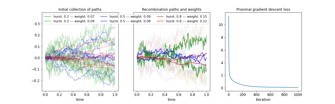
We apply the above proximal gradient descent algorithm to an example of a set of sample paths of fractional Brownian Motion (fBM) with Hurst exponent drawn uniformly at random from (note that fBM() corresponds to Brownian motion). The goal is to compute a reduced measure with smaller support size. We choose a value of the penalisation constant in Eq. 51 so that the new support is of size . The selected paths with corresponding weights are displayed in Fig. 5. This selection is clearly well-balanced across the samples ( paths per exponent) so more likely to well-represent the initial ensemble.
6 Conclusion
In this paper we introduce the signature PDE kernel and show that when paths are continuously differentiable the latter solves a hyperbolic PDE. We recognize the connection with a well known class of differential equations known in the literature as Goursat problems. Our Goursat PDE can be solved numerically using state-of-the-art hyperbolic PDE solvers; we propose an efficient finite different scheme to do so that has linear time complexity when implemented on GPU and analyse its convergence properties. We extend the previous analysis to the case of geometric rough paths and establish a rough integral equation analogous to the aforementioned Goursat problem. Finally we demonstrated the effectiveness of our kernel in various data science applications dealing sequential data.
Acknowledgements
We thank Maud Lemercier for her help with the implementation of sigkernel, Franz Kiraly and Harald Oberhauser for the helpful comments and the referees for pointing out an error in the experiments in the previous version of the paper.
References
- [1] Franz J Király and Harald Oberhauser. Kernels for sequentially ordered data. Journal of Machine Learning Research, 2019.
- [2] Terry Lyons, Michael Caruana, and Thierry Lévy. Differential equations driven by rough paths. Ecole d’été de Probabilités de Saint-Flour XXXIV, pages 1–93, 2004.
- [3] Terry Lyons. Rough paths, signatures and the modelling of functions on streams. International Congress of Mathematicians, Seoul, 2014.
- [4] Imanol Perez Arribas, Guy M Goodwin, John R Geddes, Terry Lyons, and Kate EA Saunders. A signature-based machine learning model for distinguishing bipolar disorder and borderline personality disorder. Translational psychiatry, 8(1):1–7, 2018.
- [5] James H Morrill, Andrey Kormilitzin, Alejo J Nevado-Holgado, Sumanth Swaminathan, Samuel D Howison, and Terry J Lyons. Utilization of the signature method to identify the early onset of sepsis from multivariate physiological time series in critical care monitoring. Critical Care Medicine, 48(10):e976–e981, 2020.
- [6] Patrick Kidger, Patric Bonnier, Imanol Perez Arribas, Cristopher Salvi, and Terry Lyons. Deep signature transforms. In Advances in Neural Information Processing Systems, volume 32, 2019.
- [7] Weixin Yang, Terry Lyons, Hao Ni, Cordelia Schmid, and Lianwen Jin. Developing the path signature methodology and its application to landmark-based human action recognition. arXiv preprint arXiv:1707.03993, 2017.
- [8] PJ Moore, TJ Lyons, J Gallacher, and Alzheimer’s Disease Neuroimaging Initiative. Using path signatures to predict a diagnosis of alzheimer’s disease. PloS one, 14(9):e0222212, 2019.
- [9] Thomas Cochrane, Peter Foster, Varun Chhabra, Maud Lemercier, Cristopher Salvi, and Terry Lyons. Sk-tree: a systematic malware detection algorithm on streaming trees via the signature kernel. arXiv preprint arXiv:2102.07904, 2021.
- [10] Terry Lyons, Sina Nejad, and Imanol Perez Arribas. Numerical method for model-free pricing of exotic derivatives in discrete time using rough path signatures. Applied Mathematical Finance, 26(6):583–597, 2019.
- [11] Thomas Hofmann, Bernhard Schölkopf, and Alexander J Smola. Kernel methods in machine learning. The annals of statistics, pages 1171–1220, 2008.
- [12] John Shawe-Taylor, Nello Cristianini, et al. Kernel methods for pattern analysis. Cambridge university press, 2004.
- [13] Marco Cuturi. Fast global alignment kernels. In Proceedings of the 28th international conference on machine learning (ICML-11), pages 929–936, 2011.
- [14] Edouard Goursat. A Course in Mathematical Analysis: pt. 2. Differential equations.[c1917, volume 2. Dover Publications, 1916.
- [15] Csaba Toth and Harald Oberhauser. Bayesian learning from sequential data using gaussian processes with signature covariances. In Proceedings of the international conference on machine learning (ICML), 2020.
- [16] Ilya Chevyrev and Harald Oberhauser. Signature moments to characterize laws of stochastic processes. arXiv preprint arXiv:1810.10971, 2018.
- [17] Khalil Chouk and Massimiliano Gubinelli. Rough sheets. arXiv preprint arXiv:1406.7748, 2014.
- [18] Franz J Király and Harald Oberhauser. Kernels for sequentially ordered data. arXiv preprint arXiv:1601.08169, 2016.
- [19] Milton Lees. The goursat problem. Journal of the Society for Industrial and Applied Mathematics, 8(3):518–530, 1960.
- [20] J. T. Day. A runge-kutta method for the numerical solution of the goursat problem in hyperbolic partial differential equations. The Computer Journal, 9:81–83, 1966.
- [21] A. M. Wazwaz. On the numerical solution for the goursat problem. Applied Mathematics and Computation, 59:89–95, 1993.
- [22] Belinda Tzen and Maxim Raginsky. Neural stochastic differential equations: Deep latent gaussian models in the diffusion limit. arXiv preprint arXiv:1905.09883, 2019.
- [23] Patrick Kidger, James Foster, Xuechen Li, Harald Oberhauser, and Terry Lyons. Neural sdes as infinite-dimensional gans. arXiv preprint arXiv:2102.03657, 2021.
- [24] Xuechen Li, Ting-Kam Leonard Wong, Ricky TQ Chen, and David K Duvenaud. Scalable gradients and variational inference for stochastic differential equations. In Symposium on Advances in Approximate Bayesian Inference, pages 1–28. PMLR, 2020.
- [25] Christa Cuchiero, Wahid Khosrawi, and Josef Teichmann. A generative adversarial network approach to calibration of local stochastic volatility models. Risks, 8(4):101, 2020.
- [26] Jim Gatheral, Thibault Jaisson, and Mathieu Rosenbaum. Volatility is rough. Quantitative Finance, 18(6):933–949, 2018.
- [27] Christian Bayer, Peter Friz, and Jim Gatheral. Pricing under rough volatility. Quantitative Finance, 16(6):887–904, 2016.
- [28] A. Bagnall, J. Lines, A. Bostrom, J. Large, and E. Keogh. The great time series classification bake off: a review and experimental evaluation of recent algorithmic advances. Data Mining and Knowledge Discovery, 31:606–660, 2017.
- [29] Francesco Cosentino, Harald Oberhauser, and Alessandro Abate. A randomized algorithm to reduce the support of discrete measures. arXiv preprint arXiv:2006.01757, 2020.
- [30] Nicholas I Sapankevych and Ravi Sankar. Time series prediction using support vector machines: a survey. IEEE Computational Intelligence Magazine, 4(2):24–38, 2009.
- [31] Romain Tavenard, Johann Faouzi, Gilles Vandewiele, Felix Divo, Guillaume Androz, Chester Holtz, Marie Payne, Roman Yurchak, Marc Rußwurm, Kushal Kolar, and Eli Woods. Tslearn, a machine learning toolkit for time series data. Journal of Machine Learning Research, 21(118):1–6, 2020.
- [32] C. Toth C. Salvi. personal communication.
- [33] Jeremy Reizenstein and Benjamin Graham. The iisignature library: efficient calculation of iterated-integral signatures and log signatures. arXiv preprint arXiv:1802.08252, 2018.
- [34] Vladimir Vapnik. The support vector method of function estimation. In Nonlinear Modeling, pages 55–85. Springer, 1998.
- [35] Simon Tong and Daphne Koller. Support vector machine active learning with applications to text classification. Journal of machine learning research, 2(Nov):45–66, 2001.
- [36] Simon Tong and Edward Chang. Support vector machine active learning for image retrieval. In Proceedings of the ninth ACM international conference on Multimedia, pages 107–118, 2001.
- [37] Wei Huang, Yoshiteru Nakamori, and Shou-Yang Wang. Forecasting stock market movement direction with support vector machine. Computers & operations research, 32(10):2513–2522, 2005.
- [38] Terrence S Furey, Nello Cristianini, Nigel Duffy, David W Bednarski, Michel Schummer, and David Haussler. Support vector machine classification and validation of cancer tissue samples using microarray expression data. Bioinformatics, 16(10):906–914, 2000.
- [39] Yutian Chen, Max Welling, and Alex Smola. Super-samples from kernel herding. In Proceedings of the Twenty-Sixth Conference on Uncertainty in Artificial Intelligence, pages 109–116, 2010.
- [40] Alex Smola, Arthur Gretton, Le Song, and Bernhard Schölkopf. A hilbert space embedding for distributions. In International Conference on Algorithmic Learning Theory, pages 13–31. Springer, 2007.
- [41] Francis R Bach, Simon Lacoste-Julien, and Guillaume Obozinski. On the equivalence between herding and conditional gradient algorithms. In ICML, 2012.
- [42] Christian Litterer, Terry Lyons, et al. High order recombination and an application to cubature on wiener space. The Annals of Applied Probability, 22(4):1301–1327, 2012.
- [43] Francis Bach, Rodolphe Jenatton, Julien Mairal, and Guillaume Obozinski. Optimization with sparsity-inducing penalties. Found. Trends Mach. Learn., 2012.
- [44] Mark Schmidt, Nicolas L Roux, and Francis R Bach. Convergence rates of inexact proximal-gradient methods for convex optimization. In Advances in neural information processing systems, pages 1458–1466, 2011.
- [45] Maud Lemercier, Cristopher Salvi, Theodoros Damoulas, Edwin V Bonilla, and Terry Lyons. Distribution regression for continuous-time processes via the expected signature. arXiv preprint arXiv:2006.05805, 2020.
- [46] Andrei D. Polyanin and Vladimir E. Nazaikinskii. Handbook of Linear Partial Differential Equations for Engineers and Scientists. 2nd Edition, Chapman and Hall/CRC, 2015.
- [47] George E. Andrews, Richard Askey, and Ranjan Roy. Special functions. Encyclopedia of Mathematics and its Applications, 71, 2001.
- [48] Terry J Lyons. Differential equations driven by rough signals. Revista Matemática Iberoamericana, 14(2):215–310, 1998.
- [49] Terry Lyons et al. Coropa computational rough paths (software library). 2010.
- [50] Patrick Kidger and Terry Lyons. Signatory: differentiable computations of the signature and logsignature transforms, on both CPU and GPU. arXiv:2001.00706, 2020.
- [51] Terry Lyons and Nicolas Victoir. An extension theorem to rough paths. In Annales de l’IHP Analyse non linéaire, volume 24, pages 835–847, 2007.
Appendix A Error analysis for the numerical scheme
In this section, we show that the finite difference scheme Eq. 32 achieves a second order convergence rate for the Goursat problem Eq. 16. Our analysis is based on an explicit representation of the PDE solution.
Theorem A.1 (Example 17.4 from [46]).
Consider the following specific case of the general Goursat problem (27) on the domain :
| (55) |
where is constant and the boundary data , is differentiable. Then the solution can be expressed as
| (56) |
for , where the Riemann function is defined as for , with denoting the zero order Bessel function of the first kind.
Remark A.2.
Using Theorem A.1 and the above identities, we will perform a local error analysis for the explicit scheme Eq. 32.
Theorem A.3 (Local error estimates for the explicit scheme).
Consider the Goursat problem Eq. 55 on the domain :
where is constant and the boundary data , is differentiable and of bounded variation. We define the local approximation error of the explicit scheme Eq. 32 as
Then
| (60) | ||||
In addition, if are twice differentiable and their derivatives have bounded variation, then
| (61) | ||||
Remark A.4.
From Eq. 57, it is clear that , and .
Proof A.5.
To begin, we decompose the approximation error as where
Since , , and , it follows that
Hence by (56), we can write where the error terms and are given by
The integrand of can be estimated as
| (62) | |||
By applying the formulae Eq. 58 and Eq. 59 to the function , we can compute its derivatives,
| (63) | |||
| (64) |
Therefore, it now follows from Eq. 62 and Eq. 63 that
and we can obtain a similar estimate for (where would appear instead of ). From the estimates for and , we have
Estimating is straightforward as
Using the above estimates for and , we obtain Eq. 60 as required. For the remainder of this proof we will assume that , are twice differentiable and , have bounded variation. In this case, we can apply the fundamental theorem of calculus to the integrand of so that
Note that by the well-known error estimate for the Trapezium rule, we have
Recall that this derivative was given by Eq. 64. It now follows from the above and Eq. 62 that
Applying the same argument to leads to the second estimate Eq. 61 as required.
From the estimate Eq. 61 we see that the proposed finite difference scheme achieves a local error that is when the domain has a small height and width of (and provided the boundary data is smooth enough). Since discretizing a PDE on an grid involves steps, we expect the proposed scheme to have a second order of convergence.
Theorem A.6 (Global error estimate).
Let be a numerical solution obtained by applying the proposed finite difference scheme (Definition 3.3) to the Goursat PDE Eq. 16 on the grid where and are piecewise linear with respect to the grids and . In particular, we are assuming there exists a constant , that is independent of , such that
Then there exists a constant depending on and , but independent of , such that
| (65) |
for all .
Proof A.7.
Using the solution , we define another approximation on as
It follows from theorem 3.1 that the PDE solution and boundary data are smooth on each small rectangle in . So by (61) there exists , depending on and , such that
Taking the difference between and gives
Hence by the triangle inequality, we obtain a recurrence relation for the approximation errors,
Since each and is proportional to , the result for the explicit scheme follows by iteratively applying the above recurrence relation.
Appendix B Background on rough path theory
In this appendix we present a brief summary of rough path theory explain all the necessary meterial required to understand the results presented in Section 4, which should be self-contained. We begin by explaining what a controlled differential equation (CDE) is.
B.1 Controlled differential equations (CDEs)
In a simplified setting where everything is differentiable a CDE is a differential equation of the form
| (66) |
where is a given path, is an initial condition, and is the unknown solution. If did not depend on its first variable, equation Eq. 66 would be a first order time-homogeneous ODE, the function would be a vector field, and would be the integral curve of starting at . If instead we had , then Eq. 66 would describe a first order time-inhomogeneous ODE, with solution being an integral curve of a time-dependent vector field . In the CDE Eq. 66 the time-inhomogeneity depends on the trajectory of , which is said to control the problem.
A CDE provides a fairly generic way to describe how a signal interacts with a control system of the form Eq. 66 to produce a response . For example, a CDE can model the interaction of an electricity signal (current, voltage) with a domestic appliance (e.g. a washing machine) to produce a response (e.g. the rotation speed or the water temperature).
Throughout this appendix will be two Banach spaces and will denote the set of bounded linear maps from to . We will denote by a generic compact (time) interval. Consider two continous paths and and a continuous function , and let’s assume that and are regular enough for the integral to make sense for any 666In what follows we will discuss various regularity assumptions on ..
Given an initial condition , we say that and satisfy the following controlled differential equation (CDE)
| (67) |
if the following equality holds for all
| (68) |
Here is called a vector field, the control driving the equation and the response solution.
Remark B.1.
If is a solution of Eq. 67 driven by and if is an increasing surjection (also called time-reparametrization), then is also a solution to the same equation driven by . In other words, solutions of CDEs are invariant to time-reparametrization.
Remark B.2.
The definition of as a continuous function from to makes the notation in Eq. 67 clear. However, there is another equivalent interpretation of which is important to keep in mind. Let be the space of continuous functions from to . Then can be thought of as an element of . Adopting this point of view, is a linear function on with values in the space of vector fields on . To make this view compatible with Eq. 67 it is perhaps easier to think of the CDE Eq. 67 using a slightly different notation: . This alternative point of view has a deep physical interpretation: at each time the solution describes the state of a complex system that evolves as a function of its present state and of an infinitesimal external parameter controlling it. The function transforms the infinitesimal displacement into a vector field that defines a direction for the trajectory of to follow.
B.2 CDEs driven by paths of bounded variation
Definition B.3.
A continuous path is said to be of bounded variation if
| (69) |
where the supremum is taken over all partitions of an interval , i.e. over all increasing sequences of ordered (time) indices such that . We denote by the space of continuous paths of bounded variation with values in .
Definition B.4.
Let be a real number and be a continuous path. The -variation of on the interval is defined by
| (70) |
Remark B.5.
For any continuous path , any time-reparametrization and scalar one has ; in other words the -variation of is invariant to time-reparametrization. Furthermore, the function is decreasing. Hence, any path of finite -variation is also a path of finite -variation for any .
If one assumes that is of bounded variation and that and are continuous, then the integral exists for all (as a classical Riemann-Stieltjes integral). If is Lipschitz continuous then the solution is unique [2, Theorem 1.3 & 1.4].
B.3 CDEs driven by paths of finite -variation with
However, If our goal is to solve differential equations driven by more irregular paths we should be prepared to compensate by allowing more smoothness on the function . In particular, if and are real numbers such that and and has finite -variation, and if is Hölder continuous with exponent , then the CDE Eq. 67 admits a solution [2, Theorem 1.20]. In order to get uniqueness we require to be more regular than Hölder continuous. In the next definition we introduce a class of functions exhibiting the appropriate level of regularity to ensure uniqueness.
Definition B.6.
Let be Banach spaces, an integer, and a closed subset of . Let be a function. For each integer , let be a function taking its values in the space of symmetric -linear forms from to , where denotes the tensor product of vector space (that we will define more precisely in the next section). The collection is an element of if there exists a constant such that for each
| (71) |
and there exists a function such that for any and any
| (72) |
and
| (73) |
The smallest constant for which the inequalities above hold for all is called the -norm of and is denoted by . We will call such function a function (or one-form).
Remark B.7.
The best way to understand of a function is to think about it as a function that “locally looks like a polynomial function”. Let us explain the connection to paths. Let be an integer. Let be a polynomial of degree . Let be a continuous path of bounded variation. If denotes the derivative of then by Taylor’s theorem we have that for any
| (74) |
Substituting the expression of into in the last expression we get
| (75) |
where is the second derivative of , and is the space of bilinear forms on . Iterating the substitutions, the procedure stops at level yielding the following expression
| (76) |
where for each , denotes the derivative of which takes its values in the space of symmetric -linear forms on . The symmetric part of the tensor is equal to . Hence
| (77) |
The general concept of function where for some mimics closely the behaviour defined by equation Eq. 77 up to an error which is Hölder continuous of exponent . Indeed, using the notation from Definition B.6, if takes its values in a closed subset of , for any , any and any we have the following relation
| (78) |
which is analogous to Eq. 76. This is the general form of a function that we will consider from now on.
If and are such that and , is a continuous path of finite -variation and be a function, then for any , the CDE Eq. 67 admits a unique solution. Furthermore, if denotes the unique solution, then the function , that maps -valued paths of finite -variation to -valued paths of finite -variation, is continuous in the norm [2, Theorem 1.28].
We are now able to give meaning to CDEs where the control is not necessarily of bounded variation. However, if the driving path has finite -variation but infinite -variation for every , we are still not able to give a meaning to the CDE Eq. 67. This is quite a hard restriction given that Brownian paths have finite -variation only for .
To be able to push this barrier even further we first need to introduce some algebraic spaces and construct one of the central objects in rough path theory, the signature of a path. We do so very briefly in the next section and then explain in Section B.4 the connection with (linear) CDEs.
Remark B.8.
The -variation function defines a control.
B.4 The role of the signature to solve linear CDEs
It turns out that the sequence of iterated integrals of a path (i.e. its signature) in Definition 1.2 appears naturally when one wants to solve linear CDEs. In what follows, we show how the iterated integrals of a path precisely encode all the information that is necessary to determine the response of a linear CDE driven by this path.
Let be two Banach spaces. Let be a bounded linear map. Here will play the role of (linear) vector field defined with the alternative but equivalent point of view expressed in Remark B.2. Let be a continuous path of bounded variation. Consider the following system of linear CDEs
| (79) | ||||
| (80) |
where in the first equation the expression is to be read as and in the second expression means . The solution to Eq. 80 is called the flow associated to the linear equation Eq. 79. From the flow and the initial condition one gets the solution in the usual way
| (81) |
The map that to the pair associates the solution is generally called the Itô-map. We will now run an iterative procedure analogous to the Picard’s iteration for ODEs in order to obtain a sequence of flows, i.e. paths with values in the space of linear vector fields on . Firstly, we start by setting the first element of the sequence equal to the identity on and then we integrate Eq. 80 to get
| (82) |
Doing it again we obtain the following expression for the next element in the sequence
| (83) |
Iterating this process we get the following expression for the term in the sequence
| (84) |
Now, for any the linear operator can be extended to the operator as follows
| (85) |
which allows us to rewrite equation Eq. 84 as
| (86) |
where we can finally recognise the various terms of the signature of the path (see Definition 1.2) and how the latter fundamentally encode the information to solve linear CDEs. The sequence of approximations for the flow provides a sequence of approximations for the solution of the CDE Eq. 79:
| (87) |
It turns out that the speed at which the sequence of approximations converges to the true solution of the CDE Eq. 79 is extremely high.
Lemma B.9.
[2, Proposition 2.2] For each we have
| (88) |
In particular, taking any norm on bounded linear operators, the error decays factorially
| (89) |
This shows how the signature of a control provides an extremely efficient sequence of statistics to solve any linear CDE driven by (provided the norm of is not too large).
B.5 Multiplicative functionals and the Extension Theorem
In this section we push the limit on the regularity of the driver even further and explain how to solve CDEs driven by rough paths, as presented in the seminal paper [48]. This will demand to define what a (geometric) rough path is and to present a powerful theory of integration of one-forms along rough paths to what will follow the Universal Limit Theorem for CDEs driven by rough paths (Theorem B.26). In what follows, will denote the simplex
| (90) |
Definition B.10.
Let be an integer and let be a continuous map
| (91) |
is said to be a multiplicative functional if for all and
| (92) |
The Chen’s identity condition of Definition B.10 imposed to a multiplicative functional is a purely algebraic one. We are now going to describe an analytic condition for a multiplicative functional through the notion of -variation.
Definition B.11.
A control is a continuous non-negative function which is super-additive in the sense that
| (93) |
and for which for all .
Definition B.12.
Let be a real number and be an integer. Let be a control and be a multiplicative functional. We say that has finite -variation on controlled by if
| (94) |
where and where is a real constant that depends only on and that we will make explicit later in the chapter. We say that has finite -variation if there exists a control such that this condition is satisfied.
Definition B.13.
Let be two multiplicative functionals. The -variation metric is defined as follows
| (95) |
where denotes any norm on the corresponding level .
The next theorem is one of the fundamental results in rough path theory. It states that every multiplicative functional of degree and of finite -variation can be extended in a unique way to a multiplicative functional of arbitrarily high degree provided is greater than the integer part of , denoted by . Furthermore the extension map is continuous in the -variation metric.
Theorem B.14.
[2, Extension Theorems 3.7 & 3.10] Let be a real number and an integer. Let be a multiplicative functional of finite -variation controlled by a control . Assume that . Then, for any , there exist a unique continuous function such that
| (96) |
is a multiplicative functional of finite -variation controlled by according to the inequality Eq. 94 with
| (97) |
Moreover, the extension map is continuous in the -variation metric in the sense that if for some we have
| (98) |
then, provided
| (99) |
the bound Eq. 98 holds for all .
Definition B.15.
Let be a Banach space and be a real number. A -rough path in is a multiplicative functional of degree with finite -variation. We denote the space of -rough paths over by .
Hence, a -rough path is a continuous map from that satisfies an algebraic condition (Chen’s identity) and an analytic condition (finite -variation). As a consequence of the Extension Theorem (B.14), we get that every -rough path in has a full signature, i.e. it can be extended to a multiplicative functional of arbitrary high degree with finite -variation in .
Remark B.16.
Recall that a path of finite -variation has finite -variation for any . In particular, a path of bounded variation is a -rough path for any . We now dispose of all the necessary ingredients to define what a geometric -rough path is.
Definition B.17.
A geometric -rough path is a -rough path that can be expressed as the limit of a sequence of -rough paths in the -variation metric. We denote by the space of geometric -rough paths in .
Hence, is the closure in of the space of continuous paths of bounded variation. Next we apply the ideas developed so far in order to define a powerful theory of integration for solving differential equations driven by (geometric) rough paths.
B.6 Integration of a one-form along a rough path
In order to define what we mean by a solution of a differential equation driven by a rough path, we need a theory of integration for rough paths. The correct notion of integral turns out to be the integral of a one-form along a rough path. We start by defining the concept of almost -rough path.
Definition B.18.
Let be a real number. Let be a control. A function is called an almost -rough path if
-
1.
it has finite -variation controlled by , i.e.
(100) -
2.
it is an almost multiplicative functional, i.e. there exists such that
(101)
To be specific we say that is a -almost -rough path controlled by .
For any almost -rough path there exists a unique -rough path that it is close to it in some specific sense, as stated in the next theorem.
Theorem B.19.
[2, theorem 4.3 & 4.4] Consider two scalars and , a control . Let be a -almost -rough path controlled by . Then there exists a unique -rough path such that
| (102) |
Furthermore, the map that to an almost -rough path associates a rough path is continuous in -variation.
Remark B.20.
It is important to note that, if and are two -rough paths with , and is a map, even the smoothest one, it is not possible to give a sensible meaning to something like . In effect, as shown by the simple example , the definition of such object would necessarily involve some cross-iterated integrals of and , which are not available directly in the data of and . In other words, two rough paths and do not determine the joint path as a rough path in . However, if one knows the joint path as a rough path, then the integral can be defined as a special case of , where is a one-form. This is the object we are going to construct in the sequel.
We will define the integral of a one-form along a rough path as the unique -rough path associated to, in the sense of Theorem B.19, a specific almost -rough path that we now construct.
Let be scalars and let be a -rough path controlled by some control . Let be a function (Definition B.6) that we will call a one-form from now on. Hence, we are given and at least auxiliary functions such that for any
| (103) |
satisfying the Taylor-like expansion:
| (104) |
with , where is the Lipschitz constant of . We are going to look for an approximation of in the form of a Taylor expansion. For any we can write
| (105) |
Now, by definition of the iterated integrals of , the following relation holds for any
| (106) |
where with the multiplication we mean . Combining Eq. 105 and Eq. 106 we obtain
| (107) |
Let us now define the following -valued path
| (108) |
and let us compute the higher order iterated integrals of in such a way that it becomes an almost rough path. For any it can be shown after some tedious calculations that
| (109) |
It turns out that the we have just defined is an almost rough path, as stated in the next theorem. We will use this as our approximation for .
Theorem B.21.
We can now define the integral of the one-form along the rough path as the unique rough path associated to the almost rough path according to Theorem B.19.
Definition B.22.
Let and be as in Theorem B.21. The unique -rough path associated to by Theorem B.19 is called the integral of the one-form along the rough path and is denoted by .
Remark B.23.
As stated in [2, Theorem 4.12], the map is continuous in -variation from to .
Definition B.24.
Let be a continuous linear map between Banach spaces and be a geometric -rough path. The image of the rough path by the linear map is a rough path defined in the following way. induces a linear map from to which sends to . By linearity of the direct sum defining and , can be further extended to a linear map between these two spaces, denoted by . Then, is defined as the following rough path
| (110) |
In the next section we will finally describe how to solve CDEs driven by rough paths.
B.7 Non-linear CDEs driven by rough paths
In this section we explain how to solve CDEs driven by rough paths. As in the classical case of CDEs driven by paths of bounded variation, the existence and uniqueness of the solution depend on assumptions about the smoothness of the vector field.
Let be two Banach spaces and be two real numbers. Let be a one-form. Consider a geometric -rough path and a point . It is easy to see that when has finite -variation, the equation
| (111) |
is equivalent, up to translation of the initial condition , to the following system
| (112) | ||||
| (113) |
where for all . Consider now the one-form defined as follows
| (114) |
where is the identity map on . Then, when is of bounded variation, solving (114) is equivalent to finding such that
| (115) |
where is the canonical projection of onto . What the next definition states is that this reformulation makes sense even when is a rough path.
Definition B.25.
Consider the notation introduced above. We call a solution of the differential Eq. 111 if the following two conditions hold:
| (116) | |||
| (117) |
where is the image of the rough path by the linear map in the sense of Definition B.24.
In order to find a solution to the CDE Eq. 111 we are going to, once again, use Picard iteration. Define , where denotes the -rough path . Then, for any we define the sequence of rough paths
| (118) |
Let us now denote so that . One of the main results in the seminal paper [48] is the following Universal Limit Theorem (ULT). Note that for the solution to be unique we require one extra degree of smoothness on .
Theorem B.26 (Universal Limit Theorem (ULT)).
[2, Theorem 5.3] Let and be real numbers. Let be a function. For all and all the equation
| (119) |
admits a unique solution in the sense of Definition B.25. Furthermore, the rough path is the limit of of the sequence of rough paths defined above, and the mapping which sends to is continuous in -variation.
Appendix C Cross-integrals of the signature kernel
In this final section of the appendix, we provide another interpretation for the double integral of Eq. 44. We begin by recalling a generalization of the Extension Theorem B.14.
Definition C.1.
Let be an integer. We denote by the free nilpotent Lie group of step over .
Theorem C.2.
[51, Theorem 14] Let . Let be a closed normal subgroup of . If is a -valued continuous path of finite -variation, with , then there exists a continuous -valued geometric -rough path such that
where is the canonical homomorphism (projection) from to
.
Corollary C.3.
If , then a continuous -valued smooth path of finite -variation can be lifted to a geometric -rough path
Proof C.4.
It suffices to apply Theorem C.2 to , where and , with being the Lie bracket.
Without loss of generality let’s assume . is a geometric -rough path, therefore by the Extension Theorem can be lifted uniquely to a geometric -rough path . Let be any compact time interval such that such that there exists two continuous and increasing surjections and . Let and .
Consider the path defined as
| (120) |
is a continuous, -valued path of finite -variation. Firstly, we consider the product of algebras , where the product of elements is defined by the following operation: .
Now consider the free tensor algebra over the vector space . Let be the canonical inclusion of into and let be the linear map defined as .
Now let’s consider the map . By the universal property of there exists a unique algebra homomorphism such that .
But now has also the universal property, therefore there exists a unique algebra homomorphism such that , where is the canonical inclusion of into .
Note that is a group embedded in the product algebra and is a group embedded in the tensor algebra . Let be the map restricted to . Given that , this map is a surjective group-homomorphism. Therefore, by the First Group Isomorphism Theorem we have that , and
By Lemma C.2 there exists a continuous -valued geometric -rough path such that . Expanding out coordinate-wise we obtain
| (121) |
Note that all the cross-integrals of and do not contribute in the above expression, which nicely factors into two separate integrals: expression (121) tells us that the rough path does not depend on the lift used in the extension (from the joint path to the rough path ). The terms involved in the infinite sum on the right-hand-side of the equation (121) are all -projections of the signature of the signautre of the rough paths and .