Implications of the search for optical counterparts during the second part of the Advanced LIGO’s and Advanced Virgo’s third observing run: lessons learned for future follow-up observations

Abstract

Joint multi-messenger observations with gravitational waves and electromagnetic data offer new insights into the astrophysical studies of compact objects. The third Advanced LIGO and Advanced Virgo observing run began on April 1, 2019; during the eleven months of observation, there have been 14 compact binary systems candidates for which at least one component is potentially a neutron star. Although intensive follow-up campaigns involving tens of ground and space-based observatories searched for counterparts, no electromagnetic counterpart has been detected. Following on a previous study of the first six months of the campaign, we present in this paper the next five months of the campaign from October 2019 to March 2020. We highlight two neutron star - black hole candidates (S191205ah, S200105ae), two binary neutron star candidates (S191213g and S200213t) and a binary merger with a possible neutron star and a “MassGap” component, S200115j. Assuming that the gravitational-wave candidates are of astrophysical origin and their location was covered by optical telescopes, we derive possible constraints on the matter ejected during the events based on the non-detection of counterparts. We find that the follow-up observations during the second half of the third observing run did not meet the necessary sensitivity to constrain the source properties of the potential gravitational-wave candidate. Consequently, we suggest that different strategies have to be used to allow a better usage of the available telescope time. We examine different choices for follow-up surveys to optimize sky localization coverage vs. observational depth to understand the likelihood of counterpart detection.

1 Introduction

The observational campaigns of Advanced LIGO (Aasi et al, 2015) and Advanced Virgo (Acernese et al, 2015) revealed the existence of a diverse population of compact binary systems. Thanks to the continuous upgrades of the detectors from the first observing run (O1) over the second observing run (O2) up to the recent third observational campaign (O3), the gain in sensitivity leads to an increasing number of compact binary mergers candidates: 16 alerts of gravitational-wave (GW) candidates were sent to the astronomical community during O1 and O2, covering a total of 398 days (Abbott et al., 2019d), compared to 80 alerts for O3a and O3b, covering a total of 330 days. Some of the candidates found during the online searches were retracted after further analysis, e.g., only 10 out of the 16 alerts were confirmed as candidates during the O1 and O2 runs (Abbott et al., 2019d, a). Additional compact binary systems were found during the systematic offline analysis performed with re-calibrated data, e.g., Abbott et al. 2019a, resulting in 11 confirmed GW events. During O3a and O3b, 24 of 80 alerts have already been retracted due to data quality issues, e.g. LIGO Scientific Collaboration & Virgo Collaboration 2019m, 2020c.

GW detections improve our understanding of binary populations in the nearby Universe (distances less than $\sim$ 2 Gpc), and cover a large range of masses; these cover from $\sim$ 1–2.3 solar masses, e.g. Lattimer 2012; Özel & Freire 2016; Margalit & Metzger 2017; Rezzolla et al. 2018; Abbott et al. 2020b, for binary neutron stars (BNSs) to $\sim$ 100 solar masses for the most massive black hole remnants. They may also potentially constrain black hole spins (LIGO Scientific Collaboration & Virgo Collaboration, 2019a). For mergers including NSs, electromagnetic (EM) observations provide a complementary view, providing precise localizations of the event, required for redshift measurements which are important for cosmological constraints (Schutz, 1986); these observations may last for years at wavelengths outside the optical spectrum; for instance, X-ray photons were detected almost 1000 days post-merger in the case of GW170817 (Troja et al., 2020).

The success of joint GW and EM observations to explore the compact binaries systems has been demonstrated by the success of GW170817, AT2017gfo, and GRB170817A, e.g., Abbott B. P. 2017; Abbott et al. 2017b; Arcavi et al. 2017; Coulter et al. 2017; Lipunov et al. 2017; Mooley et al. 2017; Savchenko et al. 2017; Soares-Santos et al. 2017; Tanvir et al. 2013; Troja et al. 2017; Valenti et al. 2017. GRB170817A, a short $\gamma$-ray burst (sGRB) (Eichler et al., 1989; Paczynski, 1991; Narayan et al., 1992; Mochkovitch et al., 1993; Lee & Ramirez-Ruiz, 2007; Nakar, 2007), and AT2017gfo, the associated kilonova (Sari et al., 1998; Li & Paczynski, 1998; Metzger et al., 2010; Roberts et al., 2011; Kasen et al., 2017), were the EM counterparts of GW170817. Overall, this multi-messenger event has been of interest for many reasons: to place constraints on the supranuclear equation of state describing the NS interior (e.g. Abbott et al. 2019b; Radice et al. 2018; Radice & Dai 2019; Bauswein et al. 2017; Margalit & Metzger 2017; Rezzolla et al. 2018; Coughlin et al. 2018b; Coughlin et al. 2019b; Capano et al. 2020; Dietrich et al. 2020), to determine the expansion rate of the Universe (Abbott et al., 2017a; Hotokezaka et al., 2019; Coughlin et al., 2020; Dhawan et al., 2019; Dietrich et al., 2020), to provide tests for alternative theories of gravity (Ezquiaga & Zumalacárregui, 2017; Baker et al., 2017; Creminelli & Vernizzi, 2017; Abbott et al., 2019c), to set bounds on the speed of GWs (Abbott et al., 2017b), and to prove BNS mergers to be a production side for heavy elements, e.g., Pian et al. 2017; Watson et al. 2019a.

Numerical-relativity studies reveal that not all binary neutron star (BNS) and black hole- neutron star (BHNS) collisions will eject a sufficient amount of material to create bright EM signals, e.g., Bauswein et al. 2013; Hotokezaka et al. 2013; Dietrich & Ujevic 2017; Abbott et al. 2017c; Köppel et al. 2019; Agathos et al. 2019; Kawaguchi et al. 2016; Foucart et al. 2018; Krüger & Foucart 2020. For example, there will be no bright EM signal if a black hole (BH) forms directly after merger of an almost equal-mass BNS, since the amount of ejected material and the mass of the potential debris disk are expected to be very small. Whether a merger remnant undergoes a prompt collapse depends mostly on its total mass but also seems to be sub-dominantly affected by the mass-ratio (Kiuchi et al., 2019; Bernuzzi et al., 2020). EM bright signatures originating from BHNS systems depend on whether the NS gets tidally disrupted by the BH and thus ejects a large amount of material and forms a massive accretion disk. If the neutron star falls into the BH without disruption, EM signatures will not be produced. This outcome is mostly determined by the mass ratio of the binary, the spin of the black hole, and the compactness of the NS, with disruption being favored for low-mass, rapidly rotating BH and large NS radii (Etienne et al., 2009; Pannarale et al., 2011; Foucart, 2012; Kyutoku et al., 2015; Kawaguchi et al., 2016; Foucart et al., 2018). In addition, beamed ejecta from the GRB can be weakened by the jet break (Burrows et al., 2006; Matsumoto & Kimura, 2018) and may not escape from the “cocoon”, which would change the luminosity evolution of the afterglow.

The observability and detectability of the EM signature depends on a variety of factors. First, and most practically, the event must be observable by telescopes, e.g., not too close to the Sun or majorly overlapping with the Galactic plane; 20% of the O3 alerts were not observable by any of three major sites of astronomy; e.g. Palomar, the Cerro Tololo Inter-American Observatory, and Mauna Kea (Antier et al., 2020).

Secondly, the identification of counterparts depends on the duty cycle of instruments and the possibility to observe the skymap shortly after merger. For example, $\gamma$-ray observatories such as the Fermi Gamma-Ray Burst Monitor (Connaughton & the GBM Team, 2012) can cover up to 70% of the full sky, but due to their altitude and pointing restrictions, their field of view can be occluded by the Earth or when the satellite is passing through the South Atlantic Anomaly (Malacaria et al., 2019; Longo et al., 2020). The ability for telescopes to observe depends on the time of day of the event. For example, between 18 hr – 15 hr UTC (although this level of coverage is available only portions of the year, and even then, it is twilight at the edges), both the Northern and Southern sky can, in theory, be covered thanks to observatories in South Africa, the Canary islands, Chile and North America; at other times, such as when night passes over the Pacific ocean or the Middle East, the dearth of observatories greatly reduces the chances of a ground detection.

Third, counterpart searches are also affected by the viewing angle of the event with respect to the line of sight towards Earth. While the beamed jet of the burst can be viewed within a narrow cone, the kilonova signature is likely visible from all viewing angles; however, its color and luminosity evolution is likely to be viewing angle dependent (Roberts et al., 2011; Bulla, 2019; Darbha & Kasen, 2020; Kawaguchi et al., 2020; Korobkin et al., 2020). Finally, as the distance of the event changes, the number of instruments sensitive enough to perform an effective search changes. For example, compared to GW170817, detected at 40 Mpc, the O3 BNS candidates reported so far (with a BNS source probability of $>50\%$) have median estimated distances $\sim 150-250$ Mpc.

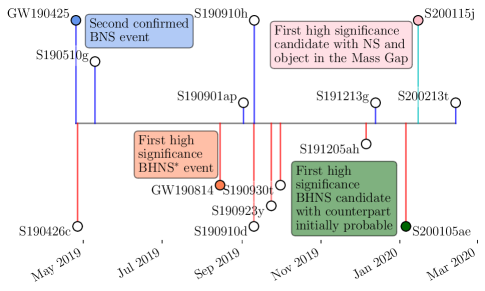
Figure 1: Timeline of O3 alerts with highest probability as being BNS, BHNS or MassGap, with highlights of some of the exceptional candidates released. The candidates, if astrophysical, on the top half of the plot are most likely BNSs (or a NS-MassGap candidate in the case of S200115j (LIGO Scientific Collaboration & Virgo Collaboration, 2020e)), while the candidates on the bottom half are most likely BHNSs. We highlight GW190425 (Abbott et al., 2020b), GW190814 (Abbott et al., 2020a), S200105ae (LIGO Scientific Collaboration & Virgo Collaboration, 2020a, d), and S200115j (LIGO Scientific Collaboration & Virgo Collaboration, 2020e). We note that the initial estimate of p(remnant) for S200105ae was 12% (LIGO Scientific Collaboration & Virgo Collaboration, 2020a), but is now $<$ 1% (LIGO Scientific Collaboration & Virgo Collaboration, 2020d). It also has a significance likely greatly underestimated due to it being a single-instrument event, and a chirp-like structure in the spectrograms as mentioned in the public reports (LIGO Scientific Collaboration & Virgo Collaboration, 2020a, b).
^∗We note that GW190814 contains either the highest mass neutron star or lowest mass black hole known (Abbott et al., 2020a).

Despite those observational difficulties, the O3a and O3b observational campaigns were popular for searches of EM counterparts associated with the GW candidates (see Figure 1 for a timeline for candidates with at least one NS component expected). They mobilized $\sim$ 100 groups covering multiple messengers, including neutrinos, cosmic rays, and the EM spectrum; about half of the participating groups are in the optical. In total, GW follow-up represented $\sim$ 50% of the GCN service traffic (Gamma-ray Coordinates Network) with 1,558 circulars. The first half of the third observation run (O3a) brought ten compact binary merger candidates that were expected to have low-mass components, including GW190425 (LIGO Scientific Collaboration & Virgo Collaboration, 2019b, c), S190426c (LIGO Scientific Collaboration & Virgo Collaboration, 2019d, f), S190510g (LIGO Scientific Collaboration & Virgo Collaboration, 2019e), GW190814 (Abbott et al., 2020a), S190901ap (LIGO Scientific Collaboration & Virgo Collaboration, 2019g), S190910h (LIGO Scientific Collaboration & Virgo Collaboration, 2019i), S190910d (LIGO Scientific Collaboration & Virgo Collaboration, 2019h), S190923y (LIGO Scientific Collaboration & Virgo Collaboration, 2019j), and S190930t (LIGO-Virgo collaboration, 2019). The follow-up campaigns of these candidates have been extensive, with a myriad of instruments and teams scanning the sky localizations.

The follow-up of O3a yielded a number of interesting searches. For example, GW190425 (Abbott et al., 2020b) brought stringent limits on potential counterparts from a number of teams, including GROWTH (Coughlin et al., 2019d) and MMT/SOAR (Hosseinzadeh et al., 2019). GW190814, as a potential, well-localized BHNS candidate, also had extensive follow-up from a number of teams, including GROWTH (Andreoni et al., 2020a), ENGRAVE (Ackley et al., 2020), GRANDMA (Antier et al., 2019) and Magellan (Gomez et al., 2019). S190521g brought the first strong candidate counterpart to a BBH merger Graham et al. (2020).

The second half of the third observation run (O3b) has brought 23 new publicly announced compact binary merger candidates for which observational facilities performed follow-up searches, including two new BNS candidates, S191213g (LIGO Scientific Collaboration & Virgo Collaboration, 2019l) and S200213t (LIGO Scientific Collaboration & Virgo Collaboration, 2020g) and two new BHNS candidates, S191205ah (LIGO Scientific Collaboration & Virgo Collaboration, 2019k) and S200105ae (LIGO Scientific Collaboration & Virgo Collaboration, 2020a, d). S200115j is special for having one NS component and one component object likely falling in the “MassGap” regime, indicating it is between 3–5 M_⊙(LIGO Scientific Collaboration & Virgo Collaboration, 2020e). After the second half of this intensive campaign, no significant counterpart (either GRB or kilonovae) was found. While this might be caused by the fact that the GW triggers have not been accompanied by bright EM counterparts, a likely reason for this lack of success in finding optical counterparts is the limited coordination of global EM follow-up surveys and the limited depth of the individual observations.

In this article, we build on our summary of the O3a observations (Coughlin et al., 2019c) to explore constraints on potential counterparts based on the wide field-of-view telescope observations during O3b, and provide analyses summarizing how we may improve existing strategies with respect to the fourth observational run of advanced LIGO and advanced Virgo (O4). In Sec. 2, we review the optical follow-up campaigns for these sources. In Sec. 3, we summarize parameter constraints that are possible to achieve based on these follow-ups assuming that the candidate location was covered during the observations. In Sec. 4, we use the results of these analyses and others to inform future observational strategies trying to determine the optimal balance between coverage and exposure time. Finally, in Sec. 5, we summarize our findings.

2 EM follow-up campaigns

Table 1: Current overview of non-retracted GW triggers with large probabilities of being BNS or BHNS systems. The individual columns refer to: The name of the event, an estimate using the most up-to-date classification for the event to be a BNS [p(BNS)], a BHNS [p(BHNS)], or terrestrial noise [p(terrestrial)] (Kapadia et al., 2020), and an indicator to estimate the probability of producing an EM signature assuming the candidate is of astrophysical origin [p(HasRemnant)] (Chatterjee et al., 2019), whose definition is in the LIGO-Virgo alert userguide. Note that S200115j can also be classified as “MassGap,” completing the possible classifications. During O3b, a change in the template bank used led to a simplified version of the classification scheme where all of the astrophysical probabilities but one became 0, whereas during O3a, accounting for the mass uncertainty, more than one non-zero astrophysical class probability was generally obtained.

Name	p(BNS)	p(BHNS)	p(terr.)	p(HasRemn.)
S191205ah	$0\%$	$93\%$	$7\%$	$<1\%$
S191213g	$77\%$	$<1\%$	$23\%$	$>99\%$
S200105ae	$0\%$	$3\%$	$97\%$	$<1\%$
S200115j	$<1\%$	$<1\%$	$<1\%$	$>99\%$
S200213t	$63\%$	$<1\%$	$37\%$	$>99\%$

S200115j                                                                    S200213t

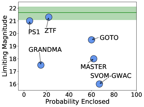
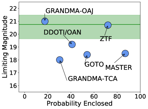
Figure 2: Comparison of limiting magnitudes and probabilities covered for S200115j (left) and S200213t (right). Observations span from immediately post merger up to a week after the GW trigger time. As a point of reference, we include as a green solid line, the apparent magnitude of an object with an absolute magnitude of $-16$, i.e., consistent with a signal similar to AT2017gfo. The green shaded region incorporated the $\pm$ 1 $\sigma$ error bar of the distance that agrees with the two events.

We summarize the EM follow-up observations of the various teams that performed synoptic coverage of the sky localization area and circulated their findings in publicly available circulars during the second half of Advanced LIGO and Advanced Virgo’s third observing run. The LIGO-Scientific and Virgo collaborations used the same near-time alert system during O3b as during O3a, releasing alerts within 2–6 minutes in general (with an important exception, S200105ae, discussed below). For a summary of the second observing run, please see Abbott et al. (2019d), and for the first six months of the third observing run, see Coughlin et al. (2019c) and references therein. In addition to the classifications for the event in categories BNS, BHNS, “MassGap,” or terrestrial noise (Kapadia et al., 2020) and an indicator to estimate the probability of producing an EM signature assuming the candidate is of astrophysical origin, p(HasRemnant) (Chatterjee et al., 2019), skymaps using BAYESTAR (Singer et al., 2014) are also released. At later times, updated LALInference (Veitch et al., 2015) skymaps are also sent to the community.

In addition to the summaries below, we provide Table 1, displaying source properties based on publicly available information in GCNs and Table 2, displaying the results of follow-up efforts for the relevant candidates. All numbers listed regarding coverage of the localizations refer explicitly to the 90% credible region. We treat S200115j as a BHNS candidate despite its official classification as a “Mass-Gap” event; it has p(HasRemnant) value close to 1, indicating the presence of a NS, but with a companion mass between 3 and 5 solar masses. In addition, we compare the limiting magnitudes and probabilities covered for S200115j and S200213t in Figure 2, highlighted as example BHNS and BNS candidates with deep limits from a number of teams. As a point of reference, we include the apparent magnitude of an object with an absolute magnitude of $-16$ with distances ($\pm$ 1 $\sigma$ error bars) consistent with the respective events. As a more physical visualization of the coordinated efforts that go into the follow-up process, we provide Figure 3; this representation displays the tiles observed by various telescopes for the BNS merger candidate S200213t, along with a plot of the integrated probability and sky area that was covered over time by each of the telescopes. The black line is the combination of observations made by the telescopes indicated in the caption. These plots are also reminiscent of public, online visualization tools such as GWSky, the Transient Name Server (TNS), and the Gravitational Wave Treasure Map (Wyatt et al., 2020).

S200115j                                                                    S200213t
Within 12 hours of merger

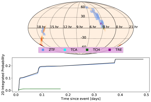
Within 24 hours of merger

Within 48 hours of merger

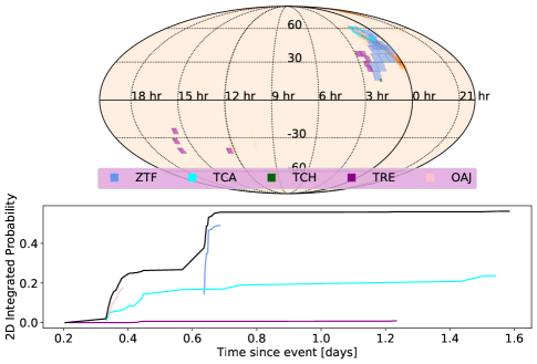
Figure 3: Coverage of the neutron star - black hole candidate S200115j (left column) and binary neutron star candidate S200213t (right column) within 12 hr (top row), 24 hr (middle row), and 48 hr (bottom row) after the GW trigger time by ZTF (Bhalerao et al., 2020; Kasliwal et al., 2020b) and GRANDMA, including the TAROT (TCA, TCH and TRE) network and OAJ (Antier et al., 2020). The LALInference localization probabilites are shown in shaded red. S200115j was detected at 2020-01-15 04:23:09.742 UTC, enabling immediate follow-up observations in South and North America (TCH and ZTF). S200213t was detected at 2020-02-13 at 04:10 UTC, offering only a few hours of observation for the European telescopes, such as for TCA, but a full night of observations with ZTF. OAJ could have begun observing immediately post-merger, but technical issues required human intervention and so the observations began only a few hours post-merger. We plot the integrated probability covered in the 2D skymap with solid lines. We show all telescopes combined in the black lines. The full list of observations is reported in Table 2.

2.1 S191205ah

LIGO/Virgo S191205ah was identified by the LIGO Hanford Observatory (H1), LIGO Livingston Observatory (L1), and Virgo Observatory (V1) at 2019-12-05 21:52:08 UTC (LIGO Scientific Collaboration & Virgo Collaboration, 2019k) with a false alarm rate of one in two years. It has been so far categorized as a BHNS signal $(93\%)$ with a small probability of being terrestrial $(7\%)$. The distance is relatively far at $385\pm 164$ Mpc, and the event localization is coarse, covering nearly $6400$ square degrees. No update of the sky localisation and alert properties have been released by the LVC.

23 groups participated in the follow-up of the event including 3 neutrinos observatories (including IceCube and ANTARES; Ageron et al. 2019; Hussain et al. 2019), two VHE $\gamma$-ray observatories, eight $\gamma$-ray instruments, two X-ray telescopes and ten optical groups (see the list of GCNs for S191205ah). No candidates were found for the neutrinos, high-energy and $\gamma$-ray searches. Five of the optical groups have been engaged for the search of EM counterparts: GRANDMA network, MASTER network, SAGUARO, SVOM-GWAC, and the Zwicky Transient Facility (see Table 2). The MASTER-network led the way in covering a significant fraction of the localization area, observing $\approx 56$% down to 19 in a clear filter and within 144 h (Lipunov et al., 2019i). Seven transient candidates were reported by the Zwicky Transient Facility (Andreoni et al., 2019b), as well as four transient candidates reported by Gaia (Eappachen et al., 2019), and one candidate from the SAGUARO Collaboration (Paterson et al., 2019), although none displayed particularly interesting characteristics encouraging further follow-up; all of the candidates for which spectra were obtained were ultimately ruled out as unrelated to S191205ah (Castro-Tirado et al., 2019a, b, c).

2.2 S191213g

LIGO/Virgo S191213g was identified by H1, L1, and V1 at 2019-12-13 04:34:08 UTC (LIGO Scientific Collaboration & Virgo Collaboration, 2019l). It has been so far categorized as a BNS signal $(77\%)$ with a moderate probability of being terrestrial $(23\%)$, as well as a note that scattered light glitches in the LIGO detectors may have affected the estimated significance and sky position of the event. As expected for BNS candidates, the distance is more nearby (initially $195\pm 59$ Mpc, later updated to be $201\pm 81$ Mpc with the LALInference map LIGO Scientific Collaboration & Virgo Collaboration 2019n). The updated map covered $\sim 4500$ square degrees. Since the updated skymap was released $\sim$ 1 day after trigger time, much of the observations made in the first night used the initial BAYESTAR map.

While it was the first BNS alert during the second half of the O3 campaign, the response to this alert was relatively tepid, likely due to the scattered light contamination. However, 53 report circulars have been distributed for this event due to the presence of an interesting transient found by the Pan-STARRS Collaboration PS19hgw/AT2019wxt, finally classified as supernovae IIb due to the photometry evolution and spectroscopy characterization (McBrien et al., 2019b; Vallely, 2019; Antier et al., 2020). In total, three neutrinos, one VHE, eight $\gamma$-rays, two X-rays, 19 optical and one radio groups participated to the S191213g campaign (see the list of GCNs for S191213g). No significant neutrino, VHE and $\gamma$-ray GW counterpart was found in the archival analysis. A moderate fraction of the localization area was covered using a tiling approach (GRANDMA, Master-Network, ZTF) (see Table 2). The MASTER-network covered $\approx 41$% within 144 h down to 19 in clear (Lipunov et al., 2019j), and the Zwicky Transient Facility covered $\approx 28$% down to 20.4 in $g$- and $r$-band (Andreoni et al., 2019c; Stein et al., 2019c; Kasliwal et al., 2020a). The search yielded 19 candidates of interest from ZTF, as well as the transient counterpart AT2019wxt from the Pan-STARRS Collaboration (McBrien et al., 2019b). It was shown that all ZTF candidates were in fact unrelated with the GW candidate S191213g (Perley & Copperwheat, 2019; Brennan et al., 2019; Andreoni et al., 2019d).

In addition to searches by wide field of view telescopes, there was also galaxy-targeted follow-up performed by the J-GEM Collaboration, observing 57 galaxies (Onozato et al., 2019), and the GRANDMA citizen science program, observing 16 galaxies (Ducoin et al., 2019) within the localization of S191213g.

2.3 S200105ae

LIGO/Virgo S200105ae was identified by L1 (with V1 also observing) at 2020-01-05 16:24:26 UTC as a subthreshold event with a false alarm rate of 24 per year; if it is astrophysical, it is most consistent with being an BHNS. However, its significance is likely underestimated due to it being a single-instrument event. This candidate was most interesting due to the presence of chirp-like structure in the spectrograms (LIGO Scientific Collaboration & Virgo Collaboration, 2020a, b). The first public notice was delivered 27.2 h after the GW trigger impacting significantly the follow-up campaign of the event. In addition, the most updated localization was very coarse, spanning $\sim 7400$ square degrees with a distance of $283\pm 74$ Mpc (LIGO Scientific Collaboration & Virgo Collaboration, 2020d).

S200105ae follow-up activity was comparable to S191205ah’s: 25 circular reports were associated to the S200105ae in the GCN service with the search of counterpart engaged by two neutrinos, one VHE, seven $\gamma$-ray, one X-ray and five optical groups (see the list of GCNs for S200105ae). No significant neutrino, VHE and $\gamma$-ray GW counterpart was found in the archival analysis. Various groups participated to the search of optical counterpart with ground-based observatories: GRANDMA, Master-Network, and the Zwicky Transient Facility (see Table 2). The alert space system for Gaia was also activated (Kostrzewa-Rutkowska et al., 2020). The MASTER-network covered $\approx 43$% down to 19.5 in clear and within 144 h (Lipunov et al., 2020a). The telescope network was already observing at the time of the trigger and because its routine observations were compatible with the sky localization of S200105ae, the delay was limited to 3 hr. GRANDMA-TCA telescope was triggered as soon as the notice comes out, and the full GRANDMA network totalized 12.5 % of the full LALInference skymap down to 17 mag in clear and within 60 h (Antier et al., 2020). The Zwicky Transient Facility covered $\approx 52$% of the LALInference skymap down to 20.2 in both $g$- and $r$-bands (Stein et al., 2020; Kasliwal et al., 2020a) and with a delay of 10 h. There were 23 candidate transients reported by ZTF, as well as one candidate from the Gaia Alerts team (Kostrzewa-Rutkowska et al., 2020) out of which ZTF20aaervoa and ZTF20aaertpj were both quite interesting due to their red colors ($g-r$= 0.66 and 0.35 respectively), and absolute magnitudes ($-16.4$ and $-15.9$ respectively) (Stein et al., 2020). ZTF20aaervoa was soon classified as a SN IIp $\sim 3$ days after maximum, and ZTF20aaertpj as a SN Ib close to maximum (Castro-Tirado et al., 2020a, b).

2.4 S200115j

LIGO/Virgo S200115j, a MassGap signal $(99\%)$ with a very high probability $(99\%)$ of containing a NS as well, was identified by H1, L1, and V1 at 2020-01-15 04:23:09.742 UTC (LIGO Scientific Collaboration & Virgo Collaboration, 2020e). As discussed before, it can be considered as a BHNS candidate. Due to its discovery by multiple detectors, the sky location is well-constrained; the most updated map spans $\sim 765$ square degrees, with most of the probability shifting towards the southern lobe in comparison to the initial localization, and has a distance of $340\pm 79$  Mpc.

With a very high p${}_{\mathrm{remnant}}>99$% (LIGO Scientific Collaboration & Virgo Collaboration, 2020f) and good localization, many space and ground instruments/telescopes followed up this signal: 33 circular reports were associated to the event in the GCN service with the search of counterpart engaged by two neutrinos, three VHE, five $\gamma$-ray, two X-ray and eight optical groups (see the list of GCNs for S200115j). INTEGRAL was not active during the time of the event (Ferrigno et al., 2020) and so was unable to report any prompt short GRB emission. No significant neutrino, VHE and $\gamma$-ray GW counterpart was found in the archival analysis. Swift satellite was also pointed toward the best localization region for finding X-ray and UVOT counterpart. Some candidates were reported: one of them was detected in the optical by Swift/UVOT and the Zwicky Transient Facility, but was concluded to likely be due to AGN activity (Oates et al., 2020; Andreoni et al., 2020b).

Various groups participated to the search of optical counterpart with ground observatories: GOTO, GRANDMA, Master-Network, Pan-Starrs, SVOM-GWAC and the Zwicky Transient Facility (see Table 2). GOTO (Steeghs et al., 2020) covered $\approx 50$% down to 19.5 in $G$-band, starting almost immediately the observations, while the SVOM-GWAC team covered $\approx 40$% of the LALInference sky localization down to 16 in R-band using the SVOM-GWAC only 16h after the trigger time (Han et al., 2020).

In addition, a list of 20 possible host galaxies for the trigger was produced by convolving the GW localization with the 2MPZ galaxy catalog (Evans et al., 2020a; Bilicki et al., 2014); 12 of these galaxies were observed by GRAWITA (Savaglio et al., 2020) in the r-sdss filter.

2.5 S200213t

S200213t was identified by H1, L1, and V1 at 2020-02-13 at 04:10:40 UTC (LIGO Scientific Collaboration & Virgo Collaboration, 2020g). It has been categorized as a BNS signal $(63\%)$ with a moderate probability of being terrestrial $(37\%)$. The LALInference localization spanned $\sim 2326$ square degrees, with a distance of $201\pm 80$  Mpc (LIGO Scientific Collaboration & Virgo Collaboration, 2020h). A total of 51 circular reports were associated to this event including two neutrinos, two VHE, eight $\gamma$-rays, two X-ray, and eleven optical groups (see the list of GCNs for S200213t). Fermi and Swift were both transiting the South Atlantic Anomaly at the time of event, and so were unable to observe and report any GRBs coincident with S200213t (Veres et al., 2020; Lien et al., 2020). No significant counterpart candidate was found during archival analysis: IceCube detected muon neutrino events, but it was shown that they have not originated from the GW source (Hussain, 2020).

With a very high p${}_{\mathrm{remnant}}>99$% and probable BNS classification, many telescopes followed-up this signal: DDOTI/OAN, GOTO, GRANDMA, MASTER and ZTF. DDTOI/OAN covered $\approx 40$% of the LALInference skymap starting less than 1h after the trigger time down to 19.2 in $w$-band (Alan et al., 2020), GRANDMA covered 32% of the LALInference area within $\approx$ 26h down to 18 mag in clear (TCA) and down to 21 mag in R-band (OAJ). GOTO covered $\approx 54$% of bayestar skymap down to 18.4 in $G$-band (Cutter et al., 2020). 15 candidate transients were reported by ZTF (Kasliwal et al., 2020b; Andreoni et al., 2020c; Reusch et al., 2020), as well as one by the MASTER-network (Lipunov et al., 2020d). All were ultimately ruled out as possible counterparts to S200213t through either spectroscopy or due to pre-discovery detections (Castro-Tirado et al., 2020c, d; Ho et al., 2020; Andreoni et al., 2020d; Srivastav & Smartt, 2020; Mroz et al., 2020). Galaxy targeted observations were conducted by several observatories: examples include KAIT, which observed 108 galaxies (Zheng et al., 2020), Nanshan-0.6m, which observed a total of 120 galaxies (Xu et al., 2020), in addition to many other teams (Onozato et al., 2020; Gregory, 2020).

3 Kilonova Modeling and possible ejecta mass limits

Following Coughlin et al. (2019c), we will compare the upper limits described in Section 2 to different kilonova models. We seek to measure “representative constraints,” limited by the lack of field and time-dependent limits. To do so, we approximate the upper limits in a given passband as one-sided Gaussian distributions. We take the sky-averaged distance in the GW localizations to determine the transformation from apparent to absolute magnitudes. To include the uncertainty in distance, we sample from a Gaussian distribution consistent with this uncertainty and add it to the model lightcurves. In this analysis, we employ three kilonova models based on Kasen et al. (2017), Bulla (2019), and Hotokezaka & Nakar (2019), in order to compare any potential systematic effects. These models use similar heating rates (Metzger et al., 2010; Korobkin et al., 2012), while using different treatments of the radiative transfer.

                                                                                                                                                                                                                                       Model I                                                         Model II                                                         Model III
S191213g

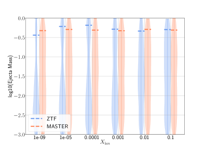
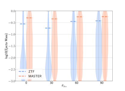
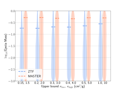
S200213t

Figure 4: Probability density for the total ejecta mass for the BNS events, S191213g and S200213t, and employed lightcurve models. From the left to the right, we show constraints as a function of lanthanide fraction for the Kasen et al. (2017) Model, as a function of inclination angle (from a polar orientation, system viewed face-on) for the Bulla (2019) Model, and as a function of the opacity of the 2-components, $\kappa_{\rm low}$ and $\kappa_{\rm high}$ for the Hotokezaka & Nakar (2019) Model. The dashed lines are the upper limits that contain 90% of the probability density. For S191213g, we use ZTF (Andreoni et al., 2019c; Stein et al., 2019c) and the MASTER-Network (Lipunov et al., 2019j). For S200213t, we use ZTF (Kasliwal et al., 2020b) and GOTO (Cutter et al., 2020). See Table 2 for further details.

Figure 5: Probability density for the total ejecta mass for the NSBH events, S191205ah, S200105ae, and S200115j, and employed lightcurve models. From the left to the right, we show constraints as a function of lanthanide fraction for the Kasen et al. (2017) Model, as a function of inclination angle (from a polar orientation, system viewed face-on) for the Bulla (2019) Model, and as a function of the opacity of the 2-components, $\kappa_{\rm low}$ and $\kappa_{\rm high}$ for the Hotokezaka & Nakar (2019) Model. The dashed lines are the upper limits that contain 90% of the probability density. For S191205ah, we use ZTF (left, Andreoni et al. 2019b) and SAGUARO (right, Paterson et al. 2019). For S200105ae, we use ZTF (Stein et al., 2020) and the MASTER-network (Lipunov et al., 2020a). For S200115j, we use ZTF (Bhalerao et al., 2020) and GOTO (Steeghs et al., 2020) See Table 2 for further details.

Model I                                                         Model II                                                         Model III
S191205ah

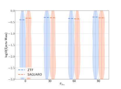
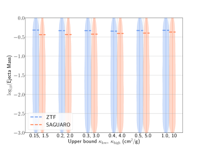
S200105ae

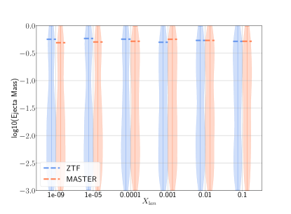
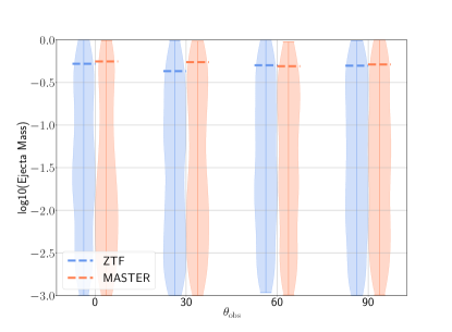
S20015j

 

We will show limits as a function of one parameter for each model chosen to maximize its impact on the predicted kilonova brightness and color, marginalizing out the other parameters when performing the sampling. For the models based on Kasen et al. (2017) and Bulla (2019), as grid-based models, we interpolate these models by creating a surrogate model using a singular value decomposition (SVD) and Gaussian Process Regression (GPR) based interpolation (Doctor et al., 2017) that allows us to create lightcurves for arbitrary ejecta properties within the parameter space of the model  (Coughlin et al., 2019b; Coughlin et al., 2018b). We refer the reader to Coughlin et al. (2019c) for more details about the models, but we will also briefly describe them in the following for completeness.

Model I (Kasen et al., 2017) depends on the ejecta mass $M_{\rm ej}$, the mass fraction of lanthanides $X_{\rm lan}$, and the ejecta velocity $v_{\rm ej}$. We allow the sampling to vary within $-3\leq\log_{10}(M_{\rm ej}/M_{\odot})\leq 0$ and $0\leq v_{\rm ej}\leq 0.3$ $c$, while restricting the lanthanide fraction to $X_{\rm lan}$ = [ $10^{-9}$, $10^{-5}$, $10^{-4}$, $10^{-3}$, $10^{-2}$, $10^{-1}]$.

Model II (Bulla, 2019) assumes an axi-symmetric geometry with two ejecta components, one component representing the dynamical ejecta and one the post-merger wind ejecta. Model II depends on four parameters: the dynamical ejecta mass $M_{\rm ej,dyn}$, the post-merger wind ejecta mass $M_{\rm ej,pm}$, the half-opening angle of the lanthanide-rich dynamical-ejecta component $\phi$ and the inclination angle $\theta_{\rm obs}$ (with $\cos\theta_{\rm obs}=0$ and $\cos\theta_{\rm obs}=1$ corresponding to a system viewed edge-on and face-on, respectively). We refer the reader to Dietrich et al. (2020) for a more detailed discussion of the ejecta geometry. In this study, we fix the dynamical ejecta mass to the best-fit value from Dietrich et al. (2020), $M_{\rm ej,dyn}=0.005\,M_{\odot}$, and allow the sampling to vary within $-3\leq\log_{10}(M_{\rm ej,pm}/M_{\odot})\leq 0$ and $0^{\circ}\leq\phi\leq 90^{\circ}$, while restricting the inclination angle to $\theta_{\rm obs}=[0^{\circ},30^{\circ},60^{\circ},90^{\circ}]$. To facilitate comparison with the other models, we will provide constraints on the total ejecta mass $M_{\rm ej}=M_{\rm ej,dyn}+M_{\rm ej,pm}$ for Model II. We note that the model adopted here is more tailored to BNS than BHNS mergers given the relatively low dynamical ejecta mass, $M_{\rm ej,dyn}=0.005\,M_{\odot}$. However, for a given $M_{\rm ej,pm}$, the larger values of $M_{\rm ej,dyn}$ predicted in BHNS are expected to produce longer lasting kilonovae more easily detectable. Therefore, the ejecta mass upper limits derived below for BHNS systems should be considered conservative.

Model III (Hotokezaka & Nakar, 2019) depends on the ejecta mass $M_{\rm ej}$, the dividing velocity between the inner and outer component $v_{\rm ej}$, the lower and upper limit of the velocity distribution $v_{\text{min}}$ and $v_{\text{max}}$, and the opacity of the 2-components, $\kappa_{\rm low}$ and $\kappa_{\rm high}$. We allow the sampling to vary $-3\leq\log_{10}(M_{\rm ej}/M_{\odot})\leq 0$, $0\leq v_{\rm ej}\leq 0.3$ $c$, $0.1\leq v_{\text{min}}/v_{\text{ej}}\leq 1.0$ and $1.0\leq v_{\text{max}}/v_{\text{ej}}\leq 2.0$. We restrict $\kappa_{\rm low}$ and $\kappa_{\rm high}$ to a set of representative values in the analysis, i.e. 0.15 and 1.5, 0.2 and 2.0, 0.3 and 3.0, 0.4 and 4.0, 0.5 and 5.0, and 1.0 and 10 cm²/g.

Figure 4 shows the ejecta mass constraints for BNS events, S191213g and S200213t, while Figure 5 shows them for NSBH events, S191205ah, S200105ae, and S200115j. We mark each $90\%$ confidence with a horizontal dashed line. As a brief reminder, given that the entire localization region is not covered for these limits, and the limits implicitly assume that the region containing the counterpart was imaged, these should be interpreted as optimistic scenarios. It is also simplified to assume that the light curve can not exceed the stated limit at any point in time. Similar to what was found during the analysis of O3a (Coughlin et al., 2019c), the constraints are not particularly strong, predominantly due to the large distances for many of the candidate events. Given the focus of these systems on the bluer optical bands, the constraints for the bluer kilonova models (low $X_{\rm lan}$, low $\theta_{\rm obs}$ and low $\kappa_{\rm low}/\kappa_{\rm high}$) tend to be stronger.

S191205ah: The left column of Figure 5 shows the ejecta mass constraints for S191205ah based on observations from ZTF (left, Andreoni et al. 2019b) and SAGUARO (right, Paterson et al. 2019). For all models we basically recover our prior, i.e., no constraint on the ejecta mass can be given.

S191213g: The middle column of Figure 4 shows the ejecta mass constraints for S191213g based on the observations from ZTF (Andreoni et al., 2019c; Stein et al., 2019c) and the MASTER-Network (Lipunov et al., 2019j). Interestingly, Model II allows us for small values of $\theta_{\rm obs}$ (brighter kilonovae) to constrain ejecta masses above $\sim 0.3$ $M_{\odot}$, however for larger angles, no constraint can be made. For Model III we obtain even tighter ejecta mass limits between $0.2$ $M_{\odot}$ and $0.3$ $M_{\odot}$, where generally for potentially lower opacity ejecta we obtain better constraints. While $0.2$ $M_{\odot}$ rules out systems producing very large ejecta masses, e.g., highly unequal mass systems, AT2017gfo was triggered by only about a quarter of the ejecta mass and our best bound for GW190425 (Coughlin et al., 2019c) was a factor of a few smaller. Thus, we are overall unable to extract information that help us to constrain the properties of the GW trigger S191213g.

S200105ae: The right column of Figure 5 shows the ejecta mass constraints for S200105ae based on observations from ZTF (Stein et al., 2020) and the MASTER-network (Lipunov et al., 2020a). As for S191205ah our analysis recovers basically the prior and no additional information can be extracted.

S200115j: The left column of Figure 5 shows the ejecta mass constraints for S200115j based on observations from ZTF (Bhalerao et al., 2020) and GOTO (Steeghs et al., 2020). Model II allows us for small values of $\theta_{\rm obs}$ (brighter kilonovae) to constrain ejecta masses above $\sim 0.1$ $M_{\odot}$, however for larger angle, no constraint can be made; similar constraints (ejecta masses below $0.15$ $M_{\odot}$) are also obtained with Model III. As for S191213g, the obtained bounds are not strong enough to reveal interesting properties about the source properties.

S200213t: The right column of Figure 4 shows the ejecta mass constraints for S200213t based on observations from ZTF (Kasliwal et al., 2020b) and GOTO (Cutter et al., 2020). As for S191205ah and S191213g, our analysis recovers basically the prior and no additional information can be extracted for Model I and Model II. Model III allows us to rule out large ejecta masses $>0.15$ $M_{\odot}$ for low opacities.

Summary: In conclusion, we find that for the follow-up surveys to the important triggers of O3b, the derived constraints on the ejecta mass are too weak to extract any information about the sources as it was possible for GW190425 (Coughlin et al., 2019c). This is likely due to a number of different circumstances: a reduction number of observations from O3a to O3b, e.g., three GW events out of five were happening around 4 h UTC, leading to an important delay of observations for all facilities located in Asia and Europe. Furthermore, the distance to most of the events was quite far (around 200 Mpc) and there was the possibility that in many cases a non-astrophysical origin caused the GW alert. Also, the weather was particularly problematic for a number of the promising events (see above). Unfortunately, we also observed that some groups were less rigorous in their report compared to O3a and did not report all observations publicly, which clearly hinders the analysis outlined above. Overall, some of the observational strategies were not optimal and motivates a more detailed discussion in Section 4.

While these analyses do not evaluate the joint constraints possible based on multiple systems, under the assumption that different telescopes observed the same portion of the sky in different bands (or at different times), it makes sense that improved constraints on physical parameters are possible. To demonstrate this, we show the ejecta mass constraints for GW190425 based on observations from ZTF (left, Kasliwal et al. (2019a)) and PS1 (right, Smith et al. (2019)) and the combination of the two. While the constraints for the low lanthanide fractions are stronger than available for the “red kilonovae” for all examples, the combination of $g$- and $r$-band observations from ZTF and $i$-band from PS1 yield stronger constraints across the board.

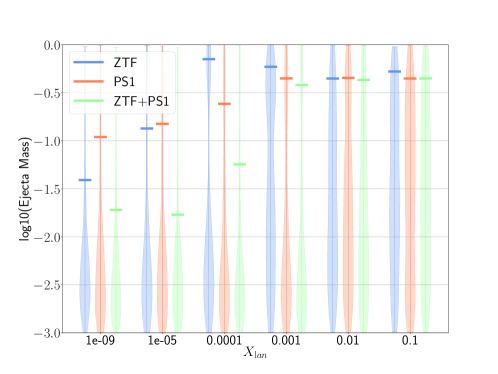
Figure 6: Probability density for the total ejecta mass for GW190425 based on the Kasen et al. (2017) model using the ZTF (left, Kasliwal et al. (2019a)), PS1 (right, Smith et al. (2019)), and joint ZTF and PS1 limits.

4 Using the kilonova models to inform observational strategies

OAJ                                                                    PS1

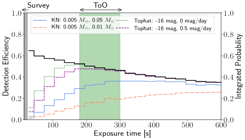
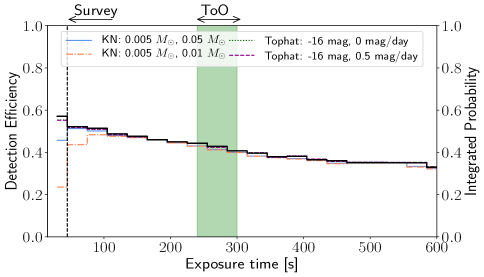
ZTF                                                             ZTF+PS1+OAJ

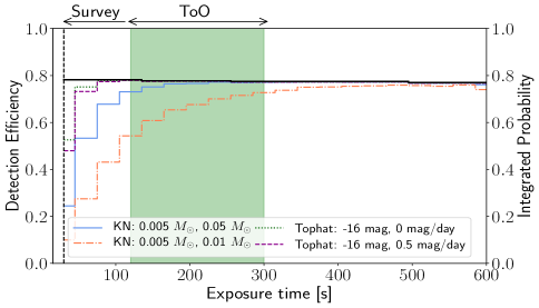
Figure 7: Efficiency of recoveries for S200213t (focusing on $g$- and $r$-band observations). We include a model with a constant absolute magnitude of $-16$ with 0 mag/day-decay, a model with a base absolute magnitude of $-16$ and decay rate of 0.5 mag/day, and two kilonova models (Bulla, 2019), one with dynamical ejecta of $M_{\rm ej,dyn}=0.005\,M_{\odot}$ and post-merger wind ejecta $M_{\rm ej,pm}=0.01\,M_{\odot}$ and the other one with $M_{\rm ej,dyn}=0.005\,M_{\odot}$ and $M_{\rm ej,pm}=0.05\,M_{\odot}$. We show the integrated probability of the most updated sky localization area of S200213t covered by observations made within 72 hours of the event in a solid black line; we note that this is the same integrated probability for the schedule in all four models, and the detection efficiency and integrated probability should converge to the same values in cases where all kilonovae within a specific portion of the 2-D localization are detectable. The maximum coverage reachable for the three sites is 65% for OAJ, 78% for ZTF, 57% for PS1, and 88% for the network. We also show the nominal survey exposure times in vertical dashed lines (for OAJ, we show a gray band indicating the range of survey times employed, which changes based on atmospheric and moon conditions) and range of ToO observation exposure times (120-300 s) for comparison. We include analyses using OAJ (top left), PS1 (top right), ZTF (bottom left) individually, and a joint analysis of the three.

Given the relatively poor limits on the ejecta masses, we are interested in understanding how optimized scheduling strategies can aid in obtaining higher detection efficiencies of kilonova counterparts. Similar but slightly stronger constraints were obtained during the analysis of the first six months of O3 (Coughlin et al., 2019c), where we advocated for longer observations at the cost of a smaller sky coverage.

For our investigation, we use the codebase gwemopt (Gravitational-Wave ElectroMagnetic OPTimization) (Coughlin et al., 2018a), which has been developed to schedule Target of Opportunity (ToO) telescope observations after the detection of possible multi-messenger signals, including neutrinos, gravitational waves, and $\gamma$-ray bursts. There are three main aspects to this scheduling: tiling, time allocation, and scheduling of the requested observations. Multi-telescope, network-level observations (Coughlin et al., 2019a) and improvements for scheduling in the case of multi-lobed maps (Almualla et al., 2020) are the most recent developments in these areas. We note that gwemopt naturally accounts for slew and read out times based on telescope-specific configuration parameters, which are important to account for inefficiencies in either long slews or when requesting short exposure times.

We now perform a study employing these latest scheduling improvements to explore realistic schedules, analyzing them with respect to exposure time in order to determine the time-scales required to make kilonova detections. We will use four different types of lightcurve models to explore this effect. The first is based on a “top hat” model, where a specific absolute magnitude is taken as constant over the course of the observations; in this paper, we take an absolute magnitude (in all bands) of $-16$, which is roughly the peak magnitude of AT2017gfo (Arcavi et al., 2017). The second is similar: a base absolute magnitude of $-16$ is taken at the start of observation, but the magnitude decays linearly over time at a decay rate of 0.5 mag/day. These agnostic models depend only on the intrinsic luminosity and luminosity evolution of the source. The third and fourth model types are derived from our Model II (Bulla, 2019). We use two different values of the post-merger wind ejecta component to explore the dependence on the amount of ejecta, one with dynamical ejecta $M_{\rm ej,dyn}=0.005\,M_{\odot}$ and post-merger wind ejecta $M_{\rm ej,pm}=0.01\,M_{\odot}$ and the other with $M_{\rm ej,dyn}=0.005\,M_{\odot}$ and $M_{\rm ej,pm}=0.05\,M_{\odot}$, similar to that found for AT2017gfo (Dietrich et al., 2020). As mentioned in Section 3, dynamical ejecta masses of $M_{\rm ej,dyn}=0.005\,M_{\odot}$ are more typical for BNS than BHNS mergers, and therefore we restrict our analysis to a BNS event (see below).

Figure 7 shows the efficiency of transient discovery for these models as a function of exposure time for a BNS event occurring at a distance similar to that of S200213t, 224 $\pm$ 90 Mpc. We inject kilonovae according to the 3D probability distribution in the final LALInference localization of S200213t and generate a set of tilings for each telescope (with fixed exposure times) through scheduling algorithms. Here, the detection efficiency corresponds to the total number of detected kilonovae divided by the total number of simulated kilonovae, which is a proxy for the probability that the telescope covered the correct sky location during observations to a depth sufficient to detect the transient.

We show the total integrated probability that the event was part of the covered sky area as a black line, and the probabilities for all four different lightcurve models as colored lines. For our study, we use OAJ (top left), PS1 (top right), and ZTF (bottom left), and a network consisting of all three telescopes. As expected, there is a trade-off between exposure time and the ability to effectively cover a large sky area. Both of these contribute to the overall detection efficiency, given that the depths required for discovery are quite significant. In order to rule out moving objects (e.g., asteroids) during the transient-filtering process, it is important to have at least 30  min gaps between multi-epoch observations; opting for longer exposure times can render this close to impossible, and hinder achieving coverage of the 90% credible region during the first 24 hours, especially for larger localizations. There are also observational difficulties, as field star-based guiding is not available on all telescopes, so some systems are not able to exceed exposure durations of a few minutes without sacrificing image quality. Therefore, we are interested in pinpointing the approximate peaks in efficiency so as to find a balance between the depth and coverage attained, and ultimately increase the possibility of a kilonova detection. It is important to note that the comparably “close” distance of S200213t (listed in Section 2) must be taken into account in this analysis, as farther events will likely favor relatively longer exposure times to achieve the depth required. In addition to exposure time, visibility constraints also contribute to the maximum probability coverage observable from a given site.

Only taking into consideration the single-telescope observations shown in Figure 7, we find that as expected, the peak differs considerably depending on the telescope, by virtue of its configuration. The results with PS1, for example, are illustrative of its lower field of view in combination with its higher limiting magnitude of 21.5 (assuming optimal conditions), leading to both a quick decline in coverage for longer exposure times, and sufficient depth achieved at shorter exposure times. As a result, the efficiency peaks at a much earlier range of $\sim$ 30-100s for this event. In the case of OAJ, the similar field of view to PS1 but relatively lower limiting magnitude supports opting for exposure times of $\sim$ 160 - 300s —in which one expects to reach $\sim$ 20.8 - $\sim$ 21.5 mag— to not lose out on coverage to the point of jeopardizing the detection efficiency for this skymap. ZTF’s 47-square-degree field of view, however, allows for longer exposure times to be explored while maintaining an increase in efficiency. Generally, ZTF ToO follow-ups have used $\sim$ 120 - 300 s exposures (Coughlin et al., 2019d), expected to reach $\sim$ 21.5 $-$ $\sim$ 22.4 mag, but going for even longer exposure times appears beneficial to optimizing counterpart detection for ZTF. The bottom right panel, which shows the joint analysis, aptly re-emphasizes the potential benefit of multi-telescope coordination through the gain in detection efficiency due to the ability to more effectively cover a large sky area; additionally, since achieving significant coverage is no longer an issue, pushing for longer exposure times will only positively affect the chances of detecting a transient counterpart.

As grounds for comparison, we also performed identical simulations for BNS event GW190425 (LIGO Scientific Collaboration & Virgo Collaboration, 2019c) (with a sizable updated localization of $\sim$ 7500 square degrees) in order to investigate the effects of the skymap’s size on the peak efficiencies and the corresponding exposure times. The results are compared using a single telescope configuration (ZTF) vs. a multi-telescope configuration (ZTF, PS1, and OAJ) for different lightcurve models. For the Tophat model with a decay rate of 0.5 mag/day, the detection efficiency peaked at $\sim$ 70s for ZTF, with both the integrated probability and detection efficiency at 27%. However, under identical conditions, the telescope network configuration peaked at a detection efficiency and integrated probability of 34% at $\sim$ 40s. Using the synthetic lightcurve adopted from Model II, with dynamical ejecta of $M_{\rm ej,dyn}=0.005\,M_{\odot}$ and post-merger wind ejecta of $M_{\rm ej,pm}=0.01\,M_{\odot}$, ZTF attained a peak efficiency of 25% at $\sim$ 170s. On the other hand, the telescope network resulted in a higher detection efficiency of 29% at $\sim$ 100s due to the increased coverage. It is clear that regardless of the model adopted, there is some benefit in utilizing telescope networks to optimize the search for counterparts, especially in the case of such large localizations; however, truly maximizing this benefit requires the ability to optimize exposure times on a field-by-field (or at least, telescope-by-telescope) basis. This also requires that the telescopes coordinate their observations, or in other words, optimize their joint observation schedules above and beyond optimization of individual observation schedules.

Figure 8: Efficiency of recoveries for S200213t for a model with a constant absolute magnitude of $-16$ (Tophat), a model with a base absolute magnitude of $-16$ and decay rate of 0.5 mag/day (Tophat), and two kilonova models (Bulla, 2019), one with dynamical ejecta $M_{\rm ej,dyn}=0.005\,M_{\odot}$ and post-merger wind ejecta $M_{\rm ej,pm}=0.01\,M_{\odot}$ and the other one with $M_{\rm ej,dyn}=0.005\,M_{\odot}$ and $M_{\rm ej,pm}=0.05\,M_{\odot}$, similar to that found for AT2017gfo (Dietrich et al., 2020). We also show the nominal ZTF survey exposure time (30 s) and range of ToO observation exposure times (120-300 s) for comparison. On the left is for a limiting magnitude of 20.5, corresponding to 16th percentile night, while on the right, the limiting magnitude is 19.5, corresponding to a 84th percentile night.

Finally, we want to show the impact of observation conditions on the peak detection efficiencies and the corresponding exposure times in Fig. 8. We uses two baselines for ZTF magnitude limits, with one corresponding to 19.5, the median $-1\sigma$ and the other to 20.5, the median $+1\sigma$. Our analysis shows that for good conditions (left panel), the performance for ToOs is reasonable, although especially optimal towards the upper end of the 120 - 300 s range. For relatively poor conditions (right panel), longer exposure times are required, which is now possible due to the significant work that has gone into improving ZTF references to adequate depths for these deeper observations. One more point of consideration is the distance information for the event; a kilonova with twice the luminosity distance will produce four times less flux, and this will affect the depth required to possibly detect the transient. This aspect of the analysis does not overshadow the importance of prioritizing longer exposure times (in particular under bad observational conditions). We note that the quoted limits for S200213t are $\sim$ 20.7 mag in 120 s from ZTF (Kasliwal et al., 2020b); this corresponds to $\sim$ 19.2 expected for 30 s exposures, and therefore sub-optimal conditions.

5 Summary

In this paper, we have presented a summary of the searches for EM counterparts during the second half of the third observing run of Advanced LIGO and Advanced Virgo; we focus on the gravitational-wave event candidates which are likely to be the coalescence of compact binaries with at least one neutron star component. We used three different, independent kilonova models Kasen et al. (2017); Bulla (2019); Hotokezaka & Nakar (2019) to explore potential ejecta mass limits based on the non-detection of kilonova counterparts of the five potential GW events S191205ah, S191213, S200105ae, S200115j, and S200213t by comparing apparent magnitude limits from optical survey systems to the gravitational-wave distances. While the models differ in their radiative transfer treatment, our results show that the publicly-available observations do not provide any strong constraints on the quantity of mass ejected during the possible events, assuming the source was covered by those observations. The most constraining measurement is obtained for S200115j thanks to the observations of ZTF and GOTO; the model of Bulla (2019) excludes an ejecta of more than 0.1 $M_{\odot}$ for some viewing angles. In general, the reduced number of observations between O3a and O3b, the delay of observations, the shallower depth of observations, and large distances of the candidates, which yield faint kilonovae, explain the minimal constraints for the compact binary candidates. However, it shows the benefit of a systematic diagnostic about quantity of ejecta thanks to the observations, as was done in the analysis of O3a (Coughlin et al., 2019c). Although the strategy of follow-up employed by the various teams and their instrument capabilities did not evolve significantly in the eleven months of O3, it is clear that a global coordination of the observations would yield expected gains in efficiency, both in terms of coverage and sensitivity.

Given the uninformative constraints, we explored the depths that would be required to improve the detection efficiencies at the cost of coverage of the sky location areas for both single telescopes and network level observations. We find that exposure times of $\sim$ 3-10 min would be useful for ZTF to maximize its sensitivity for the events discussed here, depending on the model and atmospheric conditions, which is a factor of 6-20 $\times$ longer than survey observations, and up to a factor of 2 $\times$ longer than for current ToO observations; the result is similar for OAJ. For PS1, on the other hand, its larger aperture leads to the conclusion that its natural survey exposure time is about right for events in the BNS distance range. Our results also highlight the advantages of telescope networks in increasing coverage of the localization and thereby allowing for longer exposure times to be used, thus leading to a corresponding increase in detection efficiencies.

It is also important to connect our results to conclusions drawn in other works: Carracedo et al. 2020 showed that detections of a AT2017gfo-like light curve at 200 Mpc requires observations down to limiting magnitudes of 23 mag for lanthanide-rich viewing angles and 22 mag for lanthanide-free viewing angles. The authors point out that because the optical lightcurves of kilonovae become red in a matter of few days, observing in red filters, such as inclusion of $i$-band observations, results in almost double the detections as compared to observations in $g$- and $r$-band only. They propose that observations of rapid decay in blue bands, followed by longer observations in redder bands is therefore an ideal strategy for searching for kilonovae. This strategy can be combined with the exposure time measurements here to create more optimized schedules. Kasliwal et al. 2020a also demonstrate that under the assumption that the GW events are astrophysical, strong constraints on kilonova luminosity functions are possible by taking multiple events and considering them together, even when the probabilities and depths covered on individual events are not always strong. This motivates future work where ejecta mass constraints can be made on a population basis by considering the joint constraints over all events.

Building in field-dependent exposure times will be critical for improving the searches for counterparts. While our estimates are clearly model dependent (e.g., by assuming an absolute magnitude, a decay rate for candidate counterparts, and a particular kilonova model), it is clear that deeper observations are required, especially with the future upgrades of the GW detectors, to improve detection efficiencies when the localization area and telescope configuration allow for it. Telescope upgrades alone do not guarantee success, as detecting more marginal events at further distances will not necessarily yield better covered skymaps. Smaller localizations from highly significant, nearby events are key, perhaps with the inclusion of more information to differentiate those most likely to contain counterpart, such as the chirp mass (Margalit & Metzger, 2019), to support the follow-up.

Data Availability

The data underlying this article are derived from public code found here: https://github.com/mcoughlin/gwemlightcurves. The simulations resulting will be shared on reasonable request to the corresponding author.

Table 2: Reports of the observations by various teams of the sky localization area of gravitational-wave alerts of possible BNS candidates S191213g and S200213t, and BHNS candidates S191205ah, S200105ae, and S200115j. For ease of comparison to limits, assuming an absolute magnitude of $-$16 mag, the median distances correspond to apparent magnitudes of 20.5, 20.5, 21.9, 21.3, and 21.7 mag respectively. Teams that employed “galaxy targeting”during their follow-up or with less than 1% coverage of the sky localisation area are not mentioned here. In the case where numbers were not reported or provided upon request in order to calculate the total coverage based on the most updated sky localization area, we recomputed some of them; if this was not possible, we add $-$.

Telescope	Filter	Limit mag	Delay aft. GW	Duration	GW sky localization area		reference
			(h)	(h)	name	coverage (%)
S191205ah (BHNS)
GRANDMA-TCA	Clear	$18$	$18.9$	$50$	bayestar ini	$3$	Antier et al. (2020)
GRANDMA-TCH	Clear	$18$	$2.9$	$54$	bayestar ini	$1$	Antier et al. (2020)
MASTER-network	Clear	$\approx 19$	$\approx 0.1$	$144$	bayestar ini	$\approx 56$	Lipunov et al. (2019i)
SAGUARO	G-band	$21.3$	4.4	$0.5$	bayestar ini	$9$	Paterson et al. (2019); Wyatt et al. (2020), this work
SVOM-GWAC	R-band	$16$	$\approx 0.1$	$23$	bayestar ini	$28$	Duque et al. (2019), this work
Zwicky Transient Facility	g/r-band	$17.9$	$10.7$	$167$	bayestar ini	$6$	Andreoni et al. (2019b); Kasliwal et al. (2020a)
S191213g (BNS)
GRANDMA-TCA	Clear	$18$	$47.6$	$73$	LALInference	$1$	Antier et al. (2020)
MASTER-network	Clear	$\approx 18.5$	$0.4$	$144$	LALInference	$41$	Lipunov et al. (2019j)
Zwicky Transient Facility	g/r-band	$20.4$	$0.01$	$\approx 27.8$	LALInference	$28$	Andreoni et al. (2019c); Kasliwal et al. (2020a)
S200105ae (BHNS)
GRANDMA-TCA	Clear	$18$	$27.5$	$50.4$	LALInference	$3$	Antier et al. (2020)
GRANDMA-TCH	Clear	$18$	$59.0$	$53.8$	LALInference	$3$	Antier et al. (2020)
GRANDMA-TRE	Clear	$17$	$48.0$	$26.5$	LALInference	$10$	Antier et al. (2020)
MASTER-network	Clear	$\approx 19.5$	$\approx 3.2$	$144$	LALInference	$43$	Lipunov et al. (2020a)
Zwicky Transient Facility	g/r-band	$20.2$	$9.96$	$34.6$	LALInference	52	Stein et al. (2020); Wyatt et al. (2020); Kasliwal et al. (2020a),
S200115j (BHNS)
GOTO	g-band	$19.5$	$0.2$	$26.4$	bayestar ini	$52$	Steeghs et al. (2020)
GRANDMA-FRAM-A	R-band	$18$	$20.8$	$1.7$	LALInference	$2$	Antier et al. (2020)
GRANDMA-TCA	Clear	$18$	$12.9$	$72.2$	LALInference	$4$	Antier et al. (2020)
GRANDMA-TCH	Clear	$18$	$0.3$	$148.3$	LALInference	$7$	Antier et al. (2020)
GRANDMA-TRE	Clear	$17$	$11.7$	$28.7$	LALInference	$7$	Antier et al. (2020)
MASTER-network	P/Clear	$\approx 15/19$	$\approx 0.1$	$144$	LALInference	$62$	Lipunov et al. (2020b)
Pan-STARRS	w-band	$21$	$\approx 72$	$\approx 24$	$-$	$-$	Srivastav & Smartt (2020)
SVOM-GWAC	R-band	$\approx 16$	$7.1$	$10.6$	LALInference	$41$	Han et al. (2020), this work
Swift-UVOT	u-band	$19.6$	$2.0$	$80.1$	LALInference	$3$	Evans et al. (2020b); Wyatt et al. (2020), this work
Zwicky Transient Facility	g/r-band	$20.8$	$0.24$	$>1$	LALInference	$22$	Bhalerao et al. (2020); Kasliwal et al. (2020a)
S200213t (BNS)
DDOTI/OAN	w-filter	$\approx 19$	$0.75$	$2.17$	LALInference	$\approx 41$	Alan et al. (2020), this work
GOTO	G-band	$18.4$	$\approx 0$	$26.5$	bayestar ini	$54$	Cutter et al. (2020)
GRANDMA-FRAM-C	R-band	$17$	$15.3$	$1.5$	LALInference	$4$	Antier et al. (2020)
GRANDMA-OAJ	r-band	$21$	$15$	$1.5$	LALInference	$18$	Antier et al. (2020)
GRANDMA-TCA	Clear	$18$	$0.4$	$43.6$	LALInference	$30$	Antier et al. (2020)
MASTER-network	Clear	$\approx 18.5$	$0.1$	$144$	LALInference	$87$	Lipunov et al. (2020c)
Zwicky Transient Facility	g/r-band	$21.2$	$0.4$	$<25.7$	LALInference	$72$	Kasliwal et al. (2020b, a)

References

- Aasi et al (2015) Aasi et al 2015, Classical and Quantum Gravity, 32, 074001
- Abbott B. P. (2017) Abbott B. P. e. a., 2017, Phys. Rev. Lett., 119, 161101
- Abbott et al. (2017a) Abbott et al. 2017a, Nature, 551, 85
- Abbott et al. (2017b) Abbott B. P., et al., 2017b, Astrophys. J., 848, L12
- Abbott et al. (2017c) Abbott et al. 2017c, The Astrophysical Journal Letters, 850, L39
- Abbott et al. (2019a) Abbott B. P., et al., 2019a, Phys. Rev. X, 9, 031040
- Abbott et al. (2019b) Abbott B. P., et al., 2019b, Phys. Rev., X9, 011001
- Abbott et al. (2019c) Abbott B., et al., 2019c, Physical Review Letters, 123
- Abbott et al. (2019d) Abbott B. P., et al., 2019d, The Astrophysical Journal, 875, 161
- Abbott et al. (2020a) Abbott R., et al., 2020a, The Astrophysical Journal, 896, L44
- Abbott et al. (2020b) Abbott B. P., et al., 2020b, arXiv, 2001.01761
- Acernese et al (2015) Acernese et al 2015, Classical and Quantum Gravity, 32, 024001
- Ackley et al. (2019a) Ackley K., et al., 2019a, GRB Coordinates Network, 25337
- Ackley et al. (2019b) Ackley K., et al., 2019b, GRB Coordinates Network, 25654
- Ackley et al. (2020) Ackley K., et al., 2020, Observational constraints on the optical and near-infrared emission from the neutron star-black hole binary merger S190814bv (arXiv:2002.01950)
- Agathos et al. (2019) Agathos M., Zappa F., Bernuzzi S., Perego A., Breschi M., Radice D., 2019
- Ageron et al. (2019) Ageron M., Baret B., Coleiro A., Colomer M., Dornic D., Kouchner A., Pradier T., 2019, GRB Coordinates Network, 26352
- Alan et al. (2020) Alan A., et al., 2020, GRB Coordinates Network, 27061
- Almualla et al. (2020) Almualla M., Coughlin M. W., Anand S., Alqassimi K., Guessoum N., Singer L. P., 2020, Monthly Notices of the Royal Astronomical Society, 495, 4366–4371
- Anand et al. (2019) Anand S., et al., 2019, GRB Coordinates Network, 25706
- Andreoni et al. (2019a) Andreoni I., et al., 2019a, Astrophys. J., 881, L16
- Andreoni et al. (2019b) Andreoni I., et al., 2019b, GRB Coordinates Network, 26416
- Andreoni et al. (2019c) Andreoni I., et al., 2019c, GRB Coordinates Network, 26424
- Andreoni et al. (2019d) Andreoni I., et al., 2019d, GRB Coordinates Network, 26432
- Andreoni et al. (2020a) Andreoni I., et al., 2020a, ApJ, 890, 131
- Andreoni et al. (2020b) Andreoni I., et al., 2020b, GRB Coordinates Network, 26863
- Andreoni et al. (2020c) Andreoni I., et al., 2020c, GRB Coordinates Network, 27065
- Andreoni et al. (2020d) Andreoni I., et al., 2020d, GRB Coordinates Network, 27075
- Antier et al. (2019) Antier S., et al., 2019, MNRAS, p. 2740
- Antier et al. (2020) Antier S., et al., 2020, GRANDMA Observations of Advanced LIGO’s and Advanced Virgo’s Third Observational Campaign (arXiv:2004.04277)
- Arcavi et al. (2017) Arcavi et al. 2017, Nature, 551, 64 EP
- Baker et al. (2017) Baker T., Bellini E., Ferreira P. G., Lagos M., Noller J., Sawicki I., 2017, Phys. Rev. Lett., 119, 251301
- Bauswein et al. (2013) Bauswein A., Baumgarte T. W., Janka H. T., 2013, Phys. Rev. Lett., 111, 131101
- Bauswein et al. (2017) Bauswein A., et al., 2017, The Astrophysical Journal Letters, 850, L34
- Bernuzzi et al. (2020) Bernuzzi S., et al., 2020, Accretion-induced prompt black hole formation in asymmetric neutron star mergers, dynamical ejecta and kilonova signals (arXiv:2003.06015)
- Bhalerao et al. (2019) Bhalerao V., et al., 2019, GRB Coordinates Network, 24258
- Bhalerao et al. (2020) Bhalerao V., et al., 2020, GRB Coordinates Network, 26767
- Bilicki et al. (2014) Bilicki M., Jarrett T. H., Peacock J. A., Cluver M. E., Steward L., 2014, The Astrophysical Journal Supplement Series, 210, 9
- Brennan et al. (2019) Brennan S., et al., 2019, GRB Coordinates Network, 26429
- Bulla (2019) Bulla M., 2019, MNRAS, 489, 5037
- Burrows et al. (2006) Burrows D. N., et al., 2006, ApJ, 653, 468
- Capano et al. (2020) Capano C. D., et al., 2020, Nature Astronomy
- Carracedo et al. (2020) Carracedo A. S., Bulla M., Feindt U., Goobar A., 2020, Detectability of kilonovae in optical surveys: - examination of the LVC O3 run follow-up (arXiv:2004.06137)
- Castro-Tirado et al. (2019a) Castro-Tirado A., et al., 2019a, GRB Coordinates Network, 26405, 1
- Castro-Tirado et al. (2019b) Castro-Tirado A., et al., 2019b, GRB Coordinates Network, 26421, 1
- Castro-Tirado et al. (2019c) Castro-Tirado A., et al., 2019c, GRB Coordinates Network, 26422, 1
- Castro-Tirado et al. (2020a) Castro-Tirado A., et al., 2020a, GRB Coordinates Network, 26702
- Castro-Tirado et al. (2020b) Castro-Tirado A., et al., 2020b, GRB Coordinates Network, 26703
- Castro-Tirado et al. (2020c) Castro-Tirado A., et al., 2020c, GRB Coordinates Network, 27060
- Castro-Tirado et al. (2020d) Castro-Tirado A., et al., 2020d, GRB Coordinates Network, 27063
- Chatterjee et al. (2019) Chatterjee D., Ghosh S., Brady P. R., Kapadia S. J., Miller A. L., Nissanke S., Pannarale F., 2019, A Machine Learning Based Source Property Inference for Compact Binary Mergers (arXiv:1911.00116)
- Connaughton & the GBM Team (2012) Connaughton V., the GBM Team 2012, arXiv e-prints, p. arXiv:1202.5534
- Coughlin et al. (2018a) Coughlin M. W., et al., 2018a, Monthly Notices of the Royal Astronomical Society, 478, 692
- Coughlin et al. (2018b) Coughlin M. W., et al., 2018b, Monthly Notices of the Royal Astronomical Society, 480, 3871
- Coughlin et al. (2019a) Coughlin M. W., et al., 2019a, Monthly Notices of the Royal Astronomical Society
- Coughlin et al. (2019b) Coughlin M. W., Dietrich T., Margalit B., Metzger B. D., 2019b, Monthly Notices of the Royal Astronomical Society: Letters, 489, L91
- Coughlin et al. (2019c) Coughlin M. W., et al., 2019c, Monthly Notices of the Royal Astronomical Society, 492, 863–876
- Coughlin et al. (2019d) Coughlin M. W., et al., 2019d, The Astrophysical Journal, 885, L19
- Coughlin et al. (2020) Coughlin M. W., et al., 2020, Phys. Rev. Research, 2, 022006
- Coulter et al. (2017) Coulter D. A., et al., 2017, Science, 358, 1556
- Creminelli & Vernizzi (2017) Creminelli P., Vernizzi F., 2017, Phys. Rev. Lett., 119, 251302
- Cutter et al. (2020) Cutter R., et al., 2020, GRB Coordinates Network, 27069
- Darbha & Kasen (2020) Darbha S., Kasen D., 2020
- De et al. (2019) De K., et al., 2019, GRB Coordinates Network, 24187
- Dhawan et al. (2019) Dhawan S., Bulla M., Goobar A., Sagués Carracedo A., Setzer C. N., 2019, arXiv e-prints, p. arXiv:1909.13810
- Dichiara et al. (2019) Dichiara S., et al., 2019, GRB Coordinates Network, 25352
- Dietrich & Ujevic (2017) Dietrich T., Ujevic M., 2017, Class. Quant. Grav., 34, 105014
- Dietrich et al. (2020) Dietrich T., Coughlin M. W., Pang P. T. H., Bulla M., Heinzel J., Issa L., Tews I., Antier S., 2020
- Doctor et al. (2017) Doctor Z., Farr B., Holz D. E., Pürrer M., 2017, Phys. Rev., D96, 123011
- Ducoin et al. (2019) Ducoin J.-G., et al., 2019, GRB Coordinates Network, 26558
- Duque et al. (2019) Duque R., et al., 2019, GRB Coordinates Network, 26386
- Eappachen et al. (2019) Eappachen D., et al., 2019, GRB Coordinates Network, 26397, 1
- Eichler et al. (1989) Eichler D., Livio M., Piran T., Schramm D. N., 1989, Nature, 340, 126
- Etienne et al. (2009) Etienne Z. B., Liu Y. T., Shapiro S. L., Baumgarte T. W., 2009, Phys. Rev., D79, 044024
- Evans et al. (2020a) Evans P., et al., 2020a, GRB Coordinates Network, 26763
- Evans et al. (2020b) Evans P., et al., 2020b, GRB Coordinates Network, 26798
- Ezquiaga & Zumalacárregui (2017) Ezquiaga J. M., Zumalacárregui M., 2017, Phys. Rev. Lett., 119, 251304
- Ferrigno et al. (2020) Ferrigno C., et al., 2020, GRB Coordinates Network, 26766
- Foucart (2012) Foucart F., 2012, Phys. Rev., D86, 124007
- Foucart et al. (2018) Foucart F., Hinderer T., Nissanke S., 2018, Phys. Rev., D98, 081501
- Goldstein et al. (2019) Goldstein D. A., et al., 2019, Astrophys. J., 881, L7
- Gomez et al. (2019) Gomez S., et al., 2019, The Astrophysical Journal, 884, L55
- Gompertz et al. (2020) Gompertz B. P., et al., 2020, Searching for Electromagnetic Counterparts to Gravitational-wave Merger Events with the Prototype Gravitational-wave Optical Transient Observer (GOTO-4) (arXiv:2004.00025)
- Grado et al. (2019a) Grado A., et al., 2019a, GRB Coordinates Network, 24484
- Grado et al. (2019b) Grado A., et al., 2019b, GRB Coordinates Network, 25371
- Graham et al. (2020) Graham M. J., et al., 2020, Phys. Rev. Lett., 124, 251102
- Gregory (2020) Gregory S., 2020, GRB Coordinates Network, 27067
- Groot et al. (2019) Groot P., et al., 2019, GRB Coordinates Network, 25340
- Han et al. (2020) Han X. H., et al., 2020, GRB Coordinates Network, 26786
- Hankins et al. (2019a) Hankins M., et al., 2019a, GRB Coordinates Network, 24284
- Hankins et al. (2019b) Hankins M., et al., 2019b, GRB Coordinates Network, 25358
- Ho et al. (2020) Ho A., et al., 2020, GRB Coordinates Network, 27074
- Hosseinzadeh et al. (2019) Hosseinzadeh G., et al., 2019, The Astrophysical Journal, 880, L4
- Hotokezaka & Nakar (2019) Hotokezaka K., Nakar E., 2019, arXiv, 1909.02581
- Hotokezaka et al. (2013) Hotokezaka K., Kiuchi K., Kyutoku K., Okawa H., Sekiguchi Y.-i., Shibata M., Taniguchi K., 2013, Phys. Rev., D87, 024001
- Hotokezaka et al. (2019) Hotokezaka K., Nakar E., Gottlieb O., Nissanke S., Masuda K., Hallinan G., Mooley K. P., Deller A., 2019, Nature Astron.
- Hussain (2020) Hussain R., 2020, GRB Coordinates Network, 27043
- Hussain et al. (2019) Hussain R., et al., 2019, GRB Coordinates Network, 26349
- Im et al. (2019) Im M., et al., 2019, GRB Coordinates Network, 24466
- Kapadia et al. (2020) Kapadia S. J., et al., 2020, Classical and Quantum Gravity, 37, 045007
- Kasen et al. (2017) Kasen D., Metzger B., Barnes J., Quataert E., Ramirez-Ruiz E., 2017, Nature, 551, 80 EP
- Kasliwal et al. (2019a) Kasliwal M., et al., 2019a, GRB Coordinates Network, 24191
- Kasliwal et al. (2019b) Kasliwal M. M., et al., 2019b, GRB Coordinates Network, 24283
- Kasliwal et al. (2020a) Kasliwal M. M., et al., 2020a, 2006.11306
- Kasliwal et al. (2020b) Kasliwal M., et al., 2020b, GRB Coordinates Network, 27051
- Kawaguchi et al. (2016) Kawaguchi K., Kyutoku K., Shibata M., Tanaka M., 2016, Astrophys. J., 825, 52
- Kawaguchi et al. (2020) Kawaguchi K., Shibata M., Tanaka M., 2020, ApJ, 889, 171
- Kilpatrick et al. (2019) Kilpatrick C., et al., 2019, GRB Coordinates Network, 25350
- Kim et al. (2019) Kim J., et al., 2019, GRB Coordinates Network, 25342
- Kiuchi et al. (2019) Kiuchi K., Kyutoku K., Shibata M., Taniguchi K., 2019, Astrophys. J., 876, L31
- Kool et al. (2019) Kool E., et al., 2019, GRB Coordinates Network, 25616
- Köppel et al. (2019) Köppel S., Bovard L., Rezzolla L., 2019, Astrophys. J., 872, L16
- Korobkin et al. (2012) Korobkin O., Rosswog S., Arcones A., Winteler C., 2012, Monthly Notices of the Royal Astronomical Society, 426, 1940
- Korobkin et al. (2020) Korobkin O., et al., 2020, arXiv e-prints, p. arXiv:2004.00102
- Kostrzewa-Rutkowska et al. (2020) Kostrzewa-Rutkowska Z., et al., 2020, GRB Coordinates Network, 26686
- Krüger & Foucart (2020) Krüger C. J., Foucart F., 2020
- Kyutoku et al. (2015) Kyutoku K., Ioka K., Okawa H., Shibata M., Taniguchi K., 2015, Phys. Rev., D92, 044028
- LIGO Scientific Collaboration & Virgo Collaboration (2019a) LIGO Scientific Collaboration Virgo Collaboration 2019a, ApJ, 882, L24
- LIGO Scientific Collaboration & Virgo Collaboration (2019b) LIGO Scientific Collaboration Virgo Collaboration 2019b, GRB Coordinates Network, 24168
- LIGO Scientific Collaboration & Virgo Collaboration (2019c) LIGO Scientific Collaboration Virgo Collaboration 2019c, GRB Coordinates Network, 24228
- LIGO Scientific Collaboration & Virgo Collaboration (2019d) LIGO Scientific Collaboration Virgo Collaboration 2019d, GRB Coordinates Network, 24237
- LIGO Scientific Collaboration & Virgo Collaboration (2019e) LIGO Scientific Collaboration Virgo Collaboration 2019e, GRB Coordinates Network, 24489
- LIGO Scientific Collaboration & Virgo Collaboration (2019f) LIGO Scientific Collaboration Virgo Collaboration 2019f, GRB Coordinates Network, 25549
- LIGO Scientific Collaboration & Virgo Collaboration (2019g) LIGO Scientific Collaboration Virgo Collaboration 2019g, GRB Coordinates Network, 25606
- LIGO Scientific Collaboration & Virgo Collaboration (2019h) LIGO Scientific Collaboration Virgo Collaboration 2019h, GRB Coordinates Network, 25695
- LIGO Scientific Collaboration & Virgo Collaboration (2019i) LIGO Scientific Collaboration Virgo Collaboration 2019i, GRB Coordinates Network, 25707
- LIGO Scientific Collaboration & Virgo Collaboration (2019j) LIGO Scientific Collaboration Virgo Collaboration 2019j, GRB Coordinates Network, 25814
- LIGO Scientific Collaboration & Virgo Collaboration (2019k) LIGO Scientific Collaboration Virgo Collaboration 2019k, GRB Coordinates Network, 26350
- LIGO Scientific Collaboration & Virgo Collaboration (2019l) LIGO Scientific Collaboration Virgo Collaboration 2019l, GRB Coordinates Network, 26402
- LIGO Scientific Collaboration & Virgo Collaboration (2019m) LIGO Scientific Collaboration Virgo Collaboration 2019m, GRB Coordinates Network, 26413, 1
- LIGO Scientific Collaboration & Virgo Collaboration (2019n) LIGO Scientific Collaboration Virgo Collaboration 2019n, GRB Coordinates Network, 26417, 1
- LIGO Scientific Collaboration & Virgo Collaboration (2020a) LIGO Scientific Collaboration Virgo Collaboration 2020a, GRB Coordinates Network, 26640
- LIGO Scientific Collaboration & Virgo Collaboration (2020b) LIGO Scientific Collaboration Virgo Collaboration 2020b, GRB Coordinates Network, 26657
- LIGO Scientific Collaboration & Virgo Collaboration (2020c) LIGO Scientific Collaboration Virgo Collaboration 2020c, GRB Coordinates Network, 26665, 1
- LIGO Scientific Collaboration & Virgo Collaboration (2020d) LIGO Scientific Collaboration Virgo Collaboration 2020d, GRB Coordinates Network, 26688
- LIGO Scientific Collaboration & Virgo Collaboration (2020e) LIGO Scientific Collaboration Virgo Collaboration 2020e, GRB Coordinates Network, Circular Service, No. 26759, #1 (2020/Jan-0), 26759
- LIGO Scientific Collaboration & Virgo Collaboration (2020f) LIGO Scientific Collaboration Virgo Collaboration 2020f, GRB Coordinates Network, 26807, 1
- LIGO Scientific Collaboration & Virgo Collaboration (2020g) LIGO Scientific Collaboration Virgo Collaboration 2020g, GRB Coordinates Network, 27042
- LIGO Scientific Collaboration & Virgo Collaboration (2020h) LIGO Scientific Collaboration Virgo Collaboration 2020h, GRB Coordinates Network, 27096
- LIGO-Virgo collaboration (2019) LIGO-Virgo collaboration 2019, GRB Coordinates Network, 25876
- Lattimer (2012) Lattimer J. M., 2012, Ann. Rev. Nucl. Part. Sci., 62, 485
- Lee & Ramirez-Ruiz (2007) Lee W. H., Ramirez-Ruiz E., 2007, New Journal of Physics, 9, 17
- Li & Paczynski (1998) Li L.-X., Paczynski B., 1998, The Astrophysical Journal Letters, 507, L59
- Li et al. (2019) Li B., et al., 2019, GRB Coordinates Network, 24465
- Lien et al. (2020) Lien A., et al., 2020, GRB Coordinates Network, 27058
- Lipunov et al. (2017) Lipunov V., et al., 2017, The Astrophysical Journal Letters, 850, L1
- Lipunov et al. (2019a) Lipunov V., et al., 2019a, GRB Coordinates Network, 24167
- Lipunov et al. (2019b) Lipunov V., et al., 2019b, GRB Coordinates Network, 24236
- Lipunov et al. (2019c) Lipunov V., et al., 2019c, GRB Coordinates Network, 24436
- Lipunov et al. (2019d) Lipunov V., et al., 2019d, GRB Coordinates Network, 25322
- Lipunov et al. (2019e) Lipunov V., et al., 2019e, GRB Coordinates Network, 25609
- Lipunov et al. (2019f) Lipunov V., et al., 2019f, GRB Coordinates Network, 25694
- Lipunov et al. (2019g) Lipunov V., et al., 2019g, GRB Coordinates Network, 25712
- Lipunov et al. (2019h) Lipunov V., et al., 2019h, GRB Coordinates Network, 25812
- Lipunov et al. (2019i) Lipunov V., et al., 2019i, GRB Coordinates Network, 26353
- Lipunov et al. (2019j) Lipunov V., et al., 2019j, GRB Coordinates Network, 26400
- Lipunov et al. (2020a) Lipunov V., et al., 2020a, GRB Coordinates Network, 26646
- Lipunov et al. (2020b) Lipunov V., et al., 2020b, GRB Coordinates Network, 26755
- Lipunov et al. (2020c) Lipunov V., et al., 2020c, GRB Coordinates Network, 27041
- Lipunov et al. (2020d) Lipunov V., et al., 2020d, GRB Coordinates Network, 27077
- Longo et al. (2020) Longo F., et al., 2020, GRB Coordinates Network, 27361, 1
- Lundquist et al. (2019) Lundquist M. J., et al., 2019, ApJ, 881, L26
- Malacaria et al. (2019) Malacaria C., Fermi-GBM Team GBM-LIGO/Virgo Group 2019, GRB Coordinates Network, 26342, 1
- Margalit & Metzger (2017) Margalit B., Metzger B. D., 2017, Astrophys. J., 850, L19
- Margalit & Metzger (2019) Margalit B., Metzger B. D., 2019, The Astrophysical Journal, 880, L15
- Matsumoto & Kimura (2018) Matsumoto T., Kimura S. S., 2018, ApJ, 866, L16
- McBrien et al. (2019a) McBrien O., et al., 2019a, GRB Coordinates Network, 24197
- McBrien et al. (2019b) McBrien O., et al., 2019b, GRB Coordinates Network, 26485
- Metzger et al. (2010) Metzger B. D., et al., 2010, Monthly Notices of the Royal Astronomical Society, 406, 2650
- Mochkovitch et al. (1993) Mochkovitch R., Hernanz M., Isern J., Martin X., 1993, Nature, 361, 236
- Mooley et al. (2017) Mooley K. P., et al., 2017, Nature, 554, 207 EP
- Mroz et al. (2020) Mroz P., et al., 2020, 27085
- Nakar (2007) Nakar E., 2007, Phys. Rept., 442, 166
- Narayan et al. (1992) Narayan R., Paczynski B., Piran T., 1992, ApJ, 395, L83
- Niino et al. (2019) Niino Y., et al., 2019, GRB Coordinates Network, 24299
- Oates et al. (2020) Oates S. R., et al., 2020, GRB Coordinates Network, 26808
- Onozato et al. (2019) Onozato H., et al., 2019, GRB Coordinates Network, 26477
- Onozato et al. (2020) Onozato H., et al., 2020, GRB Coordinates Network, 27066
- Paczynski (1991) Paczynski B., 1991, Acta Astron., 41, 257
- Pannarale et al. (2011) Pannarale F., Tonita A., Rezzolla L., 2011, Astrophys. J., 727, 95
- Paterson et al. (2019) Paterson K., et al., 2019, GRB Coordinates Network, 26360
- Pereyra et al. (2019) Pereyra E., et al., 2019, GRB Coordinates Network, 25737
- Perley & Copperwheat (2019) Perley D., Copperwheat C., 2019, GRB Coordinates Network, 26426
- Pian et al. (2017) Pian E., et al., 2017, Nature, 551, 67
- Radice & Dai (2019) Radice D., Dai L., 2019, Eur. Phys. J., A55, 50
- Radice et al. (2018) Radice D., Perego A., Zappa F., Bernuzzi S., 2018, The Astrophysical Journal Letters, 852, L29
- Reusch et al. (2020) Reusch S., et al., 2020, GRB Coordinates Network, 27068
- Rezzolla et al. (2018) Rezzolla L., Most E. R., Weih L. R., 2018, Astrophys. J., 852, L25
- Roberts et al. (2011) Roberts L. F., Kasen D., Lee W. H., Ramirez-Ruiz E., 2011, The Astrophysical Journal Letters, 736, L21
- Sari et al. (1998) Sari R., Piran T., Narayan R., 1998, ApJ, 497, L17
- Savaglio et al. (2020) Savaglio S., et al., 2020, GRB Coordinates Network, 26823
- Savchenko et al. (2017) Savchenko V., et al., 2017, The Astrophysical Journal, 848, L15
- Schutz (1986) Schutz B. F., 1986, Nature, 323, 310
- Shappee et al. (2019) Shappee B., et al., 2019, GRB Coordinates Network, 24309
- Singer et al. (2014) Singer L. P., Price L. R., Farr B., et al., 2014, Astrophys. J., 795, 105
- Singer et al. (2019) Singer et al. 2019, GRB Coordinates Network, 25343
- Smartt et al. (2019a) Smartt S., et al., 2019a, GRB Coordinates Network, 24517
- Smartt et al. (2019b) Smartt S., et al., 2019b, GRB Coordinates Network, 25922
- Smith et al. (2019) Smith K. W., et al., 2019, GRB Coordinates Network, 24210
- Soares-Santos et al. (2017) Soares-Santos et al. 2017, The Astrophysical Journal Letters, 848, L16
- Soares-Santos et al. (2019) Soares-Santos M., et al., 2019, GRB Coordinates Network, 25336
- Srivastav & Smartt (2020) Srivastav S., Smartt S. J., 2020, GRB Coordinates Network, 26839, 1
- Srivastav et al. (2019) Srivastav S., et al., 2019, GRB Coordinates Network, 25375
- Steeghs et al. (2019a) Steeghs D., et al., 2019a, GRB Coordinates Network, 24224
- Steeghs et al. (2019b) Steeghs D., et al., 2019b, GRB Coordinates Network, 24291
- Steeghs et al. (2020) Steeghs D., et al., 2020, GRB Coordinates Network, 26794
- Stein et al. (2019a) Stein R., et al., 2019a, GRB Coordinates Network, 25722
- Stein et al. (2019b) Stein R., et al., 2019b, GRB Coordinates Network, 25899
- Stein et al. (2019c) Stein R., et al., 2019c, GRB Coordinates Network, 26437
- Stein et al. (2020) Stein R., et al., 2020, GRB Coordinates Network, 26673
- Tanvir et al. (2013) Tanvir N. R., Levan A. J., Fruchter A. S., Hjorth J., Hounsell R. A., Wiersema K., Tunnicliffe R. L., 2013, Nature, 500, 547 EP
- Troja et al. (2017) Troja E., et al., 2017, Nature, 551, 71 EP
- Troja et al. (2020) Troja E., et al., 2020, A thousand days after the merger: continued X-ray emission from GW170817 (arXiv:2006.01150)
- Valenti et al. (2017) Valenti et al. 2017, The Astrophysical Journal Letters, 848, L24
- Vallely (2019) Vallely P., 2019, GRB Coordinates Network, 26508, 1
- Veitch et al. (2015) Veitch J., et al., 2015, Phys. Rev. D, 91, 042003
- Veres et al. (2020) Veres P., et al., 2020, GRB Coordinates Network, 27056
- Watson et al. (2019a) Watson D., et al., 2019a, Nature, 574, 497
- Watson et al. (2019b) Watson A. M., et al., 2019b, GRB Coordinates Network, 24310
- Wei et al. (2019) Wei J., et al., 2019, GRB Coordinates Network, 25648
- Wyatt et al. (2020) Wyatt S. D., Tohuvavohu A., Arcavi I., Lundquist M. J., Howell D. A., Sand D. J., 2020, arXiv e-prints, p. arXiv:2001.00588
- Xu et al. (2019a) Xu D., et al., 2019a, GRB Coordinates Network, 24190
- Xu et al. (2019b) Xu D., et al., 2019b, GRB Coordinates Network, 24285
- Xu et al. (2019c) Xu D., et al., 2019c, GRB Coordinates Network, 24286
- Xu et al. (2019d) Xu D., et al., 2019d, GRB Coordinates Network, 24476
- Xu et al. (2020) Xu D., et al., 2020, GRB Coordinates Network, 27070
- Yoshida et al. (2019) Yoshida M., et al., 2019, GRB Coordinates Network, 24450
- Zheng et al. (2020) Zheng W., et al., 2020, GRB Coordinates Network, 27064
- Zhu et al. (2019) Zhu Z., et al., 2019, GRB Coordinates Network, 24475
- Özel & Freire (2016) Özel F., Freire P., 2016, Ann. Rev. Astron. Astrophys., 54, 401