Proper Network Interpretability Helps Adversarial Robustness in Classification

Abstract

Recent works have empirically shown that there exist adversarial examples that can be hidden from neural network interpretability (namely, making network interpretation maps visually similar), or interpretability is itself susceptible to adversarial attacks. In this paper, we theoretically show that with a proper measurement of interpretation, it is actually difficult to prevent prediction-evasion adversarial attacks from causing interpretation discrepancy, as confirmed by experiments on MNIST, CIFAR-10 and Restricted ImageNet. Spurred by that, we develop an interpretability-aware defensive scheme built only on promoting robust interpretation (without the need for resorting to adversarial loss minimization). We show that our defense achieves both robust classification and robust interpretation, outperforming state-of-the-art adversarial training methods against attacks of large perturbation in particular.

1 Introduction

It has become widely known that convolutional neural networks (CNNs) are vulnerable to adversarial examples, namely, perturbed inputs with the intention to mislead networks’ prediction (Szegedy et al., 2014; Goodfellow et al., 2015; Papernot et al., 2016a; Carlini & Wagner, 2017; Chen et al., 2018; Su et al., 2018). The vulnerability of CNNs has spurred extensive research on adversarial attack and defense. To design adversarial attacks, most works have focused on creating either imperceptible input perturbations (Goodfellow et al., 2015; Papernot et al., 2016a; Carlini & Wagner, 2017; Chen et al., 2018) or adversarial patches robust to the physical environment (Eykholt et al., 2018; Brown et al., 2017; Athalye et al., 2017). Many defense methods have also been developed to prevent CNNs from misclassification when facing adversarial attacks. Examples include defensive distillation (Papernot et al., 2016b), training with adversarial examples (Goodfellow et al., 2015), input gradient or curvature regularization (Ross & Doshi-Velez, 2018; Moosavi-Dezfooli et al., 2019), adversarial training via robust optimization (Madry et al., 2018), and TRADES to trade adversarial robustness off against accuracy (Zhang et al., 2019). Different from the aforementioned works, this paper attempts to understand the adversarial robustness of CNNs from the network interpretability perspective, and provides novel insights on when and how interpretability could help robust classification.

Having a prediction might not be enough for many real-world machine learning applications. It is crucial to demystify why they make certain decisions. Thus, the problem of network interpretation arises. Various methods have been proposed to understand the mechanism of decision making by CNNs. One category of methods justify a prediction decision by assigning importance values to reflect the influence of individual pixels or image sub-regions on the final classification. Examples include pixel-space sensitivity map methods (Simonyan et al., 2013; Zeiler & Fergus, 2014; Springenberg et al., 2014; Smilkov et al., 2017; Sundararajan et al., 2017) and class-discriminative localization methods (Zhou et al., 2016; Selvaraju et al., 2017; Chattopadhay et al., 2018; Petsiuk et al., 2018), where the former evaluates the sensitivity of a network classification decision to pixel variations at the input, and the latter localizes which parts of an input image were looked at by the network for making a classification decision. We refer readers to Sec. 2 for some representative interpretation methods. Besides interpreting CNNs via feature importance maps, some methods peek into the internal response of neural networks. Examples include network dissection (Bau et al., 2017), and learning perceptually-aligned representations from adversarial training (Engstrom et al., 2019).

Some recent works (Xu et al., 2019b, a; Zhang et al., 2018; Subramanya et al., 2018; Ghorbani et al., 2019; Dombrowski et al., 2019; Chen et al., 2019) began to study adversarial robustness by exploring the spectrum between classification accuracy and network interpretability. It was shown in (Xu et al., 2019b, a) that an imperceptible adversarial perturbation to fool classifiers can lead to a significant change in a class-specific network interpretation map. Thus, it was argued that such an interpretation discrepancy can be used as a helpful metric to differentiate adversarial examples from benign inputs. Nevertheless, the work (Zhang et al., 2018; Subramanya et al., 2018) showed that under certain conditions, generating an attack (which we call an interpretability sneaking attack, ISA) that fools the classifier while keeping it stealthy from the coupled interpreter is not significantly more difficult than generating an adversarial input that deceives the classifier only. Here stealthiness refers to keeping the interpretation map of an adversarial example highly similar to that of the corresponding benign example. The existing work had no agreement on the relationship between robust classification and network interpretability. In this work, we will revisit the validity of ISA and propose a solution to improve the adversarial robustness of CNNs by leveraging robust interpretation in a proper way.

The most relevant work to ours is (Chen et al., 2019), which proposed a robust attribution training method with the aid of integrated gradient (IG), an axiomatic attribution map. It showed that the robust attribution training provides a generalization of several commonly-used robust training methods to defend adversarial attacks.

Different from the previous work, our paper contains the following contributions.

1. By revisiting the validity of ISA, we show that enforcing stealthiness of adversarial examples to a network interpreter could be challenging. Its difficulty relies on how one measures the interpretation discrepancy caused by input perturbations.

2. We propose an $\ell_{1}$-norm 2-class interpretation discrepancy measure and theoretically show that constraining it helps adversarial robustness. Spurred by that, we develop a principled interpretability-aware robust training method, which provides a means to achieve robust classification by robust interpretation directly.

3. We empirically show that interpretability alone can be used to defend adversarial attacks for both misclassifcation and misinterpretation. Compared to the IG-based robust attribution training (Chen et al., 2019), our approach is lighter in computation and provides better robustness even when facing a strong adversary.

2 Preliminaries and Motivation

In this section, we provide a brief background on interpretation methods of CNNs for justifying a classification decision, and motivate the phenomenon of interpretation discrepancy caused by adversarial examples.

To explain what and why CNNs predict, we consider two types of network interpretation methods: a) class activation map (CAM) (Zhou et al., 2016; Selvaraju et al., 2017; Chattopadhay et al., 2018) and b) pixel sensitivity map (PSM) (Simonyan et al., 2013; Springenberg et al., 2014; Smilkov et al., 2017; Sundararajan et al., 2017; Yeh et al., 2019). Let $f(\mathbf{x})\in\mathbb{R}^{C}$ denote a CNN-based predictor that maps an input $\mathbf{x}\in\mathbb{R}^{d}$ to a probability vector of $C$ classes. Here $f_{c}(\mathbf{x})$, the $c$th element of $f(\mathbf{x})$, denotes the classification score (given by logit before the softmax) for class $c$. Let $I(\mathbf{x},c)$ denote an interpreter (CAM or PSM) that reflects where in $\mathbf{x}$ contributes to the classifier’s decision on $c$.

CAM-type methods.

CAM (Zhou et al., 2016) produces a class-discriminative localization map for CNNs, which performs global averaging pooling over convolutional feature maps prior to the softmax. Let the penultimate layer output $K$ feature maps, each of which is denoted by a vector representation ${\mathbf{A}}_{k}\in\mathbb{R}^{u}$ for channel $k\in[K]$. Here $[K]$ represents the integer set $\{1,2,\ldots,K\}$. The $i$th entry of CAM $I_{\mathrm{CAM}}(\mathbf{x},c)$ is given by

$$[I_{\mathrm{CAM}}(\mathbf{x},c)]_{i}=(1/u)\sum_{k\in[K]}w_{k}^{c}A_{k,i},~{}i\in[u],$$ (1)

where $w_{k}^{c}$ is the linear classification weight that associates the channel $k$ with the class $c$, and $A_{k,i}$ denotes the $i$th element of $\mathbf{A}_{k}$. The rationale behind (1) is that the classification score $f_{c}(\mathbf{x})$ can be written as the average of CAM values (Zhou et al., 2016), $f_{c}(\mathbf{x})=\sum_{i=1}^{u}[I_{\mathrm{CAM}}(\mathbf{x},c)]_{i}$. For visual explanation, $I_{\mathrm{CAM}}(\mathbf{x},c)$ is often up-sampled to the input dimension $d$ using bi-linear interpolation.

GradCAM (Selvaraju et al., 2017) generalizes CAM for CNNs without the architecture ‘global average pooling $\to$ softmax layer’ over the final convolutional maps. Specifically, the weight $w_{k}^{c}$ in (1) is given by the gradient of the classification score $f_{c}(\mathbf{x})$ with respect to (w.r.t.) the feature map $\mathbf{A}_{k}$, $w_{k}^{c}=\frac{1}{u}\sum_{i=1}^{u}\frac{\partial f_{c}(\mathbf{x})}{\partial A_{k,i}}$. GradCAM++ (Chattopadhay et al., 2018), a generalized formulation of GradCAM, utilizes a more involved weighted average of the (positive) pixel-wise gradients but provides a better localization map if an image contains multiple occurrences of the same class. In this work, we focus on CAM since it is computationally light and our models used in experiments follow the architecture ‘global average pooling $\to$ softmax layer’.

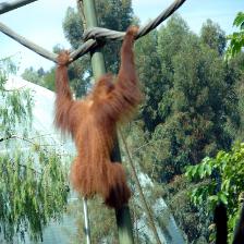
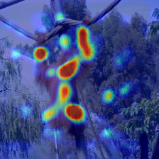
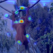
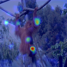
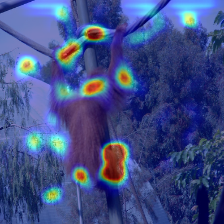
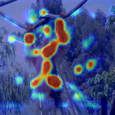
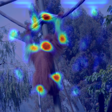
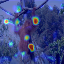
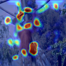
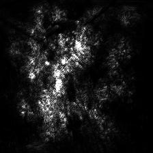
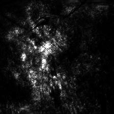
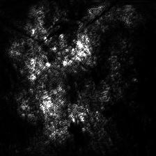
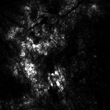
Input image CAM GradCAM++ IG Original example $\mathbf{x}$ Adversarial example $\mathbf{x}^{\prime}$ $I(\cdot,t)$ $I(\cdot,y^{\prime})$ correlation: 0.4782 correlation: 0.5039 $I(\cdot,t)$ $I(\cdot,y^{\prime})$ correlation: 0.5018 correlation: 0.5472 $I(\cdot,t)$ $I(\cdot,y^{\prime})$ correlation: 0.4040 correlation: 0.3911

Figure 1: Interpretation ($I$) of benign ($\mathbf{x}$) and adversarial ($\mathbf{x}^{\prime}$) image from Restricted ImageNet (Tsipras et al., 2019) with respect to the true label $y$=‘monkey’ and the target label $y^{\prime}$=‘fish’. Here the adversarial example is generated by 10-step PGD attack with perturbation size $0.02$ on Wide-Resnet (Madry et al., 2018), and we consider three types of interpretation maps, CAM, GradCAM++ and IG. Given an interpretation method, the first column is $I(\mathbf{x},y)$ versus $I(\mathbf{x}^{\prime},y)$, the second column is $I(\mathbf{x},y^{\prime})$ versus $I(\mathbf{x}^{\prime},y^{\prime})$, and all maps under each category are normalized w.r.t. their largest value. At the bottom of each column, we quantify the resulting interpretation discrepancy by Kendall’s Tau order rank correlation (Selvaraju et al., 2017) between every pair of $I(\mathbf{x},i)$ and $I(\mathbf{x}^{\prime},i)$ for $i=y$ or $y^{\prime}$.

PSM-type methods.

PSM assigns importance scores to individual pixels toward explaining the classification decision about an input. Examples of commonly-used approaches include vanilla gradient (Simonyan et al., 2013), guided backpropogation (Springenberg et al., 2014), SmoothGrad (Smilkov et al., 2017), and integrated gradient (IG) (Sundararajan et al., 2017). In particular, IG satisfies the completeness attribution axiom that PSM ought to obey. Specifically, it averages gradient saliency maps for interpolations between an input $\mathbf{x}$ and a baseline image $\mathbf{a}$:

$$[I_{\mathrm{IG}}(\mathbf{x},c)]_{i}=(x_{i}-a_{i})\int_{\alpha=0}^{1}\frac{\partial f_{c}(\mathbf{a}+\alpha(\mathbf{x}-\mathbf{a}))}{\partial x_{i}}d\alpha$$

$$\approx(x_{i}-a_{i})\sum_{j=1}^{m}\frac{\partial f_{c}(\mathbf{a}+\frac{j}{m}(\mathbf{x}-\mathbf{a}))}{\partial x_{i}}\frac{1}{m},~{}i\in[d],$$ (2)

where $m$ is the number of steps in the Riemman approximation of the integral. The completeness axiom (Sundararajan et al., 2017, Proposition 1) states that $\sum_{i=1}^{d}[I_{\mathrm{IG}}(\mathbf{x},c)]_{i}=f_{c}(\mathbf{x})-f_{c}(\mathbf{a})$, where the baseline image $\mathbf{a}$ is often chosen such that $f_{c}(\mathbf{a})\approx 0$, e.g., the black image. Note that CAM also satisfies the completeness axiom. PSM is able to highlight fine-grained details in the image, but is computationally intensive and not quite class-discriminative compared to CAM (Selvaraju et al., 2017).

Interpretation discrepancy caused by adversarial perturbations.

Let $\mathbf{x}^{\prime}=\mathbf{x}+\bm{\delta}$ represent an adversarial example w.r.t. $\mathbf{x}$, where $\bm{\delta}$ denotes an adversarial perturbation. By replacing the input image $\mathbf{x}$ with $\mathbf{x}^{\prime}$, a CNN will be fooled from the true label $y$ to the target (incorrect) label $y^{\prime}$. It was recently shown in (Xu et al., 2019b, a) that the adversary could introduce an evident interpretation discrepancy w.r.t. both the true and the target label in terms of $I(\mathbf{x},y)$ vs. $I(\mathbf{x}^{\prime},y)$, and $I(\mathbf{x},y^{\prime})$ vs. $I(\mathbf{x}^{\prime},y^{\prime})$. An illustrative example is provided in Figure 1. We see that an adversary suppresses the network interpretation w.r.t. the true label $y$ but promotes the interpretation w.r.t. the target label $y^{\prime}$. We also observe that compared to IG, CAM and GradCAM++ better localize class-specific discriminative regions.

The example in Figure 1 provides two implications on the robustness of classification versus interpretation discrepancy. First, an adversarial example designed for misclassification gives rise to interpretation discrepancy. Spurred by that, the problem of interpretability sneaking attack arises (Zhang et al., 2018; Subramanya et al., 2018): One may wonder whether or not it is easy to generate adversarial examples that mistake classification but keep interpretation intact. If such adversarial vulnerability exists, it could have serious consequences when classification and interpretation are jointly used in tasks like medical diagnosis  (Subramanya et al., 2018), and call into question the faithfulness of interpretation to network classification. It is also suggested from interpretation discrepancy that an interpreter itself could be quite sensitive to input perturbations (even if they were not designed for misclassification). Spurred by that, the robustness of interpretation provides a supplementary robustness metric for CNNs (Ghorbani et al., 2019; Dombrowski et al., 2019; Chen et al., 2019).

3 Robustness of Classification vs. Robustness of Interpretation

In this section, we revisit the validity of interpretability sneaking attack (ISA) from the perspective of interpretation discrepancy. We show that it is in fact quite challenging to force an adversarial example to mitigate its associated interpretation discrepancy. Further, we propose a novel measure of interpretation discrepancy, and theoretically show that constraining it prevents the success of adversarial attacks (for misclassification).

Previous work (Zhang et al., 2018; Subramanya et al., 2018) showed that it is not difficult to prevent adversarial examples from having large interpretation discrepancy when the latter is measured w.r.t. a single class label (either the true label $y$ or the target label $y^{\prime}$). However, we see from Figure 1 that the prediction-evasion adversarial attack alters interpretation maps w.r.t. both $y$ and $y^{\prime}$. This motivates us to rethink whether the single-class interpretation discrepancy measure is proper, and whether ISA is truly easy to bypass an interpretation discrepancy check.

We consider the generic form of $\ell_{p}$-norm based interpretation discrepancy,

$$\mathcal{D}\left(\mathbf{x},\mathbf{x}^{\prime}\right)=({1}/{|\mathcal{C}|})\sum_{i\in\mathcal{C}}\left\|I(\mathbf{x},i)-I(\mathbf{x}^{\prime},i)\right\|_{p},$$ (3)

where recall that $\mathbf{x}$ and $\mathbf{x}^{\prime}$ are natural and adversarial examples respectively, $I$ represents an interpreter, e.g., CAM or IG, $\mathcal{C}$ denotes the set of class labels used in $I$, $|\mathcal{C}|$ is the cardinality of $\mathcal{C}$, and we consider $p\in\{1,2\}$ in this paper. Clearly, a specification of (3) relies on the choice of $\mathcal{C}$ and $p$. The specification of (3) with $\mathcal{C}=\{y,y^{\prime}\}$ and $p=1$ leads to the $\ell_{1}$ 2-class interpretation discrepancy measure,

$$\mathcal{D}_{2,\ell_{1}}\left(\mathbf{x},\mathbf{x}^{\prime}\right)=(1/2) \left(\left\|I(\mathbf{x},y)-I(\mathbf{x}^{\prime},y)\right\|_{1}\right.$$

$$\left.+\left\|I(\mathbf{x},y^{\prime})-I(\mathbf{x}^{\prime},y^{\prime})\right\|_{1}\right).$$ (4)

Rationale behind (3).

Compared to the previous works (Zhang et al., 2018; Subramanya et al., 2018) which used a single class label, we choose $\mathcal{C}=\{y,y^{\prime}\}$, motivated by the fact that an interpretation discrepancy occurs w.r.t. both $y$ and $y^{\prime}$ (Figure 1). Moreover, although Euclidean distance (namely, $\ell_{2}$ norm or its square) is arguably one of the most commonly-used discrepancy metrics (Zhang et al., 2018), we show in Proposition 1 that the proposed interpretation discrepancy measure $\mathcal{D}_{2,\ell_{1}}\left(\mathbf{x},\mathbf{x}^{\prime}\right)$ has a perturbation-independent lower bound for any successful adversarial attack. This provides an explanation on why it could be difficult to mitigate the interpretation discrepancy caused by a successful attack. As will be evident later, the use of $\ell_{1}$ norm also outperforms the $\ell_{2}$ norm in evaluation of interpretation discrepancy.

Proposition 1.

Given a classifier $f(\mathbf{x})\in\mathbb{R}^{C}$ and its interpreter $I(\mathbf{x},c)$ for $c\in[C]$, suppose that the interpreter satisfies the completeness axiom, namely, $\sum_{i}[I(\mathbf{x},c)]_{i}=f_{c}(\mathbf{x})$ for a possible scaling factor $a$. For a natural example $\mathbf{x}$ and an adversarial example $\mathbf{x}^{\prime}$ with prediction $y$ and $y^{\prime}$ ($\neq y$) respectively, $\mathcal{D}_{2,\ell_{1}}\left(\mathbf{x},\mathbf{x}^{\prime}\right)$ in (3) has the perturbation-independent lower bound,

$$\mathcal{D}_{2,\ell_{1}}\left(\mathbf{x},\mathbf{x}^{\prime}\right)\geq(1/2)\left(f_{y}(\mathbf{x})-f_{y^{\prime}}(\mathbf{x})\right).$$ (5)

Proof: See proof and a generalization in Appendix A. $\square$

Proposition 1 connects $\mathcal{D}_{2,\ell_{1}}\left(\mathbf{x},\mathbf{x}^{\prime}\right)$ with the classification margin $f_{y}(\mathbf{x})-f_{y^{\prime}}(\mathbf{x})$. Thus, if a classifier has a large classification margin on the natural example $\mathbf{x}$, it will be difficult to find a successful adversarial attack with small interpretation discrepancy. In other words, constraining the interpretation discrepancy prevents misclassification of a perturbed input since making its attack successful becomes infeasible under $\mathcal{D}_{2,\ell_{1}}\left(\mathbf{x},\mathbf{x}^{\prime}\right)<\frac{1}{2}\left(f_{y}(\mathbf{x})-f_{y^{\prime}}(\mathbf{x})\right)$. Also, the completeness condition of $I$ suggests specifying (3) with CAM (1) or IG (2). Indeed, the robust attribution regularization proposed in (Chen et al., 2019) adopted IG. In this paper, we focus on CAM due to its light computation. In Appendix  A, we further extend Proposition 1 to interpreters satisfying a more general completeness axiom of the form $\sum_{i}[I(\mathbf{x},c)]_{i}=g(f_{c}(\mathbf{x}))$, where $g$ is a monotonically increasing function. In Appendix E, we demonstrate the empirical tightness of (5).

Attempt in generating ISA with minimum $\ell_{1}$ $2$-class interpretation discrepancy.

Next, we examine how the robustness of classification is coupled with the robustness of interpretation through the lens of ISA. We pose the following optimization problem for design of ISA, which not only fools a classifier’s decision but also minimizes the resulting interpretation discrepancy,

$$\begin{array}[]{cl}\displaystyle\operatorname*{\text{minimize}}_{\bm{\delta}}&\lambda\max\{\max_{j\neq y^{\prime}}f_{j}(\mathbf{x}+\bm{\delta})-f_{y^{\prime}}(\mathbf{x}+\bm{\delta}),-\tau\}\\ &+\mathcal{D}_{2,\ell_{1}}\left(\mathbf{x},\mathbf{x}+\bm{\delta}\right)\\ \operatorname*{\text{subject to}}&\|\bm{\delta}\|_{\infty}\leq\epsilon.\end{array}$$ (9)

In (9), the first term corresponds to a C&W-type attack loss (Carlini & Wagner, 2017), which reaches $-\tau$ if the attack succeeds in misclassification, $\tau>0$ (e.g., $0.1$ used in the paper) is a tolerance on the classification margin of a successful attack between the target label $y^{\prime}$ and the non-target top-1 prediction label, $\mathcal{D}_{2,\ell_{1}}$ was defined by (3), $\lambda>0$ is a regularization parameter that strikes a balance between the success of an attack and its resulting interpretation discrepancy, and $\epsilon>0$ is a (pixel-level) perturbation size.

To approach ISA (9) with minimum interpretation discrepancy, we perform a bisection on $\lambda$ until there exists no successful attack that can be found when $\lambda$ further decreases. We call an attack a successful ISA if the value of the attack loss stays at $-\tau$ (namely, a valid adversarial example) and the minimum $\lambda$ is achieved (namely, the largest penalization on interpretation discrepancy). We solve problem (9) by projected gradient descent (PGD), with sub-gradients taken at non-differentiable points. We consider only targeted attacks to better evaluate the effect on interpretability of target classes, although this approach can be extended to an untargeted setting (e.g., by target label-free interpretation discrepancy measure introduced in the next section).

Successful ISA is accompanied by non-trivial $\ell_{1}$ 2-class interpretation discrepancy.

We then empirically justify that how the choice of interpretation discrepancy measure plays a crucial role on drawing the relationship between robustness of classification and robustness of interpretation. We generate successful ISAs by solving problem (9) under different values of the perturbation size $\epsilon$ and different specifications of the interpretation discrepancy measure (3), including $\ell_{1}$/$\ell_{2}$ 1-class (true class $y$), $\ell_{2}$ 2-class, and $\ell_{1}$/$\ell_{2}$ all-class measure. In Figure 2-(a) and (b), we present the interpretation discrepancy induced by successful ISAs versus the perturbation strength $\epsilon$. One may expect that a stronger ISA (with larger $\epsilon$) could more easily suppress the interpretation discrepancy. However, we observe that compared to $\ell_{1}$/$\ell_{2}$ 1-class, $\ell_{2}$ 2-class, and $\ell_{1}$/$\ell_{2}$ all-class cases, it is quite difficult to mitigate the $\ell_{1}$ 2-class interpretation discrepancy (3) even as the attack power goes up. This is verified by a) its high interpretation discrepancy score and b) its flat slope of discrepancy score against $\epsilon$.

Furthermore, Figure 2-(c) shows CAMs of adversarial examples w.r.t. the true label $y$ and the target label $y^{\prime}$ generated by $\ell_{1}$ 1/2/all-class ISAs. We observe that the 1-class measure could give a false sense of ease of preventing adversarial perturbations from interpretation discrepancy. Specifically, although the interpretation discrepancy w.r.t. $y$ of the $\ell_{1}$ 1-class ISA is minimized, the discrepancy w.r.t. $y^{\prime}$ remains large, supported by the observation that the resulting correlation between $I(\mathbf{x}^{\prime},y^{\prime})$ and $I(\mathbf{x},y^{\prime})$ is even smaller than that of PGD attack; see the $4$th column of Figure 2-(c). Thus, the vulnerability of an image classifier (against adversarial perturbations) is accompanied by interpretation discrepancy only if the latter is properly measured. We refer readers to Appendix B for more comprehensive experimental results on the evaluation of interpretation discrepancy through the lens of ISA.

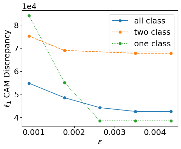
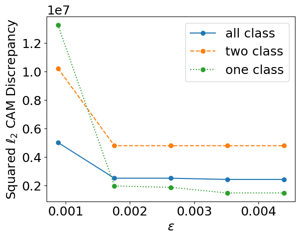
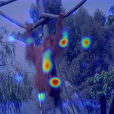
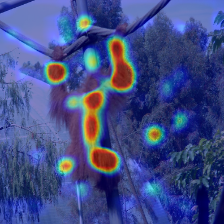
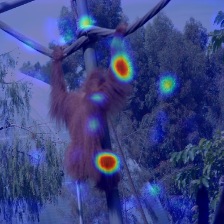
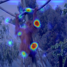
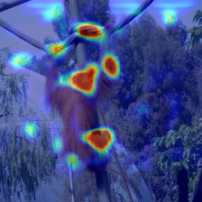
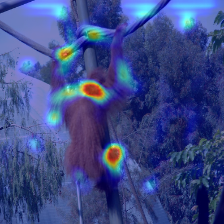
(a)	(b)
	$I(\cdot,t)$ $I(\cdot,y^{\prime})$ original image $\mathbf{x}$ 10-step PGD attack $\mathbf{x}^{\prime}$ $\ell_{1}$ 2-class ISA $\mathbf{x}^{\prime}$ $\ell_{1}$ 1-class ISA $\mathbf{x}^{\prime}$ $\ell_{1}$ all-class ISA $\mathbf{x}^{\prime}$ correlation: 0.4782 correlation: 0.5213 correlation: 0.7107 correlation: 0.5342 correlation: 0.5039 correlation: 0.5416 correlation: 0.4129 correlation: 0.5561
	(c)

Figure 2: Interpretation discrepancy induced by successful ISAs. Here the same image as Figure 1 is considered. (a) ISAs using CAM-based $\ell_{1}$ 1/2/all-class discrepancy measure versus perturbation size $\epsilon$, (b) ISAs using CAM-based $\ell_{2}$ 1/2/all-class discrepancy measure versus $\epsilon$, (c) CAM interpretation of example in Figure 1 and its adversarial counterparts from PGD attack and ISAs. All interpretation maps are normalized w.r.t. the common largest value. At the bottom of each interpretation map $I(\mathbf{x}^{\prime},\cdot)$, we quantify the interpretation discrepancy by Kendall’s Tau order rank correlation between $I(\mathbf{x}^{\prime},i)$ and $I(\mathbf{x},i)$ for $i\in\{y,y^{\prime}\}$, where $\mathbf{x}^{\prime}$ is obtained from PGD attack or each specification of ISA.

4 Interpretability-Aware Robust Training

We recall from Sec. 3 that adversarial examples that intend to fool a classifier could find it difficult to evade the $\ell_{1}$ 2-class interpretation discrepancy. Thus, constraining the interpretation discrepancy helps to prevent misclassification. Spurred by that, we introduce an interpretability based defense method that penalizes interpretation discrepancy to achieve high classification robustness.

Target label-free interpretation discrepancy.

Different from attack generation, the $\ell_{1}$ 2-class discrepancy measure (3) cannot directly be used by a defender since the target label $y^{\prime}$ specified by the adversary is not known a priori. To circumvent this issue, we propose to approximate the interpretation discrepancy w.r.t. the target label by weighting discrepancies from all non-true classes according to their importance in prediction. This modifies (3) to

$$\tilde{\mathcal{D}}\left(\mathbf{x},\mathbf{x}^{\prime}\right)= (1/2)\left\|I(\mathbf{x},y)-I(\mathbf{x}^{\prime},y)\right\|_{1}$$

$$+(1/2)\sum_{i\neq t}\frac{e^{f(\mathbf{x}^{\prime})_{i}}}{\sum_{i^{\prime}}e^{f(\mathbf{x}^{\prime})_{i^{\prime}}}}||I(\mathbf{x},i)-I(\mathbf{x}^{\prime},i)||_{1},$$ (10)

where the softmax function $\frac{e^{f(\mathbf{x}^{\prime})_{i}}}{\sum_{i}e^{f(\mathbf{x}^{\prime})_{i}}}$ adjusts the importance of non-true labels according to their classification confidence. Clearly, when $\mathbf{x}^{\prime}$ succeeds in misclassification, the top-1 predicted class of $\mathbf{x}^{\prime}$ becomes the target label and the resulting interpretation discrepancy is most penalized.

Interpretability-aware robust training.

We propose to train a classifier against the worst-case interpretation discrepancy (4), yielding the min-max optimization problem

$$\displaystyle\operatorname*{\text{minimize}}_{\bm{\theta}}~{}\mathbb{E}_{(\mathbf{x},t)\sim\mathcal{D}_{\mathrm{train}}}\left[f_{\mathrm{train}}(\bm{\theta};\mathbf{x},y)+\gamma\tilde{D}_{\mathrm{worst}}(\mathbf{x},\mathbf{x}^{\prime})\right],$$ (11)

where $\bm{\theta}$ denotes the model parameters to be learnt. In (11), $\mathcal{D}_{\mathrm{train}}$ denotes the training dataset, $f_{\mathrm{train}}$ is the training loss (e.g., cross-entropy loss), $\tilde{D}_{\mathrm{worst}}(\mathbf{x},\mathbf{x}^{\prime})$ denotes a measure of the worst-case interpretation discrepancy between the benign and the perturbed inputs $\mathbf{x}$ and $\mathbf{x}^{\prime}$, and the regularization parameter $\gamma>0$ controls the tradeoff between clean accuracy and robustness of network interpretability. Note that the commonly-used adversarial training method (Madry et al., 2018) adopts the adversarial loss $\operatorname*{\text{maximize}}_{\|\bm{\delta}\|_{\infty}\leq\epsilon}f_{\mathrm{train}}(\bm{\theta},\mathbf{x}+\bm{\delta};\mathbf{x},y)$ rather than the standard training loss in (11). Our experiments will show that the promotion of robust interpretation via (11) is able to achieve robustness in classification.

Next, we introduce two types of worst-case interpretation discrepancy measure based on our different views on input perturbations. That is,

$$\tilde{D}_{\mathrm{worst}}(\mathbf{x},\mathbf{x}^{\prime})\mathrel{\mathop{:}}=\operatorname*{\text{maximize}}_{\|\bm{\delta}\|_{\infty}\leq\epsilon}\tilde{\mathcal{D}}\left(\mathbf{x},\mathbf{x}+\bm{\delta}\right),$$ (12)

$$\tilde{D}_{\mathrm{worst}}(\mathbf{x},\mathbf{x}^{\prime})\mathrel{\mathop{:}}=\tilde{\mathcal{D}}\left(\mathbf{x},\mathbf{x}+\operatorname*{arg\,max}_{\|\bm{\delta}\|_{\infty}\leq\epsilon}\,[f_{\mathrm{train}}(\bm{\theta};\mathbf{x}+\bm{\delta},y)]\right),$$ (13)

where $\tilde{\mathcal{D}}$ was defined in (4). In (12) and (13), the input perturbation $\bm{\delta}$ represents the adversary shooting for misinterpretation and misclassification, respectively. For ease of presentation, we call the proposed interpretability-aware robust training methods Int and Int2 by using (12) and (13) in (11) respectively. We will empirically show that both Int and Int2 can achieve robustness in classification and interpretation simultaneously. It is also worth noting that Int2 training is conducted by alternative optimization: The inner maximization step w.r.t. $\bm{\delta}$ generates adversarial example $\mathbf{x}^{\prime}$ for misclassification, and then forms $\tilde{D}_{\mathrm{worst}}(\mathbf{x},\mathbf{x}^{\prime})$; The outer minimization step minimizes the regularized standard training loss w.r.t. $\bm{\theta}$ by fixing $\mathbf{x}^{\prime}$, ignoring the dependence of $\mathbf{x}^{\prime}$ on $\bm{\theta}$.

Difference from (Chen et al., 2019).

The recent work (Chen et al., 2019) proposed improving adversarial robustness by leveraging robust IG attributions. However, different from (Chen et al., 2019), our approach is motivated by the importance of the $\ell_{1}$ 2-class interpretation discrepancy measure. We will show in Sec. 5 that the incorporation of interpretation discrepancy w.r.t. target class labels, namely, the second term in (4), plays an important role in boosting classification and interpretation robustness. We will also show that our proposed method is sufficient to improve adversarial robustness even in the absence of adversarial loss. This implies that robust interpretations alone helps robust classification when interpretation maps are measured with a proper metric. Furthermore, we find that the robust attribution regularization method (Chen et al., 2019) becomes less effective when the attack becomes stronger. Last but not least, beyond IG, our proposed theory and method apply to any network interpretation method with the completeness axiom.

5 Experiments

In this section, we demonstrate the effectiveness of our proposed methods in $5$ aspects: a) classification robustness against PGD attacks (Madry et al., 2018; Athalye et al., 2018), b) defending against unforeseen adversarial attacks (Kang et al., 2019), c) computation efficiency, d) interpretation robustness when facing attacks against interpretability (Ghorbani et al., 2019), and e) visualization of perceptually-aligned robust features (Engstrom et al., 2019). Our codes are available at https://github.com/AkhilanB/Proper-Interpretability

Datasets and CNN models.

We evaluate networks trained on the MNIST and CIFAR-10 datasets, and a Restricted ImageNet (R-ImageNet) dataset used in (Tsipras et al., 2019). We consider three models, Small (for MNIST and CIFAR), Pool (for MNIST) and WResnet (for CIFAR and R-ImageNet). Small is a small CNN architecture consisting of three convolutional layers of 16, 32 and 100 filters. Pool is a CNN architecture with two convolutional layers of 32 and 64 filters each followed by max-pooling which is adapted from (Madry et al., 2018). WResnet is a Wide Resnet from (Zagoruyko & Komodakis, 2016) .

Attack models.

First, to evaluate robustness of classification, we consider conventional PGD attacks with different steps and perturbation sizes (Madry et al., 2018; Athalye et al., 2018) and unforeseen adversarial attacks (Kang et al., 2019) that are not used in robust training. Second, to evaluate the robustness of interpretation, we consider attacks against interpretability (AAI) (Ghorbani et al., 2019; Dombrowski et al., 2019), which produce input perturbations to maximize the interpretation discrepancy rather than misclassification. We refer readers to Appendix C for details on the generation of AAI. Furthermore, we consider ISA (9) under different discrepancy measures to support our findings in Figure 2. Details are presented in Appendix B.

Training methods.

We consider $6$ baselines: i) standard training (Normal), ii) adversarial training (Adv) (Madry et al., 2018), iii) TRADES (Zhang et al., 2019), iv) IG-Norm that uses IG-based robust attribution regularization (Chen et al., 2019), v) IG-Sum-Norm (namely, IG-Norm with adversarial loss), and vi) Int using $\ell_{1}$ $1$-class discrepancy (Int-one-class). Additionally, we consider $4$ variants of our method: i) Int, namely, (11) plus (12), ii) Int with adversarial loss (Int-Adv), iii) Int2, namely,(11) plus (13), and iv) Int2 with adversarial loss (Int2-Adv).

Unless specified otherwise, we choose the perturbation size $\epsilon=0.3$ on MNIST, $8/255$ on CIFAR and $0.003$ for R-ImageNet for robust training under an $\ell_{\infty}$ perturbation norm. We refer readers to Appendix D for more details. Also, we set the regularization parameter $\gamma$ as $0.01$ in (11); see a justification in Appendix F. Note that when training WResnet, the IG-based robust training methods (IG-Norm and IG-Norm-Sum) are excluded due to the prohibitive computation cost of computing IG. For our main experiments, we focus on the Small and WResnet architectures, but additional results on the Pool architecture are included in Appendix H.

5.1 Classification against prediction-evasion attacks

Robustness & training efficiency.

In Figure 3, we present the training time (left $y$-axis) and the adversarial test accuracy (right $y$-axis) for different training methods ($x$-axis) that are ranked in a decreasing order of computation complexity. Training times are evaluated on a 2.60 GHz Intel Xeon CPU. Here adversarial test accuracy (ATA) is found by performing $200$-step $\ell_{\infty}$-PGD attacks of perturbation size $\epsilon=0.3$ and $0.4$ on the learned MNIST model Small over $200$ random test set points. Note that all methods that use adversarial losses (IG-Norm-Sum, Int-Adv, Int2-Adv, TRADES and Adv) can yield robust classification at $\epsilon=0.3$ (with ATA around $80\%$). However, among interpretability-regularized defense methods (IG-Norm, Int-one-class, Int, Int2), only the proposed Int and Int2 methods provide competitive ATAs. As the PGD attack becomes stronger ($\epsilon=0.4$), Int and Int2 based methods outperform all others in ATA. This implies the benefit of robust interpretation when facing stronger prediction-evasion attacks; see more details in later results.

In Figure 3, we also find that both IG-Norm (Chen et al., 2019) and Int-one-class are insufficient to provide satisfactory ATA. The verifies the importance on penalizing the 2-class interpretation discrepancy to render robust classification. We further observe that IG-based methods make training time (per epoch) significantly higher, e.g., $\geq 4$ times more than Int.

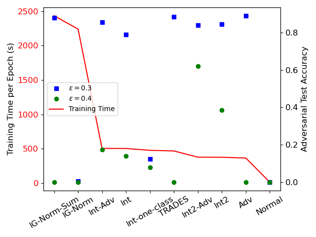
Figure 3: Computation time per epoch and adversarial test accuracy for a Small MNIST model trained with different methods.

Robustness against PGD attacks with different steps and perturbation sizes.

It was shown in (Athalye et al., 2018; Carlini, 2019) that some defense methods cause obfuscated gradients, which give a false sense of security. There exist two characteristic behaviors of obfuscated gradients: (a) Increasing perturbation size does not increase attack success; (b) One-step attacks perform better than iterative attacks. Motivated by that, we evaluate our interpretability-aware robust training methods under PGD attacks with different perturbation sizes and steps.

Table 1 reports ATA of interpretability-aware robust training compared to various baselines over MNIST and CIFAR, where $200$-step PGD attacks are conducted for robustness evaluation under different values of perturbation size $\epsilon$. As we can see, ATA decreases as $\epsilon$ increases, violating the behavior (a) of obfuscated gradients. We also observe that compared to Adv and TRADES, Int and Int2 achieve slightly worse standard accuracy ($\epsilon=0$) and ATA on $\epsilon$ less than the value used for training. However, when the $\epsilon$ used in the PGD attack achieves the value used for robust training, Int and Int2 achieve better ATA than Adv on CIFAR-10 ($0.270$ and $0.290$ vs $0.170$). Interestingly, the advantage of Int and Int2 becomes more evident as the adversary becomes stronger, i.e., $\epsilon>0.3$ on MNIST and $\epsilon>8/255$ on CIFAR-10. We highlight that such a robust classification is achieved by promoting robustness of interpretations alone (without using adversarial loss).

It is worth mentioning that IG-Norm fails to defend PGD attack with $\epsilon=0.3$ for the MNIST model Small. We further note that Int-one-class performs much worse than Int, supporting the importance of using a 2-class discrepancy measure. As will be evident later, IG-Norm is also not the best to render robustness in interpretation (Table 3). In Table A3 of Appendix G, we further show that as the number of iterations of PGD attacks increases, the ATA of our proposed defensive schemes decreases accordingly. This violates the typical behavior (b) of obfuscated gradients.

Method $\epsilon=0$ 0.05 0.1 0.2 0.3 0.35 0.4 MNIST, Small Normal 1.000 0.530 0.045 0.000 0.000 0.000 0.000 Adv 0.980 0.960 0.940 0.925 0.890 0.010 0.000 TRADES 0.970 0.970 0.955 0.930 0.885 0.000 0.000 IG-Norm 0.985 0.950 0.895 0.410 0.005 0.000 0.000 IG-Norm-Sum 0.975 0.955 0.935 0.910 0.880 0.115 0.000 Int-one-class 0.975 0.635 0.330 0.140 0.125 0.115 0.080 Int 0.950 0.930 0.905 0.840 0.790 0.180 0.140 Int-Adv 0.935 0.945 0.905 0.880 0.855 0.355 0.175 Int2 0.950 0.945 0.935 0.890 0.845 0.555 0.385 Int2-Adv 0.955 0.925 0.915 0.880 0.840 0.655 0.620 $\epsilon=0$ 2/255 4/255 6/255 8/255 9/255 10/255 CIFAR-10, WResnet Normal 0.765 0.250 0.070 0.060 0.060 0.060 0.060 Adv 0.720 0.605 0.485 0.330 0.170 0.145 0.085 TRADES 0.765 0.610 0.460 0.295 0.170 0.140 0.100 Int-one-class 0.685 0.505 0.360 0.190 0.065 0.040 0.025 Int 0.735 0.630 0.485 0.365 0.270 0.240 0.210 Int-Adv 0.665 0.585 0.510 0.385 0.320 0.300 0.280 Int2 0.690 0.595 0.465 0.360 0.290 0.245 0.220 Int2-Adv 0.680 0.585 0.485 0.405 0.335 0.310 0.285 R-ImageNet, WResnet Normal 0.770 0.070 0.035 0.030 0.040 0.030 0.030 Adv 0.790 0.455 0.230 0.100 0.070 0.060 0.050 Int 0.660 0.570 0.460 0.385 0.280 0.250 0.220 Int2 0.655 0.545 0.480 0.355 0.265 0.205 0.170

Table 1: Evaluation of 200-step PGD accuracy under different perturbation sizes $\epsilon$. ATA with $\epsilon=0$ reduces to standard test accuracy.

Method Gabor Snow JPEG $\ell_{\infty}$ JPEG $\ell_{2}$ JPEG $\ell_{1}$ CIFAR-10, Small Normal 0.125 0.000 0.000 0.030 0.000 Adv 0.190 0.115 0.460 0.380 0.230 TRADES 0.220 0.085 0.425 0.300 0.070 IG-Norm 0.155 0.015 0.000 0.000 0.000 IG-Norm-Sum 0.185 0.110 0.480 0.375 0.215 Int 0.160 0.105 0.440 0.345 0.260 Int-Adv 0.150 0.120 0.340 0.310 0.235 Int2 0.130 0.115 0.440 0.365 0.295 Int2-Adv 0.110 0.135 0.360 0.315 0.260

Table 2: ATA on different unforeseen attacks in (Kang et al., 2019). Best results in each column are highlighted.

Robustness against unforeseen attacks.

In Table 2, we present ATA of interpretability-aware robust training and various baselines for defending attacks (Gabor, Snow, JPEG $\ell_{\infty}$, JPEG $\ell_{2}$, and JPEG $\ell_{1}$) recently proposed in (Kang et al., 2019). These attacks are called ‘unforeseen attacks’ since they are not met by PGD-based robust training and often induce larger perturbations than conventional PGD attacks. We use the same attack parameters as used in (Kang et al., 2019) over 200 random test points. To compare with IG-based methods, we present results on the Small architecture since computing IG on the WResnet architecture is computationally costly. As we can see, Int and Int2 significantly outperform IG-Norm especially under Snow and JPEG $\ell_{p}$ attacks. Int and Int2 also yield competitive robustness compared to the robust training methods that use the adversarial training loss (Adv, TRADES, IG-Norm-Sum, Int-Adv, Int2-Adv).

5.2 Robustness of interpretation against AAI

Recall that attack against interpretability (AAI) attempts to generate an adversarial interpretation map (namely, CAM in experiments) that is far away from the benign CAM of the original example w.r.t. the true label; see details in Appendix C. The performance of AAI is then measured by the Kendall’s Tau order rank correlation between the adversarial and the benign interpretation maps (Chen et al., 2019). The higher the correlation is, the more robust the model is in interpretation. Reported rank correlations are averaged over 200 random test set points.

In Table 3, we present the performance of obtained robust models against AAI with different attack strengths (in terms of the input perturbation size $\epsilon$); see Table A7 of Appendix H for results on additional dataset and networks. The insights learned from Table 3 are summarized as below. First, the normally trained model (Normal) does not automatically offer robust interpretation, e.g., against AAI with $\epsilon\geq 0.2$ in MNIST. Second, the interpretation robustness of networks learned using adversarial training methods Adv and TRADES is worse than that learnt from interpretability-regularized training methods (except IG-Norm) as the perturbation size $\epsilon$ increases ($\epsilon\geq 0.3$ for MNIST and $\epsilon\geq 8/255$ for R-ImageNet). Third, when the adversarial training loss is not used, our proposed methods Int and Int2 are consistently more robust than IG-Norm, and their advantage becomes more evident as $\epsilon$ increases in MNIST.

Method	$\epsilon=0.05$	0.1	0.2	0.3	0.35	0.4
MNIST, Small
Normal	0.907	0.797	0.366	-0.085	-0.085	-0.085
Adv	0.978	0.955	0.910	0.857	0.467	0.136
TRADES	0.978	0.955	0.905	0.847	0.450	0.115
IG-Norm	0.958	0.894	0.662	0.278	0.098	0.094
IG-Norm-Sum	0.976	0.951	0.901	0.850	0.659	0.389
Int-one-class	0.874	0.818	0.754	0.692	0.461	0.278
Int	0.982	0.968	0.941	0.913	0.504	0.320
Int-Adv	0.980	0.965	0.936	0.912	0.527	0.348
Int2	0.982	0.967	0.941	0.918	0.612	0.351
Int2-Adv	0.982	0.971	0.950	0.931	0.709	0.503
	$\epsilon=2/255$	4/255	6/255	8/255	9/255	10/255
R-ImageNet, WResnet
Normal	0.851	0.761	0.705	0.673	0.659	0.619
Adv	0.975	0.947	0.916	0.884	0.870	0.858
Int	0.988	0.974	0.960	0.946	0.939	0.932
Int2	0.989	0.977	0.965	0.952	0.946	0.939

Table 3: Performance of AAI for different values of perturbation size $\epsilon$ in terms of Kendall’s Tau order rank correlation between the original and adversarial interpretation maps. High interpretation robustness corresponds to large correlation value.

5.3 Perceptually-aligned robust features

In Figure 4, we visually examine whether or not our proposed interpretability-aware training methods (Int and Int2) are able to render perceptually-aligned robust features similar to those found by (Engstrom et al., 2019) using Adv. Figure 4 shows that similar texture-aligned robust features can be acquired from networks trained using Int and Int2 regardless of the choice of input seed image. This observation is consistent with features learnt from Adv. By contrast, the networks trained using Normal and IG-Norm fail to yield robust features; see results learnt from IG-Norm under CIFAR-10 Small model in Appendix I.

Seed Images Normal Adv Int Int2

Figure 4: Feature visualization at neuron $3$ under CIFAR-10 WResnet model trained by different methods. Column $1$ contains different seed images to maximize neuron’s activation. Columns $2$-$5$ contain generated features w.r.t. each seed image.

6 Conclusion

In this paper, we investigate the connection between network interpretability and adversarial robustness. We show theoretically and empirically that with the correct choice of discrepancy measure, it is difficult to hide adversarial examples from interpretation. We leverage this discrepancy measure to develop a interpretability-aware robust training method that displays 1) high classification robustness in a variety of settings and 2) high robustness of interpretation. Future work will extend our proposal to a semi-supervised setting by incorporating unlabeled training data.

Appendix

Appendix A Proof of Proposition 1

We first prove a generalization of Proposition 1 assuming a more general completeness axiom: $\forall c\in[C],$ suppose $g(f_{c}(\mathbf{x}))=\sum_{i}[I(\mathbf{x},c)]_{i}$ where $g$ is a monotonically increasing function, e.g., a positive scaling function. The standard completeness axiom (Sundararajan et al., 2017) uses the identity function for $g$: $g(z)=z$.

Using the generalized completeness axiom, we obtain that

$$g(f_{y^{\prime}}(\mathbf{x}^{\prime}))-g(f_{y^{\prime}}(\mathbf{x}))= \sum_{i}([I(\mathbf{x}^{\prime},y^{\prime})]_{i}-[I(\mathbf{x},y^{\prime})]_{i})$$

$$\leq \sum_{i}\left|[I(\mathbf{x}^{\prime},y^{\prime})]_{i}-[I(\mathbf{x},y^{\prime})]_{i}\right|=\|I(\mathbf{x}^{\prime},y^{\prime})-I(\mathbf{x},y^{\prime})\|_{1}.$$ (14)

Similarly, we have

$$g(f_{y}(\mathbf{x}))-g(f_{y}(\mathbf{x}^{\prime}))\leq\|I(\mathbf{x},y)-I(\mathbf{x}^{\prime},y)\|_{1}.$$ (15)

Adding (14) and (15) rearranging yields

$$[g(f_{y^{\prime}}(\mathbf{x}^{\prime}))-g(f_{y}(\mathbf{x}^{\prime}))]+[g(f_{y}(\mathbf{x}))-g(f_{y^{\prime}}(\mathbf{x}))]\leq\|I(\mathbf{x}^{\prime},y^{\prime})-I(\mathbf{x},y)\|_{1}+\|I(\mathbf{x},y)-I(\mathbf{x}^{\prime},y)\|_{1}.$$ (16)

Since $f_{y^{\prime}}(\mathbf{x}^{\prime})-f_{y}(\mathbf{x}^{\prime})\geq 0$ and $g$ is monotonically increasing, $g(f_{y^{\prime}}(\mathbf{x}^{\prime}))-g(f_{y}(\mathbf{x}^{\prime}))\geq 0$. We then have $\|I(\mathbf{x}^{\prime},y^{\prime})-I(\mathbf{x},y^{\prime})\|_{1}+\|I(\mathbf{x},y)-I(\mathbf{x}^{\prime},y)\|_{1}\geq g(f_{y}(\mathbf{x}))-g(f_{y^{\prime}}(\mathbf{x}))$, which implies:

$$\mathcal{D}_{2,\ell_{1}}(\mathbf{x},\mathbf{x}^{\prime})\geq(1/2)[g(f_{y}(\mathbf{x}))-g(f_{y^{\prime}}(\mathbf{x}))].$$ (17)

This is a generalization of the bound in Proposition 1. Taking $g(z)=z$ yields Equation (5).

Appendix B Interpretability Sneaking Attack (ISA): Evaluation and Results

In what follows, we provide additional experiment results on examining the relationship between classification robustness and interpretation robustness through the lens of ISA. We evaluate the effect of interpretation discrepancy measure on ease of finding ISAs. Spurred by Figure 2, such an effect is quantified by calculating minimum discrepancy required in generating ISAs against different values of perturbation size $\epsilon$ in (9). We conduct experiments over $4$ network interpretation methods: i) CAM, ii) GradCAM++, iii) IG, and iv) internal representation at the penultimate (pre-softmax) layer (denoted by Repr).

In order to fairly compare among different interpretation methods, we compute a normalized discrepancy score (NDS) extended from (3): $\mathcal{D}_{\mathrm{norm}}=\frac{1}{|\mathcal{C}|}\sum_{i\in\mathcal{C}}\left\|\frac{I(\mathbf{x},i)-I(\mathbf{x}^{\prime},i)}{\max_{{j}}I(\mathbf{x},i)_{{j}}-\min_{{j}}I(\mathbf{x},i)_{{j}}}\right\|_{p}$. A larger value of NDS implies the more difficulty for ISA to alleviate interpretation discrepancy from adversarial perturbations. To quantify the strength of ISA against the perturbation size $\epsilon$, we compute an additional quantity called normalized slope (NSL) that measures the relative change of NDS for $\epsilon\in[\check{\epsilon},\hat{\epsilon}]$: $\mathcal{S}_{\mathrm{norm}}=\frac{|\mathcal{D}_{\mathrm{norm}}^{(\hat{\epsilon})}-\mathcal{D}_{\mathrm{norm}}^{(\check{\epsilon})}|/\mathcal{D}_{\mathrm{norm}}^{(\check{\epsilon})}}{(\hat{\epsilon}-\check{\epsilon})/\check{\epsilon}}$. The smaller NSL is, the more difficult it is for ISA to resist network interpretation changes as $\epsilon$ increases. In our experiment, we choose $\check{\epsilon}=\epsilon^{*}$ and $\hat{\epsilon}=1.6\,\epsilon^{*}$, where $\epsilon^{*}$ is the minimum perturbation size required for a successful PGD attack. Here we perform binary search over $\epsilon$ to find its smallest value for misclassification. Reported NDS and NSL statistics are averaged over a test set.

In Table A1, we present NDS and NSL of ISAs generated under different realizations of interpretation discrepancy measure (3), each of which is given by a combination of interpretation method (CAM, GradCAM++, IG or Repr), $\ell_{p}$ norm ($p\in\{1,2\}$) and number of interpreted classes. Note that Repr is independent of the number of classes, and thus we report NDS and NSL corresponding to Repr in the 2-class column of Table A1. Given an $\ell_{p}$ norm and an interpretation method, we consistently find that the use of 2-class measure achieves the largest NDS and smallest NSL at the same time. This implies that the 2-class discrepancy measure increases the difficulty for ISA to evade a network interpretability check. Moreover, given a class number and an interpretation method, we see that NDS under $\ell_{1}$ norm is greater than that under $\ell_{2}$ norm, since the former is naturally an upper bound of the latter. Also, the use of $\ell_{1}$ norm often yields a smaller value of NSL, implying that the $\ell_{1}$-norm based discrepancy measure is more resistant to ISA. Furthermore, by fixing the combination of $\ell_{1}$ norm and $2$ classes, we observe that IG is the most resistant to ISA due to its relatively high NDS and low ISA, and Repr yields the worst performance. However, compared to CAM, the computation cost of IG increases dramatically as the input dimension, the model size, and the number of steps in Riemman approximation increase. We find that it becomes infeasible to generate ISA using IG for WResnet under R-ImageNet within 200 hours.

Dataset Interpretation method $\ell_{1}$ norm $\ell_{2}$ norm 1-class 2-class all-class 1-class 2-class all-class MNIST CAM 3.0723/0.0810 3.2672/0.0223 2.5289/0.0414 0.3061/0.1505 0.5654/0.0321 0.4320/0.0459 GradCAM++ 3.1264/0.0814 3.1867/0.0221 2.5394/0.0366 0.3308/0.1447 0.5531/0.0289 0.4392/0.0456 IG 6.3604/0.0330 6.7884/0.0233 4.3667/0.2314 0.4476/0.0082 0.5766/0.0064 0.2160/0.0337 Repr n/a 2.3668/0.0404 n/a n/a 0.4129/0.0429 n/a CIFAR-10 CAM 1.9523/0.1450 2.5020/0.0496 1.7898/0.0774 0.1313/0.2369 0.3613/0.0668 0.2746/0.0809 GradCAM++ 1.9355/0.1439 2.4788/0.0513 1.8020/0.0745 0.1375/0.2346 0.3577/0.0676 0.2758/0.0769 IG 4.9499/0.0188 4.9794/0.0177 2.8541/0.1356 0.1230/0.0110 0.1309/0.0092 0.0878/0.0235 Repr n/a 1.7049/0.0785 n/a n/a 0.1288/0.0056 n/a R-ImageNet CAM 49.286/0.1005 61.975/0.0331 49.877/0.0557 1.9373/0.1526 2.6036/0.0791 2.0935/0.0863 GradCAM++ 39.761/0.1028 50.303/0.0453 42.390/0.0552 1.9185/0.1609 2.5869/0.0891 2.1151/0.0896 Repr n/a 46.892/0.0657 n/a n/a 2.0730/0.0781 n/a

Table A1: NDS and NSL (format given by NDS/NSL) of successful ISAs generated under different specifications of interpretation discrepancy measure (3) and datasets MNIST, CIFAR and R-ImageNet. Here a discrepancy measure with large NDS and small NSL indicates a non-trivial challenge for ISA to mitigate interpretation discrepancy.

Appendix C Attack against Interpretability (AAI)

Different from ISA, AAI produces input perturbations to maximize the interpretation discrepancy while keeping the classification decision intact. Thus, AAI provides a means to evaluate the adversarial robustness in interpretations. Since $y=\operatorname*{arg\,max}_{i}f_{i}(\mathbf{x})=\operatorname*{arg\,max}_{i}f_{i}(\mathbf{x}^{\prime})=y^{\prime}$ in AAI, the 2-class interpretation discrepancy measure (3) reduces to its 1-class version. The problem of generating AAI is then cast as

$$\begin{array}[]{cl}\displaystyle\operatorname*{\text{minimize}}_{\bm{\delta}}&\lambda\max\{\max_{j\neq y}f_{j}(\mathbf{x}+\bm{\delta})-f_{y}(\mathbf{x}+\bm{\delta}),0\}-\mathcal{D}_{1}\left(\mathbf{x},\mathbf{x}+\bm{\delta}\right)\\ \operatorname*{\text{subject to}}&\|\bm{\delta}\|_{\infty}\leq\epsilon,\end{array}$$ (20)

where the first term is a hinge loss to enforce $f_{y}(\mathbf{x}+\bm{\delta})\geq\max_{j\neq y}f_{j}(\mathbf{x}+\bm{\delta})$, namely, $\operatorname*{arg\,max}_{i}f_{i}(\mathbf{x}^{\prime})=y$ (unchanged prediction under input perturbations), and $\mathcal{D}_{1}$ denotes a 1-class interpretation discrepancy measure, e.g., $\mathcal{D}_{1,\ell_{1}}$ from (3), or the top-$k$ pixel difference between interpretation maps (Ghorbani et al., 2019). Similar to (9), the regularization parameter $\lambda$ in (20) strikes a balance between stealthiness in classification and variation in interpretations. Experiments in Sec. 5 will show that the state-of-the-art defense methods against adversarial examples do not necessarily preserve robustness in interpretations as $\epsilon$ increases, although the prediction is not altered. For evaluation, AAI are found over 200 random test set points. AAI are computed assuming an $\ell_{\infty}$ perturbation norm for different values of $\epsilon$ using 200 attack steps with a step size of $0.01$.

Appendix D Additional Experimental Details

Models

The considered network models all have a global average pooling layer followed by a fully connected layer at the end of the network. For our WResnet model, we use a Wide Residual Network  (Zagoruyko & Komodakis, 2016) of scale $\times 1$ consisting of (16, 16, 32, 64) filters in the residual units.

Robust Training

During robust training of all baselines, 40 adversarial steps are used for MNIST, 10 steps for CIFAR and 7 steps for R-ImageNet. For finding perturbed inputs for robust training methods, a step size of $0.01$ is used for MNIST, $2/255$ for CIFAR and $0.1$ for R-ImageNet. To ensure stability of all training methods, the size of perturbation is increased during training from $0$ to a final value of $0.3$ on MNIST, $8/255$ on CIFAR and $0.003$ on R-ImageNet. The perturbation size schedule for all three datasets consists of regular training ($\epsilon=0$) for a certain number of training steps (MNIST: $2000$, CIFAR: $5000$, R-ImageNet: $5000$) followed by a linear increase in the perturbation size until the end of training. This is done to maintain relatively high non-robust accuracy. A batch size of 50 is used for MNIST, 128 for CIFAR and 64 for R-ImageNet. On MNIST and CIFAR, these parameters are chosen to be consistent with the implementation in (Madry et al., 2018) including adversarial steps (MNIST: 40, CIFAR: 10), the step size (MNIST: 0.01, CIFAR: 2/255), the batch size (MNIST: 50, CIFAR: 128), and perturbation size (MNIST: 0.3, CIFAR: 8/255). MNIST networks are trained for 100 epochs, CIFAR networks are trained for 200 epochs, slightly fewer than the approximately 205 used in (Madry et al., 2018), and R-ImageNet networks are trained for 35 epochs. For all methods, training is performed using Adam with an initial learning rate of 0.0001 for MNIST and 0.001 for CIFAR and R-ImageNet, with the learning decayed by $\times 1/10$ at training steps 40000 and 60000 for CIFAR and 8000 and 16000 for R-ImageNet. We note that some prior work including (Madry et al., 2018) uses momentum-based SGD instead.

For robust training of IG-based methods, to reduce the relative training time to other methods, we use 5 steps in our Riemann approximation of IG, which reduces computation time from the 10 steps used during training in (Chen et al., 2019)). In addition, we use a regularization parameter of 1 for IG-Norm and IG-Norm-Sum to maintain consistency between both methods. Other training parameters, including the number of epochs (100), the number of adversarial steps (40), the $\ell_{\infty}$ adversarial step size (0.01), the Adam optimizer learning rate (0.0001), the batch size (50) and the adversarial perturbation size (0.3) are the same as used by (Chen et al., 2019) on MNIST.

In our implementation of TRADES, we use a regularization parameter (multiplying the regularization term) of 1 on all datasets. Other training parameters are the same as used by (Zhang et al., 2019) including the number of adversarial training steps (MNIST: 40, CIFAR: 10), the perturbation size (MNIST: 0.3, CIFAR: 8/255) and the $\ell_{\infty}$ adversarial step size (MNIST: 0.01, CIFAR: 2/255).

Evaluations

For PGD evaluation, we use a maximum of 200 steps for PGD attacks, increasing from the maximum of 20 steps used in (Madry et al., 2018), since we found that accuracy can continue to drop until 200 attack steps. For top-$K$ AAI evaluations, we use a value of $K=8$ over all datasets, which we found to be suitable for CAM interpretation maps.

Appendix E Empirical Tightness of Proposition 1

To evaluate the tightness of the bound in Proposition 1, we compute the values of the discrepancy (LHS) and classification margin (RHS) in Equation (5) on Small models trained on MNIST and CIFAR-10. To show the distributions of the values of discrepancy or classification margin over the test dataset, in each setting, we report deciles of these values (corresponding to the inverse cumulative distribution function evaluated at $10\%,20\%,...$). As observed in Table A2, we find that the gap between discrepancy (rows 1 and 3) and classification margin (rows 2 and 4) is small, particularly compared to the variation in these quantities within each row. This indicates that the bound in Proposition 1 is quite tight.

	Decile = 0.1	0.2	0.3	0.4	0.5	0.6	0.7	0.8	0.9
MNIST, Small
Discrepancy	5.91	6.73	7.28	9.05	9.82	10.94	13.06	15.98	18.58
Classification Margin	5.23	5.92	6.49	7.51	8.11	9.41	11.40	13.39	16.60
CIFAR-10, Small
Discrepancy	0.86	2.04	2.84	3.84	4.36	5.16	6.43	7.17	10.43
Classification Margin	0.52	1.45	2.25	2.59	3.54	4.34	5.49	6.28	8.43

Table A2: Deciles of discrepancy and classification margin reported over a test set. Quantities are reported for Small models trained on MNIST and CIFAR-10.

Appendix F Experiments on Regularization Parameter $\gamma$

We conduct experiments for evaluating the sensitivity of the regularization parameter $\gamma$ in our proposed approach (namely, Int) under Small MNIST and CIFAR-10 models. For MNIST, adversarial test accuracy (ATA) and clean test accuracy results are plotted in Figure A1. As illustrated, using different values of the hyperparameter $\gamma$ controls the tradeoff between clean accuracy and ATA, with smaller $\gamma$ yielding higher clean accuracy, but lower ATA (a value of $\gamma=0$ corresponds to normal training). We note that with the model tested, ATA stops increasing at a value of $\gamma=0.01$. Beyond this value, clean accuracy continues to decrease while ATA slightly decreases. These results indicate that by choosing an appropriate $\gamma$, it is possible to smoothly interpolate between normal training and maximally robust Int training. We also remark that for all training $\epsilon$, ATA increases rapidly below $\gamma=0.01$, with a relatively small drop in clean accuracy. For instance, on CIFAR-10, at $\epsilon_{train}=6/255$, when moving from $\gamma=0.005$ to $\gamma=0.01$, ATA increases by $13.0\%$ with a drop of $5.5\%$ in clean accuracy. We choose $\gamma=0.01$ in our experiments.

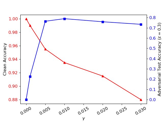
Figure A1: Clean test accuracy and adversarial test accuracy for a Small MNIST model trained with Int using different values of regularization parameter $\gamma$.

Appendix G Multi-step PGD Accuracy

Table A3 shows ATA of interpretability-aware robust training against $k$-step PGD attacks, where $k\in\{1,10,100,200\}$. As we can see, ATA decreases as $k$ increases. This again verifies that the high robust accuracy obtained from our methods is not a result of obfuscated gradients. We also see that Int outperforms IG-Norm and Int-one-class when facing stronger PGD attacks. Here the attack strength is characterized by the number of PGD steps.

Method Steps$=1$ 10 100 200 MNIST, Small, $\epsilon=0.3$ Normal 0.990 0.070 0.000 0.000 Adv 0.975 0.945 0.890 0.890 TRADES 0.970 0.955 0.885 0.885 IG-Norm 0.970 0.905 0.005 0.005 IG-Norm-Sum 0.970 0.940 0.880 0.880 Int-one-class 0.950 0.365 0.125 0.125 Int 0.935 0.910 0.790 0.790 Int-Adv 0.950 0.905 0.855 0.855 Int2 0.950 0.935 0.845 0.845 Int2-Adv 0.945 0.915 0.840 0.840 CIFAR-10, WResnet, $\epsilon=8/255$ Normal 0.470 0.075 0.060 0.060 Adv 0.590 0.205 0.185 0.185 TRADES 0.590 0.180 0.165 0.165 Int-one-class 0.505 0.100 0.060 0.060 Int 0.620 0.310 0.275 0.275 Int-Adv 0.580 0.345 0.335 0.335 Int2 0.585 0.320 0.300 0.290 Int2-Adv 0.585 0.360 0.335 0.335

Table A3: Multi-step PGD accuracy.

Appendix H Additional Tables

Method	$\epsilon=0$	0.05	0.1	0.2	0.3
MNIST, Pool
Normal	0.990	0.435	0.070	0.000	0.000
Adv	0.930	0.885	0.835	0.695	0.535
TRADES	0.955	0.910	0.870	0.720	0.455
IG-Norm	0.980	0.940	0.660	0.050	0.000
IG-Norm-Sum	0.920	0.885	0.840	0.700	0.540
Int-one-class	0.975	0.885	0.720	0.200	0.130
Int	0.950	0.930	0.875	0.680	0.390
Int-Adv	0.870	0.840	0.810	0.755	0.690
Int2	0.955	0.915	0.885	0.730	0.510
Int2-Adv	0.865	0.830	0.805	0.760	0.705
	$\epsilon=0$	2/255	4/255	6/255	8/255
CIFAR-10, Small
Normal	0.650	0.015	0.000	0.000	0.000
Adv	0.505	0.470	0.380	0.330	0.285
TRADES	0.630	0.465	0.355	0.235	0.140
IG-Norm	0.525	0.435	0.360	0.295	0.230
IG-Norm-Sum	0.390	0.365	0.325	0.310	0.285
Int-one-class	0.515	0.450	0.380	0.315	0.265
Int	0.530	0.450	0.345	0.290	0.215
Int-Adv	0.675	0.145	0.005	0.000	0.000
Int2	0.470	0.430	0.360	0.330	0.260
Int2-Adv	0.395	0.365	0.345	0.310	0.295

Table A4: 200 steps PGD accuracy, additional results.

Method	$\epsilon=0$	0.05	0.1	0.2	0.3
MNIST, Pool
Normal	0.990	0.435	0.070	0.000	0.000
Adv	0.930	0.885	0.835	0.695	0.535
TRADES	0.955	0.910	0.870	0.720	0.460
IG-Norm	0.980	0.945	0.660	0.060	0.000
IG-Norm-Sum	0.920	0.885	0.840	0.700	0.540
Int-one-class	0.975	0.885	0.720	0.200	0.130
Int	0.950	0.930	0.875	0.680	0.385
Int-Adv	0.870	0.840	0.810	0.755	0.700
Int2	0.955	0.915	0.885	0.730	0.510
Int2-Adv	0.865	0.830	0.805	0.760	0.705
	$\epsilon=0$	2/255	4/255	6/255	8/255
CIFAR-10, Small
Normal	0.650	0.015	0.000	0.000	0.000
Adv	0.505	0.470	0.380	0.330	0.285
TRADES	0.630	0.465	0.355	0.235	0.140
IG-Norm	0.525	0.435	0.360	0.295	0.230
IG-Norm-Sum	0.390	0.365	0.325	0.310	0.285
Int-one-class	0.515	0.450	0.380	0.315	0.265
Int	0.530	0.450	0.345	0.290	0.215
Int-Adv	0.675	0.145	0.005	0.000	0.000
Int2	0.470	0.430	0.360	0.330	0.260
Int2-Adv	0.395	0.365	0.345	0.310	0.295

Table A5: 100 step PGD accuracy, additional results.

Method	$\epsilon=0$	0.05	0.1	0.2	0.3
MNIST, Pool
Normal	0.990	0.470	0.135	0.135	0.135
Adv	0.930	0.885	0.845	0.845	0.845
TRADES	0.955	0.910	0.870	0.870	0.870
IG-Norm	0.980	0.945	0.705	0.705	0.705
IG-Norm-Sum	0.920	0.885	0.850	0.850	0.850
Int-one-class	0.975	0.885	0.750	0.750	0.750
Int	0.950	0.930	0.885	0.885	0.885
Int-Adv	0.870	0.840	0.810	0.810	0.810
Int2	0.955	0.915	0.885	0.885	0.885
Int2-Adv	0.865	0.830	0.805	0.805	0.805
	$\epsilon=0$	2/255	4/255	6/255	8/255
CIFAR-10, Small
Normal	0.650	0.015	0.000	0.000	0.000
Adv	0.505	0.470	0.380	0.325	0.280
TRADES	0.630	0.465	0.360	0.240	0.145
IG-Norm	0.675	0.145	0.005	0.000	0.000
IG-Norm-Sum	0.515	0.450	0.380	0.315	0.265
Int-one-class	0.530	0.450	0.345	0.290	0.220
Int	0.525	0.435	0.360	0.295	0.235
Int-Adv	0.390	0.365	0.325	0.310	0.285
Int2	0.470	0.430	0.360	0.330	0.265
Int2-Adv	0.395	0.365	0.345	0.315	0.295

Table A6: 10 step PGD accuracy, additional results.

Method	$\epsilon=0.05$	0.1	0.2	0.3
MNIST, Pool
Normal	0.934	0.876	0.719	0.482
Adv	0.976	0.951	0.896	0.824
TRADES	0.976	0.952	0.891	0.815
IG-Norm	0.942	0.872	0.648	0.341
IG-Norm-Sum	0.976	0.951	0.895	0.824
Int-one-class	0.930	0.871	0.779	0.704
Int	0.964	0.928	0.852	0.771
Int-Adv	0.977	0.957	0.921	0.891
Int2	0.969	0.941	0.885	0.832
Int2-Adv	0.977	0.956	0.921	0.889
	$\epsilon=2/255$	4/255	6/255	8/255
CIFAR-10, Small
Normal	0.694	0.350	0.116	-0.031
Adv	0.958	0.907	0.849	0.783
TRADES	0.940	0.867	0.781	0.689
IG-Norm	0.810	0.552	0.308	0.131
IG-Norm-Sum	0.958	0.907	0.847	0.779
Int-one-class	0.961	0.918	0.871	0.820
Int	0.965	0.926	0.883	0.840
Int-Adv	0.979	0.956	0.931	0.904
Int2	0.971	0.941	0.908	0.875
Int2-Adv	0.980	0.959	0.938	0.914
CIFAR-10, WResnet
Normal	0.595	0.159	0.067	-0.069
Adv	0.912	0.816	0.724	0.629
TRADES	0.918	0.832	0.747	0.652
Int	0.859	0.763	0.746	0.682
Int-Adv	0.885	0.803	0.751	0.696
Int2	0.868	0.779	0.708	0.674
Int2-Adv	0.889	0.788	0.721	0.672

Table A7: Kendall rank correlation coefficients of Top-$k$ CAM attacks against interpretability found using 200 steps of PGD, additional results.

Appendix I Additional Results on Robust Features

Seed Images Normal IG-Norm Adv Int Int2

Figure A2: Feature visualization at neuron $28$ under CIFAR-10 Small model trained by different methods.

Seed Images Normal IG-Norm Adv Int Int2

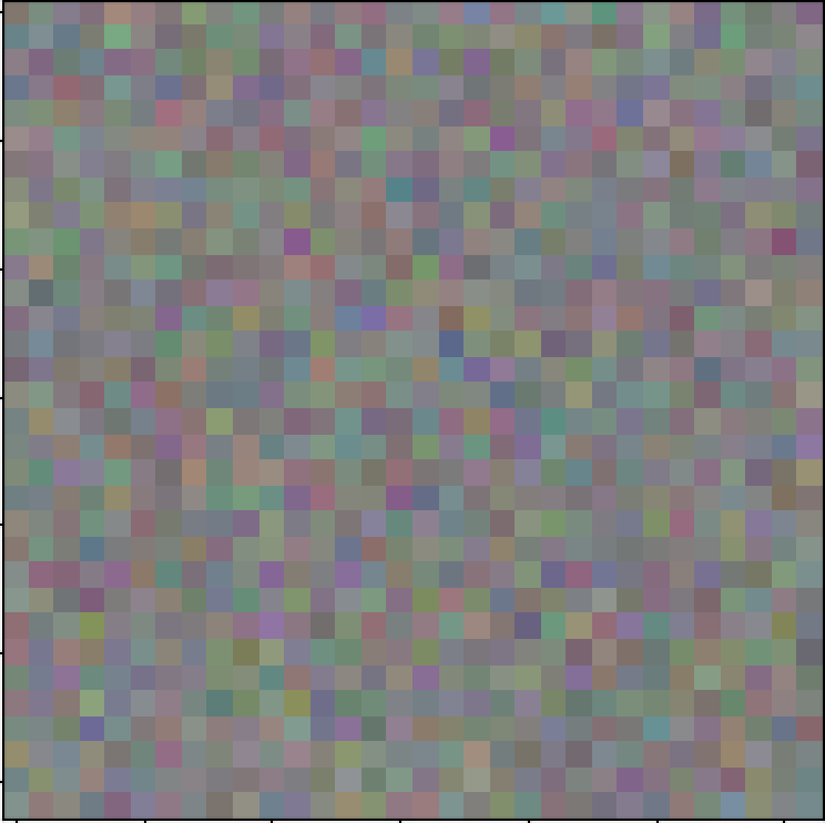
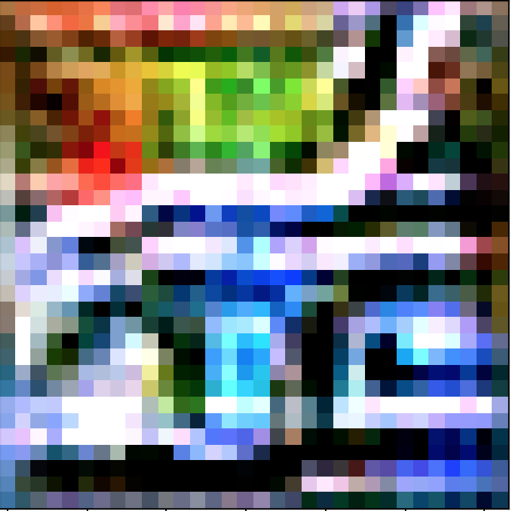
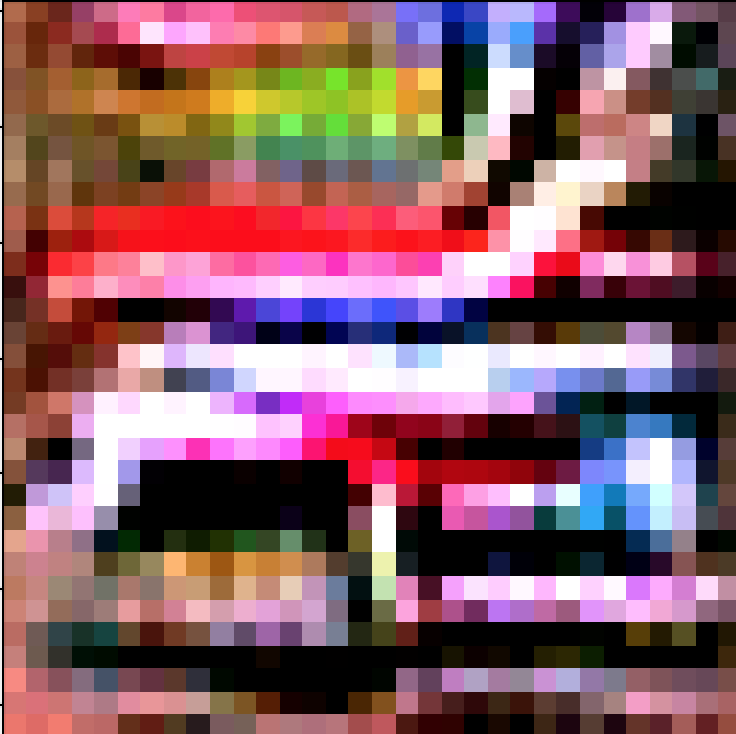
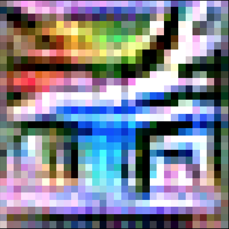
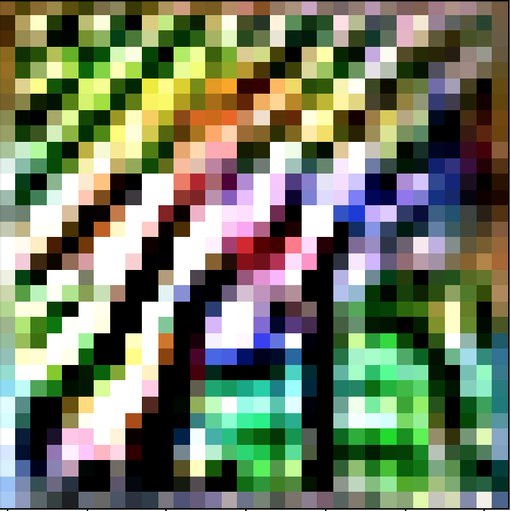
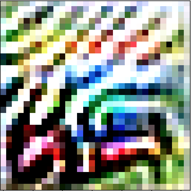
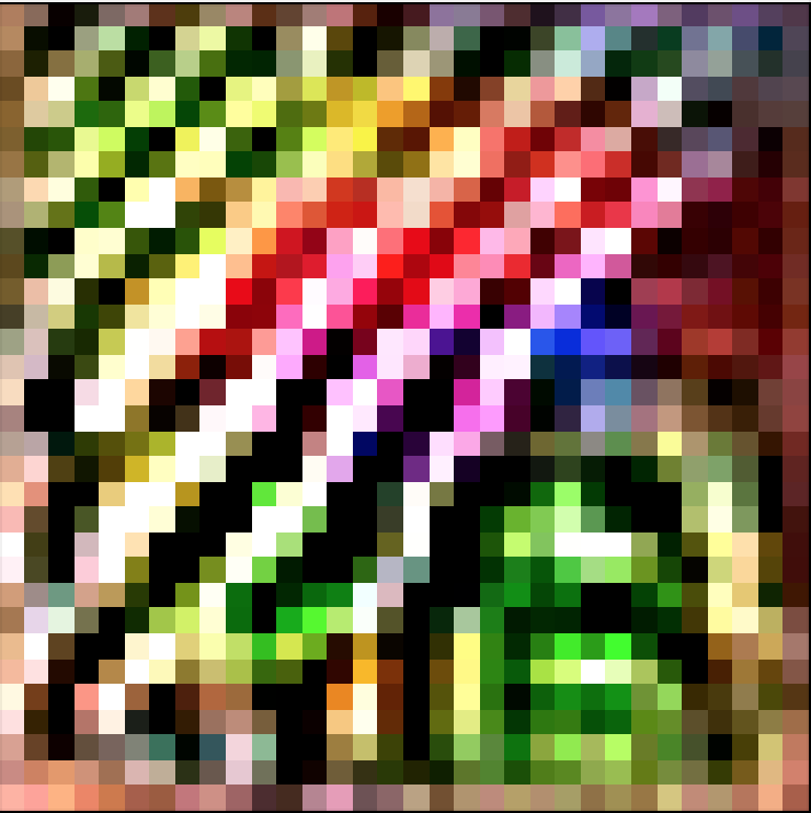
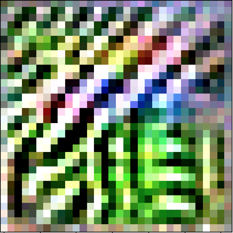
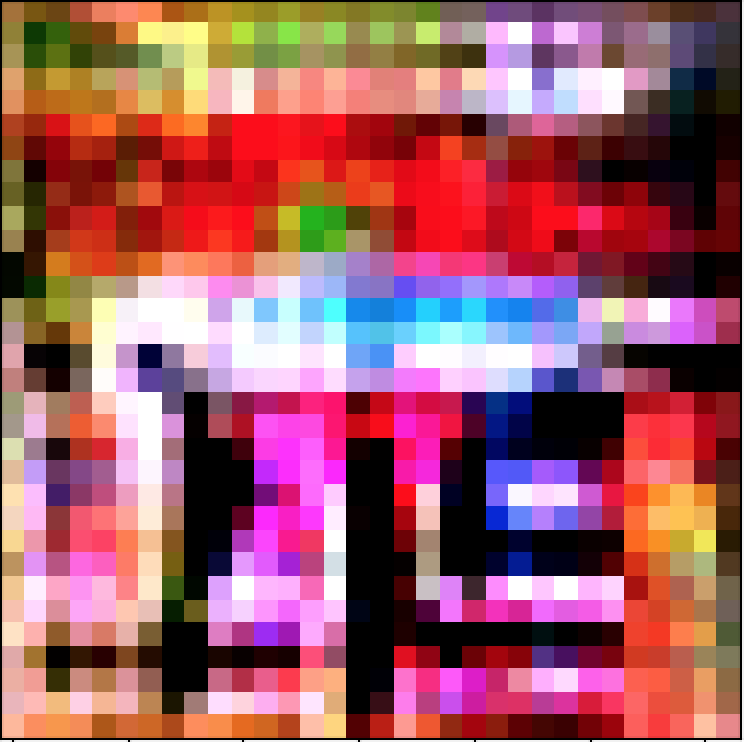
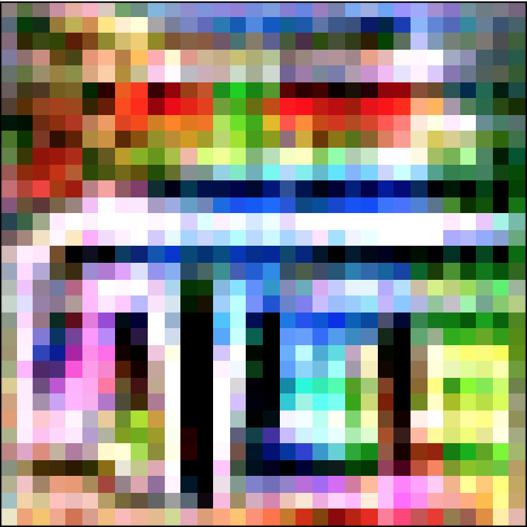
Figure A3: Feature visualization at neuron $55$ under CIFAR-10 Small model trained by different methods.

Seed Images Normal Adv Int Int2

Figure A4: Feature visualization at neuron $42$ under CIFAR-10 WResnet model trained by different methods.

Seed Images Normal Adv Int Int2

Figure A5: Feature visualization at neuron $3$ under CIFAR-10 WResnet model trained by different methods.

References

- Athalye et al. (2017) Anish Athalye, Logan Engstrom, Andrew Ilyas, and Kevin Kwok. Synthesizing robust adversarial examples. arXiv preprint arXiv:1707.07397, 2017.
- Athalye et al. (2018) Anish Athalye, Nicholas Carlini, and David Wagner. Obfuscated gradients give a false sense of security: Circumventing defenses to adversarial examples. ICML, arXiv preprint arXiv:1802.00420, 2018.
- Bau et al. (2017) David Bau, Bolei Zhou, Aditya Khosla, Aude Oliva, and Antonio Torralba. Network dissection: Quantifying interpretability of deep visual representations. In Proceedings of the IEEE Conference on Computer Vision and Pattern Recognition, pp. 6541–6549, 2017.
- Brown et al. (2017) Tom B Brown, Dandelion Mané, Aurko Roy, Martín Abadi, and Justin Gilmer. Adversarial patch. arXiv preprint arXiv:1712.09665, 2017.
- Carlini (2019) Nicholas Carlini. Is ami (attacks meet interpretability) robust to adversarial examples? arXiv preprint arXiv:1902.02322, 2019.
- Carlini & Wagner (2017) Nicholas Carlini and David Wagner. Towards evaluating the robustness of neural networks. In IEEE Symposium on Security and Privacy (SP), pp. 39–57. IEEE, 2017.
- Chattopadhay et al. (2018) Aditya Chattopadhay, Anirban Sarkar, Prantik Howlader, and Vineeth N Balasubramanian. Grad-CAM++: Generalized gradient-based visual explanations for deep convolutional networks. In 2018 IEEE Winter Conference on Applications of Computer Vision (WACV), pp. 839–847. IEEE, 2018.
- Chen et al. (2019) Jiefeng Chen, Xi Wu, Vaibhav Rastogi, Yingyu Liang, and Somesh Jha. Robust attribution regularization, 2019.
- Chen et al. (2018) Pin-Yu Chen, Yash Sharma, Huan Zhang, Jinfeng Yi, and Cho-Jui Hsieh. Ead: elastic-net attacks to deep neural networks via adversarial examples. AAAI, 2018.
- Dombrowski et al. (2019) Ann-Kathrin Dombrowski, Maximilian Alber, Christopher J Anders, Marcel Ackermann, Klaus-Robert Müller, and Pan Kessel. Explanations can be manipulated and geometry is to blame. arXiv preprint arXiv:1906.07983, 2019.
- Engstrom et al. (2019) Logan Engstrom, Andrew Ilyas, Shibani Santurkar, Dimitris Tsipras, Brandon Tran, and Aleksander Madry. Adversarial robustness as a prior for learned representations, 2019.
- Eykholt et al. (2018) K. Eykholt, I. Evtimov, E. Fernandes, B. Li, A. Rahmati, C. Xiao, A. Prakash, T. Kohno, and D. Song. Robust physical-world attacks on deep learning visual classification. In Proceedings of the IEEE Conference on Computer Vision and Pattern Recognition, pp. 1625–1634, 2018.
- Ghorbani et al. (2019) Amirata Ghorbani, Abubakar Abid, and James Zou. Interpretation of neural networks is fragile. In Proceedings of the AAAI Conference on Artificial Intelligence, volume 33, pp. 3681–3688, 2019.
- Goodfellow et al. (2015) Ian Goodfellow, Jonathon Shlens, and Christian Szegedy. Explaining and harnessing adversarial examples. ICLR, arXiv preprint arXiv:1412.6572, 2015.
- Kang et al. (2019) Daniel Kang, Yi Sun, Dan Hendrycks, Tom Brown, and Jacob Steinhardt. Testing robustness against unforeseen adversaries. arXiv preprint arXiv:1908.08016, 2019.
- Madry et al. (2018) Aleksander Madry, Aleksandar Makelov, Ludwig Schmidt, Dimitris Tsipras, and Adrian Vladu. Towards deep learning models resistant to adversarial attacks. ICLR, arXiv preprint arXiv:1706.06083, 2018.
- Moosavi-Dezfooli et al. (2019) Seyed-Mohsen Moosavi-Dezfooli, Alhussein Fawzi, Jonathan Uesato, and Pascal Frossard. Robustness via curvature regularization, and vice versa. In Proceedings of the IEEE Conference on Computer Vision and Pattern Recognition, pp. 9078–9086, 2019.
- Papernot et al. (2016a) Nicolas Papernot, Patrick McDaniel, Somesh Jha, Matt Fredrikson, Z Berkay Celik, and Ananthram Swami. The limitations of deep learning in adversarial settings. In IEEE European Symposium on Security and Privacy (EuroS&P), pp. 372–387. IEEE, 2016a.
- Papernot et al. (2016b) Nicolas Papernot, Patrick McDaniel, Xi Wu, Somesh Jha, and Ananthram Swami. Distillation as a defense to adversarial perturbations against deep neural networks. In 2016 IEEE Symposium on Security and Privacy (SP), pp. 582–597. IEEE, 2016b.
- Petsiuk et al. (2018) Vitali Petsiuk, Abir Das, and Kate Saenko. Rise: Randomized input sampling for explanation of black-box models. arXiv preprint arXiv:1806.07421, 2018.
- Ross & Doshi-Velez (2018) Andrew Slavin Ross and Finale Doshi-Velez. Improving the adversarial robustness and interpretability of deep neural networks by regularizing their input gradients. In Thirty-second AAAI conference on artificial intelligence, 2018.
- Selvaraju et al. (2017) Ramprasaath R Selvaraju, Michael Cogswell, Abhishek Das, Ramakrishna Vedantam, Devi Parikh, and Dhruv Batra. Grad-CAM: Visual explanations from deep networks via gradient-based localization. In Proceedings of the IEEE International Conference on Computer Vision, pp. 618–626, 2017.
- Simonyan et al. (2013) Karen Simonyan, Andrea Vedaldi, and Andrew Zisserman. Deep inside convolutional networks: Visualising image classification models and saliency maps. arXiv preprint arXiv:1312.6034, 2013.
- Smilkov et al. (2017) Daniel Smilkov, Nikhil Thorat, Been Kim, Fernanda Viégas, and Martin Wattenberg. Smoothgrad: removing noise by adding noise. arXiv preprint arXiv:1706.03825, 2017.
- Springenberg et al. (2014) Jost Tobias Springenberg, Alexey Dosovitskiy, Thomas Brox, and Martin Riedmiller. Striving for simplicity: The all convolutional net. arXiv preprint arXiv:1412.6806, 2014.
- Su et al. (2018) Dong Su, Huan Zhang, Hongge Chen, Jinfeng Yi, Pin-Yu Chen, and Yupeng Gao. Is robustness the cost of accuracy?–a comprehensive study on the robustness of 18 deep image classification models. arXiv preprint arXiv:1808.01688, 2018.
- Subramanya et al. (2018) Akshayvarun Subramanya, Vipin Pillai, and Hamed Pirsiavash. Towards hiding adversarial examples from network interpretation. arXiv preprint arXiv:1812.02843, 2018.
- Sundararajan et al. (2017) Mukund Sundararajan, Ankur Taly, and Qiqi Yan. Axiomatic attribution for deep networks. In Proceedings of the 34th International Conference on Machine Learning-Volume 70, pp. 3319–3328. JMLR. org, 2017.
- Szegedy et al. (2014) Christian Szegedy, Wojciech Zaremba, Ilya Sutskever, Joan Bruna, Dumitru Erhan, Ian Goodfellow, and Rob Fergus. Intriguing properties of neural networks. ICLR, arXiv preprint arXiv:1312.6199, 2014.
- Tsipras et al. (2019) Dimitris Tsipras, Shibani Santurkar, Logan Engstrom, Alexander Turner, and Aleksander Madry. Robustness may be at odds with accuracy. In International Conference on Learning Representations, 2019. URL https://openreview.net/forum?id=SyxAb30cY7.
- Xu et al. (2019a) Kaidi Xu, Sijia Liu, Gaoyuan Zhang, Mengshu Sun, Pu Zhao, Quanfu Fan, Chuang Gan, and Xue Lin. Interpreting adversarial examples by activation promotion and suppression. arXiv preprint arXiv:1904.02057, 2019a.
- Xu et al. (2019b) Kaidi Xu, Sijia Liu, Pu Zhao, Pin-Yu Chen, Huan Zhang, Quanfu Fan, Deniz Erdogmus, Yanzhi Wang, and Xue Lin. Structured adversarial attack: Towards general implementation and better interpretability. In International Conference on Learning Representations, 2019b.
- Yeh et al. (2019) Chih-Kuan Yeh, Cheng-Yu Hsieh, Arun Sai Suggala, David Inouye, and Pradeep Ravikumar. On the (in)fidelity and sensitivity for explanations, 2019.
- Zagoruyko & Komodakis (2016) Sergey Zagoruyko and Nikos Komodakis. Wide residual networks. BMVC, 2016.
- Zeiler & Fergus (2014) Matthew D Zeiler and Rob Fergus. Visualizing and understanding convolutional networks. In European conference on computer vision, pp. 818–833. Springer, 2014.
- Zhang et al. (2019) Hongyang Zhang, Yaodong Yu, Jiantao Jiao, Eric P Xing, Laurent El Ghaoui, and Michael I Jordan. Theoretically principled trade-off between robustness and accuracy. arXiv preprint arXiv:1901.08573, 2019.
- Zhang et al. (2018) Xinyang Zhang, Ningfei Wang, Shouling Ji, Hua Shen, and Ting Wang. Interpretable deep learning under fire. CoRR, abs/1812.00891, 2018. URL http://arxiv.org/abs/1812.00891.
- Zhou et al. (2016) B. Zhou, A. Khosla, A. Lapedriza, A. Oliva, and A. Torralba. Learning deep features for discriminative localization. In Proceedings of the IEEE Conference on Computer Vision and Pattern Recognition, pp. 2921–2929, 2016.