Universal two-level quantum Otto machine under a squeezed reservoir

Abstract

We study an Otto heat machine whose working substance is a single two-level system interacting with a cold thermal reservoir and with a squeezed hot thermal reservoir. By adjusting the squeezing or the adiabaticity parameter (the probability of transition) we show that our two-level system can function as a universal heat machine, either producing net work by consuming heat or consuming work that is used to cool or heat environments. Using our model we study the performance of these machine in the finite-time regime of the isentropic strokes, which is a regime that contributes to make them useful from a practical point of view.

I Introduction

Classical heat machines convert thermal resources into work and vice-versa. As for example, the heat engine draws heat from a hot reservoir, uses part of that heat to perform mechanical work and discards the rest in a cold reservoir. The refrigerator, on the other hand, uses mechanical work to remove heat from a cold reservoir and discard it in a hot one. A third kind of heat machine, the heather, uses the mechanical work to heat one, usually the cold, or both reservoirs - see Fig. 1. The cyclic heat machines are the paradigm for these comparative studies, whose efficiency $\eta$ for heat engines and coefficient of performances $COP$ for refrigerators are related by

$$COP=\frac{1}{\eta}-1.$$ (1)

Eq. (1) answers the following question: given a cyclic heat machine operating reversibly, if a work $W$ is extracted with efficiency $\eta$, what is the performance coefficient $COP$ if that same heat machine operates in a reverse cycle consuming a work $-W$. The heat machine efficiency and performance coefficient are bounded by the Carnot efficiency and performance coefficient, which, for thermal reservoirs, are only attained in quasi-static or reversible cycles. It is currently a subject of intense study to compare heat machines running on purely classic resources with heat machines running on some kind of genuinely quantum resource, as for example coherence (Scully et al., 2003, 2011; Rahav et al., 2012; Uzdin et al., 2015; Türkpençe and Müstecaplıoğlu, 2016; Brandner et al., 2017; Dorfman et al., 2018; Camati et al., 2019), entanglement (Wang et al., 2009; Correa et al., 2013; Brunner et al., 2014; Perarnau-Llobet et al., 2015; Tacchino et al., 2018), as well as exploring the finite dimension of Hilbert space (Kosloff et al., 2000; Linden et al., 2010; Gelbwaser-Klimovsky et al., 2013).

A heat machine whose working substance is a quantum system is often called a quantum heat machine. Potential technological applications of quantum heat machines ranges from heat transport in nano devices (Bermudez et al., 2013; Ronzani et al., 2018) to biological process control (Muller, 1983; Mallouk and Sen, 2009), among others (Johnson, 2014). One kind of quantum heat machine widely addressed by researchers in the field of quantum thermodynamics is the quantum Otto heat machine (QOHM) (Linden et al., 2010; Wang et al., 2012; Vinjanampathy and Anders, 2016; Karimi and Pekola, 2016; Abah and Lutz, 2016; Kosloff and Rezek, 2017; Peterson et al., 2019; Lee et al., 2020). The QOHM consists of two isochoric strokes, one with the working substance coupled to the cold thermal reservoir and the other coupled to the hot thermal reservoir, and two isentropic strokes, in which the working substance is disconnected from the thermal reservoirs and evolves unitarily. In the past years, non-thermal reservoirs have also been used in the theoretical and experimental study of QOHM, for instance squeezed thermal reservoirs (Roßnagel et al., 2014; Long and Liu, 2015; Manzano et al., 2016; Klaers et al., 2017; de Assis et al., 2020; Singh and Özgür E. Müstecaplıoğlu, 2020) and reservoirs at apparent negative temperature (de Assis et al., 2019). These unconventional quantum engines have drawn attention due to the promising gains in engine efficiency and power.

In this paper we study a minimal model of QOHM which is universal (Gelbwaser-Klimovsky et al., 2013; Myers and Deffner, 2020) in the sense that it can works either as a heat engine or a refrigerator or, yet, a heater – see Fig. 1, depending on the control parameter. Our model consists of a two-level system (TLS) driven by an external laser source and interacting with a cold thermal reservoir and with a squeezed hot thermal reservoir, which will be assumed as a free resource (Klaers et al., 2017). The relation between $\eta$ and $COP$ (Eq. (1)) will be generalized to include the squeezing parameter, which will be our parameter of control in building these types of heat machines. Using our model, we are able to study both the efficiency and performance of this TLS machine at finite-time regime of the isentropic strokes, which contributes to making them useful from the point of view of applicability.

This paper is organized as follows. In Sec. II we present our model for a universal QOHM, which consists of a TLS as the working substance under a cold thermal and a squeezed hot thermal reservoir. In Sec. III we present the results of our calculation for the heats exchanged with the reservoirs and the work done or performed by the QOHM and the corresponding efficiency $\eta$ and performance coefficient $COP$. In Sec. IV we generalize the relation between $\eta$ and $COP$ given by Eq. (1) to include both the squeezed thermal reservoir and finite-time isentropic strokes. Finally, in Sec. V we present our conclusions.

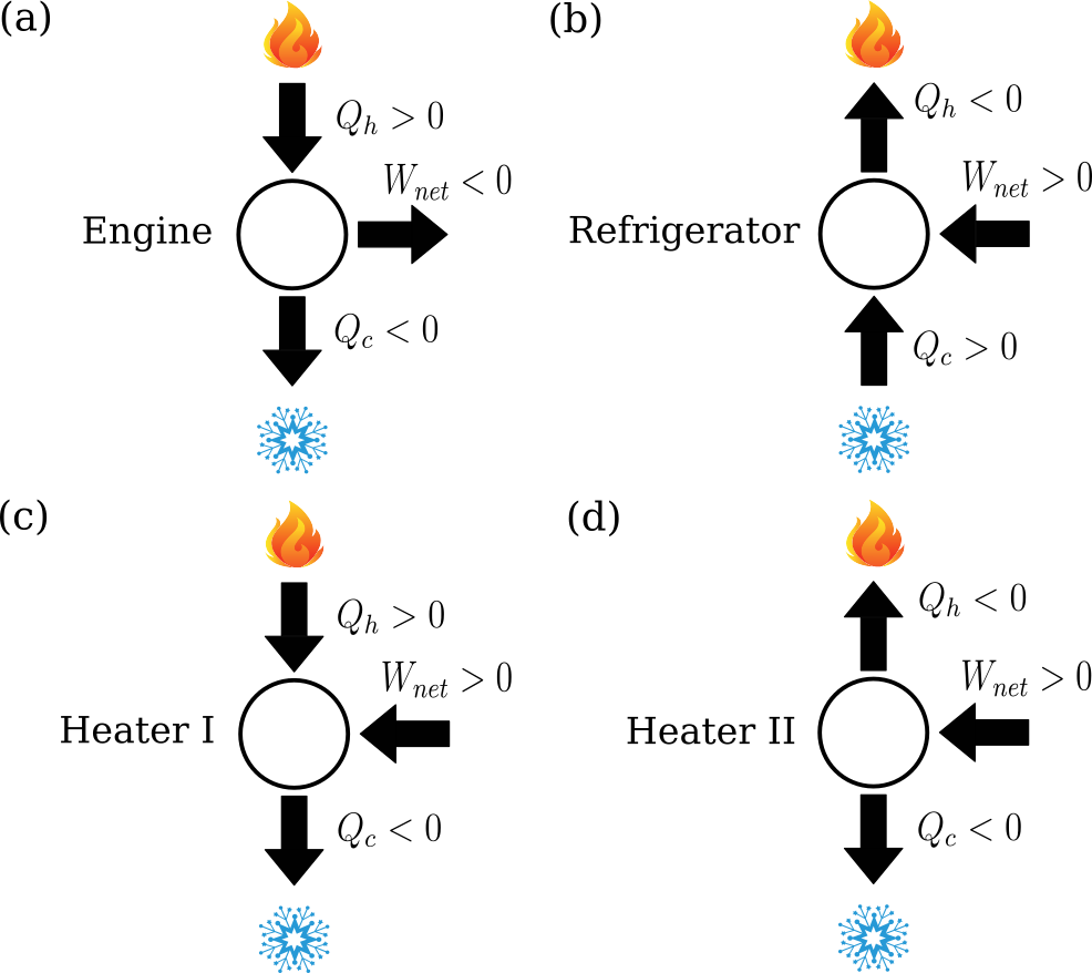
Figure 1: The four types of heat machines: (a) a heat engine, which draws heat from the hot reservoir and dumps it in the cold one, performing work, (b) a refrigerator, on which work is performed and used to draw heat from the cold reservoir and pump it to the hot one, (c) a heater that uses the work done to pump heat from the hot to the cold reservoir, and (d) a second type of heat machine that uses the work done to heat two environments at once.

II Universal QOHM

We are going to consider the TLS implementation of a four-stroke quantum Otto cycle. The four-stroke to our QOHM are the following:

(i) Cooling stroke. In this first step, the TLS is weakly coupled to the cold thermal reservoir until thermalized, when it can be described by the Gibbs state $\rho_{1}^{G}=\text{e}^{-\beta_{c}H_{c}}/\text{Tr}\left(\text{e}^{-\beta_{c}H_{c}}\right)$, where $H_{c}$ is the Hamiltonian and $\beta_{c}=1/k_{B}T_{c}$, where $k_{B}$ is the Boltzmann constant and $T_{c}$ is the reservoir temperature. The TLS Hamiltonian remains unchanged during the thermalization process and has the form $H_{c}=\frac{1}{2}\hbar\omega_{c}\sigma_{x}$, with $\hbar$, $\omega_{c}$, and $\sigma_{x}$ being the reduced Planck constant, the angular frequency, and the x Pauli matrix, respectively.

(ii) Expansion stroke. In this stage the TLS evolves unitarily from the state $\rho_{1}^{G}$ (at time $t=0$) to $\rho_{2}=U\rho_{1}^{G}U^{\dagger}$(at time $t=\tau$), where $U$ is the unitary operator accounting for the external driven of the TLS Hamiltonian, which varies from $H_{c}=\frac{1}{2}\hbar\omega_{c}\sigma_{x}$ to $H_{h}=\frac{1}{2}\hbar\omega_{h}\sigma_{y}$, with $\omega_{h}$ being an angular frequency higher then $\omega_{c}$ (corresponding to the energy gap expansion). For our purpose, it is not necessary to specify the unitary operator $U$.

(iii) Heating stroke. This is the stage where the TLS is weakly coupled to the hot squeezed thermal reservoir until reaching the stead state $\rho_{3}^{S}=S\rho_{3}^{G}S^{\dagger}$. The reservoir squeezing changes the thermalized state $\rho_{3}^{G}=\text{e}^{-\beta_{h}H_{h}}/\text{Tr}\left(\text{e}^{-\beta_{h}H_{h}}\right)$ according to operator $S=\left(\mu\left|-_{y}\right\rangle\left\langle+_{y}\right|+\nu\left|+_{y}\right\rangle\left\langle-_{y}\right|\right)/\sqrt{\mu^{2}+\nu^{2}}$, where $\mu=\cosh r$ and $\nu=\sinh r$ (Srikanth and Banerjee, 2008). The state $\left|-_{y}\right\rangle$ ($\left|+_{y}\right\rangle$) is the ground (excited) state of the TLS at this stage, and $r$ is the squeezing parameter. As in the cooling stroke, here the TLS Hamiltonian $H_{h}=\frac{1}{2}\hbar\omega_{h}\sigma_{y}$ also remains unchanged.

(iv) Compression stroke. This stage is accomplished by reversing the expansion protocol (ii), such that the TLS Hamiltonian is changed from $H_{h}=\frac{1}{2}\hbar\omega_{h}\sigma_{y}$ to $H_{c}=\frac{1}{2}\hbar\omega_{c}\sigma_{x}$, corresponding to the energy gap compression, making the TLS state to evolve unitarily from to $\rho_{3}^{S}$ to $\rho_{4}=U^{\dagger}\rho_{3}^{S}U$.

The quantities we are interested in is the efficiency $\eta$ to the heat engine as well as the coefficient of performance $COP$ to the refrigerator. The engine efficiency is given by $\eta=-W_{net}/Q_{h}$, where $Q_{h}$ is the average heat absorbed from the hot reservoir and $W_{net}$ is the average net work extracted from the engine, while the coefficient of performance, on the other hand, is given by $COP=Q_{c}/W_{net}$, where $Q_{c}$ is the average heat extracted from the cold thermal reservoir by performing an average net work $W_{net}$ on the TLS. In order to determine both the efficiency and the coefficient of performance we resort to the first law of thermodynamics, together with work and heat definitions, as follows. According to the first law of thermodynamics, the change in the internal energy of a given system during a thermodynamic process can be decomposed into work $W$ and heat $Q$. In quantum thermodynamics the first law is written as $\Delta E=Q+W$, where $\Delta E$ is the average change in the system internal energy, which is given by $E=\text{Tr}\left(\rho H\right)$. Heat and work averages, in turn, are $Q=\int dt\text{Tr}\left[\left(d\rho/dt\right)H\right]$ and $W=\int dt\text{Tr}\left[\rho\left(dH/dt\right)\right]$ (Alicki, 1979; Kosloff, 1984), respectively. Therefore, according to the first law, from the quantum Otto cycle described in (i)-(iv), we can promptly see that $W=0$ and $\Delta E=Q$ in the heating and cooling strokes, and $Q=0$ and $\Delta E=W$ in the expansion and compression strokes. This considerably simplifies the calculations, as compared to other cyclic machines as for example Carnot or Stirling, where work and heat are simultaneously exchanged.

Aiming at possible applications in nuclear magnetic resonance (Peterson et al., 2019; de Assis et al., 2019), we use here the following parameters in our numerical calculations: $\omega_{c}=2\pi$ kHz, $\omega_{h}=3.5\omega_{c}$, $\beta_{c}=1/\left(10\ \text{peV}\right)$ , and $\beta_{h}=0.7\beta_{c}$.

III Results

With the information provided in (i)-(iv) strokes and definitions of work and heat as given in Sec. II, we can obtain the average heats exchanged with the cold and hot reservoirs as well as the average net work:

$$Q_{c}=-\frac{1}{2}\hbar\omega_{c}\left(\tanh\theta_{c}-\zeta\tanh\theta_{h}\right)-\hbar\xi\zeta\omega_{c}\tanh\theta_{h}$$ (2)

$$Q_{h}=\frac{1}{2}\hbar\omega_{h}\left(\tanh\theta_{c}-\zeta\tanh\theta_{h}\right)-\hbar\xi\omega_{h}\tanh\theta_{c},$$ (3)

and

$$W_{net}=-\frac{1}{2}\hbar\left(\omega_{h}-\omega_{c}\right)\left(\tanh\theta_{c}-\zeta\tanh\theta_{h}\right)\\ +\hbar\xi\left(\omega_{h}\tanh\theta_{c}+\zeta\omega_{c}\tanh\theta_{h}\right),$$ (4)

where $\theta_{c\left(h\right)}=\frac{1}{2}\beta_{c\left(h\right)}\hbar\omega_{c\left(h\right)}$, $\zeta=1/\left(\mu{}^{2}+\nu{}^{2}\right)^{2}$ and $\xi=\left|\langle\pm_{y}|U|\mp_{x}\rangle\right|^{2}=\left|\langle\pm_{x}|U^{\dagger}|\mp_{y}\rangle\right|^{2}$. The parameter $\xi$, which gives the probability of transition between the two levels of the TLS, is the adiabaticity parameter (de Assis et al., 2019; Peterson et al., 2019). This parameter allows us to study the QOHM efficiency and performance coefficient in any time regime. In fact, this so-called adiabaticity parameter is the transition probability induced by the unitary evolution $U$, and the faster the unitary process the greater $\xi$. When $\xi=0$, the process is called quasi-static and occurs at null power. Finite-time processes, on the other hand, occurs at non-null power, and for instantaneous process $U=I$, with $I$ being the identity. As we shall see, the Otto efficiency and performance coefficient occurs to $\xi=0$, corresponding to a machine operating at null power. As we are not attaching any secondary system to exchange work with our TLS machine, either in the case of heat engines or the in the case of refrigerators, we can think about this simplified model as a proof or concept (Peterson et al., 2019), allowing us to impose theoretically maximum constraints on their efficiency or performance coefficient.

According to our convention, $Q>0$ ($Q<0$) means heat energy flowing into (out of) the engine, while $W_{net}<0$ ($W_{net}>0$) means useful energy flowing out of (into) the engine - see Fig. 1. In Fig. 2 we show all the three relevant quantities $Q_{c}$ (dotted blue line), $Q_{h}$ (dashed red line) and $W_{net}$ (solid black line) versus the squeezing parameter $r$ for $\xi=0$ (Fig. 2(a)) and $\xi=0.2$ (Fig. 2(b)). From Fig. 2(a) the universality of our TLS machine should be apparent. For example, if we want to build a heat engine, for which $Q_{c}<0$, $Q_{h}>0$ and $W_{net}<0$, then we should choose $r\apprge 0.77$; if we want to build a refrigerator, for which $Q_{h}<0$, $Q_{c}>0$ and $W_{net}>0$ then our control parameter should be $r\apprle 0.29$; heater machines of types I and II, on the other hand, lies in region $0.29\apprle r\apprle 0.77$, thus corresponding to the four types of heat machines as shown in Fig. 1. Also, note from Fig. 2(b) that to the quasi-static case $\xi=0$ there are only two types of heat machines, and depending on the value of $r$, the machine switches directly from engine to refrigerator and vice-versa.

In the following sections we will study the two main types of machines whose application has been highlighted in the most varied contexts, which are the engine and the refrigerator, by considering the squeezing as the control parameter.

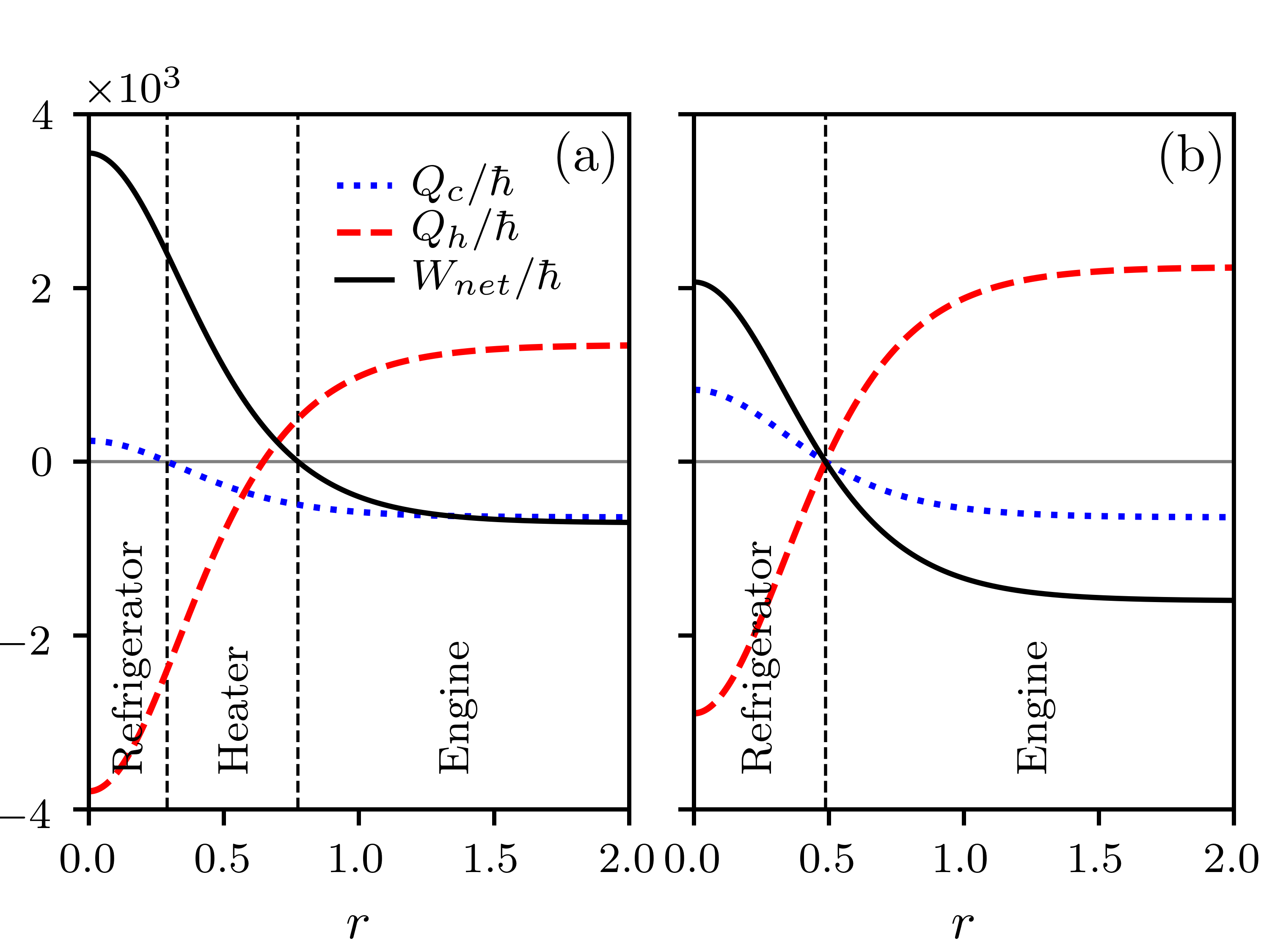
Figure 2: Curves $Q_{c}$ (dotted blue line) $Q_{h}$ (dashed red line) and $W_{net}$ (solid black line) versus the squeezing parameter $r$. These curves highlight the universality of our model, since depending on the value of the control parameter $r$ the four types of machines shown in Fig. 1 can be engineered. The parameters used here are (a) $\xi=0.2$, $\omega_{c}=2\pi$ kHz, $\omega_{h}=3.5\omega_{c}$, $\beta_{c}=1/\left(10\ \text{peV}\right)$ , $\beta_{h}=0.7\beta_{c}$, and (b) $\xi=0$, $\omega_{c}=2\pi$ kHz, $\omega_{h}=3.5\omega_{c}$, $\beta_{c}=1/\left(10\ \text{peV}\right)$ , $\beta_{h}=0.7\beta_{c}$. Dotted black lines delimit the regions of the different types of machine shown in Fig. 1.

III.1 Two-level heat engine

Following the definition of efficiency, which is $\eta=-W_{net}/Q_{h}$, we find to our model:

$$\eta=1-\frac{\omega_{c}}{\omega_{h}}\mathcal{R},$$ (5)

where

$$\mathcal{R}=\frac{1+2\xi{\cal F}}{1-2\xi{\cal G}},$$ (6)

with

$${\cal F}=\frac{\zeta\text{tanh}\theta_{h}}{\text{tanh}\theta_{c}-\zeta\text{tanh}\theta_{h}}$$ (7)

and

$${\cal G}=\frac{\text{tanh}\theta_{c}}{\text{tanh}\theta_{c}-\zeta\text{tanh}\theta_{h}}.$$ (8)

Note, from Eq. (6), that $\mathcal{R}=1$ when $\xi=0$, which corresponds to the quasi-static case, and $\eta=1-\frac{\omega_{c}}{\omega_{h}}\equiv\eta_{Otto}$.

In terms of the adiabaticity parameter $\xi$ the condition to extract work is $W_{net}<0$, such that

$$\xi<\frac{\left(\omega_{h}-\omega_{c}\right)\left(\tanh\theta_{c}-\zeta\tanh\theta_{h}\right)}{2\left(\omega_{h}\tanh\theta_{c}+\zeta\omega_{c}\tanh\theta_{h}\right)},$$ (9)

which implies $\zeta<\tanh\theta_{c}/\tanh\theta_{h}$ (since $\xi\geq 0$). As we can confirm both analytically and numerically, this condition results in heat absorption from the squeezed hot thermal reservoir, $Q_{h}>0$, and heat loss to the cold thermal reservoir, $Q_{c}<0$, which characterizes the heat engine. In Fig. 3 we show the efficiency $\eta$ versus the squeezing parameter for quasi-static regime $\xi=0$ (solid black line), which gives the Otto efficiency, and for finite-time regime $\xi=0.1$ (dashed blue line) and $\xi=0.2$ (dotted red line). Fig. 3 shows that although the engine efficiency can be enhanced by the squeezed reservoir, the Otto efficiency is never achieved for processes occurring in finite-time regimes. However, for a treatment of the engine efficiency when elaborated optimization procedure is carried out, see Ref. (de Assis et al., 2020).

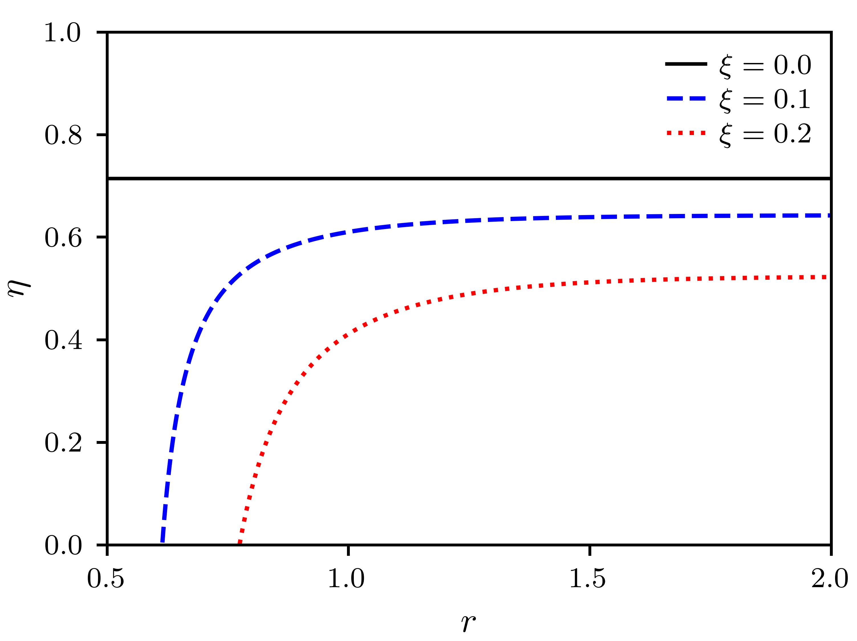
Figure 3: Efficiency $\eta$ to the TLS engine versus the squeezing parameter $r$ considering quasi-static processes $\xi=0$, resulting in the Otto efficiency $\eta_{Otto}=1-\omega_{c}/\omega_{h}$ (horizontal solid black line), and the finite-time regime $\xi=0.1$ (dashed blue line) and $\xi=0.2$ (dotted red line). We also use the parameters $\omega_{c}=2\pi$ kHz, $\omega_{h}=3.5\omega_{c}$, $\beta_{c}=1/\left(10\ \text{peV}\right)$, and $\beta_{h}=0.7\beta_{c}$.

III.2 Two-level Refrigerator

According to Eq. (1), a good engine is a poor refrigerator and vice-versa. This leads us to the conclusion that, as we have seen in the previous Section, since the squeezing parameter enhances the engine efficiency, squeezed reservoirs should not enhance the coefficient of performance. As we shall see, our results confirm that this is true. The refrigerator $COP$ is defined by the ratio $COP=Q_{c}/W_{net}$, meaning that the goal is to extract as much heat as possible from the cold reservoir by doing a minimum of work. From Eqs. (2) and (4) we obtain

$$COP=\frac{\omega_{c}\left(\tanh\theta_{c}-\zeta\tanh\theta_{h}\right)-\xi\zeta\omega_{c}\tanh\theta_{h}}{\left(\omega_{h}-\omega_{c}\right)\left(\tanh\theta_{c}-\zeta\tanh\theta_{h}\right)+\xi\left(\omega_{h}\tanh\theta_{c}+\zeta\omega_{c}\tanh\theta_{h}\right)}$$ (10)

or, after a little algebra:

$$COP=\frac{\mathcal{R}COP_{Otto}}{1+COP_{Otto}\left(1-\mathcal{R}\right)},$$ (11)

where $\mathcal{R}$ was defined in Eqs. (6)-(8) and

$$COP_{Otto}=\frac{\omega_{c}}{\omega_{h}-\omega_{c}}$$ (12)

is the ideal $COP$ obtained from quasi-static processes, i.e., by letting $\xi=0$ ($\mathcal{R}=1$).

Recalling that Eq. (11) makes sense only for $Q_{c}>0$ and $W_{net}>0$ , the following constraint must be obeyed:

$$\xi<\frac{1}{2}\left(1-\frac{\tanh\theta_{c}}{\zeta\tanh\theta_{h}}\right).$$ (13)

By imposing the constraint Eq. (13), we can numerically verify that the highest value of $COP$ is equal to the ideal Otto machine $COP_{Otto}=\omega_{c}/\left(\omega_{h}-\omega_{c}\right)$, which occurs to the quasi-static process $\xi=0$ or $\mathcal{R}=1$. In Fig. 4 we show the $COP$ for the ideal Otto refrigerator $\xi=0$, solid black line, as well as for two other finite-time parameters $\xi=0.1$ (dashed blue line) and $\xi=0.2$ (dotted red line). As we can see, for $\xi>0$ all curves in Fig. 4 start below the ideal Otto performance coefficient $COP_{Otto}=0.4$ and decreases further as the squeezing parameter increases. As expected, the performance coefficient behavior is contrary to the efficiency behavior shown in Fig. 3.

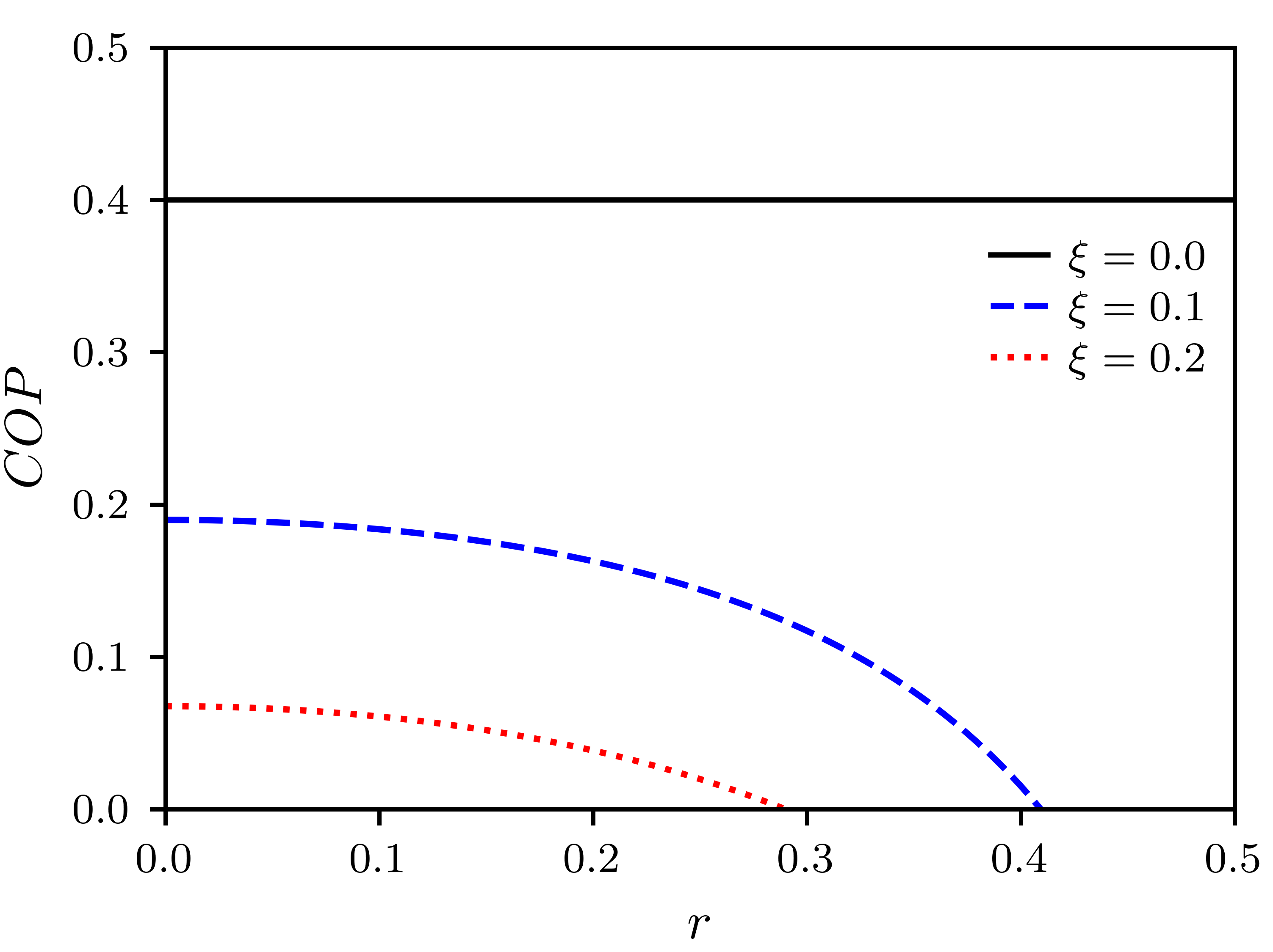
Figure 4: Performance COP versus the parameter $r$ of the squeezed reservoir for a (a) quasi-static process $\xi=0$, solid black line, and finite time processes (b) $\xi=0.1$, dashed blue line, and (c) $\xi=0.2$, dotted red line. The other parameters used here are $\omega_{c}=2\pi$ kHz, $\omega_{h}=3.5\omega_{c}$, $\beta_{c}=1/\left(10\ \text{peV}\right)$, and $\beta_{h}=0.7\beta_{c}$.

IV Generalized relation between $\eta$ and $COP$

In this Section we will generalize Eq. (1) to take into account processes occurring at $\xi>0$ and under squeezed reservoirs. To this end, we eliminate $W_{net}$ from both $\eta=-W_{net}/Q_{h}$ and $COP=Q_{c}/W_{net}$ using Eqs. (2)-(4), to obtain

$$COP=\frac{1}{\eta}\frac{\omega_{c}}{\omega_{h}}\frac{\left[\tanh\left(\theta_{c}\right)-\zeta\tanh\left(\theta_{h}\right)\right]+2\xi\zeta\tanh\left(\theta_{h}\right)}{\left[\tanh\left(\theta_{c}\right)-\zeta\tanh\left(\theta_{h}\right)\right]+2\xi\tanh\left(\theta_{c}\right)},$$ (14)

or, using $\eta_{Otto}=1-\frac{\omega_{c}}{\omega_{h}}$ and $\mathcal{R}$ as defined by Eqs. (1)-(8):

$$COP=\left(\frac{1}{\eta}-\frac{\eta_{Otto}}{\eta}\right)\mathcal{R}.$$ (15)

Note that for $\xi=0$ it is always possible to obtain a relation between $\eta$ and $COP$, since $\mathcal{R}=1$ and hence $COP=COP_{Otto}$ and $\eta=\eta_{Otto}$:

$$COP_{Otto}=\frac{1}{\eta_{Otto}}-1,$$ (16)

which is exactly the same as Eq. (1) and, therefore the squeezing parameter does not modify the relation between $\eta$ and $COP$ in the quasi-static limit. However, for $\xi>0$ it should be noted that, except for a narrow region, see Fig. 2(a), in different regions in which the heat machine operates either as refrigerator or engine, the parameters for which $W_{net}>0$ are not the same as those for $W_{net}<0$, thus implying that it is not legitimate to consider $W_{net}^{\left(engime\right)}=-W_{net}^{\left(fridge\right)}$. As a consequence, unlike what happens in the quasi-static case shown in Fig. 2(b), for $\xi>0$ there will not always be a balance between the work $W_{net}$ that can be extracted from a universal TLS engine having $\eta$ efficiency, and the COP performance that would be obtained if that same work $W_{net}$ were supplied to a fridge machine.

V Conclusion

We have proposed a universal quantum Otto heat machine (QOHM) based on a two-level system as the working substance that operates under two reservoirs: a cold thermal reservoir and a squeezed hot thermal reservoir. For universal QOHM we mean the possibility of changing the parameters of control, such as the squeezing $r$ and the adiabaticity $\xi$ parameters, to make the machine work either as a thermal engine, or as a refrigerator, or as a heater. We also showed that the squeezing parameter, although useful to improve the efficiency of an engine, always leads to a worsening of the performance coefficient of a refrigerator. This is in contrast with the result from Ref. (Long and Liu, 2015), where the authors considered a harmonic oscillator as the work substance and the cold reservoir as the squeezed one. Finally, we have demonstrated that the usual relation between $\eta$ and $COP$, Eq. (1), remains unchanged for a heat machine working at null power under two reservoirs: a cold thermal reservoir and a hot squeezed thermal reservoir.

References

- Scully et al. (2003) M. O. Scully, M. S. Zubairy, G. S. Agarwal, and H. Walther, Science 299, 862 (2003), https://science.sciencemag.org/content/299/5608/862.full.pdf .
- Scully et al. (2011) M. O. Scully, K. R. Chapin, K. E. Dorfman, M. B. Kim, and A. Svidzinsky, Proceedings of the National Academy of Sciences 108, 15097 (2011), https://www.pnas.org/content/108/37/15097.full.pdf .
- Rahav et al. (2012) S. Rahav, U. Harbola, and S. Mukamel, Phys. Rev. A 86, 043843 (2012).
- Uzdin et al. (2015) R. Uzdin, A. Levy, and R. Kosloff, Phys. Rev. X 5, 031044 (2015).
- Türkpençe and Müstecaplıoğlu (2016) D. Türkpençe and O. E. Müstecaplıoğlu, Phys. Rev. E 93, 012145 (2016).
- Brandner et al. (2017) K. Brandner, M. Bauer, and U. Seifert, Phys. Rev. Lett. 119, 170602 (2017).
- Dorfman et al. (2018) K. E. Dorfman, D. Xu, and J. Cao, Phys. Rev. E 97, 042120 (2018).
- Camati et al. (2019) P. A. Camati, J. F. G. Santos, and R. M. Serra, Phys. Rev. A 99, 062103 (2019).
- Wang et al. (2009) H. Wang, S. Liu, and J. He, Phys. Rev. E 79, 041113 (2009).
- Correa et al. (2013) L. A. Correa, J. P. Palao, G. Adesso, and D. Alonso, Phys. Rev. E 87, 042131 (2013).
- Brunner et al. (2014) N. Brunner, M. Huber, N. Linden, S. Popescu, R. Silva, and P. Skrzypczyk, Phys. Rev. E 89, 032115 (2014).
- Perarnau-Llobet et al. (2015) M. Perarnau-Llobet, K. V. Hovhannisyan, M. Huber, P. Skrzypczyk, N. Brunner, and A. Acín, Phys. Rev. X 5, 041011 (2015).
- Tacchino et al. (2018) F. Tacchino, A. Auffèves, M. F. Santos, and D. Gerace, Phys. Rev. Lett. 120, 063604 (2018).
- Kosloff et al. (2000) R. Kosloff, E. Geva, and J. M. Gordon, Journal of Applied Physics 87, 8093 (2000), https://doi.org/10.1063/1.373503 .
- Linden et al. (2010) N. Linden, S. Popescu, and P. Skrzypczyk, Phys. Rev. Lett. 105, 130401 (2010).
- Gelbwaser-Klimovsky et al. (2013) D. Gelbwaser-Klimovsky, R. Alicki, and G. Kurizki, Phys. Rev. E 87, 012140 (2013).
- Bermudez et al. (2013) A. Bermudez, M. Bruderer, and M. B. Plenio, Phys. Rev. Lett. 111, 040601 (2013).
- Ronzani et al. (2018) A. Ronzani, B. Karimi, J. Senior, Y.-C. Chang, J. T. Peltonen, C. Chen, and J. P. Pekola, Nature Physics 14, 991 (2018).
- Muller (1983) A. W. Muller, Physics Letters A 96, 319 (1983).
- Mallouk and Sen (2009) T. Mallouk and A. Sen, Scientific American 300, 72 (2009).
- Johnson (2014) C. V. Johnson, Classical and Quantum Gravity 31, 205002 (2014).
- Wang et al. (2012) J. Wang, Z. Wu, and J. He, Phys. Rev. E 85, 041148 (2012).
- Vinjanampathy and Anders (2016) S. Vinjanampathy and J. Anders, Contemporary Physics 57, 545 (2016), https://doi.org/10.1080/00107514.2016.1201896 .
- Karimi and Pekola (2016) B. Karimi and J. P. Pekola, Phys. Rev. B 94, 184503 (2016).
- Abah and Lutz (2016) O. Abah and E. Lutz, EPL (Europhysics Letters) 113, 60002 (2016).
- Kosloff and Rezek (2017) R. Kosloff and Y. Rezek, Entropy 19, 136 (2017).
- Peterson et al. (2019) J. P. S. Peterson, T. B. Batalhão, M. Herrera, A. M. Souza, R. S. Sarthour, I. S. Oliveira, and R. M. Serra, Phys. Rev. Lett. 123, 240601 (2019).
- Lee et al. (2020) S. Lee, M. Ha, J.-M. Park, and H. Jeong, Phys. Rev. E 101, 022127 (2020).
- Roßnagel et al. (2014) J. Roßnagel, O. Abah, F. Schmidt-Kaler, K. Singer, and E. Lutz, Phys. Rev. Lett. 112, 030602 (2014).
- Long and Liu (2015) R. Long and W. Liu, Phys. Rev. E 91, 062137 (2015).
- Manzano et al. (2016) G. Manzano, F. Galve, R. Zambrini, and J. M. R. Parrondo, Phys. Rev. E 93, 052120 (2016).
- Klaers et al. (2017) J. Klaers, S. Faelt, A. Imamoglu, and E. Togan, Phys. Rev. X 7, 031044 (2017).
- de Assis et al. (2020) R. J. de Assis, J. S. Sales, U. C. Mendes, and N. G. de Almeida, (2020), arXiv:2003.12664 .
- Singh and Özgür E. Müstecaplıoğlu (2020) V. Singh and Özgür E. Müstecaplıoğlu, (2020), arXiv:2006.08311 .
- de Assis et al. (2019) R. J. de Assis, T. M. de Mendonça, C. J. Villas-Boas, A. M. de Souza, R. S. Sarthour, I. S. Oliveira, and N. G. de Almeida, Phys. Rev. Lett. 122, 240602 (2019).
- Myers and Deffner (2020) N. M. Myers and S. Deffner, Phys. Rev. E 101, 012110 (2020).
- Srikanth and Banerjee (2008) R. Srikanth and S. Banerjee, Phys. Rev. A 77, 012318 (2008).
- Alicki (1979) R. Alicki, Journal of Physics A: Mathematical and General 12, L103 (1979).
- Kosloff (1984) R. Kosloff, The Journal of Chemical Physics 80, 1625 (1984), https://doi.org/10.1063/1.446862 .