A Computational Model of Protein Induced Membrane Morphology with Geodesic Curvature Driven Protein-Membrane Interface

Abstract

Continuum or hybrid modeling of bilayer membrane morphological dynamics induced by embedded proteins necessitates the identification of protein-membrane interfaces and coupling of deformations of two surfaces. In this article we developed (i) a minimal total geodesic curvature model to describe these interfaces, and (ii) a numerical one-one mapping between two surface through a conformal mapping of each surface to the common middle annulus. Our work provides the first computational tractable approach for determining the interfaces between bilayer and embedded proteins. The one-one mapping allows a convenient coupling of the morphology of two surfaces. We integrated these two new developments into the energetic model of protein-membrane interactions, and developed the full set of numerical methods for the coupled system. Numerical examples are presented to demonstrate (1) the efficiency and robustness of our methods in locating the curves with minimal total geodesic curvature on highly complicated protein surfaces, (2) the usefulness of these interfaces as interior boundaries for membrane deformation, and (3) the rich morphology of bilayer surfaces for different protein-membrane interfaces.

1 Introduction

Lipid bilayer membranes are highly curved macromolecules whose curvatures have been long recognized as an essential structural feature in key biological processes such as membrane trafficking, cytokinesis, infection, and cell motion. Biological membranes, however, are far more complicated than simple bilayers because of the presence of non-lipid components, in particular, proteins. Measured by weight, the ratio of protein to lipid is about $0.2$ in myelin, while in the mitochondrial inner membrane the ratio is about 3.0 [1]. More recent measurements identified about $40$ different membrane proteins in the membrane of a synaptic vesicle with a diameter around $40$ nm [2]. Generation, modulation, and maintenance of biological membrane curvature is therefore intrinsically coupled to the interactions between lipid bilayers and membrane proteins. These interactions also determine the conformational change of transmembrane segments of membrane proteins [3], see for example the gating of mechanosensitive ion channels [4]. The importance and complexity of protein-mediated membrane morphological variation has thus fascinated investigators from various backgrounds.

In this article we develop a hybrid computational model of protein embedding into bilayer membrane for quantifying two critical geometric features of protein-membrane interactions. These are (i) the interface between bilayer and the embedded protein, and (ii) the surface morphology of the bilayer with the embedded protein. This interface sets a boundary for the lipid bilayer whose deformation will produce a tensional force on the boundary that shall displace the interface as a feedback, thus defining a bidirectional coupling between membrane morphological changes and the state of protein inclusion. Different treatments exist for these two features. Continuum [5] or hybrid [6, 7, 8, 9, 10] models usually treat the whole bilayer or its two individual leaflets as an elastic sheet using the classical Helfrich theory [11, 12, 13] or Monge parameterization. An explicit specification of membrane edge and the boundary condition for displacement are in these models. In fully atomistic [14] or coarse-grained [15, 8] models it is not necessary to explicitly track the protein-membrane interface or membrane surface as they arise naturally as a result of trajectories of particles under simulations. However, it still remains a grand challenge for full atomistic or coarse-grained molecular dynamics simulators to model protein modulated membrane deformations or membrane mediated protein conformation changes of biologically relevant spatial and time scales [16]. Continuum or hybrid models appear attractive for tackling these problems for they can be scaled to large domains and long time simulations at a relatively low computational cost.

Description of protein membrane interfaces and boundary conditions for membrane elasticity vary in complexity and detail. For example, in [15, 17] the channel protein is represented as cylindrical rods located within (albeit without direction contact with) a pre-determined pore in an elastic sheet the modeling bilayer. The force between the protein rods and the membrane is described by Coulomb interactions, generating a bidirectional model for the gating of mechanosensitive ion channels. Consistent protein-membrane interface is found by using an immersed boundary method for proteins presented as cylinders or cones [9]. As a result, these models are able to generate rotational symmetrical membrane bending induced by proteins, but fail to reproduce realistic asymmetrical membrane deformations associated with anisotropic inclusions of membrane proteins [18]. These asymmetrical deformations can be characterized by using the two distinct principal curvatures $\kappa_{1}\neq\kappa_{2}$. These two curvatures are associated with the complex shape and specific orientation of membrane proteins, and are indispensable for the generation of negative Gaussian curvature required by all endocytosis and exocytosis processes of living cells [19, 20]. Determination of protein-membrane interface, i.e., the contact curves between the protein and the two membrane surfaces, is at the center of the continuum or hybrid modelling of protein-membrane interactions [21, 9].

We model the protein-membrane contact lines as curves evolving on the 3-D protein surface driven by the geodesic curvature energy and the nonpolar energy. The geodesic curvature energy models the line tension at the contact curves between the protein and the membrane surfaces. This energy is locally minimized on membrane surface when the curve is a geodesic. To track the minimization of the geodesic curvature energy we adopt the approach in [22] to develop a surface phase field model where the evolution of the surface phase field function follows the gradient flow of the curvature energy. Furthermore, the bilayer has two high dielectric layers of polar headgroups that face the aqueous solution and a low dielectric hydrophobic core at the center. Inclusion of hydrophobic amino acids of the transmembrane proteins into the bilayer must go through the headgroup layers before getting into the energetically favorable hydrophobic core, and the final state of inclusion depends on the matching of hydrophobic domains of both structures. The nonpolar energy, described by the scaled particle theory (SPT) [23, 24], is a function of the protein surface area exposed to the aqueous solvent, and thus can be represented using the surface phase field function as a force additional to the variation of the curvature energy functional.

The geodesic curvature flow in a Riemannian surface, also known as the curve shortening flow [25, 26], is an important mathematical and computational tool in image processing, computer vision, and material sciences. The geodesic curvature flow equation, when posed in a level set formulation, is usually given by a highly nonlinear Hamilton-Jacobi equation for the level set function $\phi$:

$$\phi_{t}=|\nabla\phi|\nabla\cdot\left(\frac{\nabla\phi}{\sqrt{|\nabla\phi|^{2}+\beta}}\right),$$ (1)

where $\beta>0$ is a small constant introduced to avoid division by zero [27, 28, 29, 30]. The surface phase field model we developed previously for microdomain formation in bilayer membrane describes the similar evolution of the geodesic curvature flow and is numerically more tractable [22]. The limiting case of this surface phase field model at the vanishing intrinsic geodesic curvature of the microdomains is adopted to characterize the geodesic curvature flow in this study. The contact angle at the computed three-phase contact line (i.e., protein, solvent, and lipids) can be found using a generalized Young’s formula [31, 32], which prescribes the normal derivative of the displacement of the membrane surface. The position and the normal derivative comprise a full set of Dirichlet boundary condition on the protein-membrane interface. Along with the far field boundary conditions (c.f (26)) the fourth-order equation describing the membrane surface displacement [6, 21] will be solvable.

The displacements of the two membrane surfaces are not independent. Lipids are incompressible regardless of the gel or liquid phase in which they exist. This leads to the first constraint on the membrane displacement and has been characterized by the term penalizing the change of the membrane thickness [33, 10]. The inclusion of protein into the bilayer causes the lipid director, i.e., the average longitudinal axis directed from the lipid head group to lipid tail, to deviate from their surface normal. This tilt deformation was recognized [73, 34, 35] but has not been considered in the continuum or hybrid modeling of bilayer membrane deformation until very recently [36]. Mismatch of the lipid directors of the two surfaces constitutes the second constraint for the coupling of the membrane displacement. However, the inclusion of a transmembrane protein with arbitrarily complicated configuration into the bilayer makes it computationally challenging to establish one-to-one correspondence between the two membrane surfaces. A previous practice decomposes the two membrane surfaces as matched and unmatched domains, while the coupling of membrane displacement through the penalty of membrane thickness is only enforced in the matched domain [33]. In this work we take advantage of the topological equivalence of the two membrane surfaces with protein inclusion to map them onto the same annulus. This allows us to find the one-to-one correspondence between the membrane surfaces, thus avoiding the splitting of matching and unmatched domains, and permitting the efficient enforcement of both constraints on the membrane displacement. Finally, the inclusion of proteins with charged residues from the high dielectric solvent to the low dielectric bilayer core has an electrostatic barrier to pass through. The resolved protein-membrane interface and the membrane surfaces allow a convenient characterization of the dielectric interface and the corresponding electrostatic potential energy.

The rest of the manuscript is organized as follows. In Section 2 a brief introduction of the transmembrane inclusion of protein into lipid bilayer is followed by the energy functional formulation of solvated protein-membrane complex. The total energy consists of the geodesic curvature energy, the coupled bilayer mechanical energy, nonpolar energy, and the electrostatic potential energy. We will compute the weak derivatives of this functional with respect to the surface phase field function, the membrane displacements, and the electrostatic potential. Corresponding partial differential equations (PDEs) will be derived. Numerical solutions of these coupled PDEs will be discussed in Section 3 where we will introduce the discontinuous Galerkin methods for solving the surface Cahn-Hilliard equation and the membrane displacement. Mapping of the two membrane surfaces to the same annulus and the assembly of the surface mesh for the protein-membrane complex will also be presented. The proposed computational model is applied in Section 4 to the M2 proton channel, a protein in the influenza A virus envelope. The simulated protein-membrane interfaces and the membrane surface morphology will be examined against the experimental measurements. A summary and outline of future perspectives is presented in Section 5.

2 Hybrid Model of the Solvated Bilayer Membrane with Transmembrane Protein

Consider a bilayer membrane as illustrated in Fig. 1 (left). The two surfaces, at height $u^{+}$ and $u^{-}$, represent the two leaflets of the bilayer stacked upon each other, with respective flat equilibrium height $\pm L_{0}$. The normals of the top ($+$) and bottom ($-$) surfaces, $n^{+}$ and $n^{-}$, may be not aligned with their respective top and bottom lipid directors, $n_{l}^{+}$ and $n_{l}^{-}$, when membrane surfaces are curved. Inclusion of the transmembrane protein causes the re-orientation of lipids near the protein, further deviating the lipid directors from their equilibrium orientation by tilt vectors $t^{+}$ and $t^{-}$ defined as

$$t^{\pm}=n^{\pm}-n_{l}^{\pm}.$$ (2)

When the two lipid directors are not aligned as observed in case of protein inclusion, c.f. Fig. 1(middle), the tilt energy could be significant. With the Monge parameterization of the surface heights $u^{+},u^{-}$, the surface normals can be computed using

$$n^{\pm}=(\mp\nabla u^{\pm}(x,y),\mp 1).$$ (3)

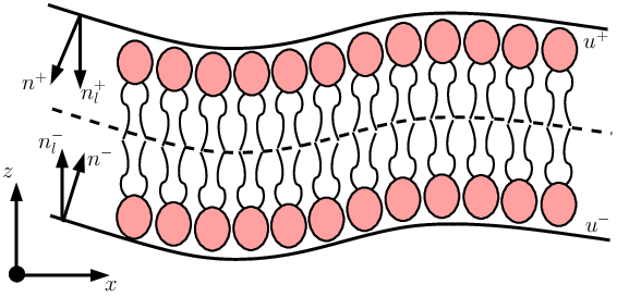
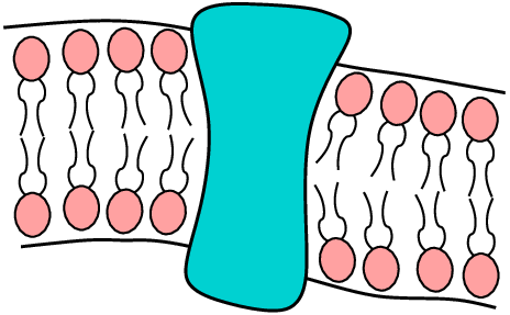
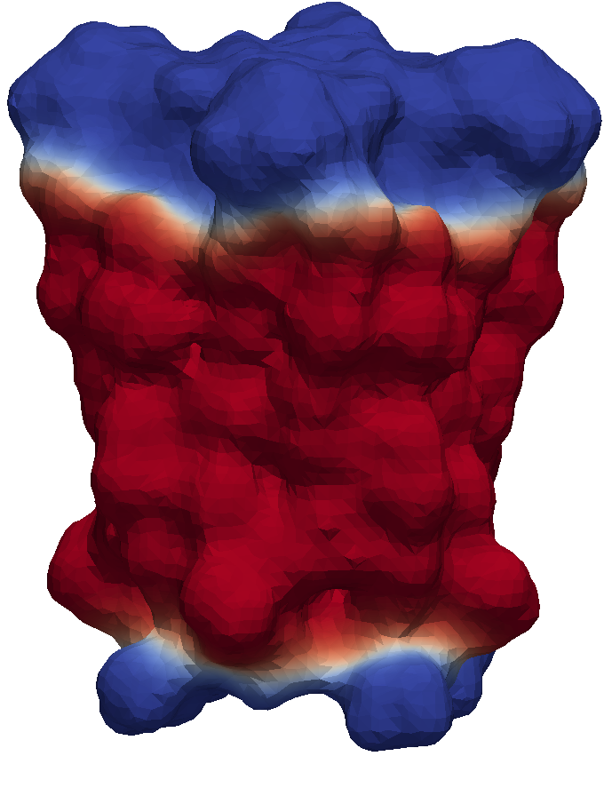
Figure 1: Illustration of protein inclusion in a lipid bilayer. Left: the two membrane surfaces and the attached vectors. Middle: The protein inclusion causes the unalignment of the lipid vectors from two bilayers near the inclusion. Right: The protein inclusion with two protein-membrane contact curves represented as the boundaries of a surface phase field function.

On the other hand, the transmembrane protein contacts with the two membrane surfaces at two closed curves, as shown in Fig. 1(right), where they are modelled as zero-level sets of the phase field function $\psi$ defined on the protein surface, with red patch being the protein surface inside the bilayer while the blue patch in the aqueous solution exterior to the bilayer.

2.1 Energetics of Solvated Protein-Membrane Complex

The total free energy $G$ for the entire protein-membrane complex is defined as the summation of the electrostatic potential energy $G^{e}$, the nonpolar energy $G^{np}$, the membrane elastic energy $G^{me}$, and the geodesic curvature energy $G^{geo}$ of protein-membrane interfaces:

$$G=G^{e}+G^{np}+G^{me}+G^{geo}.$$ (4)

Here the energy $G^{geo}$ is defined on the protein surface $\mathcal{P}$ by

$$G^{geo}=\int_{\mathcal{P}}K_{l}\left[\xi\Delta_{s}\psi+\frac{1}{2\xi}(1-\psi^{2})\psi\right]^{2}ds$$ (5)

where $\psi\in[-1,1]$ is the phase field function, $\Delta_{s}$ is the surface Laplacian, $\xi>0$ is a parameter adjusting the transition of $\psi=-1$ in the bilayer to $\psi=1$ in the aqueous solution, and $K_{l}$ is the line tension coefficient. The square bracketed function is the approximation of the geodesic curvature using the surface phase field function [22]. Here it is associated with line tension on the protein-membrane interface. The electrostatic potential energy $G^{e}$ is given by

$$G^{e}=\int_{\Omega}\left[\frac{\epsilon}{2}|\nabla\phi|^{2}-q\phi-\kappa^{2}\cosh(\phi)\right]dx,$$ (6)

where $\phi$ is the electrostatic potential, $\Omega$ is a 3-D domain containing the membrane-protein complex, $\epsilon$ is the dielectric permittivity which takes different values in different molecular domains, $q$ is the spatial-dependent charge density, $\kappa$ is the ionic strength in the solvent (and thus is zero in proteins or lipid bilayers). Our model of electrostatics can be replaced by other variational formulations of implicit solvent models to include more sophisticated dielectric effects such as nonlocal responses [37, 38, 39], finite particle size of ions and solvent [40, 41], or surface charge or dipolar densities of bilayers [7, 42]. The discontinuity of $\epsilon$ at the membrane surfaces shall induce dielectric surface forces, generating a driving force for membrane deformation.

The nonpolar energy $G^{np}$ is defined to be the work for transferring solute molecules between polar and nonpolar solvents, given by a function of the Solvent Accessible Surface Area (SASA)

$$G^{np}=\gamma_{A}(A_{m}-A_{s}),$$ (7)

where $\gamma_{A}$ is the constant characterizing the energy to transfer a unit molecular surface area from the polar to non-ploar solvent [43], and $A_{m},A_{s}$ are SASAs in the interior and exterior of the bilayer, respectively. The term proportional to the molecular volume as seen in many nonpolar solvation energy models [24, 44] is not considered here. The lateral pressure varies drastically across the bilayer because of the highly inhomogeneous molecular structure of the bilayer, and thus there does not exist a constant of proportionality similar to the uniform hydrostatic pressure in the aqueous solvent [45, 46, 47]. Microscopic chemical potentials have been defined to quantify the dependence of lateral pressure on the cross-sectional area of the protein [48, 49]. Energetically these efforts amount to relate the mechanical energy of the protein inclusion to the change of membrane morphology which will be modelled by $G^{me}$. It is therefore necessary to remove the volume term of the nonpolar solvation energy in our model to avoid double counting. With the surface phase field function $\psi$ we can conveniently approximate

$$A_{m}=\int_{\mathcal{P}}(\psi-1)ds,\quad A_{s}=-\int_{\mathcal{P}}(\psi+1)ds.$$ (8)

The membrane elastic energy $G^{me}$ includes the energies associated with the fundamental modes of membrane deformations and lipid tilt:

$$G^{me}= \int_{S}\frac{K_{c}}{2}\left[(\nabla^{2}u^{+}+\nabla\cdot t^{+}-J_{0}^{+})^{2}+(\nabla^{2}u^{-}-\nabla\cdot t^{-}-J_{0}^{-})^{2}\right]ds+$$

$$\int_{S}\frac{K_{G}}{2}\left(K^{-}+K^{+}\right)ds+\int_{S}\frac{\alpha}{2}\left(|\nabla u^{-}|^{2}+|\nabla u^{+}|^{2}\right)ds+$$

$$\int_{S}\frac{K_{\alpha}}{L_{0}^{2}}(u^{+}-u^{-})^{2}ds+\int_{S}\frac{K_{t}}{2}\left(|t^{+}|^{2}+|t^{-}|^{2}\right)ds+$$

$$\int_{S}\frac{K_{tw}}{2}\left(|\nabla\times t^{+}|^{2}+|\nabla\times t^{-}|^{2}\right)ds+\int_{S}\frac{K_{e}}{2}\left(|n^{+}-n_{0}|^{2}+|n^{-}-n_{0}|^{2}\right)ds,$$ (9)

where the integrals in order represent the splay (mean curvature), saddle splay (Gaussian curvature), surface tension, compression of membrane surfaces and tilt-stretch, tilt-twist, and configurational entropic cost of lipid chains, with respective constant coefficients $K_{c}$ the bending modulus, $K_{G}$ the Gaussian modulus, $\alpha$ the surface tension coefficient, $K_{\alpha}$ the compression modulus, $K_{t},K_{tw},K_{e}$ the moduli of tilt, tilt-twist, and configurational confinement [33]. $J_{0}^{\pm},n_{0}^{\pm}$ are the spontaneous mean curvature and spontaneous director vector of the respective surfaces. These constants are assumed to be the same for two leaflets, though their dependence on the lipid composition can be introduced at the cost of computational complexity. $G^{\pm}$ are the Gaussian curvatures of the respective monolayers. The energetic modelling of membrane deformation modes has been classical and can be reduced to the Canham-Helfrich energy density [11, 12, 13]. Lipid tilt has been recognized important recently [34, 35] and proved to be critical in describing the energy pathway of membrane fusion during which lipid directors mismatch significantly [36]. For protein inclusions with arbitrary shape we expect the lipid directors would also differ significantly from those away from the inclusion.

2.2 Variational Principles and Nonlinear PDEs for the Hybrid Model

Given the fixed 2-D domain $S$ for the Monge parameterization of the membrane surfaces, the static manifold $\mathcal{P}$ modeling the protein surface, and the fixed 3-D domain $\Omega$ containing the entire solvated protein-membrane complex, the total energy $G$ depends only on the membrane surface heights $u^{\pm}$ and the lipid directors $t^{\pm}$, noticing that the electrostatic potential $\phi$ depends on dielectric function $\epsilon$ which in turn depends on $u^{\pm}$. We shall compute the variational derivatives of $G$ with respect to $\phi,\psi$ and $u^{\pm},t^{\pm}$ to obtain the differential equations for $\phi,\psi$ and $u^{\pm},t^{\pm}$. For $\phi$ we will have the Poisson-Boltzmann equation [50, 51]

$$-\nabla\cdot(\epsilon\nabla\phi)+\kappa^{2}\sinh(\phi)=q.$$ (10)

For $\psi$ we first compute

$$g(\psi)=\frac{\delta G}{\delta\psi}=\frac{\delta G^{geo}}{\delta\psi}+\frac{\delta G^{np}}{\delta\psi}=\Delta_{s}W-\frac{1}{\xi^{2}}(3\psi^{2}-1)W+2\gamma_{A},$$ (11)

where

$$W=\xi\Delta_{s}\psi+\frac{1}{\xi}(1-\psi^{2}).$$ (12)

The evolution of the protein-membrane contact curves along the pseudo-time $t$ will follow the weak gradient flow of $\psi$:

$$\frac{\partial\psi}{\partial t}=-\frac{\delta G}{\delta\psi}=\Delta_{s}W_{L}+\frac{1}{\xi^{2}}W_{L}+\Delta_{s}W_{N}-\frac{3}{\xi^{2}}\psi^{2}W+\frac{1}{\xi^{2}}W_{N}-2\gamma_{A},$$ (13)

where

$$W_{L}=\xi\Delta_{s}\psi+\frac{1}{\xi}\psi,\quad W_{N}=-\frac{1}{\xi}\psi^{3}$$ (14)

are respectively the linear and nonlinear components of $W$ such that $W=W_{L}+W_{N}$. This splitting will facilitate the numerical treatment of the Allan-Cahn equation (13). Here the phase boundary is tracked without enforcing the total quantity of either phase, thus our model is free of the conservation constraints and the associated Lagrangian multipliers [52, 22]. Our approach here is different from those based on the geodesic active contours [53, 54], where an Euler-Lagrange equation is first derived for minimizing the curve energy in sharp interface formulation and then approximated using a level set form [27, 30],

To derive the Euler-Lagrange equations for the unknowns $u^{\pm},t^{\pm}$ we recognize that the dielectric function $\epsilon$ also depends on $u^{\pm}$, thus we shall also consider the variational derivative of $G^{e}$ with respect to $u^{\pm}$. This derivative, by definition, is identical to the shape derivative of the electrostatic potential energy under the smooth velocity field induced by the displacement $u^{\pm}$ [42], and thus gives the electrostatic forces $f_{e}$ on the membrane surfaces:

$$f^{\pm}_{e}=-\frac{\epsilon_{s}}{2}|\nabla\phi^{\pm}_{s}|^{2}+\frac{\epsilon_{m}}{2}|\nabla\phi_{m}^{\pm}|^{2}+\epsilon_{m}(\nabla\phi_{s}^{\pm}\cdot n^{\pm})(\nabla\phi_{m}^{\pm}\cdot n^{\pm})-\cosh(\phi),$$ (15)

where $\phi_{s},\phi_{m}$ are respectively the electrostatic potentials on the solution and membrane sides. The Euler-Lagrange equations for $u^{-},t^{-}$ shall read

$$K_{c}\Delta(\Delta u^{-}-\nabla\cdot t^{-}+J_{0}^{-})-K_{e}\nabla\cdot(\nabla u^{-}-t^{-}+n_{0}^{-})-\alpha\Delta u^{-}+2\frac{K_{\alpha}}{L_{0}^{2}}(u^{-}-u^{+}) =f_{e}^{-},$$ (16)

$$(K_{t}+K_{e})t^{-}-K_{e}(\nabla u^{-}+n_{0})+K_{c}\nabla(\Delta u^{-}-\nabla\cdot t^{-}+J_{0}) =0,$$ (17)

noticing that $\epsilon$ does not depend on $t^{-}$ so the variational derivatives of $G^{e}$ do not generate a forcing term for $t^{-}$. Equations for $u^{+},t^{+}$ can be obtained similarly. The coupling of $u$ with $t$ in these equations motivates us to think of approaches to decouple them to facilitate numerical treatment. The assumption of infinite two-dimensional wall on the surface of protein inclusion as put forward by May et. al. [55, 56] is not applicable to our modeling of the protein-membrane complex because it contradicts our consideration of the realistic protein geometry. Instead, we assume that only within a lipid tail length the values of $K_{e}$ and $n_{0}$ are constants equaling to the values right at the protein-membrane interface in May’s model [56]. Beyond that length different constants are taken, leading to the following piecewise definition of the two constants:

$$\frac{K_{e}}{k_{B}T}=\frac{12}{A_{0}},\quad n_{0}=-\frac{1}{2}n_{p}, 0\leq r\leq h_{0},$$ (18)

$$\frac{K_{e}}{k_{B}T}=\frac{3}{A_{0}},\quad n_{0}=0, r>h_{0},$$ (19)

where $n_{p}$ is the unit binormal vector on the protein-membrane contact curves, $r$ is distance in the normal direction away from the protein surface, and $A_{0}$ is the cross-sectional area of each lipid chain. Consequently, one can remove $J_{0}^{-},n_{0}^{-}$ from Equation (16) and take divergence of Equation (17) to get

$$K_{c}\Delta(\Delta u^{-}-\nabla\cdot t^{-})-K_{e}\nabla\cdot(\nabla u^{-}-t^{-})-\alpha\Delta u^{-}+2\frac{K_{\alpha}}{L_{0}^{2}}(u^{-}-u^{+}) =-f_{e}^{-},$$ (20)

$$(K_{t}+K_{e})\nabla\cdot t^{-}-K_{e}\Delta u^{-}+K_{c}\Delta(\Delta u^{-}-\nabla\cdot t^{-}) =0.$$ (21)

We observe in Equations (20,21) that

$$K_{e}\nabla\cdot(\nabla u^{-}-t^{-})+\alpha\Delta u^{-}-2\frac{K_{\alpha}}{L_{0}^{2}}(u^{-}-u^{+})-f_{e}^{-}=-(K_{t}+K_{e})\nabla\cdot t^{-}+K_{e}\Delta u^{-},$$ (22)

and thus we can solve for $\nabla\cdot t^{-}$:

$$\nabla\cdot t^{-}=-\frac{\alpha}{K_{t}}\Delta u^{-}+\frac{2K_{\alpha}}{K_{t}L_{0}^{2}}(u^{-}-u^{+})+\frac{f_{e}^{-}}{K_{t}}.$$ (23)

Put this back to Equation (16) we will get

$$\Delta^{2}u^{-}-\chi^{-}\Delta(u^{-}-u^{+})-\gamma^{-}\Delta u^{-}+\beta^{-}(u^{-}-u^{+})=\hat{f}_{e}^{-},$$ (24)

with

$$\chi^{-}=\frac{2K_{\alpha}}{L_{0}^{2}(K_{t}+\alpha)},\quad\gamma^{-}=\frac{K_{e}}{K_{c}}+\frac{K_{t}\alpha}{K_{c}(K_{t}+\alpha)},\quad\beta^{-}=\frac{2K_{\alpha}}{L_{0}^{2}K_{c}}\frac{K_{t}+K_{e}}{K_{t}+\alpha},$$

and

$$\hat{f}_{e}^{-}=\frac{K_{c}\Delta f_{e}^{-}-(K_{t}+K_{e})f_{e}^{-}}{K_{c}(K_{t}+\alpha)}.$$

A similar equation for $u^{+}$ shall read

$$\Delta^{2}u^{+}-\chi^{+}\Delta(u^{-}-u^{+})-\gamma^{+}\Delta u^{+}+\beta^{+}(u^{-}-u^{+})=\hat{f}_{e}^{+},$$ (25)

with

$$\chi^{+}=\frac{-2K_{\alpha}}{L_{0}^{2}(K_{t}-\alpha)},\quad\gamma^{+}=\frac{K_{e}}{K_{c}}+\frac{K_{t}\alpha}{K_{c}(K_{t}-\alpha)},\quad\beta^{+}=\frac{2K_{\alpha}}{L_{0}^{2}K_{c}}\frac{K_{t}-K_{e}}{K_{t}-\alpha},$$

and

$$\hat{f}_{e}^{+}=-\frac{K_{c}\Delta f_{e}^{+}-(K_{t}-K_{e})f_{e}^{+}}{K_{c}(K_{t}-\alpha)}.$$

Proper boundary conditions are needed for the solutions of equations we derived above. Electrostatic potential induced by fixed charges of the protein in the aqueous solution where $\epsilon_{w}\approx 80$ can be used as the approximate boundary conditions of the Poisson-Boltzmann equation (10) on $\partial\Omega$ [57, 58]. The surface Allan-Cahn equation does not need a boundary condition as it is defined on the closed protein surface $\mathcal{P}$. For the coupled fourth-order equations (24,25) we adopt the fixed boundary condition (homogeneous Dirichlet boundary condition for biharmonic equations) on the boundary far away from the protein inclusion:

$$u^{\pm}=0,\quad\nabla u^{\pm}\cdot n=0,$$ (26)

indicating that the membrane is free of deformation on $\partial\Omega$. The protein-membrane interfaces are indeed the contact curves of three phases: the aqueous solvent, the protein, and the bilayer. Wang et. al. [31] proposed a modification of the classical Young’s contact angle [32] to include the tension energy of the contact line among solid-liquid-vapor phases:

$$\gamma_{lv}\cos\theta=\gamma_{sl}-\gamma_{sv}+\frac{\tau}{R}$$ (27)

where $\theta$ is the $\gamma_{lv},\gamma_{sl},\gamma_{sv}$ are respectively the surface tensions of liquid-vapor, solid-liquid, and solid-vapor interfaces, $\tau$ is the line tension and $R$ is the radius of the base of the liquid drop in contact with the solid. It is interesting to recognize that if the base contact curve is a geodesic then $1/R$ shall be zero and the classical Young’s contact angle is reproduced. Therefore at our protein-water-lipid interface we will have

$$\cos\theta=\frac{\gamma_{pl}}{\gamma_{lw}}-\frac{\gamma_{pw}}{\gamma_{lw}}.$$ (28)

The protein-water interface tension was well-estimated [59], and given the fluidity of the lipid molecules in the two-dimensional surface we postulate that $\gamma_{pl}\approx\gamma_{pw}$ thus $\cos\theta=0$, leading to an estimate that $\theta=\pi/2$. This suggests that the two membrane surfaces are locally orthogonal to the protein surface at the protein-membrane contact curves, thus the following fixed boundary conditions will be adopted

$$u^{\pm}=u_{B}^{\pm},\quad\nabla u^{\pm}\cdot n=\theta_{p},$$ (29)

where $u_{B}^{\pm}$ are the positions of the protein-membrane contact curves and $\theta_{p}$ is the projection of the unit normal direction at the contact curves onto the common $x-y$ base plane on which the Monge parameterizations of the two membrane surfaces are defined.

3 Numerical Techniques for the Nonlinear PDEs

In this section we discuss the numerical solutions of the differential equations and the convergent iterations for their coupling. The evolving protein-membrane contact curves on the protein surfaces present varying dielectric interface for the Poisson-Boltzmann equation, so a numerical method that does not require the regeneration of interface conforming 3-D mesh is preferred. Here we adopt a tree-code accelerated boundary integral method for solving the Poisson-Boltzmann equation [60, 61]. The molecular surface mesh of the protein-membrane complex will be updated when the protein-membrane contact curves evolve or the membrane surfaces are deformed with the given contact curves.

Our numerical treatments of the problem are focused on the solutions of the surface Allan-Cahn equation (13), the surface deformation equations (24,25), and their convergent coupling with the Poisson-Boltzmann equation. The $C^{0}$ interior penalty discontinuous Galerkin (DG) method [62, 22] is not applicable to the surface deformation equations as they only admit Cahn-Hilliard type boundary conditions while we have the Dirichlet boundary conditions here. Based on the DG method in [63] we develop an alternative $C^{0}$ interior penalty method to solve the deformation equations (24,25). Consider the following prototype of the surface deformation equation with Dirichlet boundary conditions $(g_{D},g_{N})$:

$$\Delta^{2}u+\beta_{1}\Delta u+\beta_{2}u=f,\quad u=g_{D},~{}\nabla u\cdot n=g_{N},$$ (30)

on the annulus domain $\mathcal{R}$, c.f. Fig. 6(right). Let $\mathcal{T}_{h}$ be a regular simplifical triangulation of $\mathcal{R}$. We will use the following standard notions for defining discontinuous Galerkin methods:

• $h_{T}$: diameter of the triangle $T\in\mathcal{T}_{h}$, where $h=\max_{T\in\mathcal{T}_{h}}h_{T}$,

• $\mathcal{E}_{h}$: set of edges of the triangles in $\mathcal{T}$,

• $\mathcal{E}_{h}^{i}$: subset of $\mathcal{E}_{h}$ consisting of edges interior to $\mathcal{R}$,

• $\mathcal{E}_{h}^{b}$: subset of $\mathcal{E}_{h}$ consisting of edges on the boundary $\partial\mathcal{R}$,

• $|T|,|e|$: the area of the triangle $T$, and the length of the edge $e$.

On an interior edge $e$ that is shared by the two triangles $T_{\pm}$ we define the normal vector $n_{e}$ pointing from $T_{-}$ to $T_{+}$ and the jump and average quantities:

$$\llbracket v\rrbracket=u_{+}-u_{-},\qquad\{\mskip-5.0mu\{u\}\mskip-5.0mu\}=\frac{1}{2}(u_{+}+u_{-})$$

for $u\in H^{1}(\mathcal{R},\mathcal{T}_{h})$. Here the subscripts $\pm$ signify the limit values of the function at the common edge $e$ on the triangles $T_{\pm}$. These definitions are extended to the boundary edge $e\in\mathcal{E}^{b}_{h}$ where

$$\llbracket v\rrbracket=\{\mskip-5.0mu\{u\}\mskip-5.0mu\}=u|_{e}.$$

We associate with $\mathcal{T}_{h}$ a standard quadratic Lagrange finite element space $V_{h}=\{v\in C(\bar{\mathcal{R}}):v_{T}=v|_{T}\in P_{2}(T),\forall T\in\mathcal{T}_{h}\}$. The approximate solution $u_{h}\in V_{h}$ to Equation (30) is given by

$$\mathcal{B}(u_{h},v_{h})=l(v_{h}),\quad\forall~{}v_{h}\in V_{h},$$ (31)

where the bilinear form $\mathcal{B}(\cdot,\cdot)$ and the linear functional $l(\cdot)$ are given, respectively, by

$$\mathcal{B}(u_{h},v_{h})= \sum_{T\in\mathcal{T}_{h}}\int_{T}\big{(}\Delta u_{h}\Delta v_{h}+\beta_{1}\nabla u_{h}\cdot\nabla v_{h}+\beta_{2}u_{h}v_{h}\big{)}dx+$$

$$+ \sum_{e\in\mathcal{E}^{b}_{h}}\int_{e}\alpha_{1}u_{h}v_{h}ds$$

$$+ \sum_{e\in\mathcal{E}_{h}}\int_{e}\left(-\left\llbracket\frac{\partial u_{h}}{\partial n_{e}}\right\rrbracket\{\mskip-5.0mu\{\Delta v_{h}\}\mskip-5.0mu\}-\left\llbracket\frac{\partial v}{\partial n_{e}}\right\rrbracket+\alpha_{2}\left\llbracket\frac{\partial u_{h}}{\partial n_{e}}\right\rrbracket\left\llbracket\frac{\partial v_{h}}{\partial n_{e}}\right\rrbracket\right)ds,$$ (32)

$$l(v_{h})= \sum_{T\in\mathcal{T}_{h}}\int_{T}fv_{h}dx+\sum_{e\in\mathcal{E}_{h}^{b}}\int_{e}\left(-g_{N}\Delta v_{h}+\alpha_{1}g_{D}v_{h}+\beta_{1}g_{N}\frac{\partial v_{h}}{\partial n_{e}}\right)ds.$$ (33)

Here the penalty parameters $\alpha_{1},\alpha_{2}$ are given by

$$\alpha_{1}=C_{1}h^{-3},\quad\alpha_{2}=C_{2}h^{-1}$$ (34)

for sufficiently large positive constants $C_{1},C_{2}$ that depend only on the triangulation $\mathcal{T}_{h}$. The optimal convergence of this interior penalty DG method and the generalization of the analysis to higher order basis functions are given in [63].

Coupling of the deformation of two membrane surfaces demands the two equations (24,25) to be defined on the same domain. However, this appears not the case because of the different contact curves of the transmembrane protein with two membrane surfaces. Since the two surfaces are expected to match point-wisely we are motivated to define smooth mapping between the middle plane and the base planes of two membrane surfaces. We define the interior boundary of the middle plane as a circle whose radius and height are the respective average radius and height of the two contact curves. The exterior boundary is at the middle of the exterior boundaries of the two surfaces. These mappings are numerically established by solving two Winslow equations [64] on the annulus domain $\mathcal{R}$ in the middle plane. The meshes are locally refined toward the contact curves where larger membrane deformations are expected, c.f. Fig. 6(right).

Approximation of the surface biharmonic and surface Laplacian for the solution of Equation (13) can be done as in (32,33), without terms related to the boundary conditions though, as the evolution of phase field function is on a closed 2-manifold $\mathcal{P}$ approximated by a simplicial surface triangulation. There are many energy stable time discretization schemes developed for the phase-field models, including convex splitting methods [65, 66, 67], exponential time discretization schemes [68], IEQ schemes [69], and semi-implicit methods [70]. Many of these methods introduce a chemical potential as an intermediate variable to reduce the fourth-order Allan-Cahn or Cahn-Hilliard equation to two coupled second-order equations, which is not consistent with our discontinuous Galerkin approximation. Here the implicit method we developed for the surface Allan-Cahn equation [22] will be adapted. The method begins with a Crank-Nicolson approximation of the time derivation in Equation (13), giving rise to

$$\frac{\psi_{n+1}-\psi_{n}}{\Delta t}+g(\psi_{n+1},\psi_{n})+2\gamma_{A}=0,$$ (35)

where $\Delta t$ is the time increment. The average function $g(\psi_{n+1},\psi_{n})$ is defined as

$$g(\psi_{n+1},\psi_{n})= \frac{1}{2}\Delta_{s}\left(f_{c}(\psi_{n+1})+f_{c}(\psi_{n})\right)$$

$$- \frac{1}{2\xi^{2}}\left(\psi^{2}_{n+1}+\psi_{n+1}\psi_{n}+\psi_{n}^{2}-1)\big{(}f_{c}(\psi_{n+1})+f_{c}(\psi_{n})\big{)}\right)$$ (36)

with

$$f_{c}(\psi)=\xi\Delta_{s}\psi+\frac{1}{\xi^{2}}(1-\psi^{2}).$$

To solve Equation (35) which is nonlinear and implicit in $\psi_{n+1}$, we define inner iterations on the variable $\Psi_{m}$ which is expected to converge to $\psi_{n+1}$ as $m\rightarrow\infty$. Replacing all linear and nonlinear terms of $\psi_{n+1}$ respectively using $\Psi_{m+1}$ and $\Psi_{m}$, we can get the following inner iteration

$$\frac{\Psi_{m+1}-\psi_{n}}{\Delta t}+g(\psi_{n},\Psi_{m},\Psi_{m+1})+2\gamma_{A}=0,$$ (37)

with the new average function

$$g(\psi_{n},\psi_{n},\Psi_{m+1})= \frac{1}{2}\Delta_{s}\tilde{f}_{c}(\psi_{n},\Psi_{m},\Psi_{m+1})-\frac{1}{2\xi^{2}}\left(\Psi_{m}^{2}+\Psi_{m}\psi_{n}+\psi_{n}^{2}-1)(f(\Psi_{m})+f(\psi_{n})\right)$$ (38)

where

$$\tilde{f}_{c}(\psi_{n},\Psi_{m},\Psi_{m+1})=\frac{\xi}{2}\Delta_{s}(\Psi_{m+1}+\psi_{n})-\frac{1}{4\xi}(\Psi_{m}+\psi_{n}^{2}-2)(\Psi_{m}+\psi_{n}).$$

Now the equation (37) is linear in $\Psi_{m+1}$ as we expect:

$$\left(1+\frac{\xi\Delta t}{2}\Delta_{s}^{2}\right)\Psi_{m+1}= \psi_{n}-\frac{\xi\Delta t}{2}\Delta_{s}^{2}\psi_{n}+\frac{\Delta t}{4\xi}\Delta_{s}(\Psi_{m}^{2}+\psi_{n}^{2}-2)(\Psi_{m}+\psi_{n})$$

$$+ \frac{\Delta t}{2\xi^{2}}\Delta_{s}(\Psi_{m}^{2}+\Psi_{m}\psi_{n}+\psi_{n}^{2})\left(f_{c}(\Psi_{m})+f_{c}(\psi_{n})\right)+2\Delta t\gamma_{A}.$$ (39)

Since the surface phase field model can only find the local minimum of the geodesic curvature energy, we will scan a range of initial protein-membrane contact curves to finally find the global minimum of the total energy $G$ defined in Equation (4). The full algorithm of our energetic model is summarized below:

Algorithm 3.1.

1. Define a proper range for the initial position of bilayer with respect to the given membrane protein. Divide the range into small intervals for the loop in Step 2 below.

2. For each initial position of the bilayer:

   1. Update the protein-membrane interfaces by solving the surface phase field equation (39).

   2. Update the mappings from the middle plane to the base planes of two membrane surfaces.

   3. Update the electrostatic surface forces by solving the Poisson-Boltzmann equation with updated membrane surfaces.

   4. Update the membrane surfaces by solving the coupled surface deformation equations.

   5. Return to Step (ii) until convergence. Save total energy $G$.

3. Choose the minimum $G$ and the corresponding geometry of protein-membrane complex.

4 Model Validation and Computational Simulations

In this section we shall first validate our geodesic curvature modelling of the protein-membrane interfaces. We will then present examples of mapping the base planes of membrane surfaces to the middle annulus. We will finally apply these validated modules of our energetic model for the determination of inclusion state of the transmembrane protein.

4.1 Validation of geodesic curvature model

We first apply our geodesic curvature model to capture the curve on a molecular surface with the well-identified local minimal geodesic curvature. The molecule mimics the carbon backbone of a benzene ring with six atoms in $y$-plane of unit radius respectively centered at $(x,z)=(2.5,0)$, $(1.25,2.165)$,
$(-1.25,2.165)$, $(-2.5,0)$, $(-1.25,-2.165)$ and $(1.25,-2.165)$. In the first test, shown in Fig. 2, we chose the initial phase field $\phi=1$ for $z_{ini}\in[-1.62,1.52]$ and $\phi=-1$ elsewhere. This asymmetrical initial condition allows the two initial phase boundaries to evolve toward local minima of different topology. The upper phase boundary evolves downward, quickly splitting into two closed curves each of which evolves toward its own local minimum of geodesic curvature energy. The lower phase boundary below, in contrast, is able to maintain its topology and evolves upward gradually settle on a local minimum. The initial position $z_{ini}=1.52$ for the upper phase boundary is near the critical point. An initial phase boundary above this critical $z$-position will not split during the evolution but converges to a final position symmetrical to the convergent position of the phase boundary initialized at $z_{ini}=-1.62$ below.

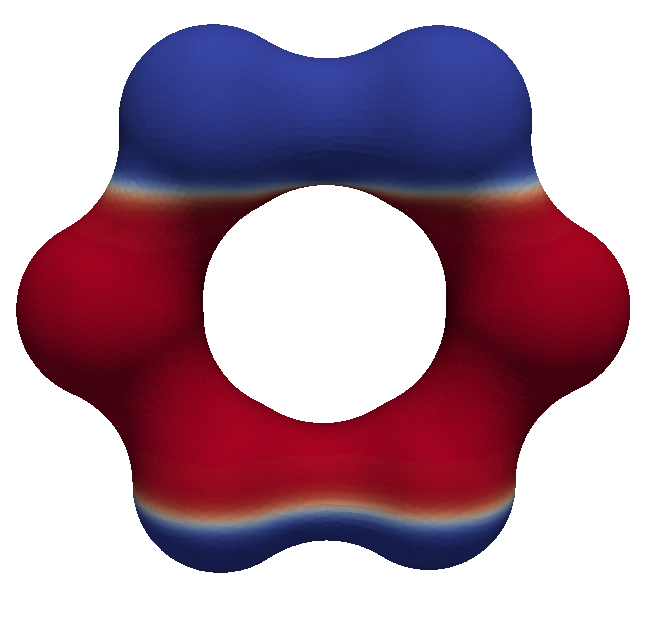
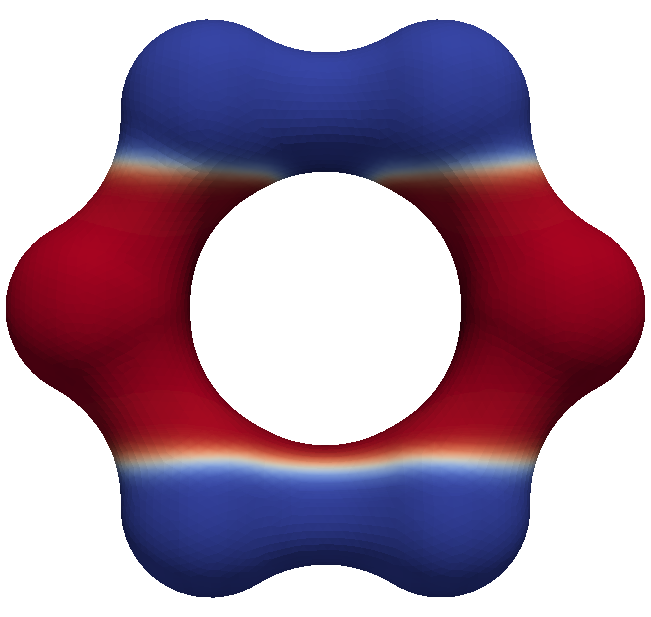
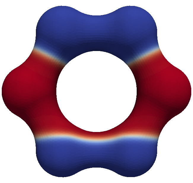
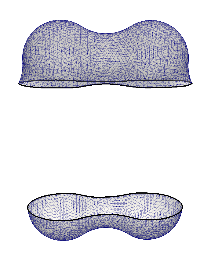
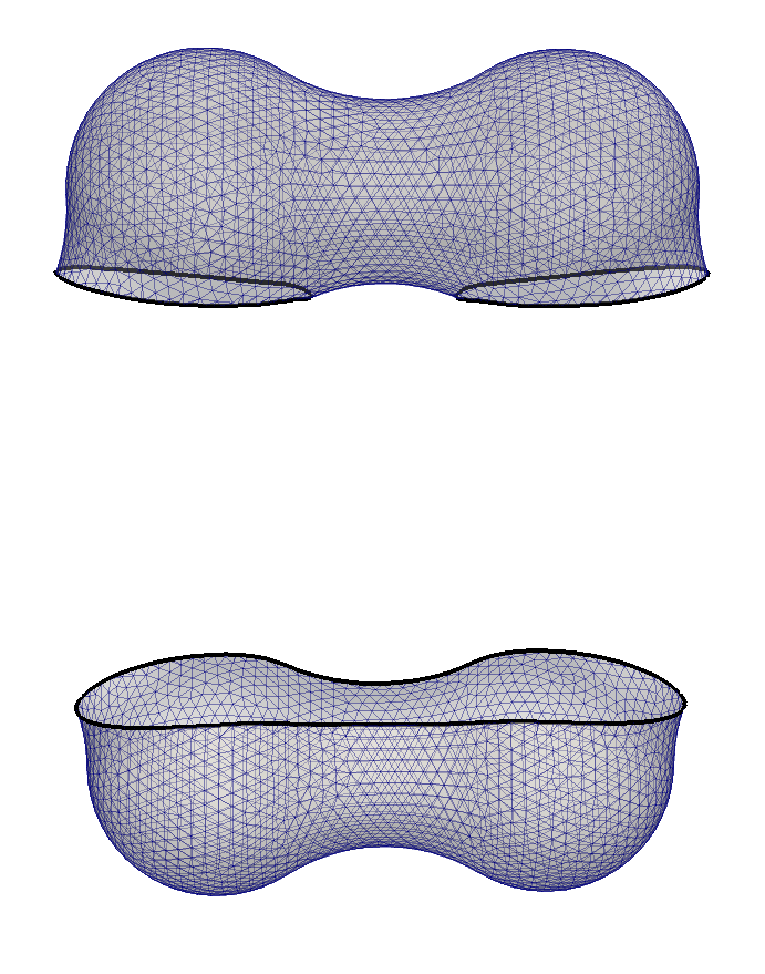
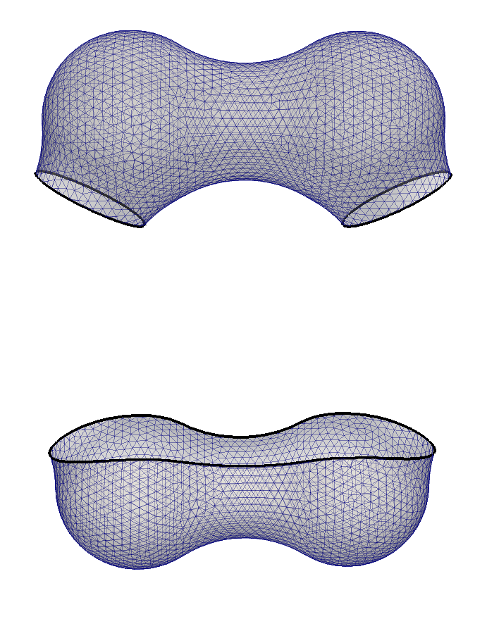
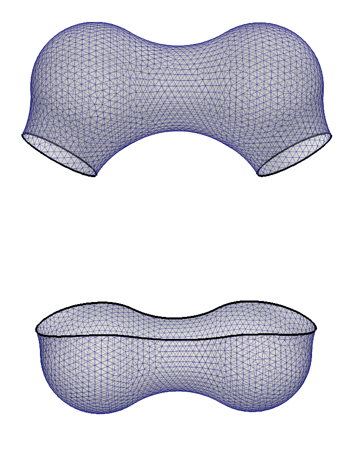
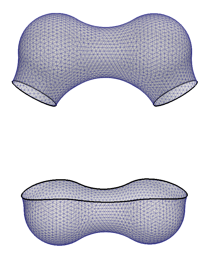
Figure 2: Snapshots in the surface phase boundary evolution on the model benzene ring at time $t=0,0.1,5,12,18$. Surface triangular mesh is quasi-uniform with $8124$ vertices and $16248$ triangles. Time increment $\Delta t=0.01$, $\xi=0.1$. Top: Plots of surface phase field function. Bottom: Surface mesh for the phase $\psi=-1$ highlights the phase boundaries with different history of topological change during the phase boundary evolution.

In the second test, shown in Fig. 3, the surface phase field is initialized with phase boundaries at $z_{ini}=-2.22$ and $0.2$, respectively. The upper phase boundary evolves upward and converges to the same local minimum found by the upper phase boundary in Fig. 2. The lower phase boundary, which is initially $0.6$ below the lower phase boundary in the first test, evolves downward, shrinks and finally disappears, achieving a local minimum geodesic curvature energy of zero.

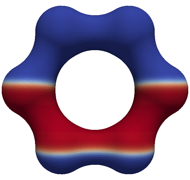
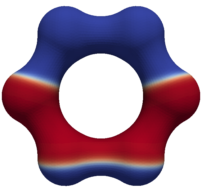
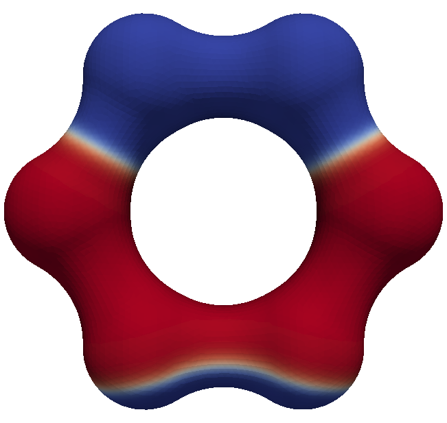
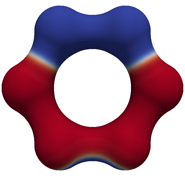
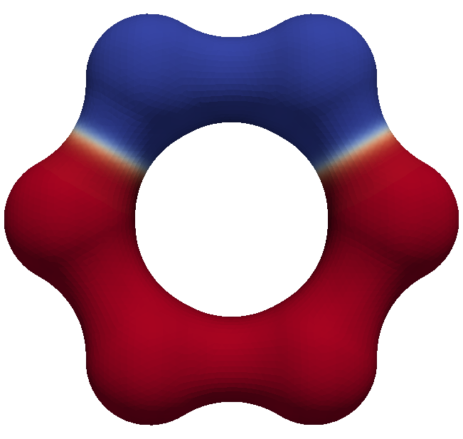
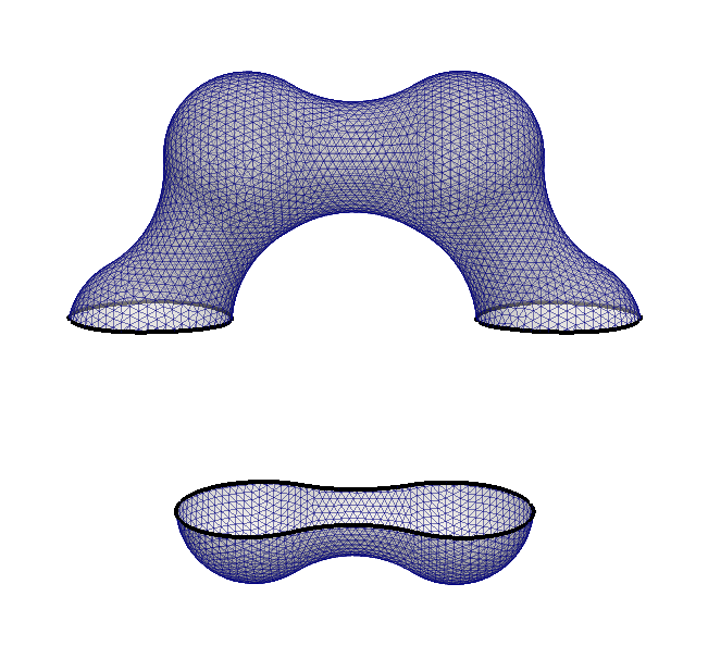
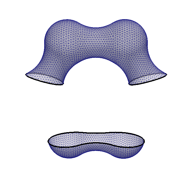
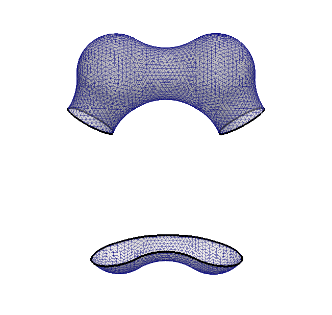
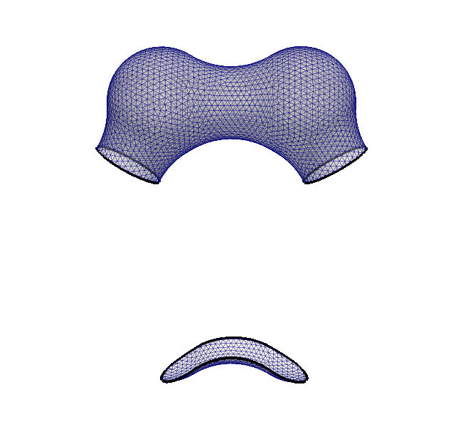
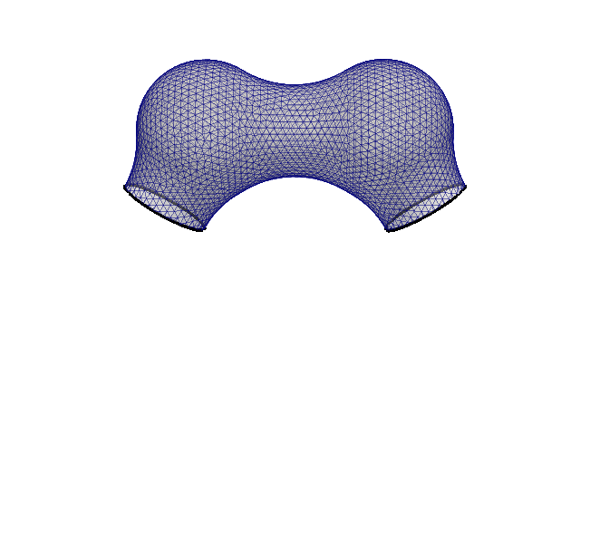
Figure 3: Snapshots in the surface phase boundary evolution on the model benzene ring at time $t=0,6,14,18,26$. Mesh and parameters are identical to the case in Fig. 2. Top: Plots of surface phase field function. Bottom: Surface mesh for the phase $\psi=-1$ highlights the phase boundaries with different history of topological change during the phase boundary evolution. The lower phase boundary disappears finally as a result of geodesic curvature minimization.

The third and fourth tests are carried out on the proton channel M2 (PDB ID: 2kqt). With a total of $3247$ atoms this protein has a rich surface morphology with many local minima of total geodesic curvature. Fig. 4 shows the evolution of the two phase boundaries initially located at $z=-10,13$. The upper phase boundary moves up considerably to the local minimum, while the lower phase boundary finds the local minimum geodesic energy after a slight adjustment of position. When the initial phase boundaries are changed to be at $z=-13,11$, shown in Fig. 5, final phase boundaries different from the third test are observed.

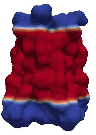
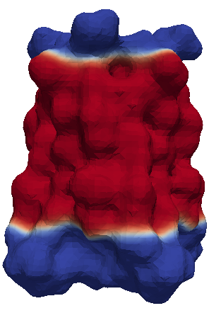
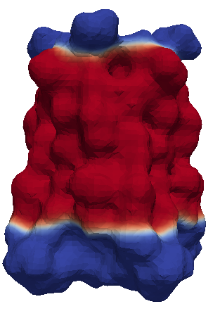
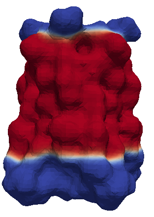
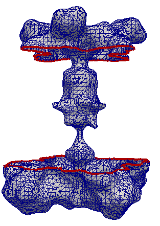
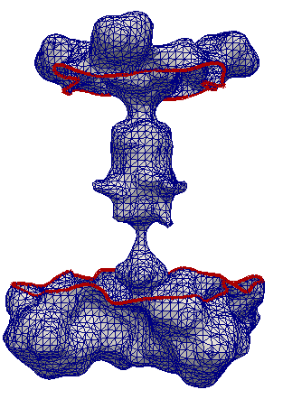
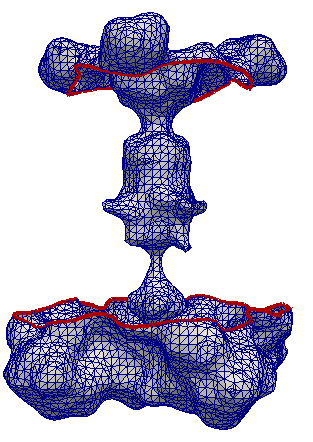
Figure 4: Snapshots in the surface phase boundary evolution on the proton channel protein (PDB ID: 2kqt) at time $t=0,20,40,60,80$. Initial phase boundaries are at $z=-10,13$. Surface triangular mesh is quasi-uniform with $12470$ vertices and $24940$ triangles. Time increment $\Delta t=0.01$, $\xi=0.5$. Left: Plots of surface phase field function. Right: Surface mesh for the phase $\psi=-1$ highlights the evolution of the phase boundaries. The pole in the center represents the open proton channel.

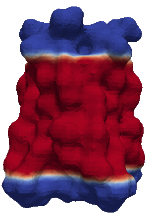
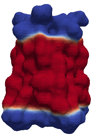
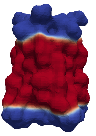
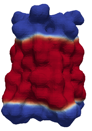
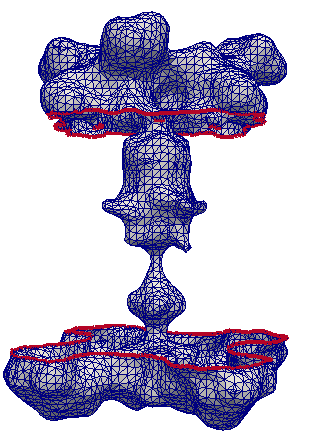
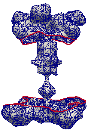
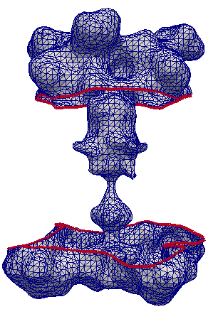
Figure 5: Snapshots in the surface phase boundary evolution on the proton channel protein (PDB ID: 2kqt) at time $t=0,20,40,60,80$. Initial phase boundaries are at $z=-13,11$. Mesh and parameters are identical to the case in Fig. 4. Left: Plots of surface phase field function. Right: Surface mesh for the phase $\psi=-1$ highlights the evolution of the phase boundaries.

These four numerical examples illustrate that our model and numerical methods are very effective in capturing the initial condition-dependent local minimum of the geodesic curvature energy. In the applications to be presented in (4.3), we will scan over the full height of the membrane protein to set a range of initial phase boundaries and to locate the global minimum from the set of local minima.

4.2 Validation of mappings to the middle plane

We consider a model transmembrane protein and two phase boundaries on its surface modeling the protein-membrane interfaces, c.f. Fig. 6 (left). The common middle annulus is defined as follows. First, the geometrical centers and radii of the upper and lower phase boundaries are found. These define the position of the base planes for the two membrane surfaces. The average radii and average height ($z$-coordinate) will be used as the inner radius of middle annulus and its $z$-coordinate. This middle annulus is then discretized on the polar coordinate, with its uniformly discretized inner circle mapped to quasi-uniformly discretized upper and lower phase boundaries. Together with the mapping between the discretized exterior circles, we have the boundaries of the two base planes mapped to the middle annulus.

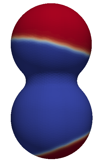
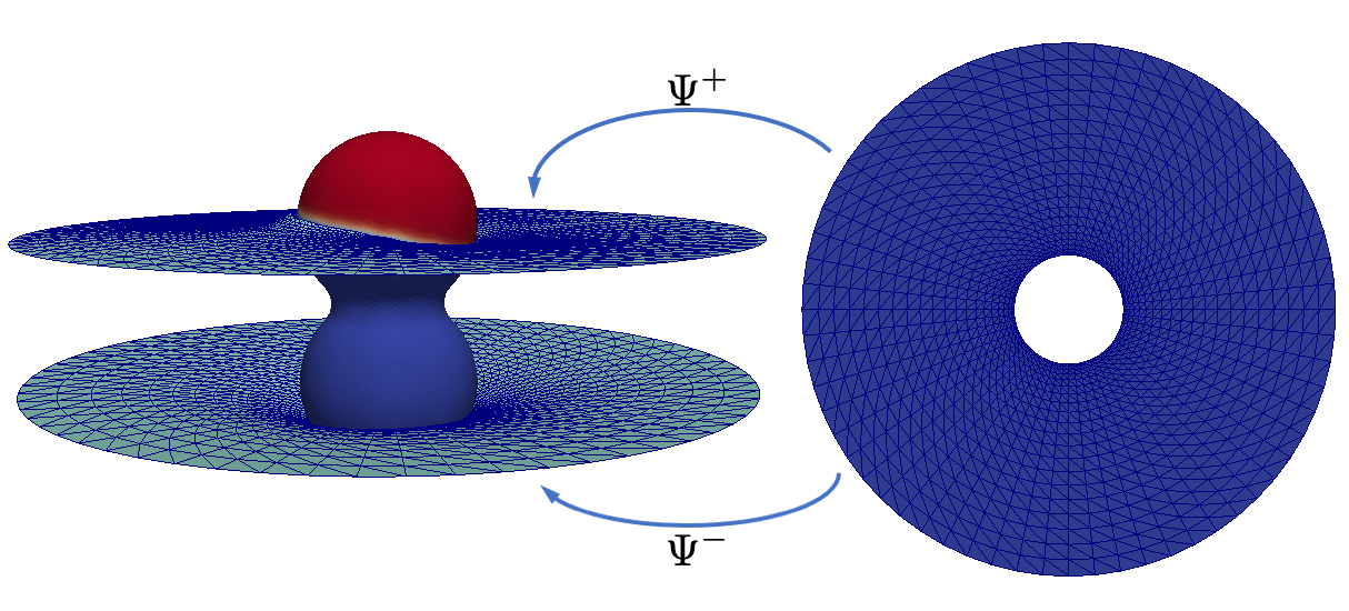
Figure 6: Illustration of membrane surfaces mapped to the same middle annulus. Left: A model protein with two surface phase boundaries representing the two contact curves with membrane surfaces. Right: The model protein is embedded in the bilayer represented as two membrane surfaces, whose Monge parameterizations are defined on the planes mapped from the same annulus $\mathcal{R}$ via respective transformations $\Psi^{\pm}$.

Inhomogeneous Thompson-Thames-Mastin elliptic grid generator ([64], Page 98) is adopted to produce interior mesh grids for the two base planes that are dense near the protein-membrane interfaces, c.f. Fig. 6 (right). The quadrilateral grid meshes are then triangulated for the solution of Eq.(24,25) using the interior penalty discontinuous Galerkin method described above. The vertices of the triangulated meshes for the two membrane surfaces inherit the one-one correspondence established on the mesh grids, allowing us to compute the coupling terms $(u^{-}-u^{+})$ and $\Delta(u^{-}-u^{+})$ in the two surface deformation equations. It is worth noting that by using the numerical mappings we do not change the physical domains or coordinate systems of the two membrane surfaces. The mappings are introduced merely to establish a one-one correspondence between the two membrane surfaces. Therefore one does not need to transform the surface deformation equations because of these numerical mappings of the computational domains.

4.3 Membrane morphology induced by protein inclusion

After validating the evolution of surface phase field function and the mapping to the middle annulus, we are now at a position to apply these methodologies on the determination of membrane morphology induced by protein inclusion. We consider a single M2 protein embedded in a homogeneous phosphatidylcholine (POPC) bilayer with equilibrium thickness $L_{0}=26\textup{\AA}$. Although the height of protein is comparable to the bilayer thickness we will still expect a considerable compression of the bilayer in the vicinity of protein inclusion because the protein-membrane interfaces are highly curved. The mechanics and dielectric parameters of the POPC bilayer are taken from [10]. The outer radius of the middle common annulus is $100\textup{\AA}$. The inner radius is about $12$ to $15\textup{\AA}$, depending on the position of the protein-membrane interfaces. The values of other parameters are $K_{c}=10.8,K_{G}=-9.8,\alpha=0.004,K_{\alpha}=0.33,k_{t}=\alpha$, all in the unit of $kcal/mol$.

We first look at the protein-membrane interfaces modelled as the phase boundaries with different surface phase field initializations $z_{ini}=\pm 8\sim\pm 14\textup{\AA}$. As shown in Fig. 7,

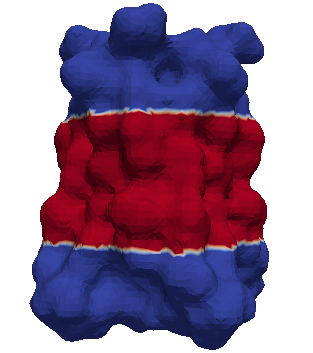
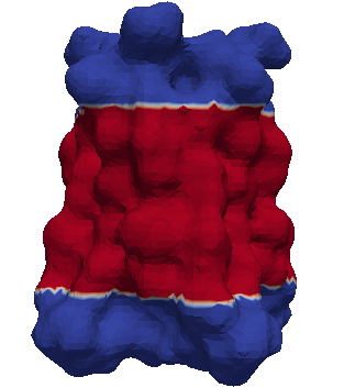
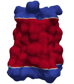
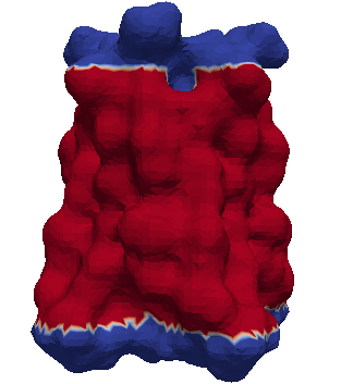
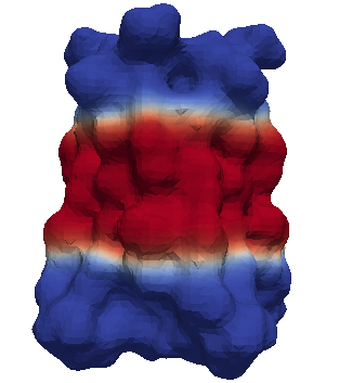
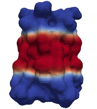
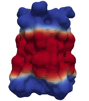
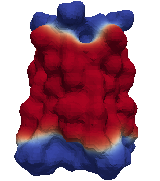
Figure 7: Surface phase fields with different initial phase boundaries (top) and the corresponding equilibrium fields (bottom). From left to right: $z_{ini}=\pm 8,\pm 10,\pm 12,\pm 14\textup{\AA}$.

the top phase boundary does not change when the initial position is placed at $8\leq z_{ini}\leq 12.5\textup{\AA}$ as they will be trapped to the same position with a local minimum geodesic curvature energy is observed. The bottom interface stays at the same local minimum for $-11.3\leq z_{ini}\leq-8\textup{\AA}$, and then moves to another local minimum for a lower initial phase boundary. We will consider these initial protein-membrane interfaces and apply Algorithm 3.1 to find the equilibrium membrane surfaces with minimum total energy, and the results are shown in Fig. 8.

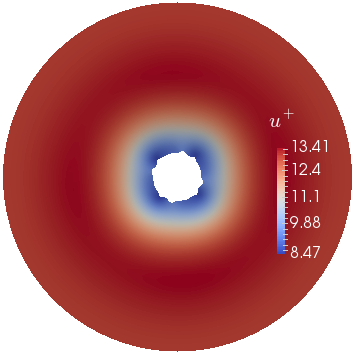
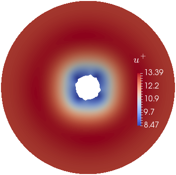
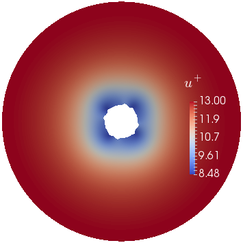
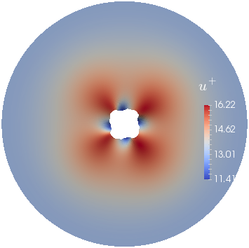
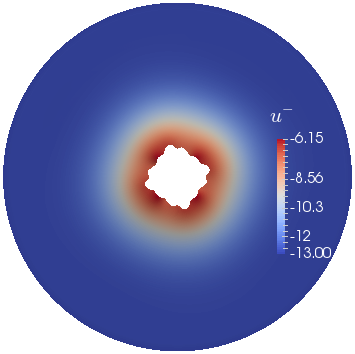
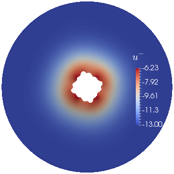
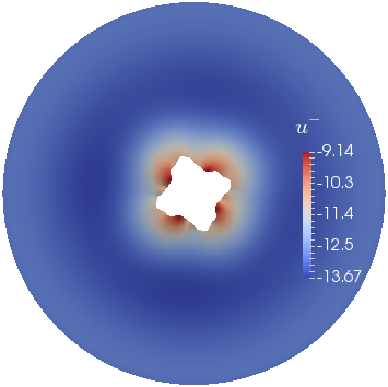
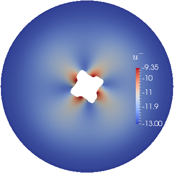
Figure 8: Equilibrium top ($u^{+})$ and bottom ($u^{-}$) membrane surfaces obtained with different initial phase field boundaries at $z=\pm 8,\pm 10,\pm 12,\pm 14\textup{\AA}$, from left to right.

For $z_{ini}=\pm 8\textup{\AA}$ or $\pm 10\textup{\AA}$, the corresponding equilibrated protein-membrane interfaces are identical and located near $z=-6\textup{\AA}$ and $z=8\textup{\AA}$, respectively. The two membrane surfaces have to bend significantly to match these inner boundaries as their exterior boundaries are clamped at $z=\pm 13\textup{\AA}$. This shall generate large bending and compression energies, see also Table 1. When the initial phase boundaries are placed further apart at $|z_{ini}|>11.3\textup{\AA}$, the new bottom protein-membrane interface promotes the curving of the membrane near the protein, shown as the peaking of saddle splay energy in the table, see also the variation of the membrane heights near the protein in Fig. 8, where the four peaks of the displacement signifies the quatermer structure of M2.

$z_{ini}$	$\pm 8$	$\pm 9$	$\pm 10$	$\pm 11$	$\pm 12$	$\pm 13$	$\pm 14$
Splay	-310.7	-305.6	-292.1	-350.2	-365.6	45.72	-183.23
Saddle splay	2.11	1.13	0.96	-6.87	-13.56	27.54	6.99
Surface tension	1.50	1.02	0.65	0.36	0.24	0.60	0.54
Compression	196159	136287	88400	47046	16106	534.2	8382
Tilt-stretch	0.75	0.51	0.32	0.19	0.13	0.20	0.24

Table 1: Energies in $kcal/mol$ corresponding to different modes of bilayer deformation when the initial membrane-protein contact curves are varied.

The significant increase of bilayer compression near the embedded protein from $z_{ini}=\pm 8\textup{\AA}$ to $z_{ini}=\pm 13\textup{\AA}$ is also illustrated in Fig. 9. Maximum energy for saddle splay is observed at $z_{ini}=\pm 13\textup{\AA}$, indicating the largest negative Gaussian curvature is generated, a feature that is well observed in small angle X-ray scattering and molecular dynamics simulations [71, 72]. However, this negative Gaussian curvature is confined to a small neighborhood near the embedded protein.

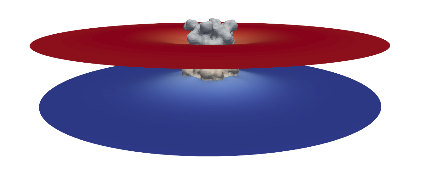
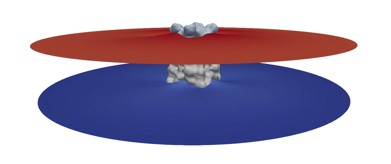
Figure 9: Embedding of M2 channel in the bilayer with $z_{ini}=\pm 8$ (left) and $z_{ini}=\pm 13$ (right).

We attribute this confinement to the homogeneous Dirichlet (aka clamped) boundary condition (26). In experiments the far boundary is not clamped while in molecular dynamics simulations a periodic boundary condition is usually chosen. A more realistic boundary condition on the exterior edge of the annulus would be

$$\Delta u=0,\quad\frac{\partial\Delta u}{\partial n}=0,$$ (40)

i.e., the membrane is stress-free there. However, there does not exist a robust numerical method for biharmonic equations with mixed boundary conditions in arbitrarily complicated 2-D domain. Recently emerged weak Galerkin method might posses the flexibility of approximating forth-order equations with mixed boundary conditions (Dirichlet boundary conditions (29) on the inner edge and stress-free boundary condition on the exterior edge).

5 Conclusion

In this paper we propose a geodesic curvature energy model for characterizing the protein-membrane interfaces. These interfaces represent the essential information of the boundaries in the continuum or hybrid modeling of bilayer membrane morphology induced by embedded proteins. Along with a surface phase field approximation of the geodesic curvature, our efforts present a computationally tractable geometrical characterization of the boundary conditions for the protein-membrane interactions. To further completely couple the surface morphology of two leaflets we first envision an annulus located between two surfaces and then construct conformal mapping between individual surface and the middle annulus through numerical grid generation. We integrate these two new features into a general energetic functional model of protein-membrane interactions. Numerical experiments demonstrate that our methods are efficient and robust in locating the highly complicated protein-membrane interfaces and the corresponding membrane morphology.

Our work can be improved and extended mathematically and computationally in several different directions. A stress-free boundary condition on the exterior edge of membrane shall better reflect the local mechanical constraint and we are currently developing a weak Galerkin finite element method for solving the resulting fourth order equations with mixed boundary conditions. Secondly, the manual scanning on the protein surface for locating a global minimum of total geodesic curvature can be replaced by a surface Allan-Cahn equation with stochastic forcing term (or a stochastic term directly added to the total geodesic curvature energy) that could provide an additional force driving the evolving surface phase boundary from a local minimum to the global minimum. Finally, force and torque balance equations can be introduced to the transmembrane protein to better describe the tilting and orientation of the embedded protein.

References

- [1] G. Guidotti, Membrane proteins, Annual Review of Biochemistry 41 (1) (1972) 731–752, pMID: 4263713. doi:10.1146/annurev.bi.41.070172.003503.
- [2] S. Takamori, M. Holt, K. Stenius, E. A. Lemke, M. Gronborg, D. Riedel, H. Urlaub, S. Schenck, B. Brugger, P. Ringler, S. A. Mueller, B. Rammner, F. Grater, J. S. Hub, B. L. D. Groot, G. Mieskes, Y. Moriyama, J. Klingauf, H. Grubmuller, J. Heuser, F. Wieland, R. Jahn, Molecular anatomy of a trafficking organelle, Cell 127 (4) (2006) 831 – 846. doi:10.1016/j.cell.2006.10.030.
- [3] O. S. Andersen, R. E. Koeppe, Bilayer thickness and membrane protein function: An energetic perspective, Annu. Rev. Biophys. Biomol. Struct. 36 (1) (2007) 107–130. doi:10.1146/annurev.biophys.36.040306.132643.
- [4] S. Sukharev, F. Sachs, Molecular force transduction by ion channels – diversity and unifying principles, J. Cell Sci. 125 (13) (2012) 3075–3083. doi:10.1242/jcs.092353.
- [5] K. I. Lee, R. W. Pastor, O. S. Andersen, W. Im, Assessing smectic liquid-crystal continuum models for elastic bilayer deformations, Chem. Phys. Lipids 169 (2013) 19 – 26. doi:10.1016/j.chemphyslip.2013.01.005.
- [6] S. Choe, K. A. Hecht, M. Grabe, A continuum method for determining membrane protein insertion energies and the problem of charged residues, J. Gen. Physiol. 131 (2008) 563–6573. doi:10.1085/jgp.200809959.
- [7] Y. C. Zhou, B. Lu, A. A. Gorfe, Continuum electromechanical modeling of protein-membrane interactions, Phys. Rev. E 82 (4) (2010) 041923. doi:10.1103/PhysRevE.82.041923.
- [8] X. Chen, Q. Cui, Computational molecular biomechanics: A hierarchical multiscale framework with applications to gating of mechanosensitive channels of large conductance, in: T. Dumitrica (Ed.), Trends in Computational Nanomechanics, Vol. 9 of Challenges and Advances in Computational Chemistry and Physics, Springer Netherlands, 2010, pp. 535–556.
- [9] J. K. Sigurdsson, F. L. Brown, P. J. Atzberger, Hybrid continuum-particle method for fluctuating lipid bilayer membranes with diffusing protein inclusions, J. Comput. Phys. 252 (0) (2013) 65 – 85. doi:10.1016/j.jcp.2013.06.016.
- [10] D. Argudo, N. P. Bethel, F. V. Marcoline, C. W. Wolgemuth, M. Grabe, New continuum approaches for determining protein-induced membrane deformations, Biophys. J.doi:10.1016/j.bpj.2017.03.040.
- [11] P. B. Canham, The minimum energy of bending as a possible explanation of the biconcave shape of the human red blood cell, J. Math. Biol. 26 (1970) 61–81.
- [12] W. Helfrich, Elastic properties of lipid bilayers: theory and possible experiments, Z. Naturforsch 28c (1973) 693–703.
- [13] E. Evans, Bending resistance and chemically induced moments in membrane bilayers, Biophys. J. 14 (1974) 923–931.
- [14] T. Kim, K. I. Lee, P. Morris, R. W. Pastor, O. S. Andersen, W. Im, Influence of hydrophobic mismatch on structures and dynamics of gramicidin A and lipid bilayers, Biophys. J. 102 (7) (2012) 1551–1560. doi:10.1016/j.bpj.2012.03.014.
- [15] Y. Tang, G. Cao, X. Chen, J. Yoo, A. Yethiraj, Q. Cui, A finite element framework for studying the mechanical response of macromolecules: application to the gating of machanosensitive channel MscL, Biophys. J. 91 (2006) 1248–1263. doi:10.1529/biophysj.106.085985.
- [16] M. Feig, G. Nawrocki, I. Yu, P. hung Wang, Y. Sugita, Challenges and opportunities in connecting simulations with experiments via molecular dynamics of cellular environments, J. Phys. Conf. Ser. 1036 (2018) 012910. doi:10.1088/1742-6596/1036/1/012010.
- [17] N. Bavi, C. D. Cortes, D. Marienand Cox, P. R. Rohde, W. Liu, J. W. Deitmer, O. Bavi, P. Strop, A. P. Hill, D. Rees, B. Corry, E. Perozo, B. Martinac, The role of MscL amphipathic n terminus indicates a blueprint for bilayer-mediated gating of mechanosensitive channels, Nature Commun. 7 (2016) 11984. doi:10.1038/ncomms11984.
- [18] J. B. Fournier, Nontopological saddle-splay and curvature instabilities from anisotropic membrane inclusions, Phys. Rev. Lett. 76 (1996) 4436–4439. doi:10.1103/PhysRevLett.76.4436.
- [19] H. Noguchi, J.-B. Fournier, Membrane structure formation induced by two types of banana-shaped proteins, Soft Matter 13 (2017) 4099–4111. doi:10.1039/C7SM00305F.
- [20] Y. C. Zhou, On curvature driven rotational diffusion of proteins on membrane surfaces, SIAM J. Appl. Math. In Press (2019).
- [21] K. M. Callenberg, N. R. Latorraca, M. Grabe, Membrane bending is critical for the stability of voltage sensor segments in the membrane, J. Gen. Physiol. 140 (1) (2012) 55–68. doi:10.1085/jgp.201110766.
- [22] M. Adkins, Y. C. Zhou, Geodesic curvature driven surface microdomain formation, J. Comput. Phys. 345 (2017) 260–274. doi:https://doi.org/10.1016/j.jcp.2017.05.029.
- [23] R. A. Pierotti, A scaled particle theory of aqueous and nonaqueous solutions, Chem. Rev. 76 (1976) 717–726. doi:10.1021/cr60304a002.
- [24] J. A. Wagoner, N. A. Baker, Assessing implicit models for nonpolar mean solvation forces: The importance of dispersion and volume terms, P. Natl. Acad. Sci. USA 103 (22) (2006) 8331–8336. doi:10.1073/pnas.0600118103.
- [25] M. A. Grayson, Shortening embedded curves, Ann. Math. 129 (1989) 71–111. doi:10.2307/1971486.
- [26] M. E. Gage, Curve shortening on surfaces, Annales scientifiques de l’École Normale Supérieure Ser. 4, 23 (2) (1990) 229–256. doi:10.24033/asens.1603.
- [27] S. Osher, J. A. Sethian, Fronts propagating with curvature-dependent speed: Algorithms based on Hamilton-Jacobi formulations, J. Comput. Phys. 79 (1) (1988) 12 – 49. doi:10.1016/0021-9991(88)90002-2.
- [28] J. A. Sethian, Level Set Methods and Fast Marching Methods, 2nd Edition, Cambridge University Press, 1999.
- [29] C. Wu, X.-C. Tai, A level set formulation of geodesic curvature flow on simplicial surfaces, IEEE Trans. Vis. Comput. Graph. 16 (2010) 647–662. doi:10.1109/TVCG.2009.103.
- [30] Z. Liu, H. Zhang, C. Wu, On geodesic curvature flow with level set formulation over triangulated surfaces, J. Sci. Comput. 70 (2) (2017) 631–661. doi:10.1007/s10915-016-0260-3.
- [31] J. Y. Wang, S. Betelu, B. M. Law, Line tension approaching a first-order wetting transition: Experimental results from contact angle measurements, Phys. Rev. E 63 (2001) 031601. doi:10.1103/PhysRevE.63.031601.
- [32] U. O. M. Vázquez, W. Shinoda, P. B. Moore, C.-C. Chiu, S. O. Nielsen, Calculating the surface tension between a flat solid and a liquid: a theoretical and computer simulation study of three topologically different methods, J. Math. Chem. 45 (1) (2009) 161–174. doi:10.1007/s10910-008-9374-7.
- [33] D. Argudo, N. Bethel, F. Marcoline, M. Grabe, Continuum descriptions of membranes and their interaction with proteins: Towards chemically accurate models, BBA-Biomembranes 1858 (2016) 1619–1634. doi:10.1016/j.bbamem.2016.02.003.
- [34] M. Hamm, M. M. Kozlov, Elastic energy of tilt and bending of fluid membranes, Euro. Phys. J. E 3 (4) (2000) 323–335. doi:epje/v3/p323(e0025).
- [35] M. S. Jablin, K. Akabori, J. F. Nagle, Experimental support for tilt-dependent theory of biomembrane mechanics, Phys. Rev. Lett. 113 (2014) 248102. doi:10.1103/PhysRevLett.113.248102.
- [36] R. J. Ryham, T. S. Klotz, J. Yao, F. S. Cohen, Calculating transition energy barriers and characterizing activation states for steps of fusion, Biophys. J. 110 (5) (2016) 1110 – 1124. doi:10.1016/j.bpj.2016.01.013.
- [37] J. P. Bardhan, Nonlocal continuum electrostatic theory predicts surprisingly small energetic penalties for charge burial in proteins, J. Chem. Phys. 135 (2011) 104113. doi:10.1063/1.3632995.
- [38] A. Hildebrandt, R. Blossey, S. Rjasanow, O. Kohlbacher, H.-P. Lenhof, Novel formulation of nonlocal electrostatics, Phys. Rev. Lett. 93 (2004) 108104. doi:10.1103/PhysRevLett.93.108104.
- [39] D. Xie, Y. Jiang, L. R. Scott, Efficient algorithms for a nonlocal dielectric model for protein in ionic solvent, SIAM J. Sci. Comput. 35 (2013) 1267–1284. doi:10.1137/120899078.
- [40] B. Li, Continuum electrostatics for ionic solutions with non-uniform ionic sizes, Nonlinearity 22 (2009) 811. doi:10.1088/0951-7715/22/4/007.
- [41] B. Lu, Y. C. Zhou, Poisson-Nernst-Planck equations for simulating biomolecular diffusion-reaction processes II: Size effects on ionic distributions and diffusion-reaction rates, Biophys. J. 100 (2011) 2475–2485. doi:10.1016/j.bpj.2011.03.059.
- [42] M. Mikucki, Y. C. Zhou, Electrostatic forces on charged surfaces of bilayer lipid membranes, SIAM J. Appl. Math. 74 (2014) 1–21. doi:10.1137/130904600.
- [43] D. Sitkoff, N. Bental, B. Honig, Calculation of alkane to water solvation free energies using continuum solvent models, J. Phys. Chem. 100 (7) (1996) 2744–2752. doi:10.1021/jp952986i.
- [44] Z. Chen, S. Zhao, J. Chun, D. G. Thomas, N. A. Baker, P. W. Bates, G. W. Wei, Variational approach for nonpolar solvation analysis, J. Chem. Phys. 137 (8). doi:10.1063/1.4745084.
- [45] R. S. Cantor, The lateral pressure profile in membranes: A physical mechanism of general anesthesia, Biochem. 36 (9) (1997) 2339–2344. doi:10.1021/bi9627323.
- [46] R. S. Cantor, Lipid composition and the lateral pressure profile in bilayers., Biophys. J. 76 (1999) 2625–2639. doi:10.1016/S0006-3495(99)77415-1.
- [47] D. Marsh, Lipid Bilayer Lateral Pressure Profile, Springer Berlin Heidelberg, Berlin, Heidelberg, 2013, pp. 1253–1256. doi:10.1007/978-3-642-16712-6_544.
- [48] D. Marsh, Lateral pressure profile, spontaneous curvature frustration, and the incorporation and conformation of proteins in membranes, Biophys. J. 93 (2007) 3884–3899. doi:10.1529/biophysj.107.107938.
- [49] A. A. Drozdova, S. I. Mukhin, Lateral pressure profile in bent lipid membranes and mechanosensitive channels gating, bioRxivdoi:10.1101/062463.
- [50] B. Li, Minimization of electrostatic free energy and the Poisson-Boltzmann equation for molecular solvation with implicit solvent, SIAM J. Math. Anal. 40 (2009) 2536–2566. doi:10.1137/080712350.
- [51] G.-W. Wei, Differential geometry based multiscale models, Bull. Math. Biol. 72 (6) (2010) 1562–1622. doi:10.1007/s11538-010-9511-x.
- [52] Q. Du, L. Ju, L. Tian, Finite element approximation of the Cahn-Hilliard equation on surfaces, Comput. Methods Appl. Mech. Eng. 200 (29?32) (2011) 2458 – 2470. doi:10.1016/j.cma.2011.04.018.
- [53] V. Caselles, R. Kimmel, G. Sapiro, Geodesic active contours, Int. J. of Comput. Vis. 22 (1) (1997) 61–79. doi:10.1023/A:1007979827043.
- [54] A. Spira, R. Kimmel, Geometric curve flows on parametric manifolds, J. Comput. Phys. 223 (1) (2007) 235–249. doi:https://doi.org/10.1016/j.jcp.2006.09.008.
- [55] K. Bohinc, V. Kralj-Iglic, S. May, Interaction between two cylindrical inclusions in a symmetric lipid bilayer, J. Chem. Phys. 119 (14) (2003) 7435–7444. doi:10.1063/1.1607305.
- [56] S. May, Membrane perturbations induced by integral proteins: Role of conformational restrictions of the lipid chains, Langmuir 18 (16) (2002) 6356–6364. doi:10.1021/la025747c.
- [57] Y. C. Zhou, M. Feig, G. W. Wei, Highly accurate biomolecular electrostatics in continuum dielectric environments, J. Comput. Chem. 29 (2008) 87–97. doi:10.1002/jcc.20769.
- [58] B. Lu, Y. C. Zhou, M. Holst, J. A. McCammon, Recent progress in numerical solution of the Poisson-Boltzmann equation for biophysical applications, Commun. Comput. Phys. 3 (2008) 973–1009.
- [59] A. Der, L. Kelemen, L. Fabian, S. G. Taneva, E. Fodor, T. Pali, A. Cupane, M. G. Cacace, J. J. Ramsden, Interfacial water structure controls protein conformation, J. Phys. Chem. B 111 (19) (2007) 5344–5350. doi:10.1021/jp066206p.
- [60] W. Geng, R. Krasny, A treecode-accelerated boundary integral Poisson-Boltzmann solver for electrostatics of solvated biomolecules, J. Comput. Phys. 247 (2013) 62–78. doi:10.1016/j.jcp.2013.03.056.
- [61] J. Chen, W. Geng, On preconditioning the treecode-accelerated boundary integral (tabi) Poisson-Boltzmann solver, J. Comput. Phys. 373 (2018) 750–762. doi:10.1016/j.jcp.2018.07.011.
- [62] S. C. Brenner, S. Gu, T. Gudi, L. yeng Sung, A quadratic c0 interior penalty method for linear fourth order boundary value problems with boundary conditions of the Cahn-Hilliard type, SIAM J. Numer. Anal. 50 (4) (2012) 2088–2110. doi:10.1137/110847469.
- [63] E. H. Georgoulis, P. Houston, Discontinuous Galerkin methods for the biharmonic problem, IMA J. Numer. Anal. 29 (3) (2008) 573–594. doi:10.1093/imanum/drn015.
- [64] P. Knupp, S. Steinberg, Fundamentals of grid generation, CRC Press, 1993.
- [65] C. M. Elliott, A. M. Stuart, The global dynamics of discrete semilinear parabolic equations, SIAM J. Numer. Anal. 30 (6) (1993) 1622–1663. doi:10.1137/0730084.
- [66] J. Shen, C. Wang, X. Wang, S. M. Wise, Second-order convex splitting schemes for gradient flows with Ehrlich-Schwoebel type energy: Application to thin film epitaxy, SIAM J. Numer. Anal. 50 (2012) 105–125. doi:10.1137/110822839.
- [67] Z. Hu, S. Wise, C. Wang, J. Lowengrub, Stable and efficient finite-difference nonlinear-multigrid schemes for the phase field crystal equation, J. Comput. Phys. 228 (15) (2009) 5323 – 5339. doi:10.1016/j.jcp.2009.04.020.
- [68] X. Wang, L. Ju, Q. Du, Efficient and stable exponential time differencing runge-kutta methods for phase field elastic bending energy models, J. Comput. Phys. 316 (2016) 21 – 39. doi:10.1016/j.jcp.2016.04.004.
- [69] X. Yang, L. Ju, Efficient linear schemes with unconditional energy stability for the phase field elastic bending energy model, Comput. Methods Appl. Mech. Eng. 315 (2017) 691 – 712. doi:10.1016/j.cma.2016.10.041.
- [70] R. Chen, G. Ji, X. Yang, H. Zhang, Decoupled energy stable schemes for phase-field vesicle membrane model, J. Comput. Phys. 302 (2015) 509 – 523. doi:10.1016/j.jcp.2015.09.025.
- [71] N. W. Schmidt, A. Mishra, J. Wang, W. F. DeGrado, G. C. L. Wong, Influenza virus A M2 protein generates negative Gaussian membrane curvature necessary for budding and scission, J. Am. Chem. Soc. 135 (37) (2013) 13710. doi:10.1021/ja400146z.
- [72] J. Paulino, X. Pang, I. Hung, H.-X. Zhou, T. A. Cross, Influenza A M2 channel clustering at high protein/lipid ratios: Viral budding implications, Biophys. J. 116 (6) (2019) 1075 – 1084. doi:10.1016/j.bpj.2019.01.042.
- [73] S. A. Safran, Mark O. Robbins, S. Garoff, Tilt and splay of surfactants on surfaces, Phys. Lett. A 33 (3) (1986) 2186 – 2189. doi:10.1103/physreva.33.2186.