MTAdam: Automatic Balancing of
Multiple Training Loss Terms

Abstract

When training neural models, it is common to combine multiple loss terms. The balancing of these terms requires considerable human effort and is computationally demanding. Moreover, the optimal trade-off between the loss term can change as training progresses, especially for adversarial terms. In this work, we generalize the Adam optimization algorithm to handle multiple loss terms. The guiding principle is that for every layer, the gradient magnitude of the terms should be balanced. To this end, the Multi-Term Adam (MTAdam) computes the derivative of each loss term separately, infers the first and second moments per parameter and loss term, and calculates a first moment for the magnitude per layer of the gradients arising from each loss. This magnitude is used to continuously balance the gradients across all layers, in a manner that both varies from one layer to the next and dynamically changes over time. Our results show that training with the new method leads to fast recovery from suboptimal initial loss weighting and to training outcomes that match conventional training with the prescribed hyperparameters of each method. MTAdam code can be found here.

1 Introduction

In both supervised and unsupervised image generation tasks, one tries to balance a set of criteria, some overlapping and some presenting natural tradeoffs. For example, in image analogy tasks, multiple conditioned generation criteria, some based on comparing the input to the output using an MSE term and some on perceptual losses, may be combined with one or more adversarial losses. If the mapping is two-sided, one also employs a circularity loss. If the image is of a composite nature, mask-based losses are added, and so on.

It has been demonstrated repeatedly that adding losses can be beneficial. In many cases, formulating the desiderata as loss terms is well paved. However, as more loss terms are added, the space of possible balancing weights increases exponentially, and more resources need to be allocated to identify good configurations that would justify the added terms. Another common challenge is that at different stages of the training process, the optimal balance may change [18]. This is especially true for adversarial losses, which often become unstable. It is, therefore, necessary to have the balancing terms update dynamically during training.

In this work, we introduce Multi-Term Adam (MTAdam), an optimization algorithm for multi-term loss functions. MTAdam extends Adam [13] and allows an effective training of an unweighted multi-term loss objective. Thus, MTAdam can streamline the computationally demanding task of hyperparameter search, required for effectively weighting multi-term loss objectives.

At every training iteration, a dynamic weight is assigned to each of the loss terms based on the magnitude of the gradient that each term entails. The weights are assigned in a way that balances between these gradients and equates their magnitude.

This, however, would be an ineffective balancing method, without three crucial components: (i) the balancing needs to occur independently for each layer of the neural network, since the relative contributions of the losses vary, depending on the layer, (ii) the balancing needs to be anchored by a dominant loss term in order to allow a natural progression of the effective learning rate, i.e., one cannot normalize such that the magnitude becomes a constant, and (iii) the update step needs to take into account the maximal variance among all losses, to support sufficient explorations in places of the parameter space, in which one of the losses becomes more sensitive.

The main focus of our experiments is in the field of conditional adversarial image generation. This domain is known to require multiple loss terms. Moreover, the quality of the generated images is evaluated using acceptable success metrics that are not directly optimized by any of the loss terms, such as FID [8]. Our results show that MTAdam is able to recover from unbalanced starting points, in which the weight parameters are set inappropriately, while Adam and other baseline methods cannot.

2 Related Work

SGD with momentum (Nesterov) [20] is an optimization algorithm that extends SGD, suggesting to update the network’s parameters by a moving average of the gradients, rather than the gradients at each step. Root Mean Square Propagation (RMSProp) [23] extends SGD by dividing the learning rate during the backward step, by the moving average of the second moment of the gradients of each parameter. Adam [13] combines both principles and employs the first and second moments of the gradients of each learned parameter and applies them during the backward step. Adam has become a dominant optimizer, that is applied across many applications, and, in particular, it is the de-facto standard in the field of adversarial training. It is known for improving convergence to work well with the default values of its own hyperparameters ($\beta_{1}$ and $\beta_{2}$).

Multiple methods have been suggested for selecting hyperparameters [22, 26, 1, 5]. Hyperband [15] performs hyperparameter search as an infinite-armed bandit problem utilizing a predefined amount of resources while searching for the best configuration of hyperparameters that maximizes the given success criterion. It can provide an order-of-magnitude speedup compared to Bayesian optimization [1, 21, 9]. We utilize Hyperband as a baseline that can directly optimize the FID score.

Image generation techniques utilize multiple loss terms, including pixel-wise norms, perceptual losses [11], and one or more adversarial loss terms [6]. The need for a careful configuration of the weight parameters hinders research in this field and increases its costs.

In our experiments, we employ three different image generation methods, which vary in the type of supervision employed or the task being solved: (i) pix2pix [10] generates an image in domain $B$ based on an input image in domain $A$, after observing matching pairs during training. (ii) CyclgeGAN [29] performs the same task while training in an unsupervised manner on unmatched images from the two domains. (iii) SRGAN [14] generates high-resolution images from low-resolution ones and is trained in a supervised way.

Multi-task learning shares some similarities with multi-term learning. In multi-task learning, one learns a few tasks concurrently, each associated with one or more loss terms. The most common approaches utilize hard parameter sharing [2, 12, 7, 16, 19], in which a single model, with multiple task-specific heads, is trained. This approach is extremely effective when the tasks are highly related, as in MaskRCNN [7]. In the soft parameter sharing approach, each task has its own model, and a regularization term encourages the parameters of the different models to be similar [27, 4]. While MTAdam can be applied to multi-task learning (of both types) without substantial modifications, we leave the empirical validation of this ability for future investigations.

3 Method

The Adam algorithm optimized one stochastic objective function $f_{t}(\theta)$ over the set of parameters $\theta$, where $t$ is an index of the current mini-batch of samples. In contrast, MTAdam optimizes a set of such terms $f_{t}^{1}(\theta),\dots,f_{t}^{I}(\theta)$. While Adam’s task is to minimize the expected value $E_{t}[f_{t}(\theta)]$ w.r.t. the parameters $\theta$, MTAdam minimizes a weighted average of the $I$ terms. The weights of these mixtures are all positive, but otherwise unknown. The guiding principle for the determination of the weights at each iteration $t$ is that the moving average of the magnitude of the gradient of each term is equal across terms. This magnitude is evaluated and balanced at every layer of the neural network.

In Adam, two moments are continuously updated, using a moving average scheme: $m_{t}$ is the first moment of the gradient $\nabla_{\theta}f_{t}$ and $v_{t}$ is the second moment. Both are vectors of the same size of $\theta$. The moving averages are computed using the mixing coefficients $\beta_{1}$ and $\beta_{2}$ for the two moments.

MTAdam records such moments for each term $i=1...I$ separately. In addition, it uses a mixing coefficient $\beta_{3}$ in order to maintain the moving average of the gradient magnitude per each layer $\ell$, which is denoted by $n_{l,t}^{i}$.

Adam borrows from the SGD with momentum method (Nesterov) and updates the vector of parameters based on the weighted first moment of the gradient. In MTAdam, the first moment is computed based on a weighted gradient, in which the parameters of each layer $\ell$ for every term $i$ are weighted such that their magnitude is normalized by the factor $n_{\ell,t}^{i}$. This way, across all layers, and at every time point, the $I$ terms contribute equally to the gradient step.

The Adam optimization algorithm is depicted in the left side of Alg. 1 and MTAdam on the right. In line 1, MTAdam algorithm initializes $I$ pairs of first and second moment vectors. This is similar to Adam, except for initializing a pair of moments for each loss term. In line 2, and different from Adam, MTAdam initializes $I$ first moments for the magnitude of the gradients, per layer. In line 3, both MTAdam and Adam iterate over the stochastic mini-batches, performing $T$ training steps.

In line 4, MTAdam iterates over the loss terms. For each loss term, MTAdam calculates its gradients over each one of the network layers (line 5), in an analogous manner to the way Adam computes the (single) gradients vector $\nabla_{\theta}f_{t}(\theta_{t}-1)$. In lines 6-8, MTAdam iterates over the layers, updates the moving average of the magnitude for each layer and loss term, and normalizes the gradients of the current layer and loss term, by multiplying with $\frac{n_{\ell,t}^{1}}{n_{\ell,t}^{i}}$. This multiplication normalizes the magnitude of the current gradients of layer $\ell$ and loss term $i$ using the moving average $n_{\ell}^{i}$. This normalization leads to all gradient magnitudes to be similar to that of the first loss term.

In line 5, we calculate the gradients of each specific loss term $i$ w.r.t $\theta$, across all layers. For a layer index $\ell$, the gradient is denoted by $g_{\ell}^{i}$. We denoted by $g^{i}$ the concatenation of all per-layer gradients.

Lines 6-8 of MTAdam do not have an Adam analog. The operation performed normalizes the magnitude of the gradients of all loss terms, to match the magnitude of the first loss term. This assigns a unique role to the first term, as the primary loss to which all other losses are compared. By linking the magnitude to that of a concrete loss, and not to a static value (e.g., normalizing to have a unit norm), we maintain the relationship between the training progression and the learning rate.

The normalization iterates over the loss terms, and for each gradient, the first moment of the magnitude of the gradient is updated. The gradient magnitude is then normalized by that of the first loss term.

Then, in lines 9-12, MTAdam updates the first and second moments for each parameter and each loss term and computes their bias correction. This is similar to Adam, except that the moments are calculated separately for each loss term. In lines 13-15, MTAdam iterates over the loss terms and calculates the steps from each term. The steps are summed over $\theta_{t-1}$, and the result is assigned $\theta_{t}$.

In Adam, the update size is normalized by the second moment. In MTAdam, we divided by the maximal second moment among all loss terms. This division allows MTAdam to make smaller gradient steps, when a lower certainty is introduced by at least one of the loss terms. The motivation for this is that even if one of the losses is in a high-sensitivity region, where small updates create rapid changes to this term, then the step, regardless of the term which led to it, should be small. The importance of this maximization is demonstrated in the ablation study in Sec. 4.3.

Input: $\alpha$: step size, $\{\beta_{1},\beta_{2}\}$: decay rates to

calculate the first and second moments, $\theta_{0}$:

initial weights, $f_{t}(\theta)$: stochastic objective.

Output: $\theta_{t}$: resulting parameters

1 $m_{0},v_{0}\leftarrow 0,0$

2

3 while $t=\{1,\cdots,T\}$ do

4      

5       $g\leftarrow\nabla_{\theta}f_{t}(\theta_{t-1})$

6      

7      

8      

9       $m_{t}\leftarrow\beta_{1}\cdot m_{t-1}+\left(1-\beta_{1}\right)\cdot g$

10      

11      $v_{t}\leftarrow\beta_{2}\cdot v_{t-1}+\left(1-\beta_{2}\right)\cdot{g^{2}}$

12      

13      $\widehat{m_{t}}\leftarrow m_{t}/\left(1-\beta_{1}^{t}\right)$

14      

15      $\widehat{v_{t}}\leftarrow v_{t}/\left(1-\beta_{2}^{t}\right)$

16      

17       $\theta_{t}\leftarrow\theta_{t-1}-\alpha\cdot\widehat{m_{t}}/(\sqrt{\widehat{v_{t}}}+\epsilon)$

18      

19      

20return $\theta_{T}$

1

Input: In addition to Adam’s parameters: $\beta_{3}$: decay rate for the gradient’s norm first moment, $f^{1}_{t}(\theta)$…$f^{I}_{t}(\theta)$: stochastic loss term functions.

Output: $\theta_{t}$: resulting parameters

2 for $i=\{1,\cdots,I\}$ do  $m^{i}_{0},v^{i}_{0}\leftarrow 0,0$

3 for $l$ in $1...L$ do  $n_{\ell,0}^{i}\leftarrow 1$

4 while $t=\{1,\cdots,T\}$ do

5       for $i=\{1,\cdots,I\}$ do

6             $g^{i}$ := $(g^{i}_{1},...g^{i}_{L})$ $\leftarrow\nabla_{\theta}f^{i}_{t}(\theta_{t-1})$

7            for $\ell$ in $1...L$ do

8                  

9                  $n_{\ell,t}^{i}\leftarrow\beta_{3}\cdot n_{\ell,t-1}^{i}+\left(1-\beta_{3}\right)\cdot{\lVert g^{i}_{\ell}\rVert}_{2}$

10                  $g^{i}_{\ell}\leftarrow n_{\ell,t}^{1}\cdot g^{i}_{\ell}/(n_{\ell,t}^{i})$

11            

12            $m^{i}_{t}\leftarrow\beta_{1}\cdot m^{i}_{t-1}+\left(1-\beta_{1}\right)\cdot g^{i}$

13            

14            $v^{i}_{t}\leftarrow\beta_{2}\cdot v^{i}_{t-1}+\left(1-\beta_{2}\right)\cdot{(g^{i})}^{2}$

15            

16            $\widehat{m^{i}_{t}}\leftarrow m^{i}_{t}/\left(1-\beta_{1}^{t}\right)$

17            

18            $\widehat{v^{i}_{t}}\leftarrow v^{i}_{t}/\left(1-\beta_{2}^{t}\right)$

19            

20      

21      for $i=\{1,\cdots,I\}$ do

22             $\theta_{t-1}\leftarrow\theta_{t-1}-\alpha\cdot\widehat{m^{i}_{t}}/(\sqrt{\max(\widehat{v^{1}_{t}}...\widehat{v^{I}_{t}}})+\epsilon)$

23      $\theta_{t}\leftarrow\theta_{t-1}$

return $\theta_{T}$

Algorithm 1 Adam (left) and Multi-term Adam (right). All operations are element-wise.

Memory and Run Time Analysis  Adam utilizes a pair of 1st and 2nd moments for each learned parameter. Given a network with $\lVert\theta\rVert$ learned parameters, it has a memory complexity of $O({|\theta|})$. MTAdam utilizes $I$ different pairs of 1st and 2nd moments for each parameter. In addition, MTAdam employs $I$ first moments magnitude for each layer. These two extensions bring the memory complexity to $O(I{|\theta|}+IL)\sim O(I{|\theta|})$. In MTAdam, the run time complexity also depends on the number of loss terms $O(I\theta)$. The dependence on the number of layers $L$ in Alg. 1 can be absorbed in $\Theta$.

4 Experiments

We compare the results of MTAdam with five baselines: (1-3) Adam, RMSProp, and SGD with momentum, applied with unbalanced weightings. (4) Hyperband [15] applied to perform a hyper-parameter search for the lambdas between the loss terms, utilizing the FID metric. (5) Adam optimizer applied with a balanced weighting.

We note that baseline (4) benefits from running training multiple times and that baseline (5) employs the weights proposed for each method after a development process that is likely to have included a hyper-parameter search, in which multiple runs were evaluated by the developers of each method. For each optimization method, we employ the default parameters in pytorch. For the Adam experiments, we set the hyperparameters $\beta_{1}$ and $\beta_{2}$ to 0.9 and 0.999, respectively. For MTAdam, $\beta_{1}$ and $\beta_{2}$ are configured with the same values as Adam and $\beta_{3}=0.9$.

4.1 MNIST classification

In order to turn MNIST to an unbalanced multi-term experiment, we compute the loss for each of the digits separately, creating ten loss terms, each weighted by a random weight from the uniform distribution between 1 and 1000. The test set is unweighted, which causes classes that are associated with lower weights to suffer from underfitting.

The official of the pytorch MNIST example is used: two convolutional layers followed by two fully connoted layers. The experiment is repeated 100 times, and for the sake of saving computations, hyperband is not tested. The results in Tab. 1, show a clear advantage for MTAdam over the other unbalanced alternatives.

Table 1: MNIST results. Shown is mean accuracy in percents and SD for 100 runs.

Unbalanced				Balanced
SGD-Momentum	RMSProp	Adam	MTAdam	Adam
85.4 $\pm$ 1.23	87.2 $\pm$ 0.97	88.8 $\pm$ 0.84	97.9 $\pm$ 0.07	98.3 $\pm$ 0.05

4.2 Image synthesis

We demonstrate the ability of MTAdam to effectively converge when applied with unbalanced multi-term loss objectives. To this end, we compare the performance of MTAdam with other optimizers, evaluated on three methods, pix2pix [10], CycleGan [29] and SRGAN [14].

We used the learning rate as found in the implementation of each method [10, 29, 14]. Performance is evaluated using various metrics: L1, L2, PSNR, NMSE (normalized MSE), FID [8], and SSIM [25]. In each case, following the metrics used in the original work, with the addition of FID.

Figure 1: (left) L1 and (right) FID per epoch on the validation set of Facade for three pix2pix variants. Balanced-Adam and Unbalanced-Adam employ Adam, with a balanced and unbalanced weighting, respectively. Unbalanced-MTAdam utilizes MTAdam.

Figure 2: Samples from the Facade test set. Balanced-Adam employs pix2pix with the prescribed weights [10]. Unbalanced-Adam runs with equal initial weights, which leads to visual artifacts. Unbalanced-MTAdam (our method) starts with equal weights, but produces images of the same quality as Balanced-Adam.

Pix2pix Experiments  The objective function of the pix2pix generator has dual-terms:

$$\pazocal{L}_{pix2pix}=\lambda_{1}\pazocal{L}_{1}+\lambda_{2}\pazocal{L}_{GAN}$$ (1)

Where $\pazocal{L}_{GAN}$ is the GAN loss of the generator, $\pazocal{L}_{1}$ is the pixel loss, and $\lambda_{1}$ and $\lambda_{2}$ are set to 100 and 1, respectively. In our study, we unbalance pix2pix models by setting $\lambda_{2}$ to 100 (which implies a 1:1 ratio between the two loss terms).

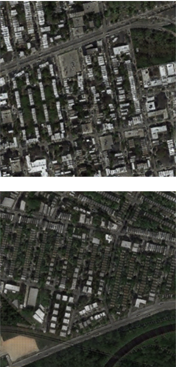
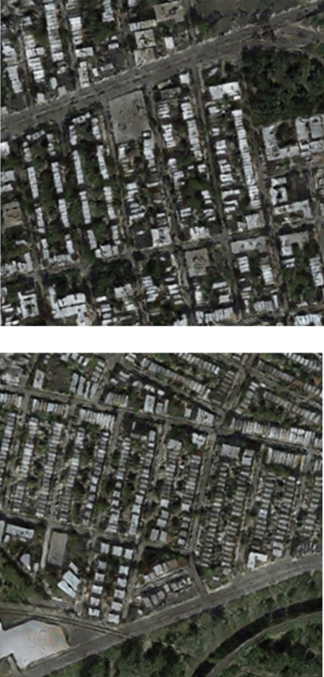
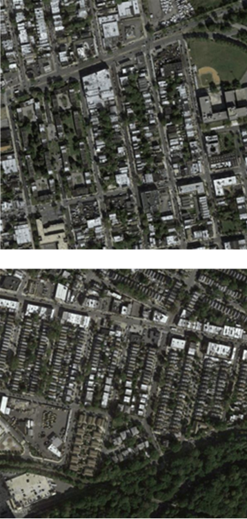
Two datasets are used: matching facade images and their semantic labels [24] and aerial photographs and matching maps [10]. Performance is reported on a holdout test set of each benchmark.

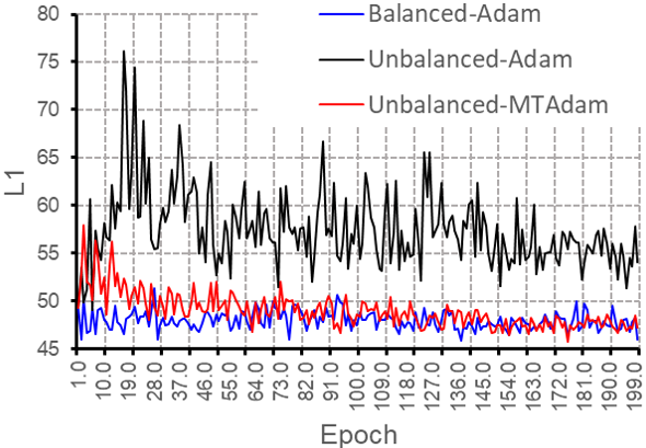
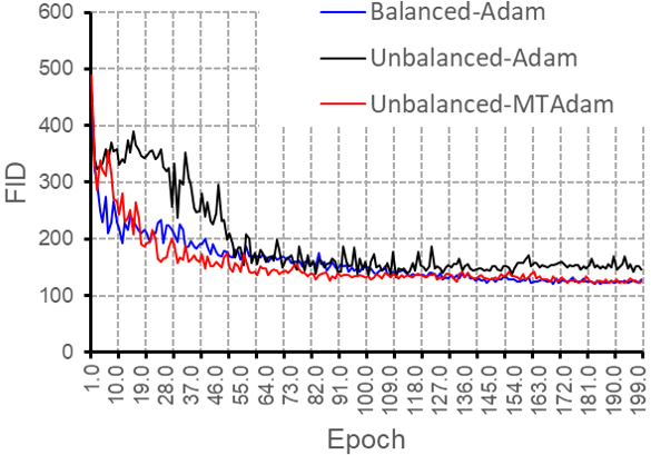
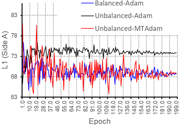
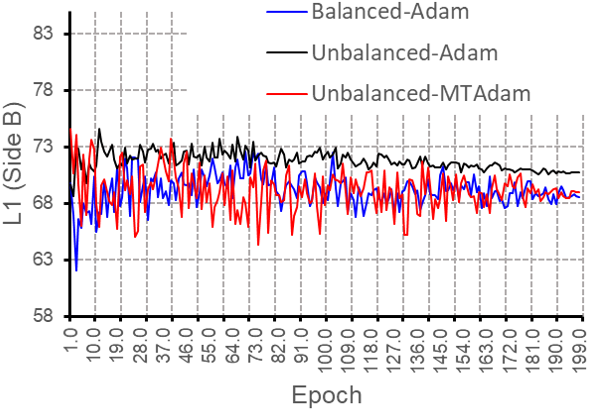
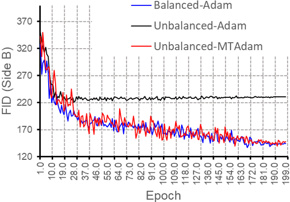
Fig. 1, depicts the test-performance of multiple models per each training epoch. The experiment’s name contains ‘unbalanced’ for the case of equal loss terms, and ‘balanced’ when using the prescribed $\lambda$ values. As can be seen, unbalanced-MTAdam yields a similar convergence as the balanced-Adam. Specifically, the MTAdam experiment converges substantially better than the unbalanced Adam experiment, leading to improved L1 and FID scores.

In Tab. 2 MTAdam is compared with all baselines, applied for training pix2pix models. The top four models, in each section, utilize an identical unbalanced setting, each applied with a different optimizer. The Hyperband experiment utilizes the FID metric to perform a hyperparameter search on $\lambda_{2}$. The Hyperband experiments incorporate 40 trials (i.e. 40 training processes, which gives it a great advantage), each trial randomly sampled a different lambda from the range $[10^{-4},10^{4}]$. We report Hyperband performance by utilizing the trial that is associated with the chosen lambda. In the aerial photograph experiment, the Hyperband failed to choose a $\lambda_{2}$ value that is close to the original value of 1. In the facade experiment, Hyperband sampled at least one lambda value between 0.5 to 10, yet the retrieved best model utilizes a higher lambda value of 162.89, since this value showed a preferable FID value on the validation set. In the maps dataset, a value of 59.61 was selected.

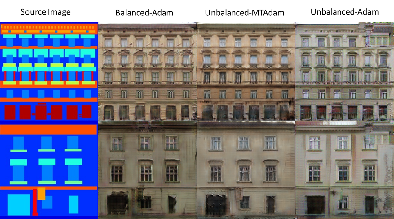
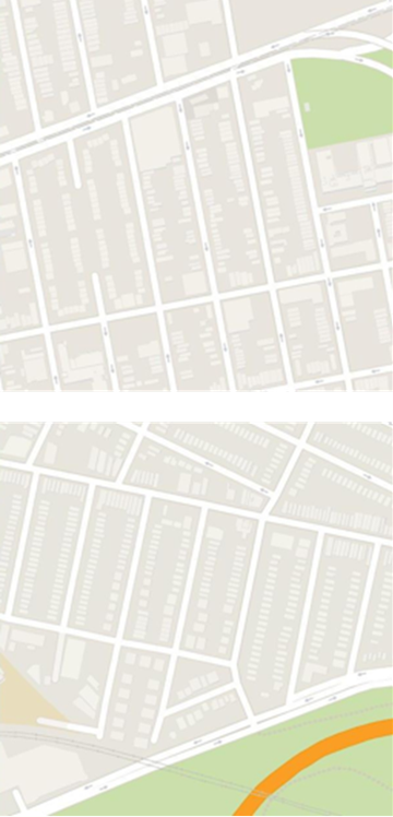
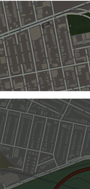
The results of the table clearly show the advantage of MTAdam over all baseline methods. In addition, it also shows a slight improvement in performance in comparison to the usage of Adam on the prescribed weights. Fig. 2 presents two representative samples from the facades test set. Pix2pix-Unbalanced introduces visual artifacts and suffers from mode collapse (it generates the same corrupted patch in the top right corner of many images). Pix2pix-Unbalanced-MTAdam yields higher-quality images, similar to those of the original Pix2Pix, using the prescribed weights.

Table 2: Comparing various methods for traning pix2pix. Lower is better for all metrics.

	Facade images				maps$\rightarrow$aerial
	L1	L2	NMSE	FID	L1	L2	NMSE	FID
Unbalanced-SGD-Momentum	120.12	18308	1.132	339.40	45.1	3428.3	0.491	102.45
Unbalanced-RMSProp	53.98	4913	0.303	136.10	42.4	3056.7	0.435	95.74
Unbalanced-Adam	54.92	5074	0.313	133.55	38.1	2632.3	0.368	88.08
Unbalanced-MTAdam	46.50	3822	0.236	130.38	33.6	2096.9	0.293	86.40
Hyperband-FID	54.12	4992	0.308	141.96	35.14	2391.2	0.341	86.45
Balanced-Adam	45.84	3811	0.235	130.50	34.4	2163.4	0.303	85.76

CycleGAN experiments

The CycleGAN objective function is composed of six loss terms:

$$\pazocal{L}_{CycleGAN}=\lambda_{1}\pazocal{L}_{GAN\_A}+\lambda_{1}\pazocal{L}_{GAN\_B}+\lambda_{2}\pazocal{L}_{cycle\_A}+\lambda_{2}\pazocal{L}_{cycle\_B}+\lambda_{3}\pazocal{L}_{idt\_A}+\lambda_{3}\pazocal{L}_{idt\_B}$$ (2)

Where the $\pazocal{L}_{GAN}$, $\pazocal{L}_{cycle}$, $\pazocal{L}_{idt}$ terms are the GAN loss, cycle GAN loss and identity loss, for each one of the sides (A or B). $\lambda_{1}$, $\lambda_{2}$ and $\lambda_{3}$ are set to 1, 10 and 0.5, respectively. In our experiments, we unbalance CycleGAN, by setting $\lambda_{2}$ to 1000, leaving $\lambda_{1}$ and $\lambda_{3}$ unchanged.

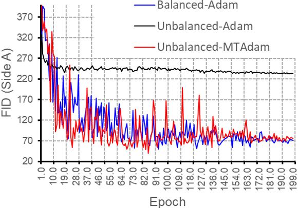
Fig. 3 compares the convergence of three CycleGAN models: unbalanced MTAdam, unbalanced Adam, and balanced Adam. All models are applied on the horse2zebra dataset [3]. As can be seen, MTAdam exhibits a competitive convergence to the Adam experiment applied with balanced weighting, which is much better than the performance of Adam on the unbalanced weights. Tab. 3 presents the performance of MTAdam applied on CycleGAN, compared to all five baselines, and evaluated on two datasets. MTAdam with an unbalanced initialization yields competitive performance to the Adam method, which uses the prescribed hyperparams.

Figure 3: The L1 (left) and FID (right) metrics evaluated per epoch CycleGAN models trained on the horse2zebra dataset [3]. (top) generated zebra images. (bottom) generated horse images.

Table 3: Performance of the various optimization methods, when applied to the CycleGAN algorithm.

		L1-A	L2-A	NMSE-A	FID-A	L1-B	L2-B	NMSE-B	FID-B
horse$\rightarrow$zebra	Unbalanced-SGD-Momentum	82.3	10217	0.5866	283.3	127.0	20331	0.9898	406.3
	Unbalanced-RMSProp	73.8	8384	0.4814	233.9	70.6	7683	0.3740	230.9
	Unbalanced-Adam	74.4	8421	0.4935	229.6	72.3	7742	0.3842	227.1
	Unbalanced-MTAdam	68.7	7235	0.4151	73.0	69.0	7281	0.3545	139.7
	Hyperband-FID	72.3	8049	0.4687	189.2	71.8	7584	0.3746	192.6
	Balanced-Adam	68.6	7248	0.4161	70.6	68.6	7207	0.3509	143.8
maps$\rightarrow$aerial	Unbalanced-SGD-Momentum	26.7	1102	0.0209	437.5	73.01	7146	1.0	738.6
	Unbalanced-RMSProp	12.9	389	0.0074	170.2	36.81	2260	0.3154	231.3
	Unbalanced-Adam	12.9	386	0.0073	166.3	37.00	2270	0.3161	234.2
	Unbalanced-MTAdam	10.6	376	0.0071	113.0	35.37	2242	0.3137	48.8
	Hyperband-FID	12.9	387	0.0073	169.4	36.91	2226	0.3102	233.1
	Balanced-Adam	8.5	301	0.0057	116.1	35.45	2250	0.3148	46.8

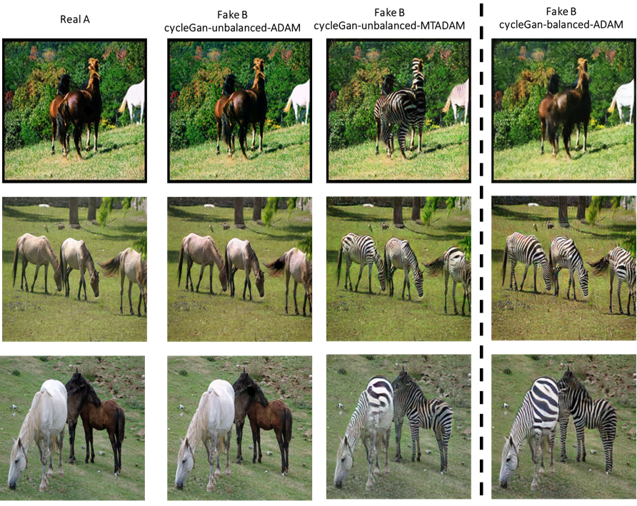
Fig. 4 exhibits representative images from the CycleGAN models, showing that MTAdam, even when applied to a loss with unbalanced weights, matches the results of Adams on the prescribed weights.

(a)	(b)	(c)	(d)	(e)

Figure 4: CycleGAN results for mapping (a) real maps to fake images in the aerial photos domain for (b) unbalanced Adam, (c) unbalanced MTAdam and (d) balanced Adam. (e) is the ground truth.

SRGAN  In the Super Resolution GAN (SRGAN) [14], the objective function is:

$$\pazocal{L}_{SRGAN}=\lambda_{1}\pazocal{L}_{MSE}+\lambda_{2}\pazocal{L}_{GAN}+\lambda_{3}\pazocal{L}_{Perceptual}$$ (3)

for which the total loss is a combination of a GAN loss, perceptual loss and MSE. The $\lambda_{1}$, $\lambda_{2}$ and $\lambda_{3}$ are set to 1, 0.001, 0.006. We unbalance SRGAN experiments by setting both $\lambda_{2}$ and $\lambda_{3}$ to 1 (i.e. applying all three terms with the same coefficient).

We evaluate SRGAN-Unbalanced-MTAdam on two test sets, Set14 [28] and BSD100[17]. The results, listed in Tab. 5 demonstrate that MTAdam can effectively recover from unbalanced weights, while the other optimization methods suffer a degradation in performance.

Table 4: SRGAN results. Higher is better for PSNR and SSIM. Lower is better for FID.

	Set14			BSD100
	PNSR	SSIM	FID	PSNR	SSIM	FID
Unbalanced-SGD-Momentum	22.95	0.6213	74.92	23.01	0.5997	79.45
Unbalanced-RMSProp	23.04	0.6252	72.92	23.14	0.6020	76.64
Unbalanced-Adam	23.43	0.6264	69.96	23.71	0.6070	77.24
Unbalanced-MTAdam	25.97	0.7219	66.03	25.23	0.6690	74.97
Hyperband-FID	24.89	66.24	67.26	24.80	0.6554	75.65
Balanced-Adam	26.02	0.7397	66.59	25.16	0.6688	72.57

Table 5: Ablation study results.

		pix2pix facade				CycleGAN horse2zebra
		L1	L2	NMSE	FID	L1-A	FID-A	L1-B	FID-B
(i)	Removing L6–8	53.45	5021	0.326	134.0	74.7	225.2	71.2	217.1
(ii)	Removing L6, changing $g^{i}_{\ell}$ to $g^{i}$	46.8	3850	0.258	133.5	70.1	75.2	69.5	145.7
(iii)	No scaling by $n_{\ell,t}^{1}$ in L8	46.7	3862	0.242	136.3	72.3	82.4	70.6	167.2
(iv)	Line 14: Scaling like Adam	48.2	3956	0.245	171.5	73.5	210.5	71.1	190.3
(v)	Line 14: scaling by mean instead of max	48.3	4020	0.249	156.8	73.7	208.4	71.6	173.5
	Full method	46.5	3822	0.236	130.4	68.7	73.0	69.0	139.7

4.3 Ablation Study

Tab. 5 presents an ablation study for unbalanced pix2pix on the facade images and for unbalanced CycleGAN on the zebra2horse dataset. The following variants are considered (the descriptions refer to Alg. 1): (i) treating all layers as one layer and eliminating lines 6-8 altogether. (ii) training all layers at one, and performing the normalization in line 8 once for the entire gradient, i.e., still normalizing by the magnitude of the gradient of the first term. (iii) scaling the gradients of each layer $l$ and each term $i$ in line 8 by $(n_{l,t}^{i})^{-1}$ but not by $n_{l,t}^{1}$. (iv) replacing the term ${\max(\widehat{v^{1}_{t}}...\widehat{v^{I}_{t}})}$ in line 14 with ${\widehat{v^{i}_{t}}}$, in an analog way to line 14 in Adam. (v) replacing the same term with the mean $I^{-1}\sum\widehat{v^{i}_{t}}$.

The results, shown in Tab. 5, indicate that it is crucial to employ a per layer analysis, in the way it is done in MTAdam, that normalizing by the magnitude of the gradient of an anchor term is highly beneficial, and that the maximal variance is a better alternative to alternative scaling terms.

5 Conclusions

MTAdam is shown to be a widely applicable optimizer, which can dynamically balance multiple loss terms in an effective way. While tested on image generation tasks, it is a general algorithm, which can find its usage in other types of tasks that require the optimization of multiple terms, such as domain adaptation and some forms of self-supervised learning. Our code can be found here. MTAdam is implemented as a generic pytorch optimizer and applying it is almost as simple as applying Adam.

Appendix

Appendix A Image synthesis samples

Fig. 5 presents a few representative samples from the CycleGAN[29] experiments, employed to transfer horse images to zebras. As can be seen, the unbalanced Adam training completely fails to generate zebras images and collapses to the identity mapping. This can be attributed to the domination of cyclic loss in the unbalanced settings, which dictates the convergence, leaveing the other loss terms ineffective. On the other hand, the unbalanced MTAdam model was able to successfully generate zebra images, in a quality that is similar or better to the balanced adam model (which uses the prescribed weights). In particular, in the first row, we can see that CycleGAN-Unbalanced-MTAdam was able to outperform the CycleGAN-Balanced-Adam experiment, as the latter fails to generate a zebra image for this particular sample, while MTAdam was able to generate a fairly good quality image.

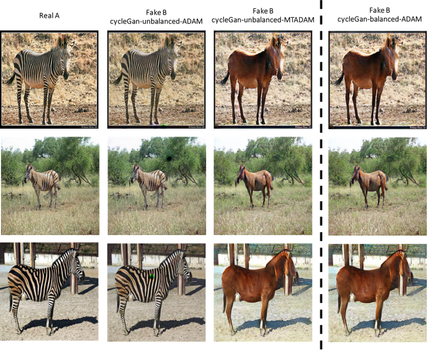
Fig. 6 depicts a few samples from the same models described above, this time employed to generate horse images from zebra images. As can be seen, the unbalanced Adam fails again to generate horse images, collapses to the identity mapping, and this time also introduces visual artifacts in a few images (see the green artifact in the bottom row). In addition, MTAdam yields images of the same quality as the balanced Adam experiment.

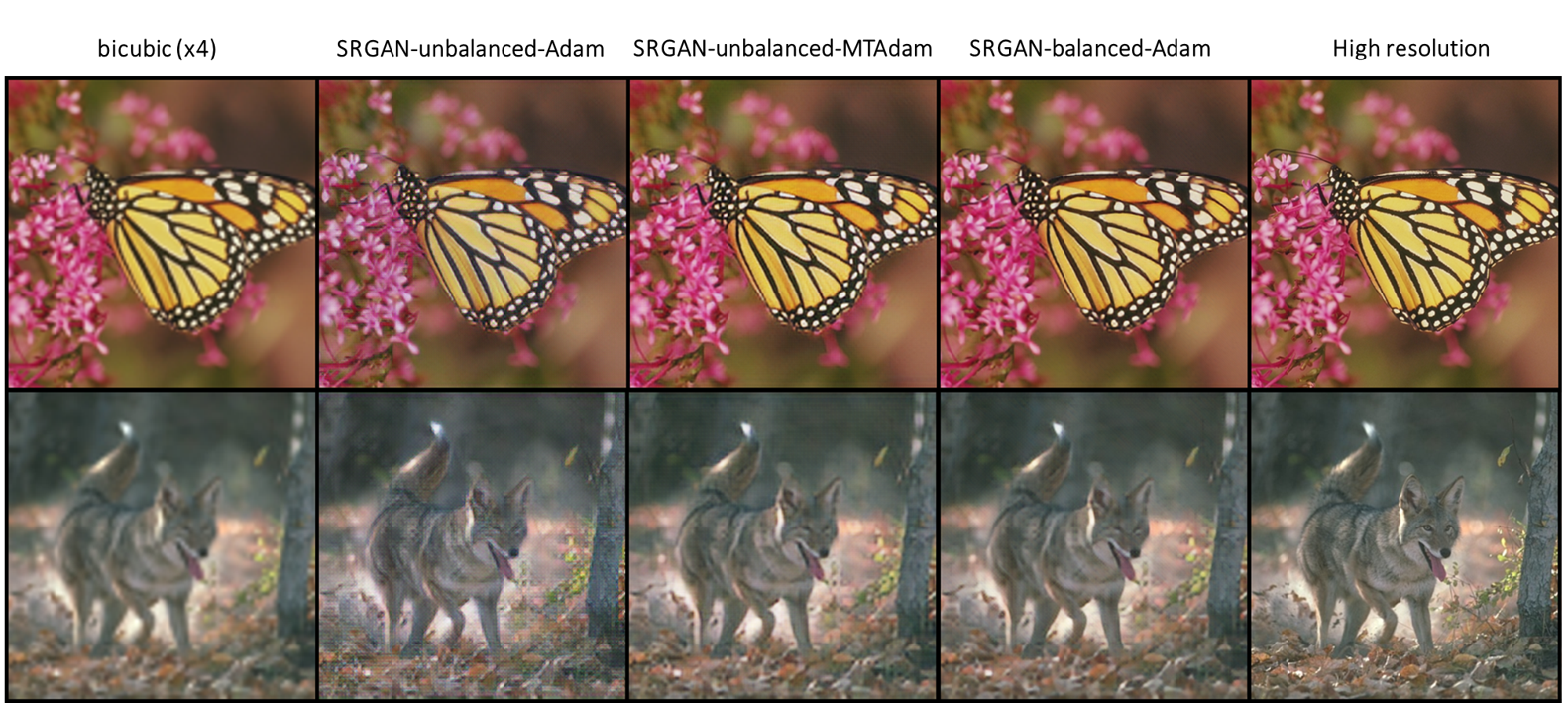
Fig. 7 presents visual results for the SRGAN [14] experiments. The images were taken from Set14 [28]. All models were trained to generate high-resolution images from low-resolution images, with a factor of 4x upscaling. As can be seen, the SRGAN model that employs unbalanced weights and Adam optimizer yields images with visual artifacts, and low fidelity. This can be attributed to the domination of the GAN and perceptual loss terms over the pixel-wise term. In contrast, the SRGAN model that employs our MTAdam optimizer with unbalanced weights yields images of the same quality as the SRGAN that utilizes the prescribed weights [14] and Adam.

Figure 5: Samples from the CycleGAN experiments employed on the zebra2horse dataset, mapping horse images to zebras. CycleGAN-Balanced-Adam employs CycleGAN with the prescribed weights [29]. CycleGAN-Unbalanced-Adam runs with unbalanced initial weights, which fails to generate zebra images. CycleGAN-Unbalanced-MTAdam (our method) starts with unbalanced weights but produces images of the same quality as CycleGAN-Balanced-Adam.

Figure 6: Samples from the CycleGAN experiments employed on the zebra2horse dataset, mapping zebra images to horses. CycleGAN-Balanced-Adam employs CycleGAN with the prescribed weights [29]. CycleGAN-Unbalanced-Adam runs with unbalanced initial weights, fails to generate horse images, collapses to identity mapping, and introduces visual artifacts. CycleGAN-Unbalanced-MTAdam (our method) starts with unbalanced weights but produces images of the same quality as CycleGAN-Balanced-Adam.

Figure 7: Samples from the test set of the SRGAN[14] experiments. Images were taken from Set14[28]. SRGAN-Unbalaced-Adam employs SRGAN training with the unbalanced initial weights, as described in the main text. SRGAN-Balanced-Adam employs SRGAN with the prescribed weights. SRGAN-Unbalanced-MTAdam utilizes our proposed MTAdam optimizer, runs with unbalanced initial weights but produces images of the same quality of SRGAN-Balanced-Adam.

References

- [1] James S Bergstra, Rémi Bardenet, Yoshua Bengio, and Balázs Kégl. Algorithms for hyper-parameter optimization. In Advances in neural information processing systems, pages 2546–2554, 2011.
- [2] Rich Caruana. Multitask learning. Machine learning, 28(1):41–75, 1997.
- [3] Jia Deng, Wei Dong, Richard Socher, Li-Jia Li, Kai Li, and Li Fei-Fei. Imagenet: A large-scale hierarchical image database. In 2009 IEEE conference on computer vision and pattern recognition, pages 248–255. Ieee, 2009.
- [4] Long Duong, Trevor Cohn, Steven Bird, and Paul Cook. Low resource dependency parsing: Cross-lingual parameter sharing in a neural network parser. In Proceedings of the 53rd Annual Meeting of the Association for Computational Linguistics and the 7th International Joint Conference on Natural Language Processing (Volume 2: Short Papers), pages 845–850, 2015.
- [5] Matthias Feurer, Jost Tobias Springenberg, and Frank Hutter. Using meta-learning to initialize bayesian optimization of hyperparameters. In Proceedings of the 2014 International Conference on Meta-learning and Algorithm Selection-Volume 1201, pages 3–10. Citeseer, 2014.
- [6] Ian Goodfellow, Jean Pouget-Abadie, Mehdi Mirza, Bing Xu, David Warde-Farley, Sherjil Ozair, Aaron Courville, and Yoshua Bengio. Generative adversarial nets. In Advances in Neural Information Processing Systems 27, pages 2672–2680. 2014.
- [7] Kaiming He, Georgia Gkioxari, Piotr Dollár, and Ross Girshick. Mask r-cnn. In Proceedings of the IEEE international conference on computer vision, pages 2961–2969, 2017.
- [8] Martin Heusel, Hubert Ramsauer, Thomas Unterthiner, Bernhard Nessler, and Sepp Hochreiter. Gans trained by a two time-scale update rule converge to a local nash equilibrium. In Advances in neural information processing systems, pages 6626–6637, 2017.
- [9] Frank Hutter, Holger H Hoos, and Kevin Leyton-Brown. Sequential model-based optimization for general algorithm configuration. In International conference on learning and intelligent optimization, pages 507–523. Springer, 2011.
- [10] Phillip Isola, Jun-Yan Zhu, Tinghui Zhou, and Alexei A Efros. Image-to-image translation with conditional adversarial networks. In Proceedings of the IEEE conference on computer vision and pattern recognition, pages 1125–1134, 2017.
- [11] Justin Johnson, Alexandre Alahi, and Li Fei-Fei. Perceptual losses for real-time style transfer and super-resolution. In European conference on computer vision, pages 694–711. Springer, 2016.
- [12] Alex Kendall, Yarin Gal, and Roberto Cipolla. Multi-task learning using uncertainty to weigh losses for scene geometry and semantics. In Proceedings of the IEEE conference on computer vision and pattern recognition, pages 7482–7491, 2018.
- [13] Diederik P Kingma and Jimmy Ba. Adam: A method for stochastic optimization. arXiv preprint arXiv:1412.6980, 2014.
- [14] Christian Ledig, Lucas Theis, Ferenc Huszár, Jose Caballero, Andrew Cunningham, Alejandro Acosta, Andrew Aitken, Alykhan Tejani, Johannes Totz, Zehan Wang, et al. Photo-realistic single image super-resolution using a generative adversarial network. In Proceedings of the IEEE conference on computer vision and pattern recognition, pages 4681–4690, 2017.
- [15] Lisha Li, Kevin Jamieson, Giulia DeSalvo, Afshin Rostamizadeh, and Ameet Talwalkar. Hyperband: A novel bandit-based approach to hyperparameter optimization. The Journal of Machine Learning Research, 18(1):6765–6816, 2017.
- [16] Mingsheng Long and Jianmin Wang. Learning multiple tasks with deep relationship networks. arXiv preprint arXiv:1506.02117, 2:1, 2015.
- [17] David Martin, Charless Fowlkes, Doron Tal, and Jitendra Malik. A database of human segmented natural images and its application to evaluating segmentation algorithms and measuring ecological statistics. In Proceedings Eighth IEEE International Conference on Computer Vision. ICCV 2001, volume 2, pages 416–423. IEEE, 2001.
- [18] Lars Mescheder, Sebastian Nowozin, and Andreas Geiger. The numerics of gans. In Advances in Neural Information Processing Systems, pages 1825–1835, 2017.
- [19] Shaoqing Ren, Kaiming He, Ross Girshick, and Jian Sun. Faster r-cnn: Towards real-time object detection with region proposal networks. In Advances in neural information processing systems, pages 91–99, 2015.
- [20] David E Rumelhart, Geoffrey E Hinton, and Ronald J Williams. Learning representations by back-propagating errors. nature, 323(6088):533–536, 1986.
- [21] Jasper Snoek, Hugo Larochelle, and Ryan P Adams. Practical bayesian optimization of machine learning algorithms. In Advances in neural information processing systems, pages 2951–2959, 2012.
- [22] Niranjan Srinivas, Andreas Krause, Sham M Kakade, and Matthias Seeger. Gaussian process optimization in the bandit setting: No regret and experimental design. arXiv preprint arXiv:0912.3995, 2009.
- [23] T. Tieleman and G. Hinton. Lecture 6.5—RmsProp: Divide the gradient by a running average of its recent magnitude. COURSERA: Neural Networks for Machine Learning, 2012.
- [24] Radim Tyleček and Radim Šára. Spatial pattern templates for recognition of objects with regular structure. In German Conference on Pattern Recognition, pages 364–374. Springer, 2013.
- [25] Zhou Wang, Alan C Bovik, Hamid R Sheikh, and Eero P Simoncelli. Image quality assessment: from error visibility to structural similarity. IEEE transactions on image processing, 13(4):600–612, 2004.
- [26] Zi Wang, Bolei Zhou, and Stefanie Jegelka. Optimization as estimation with gaussian processes in bandit settings. In Artificial Intelligence and Statistics, pages 1022–1031, 2016.
- [27] Yongxin Yang and Timothy M Hospedales. Trace norm regularised deep multi-task learning. arXiv preprint arXiv:1606.04038, 2016.
- [28] Roman Zeyde, Michael Elad, and Matan Protter. On single image scale-up using sparse-representations. In International conference on curves and surfaces, pages 711–730. Springer, 2010.
- [29] Jun-Yan Zhu, Taesung Park, Phillip Isola, and Alexei A Efros. Unpaired image-to-image translation using cycle-consistent adversarial networks. In Proceedings of the IEEE international conference on computer vision, pages 2223–2232, 2017.