The high energy window of probing dark matter with cosmic-ray antideuterium and antihelium

Abstract

Cosmic-ray (CR) anti-nuclei are often considered as important observables for dark matter (DM) indirect detections at low kinetic energies below GeV per nucleon. Since the primary CR fluxes drop quickly towards high energies, the secondary anti-nuclei in CR are expected to be significantly suppressed in high energy regions ($\gtrsim 100$ GeV per nucleon). If DM particles are heavy, the annihilation productions of DM can be highly boosted, thus the fluxes of anti-nuclei produced by DM annihilations may exceed the secondary background at high energies, which opens a high energy window for DM indirect detections. We investigate the possibility of detecting heavy DM particles which annihilate into high energy anti-nuclei. We use Monte-Carlo generators PYTHIA, EPOS-LHC and DPMJET and the coalescence model to simulate the production of anti-nuclei, and constrain the DM annihilation cross sections by using the AMS-02 and HAWC antiproton data and the HESS galactic center gamma-ray data. We find that the conclusion depends on the choice of DM density profiles. For the “Cored” type profile with a DM particle mass $\gtrsim 10$ TeV, the contributions from DM annihilations can exceed the secondary background in high energy regions, which opens the high energy window. While for the “Cuspy” type profile, the excess disappears.
Keywords: dark matter, coalescence model, antideuterium, antihelium
ArXiv ePrint: 2006.14681

I Introduction

The existence of dark matter (DM) is supported by various astronomic observations at different scales, but the particle nature of DM is still mysterious. As an important probe in DM indirect detections, the antiparticles in cosmic rays (CR) may shed light on the properties of DM. In recent years, a number of experiments have shown an unexpected structure in the CR positron data Beatty:2004cy ; Adriani:2008zr ; FermiLAT:2011ab ; Accardo:2014lma , which could be related to the DM annihilation or decay Kopp:2013eka ; Bergstrom:2013jra ; Ibarra:2013zia ; Jin:2013nta . Unlike CR positrons, the CR antiproton flux data from PAMELA Adriani:2012paa , BESS-polar II Abe:2011nx and AMS-02 Aguilar:2016kjl do not show significant discrepancies with the secondary production of antiproton, and these null results can be used to place stringent constraints on the DM annihilation cross sections Giesen:2015ufa ; Jin:2015sqa ; Lin:2016ezz ; Reinert:2017aga .

CR heavy anti-nuclei such as antideuterium ($\overline{\text{D}}$) and antihelium-3 (${}^{3}\overline{\text{He}}$) are supposed to be important probes for the DM Donato:1999gy ; Carlson:2014ssa ; Cirelli:2014qia . The $\overline{\text{D}}$ and ${}^{3}\overline{\text{He}}$ in CR can be generated as secondary productions by the collisions between the primary CR particles and the interstellar gas, or they can be produced by the DM annihilation or decay. However, the secondary $\overline{\text{D}}$ and ${}^{3}\overline{\text{He}}$ are boosted to high kinetic energies because of the high production threshold in $pp$-collisions (17$m_{p}$ for $\overline{\textrm{D}}$ and 31$m_{p}$ for ${}^{3}\overline{\text{He}}$, where $m_{p}$ is the proton mass), thus the signal from DM can be distinguished in low energy regions (below GeV per nucleon). Although the fluxes of anti-nuclei decrease rapidly with the increase of the atom mass number $A$, the high signal-to-background ratio at low energies and the experiments with high sensitivities (such as AMS-02 Giovacchini:2007dwa ; Kounine:2010js and GAPS Aramaki:2015laa ) make it possible to distinguish the contributions originated from DM interactions. Furthermore, an advantage for considering $\overline{\text{D}}$ and ${}^{3}\overline{\text{He}}$ is that their productions are highly correlated with CR antiprotons, the uncertainties of the $\overline{\text{D}}$ and ${}^{3}\overline{\text{He}}$ fluxes can be greatly reduced by the CR $\bar{p}$ data Li:2018dxj .

In the literature (for a recent review, see Ref. vonDoetinchem:2020vbj ), the analysis of the DM produced $\overline{\text{D}}$ and ${}^{3}\overline{\text{He}}$ are focused on the low kinetic energy regions, which we refer as the low energy window. In our previous analysis Li:2018dxj , we have studied the prospects of detecting DM through the low energy antihelium. We systematically analysed the uncertainties from propagation models, DM density profiles and MC generators, and reduced the uncertainties by constraining the DM annihilation cross sections with the AMS-02 $\bar{p}/p$ data. However, the low energy window suffers from the uncertainties of solar activities (solar modulations). In this work, we investigate the possibility of probing DM with high energy CR $\overline{\text{D}}$ and ${}^{3}\overline{\text{He}}$ particles. In high energy regions (typically above 100 GeV per nucleon), the flux of primary CR particles drops quickly (the flux of CR proton is proportional to $E^{-2.75}$), which leads to a suppression on the high energy secondary CR particles. As a result, the fluxes of anti-nuclei produced by DM annihilations may exceed the secondary background and open a high energy window for probing the DM.

We use the Monte-Carlo (MC) event generators PYTHIA 8.2 Sjostrand:2006za ; Sjostrand:2014zea , EPOS-LHC Werner:2005jf ; Pierog:2013ria and DPMJET-III Roesler:2001mn to fit the coalescence momenta for anti-nuclei with the experiments including ALEPH Schael:2006fd , CERN ISR Henning:1977mt and ALICE Acharya:2017fvb , and generate the energy spectra of anti-nuclei. The propagation of CR particles are calculated by using the GALPROP code. We use the AMS-02 Aguilar:2016kjl and HAWC $\bar{p}/p$ data Abeysekara:2018syp and the HESS galactic center (GC) $\gamma$-ray data Abramowski:2011hc ; Abdallah:2016ygi to constrain the DM annihilation cross sections. We find that the conclusion is depend on the choice of DM density profiles. For a large DM mass ($\gtrsim 10$ TeV) with the relatively flat “Cored” type DM profile, the high energy window exist. While for a typical steep DM profile like “Cuspy” type, the high energy window closes.

This paper is organized as follows: In section II, we briefly review the coalescence model and determine the coalescence momenta for anti-nuclei by fitting the ALEPH, ALICE and CERN-ISR data. In section III, we review the theory of CR propagation. In section IV, we constrain the DM annihilation cross section by using the $\bar{p}/p$ data from AMS-02 and HAWC and $\gamma-$ray data from HESS. The fluxes of $\overline{\text{D}}$ and ${}^{3}\overline{\text{He}}$ for DM direct annihilation and annihilation through mediator channels are presented in section V. The conclusions are summarized in section VI.

II The coalescence model and coalescence momenta

The formation of anti-nuclei can be described by the coalescence model Butler:1963pp ; Schwarzschild:1963zz ; Csernai:1986qf , which uses a single parameter, the coalescence momentum $p_{0}^{\scriptscriptstyle\bar{\mathrm{A}}}$ to quantify the probability of anti-nucleons merge into an anti-nucleus $\bar{\mathrm{A}}$. The basic idea of this model is that anti-nucleons combine into an anti-nucleus if the relative four-momenta of a proper set of nucleons is less than the coalescence momentum. For example, the coalescence criterion for $\overline{\text{D}}$ is written as:

$$||k_{\bar{p}}-k_{\bar{n}}||=\sqrt{(\Delta\vec{k})^{2}-(\Delta E)^{2}}<p_{0}^{\scriptscriptstyle\overline{\mathrm{D}}},$$ (1)

where $k_{\bar{p}}$ and $k_{\bar{n}}$ are the four-momenta of antiproton and antineutron respectively, and $p_{0}^{\bar{\scriptscriptstyle\mathrm{D}}}$ is the coalescence momentum of $\overline{\text{D}}$. If we assume that the momenta distribution of the $\bar{p}$ and $\bar{n}$ in one collision event are uncorrelated and isotropic, the spectrum of $\overline{\text{D}}$ can be derived by the phase-space analysis:

$$\gamma_{\bar{\scriptscriptstyle\mathrm{D}}}\frac{d^{3}N_{\bar{\scriptscriptstyle\mathrm{D}}}}{d^{3}\vec{k}_{\bar{\scriptscriptstyle\mathrm{D}}}}(\vec{k}_{\bar{\scriptscriptstyle\mathrm{D}}})=\frac{\pi}{6}\left(p_{0}^{\bar{\scriptscriptstyle\mathrm{D}}}\right)^{3}\cdot\gamma_{\bar{p}}\frac{d^{3}N_{\bar{p}}}{d^{3}\vec{k}_{\bar{p}}}(\vec{k}_{\bar{p}})\cdot\gamma_{\bar{n}}\frac{d^{3}N_{\bar{n}}}{d^{3}\vec{k}_{\bar{n}}}(\vec{k}_{\bar{n}}),$$ (2)

where $\gamma_{\bar{\scriptscriptstyle\mathrm{D}},\bar{p},\bar{n}}$ are the Lorentz factors, and $\vec{k}_{\bar{p}}\approx\vec{k}_{\bar{n}}\approx\vec{k}_{\bar{\scriptscriptstyle\mathrm{D}}}/2$.

For ${}^{3}\overline{\text{He}}$, we adopt the same coalescence criterion as in our previous analysis Li:2018dxj . We compose a triangle using the norms of the three relative four-momenta $l_{1}=||k_{1}-k_{2}||,~{}~{}l_{2}=||k_{2}-k_{3}||$ and $l_{3}=||k_{1}-k_{3}||$, where $k_{1},k_{2},k_{3}$ are the four-momenta of the three anti-nucleons respectively. And then, making a circle with minimal diameter to envelop the triangle, if the diameter of this circle is smaller than $p_{0}^{\scriptscriptstyle\overline{\mathrm{He}}}$, an ${}^{3}\overline{\text{He}}$ is generated. If the triangle is acute, the minimal circle is just the circumcircle of this triangle, and the coalescence criterion can be expressed as follows:

$$d_{\mathrm{circ}}=\frac{l_{1}l_{2}l_{3}}{\sqrt{(l_{1}+l_{2}+l_{3})(-l_{1}+l_{2}+l_{3})(l_{1}-l_{2}+l_{3})(l_{1}+l_{2}-l_{3})}}<p_{0}^{\scriptscriptstyle\overline{\mathrm{He}}}.$$ (3)

Otherwise, the minimal diameter is equal to the longest side of the triangle, and the criterion can be simply written as $\text{max}\{l_{1},l_{2},l_{3}\}<p_{0}^{\scriptscriptstyle\overline{\mathrm{He}}}$. See Ref. Li:2018dxj for more details.

We use the MC generators PYTHIA 8.2, EPOS-LHC and DPMJET-III to simulate the hadronization after DM annihilations and $pp-$collisions, and then adopt the coalescence model to produce anti-nuclei form the final state $\bar{p}$ or $\bar{n}$. The spatial distance between each pair of anti-nucleons also needs to be considered, because anti-nucleons should be close enough to under go the nuclear reactions and then merge into anti-nuclei. We set all the particles with lifetime $\tau\gtrsim 2\,\,\mathrm{fm}/c$ to be stable to ensure that every pair of anti-nucleons are located in a short enough distance Carlson:2014ssa , where 2 fm is approximately the size of the ${}^{3}\overline{\textrm{He}}$ nucleus.

The value of coalescence momenta should be determined by the experimental data, which are often released in the form of coalescence parameters $B_{A}$. The definition of the coalescence parameter $B_{A}$ is expressed by the formula:

$$E_{A}\frac{d^{3}N_{A}}{dp_{A}^{3}}=B_{A}\left(E_{p}\frac{d^{3}N_{p}}{dp_{p}^{3}}\right)^{Z}\left(E_{n}\frac{d^{3}N_{n}}{dp_{n}^{3}}\right)^{N},\ \ \ \vec{p}_{p}=\vec{p}_{n}=\vec{p}_{A}/A,$$ (4)

where $A=Z+N$ is the mass number of the nucleus, $Z$ and $N$ are the proton number and the neutron number respectively. Under the assumption that the momenta distribution of the $\bar{p}$ and $\bar{n}$ are uncorrelated and isotropic, the relation $B_{A}\propto p_{0}^{3(A-1)}$ is expected by comparing Eq. (2) and Eq. (4). However, the jet structure and the correlation between $\bar{p}$ and $\bar{n}$ play important roles in the formation of anti-nuclei. So we derive the coalescence momenta by using the MC generators to fit the experimental data, thus the effect of jet structures and correlations are included.

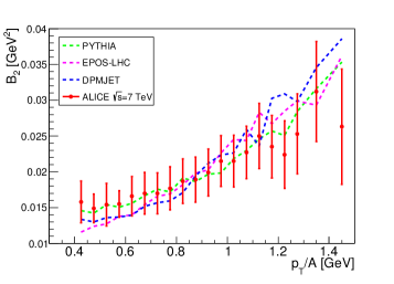
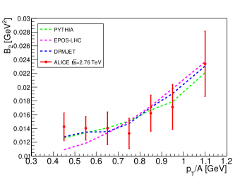
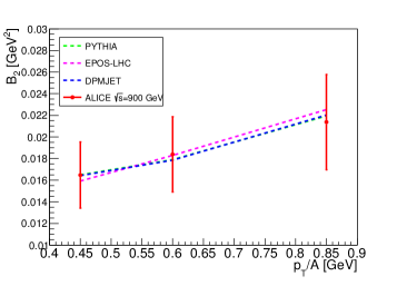
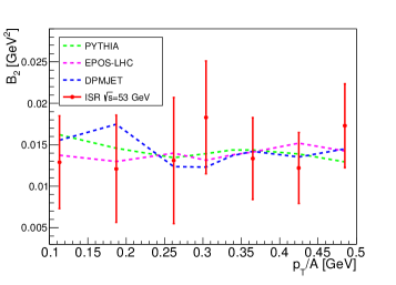
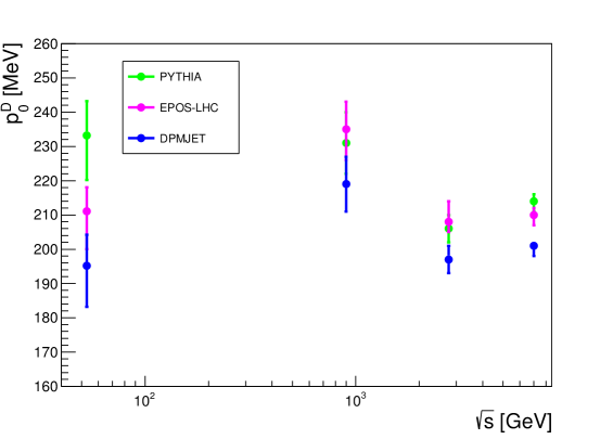
To derive the coalescence momentum of $\overline{\mathrm{D}}$ in $pp$ collisions, we follow the procedures described in Ref. Li:2018dxj to fit the coalescence parameter $B_{2}$ data from the ALICE-7 TeV, 2.76 TeV, 900 GeV Acharya:2017fvb and ISR-53 GeV Henning:1977mt experiments. We use MC generators to simulate these experiments, and record the momenta information of $\bar{p}$, $\bar{n}$ that are possible to form a $\overline{\mathrm{D}}$. We select the $\bar{p}$ and $\bar{n}$ according to a sufficiently large coalescence momentum $p_{0,\text{max}}$ (600 MeV for $\overline{\mathrm{D}}$, 1 GeV for $\overline{\mathrm{He}}$), and then calculate the spectra of $\overline{\text{D}}$ for different $p_{0}^{\scriptscriptstyle\overline{\mathrm{D}}}$ values that are smaller than $p_{0,\text{max}}$. The $B_{2}$ values are calculated by using the Eq. (4), and we make a $\chi^{2}$ analysis to find the value of $p_{0}^{\scriptscriptstyle\overline{\mathrm{D}}}$. The best-fit $B_{2}$ values are shown in Fig. 1. We find $\chi^{2}_{\text{min}}/\text{d.o.f}<1$ for all these fits, which means the fitting results are in good agreement with the experimental data. As shown by the figure, the $p_{T}$-dependence are well reproduced by the coalescence model and the MC generators.

The fitting result of $p_{0}^{\scriptscriptstyle\overline{\mathrm{D}}}$ are listed in Tab. 1, and the values in brackets are the results given by ALICE group, which are only available for ALICE 7 TeV and ISR-53 GeV experiments with PYTHIA 8.2 and EPOS-LHC generators. We can see that for ALICE 7 TeV, our best-fit values are in good agreements with the ones from ALICE group, but for ISR-53 GeV, our results are larger. This is partially because ALICE group have only generated the energy spectra of $\overline{\text{D}}$ for six $p_{0}^{\scriptscriptstyle\overline{\mathrm{D}}}$ values Acharya:2017fvb , and used the isotropic approximation $B_{A}\approx p_{0}^{3(A-1)}$ to interpolate the spectra for other $p_{0}^{\scriptscriptstyle\overline{\mathrm{D}}}$ values, while we generate the $\overline{\text{D}}$ spectra for every integer number MeV and do not need the approximation. Moreover, in fitting the ISR-53 GeV experiment, ALICE group have manually rescaled the spectra of $\bar{p}$ generated by MC to better reproduce the experimental data, while we do not make this correction for self-consistencies.

FIG. 1: The best-fit $B_{2}$ values from MC generators compare with the ALICE Acharya:2017fvb and CERN-ISR Henning:1977mt $pp$-collision data. $topleft)$ ALICE-7 TeV, $topright)$ ALICE-2.76 TeV, $bottomleft)$ ALICE-900 GeV, $bottomright)$ ISR-53 GeV.

FIG. 2: The $p_{0}$ values of ${\overline{\mathrm{D}}}$ from fitting the $pp$-collision data with three MC generators.

MC generators	ALICE 7 TeV	ALICE 2.76 TeV	ALICE 900 GeV	ISR 53 GeV
PYTHIA 8.2	$214^{+2}_{-3}~{}(216\pm 8)$	$206^{+4}_{-4}$	$231^{+9}_{-9}$	$233^{+10}_{-13}~{}(188\pm 8)$
EPOS-LHC	$210^{+2}_{-3}~{}(200\pm 10)$	$208^{+6}_{-3}$	$235^{+8}_{-9}$	$211^{+7}_{-11}~{}(190\pm 8)$
DPMJET-III	$201^{+1}_{-3}$	$197^{+4}_{-4}$	$219^{+8}_{-8}$	$195^{+9}_{-12}$

TAB. 1: Best-fit values of $p_{0}^{\overline{\mathrm{D}}}$ in unit of MeV, derived by fitting the $pp$-collision data with three MC generators PYTHIA 8.2 Sjostrand:2006za ; Sjostrand:2014zea , EPOS-LHC Werner:2005jf ; Pierog:2013ria and DPMJET-III Roesler:2001mn . The $p_{0}^{\overline{\mathrm{D}}}$ values do not show a clear relation with the $\sqrt{s}$ value of the experiments. The values in brackets are fitting results given by ALICE group.

In Fig. 2, we show the $p_{0}^{\scriptscriptstyle\overline{\mathrm{D}}}$ values for different $pp$ collision experiments with various MC generators. As can be seen, $p_{0}^{\scriptscriptstyle\overline{\mathrm{D}}}$ do not show a clear relation with the $\sqrt{s}$ values of the experiments. Since the fitting results for different center-of-mass energies are similar, we assume that the $p_{0}^{\overline{\mathrm{D}}}$ value does not vary with the $\sqrt{s}$ of the experiment. By fitting these $p_{0}^{\overline{\mathrm{D}}}$, we get $p_{0}^{\overline{\mathrm{D}}}(\texttt{PYTHIA)}=213\pm 2$ MeV, $p_{0}^{\overline{\mathrm{D}}}(\texttt{EPOS-LHC)}=211\pm 2$ MeV and $p_{0}^{\overline{\mathrm{D}}}(\texttt{DPMJET)}=201\pm 2$ MeV for $pp$-collisions.

By using PYTHIA 8.2  to fit the $B_{2}=3.3\pm 1.0\pm 0.8\times 10^{-3}$ data from the ALEPH $e^{+}e^{-}\rightarrow Z^{0}\rightarrow\overline{\mathrm{D}}$ experiment Schael:2006fd , we find $p_{0}^{\overline{\mathrm{D}}}(Z^{0})=190^{+23}_{-27}$ MeV. Considering the similarity between the dynamics of the $Z^{0}$ decay and the DM annihilation, we set $p_{0}^{\overline{\mathrm{D}}}(Z^{0})$ to be the coalescence momentum for the DM annihilations process $\chi\chi\rightarrow\overline{\mathrm{D}}+X$.

For ${}^{3}\overline{\text{He}}$, we adopt the $p_{0}^{\overline{\mathrm{He}}}$ value obtained in our previous work Li:2018dxj , which determining $p_{0}^{\overline{\mathrm{He}}}$ by fitting the ALICE $\sqrt{s}=7$ TeV $pp$-collision data, the results are listed in Tab. 2. Note that, ${}^{3}\overline{\text{He}}$ particles can be produced from two channels: direct formation from the coalescence of $\bar{p}\bar{p}\bar{n}$, or through the $\beta$-decay of an antitriton $\overline{\text{T}}$ ($\bar{p}\bar{n}\bar{n}$). The direct formation channel are suppressed by the Coulomb-repulsion between the two antiprotons, thus some previous works only considered the antitriton channel. However, our calculation shows that the direct formation channel are not negligible. The coalescence momentum of ${}^{3}\overline{\mathrm{He}}$ are only slightly smaller than that of $\overline{\text{T}}$, and the Gamow factor $\mathcal{G}\sim\exp(-2\pi\alpha m_{p}/p_{0}^{\overline{\mathrm{He}}})\approx 0.8$ Blum:2017qnn , these indicate that the Coulomb-repulsion may not be significant. By these facts, it is reasonable to ignore the Coulomb-repulsion in the MC simulation, and the contributions from both channels are included in this work. Our MC calculation shows that about $30\%$ of ${}^{3}\overline{\mathrm{He}}$ are produced through the direct formation channel. For the lack of the $e^{+}e^{-}\rightarrow^{3}\overline{\text{He}}$ experiments data, we set $p_{0}^{\overline{\mathrm{He}}/\overline{\mathrm{T}}}(\texttt{PYTHIA)}$ to be the coalescence momentum for the DM annihilation process $\chi\chi\rightarrow\overline{\mathrm{He}}/\overline{\mathrm{T}}+X$. It is known that the coalescence momentum varies for different processes and center of mass energies Aramaki:2015pii , and the relation $B_{A}\approx p_{0}^{3(A-1)}$ makes $p_{0}$ a crutial factor for the uncertainties of the final fluxes. In some previous analyses, the value of $p_{0}^{\overline{\mathrm{He}}}$ is estimated using various approaches, for example, by using the binding energy relation between $p_{0}^{\overline{\mathrm{He}}}$ and $p_{0}^{\overline{\mathrm{D}}}$ or assuming the ratio $p_{0}^{\overline{\mathrm{He}}}/p_{0}^{\overline{\mathrm{D}}}=p_{0}^{\mathrm{He}}/p_{0}^{\mathrm{D}}$ Carlson:2014ssa , and some works just set $p_{0}^{\overline{\mathrm{He}}}=p_{0}^{\overline{\mathrm{D}}}$  Cirelli:2014qia . The $p_{0}^{\overline{\mathrm{He}}}$ results from these approaches are different. It is worth mention that our $p_{0}^{\overline{\mathrm{He}}}$ value is relatively small comparing to previous works, which leads to conservative DM contributions.

MC generators:	PYTHIA 8.2	EPOS-LHC	DPMJET-III
$p_{0}^{\overline{\mathrm{He}}}$ (MeV)	$224^{+12}_{-16}$	$227^{+11}_{-16}$	$212^{+10}_{-13}$
$p_{0}^{\bar{\mathrm{T}}}$ (MeV)	$234^{+17}_{-29}$	$245^{+17}_{-30}$	$222^{+16}_{-26}$

TAB. 2: Best-fit values of $p_{0}^{\overline{\mathrm{He}}}$ and $p_{0}^{\bar{\mathrm{T}}}$ from Ref. Li:2018dxj , which is obtained by fitting the ALICE $pp$-collision data at $\sqrt{s}=7$ TeV for three MC generators PYTHIA 8.2, EPOS-LHC and DPMJET-III.

For the primary anti-particles originated from DM annihilations, the injection spectra are calculated using PYTHIA 8.2. We simulate the annihilation of Majorana DM particles by a positron-electron annihilation process $e^{+}e^{-}\rightarrow\phi^{*}\rightarrow f\bar{f}$, where $\phi^{*}$ is a fictitious scaler singlet and $f$ is a standard model final state. We set $\sqrt{s}=2m_{\chi}$ and switch off all initial-state-radiations in PYTHIA 8.2 to mimic the dynamics of DM annihilation. Three kinds of final states are considered: $q\bar{q}$ ($q$ stands for $u$ or $d$ quark), $b\bar{b}$ and $W^{+}W^{-}$. In EPOS-LHC and DPMJET-III generators, only hadrons can be set as the initial states, which do not resemble the properties of DM annihilations.

For the secondary anti-particles produced in $pp-$collisions, EPOS-LHC and DPMJET-III are used to generate the energy spectra. The default parameters in PYTHIA 8.2 (the Monash tune Skands:2014pea ) are focused to reproduce the experimental results at high center-of-mass energies (like ATLAS at $\sqrt{s}=7$ TeV Aad:2011gj ), but are not optimized for the energy regions around a few tens of GeV, which give the dominating contributions for the secondary CR anti-particles. To evaluate the performance of MC generators at low center-of-mass energies, we make a comparison between the $\bar{p}$ differential invariant cross section obtained by MC generators and the NA49 data at $\sqrt{s}=17.3$ GeV Anticic:2009wd . This comparison shows that EPOS-LHC has the best performance, DPMJET-III are also in relatively good agreements with the experiment, while the production cross section of $\bar{p}$ given by PYTHIA 8.2 are larger than the NA49 data roughly by a factor of two. In this paper, we will draw our conclusion based on the results from EPOS-LHC, and the difference between EPOS-LHC and DPMJET-III can be used as a rough estimation of the uncertainties from different MC generators.

III The propagation of cosmic-rays

The propagation of charged CR particles are assumed to be random diffusions in a cylindrical diffusion halo with radius $r_{h}\approx 20$ kpc and half-height $z_{h}=1\sim 10$ kpc. The diffusion equation is written as GINZBURG:1990SK ; STRONG:2007NH :

$$\frac{\partial f}{\partial t}=q(\vec{r},p)+\vec{\nabla}\cdot(D_{xx}\vec{\nabla}f-\vec{V}_{c}f)+\frac{\partial}{\partial p}p^{2}D_{pp}\frac{\partial}{\partial p}\frac{1}{p^{2}}f-\frac{\partial}{\partial p}\left[\dot{p}f-\frac{p}{3}(\vec{\nabla}\cdot\vec{V}_{c})f\right]-\frac{1}{\tau_{f}}f-\frac{1}{\tau_{r}}f~{},$$ (5)

where $f(\vec{r},p,t)$ is the number density in phase spaces at the particle momentum $p$ and position $\vec{r}$, and $q(\vec{r},p)$ is the source term. $D_{xx}$ is the spatial diffusion coefficient, which is parameterized as $D_{xx}=\beta D_{0}(R/R_{0})^{\delta}$, where $R=p/(Ze)$ is the rigidity of the CR particle with electric charge $Ze$, $\delta$ is the spectral power index which takes two different values $\delta=\delta_{1(2)}$ when $R$ is below (above) a reference rigidity $R_{0}$, $D_{0}$ is a constant normalization coefficient, and $\beta=v/c$ is the velocity of CR particles. $\vec{V}_{c}$ quantifies the velocity of the galactic wind convection. The diffusive re-acceleration is described as diffusions in the momentum space, which is described by the parameter $D_{pp}=p^{2}V_{a}^{2}/(9D_{xx})$, where $V_{a}$ is the Alfvèn velocity that characterizes the propagation of weak disturbances in a magnetic field. $\dot{p}\equiv dp/dt$ is the momentum loss rate, and $\tau_{f}$ and $\tau_{r}$ are the time scales of particle fragmentation and radioactive decay respectively. For boundary conditions, we assume that the number densities of CR particles vanish at the boundary of the halo: $f(r_{h},z,p)=f(r,\pm z_{h},p)=0$. The steady-state diffusion condition is achieved by setting $\partial f/\partial t=0$. We numerically solve the diffusion equation Eq. (5) by using the GALPROP v54 code Strong:1998pw ; MOSKALENKO:2001YA ; STRONG:2001FU ; MOSKALENKO:2002YX ; PTUSKIN:2005AX . The primary CR nucleus injection spectra are assumed to have a broken power law behavior $f_{p}(\vec{r},p)\propto p^{\gamma_{p}}$, with the injection index $\gamma_{p}=\gamma_{p1}(\gamma_{p2})$ for the nucleus rigidity $R_{p}$ below (above) a reference value $R_{ps}$. The spatial distribution of the interstellar gas and the primary sources of CR nuclei are taken from Ref. Strong:1998pw .

The injection of CR particles are described by the source term in the diffusion equation. For the primary CR antiparticles $\bar{A}~{}(\bar{A}=\bar{p},\overline{\text{D}},^{3}\overline{\text{He}})$ originated from the annihilation of Majorana DM particles, the source term is given by:

$$q_{\bar{A}}(\vec{r},p)=\frac{\rho_{{}_{\mathrm{DM}}}^{2}(\vec{r})}{2m^{2}_{\chi}}\langle\sigma v\rangle\frac{dN_{\bar{A}}}{dp}~{},$$ (6)

where $\rho_{{}_{\mathrm{DM}}}(\vec{r})$ is the energy density of DM, $\langle\sigma v\rangle$ is the thermally-averaged DM annihilation cross section and $dN_{\bar{A}}/dp$ is the energy spectrum of $\bar{A}$ discussed in the previous section. The spatial distribution of DM are described by DM profiles, in this work, we consider four commonly used DM profiles to represent the uncertainties: the Navarfro-Frenk-White (NFW) profile NAVARRO:1996GJ , the Isothermal profile Bergstrom:1997fj , the Moore profile Moore:1999nt ; Diemand:2004wh and the Einasto profile Einasto:2009zd .

For the secondary $\bar{A}$ produced in collisions between the primary CR and the interstellar gas, the source term can be written as follows:

$$q_{\bar{A}}(\vec{r},p)=\sum_{ij}n_{j}(\vec{r})\int\beta_{i}\,c\,\sigma_{ij\to\bar{A}}^{\mathrm{inel}}(p^{\prime})\frac{dN_{\bar{A}}(p,p^{\prime})}{dp}\,n_{i}(\vec{r},p^{\prime})\,dp^{\prime}~{},$$ (7)

where $n_{i}$ is the number density of CR components (proton, Helium or antiproton) per unit momentum, $n_{j}$ is the number density of interstellar gases (hydrogen or Helium), and $\sigma_{ij}^{\mathrm{inel}}(p^{\prime})$ is the inelastic cross section for the process $ij\to\bar{A}+X$, which is provided by the MC generators. $dN_{\bar{A}}(p,p^{\prime})/dp$ is the energy spectrum of $\bar{A}$ in the collisions, with $p^{\prime}$ stands for the momentum of incident CR particles. For $\bar{p}$, we include the contributions from the collisions of $pp$, $p\text{He}$, $\text{He}p$, HeHe, $\bar{p}p$ and $\bar{p}\text{He}$. For the secondary $\overline{\text{D}}$ and ${}^{3}\overline{\mathrm{He}}$, since the experimental data are only available in $pp$-collisions, we consider the contribution from collisions between CR protons and the interstellar hydrogen, which dominates the secondary background of $\overline{\text{D}}$ and ${}^{3}\overline{\mathrm{He}}$. The tertiary contributions of $\overline{\text{D}}$ and ${}^{3}\overline{\mathrm{He}}$ are not included, for they are only important at low kinetic energy regions below 1 GeV$/A$ Korsmeier:2017xzj , which do not relevant to our conclusions.

The fragmentation time scale $\tau_{f}$ in Eq. (5) is inversely proportional to the inelastic interaction rate between the nucleus $\bar{A}$ and the interstellar gas, which is estimated as Carlson:2014ssa ; Cirelli:2014qia

$$\Gamma_{\mathrm{int}}=(n_{{}_{\mathrm{H}}}+4^{2/3}n_{{}_{\mathrm{He}}})~{}v~{}\sigma_{\bar{A}p}~{},$$ (8)

where $n_{{}_{\mathrm{H}}}$ and $n_{{}_{\mathrm{He}}}$ are the number densities of interstellar hydrogen and helium, respectively, $4^{2/3}$ is the geometrical factor of helium, $v$ is the velocity of $\bar{A}$ relative to interstellar gases, and $\sigma_{\bar{A}p}$ is the total inelastic cross section of the collisions between $\bar{A}$ and the interstellar gas. The number density ratio $n_{{}_{\mathrm{He}}}/n_{{}_{\mathrm{H}}}$ in the interstellar gas is taken to be 0.11 Strong:1998pw , which is the default value in GALPROP.

Since the experimental data of the inelastic cross sections $\sigma_{\overline{\textrm{D}}p}$ and $\sigma_{\overline{\textrm{He}}p}$ are currently not available, we assume the relation $\sigma_{\bar{A}p}=\sigma_{A\bar{p}}$, which is guaranteed by CP-invariance. For an incident nucleus with atomic mass number $A$, charge number $Z$ and kinetic energy $T$, the total inelastic cross section for $A\bar{p}$ collisions is parameterized by the following formula MOSKALENKO:2001YA :

$$\sigma_{A\bar{p}}^{\mathrm{tot}}=A^{2/3}\left[48.2+19\,x^{-0.55}+(0.1-0.18\,x^{-1.2})Z+0.0012\,x^{-1.5}Z^{2}\right]~{}\mathrm{mb},$$ (9)

where $x=T/(A\cdot\mathrm{GeV})$. For example, by substituting $A=2$ and $Z=1$, one obtains the cross section $\sigma_{\overline{\textrm{D}}p}$.

Finally, when anti-nuclei propagate into the heliosphere, the spectra of charged CR particles are distorted by the magnetic fields of the solar system and the solar wind. The effects of solar modulation are quantified by the force-field approximation Gleeson:1968zza :

$$\Phi^{\mathrm{TOA}}_{A,Z}(T_{\mathrm{TOA}})=\left(\frac{2m_{A}T_{\mathrm{TOA}}+T^{2}_{\mathrm{TOA}}}{2m_{A}T_{\mathrm{IS}}+T^{2}_{\mathrm{IS}}}\right)\Phi^{\mathrm{IS}}_{A,Z}(T_{\mathrm{IS}}),$$ (10)

where $\Phi$ is the flux of the CR particles, which is related to the density function $f$ by $\Phi=vf/(4\pi)$, “TOA” denotes the value at the top of the atmosphere of the earth, “IS” denotes the value at the boundary between the interstellar and the heliosphere and $m$ is the mass of the nucleus. $T_{\mathrm{IS}}$ is related to $T_{\mathrm{TOA}}$ as $T_{\mathrm{IS}}=T_{\mathrm{TOA}}+e\phi_{F}|Z|$. In this work, we set the value of the Fisk potential fixed at $\phi_{F}=550$ MV.

IV The upper limit of DM annihilation cross sections

IV.1 Constrains from the AMS-02 and HAWC $\bar{p}/p$ data

The experimental CR $\bar{p}$ data show good agreements with the scenario of the secondary $\bar{p}$ productions, thus it is expected to place stringent constraints on the DM annihilation cross sections. Since the production of anti-nuclei are strongly correlated with the antiproton, these constraints can greatly reduce the uncertainties of the maximal flux of ${}^{3}\overline{\textrm{D}}$ and ${}^{3}\overline{\textrm{He}}$ originated from DM. In the year 2016, AMS-02 group Aguilar:2016kjl released the currently most accurate $\bar{p}/p$ ratio data in the rigidity range from 1 to 450 GV. Recently, the HAWC group Abeysekara:2018syp published the upper limit of the $\bar{p}/p$ ratio in very high energy regions, which is obtained by using observations of the moon shadow. In this paper, we use these two $\bar{p}/p$ ratio data to constrain the upper limit of the DM annihilation cross sections.

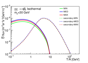
To quantify the uncertainties from the CR propagation, we consider three different propagation models, i.e. the “MIN”, “MED” and “MAX” models JIN:2014ICA . The parameters of these models are obtained by making a global fit to the AMS-02 proton flux and B/C ratio data using the GALPROP-v54  code, and the names of these models represent the typically minimal, median and maximal antiproton fluxes due to the uncertainties of propagation. The parameters of these three models are listed in Tab. 3. In our calculations, we adopt the default normalization scheme in GALPROP, which normalize the primary nuclei source term to reproduce the AMS-02 proton flux at the reference kinetic energy $T=100$ GeV.

Model	$r_{h}$(kpc)	$~{}z_{h}$(kpc)	$D_{0}$	$R_{0}$(GV)	$\delta_{1}/\delta_{2}$	$~{}V_{a}$(km/s)	$R_{ps}$(GV)	$\gamma_{p1}/\gamma_{p2}$
MIN	20	1.8	3.53	4.0	0.3/0.3	42.7	10.0	1.75/2.44
MED	20	3.2	6.50	4.0	0.29/0.29	44.8	10.0	1.79/2.45
MAX	20	6.0	10.6	4.0	0.29/0.29	43.4	10.0	1.81/2.46

TAB. 3: Values of the main parameters in the “MIN”, “MED” and “MAX” models derived from fitting to the AMS-02 $B/C$ and proton data based on the GALPROP code JIN:2014ICA . The parameter $D_{0}$ is in units of $10^{28}~{}\mathrm{cm}^{2}\cdot\mathrm{s}^{-1}$.

The $95\%$ CL upper limits of DM annihilation cross sections are derived by making a frequentist $\chi^{2}-$analysis, with $\chi^{2}$ defined as:

$$\chi^{2}=\sum_{i}\frac{(f^{\mathrm{th}}_{i}-f^{\mathrm{exp}}_{i})^{2}}{\sigma^{2}_{i}},$$ (11)

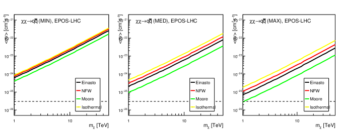
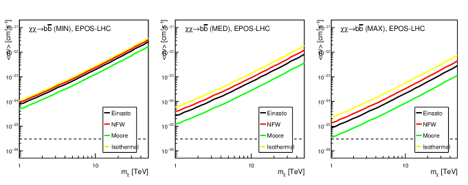
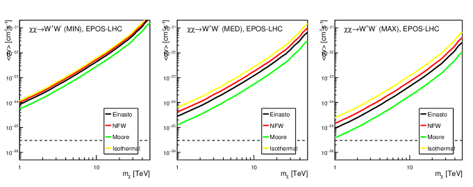
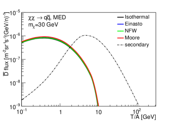
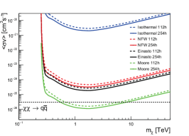
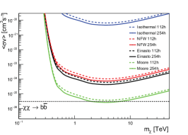
where $f^{\mathrm{exp}}_{i}$ is the central value of the experimental $\bar{p}/p$ ratio, $\sigma_{i}$ is the data error, $f^{\mathrm{exp}}_{i}$ is theoretical prediction of $\bar{p}/p$ and $i$ denotes the $i-$th data point. For the $95\%$ CL upper limits of $\bar{p}/p$ given by HAWC experiment, we set $f^{\mathrm{exp}}_{i}=0$ and the value of upper limit corresponds to $1.96\sigma_{i}$. For a specific DM mass, we first calculate the minimal value of $\chi^{2}$, and then the $95\%$ CL upper limits on DM annihilation cross sections correspond to $\Delta\chi^{2}=3.84$ for one parameter. See Ref. Jin:2015sqa for more details. The upper limits for different annihilation channels are shown in Fig. 3, with the production cross section of secondary $\bar{p}$ generated by EPOS-LHC. We can see that the differences between the upper limits for various propagation models and DM profiles can reach one to two orders of magnitude. As shown in previous works Carlson:2014ssa ; Lin:2018avl , the final flux uncertainties from propagation models and DM profiles can be larger than one order of magnitude. However, if we use these cross section upper limits to constrain the maximal flux of $\overline{\text{D}}$ and ${}^{3}\overline{\text{He}}$, the final uncertainties from the propagation model and the DM profile can be reduced to merely $30\%$ Li:2018dxj . A comparison of the maximal $\overline{\text{D}}$ fluxes in different propagation models and DM profiles are demonstrated in Fig. 4, it can be seen that the uncertainties are small.

FIG. 3: The 95$\%$ CL upper limit of DM annihilation cross sections as functions of DM particle masses, for different decay channels, propagation models and DM profiles, obtained by using the AMS-02 $\bar{p}/p$ data Aguilar:2016kjl and the HAWC $\bar{p}/p$ upper limit Abeysekara:2018syp . The energy spectrum of the secondary $\bar{p}$ are calculated by the EPOS-LHC MC generator.

FIG. 4: A comparison of the maximal $\overline{\text{D}}$ fluxes in different propagation models and DM profiles, with the DM annihilation into $q\bar{q}$ final states and DM mass $m_{\chi}=30$ GeV. The DM annihilation cross section are constrained by the AMS-02 and HAWC $\bar{p}/p$ data, with the spectrum of secondary $\bar{p}$ are calculated by using EPOS-LHC. Left) The flux results in the MED propagation model with four different DM profiles. Right) The flux results in three different propagation models, with DM profile fixed to “Isothermal”. The secondary background of the $\overline{\textrm{D}}$ flux are generated by EPOS-LHC.

IV.2 Constrains from the HESS galactic center $\gamma$-ray data

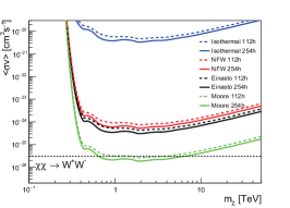
The galactic center is a promising place for detecting DM interactions, for the expected high DM density. The 10-year HESS $\gamma$-ray data Abdallah:2016ygi focus on a small area around the galactic center, and well constraints the DM annihilation cross sections for “Cuspy” type DM profiles which have large gradient at the inner galactic halo, such as the “Einasto” profile and the “NFW” profile. For DM mass $m_{\chi}\gtrsim 1$ TeV, the galactic center $\gamma$-ray can place more stringent upper limits than the $\bar{p}/p$ data. However, for “Cored” type DM profiles which are flat near the galactic center, such as the “Isothermal” profile, the constraints from the $\gamma$-ray data are relatively weak.

The latest galactic center $\gamma$-ray analysis with 254 hours exposure was published in 2016 by HESS Abdallah:2016ygi , the upper limits are calculated for several DM profiles and DM annihilation channels, but the $\gamma$-ray flux data are not released in public. Since the relative statistical error of a data point is inversely proportional to the square root of the number of counts in the bins, we can approximately estimate the 254 hours results by rescaling a previous HESS $\gamma$-ray data Abramowski:2011hc , which was published in 2011 and the exposure time are 112 hours. To obtain the upper limits for other DM profiles and channels, we perform a $\chi^{2}$ analysis to the 112 hours $\gamma$-ray flux data and estimate the 254 hours results by rescaling the data errors by a factor $\sqrt{112/254}$. The flux residual is defined as $R^{\mathrm{exp}}=F^{\mathrm{exp}}_{\mathrm{Sr}}-F^{\mathrm{exp}}_{\mathrm{Bg}}$, where $F^{\mathrm{exp}}_{\mathrm{Sr}}$ and $F^{\mathrm{exp}}_{\mathrm{Bg}}$ are experimental $\gamma$-ray flux data from the source region and from the background region respectively, and the error of $R^{\mathrm{exp}}$ is provided in Ref. Abramowski:2011hc . $R^{\mathrm{th}}=F^{\mathrm{th}}_{\mathrm{Sr}}-F^{\mathrm{th}}_{\mathrm{Bg}}$ is the theoretical value of the flux residual, and the differential flux $F^{\mathrm{th}}$ is calculated by the following formula:

$$F^{\mathrm{th}}=\frac{\mathrm{d}\Phi_{\gamma}}{\Omega\mathrm{d}E_{\gamma}}=\frac{\langle\sigma v\rangle}{8\pi m_{\chi}^{2}\Omega}\frac{\mathrm{d}N_{\gamma}}{\mathrm{d}E_{\gamma}}\int_{\Omega}\int_{\mathrm{l.o.s}}\rho^{2}(r(s,\theta))\mathrm{d}s\mathrm{d}\Omega,$$ (12)

where $\mathrm{d}N_{\gamma}/\mathrm{d}E_{\gamma}$ is the energy spectrum of photon produced in one DM annihilation, $\Omega$ is the total spherical angle of the source or background regions. We adopt the reflected background technique described in Ref. Abramowski:2011hc to determine the source region and background regions, and calculate the flux residual to make the $\chi^{2}$ analysis. We randomly choose 540 pointing positions near the GC, with the maximal distance between the pointing position and the GC is $1.5^{\circ}$. We first calculate the minimal $\chi^{2}$ value, and then the $95\%$ CL upper limit corresponds to $\Delta\chi^{2}=3.84$. The results are shown in Fig. 5. We can see that there are large gaps between the upper limits for different DM profiles. As expected, the constraints are stringent for DM profiles that are cuspy at GC, but for a cored one like “Isothermal” profile, the limits are rather weak. For various DM profiles, the constraints from $\bar{p}/p$ data are are similar, because the DM densities in the diffusion halo are similar in different DM profiles, except for the GC region. However, for $\gamma$-ray data, the GC region provides the most strigent constraints for heavy DM particles, which leads to the large gaps between DM profiles.

FIG. 5: The 95$\%$ CL upper limit of DM annihilation cross sections for different annihilation channels and DM profiles, obtained by using the HESS GC $\gamma$-ray data with 112 hours exposure Abramowski:2011hc . The 254 hours results are derived by rescaling the data errors.

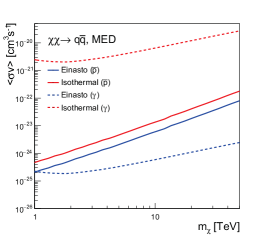
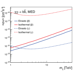
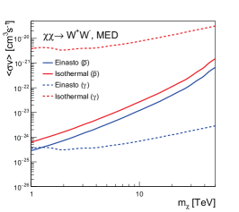
We make a comparison between the upper limits from the $\bar{p}/p$ data and from the $\gamma-$ray data, which is presented in Fig. 6. We use the “MED” propagation model as the benchmark model, and the “Isothermal” and “Einasto” profiles represent the typical “Cored” and “Cuspy” profiles respectively. The “Isothermal” profile is parameterized as follows:

$$\rho_{\mathrm{DM}}=\rho_{\odot}\frac{1+(r_{\odot}/r_{\mathrm{Iso}})^{2}}{1+(r/r_{\odot})^{2}}~{},$$ (13)

where $\rho_{\odot}=0.43~{}\mathrm{GeV/cm}^{3}$ is the local DM energy density, $r_{\mathrm{Iso}}=3.5~{}\mathrm{kpc}$. The “Einasto” profile can be written as:

$$\rho_{\mathrm{DM}}=\rho_{\odot}\exp\left[-\left(\frac{2}{\alpha}\right)\left(\frac{r^{\alpha}-r^{\alpha}_{\odot}}{r^{\alpha}_{\mathrm{Ein}}}\right)\right]~{},$$ (14)

where $\alpha=0.17$ and $r_{\mathrm{Ein}}=20$ kpc. As we can see, in all annihilation channels, for “Isothermal” profile, the upper limits from $\bar{p}/p$ data are much more stringent than the ones from $\gamma-$ray data, while for “Einasto” profile, the $\gamma-$ray data gives stricter limits than $\bar{p}/p$ for DM mass larger than 2 TeV.

It is worth mention that the Fermi-LAT experiment Atwood:2009ez also collected a large amount of $\gamma-$ray data near the GC, and the relatively large region of interest can reduce the large gaps between different DM profiles. However, the energy range of Fermi-LAT observations (from 20 MeV to more than 300 GeV) are much lower than HESS, and thus provides a weaker limitation on large DM mass. For example, the analysis in Ref. TheFermi-LAT:2017vmf show that, for a steep profile like “NFW”, HESS gives stronger constraints than Fermi-LAT at $E\gtrsim 1$ TeV. For a flat profile like “Isothermal”, the Fermi-LAT limits derived in Ref. Ackermann:2012rg are slightly weaker than the $\bar{p}/p$ constraints at $E\approx 10$ TeV. By these facts, to make the most conservative conclusion, we use the $\bar{p}/p$ limits to calculate the maximal $\overline{\text{D}}$ and ${}^{3}\overline{\text{He}}$ fluxes in “Isothermal” profile, and use the HESS $\gamma-$ray limits for “Einasto” profile in the following sections.

FIG. 6: A comparison between the upper limits from the AMS-02 and HAWC $\bar{p}/p$ data and the HESS 254 hours GC $\gamma$-ray data. The solid lines stand for constrains from the $\bar{p}/p$ data, and the dashed lines are the $\gamma$-ray limits. The “MED” propagation model are used as a benchmark model.

V The flux of $\overline{\mathrm{D}}$ and $\overline{\mathrm{He}}$ for large DM mass

V.1 DM direct annihilation

With the DM annihilation cross section upper limits at hand, we can derive the maximal $\overline{\text{D}}$ and ${}^{3}\overline{\text{He}}$ fluxes for different annihilation channels, propagation models, and DM profiles. As shown in Fig. 4, by constraining the DM annihilation cross section with the $\bar{p}/p$ data, the uncertainties from propagation models are small, thus we present our results in the “MED” propagation model, and other models do not affect our conclusions. For illustration purpose, the particle mass of the heavy DM are set to be $m_{\chi}=10$ and 50 TeV, which are smaller than the unitarity bound for a self-conjugate DM PhysRevD.100.043029 . However, it is worth mention that our analysis is largely model independent, we do not assume the DM have thermal origins.

Currently, the AMS-02 detector has the strongest detection ability for both $\overline{\text{D}}$ and ${}^{3}\overline{\text{He}}$. For $\overline{\text{D}}$ flux, the AMS-02 detection sensitivity is given in Ref. Aramaki:2015pii , while the sensitivity for ${}^{3}\overline{\text{He}}$ are only released in terms of ${}^{3}\overline{\text{He}}/\mathrm{He}$ ratio in Ref. Kounine:2010js . To study the detection prospects of AMS-02, we present our results in terms of $\overline{\text{D}}$ fluxes and ${}^{3}\overline{\text{He}}/\mathrm{He}$ ratios.

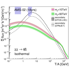
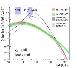
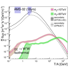
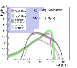
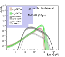
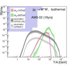
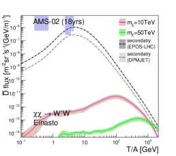
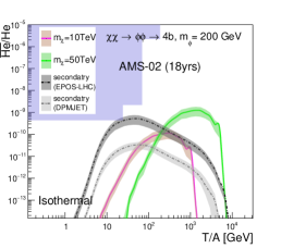
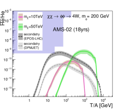
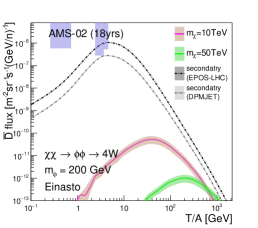
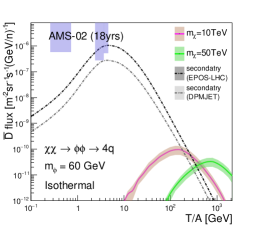
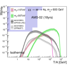
The results for “Isothermal” profile with $m_{\chi}=10$ and 50 TeV are presented in Fig. 7, with the DM annihilation cross section constrained by the AMS-02 and HAWC $\bar{p}/p$ data. The top three figures show the results about $\overline{\text{D}}$ fluxes for different annihilation channels, while the bottom three figures present the ${}^{3}\overline{\text{He}}/\mathrm{He}$ ratio results. The blue shades represent the prospective AMS-02 detection sensitivity after 18 years of data collection, and the error bands show the uncertainties from coalescence momenta. Note that for $\overline{\text{D}}$, the error bands for the secondary background are thinner than the line width. We can see that for $\overline{\text{D}}$, the DM contributions exceed the secondary backgrounds in the energy region $T/A\gtrsim 300$ GeV. For $b\bar{b}$ and $W^{+}W^{-}$ channels and $m_{\chi}=50$ TeV, the excess can be as large as one order of magnitude. Similarly, for ${}^{3}\overline{\text{He}}$, the excess exist at the kinetic energy around 800 GeV per nucleon, and the primary ${}^{3}\overline{\text{He}}$ fluxes originated by the annihilation of DM can be 20 times larger than the secondary background with $m_{\chi}=50$ TeV. Despite the fluxes of these anti-nuclei are small at high kinetic energies, and are far below the AMS-02 sensitivities, these excesses can be promising windows for future detections.

FIG. 7: The $\overline{\text{D}}$ fluxes (top figures) and the ${}^{3}\overline{\text{He}}/\mathrm{He}$ ratios (bottom figures), for the “Isothermal” profile with large DM mass and “MED” propagation model. The DM annihilation cross section is constrained by the AMS-02 and HAWC $\bar{p}/p$ data. The blue shade represents the 18-year AMS-02 detection sensitivity.

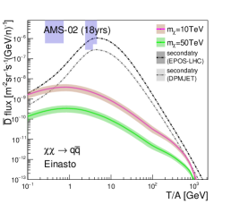
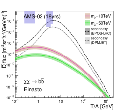
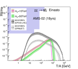
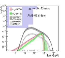
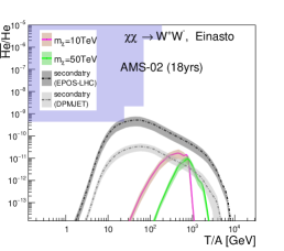
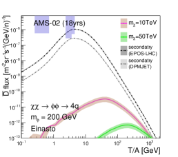
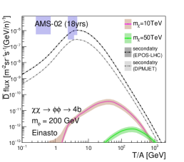
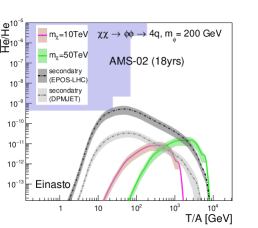
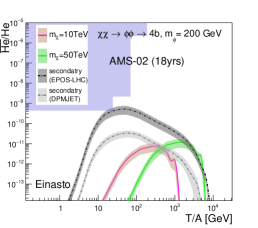
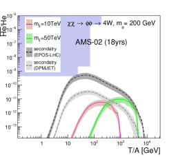
The results for “Einasto” profile are shown in Fig. 8, with the DM annihilation cross sections are constrained by the HESS 10-year GC $\gamma-$ray data. For $\overline{\text{D}}$, the DM contributions are below the secondary background in all energy regions and annihilation channels, and thus the high window closes. However, for ${}^{3}\overline{\text{He}}$, the conclusion depends on the choice of MC generators. The DM contributions are lower than the secondary background given by EPOS-LHC, but can still exceed the DPMJET-III background.

FIG. 8: The $\overline{\text{D}}$ fluxes (top figures) and the ${}^{3}\overline{\text{He}}/\mathrm{He}$ ratios (bottom figures), for the “Einasto” profile with large DM mass and “MED” propagation model. The DM annihilation cross section is constrained by the HESS 10-year GC $\gamma-$ray data. The blue shade represents the 18-year AMS-02 detection sensitivity.

V.2 DM annihilation through mediators

We also consider the process $\chi\chi\rightarrow\phi\phi\rightarrow f\bar{f}f\bar{f}$, that two DM particles first annihilate into a couple of mediators, and then the mediators decay into standard model final states. If the mass of the mediator are much smaller than the DM particle, the mediator wound be highly boosted, thus the $\overline{\text{D}}$ and ${}^{3}\overline{\text{He}}$ produced in this process are expected to assemble in high energy regions, which provides a high signal-to-background ratio for the high energy window.

By following the steps described in Sec. IV, we obtain the $95\%$ CL upper limit of cross sections for the annihilation process with mediators, the results for mediator mass $m_{\phi}=200$ GeV are presented in Fig. 9. Similar to the results for direct annihilations, for “Isothermal” profile, the most stringent constraints are from $\bar{p}/p$ data, while for “Einasto” profile, the $\gamma-$ray limitation are stricter. Again, we use the AMS-02 and HAWC $\bar{p}/p$ data to constrain the “Isothermal” profile, and the “Einasto” profile is restricted by the HESS GC $\gamma-$ray data.

FIG. 9: The 95$\%$ CL upper limit of DM annihilation cross sections for different mediator decay channels. The solid lines are derived by using the AMS-02 $\bar{p}/p$ data and the HAWC $\bar{p}/p$ upper limit, while the dashed lines represents the limits from the HESS GC $\gamma-$ray data. The energy spectrum of the secondary $\bar{p}$ are calculated by EPOS-LHC, and the “MED” propagation model are used.

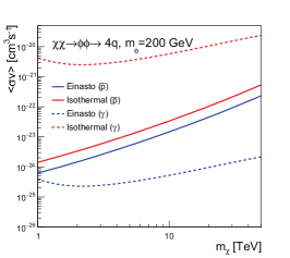
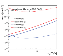
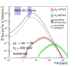
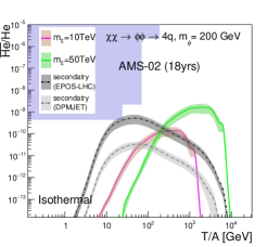
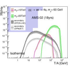
The results for “Isothermal” profile and “Einasto” profile with $m_{\phi}=200$ GeV are presented in Fig. 10 and Fig. 11 respectively. As expected, the DM contributions are boosted to high energy regions, and we get similar conclusions as in direct annihilation channels. For “Isothermal” profile with $m_{\chi}=50$ TeV, the high energy window opens for both $\overline{\text{D}}$ and ${}^{3}\overline{\text{He}}$ in all decay channels, especially for ${}^{3}\overline{\text{He}}$, the excesses can reach two order of magnitude in $q\bar{q}$ and $b\bar{b}$ channels. While for $m_{\chi}=10$ TeV, the DM contributions for $\overline{\text{D}}$ and ${}^{3}\overline{\text{He}}$ are comparable to the secondary backgrounds.

However, as shown in Fig. 11, for “Einasto” profile, the excesses in high energy regions disappear for $\overline{\text{D}}$ for all DM masses and mediator decay channels. For ${}^{3}\overline{\text{He}}$, the contributions from DM with $m_{\chi}=50$ TeV can be larger than the background calculated by using DPMJET-III. But for EPOS-LHC, the only exceed appears in $q\bar{q}$ decay channel with $m_{\chi}=50$ TeV.

FIG. 10: The $\overline{\text{D}}$ fluxes (top figures) and the ${}^{3}\overline{\text{He}}/\mathrm{He}$ ratios (bottom figures), for the “Isothermal” profile and different mediator decay channels, with the “MED” propagation model are used. The DM annihilation cross section is constrained by the AMS-02 and HAWC $\bar{p}/p$ data.

FIG. 11: The $\overline{\text{D}}$ fluxes (top figures) and the ${}^{3}\overline{\text{He}}/\mathrm{He}$ ratios (bottom figures), for the “Einasto” profile and different mediator decay channels, with the “MED” propagation model are used. The DM annihilation cross section is constrained by the HESS 10-year GC $\gamma-$ray data.

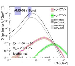
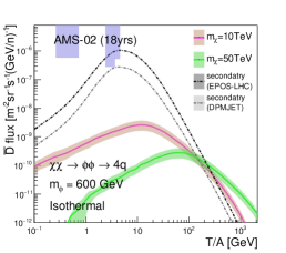
For other mediator masses, we get the same conclusion. Take the $\chi\chi\rightarrow\phi\phi\rightarrow 4q$ channel for an example, we calculate the $\overline{\text{D}}$ fluxes and ${}^{3}\overline{\text{He}}$ ratios for mediator mass $m_{\phi}=60$, 200 and 600 GeV, and present the results for “Isothermal” profile in Fig. 12. It can be seen that with the growth of the mediator mass, the DM contributions in low energy regions increase significantly. However, in high energy regions, which we are interested in, the variations of the results are small.

FIG. 12: The $\overline{\text{D}}$ fluxes (top figures) and the ${}^{3}\overline{\text{He}}/\mathrm{He}$ ratios (bottom figures), for the “Isothermal” profile and $\chi\chi\rightarrow\phi\phi\rightarrow 4q$ channels, with different mediator masses and the “MED” propagation model. The DM annihilation cross section is constrained by the AMS-02 and HAWC $\bar{p}/p$ data.

VI Conclusions

In summary, we explored the possibility of probing DM by high energy CR anti-nuclei. We used the MC generators PYTHIA 8.2, EPOS-LHC and DPMJET-III and the coalescence model to calculate the spectra of anti-nuclei, with the coalescence momenta of $\overline{\text{D}}$ and ${}^{3}\overline{\text{He}}$ were derived by fitting the data from ALICE, ALEPH and CERN ISR experiments. The propagation of charged CR particles are calculated by the GALPROP-v54 code, with the inelastic interaction cross sections between the primary CR and interstellar gases given by MC generators. We used the HESS GC $\gamma-$ray data to constrain the DM annihilation cross sections for the DM profiles with large gradient at GC, while the flat profiles were limited by the AMS-02 and HAWC $\bar{p}/p$ data.

Our results showed that, for a “Cored” type DM density profile like the “Isothermal” profile, the high energy window opened for both $\overline{\text{D}}$ and ${}^{3}\overline{\text{He}}$ in all channels. However, for a “Cuspy” type profile like the “Einasto” profile, the $\overline{\text{D}}$ contributions from DM annihilations were below the secondary background in both DM direct annihilation and annihilation through mediator decay channels. As for ${}^{3}\overline{\text{He}}$, the conclusion depended on the choice of MC generators, the ${}^{3}\overline{\text{He}}$ flux originated from DM annihilations could exceed the secondary background for DPMJET-III, while the excess disappeared for EPOS-LHC.

Signals in high energy regions can effectively avoid the uncertainties from the solar activities. Although the fluxes of $\overline{\text{D}}$ and ${}^{3}\overline{\text{He}}$ in high energy regions were far below the sensitivity of the current experiments like AMS-02 and GAPS, the high energy window could be a promising probe of DM for the next generation experiments. We believe that with the fast development of detector technologies, people would finally be able to detect the DM through the high energy window.

References

- (1) J. J. Beatty et al., “New measurement of the cosmic-ray positron fraction from 5 to 15-GeV,” Phys. Rev. Lett. 93 (2004) 241102, arXiv:astro-ph/0412230 [astro-ph].
- (2) PAMELA Collaboration, O. Adriani et al., “An anomalous positron abundance in cosmic rays with energies 1.5-100 GeV,” Nature 458 (2009) 607–609, arXiv:0810.4995 [astro-ph].
- (3) Fermi-LAT Collaboration, M. Ackermann et al., “Measurement of separate cosmic-ray electron and positron spectra with the Fermi Large Area Telescope,” Phys. Rev. Lett. 108 (2012) 011103, arXiv:1109.0521 [astro-ph.HE].
- (4) AMS Collaboration, L. Accardo et al., “High Statistics Measurement of the Positron Fraction in Primary Cosmic Rays of 0.5–500 GeV with the Alpha Magnetic Spectrometer on the International Space Station,” Phys. Rev. Lett. 113 (2014) 121101.
- (5) J. Kopp, “Constraints on dark matter annihilation from AMS-02 results,” Phys. Rev. D88 (2013) 076013, arXiv:1304.1184 [hep-ph].
- (6) L. Bergstrom, T. Bringmann, I. Cholis, D. Hooper, and C. Weniger, “New Limits on Dark Matter Annihilation from AMS Cosmic Ray Positron Data,” Phys. Rev. Lett. 111 (2013) 171101, arXiv:1306.3983 [astro-ph.HE].
- (7) A. Ibarra, A. S. Lamperstorfer, and J. Silk, “Dark matter annihilations and decays after the AMS-02 positron measurements,” Phys. Rev. D89 no. 6, (2014) 063539, arXiv:1309.2570 [hep-ph].
- (8) H.-B. Jin, Y.-L. Wu, and Y.-F. Zhou, “Implications of the first AMS-02 measurement for dark matter annihilation and decay,” JCAP 1311 (2013) 026, arXiv:1304.1997 [hep-ph].
- (9) O. Adriani et al., “Measurement of the flux of primary cosmic ray antiprotons with energies of 60-MeV to 350-GeV in the PAMELA experiment,” JETP Lett. 96 (2013) 621–627. [Pisma Zh. Eksp. Teor. Fiz.96,693(2012)].
- (10) K. Abe et al., “Measurement of the cosmic-ray antiproton spectrum at solar minimum with a long-duration balloon flight over Antarctica,” Phys. Rev. Lett. 108 (2012) 051102, arXiv:1107.6000 [astro-ph.HE].
- (11) AMS Collaboration, M. Aguilar et al., “Antiproton Flux, Antiproton-to-Proton Flux Ratio, and Properties of Elementary Particle Fluxes in Primary Cosmic Rays Measured with the Alpha Magnetic Spectrometer on the International Space Station,” Phys. Rev. Lett. 117 no. 9, (2016) 091103.
- (12) G. Giesen, M. Boudaud, Y. Génolini, V. Poulin, M. Cirelli, P. Salati, and P. D. Serpico, “AMS-02 antiprotons, at last! Secondary astrophysical component and immediate implications for Dark Matter,” JCAP 1509 no. 09, (2015) 023, arXiv:1504.04276 [astro-ph.HE].
- (13) H.-B. Jin, Y.-L. Wu, and Y.-F. Zhou, “Upper limits on dark matter annihilation cross sections from the first AMS-02 antiproton data,” Phys. Rev. D92 no. 5, (2015) 055027, arXiv:1504.04604 [hep-ph].
- (14) S.-J. Lin, X.-J. Bi, J. Feng, P.-F. Yin, and Z.-H. Yu, “Systematic study on the cosmic ray antiproton flux,” Phys. Rev. D96 no. 12, (2017) 123010, arXiv:1612.04001 [astro-ph.HE].
- (15) A. Reinert and M. W. Winkler, “A Precision Search for WIMPs with Charged Cosmic Rays,” JCAP 1801 no. 01, (2018) 055, arXiv:1712.00002 [astro-ph.HE].
- (16) F. Donato, N. Fornengo, and P. Salati, “Anti-deuterons as a signature of supersymmetric dark matter,” Phys. Rev. D62 (2000) 043003, arXiv:hep-ph/9904481 [hep-ph].
- (17) E. Carlson, A. Coogan, T. Linden, S. Profumo, A. Ibarra, and S. Wild, “Antihelium from Dark Matter,” Phys. Rev. D89 no. 7, (2014) 076005, arXiv:1401.2461 [hep-ph].
- (18) M. Cirelli, N. Fornengo, M. Taoso, and A. Vittino, “Anti-helium from Dark Matter annihilations,” JHEP 08 (2014) 009, arXiv:1401.4017 [hep-ph].
- (19) AMS Collaboration, F. Giovacchini and V. Choutko, “Cosmic Rays Antideuteron Sensitivity for AMS-02 Experiment,” in Proceedings, 30th International Cosmic Ray Conference (ICRC 2007): Merida, Yucatan, Mexico, July 3-11, 2007, vol. 4, pp. 765–768. 2007. http://indico.nucleares.unam.mx/contributionDisplay.py?contribId=1112&confId=4.
- (20) A. Kounine, “Status of the AMS Experiment,” arXiv:1009.5349 [astro-ph.HE].
- (21) GAPS Collaboration, T. Aramaki, C. J. Hailey, S. E. Boggs, P. von Doetinchem, H. Fuke, S. I. Mognet, R. A. Ong, K. Perez, and J. Zweerink, “Antideuteron Sensitivity for the GAPS Experiment,” Astropart. Phys. 74 (2016) 6–13, arXiv:1506.02513 [astro-ph.HE].
- (22) Y.-C. Ding, N. Li, C.-C. Wei, Y.-L. Wu, and Y.-F. Zhou, “Prospects of detecting dark matter through cosmic-ray antihelium with the antiproton constraints,” JCAP 1906 no. 06, (2019) 004, arXiv:1808.03612 [hep-ph].
- (23) P. von Doetinchem et al., “Cosmic-ray Antinuclei as Messengers of New Physics: Status and Outlook for the New Decade,” arXiv:2002.04163 [astro-ph.HE].
- (24) T. Sjostrand, S. Mrenna, and P. Z. Skands, “PYTHIA 6.4 Physics and Manual,” JHEP 05 (2006) 026, arXiv:hep-ph/0603175 [hep-ph].
- (25) T. Sjöstrand, S. Ask, J. R. Christiansen, R. Corke, N. Desai, P. Ilten, S. Mrenna, S. Prestel, C. O. Rasmussen, and P. Z. Skands, “An Introduction to PYTHIA 8.2,” Comput. Phys. Commun. 191 (2015) 159–177, arXiv:1410.3012 [hep-ph].
- (26) K. Werner, F.-M. Liu, and T. Pierog, “Parton ladder splitting and the rapidity dependence of transverse momentum spectra in deuteron-gold collisions at RHIC,” Phys. Rev. C74 (2006) 044902, arXiv:hep-ph/0506232 [hep-ph].
- (27) T. Pierog, I. Karpenko, J. M. Katzy, E. Yatsenko, and K. Werner, “EPOS LHC: Test of collective hadronization with data measured at the CERN Large Hadron Collider,” Phys. Rev. C92 no. 3, (2015) 034906, arXiv:1306.0121 [hep-ph].
- (28) S. Roesler, R. Engel, and J. Ranft, “The Event generator DPMJET-III at cosmic ray energies,” in 27th International Cosmic Ray Conference (ICRC 2001) Hamburg, Germany, August 7-15, 2001, pp. 439–442. 2001. http://www.copernicus.org/icrc/papers/ici6589_p.pdf.
- (29) ALEPH Collaboration, S. Schael et al., “Deuteron and anti-deuteron production in e+ e- collisions at the Z resonance,” Phys. Lett. B639 (2006) 192–201, arXiv:hep-ex/0604023 [hep-ex].
- (30) British-Scandinavian-MIT Collaboration, S. Henning et al., “Production of Deuterons and anti-Deuterons in Proton Proton Collisions at the CERN ISR,” Lett. Nuovo Cim. 21 (1978) 189.
- (31) ALICE Collaboration, S. Acharya et al., “Production of deuterons, tritons, 3He nuclei and their antinuclei in pp collisions at = 0.9, 2.76 and 7 TeV,” Phys. Rev. C97 no. 2, (2018) 024615, arXiv:1709.08522 [nucl-ex].
- (32) HAWC Collaboration, A. U. Abeysekara et al., “Constraining the ratio in TeV cosmic rays with observations of the Moon shadow by HAWC,” Phys. Rev. D97 no. 10, (2018) 102005, arXiv:1802.08913 [astro-ph.HE].
- (33) H.E.S.S. Collaboration, A. Abramowski et al., “Search for a Dark Matter annihilation signal from the Galactic Center halo with H.E.S.S,” Phys. Rev. Lett. 106 (2011) 161301, arXiv:1103.3266 [astro-ph.HE].
- (34) H.E.S.S. Collaboration, H. Abdallah et al., “Search for dark matter annihilations towards the inner Galactic halo from 10 years of observations with H.E.S.S,” Phys. Rev. Lett. 117 no. 11, (2016) 111301, arXiv:1607.08142 [astro-ph.HE].
- (35) S. T. Butler and C. A. Pearson, “Deuterons from High-Energy Proton Bombardment of Matter,” Phys. Rev. 129 (1963) 836–842.
- (36) A. Schwarzschild and C. Zupancic, “Production of Tritons, Deuterons, Nucleons, and Mesons by 30-GeV Protons on A-1, Be, and Fe Targets,” Phys. Rev. 129 (1963) 854–862.
- (37) L. P. Csernai and J. I. Kapusta, “Entropy and Cluster Production in Nuclear Collisions,” Phys. Rept. 131 (1986) 223–318.
- (38) K. Blum, K. C. Y. Ng, R. Sato, and M. Takimoto, “Cosmic rays, antihelium, and an old navy spotlight,” Phys. Rev. D96 no. 10, (2017) 103021, arXiv:1704.05431 [astro-ph.HE].
- (39) T. Aramaki et al., “Review of the theoretical and experimental status of dark matter identification with cosmic-ray antideuterons,” Phys. Rept. 618 (2016) 1–37, arXiv:1505.07785 [hep-ph].
- (40) P. Skands, S. Carrazza, and J. Rojo, “Tuning PYTHIA 8.1: the Monash 2013 Tune,” Eur. Phys. J. C74 no. 8, (2014) 3024, arXiv:1404.5630 [hep-ph].
- (41) ATLAS Collaboration, G. Aad et al., “Measurement of the transverse momentum distribution of bosons in proton–proton collisions at =7 TeV with the ATLAS detector,” Phys. Lett. B705 (2011) 415–434, arXiv:1107.2381 [hep-ex].
- (42) NA49 Collaboration, T. Anticic et al., “Inclusive production of protons, anti-protons and neutrons in p+p collisions at 158-GeV/c beam momentum,” Eur. Phys. J. C65 (2010) 9–63, arXiv:0904.2708 [hep-ex].
- (43) V. S. Berezinsky, S. V. Bulanov, V. A. Dogiel, and V. S. Ptuskin, Astrophysics of cosmic rays. 1990.
- (44) A. W. Strong, I. V. Moskalenko, and V. S. Ptuskin, “Cosmic-ray propagation and interactions in the Galaxy,” Ann. Rev. Nucl. Part. Sci. 57 (2007) 285–327, arXiv:astro-ph/0701517 [astro-ph].
- (45) A. W. Strong and I. V. Moskalenko, “Propagation of cosmic-ray nucleons in the galaxy,” Astrophys. J. 509 (1998) 212–228, arXiv:astro-ph/9807150 [astro-ph].
- (46) I. V. Moskalenko, A. W. Strong, J. F. Ormes, and M. S. Potgieter, “Secondary anti-protons and propagation of cosmic rays in the galaxy and heliosphere,” Astrophys. J. 565 (2002) 280–296, arXiv:astro-ph/0106567 [astro-ph].
- (47) A. W. Strong and I. V. Moskalenko, “Models for galactic cosmic ray propagation,” Adv. Space Res. 27 (2001) 717–726, arXiv:astro-ph/0101068 [astro-ph].
- (48) I. V. Moskalenko, A. W. Strong, S. G. Mashnik, and J. F. Ormes, “Challenging cosmic ray propagation with antiprotons. Evidence for a fresh nuclei component?,” Astrophys. J. 586 (2003) 1050–1066, arXiv:astro-ph/0210480 [astro-ph].
- (49) V. S. Ptuskin, I. V. Moskalenko, F. C. Jones, A. W. Strong, and V. N. Zirakashvili, “Dissipation of magnetohydrodynamic waves on energetic particles: impact on interstellar turbulence and cosmic ray transport,” Astrophys. J. 642 (2006) 902–916, arXiv:astro-ph/0510335 [astro-ph].
- (50) J. F. Navarro, C. S. Frenk, and S. D. M. White, “A Universal density profile from hierarchical clustering,” Astrophys. J. 490 (1997) 493–508, arXiv:astro-ph/9611107 [astro-ph].
- (51) L. Bergstrom, P. Ullio, and J. H. Buckley, “Observability of gamma-rays from dark matter neutralino annihilations in the Milky Way halo,” Astropart. Phys. 9 (1998) 137–162, arXiv:astro-ph/9712318 [astro-ph].
- (52) B. Moore, S. Ghigna, F. Governato, G. Lake, T. R. Quinn, J. Stadel, and P. Tozzi, “Dark matter substructure within galactic halos,” Astrophys. J. 524 (1999) L19–L22, arXiv:astro-ph/9907411 [astro-ph].
- (53) J. Diemand, B. Moore, and J. Stadel, “Convergence and scatter of cluster density profiles,” Mon. Not. Roy. Astron. Soc. 353 (2004) 624, arXiv:astro-ph/0402267 [astro-ph].
- (54) J. Einasto, “Dark Matter,” in Astronomy and Astrophysics 2010, [Eds. Oddbjorn Engvold, Rolf Stabell, Bozena Czerny, John Lattanzio], in Encyclopedia of Life Support Systems (EOLSS), Developed under the Auspices of the UNESCO, Eolss Publishers, Oxford ,UK. 2009. arXiv:0901.0632 [astro-ph.CO]. http://inspirehep.net/record/810367/files/arXiv:0901.0632.pdf.
- (55) M. Korsmeier, F. Donato, and N. Fornengo, “Prospects to verify a possible dark matter hint in cosmic antiprotons with antideuterons and antihelium,” Phys. Rev. D97 no. 10, (2018) 103011, arXiv:1711.08465 [astro-ph.HE].
- (56) L. J. Gleeson and W. I. Axford, “Solar Modulation of Galactic Cosmic Rays,” Astrophys. J. 154 (1968) 1011.
- (57) H.-B. Jin, Y.-L. Wu, and Y.-F. Zhou, “Cosmic ray propagation and dark matter in light of the latest AMS-02 data,” JCAP 1509 no. 09, (2015) 049, arXiv:1410.0171 [hep-ph].
- (58) S.-J. Lin, X.-J. Bi, and P.-F. Yin, “Expectations of the Cosmic Antideuteron Flux,” arXiv:1801.00997 [astro-ph.HE].
- (59) Fermi-LAT Collaboration, W. B. Atwood et al., “The Large Area Telescope on the Fermi Gamma-ray Space Telescope Mission,” Astrophys. J. 697 (2009) 1071–1102, arXiv:0902.1089 [astro-ph.IM].
- (60) Fermi-LAT Collaboration, M. Ackermann et al., “The Fermi Galactic Center GeV Excess and Implications for Dark Matter,” Astrophys. J. 840 no. 1, (2017) 43, arXiv:1704.03910 [astro-ph.HE].
- (61) Fermi-LAT Collaboration, M. Ackermann et al., “Constraints on the Galactic Halo Dark Matter from Fermi-LAT Diffuse Measurements,” Astrophys. J. 761 (2012) 91, arXiv:1205.6474 [astro-ph.CO].
- (62) J. Smirnov and J. F. Beacom, “Tev-scale thermal wimps: Unitarity and its consequences,” Phys. Rev. D 100 (Aug, 2019) 043029. https://link.aps.org/doi/10.1103/PhysRevD.100.043029.