Bidirectional compression in heterogeneous settings for distributed or federated learning with partial participation: tight convergence guarantees

Abstract

We introduce a framework – Artemis – to tackle the problem of learning in a distributed or federated setting with communication constraints and device partial participation. Several workers (randomly sampled) perform the optimization process using a central server to aggregate their computations. To alleviate the communication cost, Artemis allows to compress the information sent in both directions (from the workers to the server and conversely) combined with a memory mechanism. It improves on existing algorithms that only consider unidirectional compression (to the server), or use very strong assumptions on the compression operator, and often do not take into account devices partial participation. We provide fast rates of convergence (linear up to a threshold) under weak assumptions on the stochastic gradients (noise’s variance bounded only at optimal point) in non-i.i.d. setting, highlight the impact of memory for unidirectional and bidirectional compression, analyze Polyak-Ruppert averaging. We use convergence in distribution to obtain a lower bound of the asymptotic variance that highlights practical limits of compression. We propose two approaches to tackle the challenging case of devices partial participation and provide experimental results to demonstrate the validity of our analysis.

1 Introduction

In modern large scale machine learning applications, optimization has to be processed in a distributed fashion, using a potentially large number $N$ of workers. In the data-parallel framework, each worker only accesses a fraction of the data: new challenges have arisen, especially when communication constraints between the workers are present.

In this paper, we focus on first-order methods, especially Stochastic Gradient Descent [Bottou, 1999; Robbins & Monro, 1951] in a centralized framework: a central machine aggregates the computation of the $N$ workers in a synchronized way. This applies to both the distributed [e.g. Li et al., 2014] and the federated learning [introduced in Konečný et al., 2016; McMahan et al., 2017] settings.

Formally, we consider a number of features $d\in\mathbb{N^{*}}$, and a convex cost function $F:\mathbb{R}^{d}\rightarrow\mathbb{R}$. We want to solve the following convex optimization problem:

$$\min_{w\in\mathbb{R}^{d}}F(w)\text{ with }F(w)=\frac{1}{N}\sum_{i=1}^{N}F_{i}(w)\,,\vspace{-.5em}$$ (1)

where $(F_{i})_{i=1}^{N}$ is a local risk function for the model $w$ on the worker $i$. Especially, in the classical supervised machine learning framework, we fix a loss $\ell$ and access, on a worker $i$, $n_{i}$ observations $(z^{i}_{k})_{1\leq k\leq n_{i}}$ following a distribution $D_{i}$. In this framework, $F_{i}$ can be either the (weighted) local empirical risk, $w\mapsto(n_{i}^{-1})\sum_{k=1}^{n_{i}}\ell(w,z^{i}_{k})$ or the expected risk $w\mapsto\mathbb{E}_{z\sim D_{i}}[\ell(w,z)]$. At each iteration of the algorithm, each worker can get an unbiased oracle on the gradient of the function $F_{i}$ (typically either by choosing uniformly an observation in its dataset or in a streaming fashion, getting a new observation at each step).

Our goal is to reduce the amount of information exchanged between workers, to accelerate the learning process, limit the bandwidth usage, and reduce energy consumption. Indeed, the communication cost has been identified as an important bottleneck in the distributed settings [e.g. Strom, 2015]. In their overview of the federated learning framework, Kairouz et al. [2019] also underline in Section 3.5 two possible directions to reduce this cost: 1) compressing communication from workers to the central server (uplink) 2) compressing the downlink communication.

Most of the papers considering the problem of reducing the communication cost [Alistarh et al., 2017; Agarwal et al., 2018; Wu et al., 2018; Karimireddy et al., 2019; Mishchenko et al., 2019; Horváth et al., 2019; Li et al., 2020; Horváth & Richtárik, 2020] only focus on compressing the message sent from the workers to the central node. This direction has the highest potential to reduce the total runtime given that (i) the bandwidth for upload is generally more limited than for download, and that (ii) for some regimes with a large number of workers, the downlink communication, that corresponds to a “one-to-$N$” communication, may not be the bottleneck compared to the “$N$-to-one” uplink.

Nevertheless, there are several reasons to also consider downlink compression. First, the difference between upload and download speeds is not significant enough at all to ignore the impact of the downlink direction (see Appendix B for an analysis of bandwidth). If we consider for instance a small number $N$ of workers training a very heavy model – the size of Deep Learning models generally exceeds hundreds of MB [Dean et al., 2012; Huang et al., 2019] –, the training speed will be limited by the exchange time of the updates, thus using downlink compression is key to accelerating the process. Secondly, in a different framework in which a network of smartphones collaborate to train a large scale model in a federated framework, participants to the training would not be eager to download a hundreds of MB for each update on their phone. Here again, downlink compression appears to be necessary. To encompass all situations, our framework implements compression in either or both directions with possibly different compression levels.

Bidirectional compression (i.e. compressing both uplink and downlink) raises new challenges. In the downlink step, if we compress the model, the quantity compressed does not tend to zero. Consequently the compression error significantly hinders convergence. To circumvent this problem we compress the gradient that may asymptotically approach zero. Double compression has been recently considered by Tang et al. [2019]; Zheng et al. [2019]; Liu et al. [2020]; Yu et al. [2019]; Philippenko & Dieuleveut [2021]. One of the most recent work, Dore, defined by Liu et al. [2020], analyzed a double compression approach, combining error compensation, a memory mechanism and model compression, with a uniform bound on the gradient variance. In this work, we provide new results on Dore-like algorithms, considering a framework without error-feedback using tighter assumptions, and quantifying precisely the impact of data heterogeneity on the convergence.

Moreover, we focus on a heterogeneous setting: the data distribution depends on each worker (thus non i.i.d.). We explicitly control the differences between distributions. In such a setting, the local gradient at the optimal point $\nabla F_{i}(w_{*})$ may not vanish: to get a vanishing compression error, we introduce a “memory” process [Mishchenko et al., 2019]. A very recent work by Philippenko & Dieuleveut [2021] builds upon our demonstrations precisely to handle non-i.i.d. settings; however they introduce an additional mechanism (“preserved update”) that is orthogonal to this work.

Finally, we encompass in Artemis Partial Participation (PP) settings, in which only some workers contribute to each step. Several challenges arise with PP, because of both heterogeneity and downlink compression. We propose a new algorithm in that setting, which improves on the approaches proposed by Sattler et al. [2019]; Tang et al. [2019] for bidirectional compression.

Assumptions made on the gradient oracle directly influence the convergence rate of the algorithm: in this paper, we neither assume that the gradients are uniformly bounded [as in Zheng et al., 2019] nor that their variance is uniformly bounded [as in Alistarh et al., 2017; Mishchenko et al., 2019; Liu et al., 2020; Tang et al., 2019; Horváth et al., 2019]: instead we only assume that the variance is bounded by a constant $\sigma_{*}^{2}$ at the optimal point $w_{*}$, and provide linear convergence rates up to a threshold proportional to $\sigma_{*}^{2}$ (as in [Dieuleveut et al., 2018; Gower et al., 2019] for non distributed optimization). This is a fundamental difference as the variance bound at the optimal point can be orders of magnitude smaller than the uniform bound used in previous work: this is striking when all loss functions have the same critical point, and thus the noise at the optimal point is null! This happens for example in the interpolation regime, which has recently gained importance in the machine learning community [Belkin et al., 2019]. As the empirical risk at the optimal point is null or very close to zero, so are all the loss functions with respect to one example. This is often the case in deep learning [e.g., Zhang et al., 2017] or in large dimension regression [Mei & Montanari, 2019].

Overall, we make the following contributions:

1. We describe a framework – Artemis – that encompasses $6$ algorithms (with or without up/down compression, with or without memory) which is adapted to PP. We provide and analyze in Theorem 1 a fast rate of convergence – exponential convergence up to a threshold proportional to $\sigma_{*}^{2}$, the noise at the optimal point –, obtaining tighter bounds than in [Alistarh et al., 2017; Mishchenko et al., 2019].

2. We explicitly tackle heterogeneity using Assumption 4, proving that the limit variance of Artemis with memory is independent from the difference between distributions (as for SGD). This is the first theoretical guarantee for double compression that explicitly quantifies the impact of non i.i.d. data.

3. We propose two approaches to tackle the case of partial device participation when using memories. This setting is challenging due to the difficulty to synchronize memories. The second (and recommended) approach leverages the full potential of the memory to improve convergence.

4. In the non strongly-convex case, we prove the convergence using Polyak-Ruppert averaging in Theorem 2.

5. We prove convergence in distribution of the iterates, and subsequently provide a lower bounds on the asymptotic variance. This sheds light on the limits of (double) compression, which results in an increase of the algorithm’s variance, and can thus only accelerate the learning process for early iterations and up to a “moderate” accuracy. Interestingly, this “moderate” accuracy has to be understood with respect to the reduced noise $\sigma_{*}^{2}$.

Furthermore, we support our analysis with various experiments illustrating the behavior of our new algorithm and we provide the code to reproduce our experiments. See this anonymized repository. In Table 1, we highlight the main features and assumptions of Artemis compared to recent algorithms using compression.

Table 1: Comparison of frameworks for main algorithms handling (bidirectional) compression. By “non i.i.d.”, we mean that the theoretical framework encompasses and explicitly quantifies the impact of data heterogeneity on convergence (Assumption 4), e.g., Dore does not assume i.i.d. workers but does not quantify differences between distributions. References: see Alistarh et al. [2017] for QSGD, Mishchenko et al. [2019] for Diana, Horváth & Richtárik [2020] for [HR20], Liu et al. [2020] for Dore, Philippenko & Dieuleveut [2021] for MCM and Tang et al. [2019] for DoubleSquezze

. QSGD Diana [HR20] Dore Double Squeeze Dist EF-SGD MCM Artemis (new) Data i.i.d. non i.i.d. non i.i.d. i.i.d. i.i.d. i.i.d. non i.i.d. non i.i.d. Bounded variance Uniformly Uniformly Uniformly Uniformly Uniformly Uniformly Uniformly At optimal point Compression One-way One-way One-way Two-way Two-way Two-way Two-way Two-way Error-feedback ✓ ✓ ✓ ✓ Memory ✓ ✓ ✓ ✓ Device sampling ✓ ✓ ✓

The rest of the paper is organized as follows: in Section 2 we introduce the framework of Artemis. In Subsection 2.1 we describe the assumptions, and we review related work in Subsection 2.2. We then give the theoretical results in Section 3, we extend the result to device sampling in Section 4, we present experiments in Section 5, and finally, we conclude in Section 6.

2 Problem statement

We consider the problem described in Equation 1. In the convex case, we assume that there exist at least one optimal point which we denote $w_{*}$, we also denote $h_{*}^{i}=\nabla F_{i}(w_{*})$, for $i$ in $\llbracket 1,N\rrbracket$. We use $\left\|\cdot\right\|$ to denote the Euclidean norm. To solve this problem, we rely on a stochastic gradient descent (SGD) algorithm.

A stochastic gradient $\textsl{g}_{k+1}^{i}$ is provided at iteration $k$ in $\mathbb{N}$ to the device $i$ in $\llbracket 1,N\rrbracket$. This function is then evaluated at point $w_{k}$: to alleviate notation, we will use $g_{k+1}^{i}=\textsl{g}_{k+1}^{i}(w_{k})$ and $g_{k+1,*}^{i}=\textsl{g}_{k+1}^{i}(w_{*})$ to denote the stochastic gradient vectors at points $w_{k}$ and $w_{*}$ on device $i$. In the classical centralized framework (without compression), with partial participation of devices, SGD corresponds to:

$$w_{k+1}=w_{k}-\gamma\frac{1}{N}\sum_{i=1}^{N}g_{k+1}^{i}\vspace{-.5em}\vspace{-.5em}\vspace{-.5em}$$ (2)

where $\gamma$ is the learning rate. Here, we first consider the full participation case.

However, computing such a sequence would require the nodes to send either the gradient $g_{k+1}^{i}$ or the updated local model to the central server (uplink communication), and the central server to broadcast back either the averaged gradient $g_{k+1}$ or the updated global model (downlink communication). Here, in order to reduce communication cost, we perform a bidirectional compression. More precisely, we combine two main tools: 1) an unbiased compression operator $\mathcal{C}:\mathbb{R}^{d}\rightarrow\mathbb{R}^{d}$ that reduces the number of bits exchanged, and 2) a memory process that reduces the size of the signal to compress, and consequently the error [Mishchenko et al., 2019; Li et al., 2020]. That is, instead of directly compressing the gradient, we first approximate it by the memory term and, afterwards, we compress the difference. As a consequence, the compressed term tends in expectation to zero, and the error of compression is reduced. Following Tang et al. [2019], we always broadcast gradients and never models. To distinguish the two compression operations we denote $\mathcal{C}_{\mathrm{up}}$ and $\mathcal{C}_{\mathrm{dwn}}$ the compression operator for downlink and uplink. At each iteration, we thus have the following steps:

1. First, each active local node sends to the central server a compression of gradient differences: $\widehat{\Delta}_{k}^{i}=\mathcal{C}_{\mathrm{up}}(g_{k+1}^{i}-h_{k}^{i})$, and updates the memory term $h_{k+1}^{i}=h^{i}_{k}+\alpha\widehat{\Delta}_{k}^{i}$ with $\alpha\in\mathbb{R}^{*}$. The server recovers the approximated gradients’ values by adding the received term to the memories kept on its side.

2. Then, the central server sends back the compression of the sum of compressed gradients: $\Omega_{k+1}=\mathcal{C}_{\mathrm{dwn}}\left(\frac{\displaystyle 1}{\displaystyle N}\sum_{i=1}^{N}\widehat{\Delta}_{k}^{i}+h_{k}^{i}\right)$. No memory mechanism needs to be used, as the sum of gradients tends to zero in the absence of regularization.

The update is thus given by:

$$\left\{\begin{array}[]{l}\forall i\in\llbracket 1,N\rrbracket\,,\quad\widehat{\Delta}_{k}^{i}=\mathcal{C}_{\mathrm{up}}\left(g_{k+1}^{i}-h_{k}^{i}\right)\\ \Omega_{k+1}=\mathcal{C}_{\mathrm{dwn}}\left(\frac{\displaystyle 1}{\displaystyle N}\sum_{i=1}^{N}(\widehat{\Delta}_{k}^{i}+h_{k}^{i})\right)\\ w_{k+1}=w_{k}-\gamma\Omega_{k+1}\end{array}\right..$$ (6)

Constants $\gamma,\alpha\in\mathbb{R}^{*}\times\mathbb{R}_{+}$ are learning rates for respectively the iterate sequence and the memory sequence. The adaptation of the framework in the case of device sampling is developed in Section 4. This is illustrated on Algoalgorithms 1 and S1 in Appendix A.

As a summary, the Artemis framework encompasses in particular these four algorithms: the variant with unidirectional compression ($\omega_{\mathcal{C}}^{\mathrm{dwn}}=0$) w.o. or with memory ($\alpha=0$ or $\alpha\neq 0$) recovers QSGD defined by Alistarh et al. [2017] and DIANA proposed by Mishchenko et al. [2019]. The variant using bidirectional compression ($\omega_{\mathcal{C}}^{\mathrm{dwn}}\neq 0$) w.o memory ($\alpha=0$) is called Bi-QSGD. The last and most effective variant combines bidirectional compression with memory and is the one we refer to as Artemis if no precision is given. It corresponds to a simplified version of Dore without error-feedback, but this additional mechanism did not lead to any theoretical improvement [Remark 2 in Sec. 4.1., Liu et al., 2020].

Remark 1 (Local steps).

An obvious independent direction to reduce communication is to increase the number of steps performed before communication. This is the spirit of Local-SGD [Stich, 2019]. It is an interesting extension to incorporate this into our framework, that we do not consider in order to focus on the compression insights.

In the following section, we present and discuss assumptions over the function $F$, the data distribution and the compression operator.

2.1 Assumptions

We make classical assumptions on $F:\mathbb{R}^{d}\rightarrow\mathbb{R}$.

Assumption 1 (Strong convexity).

$F$ is $\mu$-strongly convex, that is for all vectors $w,v$ in $\mathbb{R}^{d}$: $F(v)\geq F(w)+(v-w)^{T}\nabla F(w)+\frac{\mu}{2}\|v-w\|^{2}_{2}\,.$

Note that we do not need each $F_{i}$ to be strongly convex, but only $F$. Also remark that we only use this inequality for $v=w_{*}$ in the proof of Theorems 1 and 2.

Below, we introduce cocoercivity [see Zhu & Marcotte, 1996, for more details about this hypothesis]. This assumption implies that all $(F_{i})_{i\in\llbracket 1,N\rrbracket}$ are $L$-smooth.

Assumption 2 (Cocoercivity of stochastic gradients (in quadratic mean)).

We suppose that for all $k$ in $\mathbb{N}$, stochastic gradients functions $(\textsl{g}_{k}^{i})_{i\in\llbracket 1,N\rrbracket}$ are L-cocoercive in quadratic mean. That is, for $k$ in $\mathbb{N}$, $i$ in $\llbracket 1,N\rrbracket$ and for all vectors $w_{1},w_{2}$ in $\mathbb{R}^{d}$, we have:$\mathbb{E}[\|\textsl{g}^{i}_{k}(w_{1})-\textsl{g}_{k}^{i}(w_{2})\|^{2}]\leq L\left\langle\nabla F_{i}(w_{1})-\nabla F_{i}(w_{2})\leavevmode\nobreak\ \middle|\leavevmode\nobreak\ w_{1}-w_{2}\right\rangle\,.$

E.g., this is true under the much stronger assumption that stochastic gradients functions $(\textsl{g}_{k}^{i})_{i\in\llbracket 1,N\rrbracket}$ are almost surely $L$-cocoercive, i.e.: $\|\textsl{g}^{i}_{k}(w_{1})-\textsl{g}_{k}^{i}(w_{2})\|^{2}\leq L\left\langle\textsl{g}^{i}_{k}(w_{1})-\textsl{g}_{k}^{i}(w_{2})\leavevmode\nobreak\ \middle|\leavevmode\nobreak\ w_{1}-w_{2}\right\rangle\,$. Next, we present the assumption on the stochastic gradient’s noise. Again, we highlight that the noise is only controlled at the optimal point. To carefully control the noises process (gradient oracle, uplink and downlink compression), we introduce three filtrations $(\mathcal{H}_{k},\mathcal{G}_{k},\mathcal{F}_{k})_{k\geq 0}$, such that $w_{k}$ is $\mathcal{H}_{k}$-measurable for any $k\in\mathbb{N}$. Detailed definitions are given in Subsection A.3.

Assumption 3 (Noise over stochastic gradients computation).

The noise over stochastic gradients at the global optimal point, for a mini-batch of size $b$, is bounded: there exists a constant $\sigma_{*}\in\mathbb{R}$, s. t. for all $k$ in $\mathbb{N}$, for all $i$ in $\llbracket 1,N\rrbracket\,$, we have a.s.: $\quad\mathbb{E}[\|g_{k+1,*}^{i}-\nabla F_{i}(w_{*})\|^{2}|\mathcal{H}_{k}]\leq\frac{\sigma_{*}^{2}}{b}.$

The constant $\sigma_{*}^{2}$ is null, e.g. if we use deterministic (batch) gradients, or in the interpolation regime for i.i.d. observations, as discussed in the Introduction. As we have also incorporated here a mini-batch parameter, this reduces the variance by a factor $b$.

Unlike Diana [Mishchenko et al., 2019; Li et al., 2020], Dore [Liu et al., 2020], Dist-EF-SGD [Zheng et al., 2019], MCM [Philippenko & Dieuleveut, 2021] or Double-Squeeze [Tang et al., 2019], we assume that the variance of the noise is bounded only at optimal point $w_{*}$ and not at any point $w$ in $\mathbb{R}^{d}$. It results that if variance is null ($\sigma_{*}^{2}=0$) at optimal point, we obtain a linear convergence while previous results obtain this rate solely if the variance is null at any point (i.e. only for deterministic GD). Also remark that Assumptions 2 and 3 both stand for the simplest Least-Square Regression (LSR) setting, while the uniform bound on the gradient’s variance does not. Next, we give the assumption that links the distributions on the different machines.

Assumption 4 (Bounded gradient at $w_{*}$).

There exists a constant $B\in\mathbb{R_{+}}$, s.t.: $\frac{1}{N}\sum_{i=0}^{N}\|\nabla F_{i}(w_{*})\|^{2}=B^{2}\,.$

This assumption is used to quantify how different the distributions are on the different machines. In the streaming i.i.d. setting – $D_{1}=\dots=D_{N}$ and $F_{1}=\dots=F_{N}$ – the assumption is satisfied with $B=0$. Combining Assumptions 3 and 4 results in an upper bound on the averaged squared norm of stochastic gradients at $w_{*}$: for all $k$ in $\mathbb{N}$, a.s., $\frac{1}{N}\sum_{i=1}^{N}\mathbb{E}[\|g_{k+1,*}^{i}\|^{2}|\mathcal{H}_{k}]\leq\frac{\displaystyle\sigma_{*}^{2}}{\displaystyle b}+B^{2}$.

Finally, compression operators can be classified in two main categories: quantization [as in Alistarh et al., 2017; Seide et al., 2014; Zhou et al., 2018; Wen et al., 2017; Reisizadeh et al., 2020; Horváth et al., 2019] and sparsification [as in Stich et al., 2018; Aji & Heafield, 2017; Alistarh et al., 2018; Khirirat et al., 2020]. Theoretical guarantees provided in this paper do not rely on a particular kind of compression, as we only consider the following assumption on the compression operators $\mathcal{C}_{\mathrm{up}}$ and $\mathcal{C}_{\mathrm{dwn}}$:

Assumption 5.

There exist constants $\omega_{\mathcal{C}}^{\mathrm{up}}\,,\omega_{\mathcal{C}}^{\mathrm{dwn}}\in\mathbb{R}^{*}_{+}$, such that the compression operators $\mathcal{C}_{\mathrm{up}}$ and $\mathcal{C}_{\mathrm{dwn}}$ verify the two following properties for all $\Delta$ in $\mathbb{R}^{d}$:

$$\left\{\begin{array}[]{ll}\mathbb{E}[\mathcal{C}_{\mathrm{up}/\mathrm{dwn}}(\Delta)]=\Delta\,,\\ \mathbb{E}[\left\|\mathcal{C}_{\mathrm{up}/\mathrm{dwn}}(\Delta)-\Delta\right\|^{2}]\leq\omega_{\mathcal{C}}^{\mathrm{up}/\mathrm{dwn}}\left\|\Delta\right\|^{2}\,.\end{array}\right.$$

In other words, the compression operators are unbiased and their variances are bounded. Note that Horváth & Richtárik [2020] have shown that using an unbiased operator leads to better performances. Unlike us, Tang et al. [2019] assume uniformly bounded compression error, which is a much more restrictive assumption. We now provide additional details on related papers dealing with compression. Also note that $\omega_{\mathcal{C}}^{\mathrm{up}/\mathrm{dwn}}$ can be considered as parameters of the algorithm, as the compression levels can be chosen.

2.2 Related work on compression

Quantization is a common method for compression and is used in various algorithms. For instance, Seide et al. [2014] are one of the first to propose to quantize each gradient component by either $-1$ or $1$. This approach has been extended in Karimireddy et al. [2019]. Alistarh et al. [2017] define a new algorithm – QSGD – which instead of sending gradients, broadcasts their quantized version, getting robust results with this approach. On top of gradient compression, Wu et al. [2018] add an error compensation mechanism which accumulates quantization errors and corrects the gradient computation at each iteration. Diana [introduced in Mishchenko et al., 2019] introduces a “memory” term in the place of accumulating errors. Li et al. [2020] extend this algorithm and improve its convergence by using an accelerated gradient descent. Reisizadeh et al. [2020] combine unidirectional quantization with device sampling, leading to a framework closer to Federated Learning settings where devices can easily be switched off. In the same perspective, Horváth & Richtárik [2020] detail results that also consider PP. Tang et al. [2019] are the the first to suggest a bidirectional compression scheme for a decentralized network. For both uplink and downlink, the method consists in sending a compression of gradients combined with an error compensation. Later, Yu et al. [2019] choose to compress models instead of compressing gradients. This approach is enhanced by Liu et al. [2020] who combine model compression with a memory mechanism and an error compensation drawing from Mishchenko et al. [2019]. Both Tang et al. [2019] and Zheng et al. [2019] compress gradients without using a memory mechanism. However, as proved in the following section, memory is key to reducing the asymptotic variance in the heterogeneous case. A recent work written by Philippenko & Dieuleveut [2021] build upon our work and design an algorithm that is doing bidirectional compression but achieves rates of convergence identical to unidirectional compression. In their work, they take advantage of the uplink memory to handle the heterogeneous settings by reusing our demonstration’s paradigm.

We now provide theoretical results about the convergence of bidirectional compression.

3 Theoretical results

In this section, we present our main theoretical results on the convergence of Artemis and its variants. For the sake of clarity, the most complete and tightest versions of theorems are given in Appendices, and simplified versions are provided here. The main linear convergence rates are given in Theorem 1. In Theorem 2 we show that Artemis combined with Polyak-Ruppert averaging reaches a sub-linear convergence rate. In this section, we denote $\delta_{0}^{2}=\left\|w_{0}-w_{*}\right\|^{2}$.

Theorem 1 (Convergence of Artemis).

Under Assumptions 1, 2, 3, 4 and 5, for a step size $\gamma$ satisfying the conditions in Table 3, for a learning rate $\alpha$ and for any $k$ in $\mathbb{N}$, the mean squared distance to $w_{*}$ decreases at a linear rate up to a constant of the order of $E$:

$$\mathbb{E}\left[\left\|w_{k}-w_{*}\right\|^{2}\right] \leq(1-\gamma\mu)^{k}\left(\delta_{0}^{2}+2C\gamma^{2}B^{2}\right)+\frac{2\gamma E}{\mu N}\,,$$

for constants $C$ and $E$ depending on the variant (independent of $k$) given in Table 2 or in the appendix. Variants with $\alpha\neq 0$ require $\alpha\in[1/2(\omega_{\mathcal{C}}^{\mathrm{up}}+1),\alpha_{\max}]$, the upper bound $\alpha_{\max}$ is given in Theorem S6.

Table 2: Details on constants $C$ and $E$ defined in Theorem 1. $C=0$ for $\alpha=0$, see Th. S6 for $\alpha\neq 0$.

$\alpha$	$E$
$0$	$(\omega_{\mathcal{C}}^{\mathrm{dwn}}+1)\left((\omega_{\mathcal{C}}^{\mathrm{up}}+1)\frac{\displaystyle\sigma_{*}^{2}}{\displaystyle b}+\omega_{\mathcal{C}}^{\mathrm{up}}B^{2}\right)$
$\neq 0$	$\frac{\displaystyle\sigma_{*}^{2}}{\displaystyle b}\left((2\omega_{\mathcal{C}}^{\mathrm{up}}+1)(\omega_{\mathcal{C}}^{\mathrm{dwn}}+1)+4\alpha^{2}C(\omega_{\mathcal{C}}^{\mathrm{up}}+1)-2\alpha C\right)$

This theorem is derived from Theorems S5 and S6 which are respectively proved in Subsections E.1 and E.2. We can make the following remarks:

1. Linear convergence. The convergence rate given in Theorem 1 can be decomposed into two terms: a bias term, forgotten at linear speed $(1-\gamma\mu)^{k}$, and a variance residual term which corresponds to the saturation level of the algorithm. The rate of convergence $(1-\gamma\mu)$ does not depend on the variant of the algorithm. However, the variance and initial bias do vary.

2. Bias term. The initial bias always depends on $\left\|w_{0}-w_{*}\right\|^{2}$, and when using memory (i.e. $\alpha\neq 0$) it also depends on the difference between distributions (constant $B^{2}$).

3. Variance term and memory. On the other hand, the variance depends a) on both $\sigma_{*}^{2}/b$, and the distributions’ difference $B^{2}$ without memory b) only on the gradients’ variance at the optimum $\sigma_{*}^{2}/b$ with memory. Similar theorems in related literature Liu et al. [2020]; Alistarh et al. [2017]; Mishchenko et al. [2019]; Yu et al. [2019]; Tang et al. [2019]; Zheng et al. [2019] systematically had a worse bound for the variance term depending on a uniform bound of the noise variance or under much stronger conditions on the compression operator. This paper and [Liu et al., 2020] are also the first to give a linear convergence up to a threshold for bidirectional compression.

4. Impact of memory. To the best of our knowledge, this is the first work on double compression that explicitly tackles the non i.i.d. case (Philippenko & Dieuleveut [2021] also handle this setting but have mentioned that they get inspired from our work). We prove that memory makes the saturation threshold independent of $B^{2}$ for Artemis.

5. Variance term. The variance term increases with a factor proportional to $\omega_{\mathcal{C}}^{\mathrm{up}}$ for the unidirectional compression, and proportional to $\omega_{\mathcal{C}}^{\mathrm{up}}\times\omega_{\mathcal{C}}^{\mathrm{dwn}}$ for bidirectional. This is the counterpart of compression, each compression resulting in a multiplicative factor on the noise. A similar increase in the variance appears in [Mishchenko et al., 2019] and [Liu et al., 2020]. The noise level is attenuated by the number of devices $N$, to which it is inversely proportional.

6. Link with classical SGD. For variant of Artemis with $\alpha=0$, if $\omega_{\mathcal{C}}^{\mathrm{up}/\mathrm{dwn}}=0$ (i.e. no compression) we recover SGD results: convergence does not depend on $B^{2}$, but only on the noise’s variance.

Conclusion: Overall, it appears that Artemis is able to efficiently accelerate the learning during first iterations, enjoying the same linear rate as SGD with lower communication complexity, but it saturates at a higher level, proportional to $\sigma_{*}^{2}$ and independent of $B^{2}$.

The range of acceptable learning rates is an important feature for first order algorithms. In Table 3, we summarize the upper bound $\gamma_{\max}$ on $\gamma$, to guarantee a $(1-\gamma\mu)$ convergence of Artemis. These bounds are derived from Theorems S5 and S6, in three main asymptotic regimes: $N\gg\omega_{\mathcal{C}}^{\mathrm{up}}$, $N\approx\omega_{\mathcal{C}}^{\mathrm{up}}$ and $\omega_{\mathcal{C}}^{\mathrm{up}}\gg N$. Using bidirectional compression impacts $\gamma_{\max}$ by a factor $\omega_{\mathcal{C}}^{\mathrm{dwn}}+1$ in comparison to unidirectional compression. For unidirectional compression, if the number of machines is at least of the order of $\omega_{\mathcal{C}}^{\mathrm{up}}$, then $\gamma_{\max}$ nearly corresponds to $\gamma_{\max}$ for vanilla (serial) SGD.

Table 3: Upper bound on $\gamma_{\max}$ to guarantee convergence. For unidirectional compression (resp. no compr.), $\omega_{\mathcal{C}}^{\mathrm{dwn}}=0$ (resp. $\omega_{\mathcal{C}}^{\mathrm{up}/\mathrm{dwn}}=0$, recovering classical rates for SGD).

Memory	$\alpha=0$	$\alpha\neq 0$
$N\gg\omega_{\mathcal{C}}^{\mathrm{up}}$	$\frac{\displaystyle 1}{\displaystyle(\omega_{\mathcal{C}}^{\mathrm{dwn}}+1)L}$	$\frac{\displaystyle 1}{\displaystyle 2(\omega_{\mathcal{C}}^{\mathrm{dwn}}+1)L}$
$N\approx\omega_{\mathcal{C}}^{\mathrm{up}}$	$\frac{\displaystyle 1}{\displaystyle 3(\omega_{\mathcal{C}}^{\mathrm{dwn}}+1)L}$	$\frac{\displaystyle 1}{\displaystyle 5(\omega_{\mathcal{C}}^{\mathrm{dwn}}+1)L}$
$\omega_{\mathcal{C}}^{\mathrm{up}}\gg N$	$\frac{\displaystyle N}{\displaystyle 2\omega_{\mathcal{C}}^{\mathrm{up}}(\omega_{\mathcal{C}}^{\mathrm{dwn}}+1)L}$	$\frac{\displaystyle N}{\displaystyle 4\omega_{\mathcal{C}}^{\mathrm{up}}(\omega_{\mathcal{C}}^{\mathrm{dwn}}+1)L}$

We now provide a convergence guarantee for the averaged iterate without strong convexity.

Theorem 2 (Convergence of Artemis with Polyak-Ruppert averaging).

Under Assumptions 2, 3, 4, 5 and 6 (convex case) with constants $C$ and $E$ as in Theorem 1 (see table 2 for precision), after running $K$ in $\mathbb{N}$ iterations, for a learning rate $\gamma=\min\left(\sqrt{\frac{N\delta_{0}^{2}}{2EK}};\gamma_{\max}\right)$, with $\gamma_{\max}$ as in Table 3, we have a sublinear convergence rate for the Polyak-Ruppert averaged iterate $\bar{w}_{K}=\frac{1}{K}\sum_{k=0}^{K}w_{k}$, with $\varepsilon_{F}(\bar{w}_{K})=F\left(\bar{w}_{K}\right)-F(w_{*})$:

$$\varepsilon_{F}(w_{K}) \leq 2\max\left(\sqrt{\frac{2\delta_{0}^{2}E}{NK}};\frac{\delta_{0}^{2}}{\gamma_{\max}K}\right)+\frac{2\gamma_{\max}CB^{2}}{K}.$$

This theorem is proved in Subsection E.3. Several comments can be made on this theorem:

1. Importance of averaging This is the first theorem given for averaging for double compression. In the context of convex optimization, averaging has been shown to be optimal [Rakhlin et al., 2012].

2. Speed of convergence, if $\sigma_{*}=0$, $B\neq 0$, $K\to\infty$. For $\alpha\neq 0$, $E=0$, while for $\alpha=0$, $E\varpropto B^{2}$. Memory thus accelerates the convergence from a rate $O(K^{-1/2})$ to $O(K^{-1})$.

3. Speed of convergence, general case. More generally, we always get a $K^{-1/2}$ sublinear speed of convergence, and a faster rate $K^{-1}$, when using memory, and if $E\leq\delta_{0}^{2}N/(2K\gamma_{\max}^{2})$ – i.e. in the context of a low noise $\sigma_{*}^{2}$, as $E\varpropto\sigma_{*}^{2}$. Again, it appears that bi-compression is mostly useful in low-$\sigma_{*}^{2}$ regimes or during the first iterations: intuitively, for a fixed communication budget, while bi-compression allows to perform $\min\{\omega_{\mathcal{C}}^{\mathrm{up}},\omega_{\mathcal{C}}^{\mathrm{dwn}}\}$-times more iterations, this is no longer beneficial if the convergence rate is dominated by $\sqrt{2\delta_{0}^{2}E/NK}$, as $E$ increases by a factor $\omega_{\mathcal{C}}^{\mathrm{up}}\times\omega_{\mathcal{C}}^{\mathrm{dwn}}$.

4. Memoryless case, impact of minibatch. In the variant of Artemis without memory, the asymptotic convergence rate is $\sqrt{2\delta_{0}^{2}E/NK}$ with the constant $E\varpropto\sigma_{*}^{2}/b+B^{2}$: interestingly, it appears that in the case of non i.i.d. data ($B^{2}>0$), the convergence rate saturates when the size of the mini-batch increases: large mini-batches do not help. On the contrary, with memory, the variance is, as classically, reduced by a factor proportional to the size of the batch, without saturation.

3.1 Convergence in distribution and lower bound

The increase in the variance (in item 3) is not an artifact of the proof: we prove the existence of a limit distribution for the iterates of Artemis, and analyze its variance. More precisely, we show a linear rate of convergence for the distribution $\Theta_{k}$ of $w_{k}$ (launched from $w_{0}$), w.r.t. the Wasserstein distance $\mathcal{W}_{2}$ [Villani, 2009]: this gives us a lower bound on the asymptotic variance. Here, we further assume that the compression operator is Stochastic sparsification [Wen et al., 2017].

Theorem 3 (Convergence in distribution and lower bound on the variance).

Under Assumptions 1, 2, 3, 4 and 5 (full participation setting), for $\gamma,\alpha,E$ given in Theorem 1 and Table 3:

1. There exists a limit distribution $\pi_{\gamma,v}$ depending on the variant $v$ of the algorithm, s.t.  for any $k\geq 1$, $\mathcal{W}_{2}(\Theta_{k},\pi_{\gamma,v})\leq(1-\gamma\mu)^{k}C_{0}$, with $C_{0}$ a constant.

2. When $k$ goes to $\infty$, the second order moment $\mathbb{E}[\left\|w_{k}-w_{*}\right\|^{2}]$ converges to $\mathbb{E}_{w\sim\pi_{\gamma,v}}[\left\|w-w_{*}\right\|^{2}]$, which is lower bounded by $\Omega(\gamma E/\mu N)$ as in Theorem 1 as $\gamma\to 0$, with $E$ depending on the variant.

Interpretation. The second point (2.) means that the upper bound on the saturation level provided in Theorem 1 is tight w.r.t. $\sigma_{*}^{2},\omega_{\mathcal{C}}^{\mathrm{up}},\omega_{\mathcal{C}}^{\mathrm{dwn}},B^{2},N$ and $\gamma$. Especially, it proves that there is indeed a quadratic increase in the variance w.r.t. $\omega_{\mathcal{C}}^{\mathrm{up}}$ and $\omega_{\mathcal{C}}^{\mathrm{dwn}}$ when using bidirectional compression (which is itself rather intuitive). Altogether, these three theorems prove that bidirectional compression can become strictly worse than usual stochastic gradient descent in high precision regimes, a fact of major importance in practice and barely (if ever) even mentioned in previous literature. To the best of our knowledge, only Mayekar & Tyagi [2020] are giving a lower bound on the asymptotic variance for algorithms using compression. There result is more general i.e., valid for any algorithm using unidirectional compression, but weaker (worst case on the oracle does not highlight the importance of noise at the optimal point and is incompatible with linear rates).

Proof and assumptions. This theorem also naturally requires, for the second point, Assumptions 3, 4 and 5 to be “tight”: that is, e.g. $\text{Var}(g_{k+1,*}^{i})\geq\Omega(\sigma_{*}^{2}/{b})$; more details and the proof are given in Subsection E.4. Extension to other types of compression reveals to be surprisingly non-simple, and is thus out of the scope of this paper and a promising direction.

4 Partial Participation

In this section we extend our work to the Partial Participation (PP) setting, considering Assumption 6.

Assumption 6.

At each round $k$ in $\mathbb{N}$, each device has a probability $p$ of participating, independently from other workers, i.e., there exists a sequence $(B^{i}_{k})_{k,i}$ of i.i.d. Bernoulli random variables $\mathcal{B}(p)$, such that for any $k$ and $i$, $B^{i}_{k}$ marks if device $i$ is active at step $k$. We denote $S_{k}=\{i\in\llbracket 1,N\rrbracket\mid B_{k}^{i}=1\}$ the set of active devices at round $k$ and $N_{k}=\mathrm{card}(S_{k})$ the number of active workers.

There are two approaches to extend the update rule. The first one (we will refer to it as PP1) is the most intuitive. It consists in keeping all memories $(h_{k}^{i})_{1\leq i\leq N}$ on the central server. This way, the central server can reconstruct at each iteration $k$ in $\mathbb{N}$ and for each device $i$ in $\{1,\cdots,N\}$ the stochastic gradient $\widehat{g}_{k+1}^{i}$ defined as $\widehat{\Delta}_{k}^{i}+h_{k}^{i}$. The update equation is $w_{k+1}=w_{k}-\gamma\mathcal{C}_{\mathrm{dwn}}\left(\frac{1}{pN}\sum_{i\in S_{k}}\widehat{\Delta}_{k}^{i}+h_{k}^{i}\right)$, and memories are updated as usually. If both compression levels are set to 0, this approach recovers classical SGD with PP: $w_{k+1}=w_{k}-\frac{\gamma}{pN}\sum_{i\in S_{k}}\textsl{g}^{i}_{k}(w_{k})$. It also corresponds to the proposition of both Sattler et al. [2019] and Tang et al. [2019, v2 on arxiv for the distributed case]. However, it has two important drawbacks. First, the central server has to store $N$ additional memories, which may have a huge cost. Secondly, this method saturates, even with deterministic gradients $\sigma^{2}_{\text{unif}}=0$ and no compression $\omega_{\mathcal{C}}^{\mathrm{up}/\mathrm{dwn}}=0$ (see Figure 3). Indeed, PP induces an additive noise term, i.e. the variance of the noise at the optimum point is not null because we have: $\text{Var}(\frac{1}{Np}\sum_{i\in S_{k}}\nabla F_{i}(w_{*}))=\frac{1-p}{N^{2}p}\sum_{i=1}^{N}\left\|\nabla F_{i}(w_{*})\right\|^{2}=\frac{(1-p)B^{2}}{Np}$. This happens for all compression regimes in Artemis, even for SGD.

We consider a novel approach (denoted PP2) that leverages the full potential of the memory, solving simultaneously the convergence issue and the need for additional memory resources. At each iteration $k$, this approach keeps a single memory $h_{k}$ (instead of $N$ memories) on the central server. This memory is updated at each step: $h_{k+1}=h_{k}+\frac{\alpha}{N}\sum_{i\in S_{k}}\widehat{\Delta}_{k}^{i}$, and the update equation becomes: $w_{k+1}=w_{k}-\gamma\mathcal{C}_{\mathrm{dwn}}\left(h_{k}+\frac{1}{pN}\sum_{i\in S_{k}}\widehat{\Delta}_{k}^{i}\right)$. This difference is far from being insignificant. Indeed in order to reconstruct the broadcast signal, we use the memory built on all devices during previous iterations, even if the device $i$ in $\{1,\cdots,N\}$ was not active! The impact of this approach is major as it follows that algorithms, even using bidirectional compression, can be faster than classical SGD. In this setting, SGD with memory (i.e Artemis-PP2 with $\omega_{\mathcal{C}}^{\mathrm{up}/\mathrm{dwn}}=0$) will be the benchmark: see Figure 4.

Theorem 4 (Artemis with partial participation).

Under the same assumptions and constraints on $\gamma$ and $\alpha$, when considering Assumption 6 (partial participation), Theorem 1 is still valid for PP2 with memory. We have: $E=(\omega_{\mathcal{C}}^{\mathrm{dwn}}+1)\left(\frac{2(\omega_{\mathcal{C}}^{\mathrm{up}}+1)}{p}-1\right)\frac{\sigma_{*}^{2}}{b}+2pC\left(2\alpha^{2}(\omega_{\mathcal{C}}^{\mathrm{up}}+1)-\alpha\right)\frac{\sigma_{*}^{2}}{b}$.

The most important observation is that we recover again a linear convergence rate if $\sigma_{*}=0$. By contrast, even with memory and without compression, for PP1, there is an extra $(B^{2}(1-p)/(Np)$ term.

Remark 2 (Impact of downlink compression).

With both of these approaches, we still need to synchronize the model in order to compute the stochastic gradient on the same up-to-date model for each worker. Thus, a newly active worker must catch-up the sequence of missed updates $(\Omega_{k})_{k}$. Of course, if a device has been inactive for too many iterations, we send the full model instead of the sequence of missed updates. Thus, this need for synchronization does not lead to additional computational resources. The mechanism is described in Algorithm 1 and does not interfere with the theoretical analysis.

5 Experiments

In this section, we illustrate our theoretical guarantees on both synthetic and real datasets. The goal of this section is to confirm the theoretical findings in Theorems 4, 3, 1 and 2, and to underline the impact of the memory. Therefore, we focus on five of the algorithms covered by our framework: Artemis with bidirectional compression (simply denoted Artemis), QSGD, Diana, Bi-QSGD, and usual SGD without any compression. In the Appendix (see Figure S21), we compare Artemis with other existing benchmarks : Double-Squeeze, Dore, FedSGD and FedPAQ [see Reisizadeh et al., 2020]. We also perform experiments with optimized learning rates (see Figure S20).

In all experiments, we display the logarithm excess error $\log_{10}(F(w_{k})-F(w_{*}))$ w.r.t. the number of iterations $k$ or the number of communicated bits. We use a quantization scheme (defined in Subsection A.2) with $s=2^{0}$ in full participation settings, and with $s=2^{1}$ in PP settings. Curves are averaged over $5$ runs, and we plot error bars on all figures. These errors bars correspond to $\pm$ the standard deviation of the logarithm excess loss over the five runs.

We first consider two simple synthetic datasets: one for least-squares regression (with the same distribution over each machine), and one for logistic regression (with varying distributions across machines). More details are given in Appendix C on the way data is generated. We use $N=20$ devices, each holding $200$ points of dimension $d=20$, and run algorithms over $100$ epochs.

To illustrate theorems on real data and higher dimension, we then consider two real-world dataset: superconduct [see Hamidieh, 2018, with 21 263 points and 81 features] and quantum [see Caruana et al., 2004, with 50 000 points and 65 features] with $N=20$ workers. To simulate non-i.i.d. and unbalanced workers, we split the dataset in heterogeneous groups, using a Gaussian mixture clustering on the TSNE representations (defined by Maaten & Hinton [2008]). Thus, the distribution and number of points hold by each worker largely differs between devices, see Figure S11.

(a) LSR (i.i.d.): $\sigma_{*}^{2}\neq 0$

(b) LR (non-i.i.d.): $\sigma_{*}=0$.

Figure 1: Left: illustration of the saturation when $\sigma_{*}\neq 0$ and data is i.i.d., right: illustration of the memory benefits when $\sigma_{*}=0$ but with non-i.i.d. data.

Convergence. Figure 1(a) presents the convergence of each algorithm w.r.t. the number of iterations $k$. During first iterations all algorithms make fast progress. However, because $\sigma_{*}^{2}\neq 0$, all algorithms saturate; and the saturation level is higher for double compression (Artemis, Bi-QSGD), than for simple compression (Diana, QSGD), or than for SGD. This corroborates findings in Theorem 1 and Theorem 3.

Complexity. On Figures 4, 3 and 2, the loss is plotted w.r.t. the theoretical number of bits exchanged after $k$ iterations for the quantum and superconduct dataset. This confirms that double compression should be the method of choice to achieve a reasonable precision (w.r.t. $\sigma_{*}$), whereas for high precision, a simple method like SGD results in a lower complexity.

Linear convergence under null variance at the optimum. To highlight the significance of our new condition on the noise, we compare $\sigma_{*}^{2}\neq 0$ and $\sigma_{*}^{2}=0$ on Figure 1. Saturation is observed in Figure 1(a), but if we consider a situation in which $\sigma_{*}^{2}=0$, and where the uniform bound on the gradient’s variance is not null (as opposed to experiments in Liu et al. [2020] who consider batch gradient descent), a linear convergence rate is observed. This illustrates that our new condition is sufficient to reach a linear convergence. Comparing Figure 1(a) with Figure 8(a) sheds light on the fact that the saturation level (before which double compression is indeed beneficial) is truly proportional to the noise variance at optimal point i.e. $\sigma_{*}^{2}$. And when $\sigma_{*}^{2}=0$, bidirectional compression is much more effective than the other methods (see Figure S8 in Subsection C.1.1).

(a) Quantum

(b) Superconduct

Figure 2: Real dataset (non-i.i.d.): $\sigma_{*}\neq 0$, $N=20$ workers, $p=1$, $b>1$ ($150$ iter.). X-axis in # bits.

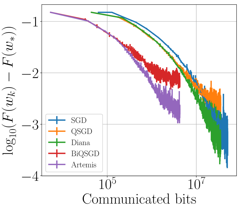
(a) Quantum

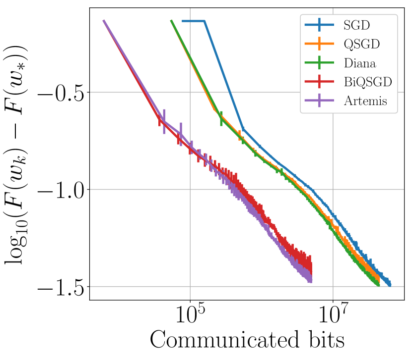
(b) Superconduct

Figure 3: Partial participation - PP1 (non-i.i.d.): $\sigma_{*}=0$ (same experiments in stochastic regime: Figure S16), $N=20$ workers, $p=0.5$, $b>1$ ($400$ iter.). X-axis in # bits.

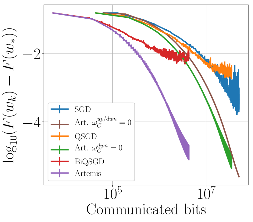
(a) Quantum

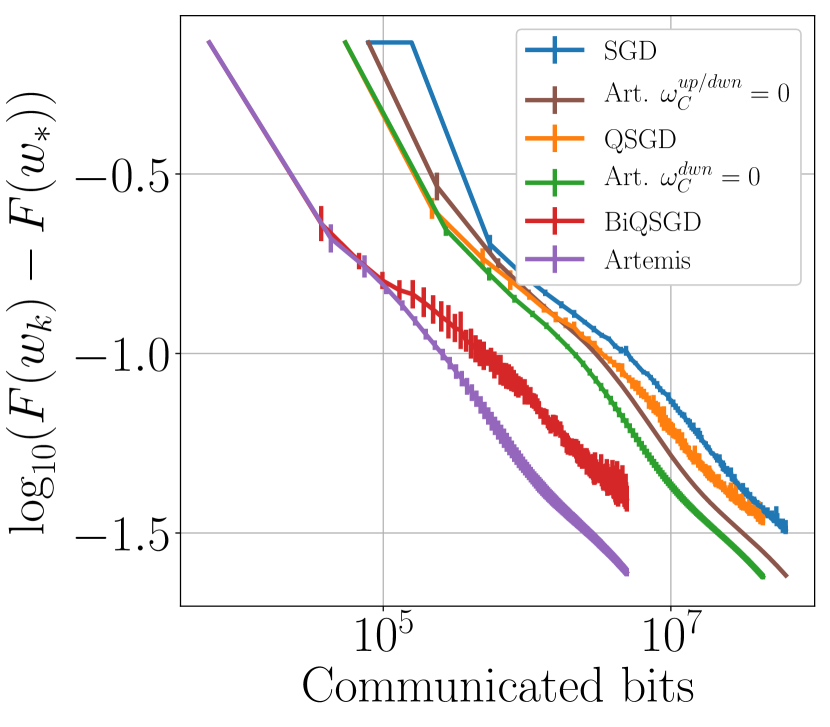
(b) Superconduct

Figure 4: Partial participation - PP2 (non-i.i.d.): $\sigma_{*}=0$ (same experiments in stochastic regime: Figure S17), $N=20$ workers, $p=0.5$, $b>1$ ($400$ iter.). X-axis in # bits.

Heterogeneity and real datasets. While in Figure 1(a), data is i.i.d. on machines, and Artemis is thus not expected to outperform Bi-QSGD (the difference between the two being the memory), in Figures 4, 3, 2 and 1(b) we use non-i.i.d. data. None of the previous papers on compression directly illustrated the impact of heterogeneity on simple examples, neither compared it with i.i.d. situations.

Partial participation. On Figures 4 and 3 we run experiments with only half of the devices active (randomly sampled) at each iteration with the two approaches (PP1 and PP2) described in Section 4 in a full gradient regime (same experiments in stochastic regime are given in Subsection C.2.1). This two figures emphasize the failure of the first approach PP1 compared to PP2. We observe that in this last case only, Artemis has a linear convergence. It also stresses the key role of the memory in this setting. On Figure 4, all algorithms with a (single) memory (with or without up/down compression) are better than SGD without memory. Note that Diana is defined with multiple memories, thus it cannot be compared to Artemis with PP2.

6 Conclusion

We propose Artemis, a framework using bidirectional compression to reduce the number of bits needed to perform distributed or federated learning. On top of compression, Artemis includes a memory mechanism which improves convergence over non-i.i.d. data. As PP is a classical setting, we designed an approach (PP2) to tackle it while leveraging the full impact of memory, outperforming existing solutions. We provide three tight theorems giving guarantees of a fast convergence (linear up to a threshold), highlighting the impact of memory, analyzing Polyak-Ruppert averaging and obtaining lowers bound by studying convergence in distribution of our algorithm. Altogether, this improves the understanding of compression combined with a memory mechanism and sheds light on challenges ahead.

Appendix A Additional details about the Artemis framework

The aim of this section is threefold. First, we give the pseudo-code of Artemis. Secondly, we provide supplementary details about the quantization scheme used in our work. We also explain (based on Alistarh et al. [2017]) how quantization combined with Elias code [see Elias, 1975] reduces the required number of bits to send information. Thirdly, we define the filtrations used in our proofs and give their resulting properties.

A.1 Artemis pseudo-code

We provide the pseudo-code of Artemis in Algorithm 1 and for the understanding of Artemis implementation, we give a visual illustration of the algorithm in Figure S1.

Remark 3.

Remark that we have used in Algorithm 1 the true value of $p$ in the update (to get an unbiased estimator of the gradient), but it is obviously possible to use an estimated value $\hat{p}$ in Equation 6: indeed, it is exactly equivalent to multiplying the step size $\gamma$ by a factor $p/\hat{p}$, thus neither changes the practical implementation nor the theoretical analysis.

Input: Mini-batch size $b$, learning rates $\alpha,\gamma>0$, initial model $w_{0}\in\mathbb{R}^{d}$, operators $\mathcal{C}_{\mathrm{up}}$ and $\mathcal{C}_{\mathrm{dwn}}$, $M_{1}$ and $M_{2}$ the sizes of the full/compressed gradients.

Initialization: Local memory: $\forall i\in\llbracket 1,N\rrbracket$ $h_{0}^{i}=0$ (kept on both central server and device $i$). Index of last participation: $k_{i}=0$.

Output: Model $w_{K}$

for $k=0,1,2,\dots,K$ do

       Randomly sample a set of device $S_{k}$

       for each device $i\in S_{k}$ do

             Catching up.

             If $k-k_{i}$ > $\lfloor M_{1}/M_{2}\rfloor$, send the model $w_{k}$

             Else send $(\widehat{\Omega}_{j})_{j=k_{i}+1}^{k}$ and update local model: $\forall j\in\llbracket k_{i}+1,k\rrbracket,\quad w_{j}=w_{j-1}-\gamma\Omega_{j,S_{j-1}}$

             Update index of its last participation: $k_{i}=k$

             Local training.

             Compute stochastic gradient $g_{k+1}^{i}=\textsl{g}_{k+1}(w_{k})$ (with mini-batch)

             Set $\Delta_{k}^{i}=g_{k+1}^{i}-h_{k}^{i}$, compress it $\widehat{\Delta}_{k}^{i}=\mathcal{C}_{\mathrm{up}}(\Delta_{k}^{i})$

             Update memory term: $h_{k+1}^{i}=h_{k}^{i}+\alpha\widehat{\Delta}_{k}^{i}$

             Send $\widehat{\Delta}_{k}^{i}$ to central server

            

      Compute $\widehat{g}_{k+1,S_{k}}=h_{k}+\frac{\displaystyle 1}{\displaystyle pN}\sum_{i\in S_{k}}\widehat{\Delta}_{k}^{i}$

       Update central memory: $h_{k+1}=h_{k}+\alpha\frac{\displaystyle 1}{\displaystyle N}\sum_{i\in S_{k}}\widehat{\Delta}_{k}^{i}$

       Back compression: $\Omega_{k+1,S_{k}}=\mathcal{C}_{\mathrm{dwn}}(\widehat{g}_{k+1,S_{k}})$

       Broadcast $\Omega_{k+1}$ to all workers.

       Update model on central server: $w_{k+1}=w_{k}-\gamma\Omega_{k+1,S_{k}}$

      

Algorithm 1 Artemis - set $\alpha>0$ to use memory.

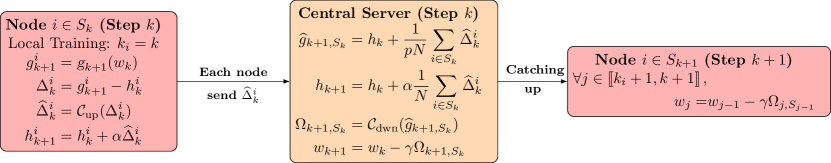
Figure S1: Visual illustration of Artemis bidirectional compression at iteration $k\in\mathbb{N}$. $w_{k}$ is the model’s parameter, $\mathcal{C}_{\mathrm{up}}$ and $\mathcal{C}_{\mathrm{dwn}}$ are the compression operators, $\gamma$ is the step size, $\alpha$ is the learning rate which simulates a memory mechanism of past iterates and allows the compressed values to tend to zero.

A.2 Quantization scheme

In the following, we define the $s$-quantization operator $\mathcal{C}_{s}$ which we use in our experiments. After giving its definition, we explain [based on Alistarh et al., 2017] how it helps to reduce the number of bits to broadcast.

Definition 1 ($s$-quantization operator).

Given $\Delta\in\mathbb{R}^{d}$, the $s$-quantization operator $\mathcal{C}_{s}$ is defined by:

$$\mathcal{C}_{s}(\Delta):=sign(\Delta)\times\|\Delta\|_{2}\times\frac{\psi}{s}\,.$$

$\psi\in\mathbb{R}^{d}$ is a random vector with $j$-th element defined as:

$$\psi_{j}:=\left\{\begin{array}[]{ll}l+1&\mbox{with probability }s\frac{|\Delta_{j}|}{\|\Delta\|_{2}}-l\\ l&\mbox{otherwise}\,.\end{array}\right.$$

where the level $l$ is such that $\frac{\displaystyle\Delta_{i}}{\displaystyle\left\|\Delta\right\|_{2}}\in\left[\frac{\displaystyle l}{\displaystyle s},\frac{\displaystyle l+1}{\displaystyle s}\right]$.

The $s$-quantization scheme verifies Assumption 5 with $\omega_{\mathcal{C}}=\min(d/s^{2},\sqrt{d}/s)$. Proof can be found in [Alistarh et al., 2017, see Appendix A.1].

Now, for any vector $v\in\mathbb{R}^{d}$, we are in possession of the tuple $(\|v\|^{2},\phi,\psi)$, where $\phi$ is the vector of signs of $(v_{i})_{i=1}^{d}$, and $\psi$ is the vector of integer values $(\psi_{j})_{j=1}$. To broadcast the quantized value, we use the Elias encoding Elias [1975]. Using this encoding scheme, it can be shown (Theorem 3.2 of Alistarh et al. [2017]) that:

Proposition S1.

For any vector $v$, the number of bits needed to communicate $\mathcal{C}_{s}(v)$ is upper bounded by:

$$\left(3+\left(\frac{3}{2}+o(1)\right)\log\left(\frac{2(s^{2}+d)}{s(s+\sqrt{d})}\right)\right)s(s+\sqrt{d})+32\,.$$

The final goal of using memory for compression is to quantize vectors with $s=1$. It means that we will employ $O(\sqrt{d}\log d)$ bits per iteration instead of $32d$, which reduces by a factor $\frac{\sqrt{d}}{\log d}$ the number of bits used by iteration. Now, in a FL settings, at each iteration we have a double communication (device to the main server, main server to the device) for each of the $N$ devices. It means that at each iteration, we need to communicate $2\times N\times 32d$ bits if compression is not used. With a single compression process like in Mishchenko et al. [2019]; Li et al. [2020]; Wu et al. [2018]; Agarwal et al. [2018]; Alistarh et al. [2017], we need to broadcast

$$O\left(32Nd+N\sqrt{d}\log d\right) =O\left(Nd\left(1+\frac{\log d}{\sqrt{d}}\right)\right)$$

$$=O\left(Nd\right)\,.$$

But with a bidirectional compression, we only need to broadcast $O\left(2N\sqrt{d}\log d\right)$.

Time complexity analysis of simple vs double compression for the $1$-quantization schema.

Using quantization with $s=1$, and then the Elias code [defined in Elias, 1975] to communicate between servers, leads to reduce from $O(Nd)$ to $O(N\sqrt{d}\log(d))$ the number of bits to send, for each direction. Getting an estimation of the total time complexity is difficult and inevitably dependant of the considered application. Indeed, as highlighted by Figure S3, download and upload speed are always different. The biggest measured difference between upload and download is found in Europa for mobile broadband ; their ratio is around $3.5$.

Denoting $v_{d}$ and $v_{u}$ the speed of download and upload (in bits per second), we typically have $v_{d}=\rho v_{u}$, $3.5>\rho>1$.

Then for unidirectional compression, each iteration takes $O\left(\frac{Nd}{v_{d}}+\frac{N\sqrt{d}\log(d)}{v_{u}}\right)\approx O\left(\frac{Nd}{\rho v_{u}}\right)$ seconds, while for a bidirectional one it takes only $O\left(\frac{N\sqrt{d}\log(d)}{v_{d}}+\frac{N\sqrt{d}\log(d)}{v_{u}}\right)\approx O\left(\frac{N\sqrt{d}\log(d)}{v_{u}}\right)$ seconds.

In other words, unless $\rho$ is really large (which is not the case in practice as stressed by Figure S3, double compression reduces by several orders of magnitude the global time complexity, and bidirectional compression is by far superior to unidirectional.

A.3 Filtrations

In this section we provide some explanations about filtrations - especially a rigorous definition - and how it is used in the proofs of Theorems 2, 3, S5 and S6. We recall that we denoted by $\omega_{\mathcal{C}}^{\mathrm{up}}$ and $\omega_{\mathcal{C}}^{\mathrm{dwn}}$ the variance factors for respectively uplink and downlink compression.

Let a probability space $(\Omega,\mathcal{A},\mathbb{P})$ with $\Omega$ a sample space, $\mathcal{A}$ an event space, and $\mathbb{P}$ a probability function. We recall that the $\sigma$-algebra generated by a random variable $X:\Omega\rightarrow\mathbb{R}^{m}$ is

$$\sigma(X)=\{X^{-1}(A):A\in\mathcal{B}(\mathbb{R}^{m})\}\,,$$

where $\mathcal{B}(\mathbb{R}^{m})$ is the Borel set of $\mathbb{R}^{m}$.

Furthermore, we recall that a filtration of $(\Omega,\mathcal{F},P)$ is defined as an increasing sequence $(\mathcal{F}_{n})_{n\in\mathbb{N}}$ of $\sigma$-algebras:

$$\mathcal{F}_{0}\subset\mathcal{F}_{1}\subset\mathcal{F}_{2}\subset\dots\subset\mathcal{F}\,.$$

Concerning randomness in our algorithm, it comes from four sources:

1. Stochastic gradients. It corresponds to the noise associated with the stochastic gradients computation on device $i$ at epoch $k$. We have:

   $$\forall k\in\mathbb{N}\,,\leavevmode\nobreak\ \forall i\in\llbracket 0,...,N\rrbracket,\quad g_{k+1}^{i}=\nabla F_{i}(w_{k})+\xi_{k+1}^{i}(w_{k})\,,\text{ with $\mathbb{V}(\xi_{k+1}^{i})$ bounded.}$$

2. Uplink compression: this noise corresponds to the uplink compression when local gradients are compressed. Let $k\in\mathbb{N}$ and $i\in\llbracket 0,...,N\rrbracket$, suppose, we want to compress $\Delta_{k}^{i}\in\mathbb{R}^{d}$, then the associated noise is $\epsilon_{k+1}^{i}$ with $\mathbb{V}(\epsilon_{k+1}^{i}(\Delta_{k}^{i}))\leq\omega_{\mathcal{C}}^{\mathrm{up}}\left\|\Delta_{k}^{i}\right\|^{2}$, where $\omega_{\mathcal{C}}^{\mathrm{up}}\in\mathbb{R}^{*}$ is defined by the uplink compression schema (see Assumption 5). And it follows that:

   $$\forall k\in\mathbb{N},\leavevmode\nobreak\ \forall i\in\llbracket 0,...,N\rrbracket,\quad\widehat{\Delta}_{k}^{i}=\Delta_{k}^{i}+\epsilon_{k}^{i}(\Delta_{k}^{i})\Longleftrightarrow\widehat{g}_{k+1}^{i}=g_{k+1}^{i}+\epsilon_{k+1}^{i}(\Delta_{k}^{i})\,.$$

3. Downlink compression. This noise corresponds to the downlink compression, when the global model parameter is compressed. Let $k\in\mathbb{N}$, suppose we want to compress $\widehat{g}_{k+1,S_{k}}\in\mathbb{R}^{d}$, then the associated noise is $\epsilon_{k+1}(\widehat{g}_{k+1,S_{k}})$ with $\mathbb{V}(\epsilon_{k+1})\leq\omega_{\mathcal{C}}^{\mathrm{dwn}}\left\|\widehat{g}_{k+1,S_{k}}\right\|^{2}$. There is:

   $$\forall k\in\mathbb{N},\quad\Omega_{k+1,S_{k}}=\mathcal{C}_{s}(\widehat{g}_{k+1,S_{k}})=\widehat{g}_{k+1,S_{k}}+\epsilon_{k+1}(\widehat{g}_{k+1,S_{k}})\,.$$

4. Random sampling. This randomness corresponds to the partial participation of each device. We recall that according to Assumption 6, each device has a probability $p$ of being active. For $k$ in $\mathbb{N}$, for $i$ in $\llbracket 1,N\rrbracket$, we note $B_{k}^{i}\sim\mathcal{B}(p)$ the Bernoulli random variable that marks if a device is active or not at step $k$.

${w_{k}\xrightarrow{\quad{\xi_{k+1}^{i}}\quad}g_{k+1}^{i}\xrightarrow{\quad{\epsilon_{k+1}^{i}}\quad}\widehat{g}_{k+1}^{i}\xrightarrow{\quad{B_{k}^{i}}\quad}\widehat{g}_{k+1,S_{k}}=\sum_{i\in S_{k}}\widehat{g}_{k+1}^{i}\xrightarrow{\quad{\epsilon_{k+1}}\quad}\Omega_{k+1,S_{k}}=\mathcal{C}\left(\widehat{g}_{k+1,S_{k}}\right)}$

Figure S2: The sequence of successive additive noises in the algorithm.

This “succession of noises” in the algorithm is illustrated in Figure S2. In order to handle these four sources of randomness, we define five sequences of nested $\sigma$-algebras.

Definition 2.

We note $(\mathcal{F}_{k})_{k\in\mathbb{N}}$ the filtration associated to the stochastic gradient computation noise, $(\mathcal{G}_{k})_{k\in\mathbb{N}}$ the filtration associated to the uplink compression noise and $(\mathcal{H}_{k})_{k\in\mathbb{N}}$ the filtration associated to the downlink compression noise, $(\mathcal{B}_{k})_{k\in\mathbb{N}}$ the filtration associated to the random device participation randomness. For $k\in\mathbb{N}^{*}$, we define:

$$\mathcal{F}_{k} =\sigma\left(\Gamma_{k-1},(\xi_{k}^{i})_{i=1}^{N}\right)$$

$$\mathcal{G}_{k} =\sigma\left(\Gamma_{k-1},(\xi_{k}^{i})_{i=1}^{N},(\epsilon_{k}^{i})_{i=1}^{N}\right)$$

$$\mathcal{H}_{k} =\sigma\left(\Gamma_{k-1},(\xi_{k}^{i})_{i=1}^{N},(\epsilon_{k}^{i})_{i=1}^{N},\epsilon_{k}\right)$$

$$\mathcal{B}_{k-1} =\sigma\left((B_{k-1}^{i})_{i=1}^{N}\right)$$

$$\mathcal{I}_{k} =\sigma\left(\mathcal{H}_{k}\cup\mathcal{B}_{k-1}\right)\,,$$

with

$$\Gamma_{k}=\{(\xi_{t}^{i})_{i\in\llbracket 1,N\rrbracket},(\epsilon_{t}^{i})_{i\in\llbracket 1,N\rrbracket},\epsilon_{t},(B_{k-1}^{i})_{i=1}^{N}\}_{t\in\llbracket 1,k\rrbracket}\text{\quad and \quad}\Gamma_{0}=\{\varnothing\}\,.$$

We can make the following observations for all $k\geq 1$:

• From these three definitions, it follows that our sequences are nested.

  $$\mathcal{F}_{1}\subset\mathcal{G}_{1}\subset\mathcal{H}_{1}\subset\mathcal{F}_{2}\subset\dots\subset\mathcal{H}_{K}\,.$$

  However, $(\mathcal{B}_{k})_{k\in\mathbb{N}}$ is independent of the other filtrations.

• $\mathcal{I}_{k}=\sigma\left(\mathcal{H}_{k}\cup\mathcal{B}_{k-1}\right)=\sigma(\Gamma_{k})$, and the aim is to express the expectation w.r.t. all randomness i.e $\mathcal{I}_{k}$.

• $w_{k}$ is $\mathcal{I}_{k}$-measurable.

• $g_{k+1}(w_{k})$ is $\mathcal{F}_{k+1}$-measurable.

• $\widehat{g}_{k+1}(w_{k})$ is $\mathcal{G}_{k+1}$-measurable.

• $B_{k-1}^{i}$ is $\mathcal{B}_{k-1}$-measurable.

• $g_{k+1,S_{k}}\,,\widehat{g}_{k+1,S_{k}}$ and $\Omega_{k+1,S_{k}}$ are respectively $\sigma(\mathcal{F}_{k+1}\cup\mathcal{B}_{k})$-measurable, $\sigma(\mathcal{G}_{k+1}\cup\mathcal{B}_{k})$-measurable and $\sigma(\mathcal{H}_{k+1}\cup\mathcal{B}_{k})$-measurable. Note that $\mathcal{F}_{k+1}$ contains $\Gamma_{k}$, and thus all $(B_{k-1}^{i})^{N}_{i=1}$, but does not contain all the $(B_{k}^{i})^{N}_{i=1}$.

As a consequence, we have Propositions S2, S3, S4, S5, S6, S7 and S8. Please, take notice that for sake of clarity Propositions S2, S3, S4, S5 and S6 are stated without taking into account the random participation $S_{k}$. All this proposition remains identical when adding partial participation, the results only have to be expressed w.r.t. active nodes $S_{k}$.

Below Proposition S2 gives the expectation over stochastic gradients conditionally to $\sigma$-algebras $\mathcal{H}_{k}$ and $\mathcal{F}_{k+1}$.

Proposition S2 (Stochastic Expectation).

Let $k\in\mathbb{N}$ and $i\in\llbracket 1,N\rrbracket$. Then on each local device $i\in\llbracket 1,N\rrbracket$ we have almost surely (a.s.):

$$\left\{\begin{array}[]{ll}\mathbb{E}\left[g_{k+1}^{i}\leavevmode\nobreak\ \middle|\leavevmode\nobreak\ \mathcal{F}_{k+1}\right]&=g_{k+1}^{i}\\ \mathbb{E}\left[g_{k+1}^{i}\leavevmode\nobreak\ \middle|\leavevmode\nobreak\ \mathcal{H}_{k}\right]&=\nabla F_{i}(w_{k})\,,\end{array}\right.$$

which leads to:

$$\left\{\begin{array}[]{ll}\mathbb{E}\left[g_{k+1}\leavevmode\nobreak\ \middle|\leavevmode\nobreak\ \mathcal{F}_{k+1}\right]&=g_{k+1}\\ \mathbb{E}\left[g_{k+1}\leavevmode\nobreak\ \middle|\leavevmode\nobreak\ \mathcal{H}_{k}\right]&=\nabla F(w_{k})\,.\end{array}\right.$$

Proposition S3 gives expectation of uplink compression (information sent from remote devices to central server) conditionally to $\sigma$-algebras $\mathcal{F}_{k+1}$ and $\mathcal{G}_{k+1}$.

Proposition S3 (Uplink Compression Expectation).

Let $k\in\mathbb{N}$ and $i\in\llbracket 1,N\rrbracket$. Recall that $\widehat{g}_{k}^{i}=g_{k}^{i}+\epsilon_{k}^{i}$, then on each local device $i\in\llbracket 1,N\rrbracket$, we have a.s:

$$\left\{\begin{array}[]{ll}\mathbb{E}\left[\widehat{g}_{k+1}^{i}\leavevmode\nobreak\ \middle|\leavevmode\nobreak\ \mathcal{G}_{k+1}\right]=\widehat{g}_{k+1}^{i}\\ \mathbb{E}\left[\widehat{g}_{k+1}^{i}\leavevmode\nobreak\ \middle|\leavevmode\nobreak\ \mathcal{F}_{k+1}\right]=g_{k+1}^{i}\,,\end{array}\right.$$

which leads to

$$\left\{\begin{array}[]{l}\mathbb{E}\left[\widehat{g}_{k+1}\leavevmode\nobreak\ \middle|\leavevmode\nobreak\ \mathcal{G}_{k+1}\right]=\widehat{g}_{k+1}\\ \mathbb{E}\left[\widehat{g}_{k+1}\leavevmode\nobreak\ \middle|\leavevmode\nobreak\ \mathcal{F}_{k+1}\right]=\mathbb{E}\left[\frac{1}{N}\sum_{i=1}^{N}\widehat{g}_{k+1}^{i}\leavevmode\nobreak\ \middle|\leavevmode\nobreak\ \mathcal{F}_{k+1}\right]=g_{k+1}\,.\\ \end{array}\right.$$

From Assumption 5, if follows that variance over uplink compression can be bounded as expressed in Proposition S4.

Proposition S4 (Uplink Compression Variance).

Let $k\in\mathbb{N}$ and $i\in\llbracket 1,N\rrbracket$. Recall that $\Delta_{k}^{i}=g_{k+1}^{i}+h_{k}^{i}$, using Assumption 5 following hold a.s:

$$\mathbb{E}\left[\|\widehat{\Delta}_{k+1}^{i}-\Delta_{k+1}^{i}\|^{2}\leavevmode\nobreak\ \middle|\leavevmode\nobreak\ \mathcal{F}_{k+1}\right]\leq\omega_{\mathcal{C}}^{\mathrm{up}}\|\Delta_{k+1}^{i}\|^{2}$$ (S1)

$$(\Longleftrightarrow\qquad \mathbb{E}\left[\|\widehat{g}_{k+1}^{i}-g_{k+1}^{i}\|^{2}\leavevmode\nobreak\ \middle|\leavevmode\nobreak\ \mathcal{F}_{k+1}\right]\leq\omega_{\mathcal{C}}^{\mathrm{up}}\|g_{k+1}^{i}\|^{2}\text{ when no memory })\,.$$ (S2)

Concerning downlink compression (information sent from central server to each node), Proposition S5 gives its expectation w.r.t $\sigma$-algebras $\mathcal{G}_{k+1}$ and $\mathcal{H}_{k+1}$.

Proposition S5 (Downlink Compression Expectation).

Let $k\in\mathbb{N}$, recall that $\Omega_{k+1}=\mathcal{C}_{\mathrm{dwn}}(\widehat{g}_{k+1})=\widehat{g}_{k+1}+\epsilon_{k}$, then a.s:

$$\left\{\begin{array}[]{ll}\mathbb{E}\left[\Omega_{k+1}\leavevmode\nobreak\ \middle|\leavevmode\nobreak\ \mathcal{H}_{k+1}\right]=\Omega_{k+1}\\ \mathbb{E}\left[\Omega_{k+1}\leavevmode\nobreak\ \middle|\leavevmode\nobreak\ \mathcal{G}_{k+1}\right]=\widehat{g}_{k+1}\,.\end{array}\right.$$

Next proposition states that downlink compression can be bounded as for Proposition S4.

Proposition S6 (Downlink Compression Variance).

Let $k\in\mathbb{N}$, using Assumption 5 following holds a.s:

$$\mathbb{E}\left[\|\Omega_{k+1}-\widehat{g}_{k+1}\|^{2}\leavevmode\nobreak\ \middle|\leavevmode\nobreak\ \mathcal{G}_{k+1}\right]\leq\omega_{\mathcal{C}}^{\mathrm{dwn}}\|\widehat{g}_{k+1}\|^{2}\,.$$

Now, we give in Propositions S8 and S7 the expectation and the variance w.r.t. devices random sampling noise.

Proposition S7 (Expectation of device sampling).

Let $k\in\mathbb{N}$, let’s note $a_{k+1}=\frac{1}{N}\sum_{i=1}^{N}a_{k+1}^{i}$ and $a_{k+1,S_{k}}=\frac{1}{pN}\sum_{i\in S_{k}}a_{k+1}^{i}$, where $(a_{k+1}^{i})_{i=0}^{N}\in(\mathbb{R}^{d})^{N}$ are $N$ random variables independent of each other and $\mathcal{J}_{k+1}$-measurable, for a $\sigma$-field $\mathcal{J}_{k+1}$ s.t. $(B_{k}^{i})^{N}_{i=1}$ are independent of $\mathcal{J}_{k+1}$. We have a.s:

$$\mathbb{E}\left[a_{k+1,S_{k}}\leavevmode\nobreak\ \middle|\leavevmode\nobreak\ \mathcal{J}_{k+1}\right]=a_{k+1}\,.$$

The vector $a_{k+1}$ (resp. the $\sigma$-field $\mathcal{J}_{k+1}$) may represent various objects, for instance : $g_{k+1}$, $\widehat{g}_{k+1}$, $\Omega_{k+1}$ (resp. $\mathcal{F}_{k+1}$, $\mathcal{G}_{k+1}$, $\mathcal{H}_{k+1}$).

Proof.

For any $k\in\mathbb{N}^{*}$, we have that:

$$\mathbb{E}\left[a_{k+1,S_{k}}\leavevmode\nobreak\ \middle|\leavevmode\nobreak\ \mathcal{J}_{k+1}\right] =\mathbb{E}\left[\frac{1}{pN}\sum_{i\in S_{k}}a_{k+1}^{i}\leavevmode\nobreak\ \middle|\leavevmode\nobreak\ \mathcal{J}_{k+1}\right]=\mathbb{E}\left[\frac{1}{pN}\sum_{i=0}^{N}a_{k+1}^{i}B^{i}_{k}\leavevmode\nobreak\ \middle|\leavevmode\nobreak\ \mathcal{J}_{k+1}\right]$$

$$=\frac{1}{pN}\sum_{i=0}^{N}\mathbb{E}\left[a_{k+1}^{i}B_{k}^{i}\leavevmode\nobreak\ \middle|\leavevmode\nobreak\ \mathcal{J}_{k+1}\right]\text{ by linearity of the expectation,}$$

$$=\frac{1}{pN}\sum_{i=0}^{N}a_{k+1}^{i}\mathbb{E}\left[B_{k}^{i}\leavevmode\nobreak\ \middle|\leavevmode\nobreak\ \mathcal{J}_{k+1}\right]\text{because $(a_{k+1}^{i})^{N}_{i=1}$ are $\mathcal{J}_{k+1}$-measurable,}$$

$$=\frac{1}{N}\sum_{i=0}^{N}a_{k+1}^{i}=a_{k+1}\,\text{because $(B_{k}^{i})^{N}_{i=1}$ are independent of $\mathcal{J}_{k+1}$,}$$

which allows to conclude. ∎

Proposition S8 (Variance of device sampling).

Let $k\in\mathbb{N}^{*}$, with the same notation as Proposition S7, we have a.s:

$$\mathbb{V}\left[a_{k+1,S_{k}}\leavevmode\nobreak\ \middle|\leavevmode\nobreak\ \mathcal{J}_{k+1}\right]=\frac{\displaystyle 1-p}{\displaystyle pN^{2}}\sum_{i=0}^{N}\left\|a_{k+1}^{i}\right\|^{2}\,.$$

Proof.

Let $k\in\mathbb{N}^{*}$,

$$\mathbb{V}\left[a_{k+1,S_{k}}\leavevmode\nobreak\ \middle|\leavevmode\nobreak\ \mathcal{J}_{k+1}\right] =\mathbb{V}\left[\frac{1}{pN}\sum_{i=0}^{N}a_{k+1}^{i}B^{i}_{k}\leavevmode\nobreak\ \middle|\leavevmode\nobreak\ \mathcal{J}_{k+1}\right]$$

$$=\frac{1}{p^{2}N^{2}}\sum_{i=0}^{N}\mathbb{V}\left[a_{k+1}^{i}B_{k}^{i}\leavevmode\nobreak\ \middle|\leavevmode\nobreak\ \mathcal{J}_{k+1}\right]\text{because $(B_{k}^{i})^{N}_{i=1}$ are independent,}$$

$$=\frac{1}{p^{2}N^{2}}\sum_{i=0}^{N}\left\|a_{k+1}^{i}\right\|^{2}\mathbb{V}\left[B_{k}^{i}\leavevmode\nobreak\ \middle|\leavevmode\nobreak\ \mathcal{J}_{k+1}\right]\text{because $(a_{k+1}^{i})^{N}_{i=1}$ are $\mathcal{J}_{k+1}$-measurable,}$$

$$=\frac{\displaystyle 1-p}{\displaystyle pN^{2}}\sum_{i=0}^{N}\left\|a_{k+1}^{i}\right\|^{2}\,\text{because $(B_{k}^{i})^{N}_{i=1}$ are independent of $\mathcal{J}_{k+1}$.}$$

∎

Appendix B Bandwidth speed

In a network configuration where download would be much faster than upload, bidirectional compression would present no benefit over unidirectional, as downlink communications would have a negligible cost. However, this is not the case in practice: to assess this point, we gathered broadband speeds, for both download and upload communications, for fixed broadband (cable, T1, DSL …) or mobile (cellphones, smartphones, tablets, laptops …) from studies carried out in $2020$ over the $6$ continents by Speedtest.net [see noa, ]. Results are provided in Figure S3, comparing download and upload speeds. The ratios (averaged by continents) between upload and download speeds stand between $1$ (in Asia, for fixed broadband) and $3.5$ (in Europe, for mobile broadband): there is thus no apparent reason to simply disregard the downlink communication, and bi-directionnal compression is unavoidable to achieve substantial speedup. More precisely, if we denote $v_{d}$ and $v_{u}$ the speed of download and upload (in Mbits per second), we typically have $v_{d}=\rho v_{u}$, with $1<\rho<3.5$. Using quantization with $s=1$ (see Subsection A.2), for unidirectional compression, each iteration takes $O\left(\frac{Nd}{\rho v_{u}}\right)$ seconds, while for a bidirectional one it takes only $O\left(\frac{N\sqrt{d}\log(d)}{v_{u}}\right)$ seconds.

The dataset is pickled from a study carried out by Speedtest.net [see noa, ]. This study has measured the bandwidth speeds in 2020 accross the six continents. In order to get a better understanding of this dataset, we illustrate the speeds distribution on Figures S3, S5, 4(a) and 4(b).

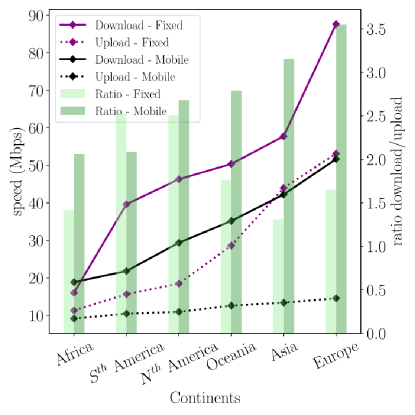
Figure S3: Left axis: upload and download speed for mobile and fixed broadband. Left axis: speeds (in Mbps), right axis: ratio (green bars). The dataset is gathered from Speedtest.net, see noa .

In Figures S5, 4(a) and 4(b), unlike Figure S3, we do not aggregate data by countries of a same continents. This allows to analyse the speeds ratio between upload and download with the proper value of each countries. Looking at Figures 4(a), 4(b) and S5, it is noticeable that in the world, the ratio between upload and download speed is between $1$ and $5$, and not between $1$ and $3.5$ as Figure S3 was suggesting since we were aggregating data by continents. There are only nine countries in the world having a ratio higher than $5$. In Europe : Malta, Belgium and Montenegro. In Asia : South Korea. In North America : Canada, Saint Vincent and the Grenadines, Panama and Costa Rica. In Africa : Western Sahara. The highest ratio is $7.7$ observed in Malta.

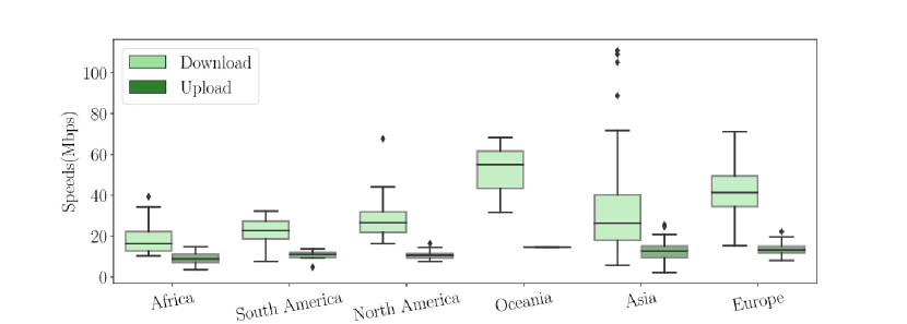
(a) Mobile broadband.

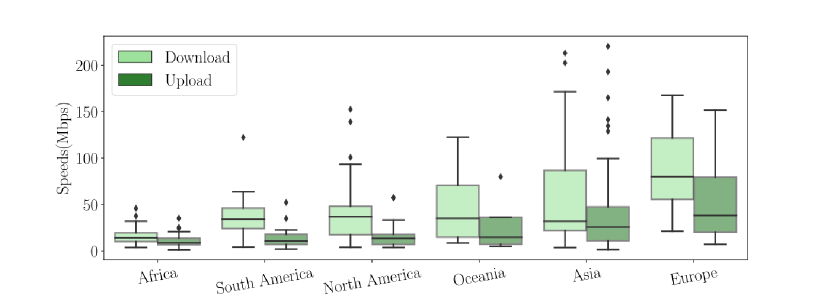
(b) Fixed broadband.

Figure S4: Upload/download speed (in Mbps). Best seen incolors.

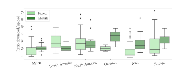
Figure S5: Distribution of the download/upload speeds ratio by continents. Best seen in colors.

Appendix C Experiments

In this section we provide additional details about our experiments. We recall that we use two kind of datasets: 1) toy-ish synthetic datasets and 2) real datasets: superconduct [see Hamidieh, 2018, 21263 points, 81 features] and quantum [see Caruana et al., 2004, 50,000 points, 65 features]. The aim of using synthetic datasets is mainly to underline the properties resulting from Theorems 3, 1 and 2.

We use the same $1$-quantization scheme (defined in Subsection A.2, $s=1$ is the most drastic compression) for both uplink and downlink, and thus, we consider that $\omega_{\mathcal{C}}^{\mathrm{up}}=\omega_{\mathcal{C}}^{\mathrm{dwn}}$. In addition, we choose $\alpha^{\mathrm{up}}=\alpha^{\mathrm{dwn}}=\frac{\displaystyle 1}{\displaystyle 2(1+\omega_{\mathcal{C}}^{\mathrm{up}/\mathrm{dwn}})}$.

For each figure, we plot the convergence w.r.t. the number of iteration $k$ or w.r.t. the theoretical number of bits exchanged after $k$ iterations. On the Y-axis we display $\log_{10}(F(w_{k})-F(w_{*}))$, with $k$ in $\mathbb{N}$. All experiments have been run $5$ times and averaged before displaying the curves. We plot error bars on all figures. To compute error bars we use the standard deviation of the logarithmic difference between the loss function at iteration $k$ and the objective loss, that is we take standard deviation of $\log_{10}(F(w_{k})-F(w_{*}))$. We then plot the curve $\pm$ this standard deviation.

All the code is available in supplementary material.

C.1 Synthetic dataset

We build two different synthetic dataset for i.i.d. or non-i.i.d. cases. We use linear regression to tackle the i.i.d case and logistic regression to handle the non-i.i.d. settings. As explained in Section 1, each worker $i$ holds $n_{i}$ observations $(z_{j}^{i})_{1\leq j\leq n_{i}}=(x_{j}^{i},y_{j}^{i})_{1\leq j\leq n_{i}}=(X^{i},Y^{i})$ following a distribution $D_{i}$.

We use $N=10$ devices, each holding $200$ points of dimension $d=20$ for least-square regression and $d=2$ for logistic regression. We ran algorithms over $100$ epochs.

Choice of the step size for synthetic dataset.

For stochastic descent, we use a step size $\gamma=\frac{1}{L\sqrt{k}}$ with $k$ the number of iteration, and for the batch descent we choose $\gamma=\frac{1}{L}$.

For i.i.d. setting, we use a linear regression model without bias. For each worker $i$, data points are generated from a normal distribution $(x_{j}^{i})_{1\leq j\leq n_{i}}\sim\mathcal{N}(0,\Sigma)$. And then, for all $j$ in $\llbracket 1,n_{i}\rrbracket$, we have: $y_{j}^{i}=\left\langle w\leavevmode\nobreak\ \middle|\leavevmode\nobreak\ x_{j}^{i}\right\rangle+e_{i}$ with $e_{i}\sim\mathcal{N}(0,\lambda^{2})$ and $w$ the true model.

To obtain $\sigma_{*}=0$, it is enough to remove the noise $e_{i}$ by setting the variance $\lambda^{2}$ of the dataset distribution to $0$. Indeed, using a least-square regression, for all $i$ in $\llbracket 1,N\rrbracket$, the cost function evaluated at point $w$ is $F_{i}(w)=\frac{1}{2}\|{{X^{i}}^{T}w-Y^{i}}\|^{2}$. Thus the stochastic gradient $j$ in $\llbracket 1,n_{i}\rrbracket$ on device $i$ in $\llbracket 1,N\rrbracket$ is $\textsl{g}_{j}^{i}(w)=({X^{i}_{j}}^{T}w-Y^{i}_{j})X^{i}_{j}$. On the other hand, the true gradient is $\nabla F_{i}(w)=\mathbb{E}X^{i}{X^{i}}^{T}(w-w^{*})$. Computing the difference, we have for all device $i$ in $\llbracket 1,N\rrbracket$ and all $j$ in $\llbracket 1,n_{i}\rrbracket$:

$$\textsl{g}_{j}^{i}(w)-F_{i}(w)=\underbrace{(X^{i}_{j}{X^{i}_{j}}^{T}-\mathbb{E}X^{i}{X^{i}}^{T})(w-w_{*})}_{\text{multiplicative noise equal to }0\text{ in }w_{*}}+\underbrace{({X^{i}_{j}}^{T}w_{*}-Y_{j}^{i})}_{\sim\mathcal{N}(0,\lambda^{2})}X^{i}_{j}$$ (S3)

This is why, if we set $\lambda=0$ and evaluate eq. S3 at $w_{*}$, we get back Assumption 3 with $\sigma_{*}=0$, and as a consequence, the stochastic noise at the optimum is removed. Remark that it remains a stochastic gradient descent, and the uniform bound on the gradients noise is not 0. We set $\lambda^{2}=0(\Leftrightarrow\sigma_{*}^{2}=0)$ in Figure S8. Otherwise, we set $\lambda^{2}=0.4$.

For non-i.i.d., we generate two different datasets based on a logistic model with two different parameters: $w_{1}=(10,10)$ and $w_{2}=(10,-10)$. Thus the model is expected to converge to $w_{*}=(10,0)$. We have two different data distributions $x_{1}\sim\mathcal{N}\left(0,{\Sigma_{1}}\right)$ and $x_{2}\sim\mathcal{N}\left(0,{\Sigma_{2}}\right)$, and for all $i$ in $\llbracket 1,N\rrbracket$, for all $k$ in $\llbracket 1,n_{i}\rrbracket\,,y_{k}^{i}=\mathcal{R}\left(\text{Sigm}\left(\left\langle w_{(i\mod 2)+1}\leavevmode\nobreak\ \middle|\leavevmode\nobreak\ x_{(i\mod 2)+1}^{k}\right\rangle\right)\right)\in\{-1,+1\}$. That is, half the machines use the first distribution $\mathcal{N}\left(0,{\Sigma_{1}}\right)$ for inputs and model $w_{1}$ and the other half the second distribution for inputs and model $w_{2}$. Here, $\mathcal{R}$ is the Rademacher distribution and Sigm is the sigmoid function defined as $\text{Sigm:}x\mapsto\frac{\displaystyle\operatorname{e}^{x}}{\displaystyle 1+\operatorname{e}^{x}}$. These two distributions are presented on Figure S6.

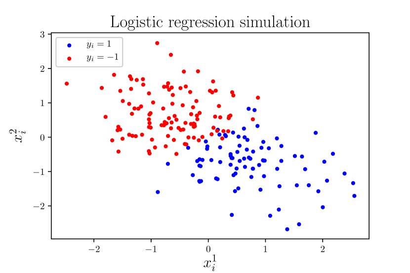
(a) Dataset 1

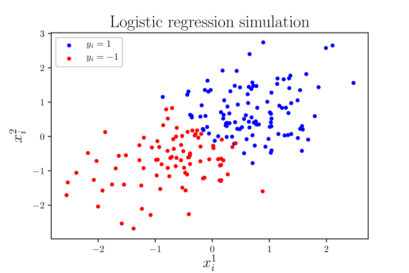
(b) Dataset 2

Figure S6: Data distribution for logistic regression to simulate non-i.i.d. data. Half of the device hold first dataset, and the other half the second one.

C.1.1 Least-square regression

In this section, we present all figures generated using Least-Square regression. Figure S7 corresponds to Figure 1(a).

As explained in the main of the paper, in the case of $\sigma_{*}\neq 0$ (Figure S7), algorithm using memory (i.e Diana and Artemis) are not expected to outperform those without (i.e QSQGD and Bi-QSGD). On the contrary, they saturate at a higher level. However, as soon as the noise at the optimum is $0$ (Figure S8), all algorithms (regardless of memory), converge at a linear rate exactly as classical SGD.

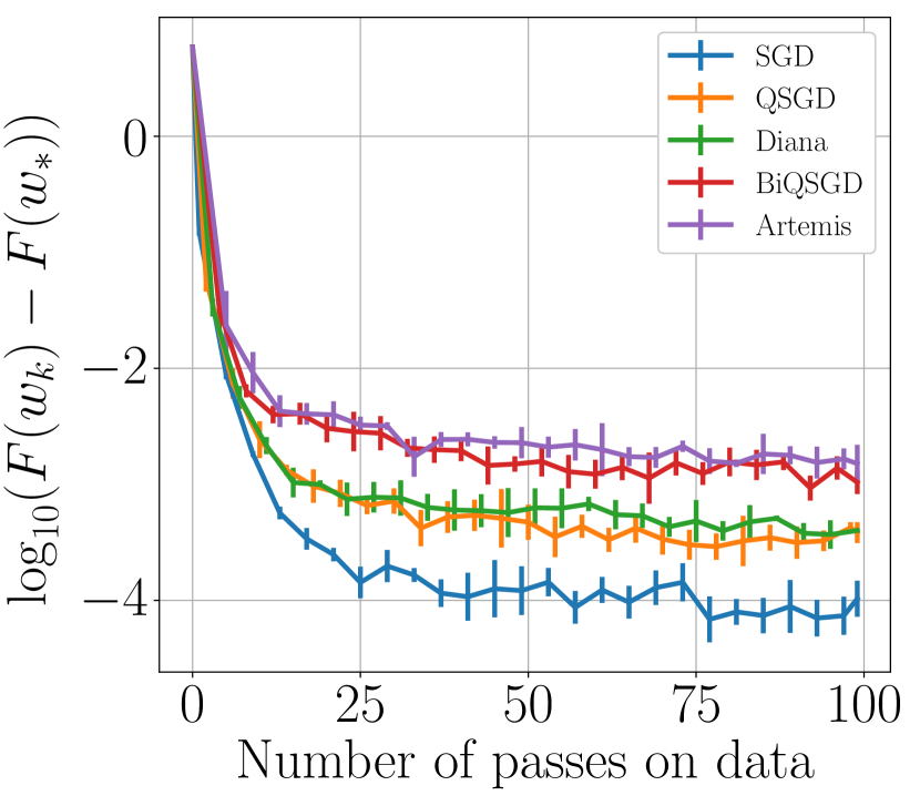
(a) LSR: $\sigma_{*}^{2}\neq 0$

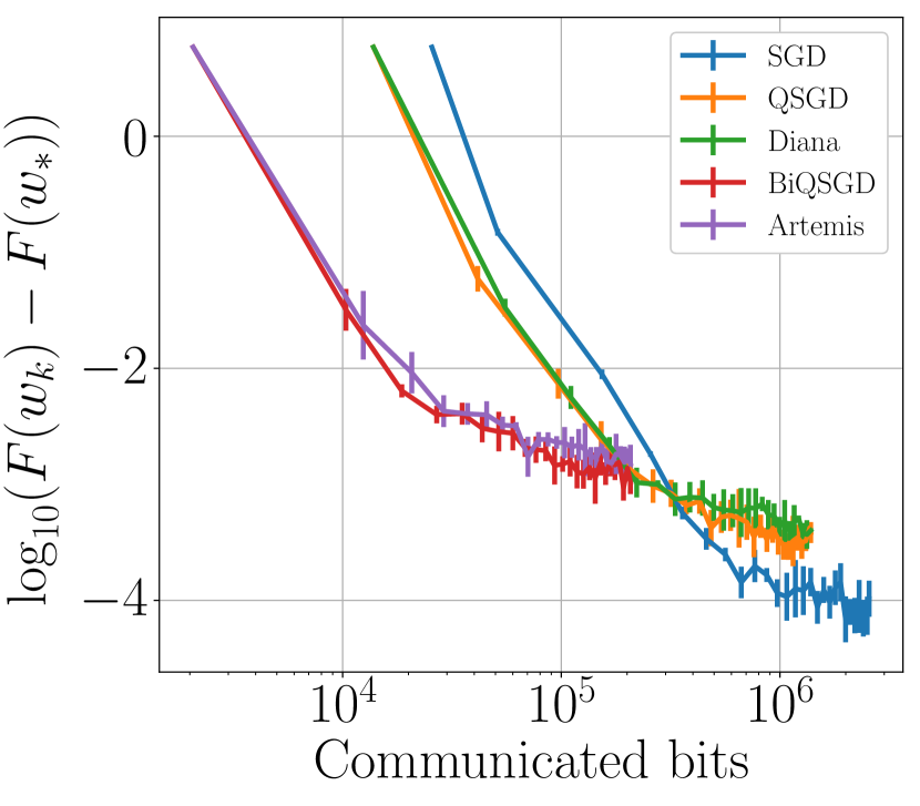
(b) X-axis in # bits.

Figure S7: Synthetic dataset, Least-Square Regression with noise ($\sigma_{*}\neq 0$). In a situation where data is i.i.d., the memory does not present much interest, and has no impact on the convergence. Because $\sigma_{*}^{2}\neq 0$, all algorithms saturate ; and saturation level is higher for double compression (Artemis, Bi-QSGD), than for simple compression (Diana, QSGD) or than for SGD. This corroborates findings in Theorem 1 and Theorem 3.

(a) LSR: $\sigma_{*}^{2}=0$

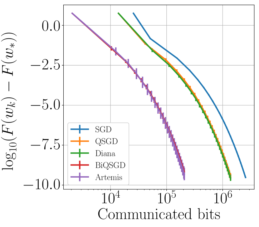
(b) X-axis in # bits.

Figure S8: Synthetic dataset, Least-Square Regression without noise ($\sigma_{*}=0$). Without surprise, with i.i.d data and $\sigma_{*}=0$, the convergence of each algorithm is linear. Thus, in i.i.d. settings, the impact of the memory is negligible, but this will not be the case in the non-i.i.d. settings as underlined by Figure S9.

C.1.2 Logistic regression

In this section, we present all figures generated using a logistic regression model. Figure S9 corresponds to Figure 1(b). Data is non-i.d.d. and we use a full batch gradient descent to get $\sigma_{*}=0$ to shed into light the impact of memory over convergence.

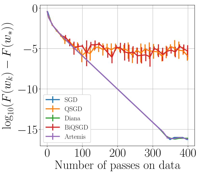
(a) LR: $\sigma_{*}^{2}=0$

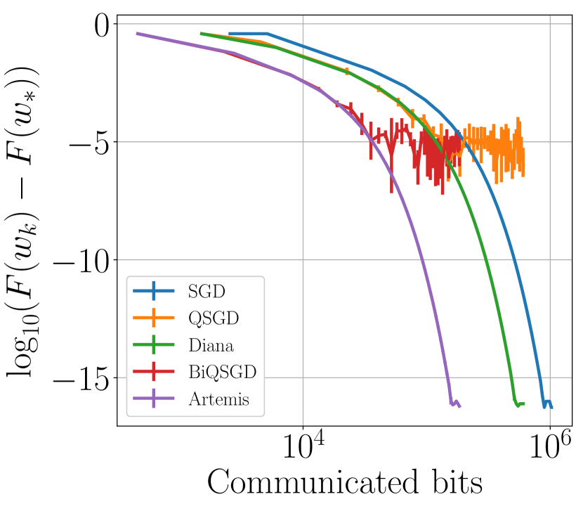
(b) X-axis in # bits.

Figure S9: Synthetic dataset, Logistic Regression on non-i.i.d. data using a batch gradient descent (to get $\sigma_{*}=0$). The benefit of memory is obvious, it makes the algorithm to converge linearly, while algorithms without are saturating at a high level. This stress on the importance of using the memory in non-i.i.d. settings.

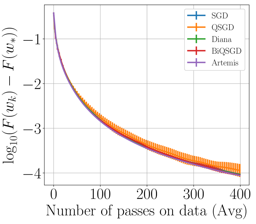
(a) LR: $\sigma_{*}^{2}=0$

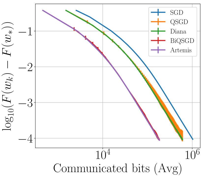
(b) X-axis in # bits.

Figure S10: Polyak-Ruppert averaging, synthetic dataset. Logistic Regression on non-i.i.d. data using a batch gradient descent (to get $\sigma_{*}=0$) and a Polyak-Ruppert averaging. The convergence is linear as predicted by Theorem 2 because $\sigma_{*}=0$. Best seen in colors.

Figure S10 is using same data and configuration as Figure S9, except that it is combined with a Polyak-Ruppert averaging. Note that in the absence of memory the variance increases compared to algorithms using memory. To generate these figures, we didn’t take the optimal step size. But if we took it, the trade-off between variance and bias would be worse and algorithms using memory would outperform those without.

C.2 Real datasets: Quantum and Superconduct

In this section, we present details about experiments conducted on real-life datasets: superconduct (from Caruana et al. [2004]) where we use a least-square regression, and quantum (from Hamidieh [2018]) with a logistic regression. All figures can be found in the notebooks provided in supplementary materials.

In this following, we present results on superconduct and quantum in the setting of full device participation. We detail experiments in the PP setting in Subsection C.2.1. Next, we address the issue of the optimal step size in Subsection C.2.2. In Subsection C.2.3 we compare Artemis to other existing algorithm doing compression in a distributed learning framework. Finally, we estimate in Subsection C.3 the carbon footprint of our work.

In order to simulate non-i.i.d. data and to make the experiments closer to real-life usage, we split the dataset in heterogeneous groups using a Gaussian mixture clustering on TSNE representations (defined by Maaten & Hinton [2008]). Thus, the data are highly non-i.i.d. and unbalanced over devices. We plot on Figure S11 the TSNE representation of the two real datasets.

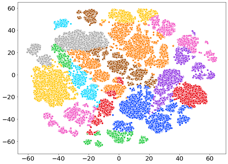
(a) Quantum dataset: $20$ clusters. Each cluster has between $900$ and $10500$ points with a median at $2300$ points.

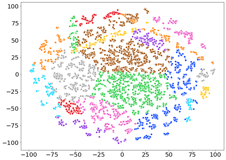
(b) Superconduct dataset: $20$ cluster. Each cluster has between $250$ and $3900$ points with a median at $750$ points.

Figure S11: TSNE representations. Best seen in colors.

There are $N=20$ devices for superconduct and quantum datasets. For superconduct, there are between $250$ and $3900$ points by worker, with a median at $750$ ; and for quantum, there are between $900$ and $10500$ points, with a median at $2300$. On each figure, we indicate which step size $\gamma$ has been used.

Convex settings are given in Table S1. Experiments have been performed with $150$ epochs in the stochastic regime, and $800$ epochs in the full batch regime. We use quantization [defined in Alistarh et al., 2017] with $s=2^{0}$ for all experiments, except in the case of partial participation where we used $s=2^{1}$.

Table S1: Settings of experiments.

Settings	quantum	superconduct
references	Caruana et al. [2004]	Hamidieh [2018]
model	LR	LSR
dimension $d$	$66$	$82$
training dataset size	$50,000$	$21,200$
batch size $b$	$256$	$64$
compression rate $s$	$2^{0}$ (i.e. two levels)
norm quantization	$\|\cdot\|_{2}$
momentum $m$	no momentum
step size $\gamma$	$1/L$

Figures S14 and S12 correspond to Figure 2. We observe on these figures the benefit of the memory. The level of saturation of algorithms using memory is much lower than those without memory. Additionally, Theorem 1 highlights that the level of saturation (see constant $E$ of Table 2) is proportional to the level of compression $\omega_{\mathcal{C}}^{\mathrm{up}/\mathrm{dwn}}$. This is indeed observed on Figures S14, S12, S15 and S13.

In the case of the quantum dataset (see Figure S12), Artemis is not only better than Bi-QSGD, but in fact, as good as QSGD. That is to say, we achieve to make an algorithm using a bidirectional compression, as good as an algorithm handling unidirectional compression.

On Figures S13 and S15, we represent the convergence of the five algorithms in a full batch mode resulting to $\sigma_{*}=0$. In this case, as the dependency on $B^{2}$ is removed, Theorem 1 predicts that we must have a linear convergence for algorithms using memory. This is experimentally observed.

Memory trade-off: batch size, noise at the optimum, and heterogeneity. Because the variance of the algorithm (see constant $E$ of Table 2) is divided by the batch size $b$, the choice of this hyperparameter is not without importance. Indeed, reducing the batch size will increase the impact of $\sigma_{*}$ on the convergence’s rate, while the impact of $B^{2}$ will remain constant. Thus, there is a trade-off: if the batch-size is too small, the quantity $\sigma_{*}/b$ will become larger than $B^{2}$, and the impact of the memory will be hidden by the second term depending on the dataset heterogeneity. This will lead Artemis-like algorithms to fail: the memory term is canceled by the high heterogeneity. On the other hand, if the dataset does not present enough heterogeneity, the constant $B^{2}$, will be negligible making memory useless, or even penalizing.

To summarize, Figures S14, S12, S15 and S13 underline the benefit of using memory in the stochastic and full batch regime for non-i.i.d. datasets.

(a) X-axis in # epoch

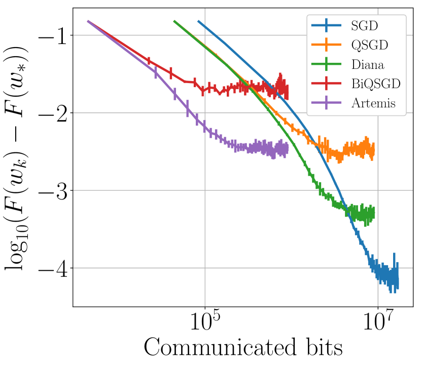
(b) X-axis in # bit

Figure S12: Quantum. least-square regression, $\sigma_{*}\neq 0$, $\gamma=1/L$, $b=256$, non-i.i.d.. Best seen in colors.

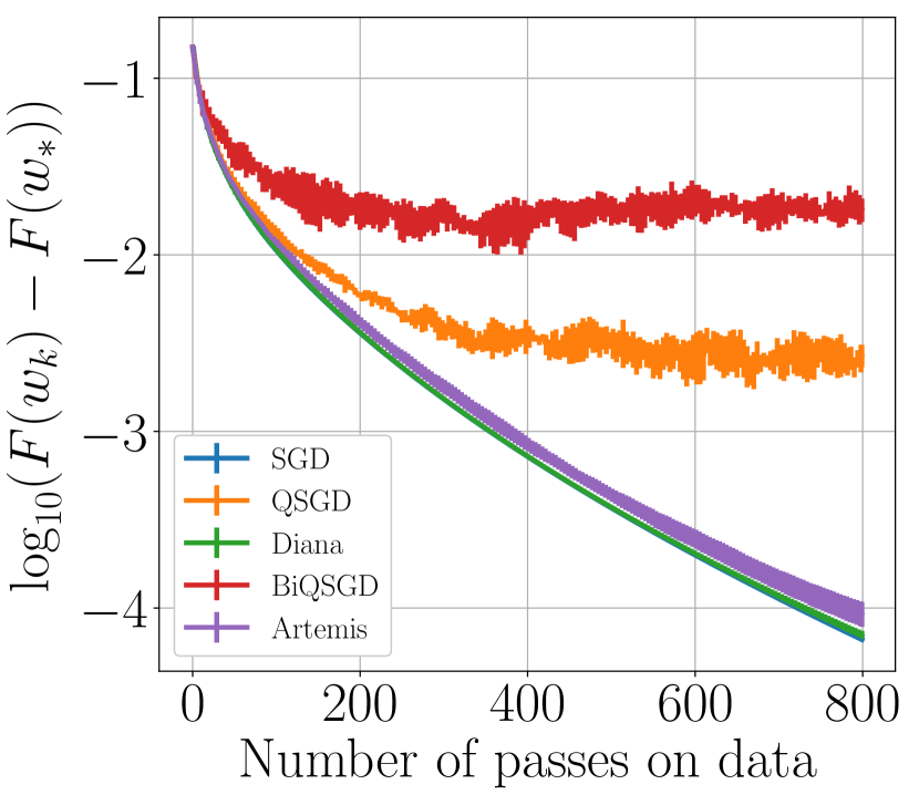
(a) X-axis in # epoch

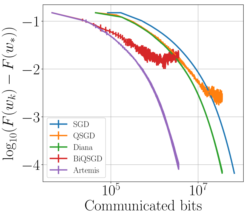
(b) X-axis in # bit

Figure S13: Quantum. least-square regression, $\sigma_{*}=0$, $\gamma=1/L$, $b=256$, non-i.i.d.. Best seen in colors.

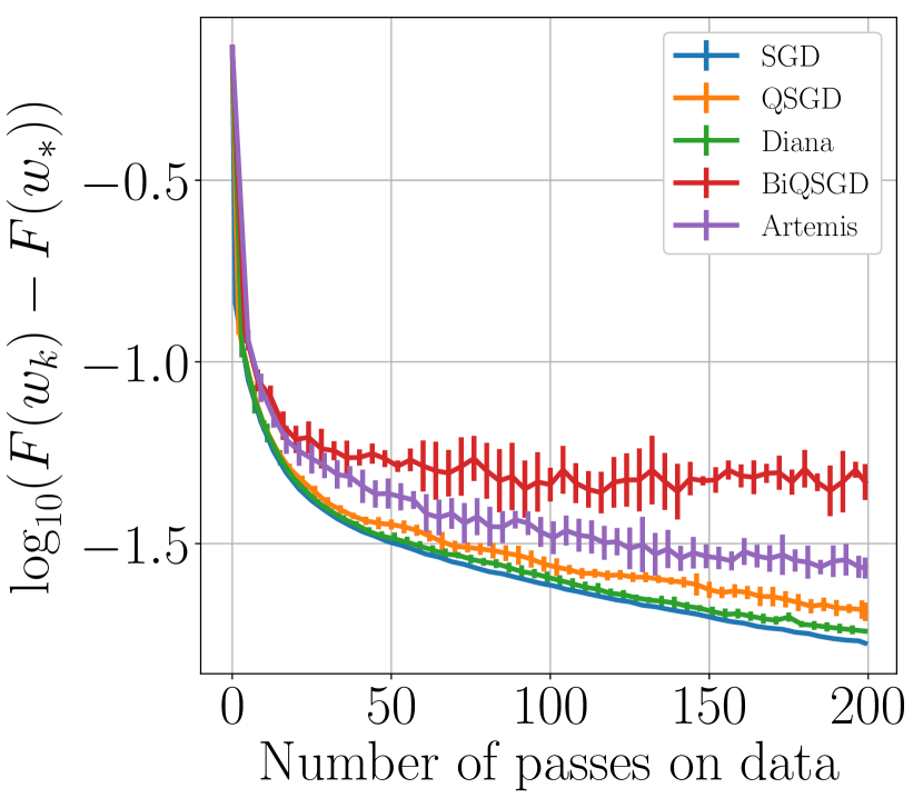
(a) X-axis in # epochs

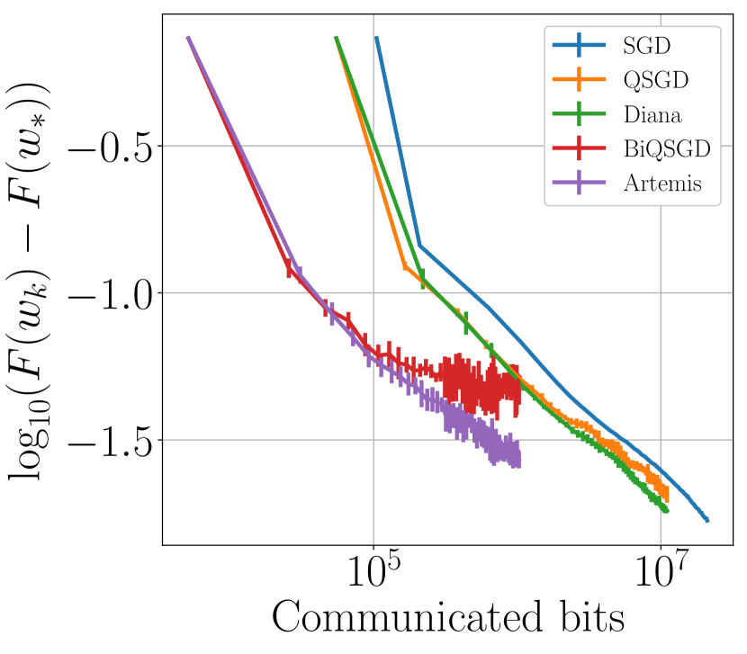
(b) X-axis in # bit

Figure S14: Superconduct. least-square regression, $\sigma_{*}\neq 0$, $\gamma=1/L$, $b=64$, non-i.i.d.. Best seen in colors.

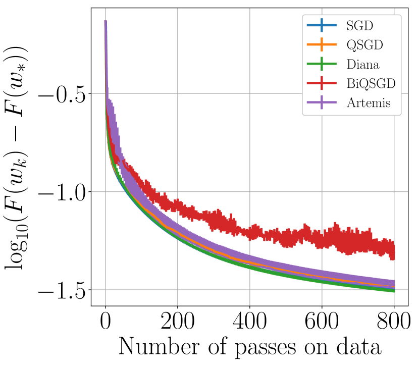
(a) X-axis in # epochs

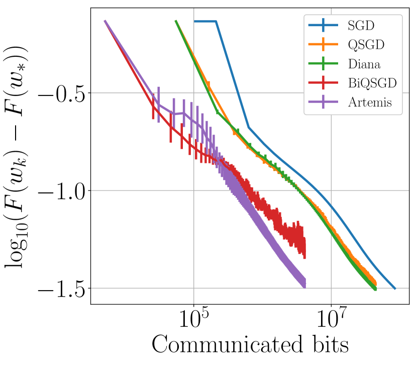
(b) X-axis in # bit

Figure S15: Superconduct. least-square regression, $\sigma_{*}=0$, $\gamma=1/L$, $b=64$, non-i.i.d.. Best seen in colors.

C.2.1 Partial participation

In this section we provide additional experiments on partial participation in the stochastic regime. Only half of the devices (randomly sampled) participate at each round, we use $2^{1}$-quantization.

Figure S16 presents the first naive approach (PP1) to handle partial participation. This naive solution fails to properly converge. In the other hand, algorithms using PP2 - SGD with memory i.e Artemis with $\omega_{\mathcal{C}}^{\mathrm{up}/\mathrm{dwn}}=0$, Artemis with unidirectional compression i.e. $\omega_{\mathcal{C}}^{\mathrm{dwn}}=0$ and Artemis with $\omega_{\mathcal{C}}^{\mathrm{up}/\mathrm{dwn}}\neq 0$ - presents much better convergence, see Figure S17. As an example, SGD with memory matches the results of SGD in the case of full participation (Figures S14 and S12). However, the convergence of QSGD and Bi-QSGD is unchanged as there is no difference between the two approaches in the absence of memory.

The result in the full gradient regime is given in Section 5. On Figures 4 and 3, we can observe that our new algorithm PP2 has a linear convergence unlike PP1.

As a conclusion on partial participation: with PP2, we observe the significant impact of memory when using non-i.i.d. data. Comparing Figure S17 to Figure S16, the saturation of algorithms with $\alpha$ different to zero (i.e. using memory) is much lower; and classical SGD is outperformed by its variant using the memory mechanism.

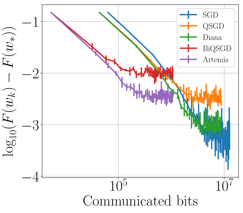
(a) Quantum

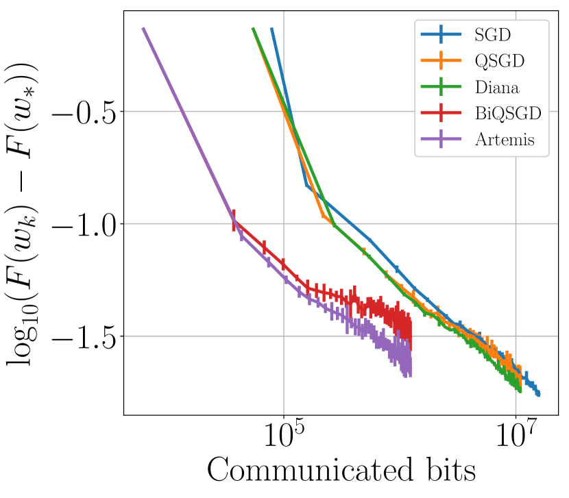
(b) Superconduct

Figure S16: Partial participation, stochastic regime - PP1. $\sigma_{*}\neq 0$, $N=20$ workers, $p=0.5$, $b>1$ ($150$ iter.) With this variant, all algorithms are saturating at a high level.

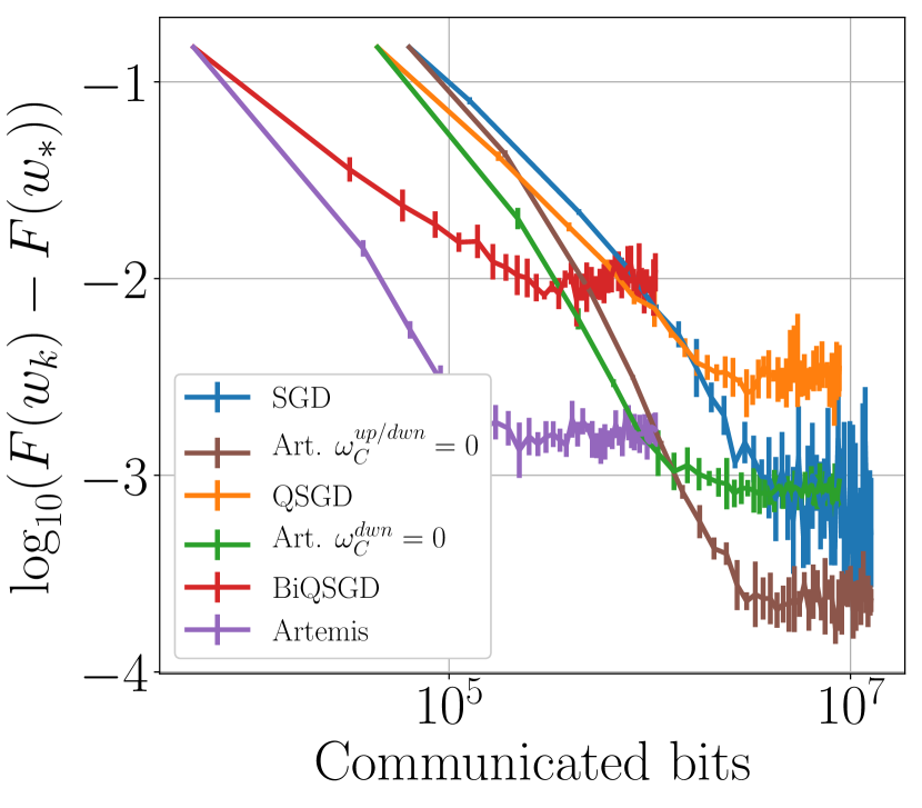
(a) Qauntum

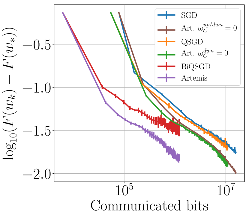
(b) Superconduct

Figure S17: Partial participation, stochastic regime - PP2. $\sigma_{*}\neq 0$, $N=20$ workers, $p=0.5$, $b>1$ ($150$ iter.).

C.2.2 Optimized step size

In this section, we want to address the issue of the optimal step size. On Figure S18 we plot the minimal loss after $150$ iterations for each of the $5$ algorithms. We can see that algorithms with memory clearly outperform those without. Then, on Figure S19 we present the loss of Artemis after $150$ iterations for various step size: $\frac{N=20}{2L}$, $\frac{5}{L}$, $\frac{2}{L}$, $\frac{1}{L}$, $\frac{1}{2L}$, $\frac{1}{4L}$, $\frac{1}{8L}$ and $\frac{1}{16L}$. This helps to understand which step size should be taken to obtain the best accuracy after $k$ in $\llbracket 1,150\rrbracket$ iterations. Finally, on Figure S20, we plot the loss obtained with the optimal step size $\gamma_{opt}$ of each algorithms (found with Figure S18) w.r.t the number of communicated bits.

On Figure S18, it is interesting to note that the memory allows to increase the maximal step size. So, the optimal step size is $\gamma_{opt}=\frac{1}{L}$ for Artemis , but is $\gamma_{opt}=\frac{1}{2L}$ for BiQSGD.

We plot the loss of Artemis after $150$ iterations for different step size on Figure S19. As stressed by Figure S18, after $150$ iterations, the best accuracy for both datasets is indeed obtained with $\gamma_{opt}=\frac{1}{L}$. And we observe that (as for Vanilla SGD), the optimal step size of Artemis decreases with the number of iterations (e.g., for quantum, it is $1/L$ before 50 iterations and $1/2L$ after). This is consistent with Theorem 1.

Figure S20 plots the loss of each algorithm obtained with its optimal step size $\gamma$ i.e. the step size that attains the lowest error after $150$ iterations. For instance $\gamma=\frac{1}{L}$ for Artemis, but $\gamma=\frac{2}{L}$ for SGD. For both superconduct and quantum datasets, taking the optimal step size leads Artemis to superior performance than other variants w.r.t. both accuracy and number of bits.

In conclusion of this subsection, Figures S19, S18 and S20 allow to conclude on the significant impact of memory in a non-i.i.d. settings, and to claim that bidirectional compression with memory is by far superior (up to a threshold) to the four other algorithm: SGD, QSGD, Diana and BiQSGD.

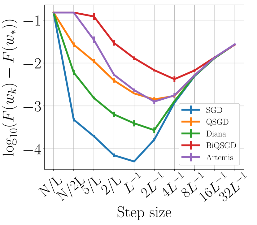
(a) Quantum

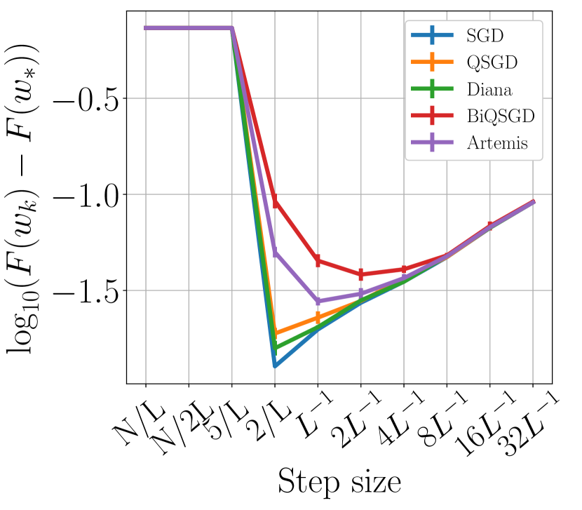
(b) Superconduct

Figure S18: Searching for the optimal step size $\gamma_{opt}$ for each algorithm. X-axis - value on step size, Y-axis - minimal loss after running $250$ iterations

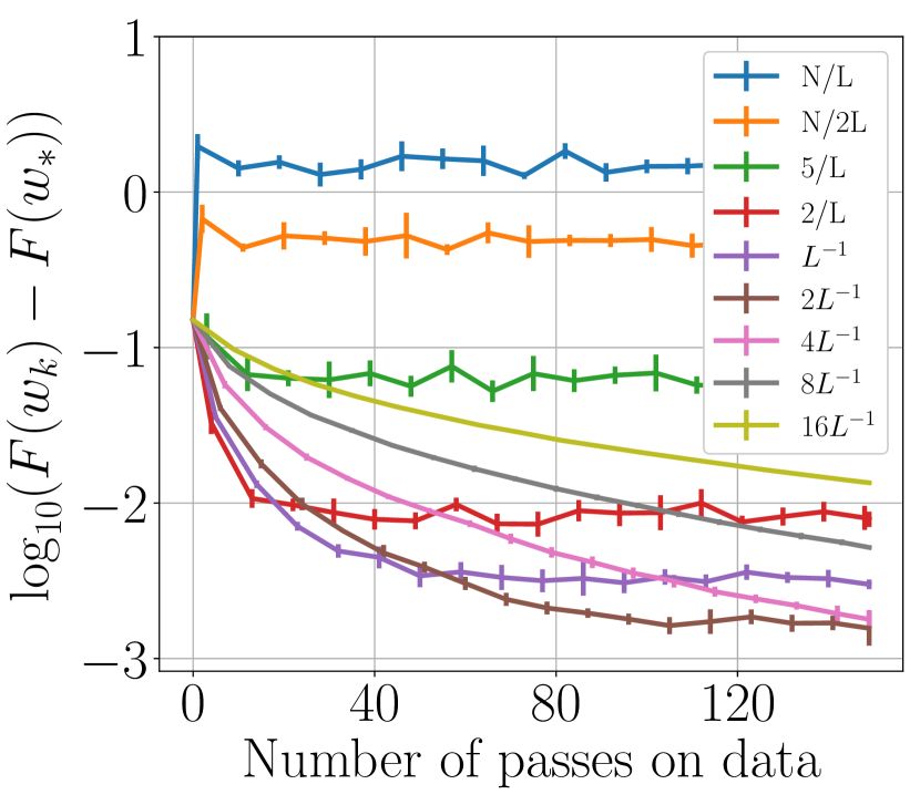
(a) Quantum

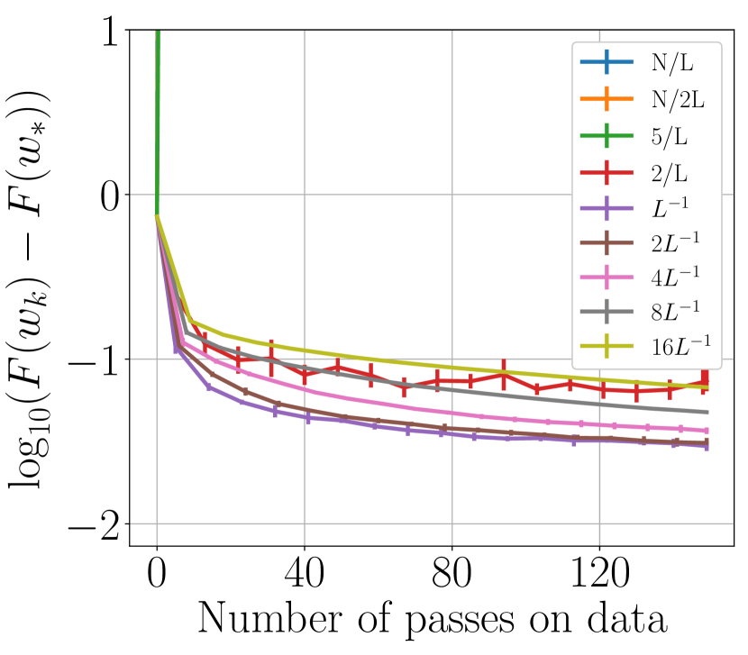
(b) Superconduct

Figure S19: Loss w.r.t. step size $\gamma$.

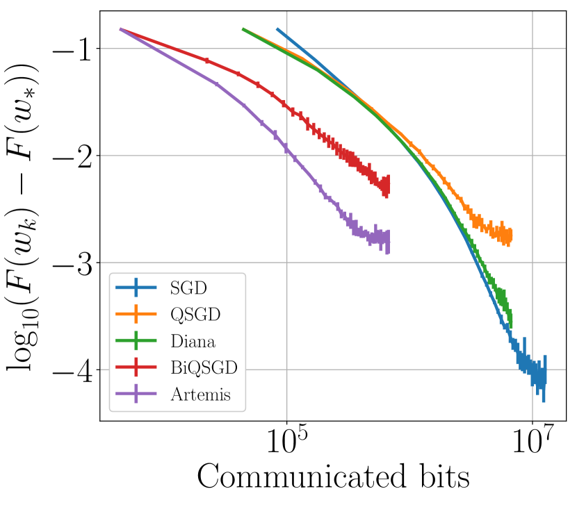
(a) Quantum

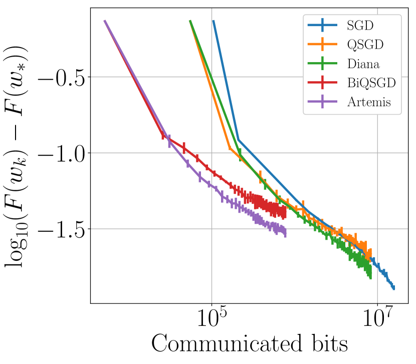
(b) Superconduct

Figure S20: Optimal step size for each of the algorithms. X-axis in # bits.

C.2.3 Comparing Artemis with other existing algorithms

On Figure S21 we compare Artemis with other existing algorithms: FedSGD, FedPAQ, Diana, Dore and Double-Squeeze. We take $\gamma=1/(2L)$ because otherwise FedSGD and FedPAQ diverge. These two algorithms present worse performance because they have not been designed for non-i.i.d. datasets.

We can observe that Double-Squeeze (which only uses error-feedback) is outperformed by Artemis. Besides, we observe that Dore (which combines this mechanism with memory) has identical rate of convergence than Artemis. It underlines that for unbiased operators of compression, the enhancement comes from the memory and not from the error-feedback.

FedPAQ (unidirectional compression) has a very fast convergence during first iterations, but then saturates at a level higher than for Artemis-like algorithms. FedSGD (no compression) presents a convergence’s rate worse that vanilla SGD because it does not correctly handle heterogeneous datasets.

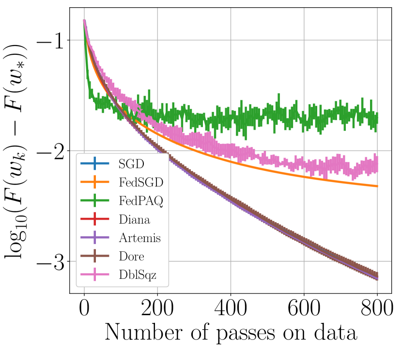
(a) Superconduct

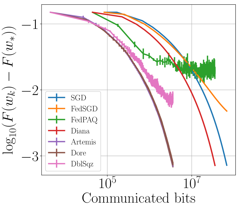
(b) Superconduct

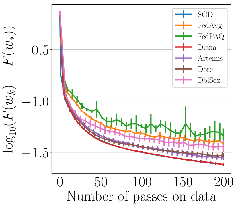
(c) Quantum

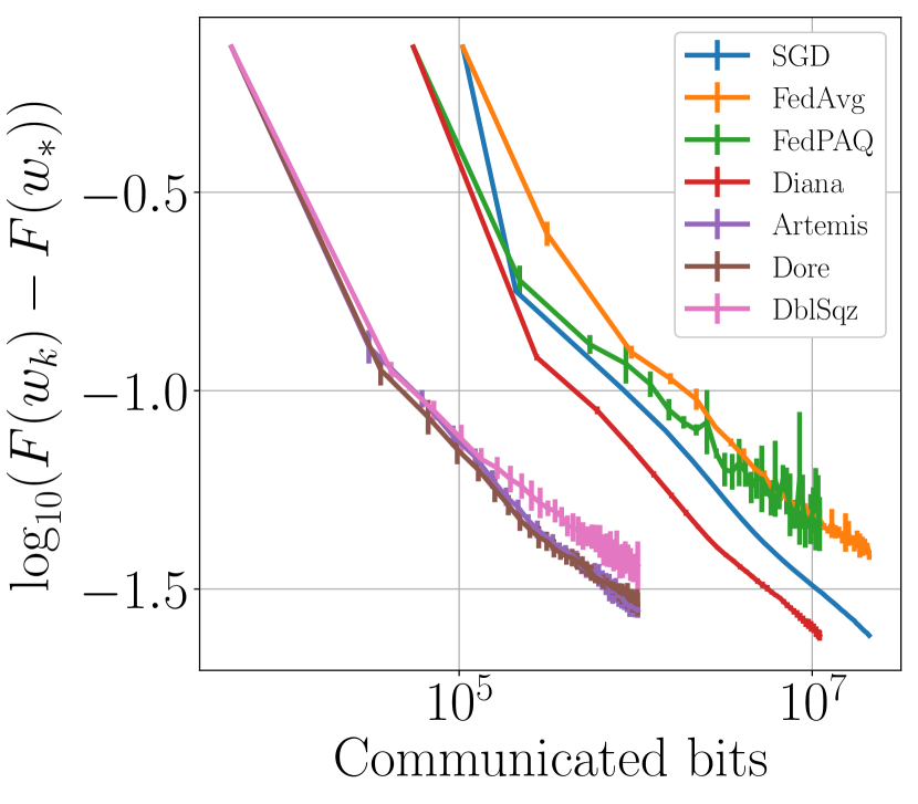
(d) Quantum

Figure S21: Artemis compared to other existing algorithms. $\gamma=1/(2L)$, X-axis in # epoch or in # bits.

C.3 CPU usage and Carbon footprint

As part as a community effort to report the amount of experiments that were performed, we estimated that overall our experiments ran for 220 to 270 hours end to end. We used an Intel(R) Xeon(R) CPU E5-2667 processor with 16 cores.

The carbon emissions caused by this work were subsequently evaluated with Green Algorithm built by Lannelongue et al. [2020]. It estimates our computations to generate $30$ to $35$ kg of CO2, requiring $100$ to $125$ kWh. To compare, it corresponds to about $160$ to $200$km by car. This is a relatively moderate impact, matching the goal to keep the experiments for an illustrative purpose.

Appendix D Technical Results

In this section, we introduce a few technical lemmas that will be used in the proofs. In Subsection D.1, we give four simple lemmas, while in Subsection D.2 we present a lemma which will be invoked in Appendix E to demonstrate Theorems S5, S6 and S7.

Notation.

Let $k^{*}\in\mathbb{N}$ and $(a_{k+1}^{i})_{i=0}^{N}\in(\mathbb{R}^{d})^{N}$ random variables independent of each other and $\mathcal{J}_{k+1}$-measurable, for a $\sigma$-field $\mathcal{J}_{k+1}$ s.t. $(B_{k}^{i})^{N}_{i=1}$ are independent of $\mathcal{J}_{k+1}$.. Then in all the following demonstration, we note $a_{k+1}=\frac{1}{N}\sum_{i=1}^{N}a_{k+1}^{i}$ and $a_{k+1,S_{k}}=\frac{1}{pN}\sum_{i\in S_{k}}a_{k+1}^{i}$.

The vector $a_{k+1}$ (resp. the $\sigma$-field $\mathcal{J}_{k+1}$) may represent various objects, for instance : $g_{k+1}$, $\widehat{g}_{k+1}$, $G_{k+1}$ (resp. $\mathcal{F}_{k+1}$, $\mathcal{G}_{k+1}$, $\mathcal{H}_{k+1}$).

Remark 4.

We can add the following remarks on the assumptions.

• Assumption 6 can be extended to probabilities depending on the worker $(p_{i})_{i\in\llbracket 1,N\rrbracket}$.

• Assumption 5 requires in fact to access a sequence of i.i.d. compression operators $\mathcal{C}_{\mathrm{up}/\mathrm{dwn},k}$ for $k\in\mathbb{N}$ – but for simplicity, we generally omit the $k$ index.

• Assumption 4 in fact only requires that for any $i\in\llbracket 1,N\rrbracket$, $\mathbb{E}\left[\|g_{k+1,*}^{i}-\nabla F_{i}(w_{*})\|^{2}\leavevmode\nobreak\ \middle|\leavevmode\nobreak\ \mathcal{H}_{k}\right]\leq\frac{(\sigma_{*})_{i}^{2}}{b}$, and the results then hold for $\sigma_{*}=\frac{1}{N}\sum_{i=1}^{N}(\sigma_{*})_{i}^{2}$. In other words, the bounds does not need to be uniform over workers, only the average truly matters.

D.1 Useful identities and inequalities

Lemma S1.

Let $N\in\mathbb{N}$ and $d\in\mathbb{N}$. For any sequence of vector $(a_{i})_{i=1}^{N}\in\mathbb{R}^{d}$, we have the following inequalities:

$$\left\|\sum_{i=1}^{N}a_{i}\right\|^{2}\leq\left(\sum_{i=1}^{N}\left\|a_{i}\right\|\right)^{2}\leq N\sum_{i=1}^{N}\left\|a_{i}\right\|^{2}\,.$$

The first part of the inequality corresponds to the triangular inequality, while the second part is Cauchy’s inequality.

Lemma S2.

Let $\alpha\in[0,1]$ and $x,y\in(\mathbb{R}^{d})^{2}$, then:

$$\left\|\alpha x+(1-\alpha)y\right\|^{2}=\alpha\left\|x\right\|^{2}+(1-\alpha)\left\|y\right\|^{2}-\alpha(1-\alpha)\left\|x-y\right\|^{2}\,.$$

This is a norm’s decomposition of a convex combination.

Lemma S3.

Let $X$ be a random vector of $\mathbb{R}^{d}$, then for any vector $x\in\mathbb{R}^{d}$:

$$\mathbb{E}\left\|X-\mathbb{E}X\right\|^{2}=\mathbb{E}\left\|X-x\right\|^{2}-\left\|\mathbb{E}X-x\right\|^{2}\,.$$

This equality is a generalization of the well know decomposition of the variance (with $x=0$).

Lemma S4.

If $F:\mathcal{X}\subset\mathbb{R}^{d}\rightarrow\mathbb{R}$ is strongly convex, then the following inequality holds:

$$\forall(x,y)\in\mathbb{R}^{d},\left\langle\nabla F(x)-\nabla F(y)\leavevmode\nobreak\ \middle|\leavevmode\nobreak\ x-y\right\rangle\geq\mu\left\|x-y\right\|^{2}\,.$$

This inequality is a consequence of strong convexity and can be found in [Nesterov, 2004, equation $2.1.22$].

D.2 Lemmas for proof of convergence

Below are presented technical lemmas needed to prove the contraction of the Lyapunov function for Theorems S5 and S6. In this section we assume that Assumptions 6, 5, 1, 2, 3 and 4 are verified. In Subsections D.2.2 and D.2.1 we separate lemmas that required only for the case with memory or without.

The first lemma is very simple and straightforward from the definition of $\Delta_{k}^{i}$. We remind that $\Delta_{k}^{i}$ is the difference between the computed gradient and the memory hold on device $i$. It corresponds to the information which will be compressed and sent from device $i$ to the central server.

Lemma S5 (Bounding the compressed term).

The squared norm of the compressed term sent by each node to the central server can be bounded as following:

$$\forall k\in\mathbb{N}\,,\,\forall i\in\llbracket 1,N\rrbracket\,,\quad\left\|\Delta_{k}^{i}\right\|^{2}\leq 2\left(\left\|g_{k+1}^{i}-h_{*}^{i}\right\|^{2}+\left\|h_{k}^{i}-h_{*}^{i}\right\|^{2}\right)\,.$$

Proof.

Let $k\in\mathbb{N}$ and $i\in\llbracket 1,N\rrbracket$, we have by definition:

$$\left\|\Delta_{k}^{i}\right\|^{2}=\left\|g_{k+1}^{i}-h_{k}^{i}\right\|^{2}=\left\|(g_{k+1}^{i}-h_{*}^{i})+(h_{*}^{i}-h_{k}^{i})\right\|^{2}\,.$$

Applying Lemma S1 gives the expected result. ∎

Below, we show up a recursion over the memory term $h_{k}^{i}$ involving the stochastic gradients. This recursion will be used in Lemma S13. The existence of recursion has been first shed into light by Mishchenko et al. [2019].

Lemma S6 (Expectation of memory term).

The memory term $h_{k+1}^{i}$ can be expressed using a recursion involving the stochastic gradient $g_{k+1}^{i}$:

$$\forall k\in\mathbb{N}\,,\,\forall i\in\llbracket 1,N\rrbracket\,,\quad\mathbb{E}\left[h_{k+1}^{i}\leavevmode\nobreak\ \middle|\leavevmode\nobreak\ \mathcal{F}_{k+1}\right]=(1-\alpha)h_{k}^{i}+\alpha g_{k+1}^{i}\,.$$

Proof.

Let $k\in\mathbb{N}$ and $i\in\llbracket 1,N\rrbracket$. We just need to decompose $h^{i}_{k}$ using its definition:

$$h_{k+1}^{i}=h_{k}^{i}+\alpha\widehat{\Delta}_{k}^{i}=h_{k}^{i}+\alpha(\widehat{g}_{k+1}^{i}-h_{k}^{i})=(1-\alpha)h_{k}^{i}+\alpha\widehat{g}_{k+1}^{i}\,,$$

and considering that $\mathbb{E}\left[\widehat{g}_{k+1}^{i}\leavevmode\nobreak\ \middle|\leavevmode\nobreak\ \mathcal{F}_{k+1}\right]=g_{k+1}^{i}$ (Proposition S3), the proof is completed.

∎

In Lemma S7, we rewrite $\left\|g_{k+1}\right\|^{2}$ and $\left\|g_{k+1}-h_{*}^{i}\right\|^{2}$ to make appears:

1. the noise over stochasticity

2. $\left\|g_{k+1}-g_{k+1,*}\right\|^{2}$ which is the term on which will later be applied cocoercivity (see Assumption 2).

Lemma S7 is required to correctly apply cocoercivity in Lemma S14.

Lemma S7 (Before using co-coercivity).

Let $k\in\llbracket 0,K\rrbracket$ and $i\in\llbracket 1,N\rrbracket$. The noise in the stochastic gradients as defined in Assumptions 3 and 4 can be controlled as following:

$$\frac{1}{N}\sum_{i=1}^{N}\mathbb{E}\left[\left\|g_{k+1}^{i}\right\|^{2}\leavevmode\nobreak\ \middle|\leavevmode\nobreak\ \mathcal{H}_{k}\right]\leq\frac{2}{N}\sum_{i=1}^{N}\left(\mathbb{E}\left[\left\|g_{k+1}^{i}-g_{k+1,*}^{i}\right\|^{2}\leavevmode\nobreak\ \middle|\leavevmode\nobreak\ \mathcal{H}_{k}\right]+(\frac{\displaystyle\sigma_{*}^{2}}{\displaystyle b}+B^{2})\right)\,,$$ (S4)

$$\frac{1}{N}\sum_{i=1}^{N}\mathbb{E}\left[\left\|g_{k+1}^{i}-h_{*}^{i}\right\|^{2}\leavevmode\nobreak\ \middle|\leavevmode\nobreak\ \mathcal{H}_{k}\right]\leq\frac{2}{N}\sum_{i=1}^{N}\left(\mathbb{E}\left[\left\|g_{k+1}^{i}-g_{k+1,*}^{i}\right\|^{2}\leavevmode\nobreak\ \middle|\leavevmode\nobreak\ \mathcal{H}_{k}\right]+\frac{\displaystyle\sigma_{*}^{2}}{\displaystyle b}\right)\,.$$ (S5)

Proof.

Let $k\in\mathbb{N}$. For eq. S4:

$$\left\|g_{k+1}^{i}\right\|^{2} =\left\|g_{k+1}^{i}-g_{k+1,*}^{i}+g_{k+1,*}^{i}\right\|^{2}$$

$$\quad\leq 2\left(\left\|g_{k+1}^{i}-g_{k+1,*}^{i}\right\|^{2}+\left\|g_{k+1,*}^{i}\right\|^{2}\right)\text{using inequality of \lx@cref{creftypecap~refnum}{lem:two_inequalities}.}$$

Taking expectation with regards to filtration $\mathcal{H}_{k}$ and using Assumptions 3 and 4 gives the first result.

For eq. S5, we use Lemma S1 and we write:

$$\left\|g_{k+1}^{i}-h_{*}^{i}\right\|^{2} =\left\|\left(g_{k+1}^{i}-g_{k+1,*}^{i}\right)+\left(g_{k+1,*}^{i}-\nabla F_{i}(w_{*})\right)\right\|^{2}$$

$$\leq 2(\left\|g_{k+1}^{i}-g_{k+1,*}^{i}\right\|^{2}+\left\|g_{k+1,*}^{i}-\nabla F_{i}(w_{*})\right\|^{2})\,.$$

Taking expectation, we have:

$$\mathbb{E}\left[\left\|g_{k+1}^{i}-h_{*}^{i}\right\|^{2}\leavevmode\nobreak\ \middle|\leavevmode\nobreak\ \mathcal{H}_{k}\right] \leq 2\left(\mathbb{E}\left[\left\|g_{k+1}^{i}-g_{k+1,*}^{i}\right\|^{2}\leavevmode\nobreak\ \middle|\leavevmode\nobreak\ \mathcal{H}_{k}\right]+\mathbb{E}\left[\left\|g_{k+1,*}^{i}-\nabla F_{i}(w_{*})\right\|^{2}\leavevmode\nobreak\ \middle|\leavevmode\nobreak\ \mathcal{H}_{k}\right]\right)$$

$$\leq 2\left(\mathbb{E}\left[\left\|g_{k+1}^{i}-g_{k+1,*}^{i}\right\|^{2}\leavevmode\nobreak\ \middle|\leavevmode\nobreak\ \mathcal{H}_{k}\right]+\frac{\displaystyle\sigma_{*}^{2}}{\displaystyle b}\right)\text{\quad using \lx@cref{creftypecap~refnum}{asu:noise_sto_grad}.}$$

∎

Demonstrating that the Lyapunov function is a contraction requires to bound $\left\|g_{k+1,S_{k}}\right\|^{2}$ which needs to control each term $(\left\|g_{k+1,S_{k}}^{i}\right\|^{2})_{i=1}^{N}$ of the sum. This leads to invoke smoothness of $F$ (consequence of Assumption 2).

Lemma S8.

Regardless if we use memory, we have the following bound on the squared norm of the gradient, for all $k$ in $\mathbb{N}$:

$$\quad\mathbb{E}\left[\left\|g_{k+1,S_{k}}\right\|^{2}\leavevmode\nobreak\ \middle|\leavevmode\nobreak\ \mathcal{I}_{k}\right] \leq\frac{\displaystyle 1}{\displaystyle pN^{2}}\sum_{i=1}^{N}\mathbb{E}\left[\left\|g_{k+1}^{i}-h_{*}^{i}\right\|^{2}\leavevmode\nobreak\ \middle|\leavevmode\nobreak\ \mathcal{H}_{k}\right]+L\left\langle\nabla F(w_{k})\leavevmode\nobreak\ \middle|\leavevmode\nobreak\ w_{k}-w_{*}\right\rangle\,.$$

Proof.

Let $k\in\mathbb{N}$,

$$\left\|g_{k+1,S_{k}}\right\|^{2} =\left\|\frac{1}{pN}\sum_{i\in S_{k}}g_{k+1}^{i}\right\|^{2}$$

$$=\left\|\frac{1}{pN}\sum_{i\in S_{k}}\left(g_{k+1}^{i}-\nabla F_{i}(w_{k})\right)+\frac{1}{pN}\sum_{i\in S_{k}}\nabla F_{i}(w_{k})\right\|^{2}\,.$$

Now taking conditional expectation w.r.t $\sigma(\mathcal{I}_{k}\cup\mathcal{B}_{k})$ (including $\mathcal{B}_{k}$ in the $\sigma$-field allows to not consider the randomness associated to the device sampling):

$$\mathbb{E}\left[\left\|g_{k+1,S_{k}}\right\|^{2}\leavevmode\nobreak\ \middle|\leavevmode\nobreak\ \sigma(\mathcal{I}_{k}\cup\mathcal{B}_{k})\right] =\mathbb{E}\left[\left\|\frac{1}{pN}\sum_{i\in S_{k}}g_{k+1}^{i}-\nabla F_{i}(w_{k})+\frac{1}{pN}\sum_{i\in S_{k}}\nabla F_{i}(w_{k})\right\|^{2}\leavevmode\nobreak\ \middle|\leavevmode\nobreak\ \sigma(\mathcal{I}_{k}\cup\mathcal{B}_{k})\right]\,.$$

Expanding this squared norm:

$$\mathbb{E}\left[\left\|g_{k+1,S_{k}}\right\|^{2}\leavevmode\nobreak\ \middle|\leavevmode\nobreak\ \sigma(\mathcal{I}_{k}\cup\mathcal{B}_{k})\right] =\mathbb{E}\left[\left\|\frac{1}{pN}\sum_{i\in S_{k}}g_{k+1}^{i}-\nabla F_{i}(w_{k})\right\|^{2}\leavevmode\nobreak\ \middle|\leavevmode\nobreak\ \sigma(\mathcal{I}_{k}\cup\mathcal{B}_{k})\right]$$

$$\qquad+2\mathbb{E}\left[\left\langle\frac{1}{pN}\sum_{i\in S_{k}}g_{k+1}^{i}-\nabla F_{i}(w_{k})\leavevmode\nobreak\ \middle|\leavevmode\nobreak\ \frac{1}{pN}\sum_{i\in S_{k}}\nabla F_{j}(w_{k})\right\rangle\leavevmode\nobreak\ \middle|\leavevmode\nobreak\ \sigma(\mathcal{I}_{k}\cup\mathcal{B}_{k})\right]$$

$$\qquad+\mathbb{E}\left[\left\|\frac{1}{pN}\sum_{i\in S_{k}}\nabla F_{i}(w_{k})\right\|^{2}\leavevmode\nobreak\ \middle|\leavevmode\nobreak\ \sigma(\mathcal{I}_{k}\cup\mathcal{B}_{k})\right]\,.$$

Moreover, $\forall i,j\in\llbracket 1,N\rrbracket^{2},\mathbb{E}\left[\left\langle g_{k+1}^{i}-\nabla F_{i}(w_{k})\leavevmode\nobreak\ \middle|\leavevmode\nobreak\ \nabla F_{j}(w_{k})\right\rangle\leavevmode\nobreak\ \middle|\leavevmode\nobreak\ \sigma(\mathcal{I}_{k}\cup\mathcal{B}_{k})\right]=0$ and $\nabla F(w_{k})$ is $\sigma(\mathcal{I}_{k}\cup\mathcal{B}_{k})$-measurable:

$$\mathbb{E}\left[\left\|g_{k+1,S_{k}}\right\|^{2}\leavevmode\nobreak\ \middle|\leavevmode\nobreak\ \sigma(\mathcal{I}_{k}\cup\mathcal{B}_{k})\right] \leq\mathbb{E}\left[\left\|\frac{1}{pN}\sum_{i\in S_{k}}g_{k+1}^{i}-\nabla F_{i}(w_{k})\right\|^{2}\leavevmode\nobreak\ \middle|\leavevmode\nobreak\ \sigma(\mathcal{I}_{k}\cup\mathcal{B}_{k})\right]+\left\|\nabla F_{s_{k}}(w_{k})\right\|^{2}\,.$$ (S6)

To compute $\left\|\nabla F_{S_{k}}(w_{k})\right\|^{2}$, we apply cocoercivity (see Assumption 2) and next we take expectation w.r.t $\sigma$-algebra $\mathcal{I}_{k}$:

$$\mathbb{E}\left[\left\|\nabla F_{S_{k}}(w_{k})\right\|^{2}\leavevmode\nobreak\ \middle|\leavevmode\nobreak\ \mathcal{I}_{k}\right]=L\left\langle\mathbb{E}\left[\nabla F_{S_{k}}(w_{k})\leavevmode\nobreak\ \middle|\leavevmode\nobreak\ \mathcal{I}_{k}\right]\leavevmode\nobreak\ \middle|\leavevmode\nobreak\ w_{k}-w_{*}\right\rangle=L\left\langle\nabla F(w_{k})\leavevmode\nobreak\ \middle|\leavevmode\nobreak\ w_{k}-w_{*}\right\rangle$$

Now, for sake of clarity we note $\Pi=\left\|\frac{1}{pN}\sum_{i\in S_{k}}g_{k+1}^{i}-\nabla F_{i}(w_{k})\right\|^{2}$, then:

$$\mathbb{E}\left[\Pi\leavevmode\nobreak\ \middle|\leavevmode\nobreak\ \sigma(\mathcal{I}_{k}\cup\mathcal{B}_{k})\right] =\frac{1}{p^{2}N^{2}}\sum_{i\in S_{k}}\mathbb{E}\left[\left\|g_{k+1}^{i}-\nabla F_{i}(w_{k})\right\|^{2}\leavevmode\nobreak\ \middle|\leavevmode\nobreak\ \sigma(\mathcal{I}_{k}\cup\mathcal{B}_{k})\right]$$

$$\qquad+\frac{1}{p^{2}N^{2}}\sum_{i,j\in S_{k}/i\neq j}\underbrace{\mathbb{E}\left[\left\langle g_{k+1}^{i}-\nabla F_{i}(w_{k})\leavevmode\nobreak\ \middle|\leavevmode\nobreak\ g_{k+1}^{j}-\nabla F_{j}(w_{k})\right\rangle\leavevmode\nobreak\ \middle|\leavevmode\nobreak\ \sigma(\mathcal{I}_{k}\cup\mathcal{B}_{k})\right]}_{=0\text{ by independence of }(g_{k+1}^{i})_{i=0}^{N}}$$

$$=\frac{1}{p^{2}N^{2}}\sum_{i\in S_{k}}\mathbb{E}\left[\left\|(g_{k+1}^{i}-\nabla F_{i}(w_{*}))+(\nabla F_{i}(w_{*})-\nabla F_{i}(w_{k}))\right\|^{2}\leavevmode\nobreak\ \middle|\leavevmode\nobreak\ \sigma(\mathcal{I}_{k}\cup\mathcal{B}_{k})\right]\,.$$

Developing the squared norm a second time:

$$\mathbb{E}\left[\Pi\leavevmode\nobreak\ \middle|\leavevmode\nobreak\ \sigma(\mathcal{I}_{k}\cup\mathcal{B}_{k})\right] =\frac{1}{p^{2}N^{2}}\sum_{i\in S_{k}}\mathbb{E}\left[\left\|g_{k+1}^{i}-\nabla F_{i}(w_{*})\right\|^{2}\leavevmode\nobreak\ \middle|\leavevmode\nobreak\ \sigma(\mathcal{I}_{k}\cup\mathcal{B}_{k})\right]$$

$$\qquad+\frac{2}{p^{2}N^{2}}\sum_{i\in S_{k}}\mathbb{E}\left[\left\langle g_{k+1}^{i}-\nabla F_{i}(w_{*})\leavevmode\nobreak\ \middle|\leavevmode\nobreak\ \nabla F_{i}(w_{*})-\nabla F_{i}(w_{k})\right\rangle\leavevmode\nobreak\ \middle|\leavevmode\nobreak\ \sigma(\mathcal{I}_{k}\cup\mathcal{B}_{k})\right]$$

$$\qquad+\frac{1}{p^{2}N^{2}}\sum_{i\in S_{k}}\left\|\nabla F_{i}(w_{k})-\nabla F_{i}(w_{*}),\right\|^{2}$$

Then,

$$\mathbb{E}\left[\Pi\leavevmode\nobreak\ \middle|\leavevmode\nobreak\ \sigma(\mathcal{I}_{k}\cup\mathcal{B}_{k})\right] =\frac{1}{p^{2}N^{2}}\sum_{i\in S_{k}}\mathbb{E}\left[\left\|g_{k+1}^{i}-\nabla F_{i}(w_{*})\right\|^{2}\leavevmode\nobreak\ \middle|\leavevmode\nobreak\ \sigma(\mathcal{I}_{k}\cup\mathcal{B}_{k})\right]$$

$$\qquad-\frac{2}{p^{2}N^{2}}\sum_{i\in S_{k}}\left\langle\nabla F_{i}(w_{k})-\nabla F_{i}(w_{*})\leavevmode\nobreak\ \middle|\leavevmode\nobreak\ \nabla F_{i}(w_{k})-\nabla F_{i}(w_{*})\right\rangle$$

$$\qquad+\frac{1}{p^{2}N^{2}}\sum_{i\in S_{k}}\left\|\nabla F_{i}(w_{k})-\nabla F_{i}(w_{*})\right\|^{2}$$

$$=\frac{1}{p^{2}N^{2}}\sum_{i\in S_{k}}\mathbb{E}\left[\left\|g_{k+1}^{i}-\nabla F_{i}(w_{*})\right\|^{2}\leavevmode\nobreak\ \middle|\leavevmode\nobreak\ \sigma(\mathcal{I}_{k}\cup\mathcal{B}_{k})\right]-\left\|\nabla F_{i}(w_{k})-\nabla F_{i}(w_{*})\right\|^{2}\,$$

applying cocoercivity (Assumption 2):

$$\mathbb{E}\left[\Pi\leavevmode\nobreak\ \middle|\leavevmode\nobreak\ \sigma(\mathcal{I}_{k}\cup\mathcal{B}_{k})\right] \leq\frac{1}{p^{2}N^{2}}\sum_{i\in S_{k}}\mathbb{E}\left[\left\|g_{k+1}^{i}-\nabla F_{i}(w_{*})\right\|^{2}\leavevmode\nobreak\ \middle|\leavevmode\nobreak\ \sigma(\mathcal{I}_{k}\cup\mathcal{B}_{k})\right]-L\left\langle\nabla F_{i}(w_{k})-\nabla F_{i}(w_{*})\leavevmode\nobreak\ \middle|\leavevmode\nobreak\ w_{k}-w_{*}\right\rangle\,.$$ (S7)

Now we consider the randomness associated to device sampling. Remember that because $\mathcal{I}_{k}\subset\sigma(\mathcal{I}_{k}\cup\mathcal{B}_{k})$, we have $\mathbb{E}\left[\Pi\leavevmode\nobreak\ \middle|\leavevmode\nobreak\ \mathcal{I}_{k}\right]=\mathbb{E}\left[\mathbb{E}\left[\Pi\leavevmode\nobreak\ \middle|\leavevmode\nobreak\ \sigma(\mathcal{I}_{k}\cup\mathcal{B}_{k})\right]\leavevmode\nobreak\ \middle|\leavevmode\nobreak\ \mathcal{I}_{k}\right]$. Thus, we consider now $\Pi$ w.r.t. the $\sigma$-field $\mathcal{I}_{k}$

Handling first term of eq. S7:

$$\frac{1}{p^{2}N^{2}}\sum_{i\in S_{k}}\mathbb{E}\left[\left\|g_{k+1}^{i}-\nabla F_{i}(w_{*})\right\|^{2}\leavevmode\nobreak\ \middle|\leavevmode\nobreak\ \mathcal{I}_{k}\right] =\frac{1}{p^{2}N^{2}}\sum_{i=1}^{N}B_{k}^{i}\mathbb{E}\left[\left\|g_{k+1}^{i}-\nabla F_{i}(w_{*})\right\|^{2}\leavevmode\nobreak\ \middle|\leavevmode\nobreak\ \mathcal{I}_{k}\right]$$

$$=\frac{1}{pN^{2}}\sum_{i=1}^{N}\mathbb{E}\left[\left\|g_{k+1}^{i}-\nabla F_{i}(w_{*})\right\|^{2}\leavevmode\nobreak\ \middle|\leavevmode\nobreak\ \mathcal{I}_{k}\right]\,.$$

Handling second term of eq. S7:

$$L\left\langle\frac{1}{p^{2}N^{2}}\sum_{i\in S_{k}}\nabla F_{i}(w_{k})-\nabla F_{i}(w_{*})\leavevmode\nobreak\ \middle|\leavevmode\nobreak\ w_{k}-w_{*}\right\rangle=L\left\langle\frac{1}{p^{2}N^{2}}\sum_{i=0}^{N}\left(\nabla F_{i}(w_{k})-\nabla F_{i}(w_{*})\right)B_{k}^{i}\leavevmode\nobreak\ \middle|\leavevmode\nobreak\ w_{k}-w_{*}\right\rangle\,.$$

Taking expectation w.r.t $\sigma$-algebra $\mathcal{I}_{k}$:

$$\mathbb{E}\left[L\left\langle\frac{1}{p^{2}N^{2}}\sum_{i\in S_{k}}\nabla F_{i}(w_{k})-\nabla F_{i}(w_{*})\leavevmode\nobreak\ \middle|\leavevmode\nobreak\ w_{k}-w_{*}\right\rangle\leavevmode\nobreak\ \middle|\leavevmode\nobreak\ \mathcal{I}_{k}\right]$$

$$\qquad=L\left\langle\frac{1}{pN^{2}}\sum_{i=0}^{N}\nabla F_{i}(w_{k})-\nabla F_{i}(w_{*})\leavevmode\nobreak\ \middle|\leavevmode\nobreak\ w_{k}-w_{*}\right\rangle$$

$$\qquad=\frac{L}{pN}\left\langle\nabla F(w_{k})-\nabla F_{i}(w_{*})\leavevmode\nobreak\ \middle|\leavevmode\nobreak\ w_{k}-w_{*}\right\rangle\,.$$

Injecting this in eq. S7:

$$\mathbb{E}\left[\Pi\leavevmode\nobreak\ \middle|\leavevmode\nobreak\ \mathcal{I}_{k}\right] \leq\frac{1}{pN^{2}}\sum_{i=1}^{N}\mathbb{E}\left[\left\|g_{k+1}^{i}-\nabla F_{i}(w_{*})\right\|^{2}\leavevmode\nobreak\ \middle|\leavevmode\nobreak\ \mathcal{I}_{k}\right]-\frac{L}{pN}\left\langle\nabla F(w_{k})\leavevmode\nobreak\ \middle|\leavevmode\nobreak\ w_{k}-w_{*}\right\rangle\,.$$

Recall that we note $h_{*}^{i}=\nabla F_{i}(w_{*})$, returning to eq. S6 and invoking again cocoercivity:

$$\mathbb{E}\left[\left\|g_{k+1}\right\|^{2}\leavevmode\nobreak\ \middle|\leavevmode\nobreak\ \mathcal{I}_{k}\right] \leq\frac{1}{pN^{2}}\sum_{i=1}^{N}\mathbb{E}\left[\left\|g_{k+1}^{i}-h_{*}^{i}\right\|^{2}\leavevmode\nobreak\ \middle|\leavevmode\nobreak\ \mathcal{I}_{k}\right]+(1-\frac{1}{pN})L\left\langle\nabla F(w_{k})\leavevmode\nobreak\ \middle|\leavevmode\nobreak\ w_{k}-w_{*}\right\rangle\,,$$

which we simplify by considering that:

$$\mathbb{E}\left[\left\|g_{k+1}\right\|^{2}\leavevmode\nobreak\ \middle|\leavevmode\nobreak\ \mathcal{I}_{k}\right] \leq\frac{1}{pN^{2}}\sum_{i=1}^{N}\mathbb{E}\left[\left\|g_{k+1}^{i}-h_{*}^{i}\right\|^{2}\leavevmode\nobreak\ \middle|\leavevmode\nobreak\ \mathcal{I}_{k}\right]+L\left\langle\nabla F(w_{k})\leavevmode\nobreak\ \middle|\leavevmode\nobreak\ w_{k}-w_{*}\right\rangle\,.$$

∎

D.2.1 Lemmas for the case without memory

In this subsection, we give lemmas that are used only to demonstrate Theorem S5 (i.e. without memory).

Lemma S9 helps to pass for $k$ in $\mathbb{N}$ from $\widehat{g}_{k+1,S_{k}}$ to $(\widehat{g}_{k+1}^{i})_{i=1}^{N}$, this lemma will allow to invoke Lemma S10.

Lemma S9.

In the case without memory, we have the following bound on the squared norm of the compressed gradient (randomly sampled), for all $k$ in $\mathbb{N}$:

$$\mathbb{E}\left[\left\|\widehat{g}_{k+1,S_{k}}\right\|^{2}\leavevmode\nobreak\ \middle|\leavevmode\nobreak\ \mathcal{G}_{k+1}\right]=\frac{\displaystyle(1-p)}{\displaystyle pN^{2}}\sum_{i=0}^{N}\left\|\widehat{g}_{k+1}^{i}\right\|^{2}+\left\|\widehat{g}_{k+1}\right\|^{2}\,.$$

Proof.

The proof is quite straightforward using the expectation and the variance of $\widehat{g}_{k+1,S_{k}}$ computed in Propositions S7 and S8. We just need to decompose as following to easily obtain the result:

$$\mathbb{E}\left[\left\|\widehat{g}_{k+1,S_{k}}\right\|^{2}\leavevmode\nobreak\ \middle|\leavevmode\nobreak\ \mathcal{G}_{k+1}\right]=\mathbb{V}\left[\widehat{g}_{k+1,S_{k}}\leavevmode\nobreak\ \middle|\leavevmode\nobreak\ \mathcal{G}_{k+1}\right]+\left\|\mathbb{E}\left[\widehat{g}_{k+1,S_{k}}\leavevmode\nobreak\ \middle|\leavevmode\nobreak\ \mathcal{G}_{k+1}\right]\right\|^{2}$$

∎

Lemma S10 is used to remove the uplink compression noise straight after Lemma S9 has been applied.

Lemma S10 (Expectation of the squared norm of the compressed gradient when no memory).

In the case without memory, we have the following bound on the squared norm of the compressed gradient (randomly sampled), for all $k$ in $\mathbb{N}$:

$$\mathbb{E}\left[\left\|\widehat{g}_{k+1}\right\|^{2}\leavevmode\nobreak\ \middle|\leavevmode\nobreak\ \mathcal{H}_{k}\right]\leq\frac{\displaystyle\omega_{\mathcal{C}}^{\mathrm{up}}}{\displaystyle N^{2}}\sum_{i=0}^{N}\mathbb{E}\left[\left\|g_{k+1}^{i}\right\|^{2}\leavevmode\nobreak\ \middle|\leavevmode\nobreak\ \mathcal{H}_{k}\right]+\frac{\displaystyle 1}{\displaystyle N^{2}}\sum_{i=0}^{N}\mathbb{E}\left[\left\|g_{k+1}^{i}-h_{*}^{i}\right\|^{2}\leavevmode\nobreak\ \middle|\leavevmode\nobreak\ \mathcal{H}_{k}\right]+L\left\langle\nabla F(w_{k})\leavevmode\nobreak\ \middle|\leavevmode\nobreak\ w_{k}-w_{*}\right\rangle\,.$$

Proof.

Let $k$ in $\mathbb{N}$, first, we write as following:

$$\left\|\widehat{g}_{k+1}\right\|^{2} =\left\|\widehat{g}_{k+1}-g_{k+1}+g_{k+1}\right\|^{2}$$

$$=\left\|\widehat{g}_{k+1}-g_{k+1}\right\|^{2}+2\left\langle\widehat{g}_{k+1}-g_{k+1}\leavevmode\nobreak\ \middle|\leavevmode\nobreak\ g_{k+1}\right\rangle+\left\|g_{k+1}\right\|^{2}\,.$$

Taking stochastic expectation (recall that $g_{k+1}$ is $\mathcal{F}_{k+1}$-measurable and that $\mathcal{H}_{k}\subset\mathcal{F}_{k+1}$):

$$\begin{split}\mathbb{E}\left[\mathbb{E}\left[\left\|\widehat{g}_{k+1}\right\|^{2}\leavevmode\nobreak\ \middle|\leavevmode\nobreak\ \mathcal{F}_{k+1}\right]\leavevmode\nobreak\ \middle|\leavevmode\nobreak\ \mathcal{H}_{k}\right]&=\mathbb{E}\left[\mathbb{E}\left[\left\|\widehat{g}_{k+1}-g_{k+1}\right\|^{2}\leavevmode\nobreak\ \middle|\leavevmode\nobreak\ \mathcal{F}_{k+1}\right]\leavevmode\nobreak\ \middle|\leavevmode\nobreak\ \mathcal{H}_{k}\right]\\ &\qquad+2\times\mathbb{E}\left[\mathbb{E}\left[\left\langle\widehat{g}_{k+1}-g_{k+1}\leavevmode\nobreak\ \middle|\leavevmode\nobreak\ g_{k+1}\right\rangle\leavevmode\nobreak\ \middle|\leavevmode\nobreak\ \mathcal{F}_{k+1}\right]\leavevmode\nobreak\ \middle|\leavevmode\nobreak\ \mathcal{H}_{k}\right]\\ &\qquad+\mathbb{E}\left[\left\|g_{k+1}\right\|^{2}\leavevmode\nobreak\ \middle|\leavevmode\nobreak\ \mathcal{H}_{k}\right]\,.\end{split}$$ (S8)

We need to find a bound for each of the terms of above eq. S8. The last term is handled in Lemma S8, narrowing it down to the case $p=1$.

It follows that we just need to bound $\left\|\widehat{g}_{k+1}-g_{k+1}\right\|^{2}$:

$$\mathbb{E}\left[\left\|\widehat{g}_{k+1}-g_{k+1}\right\|^{2}\leavevmode\nobreak\ \middle|\leavevmode\nobreak\ \mathcal{F}_{k+1}\right] =\mathbb{E}\left[\left\|\widehat{g}_{k+1}-\mathbb{E}\left[\widehat{g}_{k+1}\leavevmode\nobreak\ \middle|\leavevmode\nobreak\ \mathcal{F}_{k+1}\right]\right\|^{2}\leavevmode\nobreak\ \middle|\leavevmode\nobreak\ \mathcal{F}_{k+1}\right]$$

$$=\mathbb{E}\left[\left\|\frac{1}{N}\sum_{i=1}^{N}\widehat{g}_{k+1}^{i}-\mathbb{E}\left[\widehat{g}_{k+1}^{i}\leavevmode\nobreak\ \middle|\leavevmode\nobreak\ \mathcal{F}_{k+1}\right]\right\|^{2}\leavevmode\nobreak\ \middle|\leavevmode\nobreak\ \mathcal{F}_{k+1}\right]$$

$$=\frac{1}{N^{2}}\sum_{i=0}^{N}\mathbb{E}\left[\left\|\widehat{g}_{k+1}^{i}-g_{k+1}^{i}\right\|^{2}\leavevmode\nobreak\ \middle|\leavevmode\nobreak\ \mathcal{F}_{k+1}\right]$$

$$\qquad+\underbrace{\frac{1}{N}\sum_{i\neq j}\mathbb{E}\left[\left\langle\widehat{g}_{k+1}^{i}-g_{k+1}^{i}\leavevmode\nobreak\ \middle|\leavevmode\nobreak\ \widehat{g}_{k+1}^{j}-g_{k+1}^{j}\right\rangle\leavevmode\nobreak\ \middle|\leavevmode\nobreak\ \mathcal{F}_{k+1}\right]}_{=0\text{ because }(\widehat{g}_{k+1}^{i})_{i=1}^{N}\text{ are independents}}$$

$$=\frac{1}{N^{2}}\sum_{i=1}^{N}\mathbb{E}\left[\left\|\widehat{g}_{k+1}^{i}-g_{k+1}^{i}\right\|^{2}\leavevmode\nobreak\ \middle|\leavevmode\nobreak\ \mathcal{F}_{k+1}\right]\,.$$

Combining with Proposition S4, we hold that:

$$\mathbb{E}\left[\left\|\widehat{g}_{k+1}-g_{k+1}\right\|^{2}\leavevmode\nobreak\ \middle|\leavevmode\nobreak\ \mathcal{F}_{k+1}\right] \leq\frac{\omega_{\mathcal{C}}^{\mathrm{up}}}{N^{2}}\sum_{i=1}^{N}\left\|g_{k+1}^{i}\right\|^{2}\,.$$

Now, we proved that:

$$\left\{\begin{array}[]{ll}\mathbb{E}\left[\left\|\widehat{g}_{k+1}-g_{k+1}\right\|^{2}\leavevmode\nobreak\ \middle|\leavevmode\nobreak\ \mathcal{F}_{k+1}\right]&\leq\frac{\displaystyle\omega_{\mathcal{C}}^{\mathrm{up}}}{\displaystyle N^{2}}\sum_{i=1}^{N}\mathbb{E}\left[\left\|g_{k+1}^{i}\right\|^{2}\leavevmode\nobreak\ \middle|\leavevmode\nobreak\ \mathcal{F}_{k+1}\right]\\ \mathbb{E}\left[\left\langle\widehat{g}_{k+1}-g_{k+1}\leavevmode\nobreak\ \middle|\leavevmode\nobreak\ g_{k+1}\right\rangle\leavevmode\nobreak\ \middle|\leavevmode\nobreak\ \mathcal{F}_{k+1}\right]&=0\text{\qquad(\lx@cref{creftypecap~refnum}{prop:uplink_expectation})}\\ \mathbb{E}\left[\left\|g_{k+1}\right\|^{2}\leavevmode\nobreak\ \middle|\leavevmode\nobreak\ \mathcal{H}_{k}\right]&\leq\frac{\displaystyle 1}{\displaystyle N^{2}}\sum_{i=0}^{N}\mathbb{E}\left[\left\|g_{k+1}^{i}-h_{*}^{i}\right\|^{2}\leavevmode\nobreak\ \middle|\leavevmode\nobreak\ \mathcal{H}_{k}\right]\\ &\qquad+L\left\langle\nabla F(w_{k})\leavevmode\nobreak\ \middle|\leavevmode\nobreak\ w_{k}-w_{*}\right\rangle\text{\quad( \lx@cref{creftypecap~refnum}{lem:bounding_g_k+1}, with $p=1$)}\,.\end{array}\right.$$

Thus, we obtain from eq. S8:

$$\mathbb{E}\left[\left\|\widehat{g}_{k+1}\right\|^{2}\leavevmode\nobreak\ \middle|\leavevmode\nobreak\ \mathcal{H}_{k}\right] \leq\frac{\displaystyle\omega_{\mathcal{C}}^{\mathrm{up}}}{\displaystyle N^{2}}\sum_{i=1}^{N}\mathbb{E}\left[\left\|g_{k+1}^{i}\right\|^{2}\leavevmode\nobreak\ \middle|\leavevmode\nobreak\ \mathcal{H}_{k}\right]+\frac{\displaystyle 1}{\displaystyle N^{2}}\sum_{i=1}^{N}\mathbb{E}\left[\left\|g_{k+1}^{i}-h_{*}^{i}\right\|^{2}\leavevmode\nobreak\ \middle|\leavevmode\nobreak\ \mathcal{H}_{k}\right]+L\left\langle\nabla F(w_{k})\leavevmode\nobreak\ \middle|\leavevmode\nobreak\ w_{k}-w_{*}\right\rangle\,.$$

∎

Lemma S11.

In the case without memory, we have the following bound on the squared norm of the local compressed gradient, for all $k$ in $\mathbb{N}$, for all $i$ in $\llbracket 1,N\rrbracket$: $\mathbb{E}\left[\left\|\widehat{g}_{k+1}^{i}\right\|^{2}\leavevmode\nobreak\ \middle|\leavevmode\nobreak\ \mathcal{F}_{k+1}\right]\leq(\omega_{\mathcal{C}}^{\mathrm{up}}+1)\left\|g_{k+1}^{i}\right\|^{2}$

Proof.

Let $k$ in $\mathbb{N}$ and $i$ in $\llbracket 1,N\rrbracket$:

$$\mathbb{E}\left[\left\|\widehat{g}_{k+1}^{i}\right\|^{2}\leavevmode\nobreak\ \middle|\leavevmode\nobreak\ \mathcal{F}_{k+1}\right] =\mathbb{E}\left[\left\|\widehat{g}_{k+1}^{i}-g_{k+1}^{i}+g_{k+1}^{i}\right\|^{2}\leavevmode\nobreak\ \middle|\leavevmode\nobreak\ \mathcal{F}_{k+1}\right]$$

$$=\mathbb{E}\left[\left\|\widehat{g}_{k+1}^{i}-g_{k+1}^{i}\right\|^{2}\leavevmode\nobreak\ \middle|\leavevmode\nobreak\ \mathcal{F}_{k+1}\right]+2\underbrace{\mathbb{E}\left[\left\langle\widehat{g}_{k+1}^{i}-g_{k+1}^{i}\leavevmode\nobreak\ \middle|\leavevmode\nobreak\ g_{k+1}^{i}\right\rangle\leavevmode\nobreak\ \middle|\leavevmode\nobreak\ \mathcal{F}_{k+1}\right]}_{=0}+\mathbb{E}\left[\left\|g_{k+1}^{i}\right\|^{2}\leavevmode\nobreak\ \middle|\leavevmode\nobreak\ \mathcal{F}_{k+1}\right]$$

To obtain the result, we need to recall that $\left\|g_{k+1}\right\|^{2}$ is $\mathcal{F}{k+1}$-measurable, and then to use Proposition S6. ∎

D.2.2 Lemmas for the case with memory

In this subsection, we give lemmas that are used only to demonstrate Theorems S7 and S6 (i.e. with memory).

In order to derive an upper bound on the squared norm of $\left\|w_{k+1}-w_{*}\right\|^{2}$, for $k$ in $\mathbb{N}$, we need to control $\left\|\widehat{g}_{k+1,S_{k}}\right\|^{2}$. This term is decomposed as a sum of three terms depending on:

1. the recursion over the memory term ($h_{k}^{i}$)

2. the difference between the stochastic gradient at the current point and at the optimal point (later controlled by co-coercivity)

3. the noise over stochasticity.

Lemma S12.

In the case with memory, we have the following upper bound on the squared norm of the compressed gradient, for all $k$ in $\mathbb{N}$:

$$\mathbb{E}\left[\left\|\widehat{g}_{k+1,S_{k}}\right\|^{2}\leavevmode\nobreak\ \middle|\leavevmode\nobreak\ \mathcal{I}_{k}\right] \leq 2\left(\frac{2(\omega_{\mathcal{C}}^{\mathrm{up}}+1)}{p}-1\right)\frac{\displaystyle 1}{\displaystyle N^{2}}\sum_{i=1}^{N}\mathbb{E}\left[\left\|g_{k+1}^{i}-g_{k+1,*}^{i}\right\|^{2}\leavevmode\nobreak\ \middle|\leavevmode\nobreak\ \mathcal{I}_{k}\right]$$

$$\qquad+\left(\frac{2(\omega_{\mathcal{C}}^{\mathrm{up}}+1)}{p}-2\right)\frac{\displaystyle 1}{\displaystyle N^{2}}\sum_{i=1}^{N}\mathbb{E}\left[\left\|h_{k}^{i}-h_{*}^{i}\right\|^{2}\leavevmode\nobreak\ \middle|\leavevmode\nobreak\ \mathcal{I}_{k}\right]$$

$$\qquad+L\left\langle\nabla F(w_{k})\leavevmode\nobreak\ \middle|\leavevmode\nobreak\ w_{k}-w_{*}\right\rangle$$

$$\qquad+\frac{\displaystyle 2\sigma_{*}}{\displaystyle Nb}\times\left(\frac{2(\omega_{\mathcal{C}}^{\mathrm{up}}+1)}{p}-1\right)\,.$$

Proof.

We take the expectation w.r.t. the $\sigma$-algebra $\mathcal{I}_{k+1}$: Doing a bias-variance decomposition: $\mathbb{E}\left[\left\|\widehat{g}_{k+1,S_{k}}\right\|^{2}\leavevmode\nobreak\ \middle|\leavevmode\nobreak\ \mathcal{I}_{k+1}\right]=\mathbb{E}\left[\left\|\widehat{g}_{k+1,S_{k}}-\widehat{g}_{k+1}\right\|^{2}\leavevmode\nobreak\ \middle|\leavevmode\nobreak\ \mathcal{I}_{k+1}\right]+\mathbb{E}\left[\left\|\widehat{g}_{k+1}\right\|^{2}\leavevmode\nobreak\ \middle|\leavevmode\nobreak\ \mathcal{I}_{k+1}\right]$.

First term.

$$\mathbb{E}\left[\left\|\widehat{g}_{k+1,S_{k}}-\widehat{g}_{k+1}\right\|^{2}\leavevmode\nobreak\ \middle|\leavevmode\nobreak\ \mathcal{I}_{k+1}\right] =\mathbb{E}\left[\left\|\frac{\displaystyle 1}{\displaystyle Np}\sum_{i\in S_{k}}\widehat{\Delta}_{k}^{i}+h_{k}-\frac{\displaystyle 1}{\displaystyle N}\sum_{i=1}^{N}\widehat{\Delta}_{k}^{i}+h_{k}\right\|^{2}\leavevmode\nobreak\ \middle|\leavevmode\nobreak\ \mathcal{I}_{k+1}\right]$$

$$=\mathbb{E}\left[\left\|\frac{\displaystyle 1}{\displaystyle Np}\sum_{i=1}^{N}\widehat{\Delta}_{k}^{i}(B_{i}-p)\right\|^{2}\leavevmode\nobreak\ \middle|\leavevmode\nobreak\ \mathcal{I}_{k+1}\right]$$

$$=\frac{\displaystyle 1}{\displaystyle N^{2}p^{2}}\sum_{i=1}^{N}\mathbb{E}\left[(B_{i}-p)^{2}\leavevmode\nobreak\ \middle|\leavevmode\nobreak\ \mathcal{I}_{k+1}\right]\left\|\widehat{\Delta}_{k}^{i}\right\|^{2}\,,$$

by independence of device sampling and because $(\Delta_{k}^{i})_{i=1}^{N}$ are $\mathcal{I}_{k+1}$-measurable. Next:

$$\mathbb{E}\left[\left\|\widehat{g}_{k+1,S_{k}}-\widehat{g}_{k+1}\right\|^{2}\leavevmode\nobreak\ \middle|\leavevmode\nobreak\ \mathcal{I}_{k+1}\right] =\frac{\displaystyle 1}{\displaystyle N^{2}p^{2}}\sum_{i=1}^{N}p(1-p)\mathbb{E}\left[\left\|\widehat{\Delta}_{k}^{i}\right\|^{2}\leavevmode\nobreak\ \middle|\leavevmode\nobreak\ \mathcal{I}_{k+1}\right]\,.$$

Now we take expectation w.r.t. the $\sigma$-algebra $\mathcal{I}_{k}$. Because $\mathcal{I}_{k}\subset\mathcal{F}_{k+1}$, we have for all $i$ in $\{1,\cdots,N\}$, $\mathbb{E}\left[\left\|\Delta_{k}^{i}\right\|^{2}\leavevmode\nobreak\ \middle|\leavevmode\nobreak\ \mathcal{I}_{k}\right]=\mathbb{E}\left[\mathbb{E}\left[\left\|\Delta_{k}^{i}\right\|^{2}\leavevmode\nobreak\ \middle|\leavevmode\nobreak\ \mathcal{F}_{k+1}\right]\leavevmode\nobreak\ \middle|\leavevmode\nobreak\ \mathcal{I}_{k}\right]$ and we use Proposition S4:

$$\mathbb{E}\left[\left\|\widehat{g}_{k+1,S_{k}}-\widehat{g}_{k+1}\right\|^{2}\leavevmode\nobreak\ \middle|\leavevmode\nobreak\ \mathcal{I}_{k}\right] =\frac{\displaystyle(\omega_{\mathcal{C}}^{\mathrm{up}}+1)(1-p)}{\displaystyle N^{2}p}\sum_{i=1}^{N}\mathbb{E}\left[\left\|\Delta_{k}^{i}\right\|^{2}\leavevmode\nobreak\ \middle|\leavevmode\nobreak\ \mathcal{I}_{k}\right]\,,\text{\leavevmode\nobreak\ with \lx@cref{creftypecap~refnum}{lem:bounding_compressed_term}}$$

$$=\frac{\displaystyle 2(\omega_{\mathcal{C}}^{\mathrm{up}}+1)(1-p)}{\displaystyle N^{2}p}\sum_{i=1}^{N}\mathbb{E}\left[\left\|g_{k+1}^{i}-h_{*}^{i}\right\|^{2}\leavevmode\nobreak\ \middle|\leavevmode\nobreak\ \mathcal{I}_{k}\right]+\mathbb{E}\left[\left\|h_{k}^{i}-h_{*}^{i}\right\|^{2}\leavevmode\nobreak\ \middle|\leavevmode\nobreak\ \mathcal{I}_{k}\right]\,.$$

Second term. Again, with a bias-variance decomposition:

$$\mathbb{E}\left[\left\|\widehat{g}_{k+1}\right\|^{2}\leavevmode\nobreak\ \middle|\leavevmode\nobreak\ \mathcal{I}_{k+1}\right]=\mathbb{E}\left[\left\|g_{k+1}\right\|^{2}\leavevmode\nobreak\ \middle|\leavevmode\nobreak\ \mathcal{I}_{k+1}\right]+\mathbb{E}\left[\left\|\widehat{g}_{k+1}-g_{k+1}\right\|^{2}\leavevmode\nobreak\ \middle|\leavevmode\nobreak\ \mathcal{I}_{k+1}\right]\,.$$

We take expectation w.r.t. the $\sigma$-algebra $\mathcal{I}_{k}$, thus the first term is handled with Lemma S8:

$$\mathbb{E}\left[\left\|g_{k+1}\right\|^{2}\leavevmode\nobreak\ \middle|\leavevmode\nobreak\ \mathcal{I}_{k}\right]\leq\frac{\displaystyle 1}{\displaystyle N^{2}}\sum_{i=1}^{N}\mathbb{E}\left[\left\|g_{k+1}^{i}-h_{*}^{i}\right\|^{2}\leavevmode\nobreak\ \middle|\leavevmode\nobreak\ \mathcal{I}_{k}\right]+L\left\langle\nabla F(w_{k})\leavevmode\nobreak\ \middle|\leavevmode\nobreak\ w_{k}-w_{*}\right\rangle\,.$$

Considering the second term, by independence of the “N” compressions and using as previously Proposition S4 (because $\mathcal{I}_{k}\subset\mathcal{F}_{k+1}$), we have:

$$\mathbb{E}\left[\left\|\widehat{g}_{k+1}-g_{k+1}\right\|^{2}\leavevmode\nobreak\ \middle|\leavevmode\nobreak\ \mathcal{I}_{k}\right] =\frac{\displaystyle 1}{\displaystyle N^{2}}\sum_{i=1}^{N}\mathbb{E}\left[\left\|\widehat{\Delta}_{k}^{i}-\Delta_{k}^{i}\right\|^{2}\leavevmode\nobreak\ \middle|\leavevmode\nobreak\ \mathcal{I}_{k}\right]\leq\frac{\displaystyle\omega_{\mathcal{C}}^{\mathrm{up}}}{\displaystyle N^{2}}\sum_{i=1}^{N}\left\|\Delta_{k}^{i}\right\|^{2}\,,\text{\leavevmode\nobreak\ and with \lx@cref{creftype~refnum}{lem:bounding_compressed_term}}$$

$$\leq\frac{\displaystyle 2\omega_{\mathcal{C}}^{\mathrm{up}}}{\displaystyle N^{2}}\sum_{i=1}^{N}\mathbb{E}\left[\left\|g_{k+1}^{i}-h_{*}^{i}\right\|^{2}\leavevmode\nobreak\ \middle|\leavevmode\nobreak\ \mathcal{I}_{k}\right]+\mathbb{E}\left[\left\|h_{k}^{i}-h_{*}^{i}\right\|^{2}\leavevmode\nobreak\ \middle|\leavevmode\nobreak\ \mathcal{I}_{k}\right]\,.$$

At the end:

$$\mathbb{E}\left[\left\|\widehat{g}_{k+1}\right\|^{2}\leavevmode\nobreak\ \middle|\leavevmode\nobreak\ \mathcal{I}_{k}\right] =\frac{\displaystyle 2\omega_{\mathcal{C}}^{\mathrm{up}}+1}{\displaystyle N^{2}}\sum_{i=1}^{N}\mathbb{E}\left[\left\|g_{k+1}^{i}-h_{*}^{i}\right\|^{2}\leavevmode\nobreak\ \middle|\leavevmode\nobreak\ \mathcal{I}_{k}\right]+\frac{\displaystyle 2\omega_{\mathcal{C}}^{\mathrm{up}}}{\displaystyle N^{2}}\sum_{i=1}^{N}\mathbb{E}\left[\left\|h_{k}^{i}-h_{*}^{i}\right\|^{2}\leavevmode\nobreak\ \middle|\leavevmode\nobreak\ \mathcal{I}_{k}\right]$$

$$\qquad+L\left\langle\nabla F(w_{k})\leavevmode\nobreak\ \middle|\leavevmode\nobreak\ w_{k}-w_{*}\right\rangle\,.$$

We can combine the first and second term, and it follows that:

$$\mathbb{E}\left[\left\|\widehat{g}_{k+1,S_{k}}\right\|^{2}\leavevmode\nobreak\ \middle|\leavevmode\nobreak\ \mathcal{I}_{k}\right] \leq\left(\frac{2(\omega_{\mathcal{C}}^{\mathrm{up}}+1)(1-p)}{p}+2\omega_{\mathcal{C}}^{\mathrm{up}}+1\right)\frac{\displaystyle 1}{\displaystyle N^{2}}\sum_{i=1}^{N}\mathbb{E}\left[\left\|g_{k+1}^{i}-h_{*}^{i}\right\|^{2}\leavevmode\nobreak\ \middle|\leavevmode\nobreak\ \mathcal{I}_{k}\right]$$

$$\qquad+\left(\frac{2(\omega_{\mathcal{C}}^{\mathrm{up}}+1)(1-p)}{p}+2\omega_{\mathcal{C}}^{\mathrm{up}}\right)\frac{\displaystyle 1}{\displaystyle N^{2}}\sum_{i=1}^{N}\mathbb{E}\left[\left\|h_{k}^{i}-h_{*}^{i}\right\|^{2}\leavevmode\nobreak\ \middle|\leavevmode\nobreak\ \mathcal{I}_{k}\right]$$

$$\qquad+L\left\langle\nabla F(w_{k})\leavevmode\nobreak\ \middle|\leavevmode\nobreak\ w_{k}-w_{*}\right\rangle\,,$$

we can now apply Lemma S7 to conclude the proof:

$$\mathbb{E}\left[\left\|\widehat{g}_{k+1,S_{k}}\right\|^{2}\leavevmode\nobreak\ \middle|\leavevmode\nobreak\ \mathcal{I}_{k}\right] \leq 2\left(\frac{2(\omega_{\mathcal{C}}^{\mathrm{up}}+1)(1-p)}{p}+2\omega_{\mathcal{C}}^{\mathrm{up}}+1\right)\frac{\displaystyle 1}{\displaystyle N^{2}}\sum_{i=1}^{N}\mathbb{E}\left[\left\|g_{k+1}^{i}-g_{k+1,*}^{i}\right\|^{2}\leavevmode\nobreak\ \middle|\leavevmode\nobreak\ \mathcal{I}_{k}\right]$$

$$\qquad+\left(\frac{2(\omega_{\mathcal{C}}^{\mathrm{up}}+1)(1-p)}{p}+2\omega_{\mathcal{C}}^{\mathrm{up}}\right)\frac{\displaystyle 1}{\displaystyle N^{2}}\sum_{i=1}^{N}\mathbb{E}\left[\left\|h_{k}^{i}-h_{*}^{i}\right\|^{2}\leavevmode\nobreak\ \middle|\leavevmode\nobreak\ \mathcal{I}_{k}\right]$$

$$\qquad+L\left\langle\nabla F(w_{k})\leavevmode\nobreak\ \middle|\leavevmode\nobreak\ w_{k}-w_{*}\right\rangle$$

$$\qquad+\frac{\displaystyle 2\sigma_{*}}{\displaystyle Nb}\times\left(\frac{2(\omega_{\mathcal{C}}^{\mathrm{up}}+1)(1-p)}{p}+2\omega_{\mathcal{C}}^{\mathrm{up}}+1\right)\,,$$

and simplifying each coefficient gives the result. ∎

To show that the Lyapunov function is a contraction, we need to find a bound for each terms. Bounding $\left\|w_{k+1}-w_{*}\right\|^{2}$, for $k$ in $\mathbb{N}$, flows from update schema (see eq. 6) decomposition. However the memory term $\left\|h_{k+1}^{i}-h_{*}^{i}\right\|^{2}$ involved in the Lyapunov function doesn’t show up naturally.

The aim of Lemma S13 is precisely to provide a recursive bound over the memory term to highlight the contraction. Like Lemma S6, the following lemma comes from Mishchenko et al. [2019].

Lemma S13 (Recursive inequalities over memory term).

Let $k\in\mathbb{N}$ and let $i\in\llbracket 1,N\rrbracket$. The memory term used in the uplink broadcasting can be bounded using a recursion:

$$\mathbb{E}\left[\left\|h_{k+1}^{i}-h_{*}^{i}\right\|^{2}\leavevmode\nobreak\ \middle|\leavevmode\nobreak\ \mathcal{I}_{k}\right] \leq\left(1+p(2\alpha^{2}\omega_{\mathcal{C}}^{\mathrm{up}}+2\alpha^{2}-3\alpha)\right))\mathbb{E}\left[\left\|h_{k}^{i}-h_{*}^{i}\right\|^{2}\leavevmode\nobreak\ \middle|\leavevmode\nobreak\ \mathcal{I}_{k}\right]$$

$$\qquad+2p(2\alpha^{2}\omega_{\mathcal{C}}^{\mathrm{up}}+2\alpha^{2}-\alpha)\mathbb{E}\left[\left\|g_{k+1}-g_{k+1,*}\right\|^{2}\leavevmode\nobreak\ \middle|\leavevmode\nobreak\ \mathcal{I}_{k}\right]$$

$$\qquad+2p\frac{\displaystyle\sigma_{*}^{2}}{\displaystyle b}\left(2\alpha^{2}(\omega_{\mathcal{C}}^{\mathrm{up}}+1)-\alpha\right)\,.$$

Proof.

The proof is done in two steps:

1. First, we povide a recursive bound on memory when the device is used for the update (i.e such that for $k$ in $\mathbb{N}$, for $i$ in $\{1,...N\}$, $B_{k}^{i}=1$)

2. Then, we generalize to the case with all $i$ in $\llbracket 1,N,\rrbracket$ regardless to if they are used at the round $k$.

First part. Let $k\in\mathbb{N}$ and let $i\in\llbracket 1,N\rrbracket$ such that $B_{k}^{i}=1$

$$\mathbb{E}\left[\left\|h_{k+1}^{i}-h_{*}^{i}\right\|^{2}\leavevmode\nobreak\ \middle|\leavevmode\nobreak\ \mathcal{F}_{k+1}\right] =\left\|\mathbb{E}\left[h^{i}_{k+1}\leavevmode\nobreak\ \middle|\leavevmode\nobreak\ \mathcal{F}_{k+1}\right]-h_{*}^{i}\right\|^{2}$$

$$\qquad+\mathbb{E}\left[\left\|h_{k+1}^{i}-\mathbb{E}\left[h_{k+1}^{i}\leavevmode\nobreak\ \middle|\leavevmode\nobreak\ \mathcal{F}_{k+1}\right]\right\|^{2}\leavevmode\nobreak\ \middle|\leavevmode\nobreak\ \mathcal{F}_{k+1}\right]\text{\quad using \lx@cref{creftypecap~refnum}{lem:expectation_decomposition}\,,}$$

and now with Lemma S6:

$$\mathbb{E}\left[\left\|h_{k+1}^{i}-h_{*}^{i}\right\|^{2}\leavevmode\nobreak\ \middle|\leavevmode\nobreak\ \mathcal{F}_{k+1}\right]=\left\|(1-\alpha)h_{k}^{i}+\alpha g_{k+1}^{i}-h_{*}^{i}\right\|^{2}+\mathbb{E}\left[\left\|h_{k+1}^{i}-\mathbb{E}\left[h_{k+1}^{i}\leavevmode\nobreak\ \middle|\leavevmode\nobreak\ \mathcal{F}_{k+1}\right]\right\|^{2}\leavevmode\nobreak\ \middle|\leavevmode\nobreak\ \mathcal{F}_{k+1}\right].$$

Now recall that $h_{k+1}^{i}=h_{k}^{i}+\alpha\widehat{\Delta}_{k}^{i}$ and $\mathbb{E}\left[\widehat{\Delta}_{k}^{i}\leavevmode\nobreak\ \middle|\leavevmode\nobreak\ \mathcal{F}_{k+1}\right]=\Delta_{k}^{i}$:

$$\mathbb{E}\left[\left\|h_{k+1}^{i}-h_{*}^{i}\right\|^{2}\leavevmode\nobreak\ \middle|\leavevmode\nobreak\ \mathcal{F}_{k+1}\right] =\left\|(1-\alpha)(h_{k}^{i}-h_{*}^{i})+\alpha(g_{k+1}^{i}-h_{*}^{i})\right\|^{2}+\alpha^{2}\mathbb{E}\left[\left\|\widehat{\Delta}_{k}^{i}-\Delta_{k}^{i}\right\|^{2}\leavevmode\nobreak\ \middle|\leavevmode\nobreak\ \mathcal{F}_{k+1}\right]\,.$$

Using Lemma S2 of Subsection D.1 and Proposition S4:

$$\mathbb{E}\left[\left\|h_{k+1}^{i}-h_{*}^{i}\right\|^{2}\leavevmode\nobreak\ \middle|\leavevmode\nobreak\ \mathcal{F}_{k+1}\right] \leq(1-\alpha)\left\|h_{k}^{i}-h_{*}^{i}\right\|^{2}+\alpha\left\|g_{k+1}^{i}-h_{*}^{i}\right\|^{2}$$

$$\qquad-\alpha(1-\alpha)\left\|h_{k}^{i}-g_{k+1}^{i}\right\|^{2}+\alpha^{2}\omega_{\mathcal{C}}^{\mathrm{up}}\left\|\Delta_{k}^{i}\right\|^{2}.$$

Because $h_{k}^{i}-g_{k+1}^{i}=\Delta_{k}^{i}$:

$$\mathbb{E}\left[\left\|h_{k+1}^{i}-h_{*}^{i}\right\|^{2}\leavevmode\nobreak\ \middle|\leavevmode\nobreak\ \mathcal{F}_{k+1}\right] \leq(1-\alpha)\left\|h_{k}^{i}-h_{*}^{i}\right\|^{2}+\alpha\left\|g_{k+1}^{i}-h_{*}^{i}\right\|^{2}+\alpha\left(\alpha(\omega_{\mathcal{C}}^{\mathrm{up}}+1)-1\right)\left\|\Delta_{k}^{i}\right\|^{2}\,,$$

and using Lemma S5:

$$\leq(1-\alpha)\left\|h_{k}^{i}-h_{*}^{i}\right\|^{2}+\alpha\left\|g_{k+1}^{i}-h_{*}^{i}\right\|^{2}$$

$$\qquad+2\alpha\left(\alpha(\omega_{\mathcal{C}}^{\mathrm{up}}+1)-1\right)\left(\left\|h_{k}^{i}-h_{*}^{i}\right\|^{2}+\left\|g_{k+1}-h_{*}^{i}\right\|^{2}\right)$$

$$\leq\left(1+2\alpha^{2}\omega_{\mathcal{C}}^{\mathrm{up}}+2\alpha^{2}-3\alpha\right)\left\|h_{k}^{i}-h_{*}^{i}\right\|^{2}$$

$$\qquad+\alpha(2\alpha\omega_{\mathcal{C}}^{\mathrm{up}}+2\alpha-1)\left\|g_{k+1}-h_{*}^{i}\right\|^{2}\,.$$

Finally using eq. S5 of Lemma S7 and writing that:

$$\mathbb{E}\left[\left\|g_{k+1}-h_{*}^{i}\right\|^{2}\leavevmode\nobreak\ \middle|\leavevmode\nobreak\ \mathcal{H}_{k}\right]=\mathbb{E}\left[\mathbb{E}\left[\left\|g_{k+1}-h_{*}^{i}\right\|^{2}\leavevmode\nobreak\ \middle|\leavevmode\nobreak\ \mathcal{F}_{k+1}\right]\leavevmode\nobreak\ \middle|\leavevmode\nobreak\ \mathcal{H}_{k}\right]\text{(because $\mathcal{H}_{k}\subset\mathcal{F}_{k+1}$) \,,}$$

we have:

$$\mathbb{E}\left[\left\|h_{k+1}^{i}-h_{*}^{i}\right\|^{2}\leavevmode\nobreak\ \middle|\leavevmode\nobreak\ \mathcal{H}_{k}\right] \leq(1+\underbrace{2\alpha^{2}\omega_{\mathcal{C}}^{\mathrm{up}}+2\alpha^{2}-3\alpha}_{=T_{1}})\mathbb{E}\left[\left\|h_{k}^{i}-h_{*}^{i}\right\|^{2}\leavevmode\nobreak\ \middle|\leavevmode\nobreak\ \mathcal{H}_{k}\right]$$

$$\qquad+2(\underbrace{2\alpha^{2}\omega_{\mathcal{C}}^{\mathrm{up}}+2\alpha^{2}-\alpha}_{T_{2}})\mathbb{E}\left[\left\|g_{k+1}-g_{k+1,*}\right\|^{2}\leavevmode\nobreak\ \middle|\leavevmode\nobreak\ \mathcal{H}_{k}\right]$$

$$\qquad+2\underbrace{\frac{\displaystyle\sigma_{*}^{2}}{\displaystyle b}\left(2\alpha^{2}(\omega_{\mathcal{C}}^{\mathrm{up}}+1)-\alpha\right)}_{T_{3}}\,,$$

which conclude the first part of the proof. Now we take the general case with $\forall i\in\llbracket 1,N\rrbracket,B_{k}^{i}=0$ or $1$.

Second part. Let $k\in\mathbb{N}$ and let $i\in\llbracket 1,N\rrbracket$.

To resume, if the device participate to the iteration $k$, we have

$$\mathbb{E}\left[\left\|h_{k+1}^{i}-h_{*}^{i}\right\|^{2}\leavevmode\nobreak\ \middle|\leavevmode\nobreak\ \mathcal{H}_{k}\right]\leq(1+T_{1})\mathbb{E}\left[\left\|h_{k}^{i}-h_{*}^{i}\right\|^{2}\leavevmode\nobreak\ \middle|\leavevmode\nobreak\ \mathcal{H}_{k}\right]+2T_{2}\mathbb{E}\left[\left\|g_{k+1}-g_{k+1,*}\right\|^{2}\leavevmode\nobreak\ \middle|\leavevmode\nobreak\ \mathcal{H}_{k}\right]+2T_{3}\,,$$

otherwise:

$$\mathbb{E}\left[\left\|h_{k+1}^{i}-h_{*}^{i}\right\|^{2}\leavevmode\nobreak\ \middle|\leavevmode\nobreak\ \mathcal{H}_{k}\right]=\mathbb{E}\left[\left\|h_{k}^{i}-h_{*}^{i}\right\|^{2}\leavevmode\nobreak\ \middle|\leavevmode\nobreak\ \mathcal{H}_{k}\right]\,.$$

In other words, for all $i$ in $\llbracket 1,N\rrbracket$:

$$\mathbb{E}\left[\left\|h_{k+1}^{i}-h_{*}^{i}\right\|^{2}\leavevmode\nobreak\ \middle|\leavevmode\nobreak\ \mathcal{H}_{k}\right] \leq(1+T_{1})B_{k}^{i}\mathbb{E}\left[\left\|h_{k}^{i}-h_{*}^{i}\right\|^{2}\leavevmode\nobreak\ \middle|\leavevmode\nobreak\ \mathcal{H}_{k}\right]+2T_{2}B_{k}^{i}\mathbb{E}\left[\left\|g_{k+1}-g_{k+1,*}\right\|^{2}\leavevmode\nobreak\ \middle|\leavevmode\nobreak\ \mathcal{H}_{k}\right]+2T_{3}B_{k}^{i}$$

$$\qquad+(1-B_{k}^{i})\mathbb{E}\left[\left\|h_{k}^{i}-h_{*}^{i}\right\|^{2}\leavevmode\nobreak\ \middle|\leavevmode\nobreak\ \mathcal{H}_{k}\right]$$

$$\leq(1+T_{1}B_{k}^{i})\mathbb{E}\left[\left\|h_{k}^{i}-h_{*}^{i}\right\|^{2}\leavevmode\nobreak\ \middle|\leavevmode\nobreak\ \mathcal{H}_{k}\right]+2T_{2}B_{k}^{i}\mathbb{E}\left[\left\|g_{k+1}-g_{k+1,*}\right\|^{2}\leavevmode\nobreak\ \middle|\leavevmode\nobreak\ \mathcal{H}_{k}\right]+2T_{3}B_{k}^{i}$$

Taking expectation w.r.t $\sigma$-algebra $\mathcal{I}_{k}$ gives the result.

∎

After successfully invoking all previous lemmas, we will finally be able to use co-coercivity. Lemma S14 shows how Assumption 2 is used to do it. After this stage, proof will be continued by applying strong-convexity of $F$.

Lemma S14 (Applying co-coercivity).

This lemma shows how to apply co-coercivity on stochastic gradients.

$$\forall k\in\mathbb{N}\,,\quad\frac{1}{N}\sum_{i=1}^{N}\mathbb{E}\left[\left\|g_{k+1}^{i}-g_{k+1,*}\right\|^{2}\leavevmode\nobreak\ \middle|\leavevmode\nobreak\ \mathcal{H}_{k}\right]\leq L\left\langle\nabla F(w_{k})\leavevmode\nobreak\ \middle|\leavevmode\nobreak\ w_{k}-w_{*}\right\rangle\,.$$

Proof.

Let $k\in\mathbb{N}$.

$$\frac{1}{N}\sum_{i=1}^{N}\mathbb{E}\left[\left\|g_{k+1}^{i}-g_{k+1,*}^{i}\right\|^{2}\leavevmode\nobreak\ \middle|\leavevmode\nobreak\ \mathcal{H}_{k}\right] \leq\frac{1}{N}\sum_{i=1}^{N}L\left\langle\mathbb{E}\left[g_{k+1}^{i}-g_{k+1,*}^{i}\leavevmode\nobreak\ \middle|\leavevmode\nobreak\ \mathcal{H}_{k}\right]\leavevmode\nobreak\ \middle|\leavevmode\nobreak\ w_{k}-w_{*}\right\rangle\text{using \lx@cref{creftypecap~refnum}{asu:cocoercivity},}$$

$$\leq L\left\langle\frac{1}{N}\sum_{i=1}^{N}\mathbb{E}\left[g_{k+1}^{i}-g_{k+1,*}^{i}\leavevmode\nobreak\ \middle|\leavevmode\nobreak\ {\mathcal{H}_{k}}\right]\leavevmode\nobreak\ \middle|\leavevmode\nobreak\ w_{k}-w_{*}\right\rangle$$

$$\leq L\left\langle\frac{1}{N}\sum_{i=1}^{N}\nabla F_{i}(w_{k})-\nabla F_{i}(w_{*})\leavevmode\nobreak\ \middle|\leavevmode\nobreak\ w_{k}-w_{*}\right\rangle\,.$$

∎

Appendix E Proofs of Theorems

In this section we give demonstrations of all our theorems, that is to say, first the proofs of Theorems S6 and S5 from which flow Theorem 1. Their demonstration sketch is drawn from Mishchenko et al. [2019]. And in a second time, we give a complete demonstration of theorems stated in the main paper: Theorems 2 and 3.

For the sake of demonstration, we define a Lyapunov function $V_{k}$ [as in Mishchenko et al., 2019; Liu et al., 2020], with $k$ in $\llbracket 1,K\rrbracket$:

$$V_{k}=\left\|w_{k}-w_{*}\right\|^{2}+2\gamma^{2}C\frac{1}{N}\sum_{i=1}^{N}\left\|h_{k}^{i}-h_{*}^{i}\right\|^{2}\,.$$

The Lyapunov function is defined combining two terms:

1. the distance from parameter $w_{k}$ to optimal parameter $w_{*}$

2. The memory term, the distance between the next element prediction $h_{k}^{i}$ and the true gradient $h_{*}^{i}=\nabla F_{i}(w_{*})$.

The aim is to proof that this function is a $(1-\gamma\mu)$ contraction for each variant of Artemis, and also when using Polyak-Ruppert averaging. To show that it’s a contraction, we need three stages:

1. we develop the update schema defined in eq. 6 to get a first bound on $\left\|w_{k}-w_{*}\right\|^{2}$

2. we find a recurrence over the memory term $\left\|h_{k}^{i}-h_{*}^{i}\right\|^{2}$

3. and finally we combines the two equations to obtain the expected contraction using co-coercivity and strong convexity.

E.1 Proof of main Theorem for Artemis - variant without memory

Theorem S5 (Unidirectional or bidirectional compression without memory).

Considering that Assumptions 6, 5, 1, 2, 3 and 4 hold. Taking $\gamma$ such that

$$\gamma\leq\frac{\displaystyle pN}{\displaystyle L(\omega_{\mathcal{C}}^{\mathrm{dwn}}+1)\left(pN+2(\omega_{\mathcal{C}}^{\mathrm{up}}+1)\right)}\,,$$

then running Artemis with $\alpha=0$ (i.e without memory), we have for all $k$ in $\mathbb{N}$:

$$\mathbb{E}\left\|w_{k+1}-w_{*}\right\|^{2} \leq(1-\gamma\mu)^{k+1}\left\|w_{0}-w_{*}\right\|^{2}+2\gamma\frac{E}{\mu pN}\,,$$

with $E=(\omega_{\mathcal{C}}^{\mathrm{dwn}}+1)\left((\omega_{\mathcal{C}}^{\mathrm{up}}+1)\frac{\displaystyle\sigma_{*}^{2}}{\displaystyle b}+(\omega_{\mathcal{C}}^{\mathrm{up}}+1-p)B^{2}\right)$. In the case of unidirectional compression (resp. no compression), we have $\omega_{\mathcal{C}}^{\mathrm{dwn}}=0$ (resp. $\omega_{\mathcal{C}}^{\mathrm{up}/\mathrm{dwn}}=0$).

Proof.

In the case of variant of Artemis with $\alpha=0$, we don’t have any memory term, thus $p=0$ and we don’t need to use the Lyapunov function.

Let $k$ in $\mathbb{N}$, we start by writing that by definition of eq. 6:

$$\left\|w_{k+1}-w_{*}\right\|^{2} =\left\|w_{k}-\gamma\Omega_{k+1,S_{k}}-w_{*}\right\|^{2}$$

$$=\left\|w_{k}-w_{*}\right\|^{2}-2\gamma\left\langle\Omega_{k+1,S_{k}}\leavevmode\nobreak\ \middle|\leavevmode\nobreak\ w_{k}-w_{*}\right\rangle+\gamma^{2}\left\|\Omega_{k+1,S_{k}}\right\|^{2}\,,$$

with $\Omega_{k+1,S_{k}}=\mathcal{C}_{\mathrm{dwn}}\left(\frac{\displaystyle 1}{\displaystyle N}\sum_{i=1}^{N}\widehat{g}_{k+1}^{i}\right)$. First, we have $\mathbb{E}\left[\Omega_{k+1,S_{k}}\leavevmode\nobreak\ \middle|\leavevmode\nobreak\ \sigma(\mathcal{G}_{k+1}\cup\mathcal{B}_{k})\right]=\widehat{g}_{k+1,S_{k}}$; secondly considering that:

$$\mathbb{E}\left[\left\|\Omega_{k+1,S_{k}}\right\|^{2}\leavevmode\nobreak\ \middle|\leavevmode\nobreak\ \sigma(\mathcal{G}_{k+1}\cup\mathcal{B}_{k})\right]=\mathbb{V}(\Omega_{k+1,S_{k}})+\left\|\mathbb{E}\left[\Omega_{k+1,S_{k}}\leavevmode\nobreak\ \middle|\leavevmode\nobreak\ \sigma(\mathcal{G}_{k+1}\cup\mathcal{B}_{k})\right]\right\|^{2}=(\omega_{\mathcal{C}}^{\mathrm{dwn}}+1)\left\|\widehat{g}_{k+1,S_{k}}\right\|^{2}\,,$$

it leads to:

$$\mathbb{E}\left[\left\|w_{k+1}-w_{*}\right\|^{2}\leavevmode\nobreak\ \middle|\leavevmode\nobreak\ \sigma(\mathcal{G}_{k+1}\cup\mathcal{B}_{k})\right] =\mathbb{E}\left[\left\|w_{k}-w_{*}\right\|^{2}\leavevmode\nobreak\ \middle|\leavevmode\nobreak\ \sigma(\mathcal{G}_{k+1}\cup\mathcal{B}_{k})\right]-2\gamma\left\langle\widehat{g}_{k+1,S_{k}}\leavevmode\nobreak\ \middle|\leavevmode\nobreak\ w_{k}-w_{*}\right\rangle$$

$$\qquad+\gamma^{2}(\omega_{\mathcal{C}}^{\mathrm{dwn}}+1)\left\|\widehat{g}_{k+1,S_{k}}\right\|^{2}\,.$$

Now, if we take expectation w.r.t $\sigma$-algebra $\mathcal{I}_{k}\subset\sigma(\mathcal{G}_{k+1}\cup\mathcal{B}_{k})$ (the inclusion is true because $\mathcal{G}_{k+1}$ contains $\mathcal{B}_{k-1}$); with use of Propositions S2, S3, S9 and S7 we obtain :

$$\mathbb{E}\left[\left\|w_{k+1}-w_{*}\right\|^{2}\leavevmode\nobreak\ \middle|\leavevmode\nobreak\ \mathcal{I}_{k}\right] =\mathbb{E}\left[\left\|w_{k}-w_{*}\right\|^{2}\leavevmode\nobreak\ \middle|\leavevmode\nobreak\ \mathcal{I}_{k}\right]$$ (S9)

$$\qquad-2\gamma\left\langle\nabla F(w_{k})\leavevmode\nobreak\ \middle|\leavevmode\nobreak\ w_{k}-w_{*}\right\rangle$$

$$\qquad+\gamma^{2}(\omega_{\mathcal{C}}^{\mathrm{dwn}}+1)\frac{\displaystyle(1-p)}{\displaystyle pN^{2}}\sum_{i=0}^{N}\mathbb{E}\left[\left\|\widehat{g}_{k+1}^{i}\right\|^{2}\leavevmode\nobreak\ \middle|\leavevmode\nobreak\ \mathcal{I}_{k}\right]$$

$$\qquad+\gamma^{2}(\omega_{\mathcal{C}}^{\mathrm{dwn}}+1)\mathbb{E}\left[\left\|\widehat{g}_{k+1}\right\|^{2}\leavevmode\nobreak\ \middle|\leavevmode\nobreak\ \mathcal{I}_{k}\right]\,.$$

For sake of clarity we temporarily note: $\Pi=\frac{\displaystyle(1-p)}{\displaystyle pN^{2}}\sum_{i=0}^{N}\mathbb{E}\left[\left\|\widehat{g}_{k+1}^{i}\right\|^{2}\leavevmode\nobreak\ \middle|\leavevmode\nobreak\ \mathcal{I}_{k}\right]+\mathbb{E}\left[\left\|\widehat{g}_{k+1}\right\|^{2}\leavevmode\nobreak\ \middle|\leavevmode\nobreak\ \mathcal{I}_{k}\right]$. Recall that in fact, $\Pi$ is equal to $\mathbb{E}\left[\left\|\widehat{g}_{k+1,S_{k}}\right\|^{2}\leavevmode\nobreak\ \middle|\leavevmode\nobreak\ \mathcal{I}_{k}\right]$.

Using Lemmas S11 and S10, we have:

$$\mathbb{E}\left[\Pi\leavevmode\nobreak\ \middle|\leavevmode\nobreak\ \mathcal{I}_{k}\right] \leq\frac{\displaystyle(1-p)(\omega_{\mathcal{C}}^{\mathrm{up}}+1)}{\displaystyle pN^{2}}\sum_{i=0}^{N}\mathbb{E}\left[\left\|g_{k+1}^{i}\right\|^{2}\leavevmode\nobreak\ \middle|\leavevmode\nobreak\ \mathcal{I}_{k}\right]$$

$$\qquad+\frac{\displaystyle\omega_{\mathcal{C}}^{\mathrm{up}}}{\displaystyle N^{2}}\sum_{i=0}^{N}\mathbb{E}\left[\left\|g_{k+1}^{i}\right\|^{2}\leavevmode\nobreak\ \middle|\leavevmode\nobreak\ \mathcal{I}_{k}\right]+\frac{1}{N}\sum_{i=0}^{N}\mathbb{E}\left[\left\|g_{k+1}^{i}-h_{*}^{i}\right\|^{2}\leavevmode\nobreak\ \middle|\leavevmode\nobreak\ \mathcal{I}_{k}\right]$$

$$\qquad+L\left\langle\nabla F(w_{k})\leavevmode\nobreak\ \middle|\leavevmode\nobreak\ w_{k}-w_{*}\right\rangle\,.$$

$$\leq\frac{\displaystyle(\omega_{\mathcal{C}}^{\mathrm{up}}+1-p)}{\displaystyle pN^{2}}\sum_{i=0}^{N}\mathbb{E}\left[\left\|g_{k+1}^{i}\right\|^{2}\leavevmode\nobreak\ \middle|\leavevmode\nobreak\ \mathcal{I}_{k}\right]+\frac{1}{N}\sum_{i=0}^{N}\mathbb{E}\left[\left\|g_{k+1}^{i}-h_{*}^{i}\right\|^{2}\leavevmode\nobreak\ \middle|\leavevmode\nobreak\ \mathcal{I}_{k}\right]$$

$$\qquad+L\left\langle\nabla F(w_{k})\leavevmode\nobreak\ \middle|\leavevmode\nobreak\ w_{k}-w_{*}\right\rangle\,.$$

Lets introducing the noise at optimal point $w_{*}$ with the two equations of Lemma S7:

$$\mathbb{E}\left[\Pi\leavevmode\nobreak\ \middle|\leavevmode\nobreak\ \mathcal{I}_{k}\right] \leq\frac{\displaystyle(\omega_{\mathcal{C}}^{\mathrm{up}}+1-p)}{\displaystyle pN^{2}}\sum_{i=1}^{N}2\left(\mathbb{E}\left[\left\|g_{k+1}^{i}-g_{k+1,*}^{i}\right\|^{2}\leavevmode\nobreak\ \middle|\leavevmode\nobreak\ \mathcal{I}_{k}\right]+(\frac{\displaystyle\sigma_{*}^{2}}{\displaystyle b}+B^{2})\right)$$

$$\qquad+\frac{\displaystyle 1}{\displaystyle N^{2}}\sum_{i=1}^{N}2\left(\mathbb{E}\left[\left\|g_{k+1}^{i}-g_{k+1,*}^{i}\right\|^{2}\leavevmode\nobreak\ \middle|\leavevmode\nobreak\ \mathcal{I}_{k}\right]+\frac{\displaystyle\sigma_{*}^{2}}{\displaystyle b}\right)$$

$$\qquad+L\left\langle\nabla F(w_{k})\leavevmode\nobreak\ \middle|\leavevmode\nobreak\ w_{k}-w_{*}\right\rangle\,.$$

$$\leq\frac{2(\omega_{\mathcal{C}}^{\mathrm{up}}+1)}{pN^{2}}\sum_{i=1}^{N}\mathbb{E}\left[\left\|g_{k+1}^{i}-g_{k+1,*}^{i}\right\|^{2}\leavevmode\nobreak\ \middle|\leavevmode\nobreak\ \mathcal{I}_{k}\right]$$

$$\qquad+L\left\langle\nabla F(w_{k})\leavevmode\nobreak\ \middle|\leavevmode\nobreak\ w_{k}-w_{*}\right\rangle+\frac{2\times\left((\omega_{\mathcal{C}}^{\mathrm{up}}+1)\frac{\displaystyle\sigma_{*}^{2}}{\displaystyle b}+\omega_{\mathcal{C}}^{\mathrm{up}}+1-p)B^{2}\right)}{pN}\,.$$

Invoking cocoercivity (Assumption 2):

$$\mathbb{E}\left[\Pi\leavevmode\nobreak\ \middle|\leavevmode\nobreak\ \mathcal{I}_{k}\right] \leq\frac{2(\omega_{\mathcal{C}}^{\mathrm{up}}+1)}{pN^{2}}\sum_{i=1}^{N}\mathbb{E}\left[L\left\langle g_{k+1}^{i}-g_{k+1,*}^{i}\leavevmode\nobreak\ \middle|\leavevmode\nobreak\ w_{k}-w_{*}\right\rangle\leavevmode\nobreak\ \middle|\leavevmode\nobreak\ \mathcal{I}_{k}\right]$$

$$\qquad+L\left\langle\nabla F(w_{k})\leavevmode\nobreak\ \middle|\leavevmode\nobreak\ w_{k}-w_{*}\right\rangle+\frac{2\times\left((\omega_{\mathcal{C}}^{\mathrm{up}}+1)\frac{\displaystyle\sigma_{*}^{2}}{\displaystyle b}+\omega_{\mathcal{C}}^{\mathrm{up}}+1-p)B^{2}\right)}{pN}$$

$$\leq\frac{2(\omega_{\mathcal{C}}^{\mathrm{up}}+1)L}{pN}\left\langle\nabla F(w_{k})\leavevmode\nobreak\ \middle|\leavevmode\nobreak\ w_{k}-w_{*}\right\rangle$$

$$\qquad+L\left\langle\nabla F(w_{k})\leavevmode\nobreak\ \middle|\leavevmode\nobreak\ w_{k}-w_{*}\right\rangle+\frac{2\times\left((\omega_{\mathcal{C}}^{\mathrm{up}}+1)\frac{\displaystyle\sigma_{*}^{2}}{\displaystyle b}+\omega_{\mathcal{C}}^{\mathrm{up}}+1-p)B^{2}\right)}{pN}\,.$$ (S10)

Finally, we can inject Subsection E.1 in eq. S9 to obtain:

$$\begin{split}\mathbb{E}\left[\left\|w_{k+1}-w_{*}\right\|^{2}\leavevmode\nobreak\ \middle|\leavevmode\nobreak\ \mathcal{I}_{k}\right]&\leq\left\|w_{k}-w_{*}\right\|^{2}-2\gamma\left(1-\frac{\gamma L(\omega_{\mathcal{C}}^{\mathrm{dwn}}+1)(\omega_{\mathcal{C}}^{\mathrm{up}}+1)}{pN}-\frac{\gamma L(\omega_{\mathcal{C}}^{\mathrm{dwn}}+1)}{2}\right)\left\langle\nabla F(w_{k})\leavevmode\nobreak\ \middle|\leavevmode\nobreak\ w_{k}-w_{*}\right\rangle\\ &\qquad+\frac{2\times\overbrace{(\omega_{\mathcal{C}}^{\mathrm{dwn}}+1)\left((\omega_{\mathcal{C}}^{\mathrm{up}}+1)\frac{\displaystyle\sigma_{*}^{2}}{\displaystyle b}+(\omega_{\mathcal{C}}^{\mathrm{up}}+1-p)B^{2}\right)}^{=E}}{pN}\,.\end{split}$$ (S11)

We need $1-\frac{\gamma L(\omega_{\mathcal{C}}^{\mathrm{dwn}}+1)(\omega_{\mathcal{C}}^{\mathrm{up}}+1)}{pN}-\frac{\gamma L(\omega_{\mathcal{C}}^{\mathrm{dwn}}+1)}{2}\geq 0$ in order to further apply strong convexity. This condition is equivalent to:

$$\gamma\leq\frac{\displaystyle 2pN}{\displaystyle L(\omega_{\mathcal{C}}^{\mathrm{dwn}}+1)\left(pN+2(\omega_{\mathcal{C}}^{\mathrm{up}}+1)\right)}\,.$$

Finally, using strong convexity of $F$ (Assumption 1), we rewrite Equation S11:

$$\begin{split}\mathbb{E}\left[\left\|w_{k+1}-w_{*}\right\|^{2}\leavevmode\nobreak\ \middle|\leavevmode\nobreak\ \mathcal{I}_{k}\right]&\leq\left\|w_{k}-w_{*}\right\|^{2}-2\gamma\mu\left(1-\frac{\gamma L(\omega_{\mathcal{C}}^{\mathrm{dwn}}+1)(\omega_{\mathcal{C}}^{\mathrm{up}}+1)}{pN}-\frac{\gamma L(\omega_{\mathcal{C}}^{\mathrm{dwn}}+1)}{2}\right)\left\|w_{k}-w_{*}\right\|^{2}\\ &\qquad+2\gamma^{2}\frac{E}{pN}\,,\text{ equivalent to:}\end{split}$$

$$\begin{split}&\leq\left(1-2\gamma\mu\left(1-\frac{\gamma L(\omega_{\mathcal{C}}^{\mathrm{dwn}}+1)(\omega_{\mathcal{C}}^{\mathrm{up}}+1)}{pN}-\frac{\gamma L(\omega_{\mathcal{C}}^{\mathrm{dwn}}+1)s}{2}\right)\right)\left\|w_{k}-w_{*}\right\|^{2}+2\gamma^{2}\frac{E}{pN}\,.\end{split}$$

To guarantee a convergence in $(1-\gamma\mu)$, we need:

$$\frac{1}{2}\geq\frac{\gamma L(\omega_{\mathcal{C}}^{\mathrm{dwn}}+1)(\omega_{\mathcal{C}}^{\mathrm{up}}+1)}{pN}+\frac{\gamma L(\omega_{\mathcal{C}}^{\mathrm{dwn}}+1)}{2}$$

$$\Longleftrightarrow\quad \gamma\leq\frac{\displaystyle pN}{\displaystyle L(\omega_{\mathcal{C}}^{\mathrm{dwn}}+1)\left(pN+2(\omega_{\mathcal{C}}^{\mathrm{up}}+1)\right)}\,,$$

which is stronger than the condition obtained to correctly apply strong convexity. Then we are allowed to write:

$$\mathbb{E}\left\|w_{k+1}-w_{*}\right\|^{2}\leq(1-\gamma\mu)\mathbb{E}\left\|w_{k}-w_{*}\right\|^{2}+2\gamma^{2}\frac{E}{pN}$$

$$\Longleftrightarrow\qquad \mathbb{E}\left\|w_{k+1}-w_{*}\right\|^{2}\leq(1-\gamma\mu)^{k+1}\mathbb{E}\left\|w_{0}-w_{*}\right\|^{2}+2\gamma^{2}\frac{E}{pN}\times\frac{1-(1-\gamma\mu)^{k+1}}{\gamma\mu}$$

$$\Longleftrightarrow\qquad \mathbb{E}\left\|w_{k+1}-w_{*}\right\|^{2}\leq(1-\gamma\mu)^{k+1}\left\|w_{0}-w_{*}\right\|^{2}+2\gamma\frac{E}{\mu pN}\,,$$

and the proof is complete.

∎

E.2 Proof of main Theorem for Artemis - variant with memory

Theorem S6 (Unidirectional or bidirectional compression with memory).

Considering that Assumptions 6, 5, 1, 2, 3 and 4 hold. We use $w_{*}$ to indicate the optimal parameter such that $\nabla F(w_{*})=0$, and we note $h_{*}^{i}=\nabla F_{i}(w_{*})$. We define the Lyapunov function:

$$V_{k}=\left\|w_{k}-w_{*}\right\|^{2}+2\gamma^{2}C\frac{1}{N}\sum_{i=1}^{N}\left\|h_{k}^{i}-h_{*}^{i}\right\|^{2}\,.$$

We defined $C\in\mathbb{R}^{*}$, such that:

$$\frac{\displaystyle(\omega_{\mathcal{C}}^{\mathrm{dwn}}+1)\left(\frac{\omega_{\mathcal{C}}^{\mathrm{up}}+1}{p}-1\right)}{\displaystyle\alpha p\left(3-2\alpha(\omega_{\mathcal{C}}^{\mathrm{up}}+1)\right)}\leq C\leq\frac{N-\gamma L(\omega_{\mathcal{C}}^{\mathrm{dwn}}+1)\left(N+\frac{4(\omega_{\mathcal{C}}^{\mathrm{up}}+1)}{p}-2\right)}{4\gamma Lp\alpha\left(2\alpha(\omega_{\mathcal{C}}^{\mathrm{up}}+1)-1\right)}\,.$$ (S12)

Then, using Artemis with a memory mechanism ($\alpha\neq 0$), the convergence of the algorithm is guaranteed if:

$$\left\{\begin{array}[]{l}\frac{\displaystyle 1}{\displaystyle 2(\omega_{\mathcal{C}}^{\mathrm{up}}+1)}\leq\alpha<\min\left(\frac{\displaystyle 3}{\displaystyle 2(\omega_{\mathcal{C}}^{\mathrm{up}}+1)},\quad\frac{\displaystyle 3N-\gamma L(\omega_{\mathcal{C}}^{\mathrm{dwn}}+1)\left(3N+\frac{8(\omega_{\mathcal{C}}^{\mathrm{up}}+1)}{p}-2\right)}{\displaystyle 2(\omega_{\mathcal{C}}^{\mathrm{up}}+1)(N-\gamma L(\omega_{\mathcal{C}}^{\mathrm{dwn}}+1)(N+2))}\right)\\ \vspace{-.5em}\gamma<\min\left\{\begin{array}[]{l}\frac{\displaystyle 1}{\displaystyle(\omega_{\mathcal{C}}^{\mathrm{dwn}}+1)\left(1+\frac{2}{Np}\right)L},\quad\frac{\displaystyle 3}{\displaystyle(\omega_{\mathcal{C}}^{\mathrm{dwn}}+1)\left(3+\frac{8(\omega_{\mathcal{C}}^{\mathrm{up}}-1)-2p}{Np}\right)L},\\ \frac{\displaystyle N}{\displaystyle(\omega_{\mathcal{C}}^{\mathrm{dwn}}+1)\left(N+\frac{4(\omega_{\mathcal{C}}^{\mathrm{up}}+1)}{p}-2\right)L}\\ \end{array}\right\}\,.\end{array}\right.$$ (S13)

And we have a bound for the Lyapunov function:

$$\mathbb{E}V_{k+1}\leq(1-\gamma\mu)^{k+1}\left(\left\|w_{0}-w_{*}\right\|^{2}+2C\gamma^{2}B^{2}\right)+2\gamma\frac{E}{\mu N}\,,$$

with

$$E=\frac{\displaystyle\sigma_{*}^{2}}{\displaystyle b}\left((\omega_{\mathcal{C}}^{\mathrm{dwn}}+1)\left(\frac{2(\omega_{\mathcal{C}}^{\mathrm{up}}+1)}{p}-1\right)+2pC\left(2\alpha^{2}(\omega_{\mathcal{C}}^{\mathrm{up}}+1)-\alpha\right)\right)\,.$$

In the case of unidirectional compression (resp. no compression), we have $\omega_{\mathcal{C}}^{\mathrm{dwn}}=0$ (resp. $\omega_{\mathcal{C}}^{\mathrm{up}/\mathrm{dwn}}=0$).

Proof.

Let $k\in\llbracket 1,K\rrbracket$, by definition of the update schema in the partial-participation setting: $w_{k+1}=w_{k}-\gamma\Omega_{k+1,S_{k}}$, with $\Omega_{k+1,S_{k}}=\mathcal{C}_{\mathrm{dwn}}\left(\frac{\displaystyle 1}{\displaystyle pN}\sum_{i\in S_{k}}(\widehat{\Delta}_{k}^{i}+h_{k}^{i})\right)$, thus:

$$\left\|w_{k+1}-w_{*}\right\|^{2} =\left\|w_{k}-w_{*}+\gamma\Omega_{k+1,S_{k}}\right\|^{2}$$

$$=\left\|w_{k}-w_{*}\right\|-2\gamma\left\langle\Omega_{k+1,S_{k}}\leavevmode\nobreak\ \middle|\leavevmode\nobreak\ w_{k}-w_{*}\right\rangle+\gamma^{2}\left\|\Omega_{k+1,S_{k}}\right\|^{2}\,.$$

First, we have $\mathbb{E}\left[\Omega_{k+1,S_{k}}\leavevmode\nobreak\ \middle|\leavevmode\nobreak\ \sigma(\mathcal{G}_{k+1}\cup\mathcal{B}_{k})\right]=\widehat{g}_{k+1,S_{k}}$; secondly considering that:

$$\mathbb{E}\left[\left\|\Omega_{k+1,S_{k}}\right\|^{2}\leavevmode\nobreak\ \middle|\leavevmode\nobreak\ \sigma(\mathcal{G}_{k+1}\cup\mathcal{B}_{k})\right]=\mathbb{V}(\Omega_{k+1,S_{k}})+\left\|\mathbb{E}\left[\Omega_{k+1,S_{k}}\leavevmode\nobreak\ \middle|\leavevmode\nobreak\ \sigma(\mathcal{G}_{k+1}\cup\mathcal{B}_{k})\right]\right\|^{2}=(\omega_{\mathcal{C}}^{\mathrm{dwn}}+1)\left\|\widehat{g}_{k+1,S_{k}}\right\|^{2}\,,$$

it leads to:

$$\mathbb{E}\left[\left\|w_{k+1}-w_{*}\right\|^{2}\leavevmode\nobreak\ \middle|\leavevmode\nobreak\ \sigma(\mathcal{G}_{k+1}\cup\mathcal{B}_{k})\right] =\mathbb{E}\left[\left\|w_{k}-w_{*}\right\|^{2}\leavevmode\nobreak\ \middle|\leavevmode\nobreak\ \sigma(\mathcal{G}_{k+1}\cup\mathcal{B}_{k})\right]-2\gamma\left\langle\widehat{g}_{k+1,S_{k}}\leavevmode\nobreak\ \middle|\leavevmode\nobreak\ w_{k}-w_{*}\right\rangle$$

$$\qquad+\gamma^{2}(\omega_{\mathcal{C}}^{\mathrm{dwn}}+1)\left\|\widehat{g}_{k+1,S_{k}}\right\|^{2}\,.$$

we can invoke Lemma S12 with the $\sigma$-algebras $\mathcal{I}_{k}$:

$$\begin{split}\mathbb{E}\left[\left\|w_{k+1}-w_{*}\right\|^{2}\leavevmode\nobreak\ \middle|\leavevmode\nobreak\ \mathcal{I}_{k}\right]&\leq\left\|w_{k}-w_{*}\right\|^{2}-2\gamma\mathbb{E}\left[\left\langle\widehat{g}_{k+1,S_{k}}\leavevmode\nobreak\ \middle|\leavevmode\nobreak\ w_{k}-w_{*}\right\rangle\leavevmode\nobreak\ \middle|\leavevmode\nobreak\ \mathcal{I}_{k}\right]\\ &\qquad+2\gamma^{2}(\omega_{\mathcal{C}}^{\mathrm{dwn}}+1)\left(\frac{2(\omega_{\mathcal{C}}^{\mathrm{up}}+1)}{p}-1\right)\frac{\displaystyle 1}{\displaystyle N^{2}}\sum_{i=1}^{N}\mathbb{E}\left[\left\|g_{k+1}^{i}-g_{k+1,*}^{i}\right\|^{2}\leavevmode\nobreak\ \middle|\leavevmode\nobreak\ \mathcal{I}_{k}\right]\\ &\qquad+\gamma^{2}(\omega_{\mathcal{C}}^{\mathrm{dwn}}+1)\left(\frac{2(\omega_{\mathcal{C}}^{\mathrm{up}}+1)}{p}-2\right)\frac{\displaystyle 1}{\displaystyle N^{2}}\sum_{i=1}^{N}\mathbb{E}\left[\left\|h_{k}^{i}-h_{*}^{i}\right\|^{2}\leavevmode\nobreak\ \middle|\leavevmode\nobreak\ \mathcal{I}_{k}\right]\\ &\qquad+\gamma^{2}(\omega_{\mathcal{C}}^{\mathrm{dwn}}+1)L\left\langle\nabla F(w_{k})\leavevmode\nobreak\ \middle|\leavevmode\nobreak\ w_{k}-w_{*}\right\rangle\\ &\qquad+\frac{\displaystyle 2\sigma_{*}}{\displaystyle Nb}\times\gamma^{2}(\omega_{\mathcal{C}}^{\mathrm{dwn}}+1)\left(\frac{2(\omega_{\mathcal{C}}^{\mathrm{up}}+1)}{p}-1\right)\,.\end{split}$$ (S14)

Note that in the case of unidirectional compression, we have $\Omega_{k+1}=\widehat{g}_{k+1}$, and the steps above are more straightforward. Recall that according to Lemma S13 (and taking the sum), we have:

$$\begin{split}&\frac{1}{N^{2}}\sum_{i=1}^{N}\mathbb{E}\left[\left\|h_{k+1}^{i}-h_{*}^{i}\right\|^{2}\leavevmode\nobreak\ \middle|\leavevmode\nobreak\ \mathcal{I}_{k}\right]\\ &\qquad\leq\left(1+p(2\alpha^{2}\omega_{\mathcal{C}}^{\mathrm{up}}+2\alpha^{2}-3\alpha)\right)\frac{1}{N^{2}}\sum_{i=1}^{N}\mathbb{E}\left[\left\|h_{k}^{i}-h_{*}^{i}\right\|^{2}\leavevmode\nobreak\ \middle|\leavevmode\nobreak\ \mathcal{I}_{k}\right]\\ &\qquad+2p(2\alpha^{2}\omega_{\mathcal{C}}^{\mathrm{up}}+2\alpha^{2}-\alpha)\frac{1}{N^{2}}\sum_{i=1}^{N}\mathbb{E}\left[\left\|g_{k+1}^{i}-g_{k+1,*}^{i}\right\|^{2}\leavevmode\nobreak\ \middle|\leavevmode\nobreak\ \mathcal{I}_{k}\right]\\ &\qquad+\frac{2p}{N}\frac{\displaystyle\sigma_{*}^{2}}{\displaystyle b}\left(2\alpha^{2}(\omega_{\mathcal{C}}^{\mathrm{up}}+1)-\alpha\right)\,\end{split}$$ (S15)

With a linear combination (S14) + $2\gamma^{2}C$ (S15):

$$\mathbb{E}\left[\left\|w_{k+1}-w_{*}\right\|^{2}\leavevmode\nobreak\ \middle|\leavevmode\nobreak\ \mathcal{I}_{k}\right]+2\gamma^{2}C\frac{1}{N^{2}}\sum_{i=1}^{N}\mathbb{E}\left[\left\|h_{k+1}^{i}-h_{*}^{i}\right\|^{2}\leavevmode\nobreak\ \middle|\leavevmode\nobreak\ \mathcal{I}_{k}\right]$$

$$\qquad\leq\left\|w_{k}-w_{*}\right\|^{2}-2\gamma\mathbb{E}\left[\left\langle\widehat{g}_{k+1,S_{k}}\leavevmode\nobreak\ \middle|\leavevmode\nobreak\ w_{k}-w_{*}\right\rangle\leavevmode\nobreak\ \middle|\leavevmode\nobreak\ \mathcal{I}_{k}\right]$$

$$\qquad\qquad+2\gamma^{2}\underbrace{\left((\omega_{\mathcal{C}}^{\mathrm{dwn}}+1)\left(\frac{2(\omega_{\mathcal{C}}^{\mathrm{up}}+1)}{p}-1\right)+2pC(2\alpha^{2}\omega_{\mathcal{C}}^{\mathrm{up}}+2\alpha^{2}-\alpha)\right)}_{:=A_{C}}$$

$$\qquad\qquad\qquad\qquad\times\frac{1}{N^{2}}\sum_{i=1}^{N}\mathbb{E}\left[\left\|g_{k+1}^{i}-g_{k+1,*}^{i}\right\|\leavevmode\nobreak\ \middle|\leavevmode\nobreak\ \mathcal{I}_{k}\right]$$

$$\qquad\qquad+2\gamma^{2}C\underbrace{\left(\frac{\displaystyle\omega_{\mathcal{C}}^{\mathrm{dwn}}+1}{\displaystyle 2C}\left(\frac{2(\omega_{\mathcal{C}}^{\mathrm{up}}+1)}{p}-2\right)+1+p(2\alpha^{2}\omega_{\mathcal{C}}^{\mathrm{up}}+2\alpha^{2}-3\alpha)\right)}_{:=D_{C}}\frac{1}{N^{2}}\sum_{i=1}^{N}\mathbb{E}\left[\left\|h_{k}^{i}-h_{*}^{i}\right\|^{2}\leavevmode\nobreak\ \middle|\leavevmode\nobreak\ \mathcal{I}_{k}\right]$$

$$\qquad\qquad+\gamma^{2}(\omega_{\mathcal{C}}^{\mathrm{dwn}}+1)L\left\langle\nabla F(w_{k})\leavevmode\nobreak\ \middle|\leavevmode\nobreak\ w_{k}-w_{*}\right\rangle$$

$$\qquad\qquad+\frac{2\gamma^{2}}{N}\underbrace{\left(\frac{\displaystyle\sigma_{*}^{2}}{\displaystyle b}\left((\omega_{\mathcal{C}}^{\mathrm{dwn}}+1)\left(\frac{2(\omega_{\mathcal{C}}^{\mathrm{up}}+1)}{p}-1\right)+2pC\left(2\alpha^{2}(\omega_{\mathcal{C}}^{\mathrm{up}}+1)-\alpha\right)\right)\right)}_{:=E}\,.$$

Because $\mathcal{H}_{k}\subset\mathcal{F}_{k+1}$, because $\widehat{g}_{k+1}$ is independent of $\mathcal{B}_{k}$, and with Propositions S2 and S3:

$$\mathbb{E}\left[\widehat{g}_{k+1}\leavevmode\nobreak\ \middle|\leavevmode\nobreak\ \mathcal{I}_{k}\right]=\mathbb{E}\left[\mathbb{E}\left[\widehat{g}_{k+1}\leavevmode\nobreak\ \middle|\leavevmode\nobreak\ \mathcal{F}_{k+1}\right]\leavevmode\nobreak\ \middle|\leavevmode\nobreak\ \mathcal{H}_{k}\right]=\mathbb{E}\left[g_{k+1}\leavevmode\nobreak\ \middle|\leavevmode\nobreak\ \mathcal{H}_{k}\right]=\nabla F(w_{k})\,.$$

We transform $\left\|g_{k+1}^{i}-g_{k+1,*}^{i}\right\|$ applying co-coercivity (Lemma S14):

$$\begin{split}\mathbb{E}V_{k+1}&\leq\left\|w_{k}-w_{*}\right\|^{2}-2\gamma\left(1-\gamma L\left(\frac{\omega_{\mathcal{C}}^{\mathrm{dwn}}+1}{2}+\frac{A_{C}}{N}\right)\right)\left\langle\nabla F(w_{k})\leavevmode\nobreak\ \middle|\leavevmode\nobreak\ w_{k}-w_{*}\right\rangle\\ &\qquad+2\gamma^{2}CD_{C}\frac{1}{N^{2}}\sum_{i=1}^{N}\mathbb{E}\left[\left\|h_{k}^{i}-h_{*}^{i}\right\|^{2}\leavevmode\nobreak\ \middle|\leavevmode\nobreak\ \mathcal{I}_{k}\right]+\frac{2\gamma^{2}}{N}E\,.\end{split}$$ (S16)

Now, the goal is to apply strong convexity of $F$ (Assumption 1) using the inequality presented in Lemma S4. But then we must have:

$$\qquad 1-\gamma L\left(\frac{\omega_{\mathcal{C}}^{\mathrm{dwn}}+1}{2}+\frac{A_{C}}{N}\right)\geq 0\,,$$

However, in order to later obtain a convergence in $(1-\gamma\mu)$, we will use a stronger condition and, instead, state that we need:

$$\qquad\gamma L\left(\frac{\omega_{\mathcal{C}}^{\mathrm{dwn}}+1}{2}+\frac{A_{C}}{N}\right)\leq\frac{1}{2}$$

$$\Longleftrightarrow \qquad A_{C}\leq\frac{\left(1-\gamma L(\omega_{\mathcal{C}}^{\mathrm{dwn}}+1)\right)N}{2\gamma L}$$

$$\Longleftrightarrow \qquad\left((\omega_{\mathcal{C}}^{\mathrm{dwn}}+1)\left(\frac{2(\omega_{\mathcal{C}}^{\mathrm{up}}+1)}{p}-1\right)+2pC(2\alpha^{2}\omega_{\mathcal{C}}^{\mathrm{up}}+2\alpha^{2}-\alpha)\right)\leq\frac{(1-\gamma L(\omega_{\mathcal{C}}^{\mathrm{dwn}}+1))N}{2\gamma L}$$

$$\Longleftrightarrow \qquad C\leq\frac{N-\gamma L(\omega_{\mathcal{C}}^{\mathrm{dwn}}+1)\left(N+\frac{4(\omega_{\mathcal{C}}^{\mathrm{up}}+1)}{p}-2\right)}{4\gamma Lp\alpha\left(2\alpha(\omega_{\mathcal{C}}^{\mathrm{up}}+1)-1\right)}\,.$$

This holds only if the numerator and the denominator are positive:

$$\left\{\begin{array}[]{ll}N-\gamma L(\omega_{\mathcal{C}}^{\mathrm{dwn}}+1)\left(N+\frac{4(\omega_{\mathcal{C}}^{\mathrm{up}}+1)}{p}-2\right)>0\Longleftrightarrow\gamma<\frac{\displaystyle N}{\displaystyle(\omega_{\mathcal{C}}^{\mathrm{dwn}}+1)\left(N+\frac{4(\omega_{\mathcal{C}}^{\mathrm{up}}+1)}{p}-2\right)L}\\ 2\alpha(\omega_{\mathcal{C}}^{\mathrm{up}}+1)-1\leq 0\Longleftrightarrow\alpha\geq\frac{\displaystyle 1}{\displaystyle 2(\omega_{\mathcal{C}}^{\mathrm{up}}+1)}\,.\\ \end{array}\right.$$

Strong convexity is applied, and we obtain:

$$\begin{split}\mathbb{E}V_{k+1}&\leq\left(1-2\gamma\mu\left(1-\frac{\gamma L(\omega_{\mathcal{C}}^{\mathrm{dwn}}+1)}{2}-\frac{\gamma LA_{C}}{N}\right)\right)\left\|w_{k}-w_{*}\right\|^{2}\\ &\qquad+2\gamma^{2}CD_{C}\frac{1}{N}\sum_{i=1}^{N}\mathbb{E}\left[\left\|h_{k}^{i}-h_{*}^{i}\right\|^{2}\leavevmode\nobreak\ \middle|\leavevmode\nobreak\ \mathcal{I}_{k}\right]+2\gamma^{2}\frac{E}{N}\,.\end{split}$$ (S17)

To guarantee a $(1-\gamma\mu)$ convergence, constants must verify:

$$\left\{\begin{array}[]{ll}\frac{\displaystyle\gamma L(\omega_{\mathcal{C}}^{\mathrm{dwn}}+1)}{\displaystyle 2}-\frac{\displaystyle\gamma LA_{C}}{\displaystyle N}\leq\frac{1}{2}\text{\quad(which is already verified)}\\ \begin{split}D_{C}\leq 1-\gamma\mu&\Longleftrightarrow\frac{\displaystyle\omega_{\mathcal{C}}^{\mathrm{dwn}}+1}{\displaystyle C}\left(\frac{\omega_{\mathcal{C}}^{\mathrm{up}}+1}{p}-1\right)\leq p(3\alpha-2\alpha^{2}\omega_{\mathcal{C}}^{\mathrm{up}}-2\alpha)-\gamma\mu\\ &\Longleftrightarrow C\geq\frac{\displaystyle(\omega_{\mathcal{C}}^{\mathrm{dwn}}+1)\left(\frac{\omega_{\mathcal{C}}^{\mathrm{up}}+1}{p}-1\right)}{\displaystyle\alpha p\left(3-2\alpha(\omega_{\mathcal{C}}^{\mathrm{up}}+1)\right)-\gamma\mu}\end{split}\,.\\ \end{array}\right.$$

In the following we will consider that $\frac{\gamma\mu}{\alpha}=\underset{\mu\to 0}{o}(1)$ which is possible because $\alpha$ is independent of $\mu$ (it depends only of $\omega_{\mathcal{C}}^{\mathrm{up}}$ and $\omega_{\mathcal{C}}^{\mathrm{dwn}}$) and it result to:

$$\alpha p\left(3-2\alpha(\omega_{\mathcal{C}}^{\mathrm{up}}+1)\right)-\gamma\mu\underset{\mu\to 0}{\sim}\alpha p\left(3-2\alpha(\omega_{\mathcal{C}}^{\mathrm{up}}+1)\right)$$

Thus, the condition on $C$ becomes:

$$\frac{\displaystyle(\omega_{\mathcal{C}}^{\mathrm{dwn}}+1)\left(\frac{\omega_{\mathcal{C}}^{\mathrm{up}}+1}{p}-1\right)}{\displaystyle\alpha p\left(3-2\alpha(\omega_{\mathcal{C}}^{\mathrm{up}}+1)\right)}\leq C\,,$$

which is correct only if $\alpha\leq\frac{\displaystyle 3}{\displaystyle 2(\omega_{\mathcal{C}}^{\mathrm{up}}+1)}$.

And we obtain the following conditions on $C$:

$$\frac{\displaystyle(\omega_{\mathcal{C}}^{\mathrm{dwn}}+1)\left(\frac{\omega_{\mathcal{C}}^{\mathrm{up}}+1}{p}-1\right)}{\displaystyle\alpha p\left(3-2\alpha(\omega_{\mathcal{C}}^{\mathrm{up}}+1)\right)}\leq C\leq\frac{N-\gamma L(\omega_{\mathcal{C}}^{\mathrm{dwn}}+1)\left(N+\frac{4(\omega_{\mathcal{C}}^{\mathrm{up}}+1)}{p}-2\right)}{4\gamma Lp\alpha\left(2\alpha(\omega_{\mathcal{C}}^{\mathrm{up}}+1)-1\right)}\,.$$

It follows, that the above interval is not empty if:

$$\frac{\displaystyle(\omega_{\mathcal{C}}^{\mathrm{dwn}}+1)\left(\frac{\omega_{\mathcal{C}}^{\mathrm{up}}+1}{p}-1\right)}{\displaystyle\alpha p\left(3-2\alpha(\omega_{\mathcal{C}}^{\mathrm{up}}+1)\right)}\leq\frac{N-\gamma L(\omega_{\mathcal{C}}^{\mathrm{dwn}}+1)\left(N+\frac{4(\omega_{\mathcal{C}}^{\mathrm{up}}+1)}{p}-2\right)}{4\gamma Lp\alpha\left(2\alpha(\omega_{\mathcal{C}}^{\mathrm{up}}+1)-1\right)}\,.$$

For sake of clarity we denote momentarily $\tilde{\gamma}=(\omega_{\mathcal{C}}^{\mathrm{dwn}}+1)\gamma L$ and $\Pi=\frac{\omega_{\mathcal{C}}^{\mathrm{up}}+1}{p}$, hence the below condition becomes:

$$\qquad 8\alpha(\omega_{\mathcal{C}}^{\mathrm{up}}+1)(\Pi-1)\tilde{\gamma}-4(\Pi-1)\tilde{\gamma}\leq 3N-3\tilde{\gamma}\left(N+2+4\Pi-2)\right)$$

$$\qquad\qquad\qquad-2\alpha(\omega_{\mathcal{C}}^{\mathrm{up}}+1)N+2\alpha\tilde{\gamma}(\omega_{\mathcal{C}}^{\mathrm{up}}+1)\left(N+4\Pi-2\right)$$

$$\Longleftrightarrow \qquad 2\alpha(\omega_{\mathcal{C}}^{\mathrm{up}}+1)(N-\tilde{\gamma}(N+2))\leq 3N-\tilde{\gamma}\left(3N+8\Pi-2\right)$$

And at the end, we obtain:

$$\alpha\leq\frac{\displaystyle 3N-\gamma L(\omega_{\mathcal{C}}^{\mathrm{dwn}}+1)\left(3N+\frac{8(\omega_{\mathcal{C}}^{\mathrm{up}}+1)}{p}-2\right)}{\displaystyle 2(\omega_{\mathcal{C}}^{\mathrm{up}}+1)(N-\gamma L(\omega_{\mathcal{C}}^{\mathrm{dwn}}+1)(N+2))}\,.$$

Again, this implies two conditions on gamma:

$$\left\{\begin{array}[]{ll}3N-\gamma L(\omega_{\mathcal{C}}^{\mathrm{dwn}}+1)\left(3N+8\frac{\omega_{\mathcal{C}}^{\mathrm{up}}+1}{p}-2\right)>0\Longleftrightarrow\gamma<\frac{\displaystyle 3}{\displaystyle(\omega_{\mathcal{C}}^{\mathrm{dwn}}+1)\left(3+\frac{8(\omega_{\mathcal{C}}^{\mathrm{up}}-1)-2p}{Np}\right)L}\\ N-\gamma L(\omega_{\mathcal{C}}^{\mathrm{dwn}}+1)(N+2)>0\Longleftrightarrow\gamma<\frac{\displaystyle 1}{\displaystyle(\omega_{\mathcal{C}}^{\mathrm{dwn}}+1)\left(1+\frac{2}{N}\right)L}\,.\\ \end{array}\right.$$

The constant $C$ exists, and from eq. S17 we are allowed to write:

$$\mathbb{E}V_{k+1}\leq(1-\gamma\mu)\mathbb{E}V_{k}+2\gamma^{2}\frac{E}{N}$$

$$\Longleftrightarrow\qquad \mathbb{E}V_{k+1}\leq(1-\gamma\mu)^{k+1}\mathbb{E}V_{0}+2\gamma^{2}\frac{E}{N}\times\frac{1-(1-\gamma\mu)^{k+1}}{\gamma\mu}$$

$$\Longrightarrow\qquad \mathbb{E}V_{k+1}\leq(1-\gamma\mu)^{k+1}V_{0}+2\gamma\frac{E}{\mu N}\,.$$

Because $V_{0}=\mathbb{E}\left\|w_{0}-w_{*}\right\|^{2}+2\gamma^{2}C\frac{1}{N}\sum_{i=0}^{N}\left\|h_{*}^{i}\right\|^{2}\leq\left\|w_{0}-w_{*}\right\|^{2}+2C\gamma^{2}B^{2}$ (using Assumption 4), we can write:

$$\mathbb{E}V_{k+1}=(1-\gamma\mu)^{k+1}\left(\left\|w_{0}-w_{*}\right\|^{2}+2C\gamma^{2}B^{2}\right)+2\gamma\frac{E}{\mu N}\,.$$

Thus, we highlighted that the Lyapunov function

$$V_{k}=\left\|w_{k}-w_{*}\right\|^{2}+2\gamma^{2}C\frac{1}{N}\sum_{i=1}^{N}\left\|h_{k}^{i}-h_{*}^{i}\right\|^{2}$$

is a $(1-\gamma\mu)$ contraction if $C$ is taken in a given interval, with $\gamma$ and $\alpha$ satisfying some conditions. This guarantee the convergence of the Artemis using version $1$ or $2$ with $\alpha\neq 0$ (algorithm with uni-compression or bi-compression combined with a memory mechanism).

∎

E.3 Proof of Theorem - Polyak-Ruppert averaging

Theorem S7 (Unidirectional or bidirectional compression using memory and averaging).

We suppose now that $F$ is convex, thus $\mu=0$ and we consider that Assumptions 6, 5, 2, 3 and 4 hold. We use $w_{*}$ to indicate the optimal parameter such that $\nabla F(w_{*})=0$, and we note $h_{*}^{i}=\nabla F_{i}(w_{*})$. We define the Lyapunov function:

$$V_{k}=\left\|w_{k}-w_{*}\right\|^{2}+2\gamma^{2}C\frac{1}{N}\sum_{i=1}^{N}\left\|h_{k}^{i}-h_{*}^{i}\right\|^{2}\,.$$

We defined $C\in\mathbb{R}^{*}$, such that:

$$\frac{\displaystyle(\omega_{\mathcal{C}}^{\mathrm{dwn}}+1)\left(\frac{\omega_{\mathcal{C}}^{\mathrm{up}}+1}{p}-1\right)}{\displaystyle\alpha p\left(3-2\alpha(\omega_{\mathcal{C}}^{\mathrm{up}}+1)\right)}\leq C\leq\frac{N-\gamma L(\omega_{\mathcal{C}}^{\mathrm{dwn}}+1)\left(N+\frac{4(\omega_{\mathcal{C}}^{\mathrm{up}}+1)}{p}-2\right)}{4\gamma Lp\alpha\left(2\alpha(\omega_{\mathcal{C}}^{\mathrm{up}}+1)-1\right)}\,.$$ (S18)

Then running variant of Artemis with $\alpha\neq 0$, hence with a memory mechanism, and using Polyak-Ruppert averaging, the convergence of the algorithm is guaranteed if:

$$\left\{\begin{array}[]{l}\frac{\displaystyle 1}{\displaystyle 2(\omega_{\mathcal{C}}^{\mathrm{up}}+1)}\leq\alpha<\min\left(\frac{\displaystyle 3}{\displaystyle 2(\omega_{\mathcal{C}}^{\mathrm{up}}+1)},\quad\frac{\displaystyle 3N-\gamma L(\omega_{\mathcal{C}}^{\mathrm{dwn}}+1)\left(3N+\frac{8(\omega_{\mathcal{C}}^{\mathrm{up}}+1)}{p}-2\right)}{\displaystyle 2(\omega_{\mathcal{C}}^{\mathrm{up}}+1)(N-\gamma L(\omega_{\mathcal{C}}^{\mathrm{dwn}}+1)(N+2))}\right)\\ \vspace{-.5em}\gamma<\min\left\{\begin{array}[]{l}\frac{\displaystyle 1}{\displaystyle(\omega_{\mathcal{C}}^{\mathrm{dwn}}+1)\left(1+\frac{2}{Np}\right)L},\quad\frac{\displaystyle 3}{\displaystyle(\omega_{\mathcal{C}}^{\mathrm{dwn}}+1)\left(3+\frac{8(\omega_{\mathcal{C}}^{\mathrm{up}}-1)-2p}{Np}\right)L},\\ \frac{\displaystyle N}{\displaystyle(\omega_{\mathcal{C}}^{\mathrm{dwn}}+1)\left(N+\frac{4(\omega_{\mathcal{C}}^{\mathrm{up}}+1)}{p}-2\right)L}\\ \end{array}\right\}\,.\end{array}\right.$$ (S19)

And we have the following bound:

$$F\left(\frac{1}{K}\sum_{k=0}^{K}w_{k}\right)-F(w_{*})\leq\frac{\displaystyle\left\|w_{0}-w_{*}\right\|^{2}+2C\gamma^{2}B^{2}}{\displaystyle\gamma K}+2\gamma\frac{E}{N}\,,$$ (S20)

with $E=(\omega_{\mathcal{C}}^{\mathrm{dwn}}+1)\left(\frac{2(\omega_{\mathcal{C}}^{\mathrm{up}}+1)}{p}-1\right)\frac{\sigma_{*}^{2}}{b}+2pC\left(2\alpha^{2}(\omega_{\mathcal{C}}^{\mathrm{up}}+1)-\alpha\right)\frac{\sigma_{*}^{2}}{b}$.

Equation S20 can be written as in Theorem 2 if we take $\gamma=\min\left(\sqrt{\frac{N\delta_{0}^{2}}{2EK}};\gamma_{\max}\right)$, where $\gamma_{\max}$ is the maximal possible value of $\gamma$ as precised by Equation S19:

$$F\left(\frac{1}{K}\sum_{k=0}^{K}w_{k}\right)-F(w_{*})\leq 2\max\left(\sqrt{\frac{2\delta_{0}^{2}E}{NK}};\frac{\delta_{0}^{2}}{\gamma_{\max}K}\right)+\frac{2\gamma_{\max}CB^{2}}{K}$$

Proof.

Starting from eq. S16 from the proof of Theorem S6:

$$\begin{split}\mathbb{E}V_{k+1}&\leq\left\|w_{k}-w_{*}\right\|^{2}-2\gamma\left(1-\gamma L\left(\frac{\omega_{\mathcal{C}}^{\mathrm{dwn}}+1}{2}+\frac{A_{C}}{N}\right)\right)\left\langle\nabla F(w_{k})\leavevmode\nobreak\ \middle|\leavevmode\nobreak\ w_{k}-w_{*}\right\rangle\\ &\qquad+2\gamma^{2}CD_{C}\frac{1}{N^{2}}\sum_{i=1}^{N}\mathbb{E}\left[\left\|h_{k}^{i}-h_{*}^{i}\right\|^{2}\leavevmode\nobreak\ \middle|\leavevmode\nobreak\ \mathcal{I}_{k}\right]+\frac{2\gamma^{2}}{N}E\,.\end{split}$$

But this time, instead of applying strong convexity of $F$, we apply convexity (Assumption 1 but with $\mu=0$):

$$\begin{split}\mathbb{E}V_{k+1}&\leq\left\|w_{k}-w_{*}\right\|^{2}-2\gamma\left(1-\gamma L\left(\frac{\omega_{\mathcal{C}}^{\mathrm{dwn}}+1}{2}+\frac{A_{C}}{N}\right)\right)\left(F(w_{k})-F(w_{*})\right)\\ &\qquad+2\gamma^{2}CD_{C}\frac{1}{N^{2}}\sum_{i=1}^{N}\mathbb{E}\left[\left\|h_{k}^{i}-h_{*}^{i}\right\|^{2}\leavevmode\nobreak\ \middle|\leavevmode\nobreak\ \mathcal{I}_{k}\right]+\frac{2\gamma^{2}}{N}E\,.\end{split}$$ (S21)

As in Theorem S6, we want:

$$\begin{split}&\qquad\gamma L\left(\frac{\omega_{\mathcal{C}}^{\mathrm{dwn}}+1}{2}+\frac{A_{C}}{N}\right)\leq\frac{1}{2}\\ \Longleftrightarrow&\qquad C\leq\frac{N-\gamma L(\omega_{\mathcal{C}}^{\mathrm{dwn}}+1)\left(N+\frac{4(\omega_{\mathcal{C}}^{\mathrm{up}}+1)}{p}-2\right)}{4\gamma Lp\alpha\left(2\alpha(\omega_{\mathcal{C}}^{\mathrm{up}}+1)-1\right)}\,.\end{split}$$ (S22)

which holds only if the numerator and the denominator are positive:

$$\left\{\begin{array}[]{ll}N-\gamma L(\omega_{\mathcal{C}}^{\mathrm{dwn}}+1)\left(N+\frac{4(\omega_{\mathcal{C}}^{\mathrm{up}}+1)}{p}-2\right)>0\Longleftrightarrow\gamma<\frac{\displaystyle N}{\displaystyle(\omega_{\mathcal{C}}^{\mathrm{dwn}}+1)\left(N+\frac{4(\omega_{\mathcal{C}}^{\mathrm{up}}+1)}{p}-2\right)L}\\ 2\alpha(\omega_{\mathcal{C}}^{\mathrm{up}}+1)-1\leq 0\Longleftrightarrow\alpha\geq\frac{\displaystyle 1}{\displaystyle 2(\omega_{\mathcal{C}}^{\mathrm{up}}+1)}\,.\\ \end{array}\right.$$

Returning to eq. S21, taking benefit of eq. S22 and passing $F(w_{k})-F(w_{*})$ on the left side gives:

$$\gamma(F(w_{k})-F(w_{*})) \leq\left\|w_{k}-w_{*}\right\|^{2}+2\gamma^{2}CD_{C}\frac{1}{N^{2}}\sum_{i=1}^{N}\mathbb{E}\left[\left\|h_{k}^{i}-h_{*}^{i}\right\|^{2}\leavevmode\nobreak\ \middle|\leavevmode\nobreak\ \mathcal{I}_{k}\right]-\mathbb{E}V_{k+1}+\frac{2\gamma^{2}}{N}E\,.$$

If $D_{C}\leq 1$, then:

$$\begin{split}\gamma(F(w_{k})-F(w_{*}))&\leq\mathbb{E}V_{k}-\mathbb{E}V_{k+1}+\frac{2\gamma^{2}}{N}E\,,\end{split}$$

summing over all $K$ iterations:

$$\begin{split}\gamma\left(\frac{1}{K}\sum_{k=0}^{K}F(w_{k})-F(w_{*})\right)&\leq\frac{1}{K}\sum_{k=0}^{K}\left(\mathbb{E}V_{k}-\mathbb{E}V_{k+1}+2\gamma^{2}\frac{E}{N}\right)\\ &\leq\frac{\mathbb{E}V_{0}-\mathbb{E}V_{K+1}}{K}+2\gamma^{2}\frac{E}{N}\text{\quad because $E$ is independent of $K$.}\end{split}$$

Thus, by convexity:

$$F\left(\frac{1}{K}\sum_{k=0}^{K}w_{k}\right)-F(w_{*})\leq\frac{1}{K}\sum_{k=0}^{K}F(w_{k})-F(w_{*})\leq\frac{V_{0}}{\gamma K}+2\gamma\frac{E}{N}\,.$$

Last step is to extract conditions over $\gamma$ and $\alpha$ from requirement $D_{C}\leq 1$:

$$D_{C}<1\Longleftrightarrow\frac{\displaystyle\omega_{\mathcal{C}}^{\mathrm{dwn}}+1}{\displaystyle 2C}\left(\frac{2(\omega_{\mathcal{C}}^{\mathrm{up}}+1)}{p}-2\right)<3\alpha-2\alpha^{2}\omega_{\mathcal{C}}^{\mathrm{up}}-2\alpha\Longleftrightarrow C>\frac{\displaystyle(\omega_{\mathcal{C}}^{\mathrm{dwn}}+1)\left(\frac{\omega_{\mathcal{C}}^{\mathrm{up}}+1}{p}-1\right)}{\displaystyle\alpha p\left(3-2\alpha(\omega_{\mathcal{C}}^{\mathrm{up}}+1)\right)}\,,\\$$

and the second inequality is correct only if $\alpha\leq\frac{\displaystyle 3}{\displaystyle 2(\omega_{\mathcal{C}}^{\mathrm{up}}+1)}$.

From this development follows the following conditions on $p$, which are equivalent to those obtain in Theorem S6

$$\frac{\displaystyle(\omega_{\mathcal{C}}^{\mathrm{dwn}}+1)\left(\frac{\omega_{\mathcal{C}}^{\mathrm{up}}+1}{p}-1\right)}{\displaystyle\alpha p\left(3-2\alpha(\omega_{\mathcal{C}}^{\mathrm{up}}+1)\right)}\leq C\leq\frac{N-\gamma L(\omega_{\mathcal{C}}^{\mathrm{dwn}}+1)\left(N+\frac{4(\omega_{\mathcal{C}}^{\mathrm{up}}+1)}{p}-2\right)}{4\gamma Lp\alpha\left(2\alpha(\omega_{\mathcal{C}}^{\mathrm{up}}+1)-1\right)}\,.$$

This interval is not empty:

$$\qquad\frac{\displaystyle(\omega_{\mathcal{C}}^{\mathrm{dwn}}+1)\left(\frac{\omega_{\mathcal{C}}^{\mathrm{up}}+1}{p}-1\right)}{\displaystyle\alpha p\left(3-2\alpha(\omega_{\mathcal{C}}^{\mathrm{up}}+1)\right)}\leq\frac{N-\gamma L(\omega_{\mathcal{C}}^{\mathrm{dwn}}+1)\left(N+\frac{4(\omega_{\mathcal{C}}^{\mathrm{up}}+1)}{p}-2\right)}{4\gamma Lp\alpha\left(2\alpha(\omega_{\mathcal{C}}^{\mathrm{up}}+1)-1\right)}$$

$$\Longleftrightarrow \qquad\alpha\leq\frac{\displaystyle 3N-\gamma L(\omega_{\mathcal{C}}^{\mathrm{dwn}}+1)\left(3N+\frac{\displaystyle 8(\omega_{\mathcal{C}}^{\mathrm{up}}+1)}{\displaystyle p}-2\right)}{\displaystyle 2(\omega_{\mathcal{C}}^{\mathrm{up}}+1)(N-\gamma L(\omega_{\mathcal{C}}^{\mathrm{dwn}}+1)(N+2))}\,.$$

Again, this implies two conditions on gamma:

$$\left\{\begin{array}[]{ll}3N-\gamma L(\omega_{\mathcal{C}}^{\mathrm{dwn}}+1)\left(3N+8\frac{\omega_{\mathcal{C}}^{\mathrm{up}}+1}{p}-2\right)>0\Longleftrightarrow\gamma<\frac{\displaystyle 3}{\displaystyle(\omega_{\mathcal{C}}^{\mathrm{dwn}}+1)\left(3+\frac{8(\omega_{\mathcal{C}}^{\mathrm{up}}-1)-2p}{Np}\right)L}\\ N-\gamma L(\omega_{\mathcal{C}}^{\mathrm{dwn}}+1)(N+2)>0\Longleftrightarrow\gamma<\frac{\displaystyle 1}{\displaystyle(\omega_{\mathcal{C}}^{\mathrm{dwn}}+1)\left(1+\frac{2}{N}\right)L}\,.\\ \end{array}\right.$$

which guarantees the existence of $C$ and thus the validity of the above development.

As a conclusion:

$$F\left(\frac{1}{K}\sum_{k=0}^{K}w_{k}\right)-F(w_{*}) \leq\frac{V_{0}}{\gamma K}+2\gamma\frac{E}{N}\leq\frac{\displaystyle\left\|w_{0}-w_{*}\right\|^{2}+2C\gamma^{2}B^{2}}{\displaystyle\gamma K}+2\gamma\frac{E}{N}\,.$$

$$\leq\frac{\left\|w_{0}-w_{*}\right\|^{2}}{\gamma K}+2\gamma\left(\frac{E}{N}+\frac{CB^{2}}{K}\right)\,.$$

Next, our goal is to define the optimal step size $\gamma_{opt}$. With this aim, we bound $2\gamma\frac{\displaystyle CB^{2}}{\displaystyle K}$ by $2\gamma_{\max}\frac{\displaystyle CB^{2}}{\displaystyle K}$. This leads to ignore this term when optimizing the step size and thus to obtain a simpler expression of $\gamma_{opt}$. This approximation is relevant, because $\frac{B^{2}}{K}$ is “small”. And we obtain:

$$F\left(\frac{1}{K}\sum_{k=0}^{K}w_{k}\right)-F(w_{*}) \leq\frac{\left\|w_{0}-w_{*}\right\|^{2}}{\gamma K}+2\gamma\frac{E}{N}+2\gamma_{\max}\frac{\displaystyle CB^{2}}{\displaystyle K}.$$

This is valid for all variants of Artemis, with step-size in table 3 and $E,p$ in Theorem 1. Subsequently, the “optimal” step size (at least the one minimizing the upper bound) is

$$\gamma_{opt}=\sqrt{\frac{\displaystyle\left\|w_{0}-w_{*}\right\|^{2}N}{\displaystyle 2EK}}\,,$$

resulting in a convergence rate as $2\sqrt{\frac{2\left\|w_{0}-w_{*}\right\|^{2}E}{NK}}+\frac{2\gamma_{\max}CB^{2}}{K}$, if this step size is allowed. If $\sqrt{\frac{\left\|w_{0}-w_{*}\right\|^{2}N}{2EK}}\geq\gamma_{\max}$ $\left(\Longrightarrow\frac{2\gamma_{\max}E}{N}\leq\frac{\left\|w_{0}-w_{*}\right\|^{2}}{\gamma_{\max}K}\right)$, then the bias term dominates and the upper bound is $2\frac{\left\|w_{0}-w_{*}\right\|^{2}}{\gamma_{\max}K}+\frac{2\gamma_{\max}CB^{2}}{K}$. Overall, the convergence rate is given by:

$$F\left(\frac{1}{K}\sum_{k=0}^{K}w_{k}\right)-F(w_{*})\leq 2\max\left(\sqrt{\frac{2\left\|w_{0}-w_{*}\right\|^{2}E}{NK}};\frac{\left\|w_{0}-w_{*}\right\|^{2}}{\gamma_{\max}K}\right)+\frac{2\gamma_{max}CB^{2}}{K}\,.$$

∎

E.4 Proof of Theorem S4 - convergence in distribution

In this section, we give the proof of Theorem 3 in a full participation setting. The theorem is decomposed into two main points, that are respectively derived from Propositions S9 and S10, given in Subsections E.4.2 and E.4.3. We first introduce a few notations in Subsection E.4.1.

We consider in this section the Stochastic Sparsification compression operator $\mathcal{C}_{q}$, which is defined as follows: for any $x\in\mathbb{R}^{d}$, $\mathcal{C}_{q}(x)\overset{dist}{=}\frac{1}{q}(x_{1}B_{1},\dots,x_{d}B_{d})$, with $(B_{1},\dots,B_{d})\sim\mathcal{B}(q)^{\otimes n}$ i.i.d. Bernoullis with mean $q$. That is, each coordinate is independently assigned to 0 with probability $1-q$ or rescaled by a factor $q^{-1}$ in order to get an unbiased operator.

Lemma S15.

This compression operator satisfies Assumption 5 with $\omega_{\mathcal{C}}=q^{-1}-1$.

Moreover, if I consider a random variable $(B_{1},\dots,B_{d})\sim\mathcal{B}(q)^{\otimes n}$ and define almost surely $\mathcal{C}_{q}(x)\overset{a.s.}{=}\frac{1}{q}(x_{1}B_{1},\dots,x_{d}B_{d})$, then we also have that for any $x,y\in\mathbb{R}^{d}$, $\mathcal{C}_{q}(x)-\mathcal{C}_{q}(y)=\mathcal{C}_{q}(x-y)$.

E.4.1 Background on distributions and Markov Chains

We consider Artemis iterates $(w_{k},(h_{k}^{i})_{i\in\llbracket 1,N\rrbracket})_{k\in\mathbb{N}}\in\mathbb{R}^{d(1+N)}$ with the following update equation:

$$\left\{\begin{array}[]{lll}&w_{k+1}&=w_{k}-\gamma\mathcal{C}_{\mathrm{dwn}}\left(\frac{\displaystyle 1}{\displaystyle N}\sum_{i=1}^{N}\mathcal{C}_{\mathrm{up}}\left(g_{k+1}^{i}-h_{k}^{i}\right)+h_{k}^{i}\right)\\ \forall i\in\llbracket 1,N\rrbracket,&h_{k+1}^{i}&=h_{k}^{i}+\alpha\mathcal{C}_{\mathrm{up}}\left(g_{k+1}^{i}-h_{k}^{i}\right)\end{array}\right.$$ (S23)

We see the iterates, for a constant step size $\gamma$, as a homogeneous Markov chain, and denote $R_{\gamma,v}$ the Markov kernel, which is the equivalent for continuous spaces of the transition matrix in finite state spaces. Let $R_{\gamma,v}$ be the Markov kernel on $(\mathbb{R}^{d(1+N)},\mathcal{B}(\mathbb{R}^{d(1+N)}))$ associated with the SGD iterates $(w_{k},\tau(h^{i}_{k})_{i\in\llbracket 1,N\rrbracket})_{k\geq 0}$ for a variant $v$ of Artemis, as defined in Algorithm 1 and with $\tau$ a constant specified afterwards, where $\mathcal{B}(\mathbb{R}^{d(1+N)})$ is the Borel $\sigma$-field of $\mathbb{R}^{d(1+N)}$. Meyn & Tweedie [2009] provide an introduction to Markov chain theory. For readability, we now denote $(h^{i}_{k})_{i}$ for $(h^{i}_{k})_{i\in\llbracket 1,N\rrbracket}$.

Definition 3.

For any initial distribution $\nu_{0}$ on $\mathcal{B}(\mathbb{R}^{d(1+N)})$ and $k\in\mathbb{N}$, $\nu_{0}R_{\gamma,v}^{k}$ denotes the distribution of $(w_{k},\tau(h^{i}_{k})_{i})$ starting at $(w_{0},\tau(h^{i}_{0})_{i})$ distributed according to $\nu_{0}$.

We can make the following comments:

1. Initial distribution. We consider deterministic initial points, i.e., $(w_{0},\tau(h^{i}_{0})_{i})$ follows a Dirac at point $(w_{0},\tau(h^{i}_{0})_{i})$. We denote this Dirac $\delta_{w_{0}}\otimes\otimes_{i=1}^{N}\delta_{\tau h^{i}_{0}}\overset{\text{not}}{=}\delta_{w_{0}}\otimes\delta_{\tau h^{1}_{0}}\otimes\dots\otimes\delta_{\tau h^{N}_{0}}$.

2. Notation in the main text: In the main text, for simplicity, we used $\Theta_{k}$ to denote the distribution of $w_{k}$ when launched from $(w_{0},\tau(h^{i}_{0})_{i})$. Thus $\Theta_{k}$ corresponds to the distribution of the projection on first $d$ coordinates of $((\delta_{w_{0}}\otimes\otimes_{i=1}^{N}\delta_{\tau h^{i}_{0}})R_{\gamma}^{k})$.

3. Case without memory: In the memory-less case, we have $(h^{i}_{k})_{k\in\mathbb{N}}\equiv 0$, and could restrict ourselves to a Markov kernel on $(\mathbb{R}^{d},\mathcal{B}(\mathbb{R}^{d}))$.

For any variant $v$ of Artemis, we prove that $(w_{k},(h_{k}^{i})_{i})_{k\geq 0}$ admits a limit stationary distribution

$$\Pi_{\gamma,v}=\pi_{\gamma,v,w}\otimes\pi_{\gamma,v,(h)}$$ (S24)

and quantify the convergence of $((\delta_{w_{0}}\otimes\otimes_{i=1}^{N}\delta_{\tau h^{i}_{0}})R_{\gamma}^{k})_{k\geq 0}$ to $\Pi_{\gamma,v}$, in terms of Wasserstein metric $\mathcal{W}_{2}$.

Definition 4.

For all probability measures $\nu$ and $\lambda$ on $\mathcal{B}(\mathbb{R}^{d})$, such that $\int_{\mathbb{R}^{d}}\left\|w\right\|^{2}\mathrm{d}\nu(w)<+\infty$ and $\int_{\mathbb{R}^{d}}\left\|w\right\|^{2}\mathrm{d}\lambda(w)\leq+\infty$, define the squared Wasserstein distance of order $2$ between $\lambda$ and $\nu$ by

$$\mathcal{W}^{2}_{2}(\lambda,\nu):=\inf_{\xi\in\Gamma(\lambda,\nu)}\int\|x-y\|^{2}\xi(dx,dy),$$ (S25)

where $\Gamma(\lambda,\nu)$ is the set of probability measures $\xi$ on $\mathcal{B}(\mathbb{R}^{d}\times\mathbb{R}^{d})$ satisfying for all $\mathsf{A}\in\mathcal{B}(\mathbb{R}^{d})$, $\xi(\mathsf{A}\times\mathbb{R}^{d})=\nu(\mathsf{A})$, $\xi(\mathbb{R}^{d}\times\mathsf{A})=\lambda(\mathsf{A})$.

E.4.2 Proof of the first point in Theorem 3

We prove the following proposition:

Proposition S9.

Under Assumptions 1, 2, 3, 4 and 5, for $\mathcal{C}_{p}$ the Stochastic Sparsification compression operator, for any variant $v$ of the algorithm, there exists a limit distribution $\Pi_{\gamma,v}$, which is stationary, such that for any $k$ in $\mathbb{N}$, for any $\gamma$ satisfying conditions given in Theorems S5 and S6:

$$\mathcal{W}^{2}_{2}((\delta_{w_{0}}\otimes\otimes_{i=1}^{N}\delta_{\tau h^{i}_{0}})R_{\gamma}^{k},\Pi_{\gamma,v}) \leq$$

$$(1-\gamma\mu)^{k}\int_{(w^{\prime},h^{\prime})\in\mathbb{R}^{d(1+N)}}\left\|(w_{0},\tau(h^{i}_{0})_{i})-(w^{\prime},\tau(h^{i})^{\prime}_{i})\right\|^{2}\mathrm{d}\Pi_{\gamma,v}(w^{\prime},(h^{i})^{\prime}_{i}).$$

Point 1 in Theorem 3 is derived from the proposition above using $\pi_{\gamma,v}=\pi_{\gamma,v,w}$, with $\pi_{\gamma,v,w}$ as in Equation S24, the limit distribution of the main iterates $(w_{k})_{k\in\mathbb{N}}$ and the observation that:

$$\mathcal{W}^{2}_{2}(\Theta_{k},\pi_{\gamma,v}) \leq\mathcal{W}^{2}_{2}((\delta_{w_{0}}\otimes\otimes_{i=1}^{N}\delta_{\tau h^{i}_{0}})R_{\gamma,v}^{k},\Pi_{\gamma,v})$$

$$\leq(1-\gamma\mu)^{k}\int_{(w^{\prime},h^{\prime})\in\mathbb{R}^{d(1+N)}}\left\|(w_{0},\tau(h^{i}_{0})_{i})-(w^{\prime},\tau(h^{i})^{\prime}_{i})\right\|^{2}\mathrm{d}\Pi_{\gamma,v}(w^{\prime},(h^{i})^{\prime}_{i})$$

$$=(1-\gamma\mu)^{k}C_{0}.$$

The sketch of the proof is simple:

• We introduce a coupling of random variables following respectively $\nu_{0}^{a}R_{\gamma,v}^{k}$ and $\nu_{0}^{b}R_{\gamma,v}^{k}$, and show that under the assumptions given in the proposition:

  $$\mathcal{W}^{2}_{2}(\nu_{0}^{a}R_{\gamma,v}^{k+1},\nu_{0}^{b}R_{\gamma,v}^{k+1}) \leq(1-\gamma\mu)\mathcal{W}^{2}_{2}(\nu_{0}^{a}R_{\gamma,v}^{k},\nu_{0}^{b}R_{\gamma,v}^{k}).$$

  This proof follows the same line as the proof of Theorems S5 and S6.

• We deduce that $((\delta_{w_{0}}\otimes\otimes_{i=1}^{N}\delta_{\tau h^{i}_{0}}))R_{\gamma,v}^{k})$ is a Cauchy sequence in a Polish space, thus the existence and stability of the limit, we show that this limit is independent from $(\delta_{w_{0}}\otimes\otimes_{i=1}^{N}\delta_{\tau h^{i}_{0}}))$ and conclude.

Proof.

We consider two initial distributions $\nu_{0}^{a}$ and $\nu_{0}^{b}$ for $(w_{0},\tau(h^{i}_{0})_{i})$ with finite second moment and $\gamma>0$. Let $(w^{a}_{0},\tau(h^{i,a}_{0})_{i})$ and $(w^{b}_{0},\tau(h^{i,b}_{0})_{i})$ be respectively distributed according to $\nu_{0}^{a}$ and $\nu_{0}^{b}$. Let $(w^{a}_{k},\tau(h^{i,a}_{k})_{i})_{k\geq 0}$ and $(w^{b}_{k},\tau(h^{i,b}_{k})_{i})_{k\geq 0}$ the Artemis iterates, respectively starting from $(w^{a}_{0},\tau(h^{i,a}_{0})_{i})$ and $(w^{b}_{0},\tau(h^{i,b}_{0})_{i})$, and sharing the same sequence of noises, i.e.,

• built with the same gradient oracles $\textsl{g}_{k+1}^{i,a}=\textsl{g}_{k+1}^{i,b}$ for all $k\in\mathbb{N},i\in\llbracket 1,N\rrbracket$.

• the compression operator used for both recursions is almost surely the same, for any iteration $k$, and both uplink and downlink compression. We denote these operators $\mathcal{C}_{\mathrm{dwn},k}$ and $\mathcal{C}_{\mathrm{up},k}$ the compression operators at iteration $k$ for respectively the uplink compression and downlink compression.

We thus have the following updates, for any $u\in\{a,b\}$:

$$\left\{\begin{array}[]{lll}&w^{u}_{k+1}&=w^{u}_{k}-\gamma\mathcal{C}_{\mathrm{dwn},k}\left(\frac{\displaystyle 1}{\displaystyle N}\sum_{i=1}^{N}\mathcal{C}_{\mathrm{up},k}\left(g_{k+1}^{i}-h_{k}^{i,u}\right)+h_{k}^{i,u}\right)\\ \forall i\in\llbracket 1;n\rrbracket&h_{k+1}^{i,u}&=h_{k}^{i,u}+\alpha\mathcal{C}_{\mathrm{up},k}\left(g_{k+1}^{i}-h_{k}^{i,u}\right)\end{array}\right.$$ (S28)

The proof is obtained by induction. For a $k$ in $\mathbb{N}$, let $\left((w^{a}_{k},\tau(h^{i,a}_{k})_{i}),(w^{b}_{k},\tau(h^{i,b}_{k})_{i})\right)$ be a coupling of random variable in $\Gamma(\nu_{0}^{a}R_{\gamma,v}^{k},\nu_{0}^{b}R_{\gamma,v}^{k})$ – as in Definition 4 –, that achieve the equality in the definition, i.e.,

$$\mathcal{W}^{2}_{2}(\nu_{0}^{a}R_{\gamma,v}^{k},\nu_{0}^{b}R_{\gamma,v}^{k})=\mathbb{E}\left[\left\|(w^{a}_{k},\tau(h^{i,a}_{k})_{i})-(w^{b}_{k},\tau(h^{i,b}_{k})_{i})\right\|^{2}\right].$$ (S29)

Existence of such a couple is given by [Villani, 2009, theorem 4.1].

Then $\left((w^{a}_{k+1},\tau(h^{i,a}_{k+1})_{i}),(w^{b}_{k+1},\tau(h^{i,b}_{k+1})_{i})\right)$ obtained after one update from Equation S28 belongs to $\Gamma(\nu_{0}^{a}R_{\gamma,v}^{k+1},\nu_{0}^{b}R_{\gamma,v}^{k+1})$, and as a consequence:

$$\mathcal{W}^{2}_{2}(\nu_{0}^{a}R_{\gamma,v}^{k+1},\nu_{0}^{b}R_{\gamma,v}^{k+1}) \leq\mathbb{E}\left[\left\|(w^{a}_{k+1},\tau(h^{i,a}_{k+1})_{i})-(w^{b}_{k+1},\tau(h^{i,b}_{k+1})_{i}))\right\|^{2}\right]$$

$$=\mathbb{E}\left[\left\|w^{a}_{k+1}-w^{b}_{k+1}\right\|^{2}\right]+\tau^{2}\sum_{i=1}^{N}\mathbb{E}\left[\left\|h^{i,a}_{k+1}-h^{i,b}_{k+1}\right\|^{2}\right]$$

$$=\mathbb{E}\left[\left\|w^{a}_{k+1}-w^{b}_{k+1}\right\|^{2}\right]+2\gamma^{2}\frac{C}{N}\sum_{i=1}^{N}\mathbb{E}\left[\left\|h^{i,a}_{k+1}-h^{i,b}_{k+1}\right\|^{2}\right],$$

with $\tau^{2}=2\gamma^{2}\frac{C}{N}$, where $C$ depends on the variant as in Theorem 1.

We now follow the proof of the previous theorems to control respectively $\mathbb{E}\left[\left\|w^{a}_{k+1}-w^{b}_{k+1}\right\|^{2}\right]$ and $\mathbb{E}\left[\left\|h^{i,a}_{k+1}-h^{i,b}_{k+1}\right\|^{2}\right]$.

First, following the proof of Equation S14, we get, using the fact that the compression operator is random sparsification, thus that $\mathcal{C}(x)-\mathcal{C}(y)=\mathcal{C}(x-y)$:

$$\mathbb{E}\left[\left\|w^{a}_{k+1}-w^{b}_{k+1}\right\|^{2}|\mathcal{H}_{k}\right] \leq\left\|w^{a}_{k}-w^{b}_{k}\right\|^{2}-2\gamma{\left\langle\nabla F(w_{k}^{a})-\nabla F(w_{k}^{b})\leavevmode\nobreak\ \middle|\leavevmode\nobreak\ w^{a}_{k}-w^{b}_{k}\right\rangle}$$

$$\qquad+\frac{2(2\omega_{\mathcal{C}}^{\mathrm{up}}+1)(\omega_{\mathcal{C}}^{\mathrm{dwn}}+1)\gamma^{2}}{N^{2}}\sum_{i=1}^{N}\mathbb{E}\left[\left\|\textsl{g}^{i}_{k+1}(w_{k}^{a})-\textsl{g}^{i}_{k+1}(w_{k}^{b})\right\|^{2}\leavevmode\nobreak\ \middle|\leavevmode\nobreak\ \mathcal{H}_{k}\right]$$

$$\qquad+\frac{2\omega_{\mathcal{C}}^{\mathrm{up}}(\omega_{\mathcal{C}}^{\mathrm{dwn}}+1)\gamma^{2}}{N^{2}}\sum_{i=1}^{N}\mathbb{E}\left[\left\|h_{k}^{i,a}-h_{k}^{i,b}\right\|^{2}\leavevmode\nobreak\ \middle|\leavevmode\nobreak\ \mathcal{H}_{k}\right]$$

$$\qquad+\gamma^{2}(\omega_{\mathcal{C}}^{\mathrm{dwn}}+1)L{\left\langle\nabla F(w_{k}^{a})-\nabla F(w_{k}^{b})\leavevmode\nobreak\ \middle|\leavevmode\nobreak\ w^{a}_{k}-w^{b}_{k}\right\rangle}.$$

This expression is nearly the same as in Equation S14, apart from the constant term depending on $\sigma_{*}^{2}$ that disappears.

Note that with a more general compression operator, for example for quantization, it is not possible to derive such a result.

Similarly, we control $\mathbb{E}\left[\left\|h^{i,a}_{k+1}-h^{i,b}_{k+1}\right\|^{2}\right]$ using the same line of proof as for Equation S15, resulting in:

$$\frac{1}{N^{2}}\sum_{i=0}^{N}\mathbb{E}\left[\left\|h_{k+1}^{a,i}-h_{k+1}^{b,i}\right\|^{2}\leavevmode\nobreak\ \middle|\leavevmode\nobreak\ \mathcal{H}_{k}\right] \leq(1+p\left(2\alpha^{2}\omega_{\mathcal{C}}^{\mathrm{up}}+2\alpha^{2}-3\alpha)\right)\frac{1}{N^{2}}\sum_{i=0}^{N}\mathbb{E}\left[\left\|h_{k}^{a,i}-h_{k}^{b,i}\right\|^{2}\leavevmode\nobreak\ \middle|\leavevmode\nobreak\ \mathcal{H}_{k}\right]$$

$$+2(2\alpha^{2}\omega_{\mathcal{C}}^{\mathrm{up}}+2\alpha^{2}-\alpha)\frac{1}{N^{2}}\sum_{i=0}^{N}\mathbb{E}\left[\left\|\textsl{g}^{i}_{k+1}(w_{k}^{a})-\textsl{g}^{i}_{k+1}(w_{k}^{b})\right\|^{2}\leavevmode\nobreak\ \middle|\leavevmode\nobreak\ \mathcal{H}_{k}\right].$$

Combining both equations, and using Assumptions 1 and 2 and Equation S29 we get, under conditions on the learning rates $\alpha,\gamma$ similar to the ones in Theorems S5 and S6, that

$$\mathcal{W}^{2}_{2}(\nu_{0}^{a}R_{\gamma,v}^{k+1},\nu_{0}^{b}R_{\gamma,v}^{k+1})\leq(1-\gamma\mu)\mathcal{W}^{2}_{2}(\nu_{0}^{a}R_{\gamma,v}^{k},\nu_{0}^{b}R_{\gamma,v}^{k}).$$

And by induction:

$$\mathcal{W}^{2}_{2}(\nu_{0}^{a}R_{\gamma,v}^{k+1},\nu_{0}^{b}R_{\gamma,v}^{k+1})\leq(1-\gamma\mu)^{k+1}\mathcal{W}^{2}_{2}(\nu_{0}^{a},\nu_{0}^{b}).$$

∎

From the contraction above, it is easy to derive the existence of a unique stationnary limit distribution: we use Picard fixed point theorem, as in Dieuleveut et al. [2018]. This concludes the proof of Proposition S9.

E.4.3 Proof of the second point of Theorem 3

To prove the second point, we first detail the complementary assumptions mentioned in the text, then show the convergence to the mean squared distance under the limit distribution, and finally give a lower bound on this quantity.

Complementary assumptions.

To prove the lower bound given by the second point, we need to assume that the constants given in the assumptions are tight, in other words, that corresponding lower bounds exist in Assumptions 4, 5 and 3.

Assumption 7 (Lower bound on noise over stochastic gradients computation).

The noise over stochastic gradients at optimal global point for a mini-batch of size $b$ is lower bounded. In other words, there exists a constant $\sigma_{*}\in\mathbb{R}$, such that for all $k$ in $\mathbb{N}$, for all $i$ in $\llbracket 1,N\rrbracket\,$, we have a.s:

$$\quad\mathbb{E}\left[\|g_{k+1,*}^{i}-\nabla F_{i}(w_{*})\|^{2}\leavevmode\nobreak\ \middle|\leavevmode\nobreak\ \mathcal{H}_{k}\right]\geq\frac{\sigma_{*}^{2}}{b}.$$

Assumption 8 (Lower bound on local gradient at $w_{*}$).

There exists a constant $B\in\mathbb{R}$, s.t.:

$$\frac{1}{N}\sum_{i=1}^{N}\|\nabla F_{i}(w_{*})\|^{2}\geq B^{2}.$$

Assumption 9 (Lower bound on the compression operator’s variance).

There exists a constant $\omega_{\mathcal{C}}\in\mathbb{R}^{*}$ such that the compression operators $\mathcal{C}_{\mathrm{up}}$ and $\mathcal{C}_{\mathrm{dwn}}$ verify the following property:

$$\forall\Delta\in\mathbb{R}^{d}\,,\mathbb{E}[\left\|\mathcal{C}_{\mathrm{up}\,,\mathrm{dwn}}(\Delta)-\Delta\right\|^{2}]=\omega_{\mathcal{C}}^{\mathrm{up}\,,\mathrm{dwn}}\left\|\Delta\right\|^{2}\,.$$

This last assumption is valid for Stochastic Sparsification.

Moreover, we also assume some extra regularity on the function. This restricts the regularity of the function beyond Assumption 2 and is a purely technical assumption in order to conduct the detailed asymptotic analysis. It is valid in practice for Least Squares or Logistic regression.

Assumption 10 (Regularity of the functions).

The function $F$ is also times continuously differentiable with second to fifth uniformly bounded derivatives: for all $k\in\{2,\dots,5\}$, $\sup_{w\in\mathbb{R}^{d}}\|{F^{(k)}(w)}\|<\infty$.

Convergence of moments.

We first prove that $\mathbb{E}[\|w_{k}-w_{*}\|^{2}]$ converges to $\mathbb{E}_{w\sim\pi_{\gamma,v}}[\|w-w_{*}\|^{2}]$ as $k$ increases to $\infty$.

We have that the difference satisfies, for random variables $w_{k}$ and $w$ following distributions $\delta_{w_{0}}R_{\gamma,v}^{k}$ and $\pi_{\gamma,v}$, and coupled such that they achieve the equality in Equation S25:

$$\Delta_{\mathbb{E},k}: =\mathbb{E}[\|w_{k}-w_{*}\|^{2}]-\mathbb{E}_{w\sim\pi_{\gamma,v}}[\|w-w_{*}\|^{2}]$$

$$=\mathbb{E}_{w_{k},w\sim\pi_{\gamma,v}}\left[\|w_{k}-w_{*}\|^{2}-\|w-w_{*}\|^{2}\right]$$

$$=\mathbb{E}_{w_{k},w\sim\pi_{\gamma,v}}\left[(\|w_{k}-w_{*}\|-\|w-w_{*}\|)(\|w_{k}-w_{*}\|+\|w-w_{*}\|)\right]$$

$$\overset{\text{C.S}}{\leq}\left(\mathbb{E}_{w_{k},w\sim\pi_{\gamma,v}}\left[(\|w_{k}-w_{*}\|-\|w-w_{*}\|)^{2}\right]\mathbb{E}_{w_{k},w}\left[(\|w_{k}-w_{*}\|+\|w-w_{*}\|)^{2}\right]\right)^{1/2}$$

$$\overset{\text{T.I.}}{\leq}\left(\mathbb{E}_{w_{k},w\sim\pi_{\gamma,v}}\left[(\|w_{k}-w\|)^{2}\right]\mathbb{E}_{w_{k},w\sim\pi_{\gamma,v}}\left[(\|w_{k}-w_{*}\|+\|w-w_{*}\|)^{2}\right]\right)^{1/2}$$

$$\overset{\text{(i)}}{\leq}\left(\mathbb{E}_{w_{k},w\sim\pi_{\gamma,v}}\left[(\|w_{k}-w\|)^{2}\right]2L\right)^{1/2}$$

$$\overset{\text{(ii)}}{\leq}\left(\mathcal{W}^{2}_{2}(\delta_{w_{0}}R_{\gamma,v}^{k},\pi_{\gamma,v})2L\right)^{1/2}$$

$$\overset{\text{(iii)}}{\to}0.$$

Where we have used Cauchy-Schwarz inequality at line C.S., triangular inequality at line T.I., the fact that the moments are bounded by a constant $L$ at line (i), the fact that the distributions are coupled such that they achieve the equality in Equation S25 at line (ii), and finally Proposition S9 for the conclusion at line (iii).

Overall, this shows that the mean squared distance (i.e., saturation level) converges to the mean squared distance under the limit distribution.

Evaluation of $\mathbb{E}_{w\sim\pi_{\gamma,v}}[\|w-w_{*}\|^{2}]$.

In this section, we denote $\Xi_{k+1}(w_{k},h_{k})$ the global noise, defined by

$$\Xi_{k+1}(w_{k},h_{k})=\nabla F(w_{k})-\mathcal{C}_{\mathrm{dwn}}\left(\frac{1}{N}\sum_{i=1}^{N}\mathcal{C}_{\mathrm{up}}(\textsl{g}_{k+1}^{i}(w_{k})-h^{i}_{k})+h_{k}^{i}\right),$$

such that $w_{k+1}=w_{k}-\gamma\nabla F(w_{k})+\gamma\Xi_{k+1}(w_{k},h_{k})$.

In the following, we denote $a^{\otimes}2:=aa^{T}$ the second order moment of $a$. We define $\mathrm{Tr}$ the trace operator and $\mathrm{Cov}$ the covariance operator such that $\mathrm{Cov}(\Xi(w,h))=\mathbb{E}\left[(\Xi(w,h))^{\otimes 2}\right]$, where the expectation is taken on the randomness of both compressions and the gradient oracle. We make a final technical assumption on the regularity of the covariance matrix.

Assumption 11.

We assume that:

1. $\mathrm{Cov}(\Xi(w,h))$ is continuously differentiable, and there exists constants $C$ and $C^{\prime}$ such that for all $w,h\in\mathbb{R}^{d(1+N)}$, $\max_{o=1,2,3}\mathrm{Cov}^{(o)}(w,h)\leq C+C^{\prime}||(w,h)-(w_{*},h_{*})||^{2}$.

2. $(\Xi(w_{*},h_{*}))$ has finite order moments up to order 8.

Remark: with the Stochastic Sparsification operator, this assumption can directly be translated into an assumption on the moments and regularity of $\textsl{g}_{k}^{i}$. Note that Point 2 in Assumption 11 is an extension of Assumption 3 to higher order moments, but still at the optimal point. Under this assumption, we have the following lemma:

Lemma S16.

Under Assumptions 10, 1, 2, 3, 4, 5 and 11, we have that

$$\mathbb{E}_{\pi_{\gamma,v}}\left[\left\|w-w_{*}\right\|^{2}\right]\underset{\gamma\to 0}{=}\gamma\mathrm{Tr}(A\ \mathrm{Cov}(\Xi(w_{*},h_{*})))+O(\gamma^{2}),$$ (S30)

with $A:=(F^{\prime\prime}(w_{*})\otimes I+I\otimes F^{\prime\prime}(w_{*}))^{-1}$.

The intuition of the proof is natural: using the stability of the limit distribution, we have that if we start from the stationary distribution, i.e., $(w_{0},h_{0})\sim\Pi_{\gamma,v}$, then $(w_{1},h_{1})\sim\Pi_{\gamma,v}$.

We can thus write:

$$\mathbb{E}_{\pi_{\gamma,v}}\left[(w-w_{*})^{\otimes 2}\right] =\mathbb{E}\left[(w_{1}-w_{*})^{\otimes 2}\right]$$

$$=\mathbb{E}\left[(w_{0}-w_{*}-\gamma\nabla F(w_{0})+\gamma\Xi(w_{0},h_{0}))^{\otimes 2}\right].$$

Then, expanding the right hand side and using the fact that $\mathbb{E}[\Xi(w_{0},h_{0})|\mathcal{H}_{0}]=0$, then the fact that $\mathbb{E}\left[(w_{1}-w_{*})^{\otimes 2}\right]=\mathbb{E}\left[(w_{0}-w_{*})^{\otimes 2}\right]$, and expanding the derivative of $F$ around $w_{*}$ (this is where we require the regularity assumption Assumption 10), we get that:

$$\gamma\left(F^{\prime\prime}(w_{*})\otimes I+I\otimes F^{\prime\prime}(w_{*})+O(\gamma)\right)\mathbb{E}_{\pi_{\gamma,v}}\left[(w-w_{*})^{\otimes 2}\right] \underset{\gamma\to 0}{=}\gamma^{2}\mathbb{E}_{(w,h)\sim\Pi_{\gamma,v}}\left[\Xi(w,h)^{\otimes 2}\right].$$

Thus:

$$\mathbb{E}_{\pi_{\gamma,v}}\left[(w-w_{*})^{\otimes 2}\right] \underset{\gamma\to 0}{=}\gamma A\mathbb{E}_{(w,h)\sim\Pi_{\gamma,v}}\left[\Xi(w,h)^{\otimes 2}\right]+O(\gamma^{2}).$$

$$\Rightarrow\mathbb{E}_{\pi_{\gamma,v}}\left[\left\|(w-w_{*})\right\|^{2}\right] \underset{\gamma\to 0}{=}\gamma\mathrm{Tr}\left(A\mathbb{E}_{(w,h)\sim\Pi_{\gamma,v}}\left[\Xi(w,h)^{\otimes 2}\right]\right)+O(\gamma^{2}).$$

Finally, we use that $\mathbb{E}_{(w,h)\sim\Pi_{\gamma,v}}\left[\mathrm{Cov}(\Xi(w,h))\right]\underset{\gamma\to 0}{=}\mathrm{Cov}(\Xi(w_{*},h_{*}))+O(\gamma)$ (which is derived from Assumption 11) to get Lemma S16.

More formally, we can rely on Theorem 4 in Dieuleveut et al. [2018]: under Assumptions 10, 1, 2, 3, 4, 5 and 11, all assumptions required for the application of the theorem are verified and the result follows.

To conclude the proof, it only remains to control $\mathrm{Cov}(\Xi(w_{*},h_{*}))$. We have the following Lemma:

Lemma S17.

Under Assumptions 7, 9 and 8, we have that, for any variant $v$ of the algorithm, with the constant $E$ given in Theorem 1 depending on the variant:

$$\mathrm{Tr}\left(\mathrm{Cov}(\Xi(w_{*},h_{*}))\right)=\Omega\left(\frac{\gamma E}{\mu N}\right).$$ (S31)

Combining Lemmas S17 and S16 and using the observation that $A$ is lower bounded by $\frac{1}{2L}$ independently of $\gamma,N,\sigma_{*},B$, we have proved the following proposition:

Proposition S10.

Under Assumptions 7, 9, 8, 10, 1, 2, 3, 4, 5 and 11, we have that

$$\mathbb{E}[\|w_{k}-w_{*}\|^{2}]\underset{k\to\infty}{\to}\mathbb{E}_{\pi_{\gamma,v}}\left[\left\|w-w_{*}\right\|^{2}\right]\underset{\gamma\to 0}{=}\Omega\left(\frac{\gamma E}{\mu N}\right)+O(\gamma^{2}),$$ (S32)

where the constant in the $\Omega$ is independent of $N,\sigma_{*},\gamma,B$ (it depends only on the regularity of the operator $A$).

Before giving the proof, we make a couple of observations:

1. This shows that the upper bound on the limit mean squared error given in Theorem 1 is tight with respect to $N,\sigma_{*},\gamma,B$. This underlines that the conditions on the problem that we have used are the correct ones to understand convergence.

2. The upper bound is possibly not tight with respect to $\mu$, as is clear from the proof: the tight bound is actually $\mathrm{Tr}(A\mathrm{Cov}(\Xi(w_{*},h_{*})))$. Getting a tight upper bound involving the eigenvalue decomposition of $A$ instead of only $\mu$ is an open direction.

3. In the memory-less case, $h\equiv 0$ and all the proof can be carried out analyzing only the distribution of the iterates $(w_{k})_{k}$ and not necessarily the couple $(w_{k},(h^{i}_{k})_{i})_{k}$.

We now give the proof of Lemma S17.

Proof.

With memory, we have the following:

$$\mathrm{Tr}\left(\mathrm{Cov}(\Xi(w_{*},h_{*}))\right) =\mathbb{E}\left[\left\|\mathcal{C}_{\mathrm{dwn}}\left(\frac{1}{N}\sum_{i=1}^{N}\mathcal{C}_{\mathrm{up}}(\textsl{g}_{1}^{i}(w_{*})-h^{i}_{*})+h_{*}^{i}\right)\right\|^{2}\right]$$

$$\overset{\text{(i)}}{=}(1+\omega_{\mathcal{C}}^{\mathrm{dwn}})\mathbb{E}\left[\left\|\frac{1}{N}\sum_{i=1}^{N}\mathcal{C}_{\mathrm{up}}(\textsl{g}_{1}^{i}(w_{*})-h^{i}_{*})+h_{*}^{i}\right\|^{2}\right]$$

$$\overset{\text{(ii)}}{=}\frac{(1+\omega_{\mathcal{C}}^{\mathrm{dwn}})}{N^{2}}\sum_{i=1}^{N}\mathbb{E}\left[\left\|\mathcal{C}_{\mathrm{up}}(\textsl{g}_{1}^{i}(w_{*})-h^{i}_{*})\right\|^{2}\right]$$

$$\overset{\text{(iii)}}{=}\frac{(1+\omega_{\mathcal{C}}^{\mathrm{dwn}})}{N^{2}}\sum_{i=1}^{N}\mathbb{E}\left[\left\|B_{k}^{i}\mathcal{C}_{\mathrm{up}}(\textsl{g}_{1}^{i}(w_{*})-h^{i}_{*})\right\|^{2}\right]$$

$$\overset{\text{(iv)}}{=}\frac{(1+\omega_{\mathcal{C}}^{\mathrm{dwn}})}{N^{2}}\sum_{i=1}^{N}(1+\omega_{\mathcal{C}}^{\mathrm{up}})\mathbb{E}\left[\left\|\textsl{g}_{1}^{i}(w_{*})-h^{i}_{*}\right\|^{2}\right]$$

$$\overset{\text{(v)}}{\geq}\frac{(1+\omega_{\mathcal{C}}^{\mathrm{dwn}})}{N}(1+\omega_{\mathcal{C}}^{\mathrm{up}})\frac{\sigma_{*}^{2}}{b}.$$

At line (i) we use Assumption 9 for the downlink compression operator with constant $\omega_{\mathcal{C}}^{\mathrm{dwn}}$. At line (ii) we use the fact that $\sum_{i=1}^{N}h_{*}^{i}=\nabla F(w_{*})=0$, the independence of the random variables $\mathcal{C}_{\mathrm{up}}(\textsl{g}_{1}^{i}(w_{*})-h_{*}^{i}),\mathcal{C}_{\mathrm{up}}(\textsl{g}_{1}^{j}(w_{*})-h_{*}^{j})$ for $i\neq j$ and the fact that they have 0 mean. Line (iii) makes appear the bernouilli variable $B_{k}^{i}$ that mark if a worker is activate or not at round $k$. We use Assumption 9 for the uplink compression operator with constant $\omega_{\mathcal{C}}^{\mathrm{up}}$ in line (iv); and finally Assumption 7 at line (v) to lower bound the variance of the gradients at the optimum. This proof applies to both simple and double compression with $\omega_{\mathcal{C}}^{\mathrm{dwn}}=0$ or not.

Remark that for the variant 2 of Artemis, the constant $E$ given in Theorem 1 has a factor $\alpha^{2}C(\omega_{\mathcal{C}}+1)$: combining with the value of $C$, this term is indeed of the order of $(1+\omega_{\mathcal{C}}^{\mathrm{dwn}})(1+\omega_{\mathcal{C}}^{\mathrm{up}})$.

Without memory, we have the following computation:

$$\mathrm{Tr}\left(\mathrm{Cov}(\Xi(w_{*},0))\right) =\mathbb{E}\left[\left\|\mathcal{C}_{\mathrm{dwn}}\left(\frac{1}{N}\sum_{i=1}^{N}\mathcal{C}_{\mathrm{up}}(\textsl{g}_{1}^{i}(w_{*}))\right)\right\|^{2}\right]$$

$$\overset{\text{(i)}}{=}(1+\omega_{\mathcal{C}}^{\mathrm{dwn}})\mathbb{E}\left[\left\|\frac{1}{N}\sum_{i=1}^{N}\mathcal{C}_{\mathrm{up}}(\textsl{g}_{1}^{i}(w_{*}))-h^{i}_{*}\right\|^{2}\right]$$

$$\overset{\text{(ii)}}{=}\frac{(1+\omega_{\mathcal{C}}^{\mathrm{dwn}})}{N^{2}}\sum_{i=1}^{N}\mathbb{E}\left[\left\|\mathcal{C}_{\mathrm{up}}(\textsl{g}_{1}^{i}(w_{*}))-h^{i}_{*}\right\|^{2}\right]$$

$$\overset{\text{(iii)}}{=}\frac{(1+\omega_{\mathcal{C}}^{\mathrm{dwn}})}{N^{2}}\sum_{i=1}^{N}\mathbb{E}\left[\left\|\mathcal{C}_{\mathrm{up}}(\textsl{g}_{1}^{i}(w_{*}))-\textsl{g}_{1}^{i}(w_{*})\right\|^{2}+\left\|\textsl{g}_{1}^{i}(w_{*})-h^{i}_{*}\right\|^{2}\right]$$

At line (i) we use Assumption 9 for the downlink compression operator with constant $\omega_{\mathcal{C}}^{\mathrm{dwn}}$ and the fact that $\sum_{i=1}^{N}h_{*}^{i}=\nabla F(w_{*})=0$, then at line (ii) the independence of the random variables $\mathcal{C}_{\mathrm{up}}(\textsl{g}_{1}^{i}(w_{*}))-h^{i}_{*}$ with mean 0, then a Bias Variance decomposition at line (iii).

$$\mathrm{Tr}\left(\mathrm{Cov}(\Xi(w_{*},0))\right) \overset{\text{(iv)}}{=}\frac{(1+\omega_{\mathcal{C}}^{\mathrm{dwn}})}{N^{2}}\sum_{i=1}^{N}\mathbb{E}\left[\omega_{\mathcal{C}}^{\mathrm{up}}\left\|(\textsl{g}_{1}^{i}(w_{*}))\right\|^{2}+\left\|\textsl{g}_{1}^{i}(w_{*})-h^{i}_{*}\right\|^{2}\right]$$

$$\overset{\text{(v)}}{=}\frac{(1+\omega_{\mathcal{C}}^{\mathrm{dwn}})}{N^{2}}\sum_{i=1}^{N}\mathbb{E}\left[\omega_{\mathcal{C}}^{\mathrm{up}}\left(\left\|\textsl{g}_{1}^{i}(w_{*})-h_{i}^{*}\right\|^{2}+\left\|h_{i}^{*}\right\|^{2}\right)+\left\|\textsl{g}_{1}^{i}(w_{*})-h^{i}_{*}\right\|^{2}\right]$$

$$\overset{\text{(vi)}}{=}\frac{(1+\omega_{\mathcal{C}}^{\mathrm{dwn}})}{N}\left((\omega_{\mathcal{C}}^{\mathrm{up}}+1)\frac{\sigma_{*}^{2}}{b}+\omega_{\mathcal{C}}^{\mathrm{up}}B^{2}\right).$$

Next we use Assumption 9 for the uplink compression operator with constant $\omega_{\mathcal{C}}^{\mathrm{up}}$ at line (iv). Line (v) is another Bias-Variance decomposition and we finally conclude by using Assumptions 8 and 7 at line (vi) and reorganizing terms.

We have showed the lower bound both with or without memory, which concludes the proof. ∎

Bibliography

• [1] Speedtest Global Index – Monthly comparisons of internet speeds from around the world.
• Agarwal et al. [2018] Agarwal, N., Suresh, A. T., Yu, F. X. X., Kumar, S., and McMahan, B. cpSGD: Communication-efficient and differentially-private distributed SGD. In Bengio, S., Wallach, H., Larochelle, H., Grauman, K., Cesa-Bianchi, N., and Garnett, R. (eds.), Advances in Neural Information Processing Systems 31, pp.  7564–7575. Curran Associates, Inc., 2018.
• Aji & Heafield [2017] Aji, A. F. and Heafield, K. Sparse Communication for Distributed Gradient Descent. Proceedings of the 2017 Conference on Empirical Methods in Natural Language Processing, pp.  440–445, 2017. 10.18653/v1/D17-1045. arXiv: 1704.05021.
• Alistarh et al. [2017] Alistarh, D., Grubic, D., Li, J., Tomioka, R., and Vojnovic, M. QSGD: Communication-Efficient SGD via Gradient Quantization and Encoding. Advances in Neural Information Processing Systems, 30:1709–1720, 2017.
• Alistarh et al. [2018] Alistarh, D., Hoefler, T., Johansson, M., Konstantinov, N., Khirirat, S., and Renggli, C. The Convergence of Sparsified Gradient Methods. Advances in Neural Information Processing Systems, 31:5973–5983, 2018.
• Belkin et al. [2019] Belkin, M., Hsu, D., Ma, S., and Mandal, S. Reconciling modern machine-learning practice and the classical bias–variance trade-off. Proceedings of the National Academy of Sciences, 116(32):15849–15854, 2019.
• Bottou [1999] Bottou, L. On-line learning and stochastic approximations. 1999. 10.1017/CBO9780511569920.003.
• Caruana et al. [2004] Caruana, R., Joachims, T., and Backstrom, L. KDD-Cup 2004: results and analysis. ACM SIGKDD Explorations Newsletter, 6(2):95–108, December 2004. ISSN 1931-0145. 10.1145/1046456.1046470.
• Dean et al. [2012] Dean, J., Corrado, G., Monga, R., Chen, K., Devin, M., Mao, M., Ranzato, M., Senior, A., Tucker, P., Yang, K., Le, Q., and Ng, A. Large Scale Distributed Deep Networks. Advances in Neural Information Processing Systems, 25, 2012.
• Dieuleveut et al. [2018] Dieuleveut, A., Durmus, A., and Bach, F. Bridging the Gap between Constant Step Size Stochastic Gradient Descent and Markov Chains. arXiv:1707.06386 [math, stat], April 2018. arXiv: 1707.06386.
• Elias [1975] Elias, P. Universal codeword sets and representations of the integers, September 1975.
• Gower et al. [2019] Gower, R. M., Loizou, N., Qian, X., Sailanbayev, A., Shulgin, E., and Richtárik, P. SGD: General Analysis and Improved Rates. In International Conference on Machine Learning, pp. 5200–5209. PMLR, May 2019. ISSN: 2640-3498.
• Hamidieh [2018] Hamidieh, K. A data-driven statistical model for predicting the critical temperature of a superconductor. Computational Materials Science, 154:346–354, November 2018. ISSN 0927-0256. 10.1016/j.commatsci.2018.07.052.
• Horváth & Richtárik [2020] Horváth, S. and Richtárik, P. A Better Alternative to Error Feedback for Communication-Efficient Distributed Learning. arXiv:2006.11077 [cs, stat], June 2020. arXiv: 2006.11077.
• Horváth et al. [2019] Horváth, S., Kovalev, D., Mishchenko, K., Stich, S., and Richtárik, P. Stochastic Distributed Learning with Gradient Quantization and Variance Reduction. arXiv:1904.05115 [math], April 2019. arXiv: 1904.05115.
• Huang et al. [2019] Huang, Y., Cheng, Y., Bapna, A., Firat, O., Chen, D., Chen, M., Lee, H., Ngiam, J., Le, Q. V., Wu, Y., and Chen, z. GPipe: Efficient Training of Giant Neural Networks using Pipeline Parallelism. In Wallach, H., Larochelle, H., Beygelzimer, A., Alché-Buc, F. d., Fox, E., and Garnett, R. (eds.), Advances in Neural Information Processing Systems, volume 32. Curran Associates, Inc., 2019.
• Kairouz et al. [2019] Kairouz, P., McMahan, H. B., Avent, B., Bellet, A., Bennis, M., Bhagoji, A. N., Bonawitz, K., Charles, Z., Cormode, G., Cummings, R., D’Oliveira, R. G. L., Rouayheb, S. E., Evans, D., Gardner, J., Garrett, Z., Gascón, A., Ghazi, B., Gibbons, P. B., Gruteser, M., Harchaoui, Z., He, C., He, L., Huo, Z., Hutchinson, B., Hsu, J., Jaggi, M., Javidi, T., Joshi, G., Khodak, M., Konečný, J., Korolova, A., Koushanfar, F., Koyejo, S., Lepoint, T., Liu, Y., Mittal, P., Mohri, M., Nock, R., Özgür, A., Pagh, R., Raykova, M., Qi, H., Ramage, D., Raskar, R., Song, D., Song, W., Stich, S. U., Sun, Z., Suresh, A. T., Tramèr, F., Vepakomma, P., Wang, J., Xiong, L., Xu, Z., Yang, Q., Yu, F. X., Yu, H., and Zhao, S. Advances and Open Problems in Federated Learning. arXiv:1912.04977 [cs, stat], December 2019. arXiv: 1912.04977.
• Karimireddy et al. [2019] Karimireddy, S. P., Rebjock, Q., Stich, S., and Jaggi, M. Error Feedback Fixes SignSGD and other Gradient Compression Schemes. In International Conference on Machine Learning, pp. 3252–3261. PMLR, May 2019. ISSN: 2640-3498.
• Khirirat et al. [2020] Khirirat, S., Magnússon, S., Aytekin, A., and Johansson, M. Communication Efficient Sparsification for Large Scale Machine Learning. arXiv:2003.06377 [math, stat], March 2020. arXiv: 2003.06377.
• Konečný et al. [2016] Konečný, J., McMahan, H. B., Ramage, D., and Richtárik, P. Federated Optimization: Distributed Machine Learning for On-Device Intelligence. arXiv:1610.02527 [cs], October 2016. arXiv: 1610.02527.
• Lannelongue et al. [2020] Lannelongue, L., Grealey, J., and Inouye, M. Green Algorithms: Quantifying the carbon emissions of computation. arXiv:2007.07610 [cs], October 2020. arXiv: 2007.07610.
• Li et al. [2014] Li, M., Andersen, D. G., Park, J. W., Smola, A. J., Ahmed, A., Josifovski, V., Long, J., Shekita, E. J., and Su, B.-Y. Scaling distributed machine learning with the parameter server. In Proceedings of the 11th USENIX conference on Operating Systems Design and Implementation, OSDI’14, pp.  583–598, USA, October 2014. USENIX Association. ISBN 978-1-931971-16-4.
• Li et al. [2020] Li, Z., Kovalev, D., Qian, X., and Richtarik, P. Acceleration for Compressed Gradient Descent in Distributed and Federated Optimization. In International Conference on Machine Learning, pp. 5895–5904. PMLR, November 2020. ISSN: 2640-3498.
• Liu et al. [2020] Liu, X., Li, Y., Tang, J., and Yan, M. A Double Residual Compression Algorithm for Efficient Distributed Learning. In International Conference on Artificial Intelligence and Statistics, pp.  133–143, June 2020. ISSN: 1938-7228 Section: Machine Learning.
• Maaten & Hinton [2008] Maaten, L. v. d. and Hinton, G. Visualizing Data using t-SNE. Journal of Machine Learning Research, 9(Nov):2579–2605, 2008. ISSN ISSN 1533-7928.
• Mayekar & Tyagi [2020] Mayekar, P. and Tyagi, H. RATQ: A Universal Fixed-Length Quantizer for Stochastic Optimization. In International Conference on Artificial Intelligence and Statistics, pp.  1399–1409. PMLR, June 2020. ISSN: 2640-3498.
• McMahan et al. [2017] McMahan, B., Moore, E., Ramage, D., Hampson, S., and Arcas, B. A. y. Communication-Efficient Learning of Deep Networks from Decentralized Data. In Artificial Intelligence and Statistics, pp. 1273–1282. PMLR, April 2017. ISSN: 2640-3498.
• Mei & Montanari [2019] Mei, S. and Montanari, A. The generalization error of random features regression: Precise asymptotics and double descent curve. arXiv:1908.05355 [math, stat], October 2019. arXiv: 1908.05355.
• Meyn & Tweedie [2009] Meyn, S. and Tweedie, R. Markov Chains and Stochastic Stability. Cambridge University Press, New York, NY, USA, 2nd edition, 2009. ISBN 0521731828, 9780521731829.
• Mishchenko et al. [2019] Mishchenko, K., Gorbunov, E., Takáč, M., and Richtárik, P. Distributed Learning with Compressed Gradient Differences. arXiv:1901.09269 [cs, math, stat], June 2019. arXiv: 1901.09269.
• Nesterov [2004] Nesterov, Y. Introductory Lectures on Convex Optimization: A Basic Course. Applied Optimization. Springer US, 2004. ISBN 978-1-4020-7553-7. 10.1007/978-1-4419-8853-9.
• Philippenko & Dieuleveut [2021] Philippenko, C. and Dieuleveut, A. Preserved central model for faster bidirectional compression in distributed settings. Advances in Neural Information Processing Systems, 34, 2021.
• Rakhlin et al. [2012] Rakhlin, A., Shamir, O., and Sridharan, K. Making gradient descent optimal for strongly convex stochastic optimization. ICML, 2012.
• Reisizadeh et al. [2020] Reisizadeh, A., Mokhtari, A., Hassani, H., Jadbabaie, A., and Pedarsani, R. FedPAQ: A Communication-Efficient Federated Learning Method with Periodic Averaging and Quantization. In International Conference on Artificial Intelligence and Statistics, pp.  2021–2031. PMLR, June 2020. ISSN: 2640-3498.
• Robbins & Monro [1951] Robbins, H. and Monro, S. A Stochastic Approximation Method. Annals of Mathematical Statistics, 22(3):400–407, September 1951. ISSN 0003-4851, 2168-8990. 10.1214/aoms/1177729586. Number: 3 Publisher: Institute of Mathematical Statistics.
• Sattler et al. [2019] Sattler, F., Wiedemann, S., Müller, K.-R., and Samek, W. Robust and Communication-Efficient Federated Learning From Non-i.i.d. Data. IEEE Transactions on Neural Networks and Learning Systems, pp.  1–14, 2019. ISSN 2162-2388. 10.1109/TNNLS.2019.2944481. Conference Name: IEEE Transactions on Neural Networks and Learning Systems.
• Seide et al. [2014] Seide, F., Fu, H., Droppo, J., Li, G., and Yu, D. 1-bit stochastic gradient descent and its application to data-parallel distributed training of speech dnns. In Fifteenth Annual Conference of the International Speech Communication Association. Citeseer, 2014.
• Stich [2019] Stich, S. U. Local SGD Converges Fast and Communicates Little. arXiv:1805.09767 [cs, math], May 2019. arXiv: 1805.09767.
• Stich et al. [2018] Stich, S. U., Cordonnier, J.-B., and Jaggi, M. Sparsified SGD with Memory. In Bengio, S., Wallach, H., Larochelle, H., Grauman, K., Cesa-Bianchi, N., and Garnett, R. (eds.), Advances in Neural Information Processing Systems 31, pp.  4447–4458. Curran Associates, Inc., 2018.
• Strom [2015] Strom, N. Scalable distributed DNN training using commodity GPU cloud computing. In Sixteenth Annual Conference of the International Speech Communication Association, 2015.
• Tang et al. [2019] Tang, H., Yu, C., Lian, X., Zhang, T., and Liu, J. DoubleSqueeze: Parallel Stochastic Gradient Descent with Double-pass Error-Compensated Compression. In International Conference on Machine Learning, pp. 6155–6165. PMLR, May 2019. ISSN: 2640-3498.
• Villani [2009] Villani, C. Optimal transport : old and new. Grundlehren der mathematischen Wissenschaften. Springer, Berlin, 2009. ISBN 978-3-540-71049-3. URL http://opac.inria.fr/record=b1129524.
• Wen et al. [2017] Wen, W., Xu, C., Yan, F., Wu, C., Wang, Y., Chen, Y., and Li, H. TernGrad: Ternary Gradients to Reduce Communication in Distributed Deep Learning. In Guyon, I., Luxburg, U. V., Bengio, S., Wallach, H., Fergus, R., Vishwanathan, S., and Garnett, R. (eds.), Advances in Neural Information Processing Systems 30, pp.  1509–1519. Curran Associates, Inc., 2017.
• Wu et al. [2018] Wu, J., Huang, W., Huang, J., and Zhang, T. Error Compensated Quantized SGD and its Applications to Large-scale Distributed Optimization. In International Conference on Machine Learning, pp. 5325–5333. PMLR, July 2018. ISSN: 2640-3498.
• Yu et al. [2019] Yu, Y., Wu, J., and Huang, L. Double Quantization for Communication-Efficient Distributed Optimization. In Wallach, H., Larochelle, H., Beygelzimer, A., Alché-Buc, F. d., Fox, E., and Garnett, R. (eds.), Advances in Neural Information Processing Systems 32, pp.  4438–4449. Curran Associates, Inc., 2019.
• Zhang et al. [2017] Zhang, C., Bengio, S., Hardt, M., Recht, B., and Vinyals, O. Understanding deep learning requires rethinking generalization. In 5th International Conference on Learning Representations, ICLR 2017, Toulon, France, April 24-26, 2017, Conference Track Proceedings. OpenReview.net, 2017.
• Zheng et al. [2019] Zheng, S., Huang, Z., and Kwok, J. Communication-Efficient Distributed Blockwise Momentum SGD with Error-Feedback. In Advances in Neural Information Processing Systems, volume 32. Curran Associates, Inc., 2019.
• Zhou et al. [2018] Zhou, S., Wu, Y., Ni, Z., Zhou, X., Wen, H., and Zou, Y. DoReFa-Net: Training Low Bitwidth Convolutional Neural Networks with Low Bitwidth Gradients. arXiv:1606.06160 [cs], February 2018. arXiv: 1606.06160.
• Zhu & Marcotte [1996] Zhu, D. L. and Marcotte, P. Co-Coercivity and Its Role In the Convergence of Iterative Schemes For Solving Variational Inequalities, March 1996.