The Effect of Optimization Methods on the Robustness
of Out-of-Distribution Detection Approaches

Abstract

Deep neural networks (DNNs) have become the de facto learning mechanism in different domains. Their tendency to perform unreliably on out-of-distribution (OOD) inputs hinders their adoption in critical domains. Several approaches have been proposed for detecting OOD inputs. However, existing approaches still lack robustness. In this paper, we shed light on the robustness of OOD detection (OODD) approaches by revealing the important role of optimization methods. We show that OODD approaches are sensitive to the type of optimization method used during training deep models. Optimization methods can provide different solutions to a non-convex problem and so these solutions may or may not satisfy the assumptions (e.g., distributions of deep features) made by OODD approaches. Furthermore, we propose a robustness score that takes into account the role of optimization methods. This provides a sound way to compare OODD approaches. In addition to comparing several OODD approaches using our proposed robustness score, we demonstrate that some optimization methods provide better solutions for OODD approaches.

1 INTRODUCTION

Deep neural networks (DNNs) are considered to be the state-of-the-art learning method used in domains such as automated driving and medical diagnoses. Despite their excellent performance, they are vulnerable to out-of-distribution (OOD) inputs (Nguyen et al., 2014; Hendrycks and Gimpel, 2017). Several approaches have been proposed to detect OOD inputs (Hendrycks and Gimpel, 2017; DeVries and Taylor, 2018; Liang et al., 2018; Lee et al., 2018a). The quality of these OODD approaches is evaluated based on their OODD performance for several OOD datasets relative to a specific model trained for an in-distribution (ID) dataset. However, we can observe cases in which some OODD approaches do not perform according to their claims and in some cases even worse than baselines (Lee et al., 2018a; Ren et al., 2019).

For example, ODIN (Liang et al., 2018) is deemed to be better than max-softmax as a baseline (Hendrycks and Gimpel, 2017), but Lee et al. (2018a)’s experiments show that in some cases ODIN is worse than max-softmax. In the same vein, Ren et al. (2019) show that the Mahalanobis Distance (MD) approach proposed by Lee et al. (2018a), which is supposed to be better than ODIN and max-softmax, can be worse than max-softmax. These observations make it challenging to trust an OODD approach or compare OODD approaches with each other.

In this paper, we shed light on aspects that have been overlooked during the evaluation of OODD approaches, in particular, the role of optimization methods. Deep models, in our context classification models, can have the same classification accuracy over the test set under different optimization methods. These models are the same from the perspective of classification accuracy, but they might converge to different local minima (due to the non-convex nature of the problem). Therefore, they offer distinct solutions to the same problem.

We show that OODD approaches can be sensitive to these different solutions that exist for the given problem (i.e., image classification). In other words, OODD approaches can have different detection performance for distinct solutions offered by optimization methods to the same problem. Therefore, comparing OODD approaches with each other over a solution offered by one optimization method can not provide a valid comparison because one OODD approach can be better than others for that specific solution and vice versa. We propose a robustness score tailored to take into account this aspect of detection. Our robustness score is approximated separately for each OODD metric and provides a sound way of comparison for OODD approaches. We compare several OODD approaches (over different OODD metrics) based on our robustness score. We also demonstrate that some optimization methods provide better solutions for detecting OOD inputs; thus, they are better candidates for training DNNs in safety-critical systems.

Table 1: Test classification accuracy of a CNN for Fashion-MNIST under different optimization methods.

Optimizer	accuracy
Adam	0.9704
RMSprop	0.9698
Adamax	0.9560
Nadam	0.9612
SGD	0.9705
Adagrad	0.9650
Adadelta	0.9707

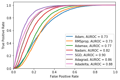
Figure 1: AUROC (based on the MD approach) of models in Table  1 when the OOD dataset is uniform noise.

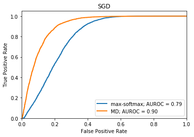
(a)

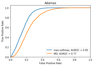
(b)

Figure 2: AUROC for detecting uniform noise (as OOD) by max-softmax and MD over the test set of Fashion-MNIST (as ID). a) It shows AUROC for these two OODD approaches under the SGD optimizer. b) It shows AUROC for these two approaches under the Adamax optimizer. As can be seen, there is not an overall winner.

2 THE PROBLEM STATEMENT

Stochastic gradient descent (SGD) is one of the basic methods used for optimizing objective functions of DNNs. Although it guarantees to converge in convex settings, it is slow. Adaptive gradient methods such as Adam (Kingma and Ba, 2015) have been introduced to reduce the training time. In non-convex settings (e.g., image classification), optimization methods can cause deep models to converge to different local minima. When the classification accuracy of these models is measured based on a test dataset, they can have almost the same accuracy. In this case, it is generally accepted that any of these models can be deployed in real life.

However, these models are different internally. For DNNs, it means weights of these models vary and so they focus on different features to obtain their posteriors. Therefore, an OODD approach based on posteriors or deep features may demonstrate different OODD performance for these models. When this phenomenon happens for an OODD approach, it implies that the approach is not robust to the choice of optimization method.

Table 1 shows the classification accuracy of a convolutional neural network (CNN) trained on the Fashion-MNIST dataset with several well-known optimization methods. As can be seen, they all converge and have similar classification accuracy. Figure 1 shows the Area Under the Receiver Operating Characteristic curve (AUROC) for the uniform noise (as an OOD dataset) based on the MD approach (over logits features) for models in Table 1. There is a large variance for AUROC values even though the models have similar classification accuracy. Please note that the differences in Figure 1 are large, relatively to the typical differences between different OODD approaches. A similar case for MNIST as the ID dataset is depicted in the Appendix, Figure  3.

This characteristic of OODD approaches makes them incomparable unless the effect of the optimization method is incorporated into the comparison. Figure 2(a) shows a comparison of AUROCs calculated by two OODD approaches, max-softmax and MD, under the SGD optimization method. As can be seen, the MD approach has much better AUROC than max-softmax. Figure 2(b) shows AUROCs under Adamax and in which max-softmax has better AUROC than MD. The classification accuracies based on the SGD and Adamax optimization methods are 0.9705 and 0.956, respectively. Thus, the best AUROC is not necessarily related to the best performing classifier when max-softmax is used.

This sensitivity to optimization method may be a possible reason for discrepancies seen among comparison results of published articles in this area. It also highlights the fact that an OODD approach should not be applied blindly to deep models based on its detection performance over a specific ID, OOD, and optimization method. Furthermore, this phenomenon is not limited to AUROC—it can also be observed when OODD approaches are compared using other common metrics as defined in Section 4.3.

In order to incorporate this sensitivity of OODD approaches into OODD metrics and possibly find optimization methods that provide better solutions for OODD approaches, we propose a robustness score that takes into account both the level of detection performance and variation due to different optimization methods. It is described in details in the following section.

3 PROPOSED ROBUSTNESS SCORE

In this section, we formulate our proposed robustness score. We first formulate a robustness score which allows us to properly compare OODD approaches. Then, we expand this formulation to a robustness score that allows finding the best optimization method for a given ID dataset and OODD approach.

Let $X$ be the random variable representing the value of an OODD metric (e.g., AUROC) whose distribution is represented by a probability density function (PDF) $p(x)$. An OODD metric depends on:

1. a given OODD approach $m$ (e.g., max-softmax),

2. an ID dataset $i$ (e.g., MNIST),

3. an OOD dataset $o$ (e.g., Fashion-MNIST).

Thus, we consider its conditional distribution with the PDF $p(x|i,o,m)$ rather than $p(x)$. For conciseness, we denote $\zeta:=(i,o,m)$. Then, $p(x|\zeta)\equiv p(x|i,o,m)$ can be represented by the following mixture PDFs (Bar-Shalom et al., 2002):

$$p(x|\zeta)=\sum_{t\in\mathcal{T}}w^{\zeta,t}\cdot p(x|\zeta,t)$$ (1)

where $\mathcal{T}$ represents a set of optimization methods that are used to train ID models in this paper; $p(x|\zeta,t)$ is the conditional PDF of the OODD metric when the optimization method $t\in\mathcal{T}$ is used to train the ID model; $w^{\zeta,t}\geq 0$ is the weight of $p(x|\zeta,t)$, summing up to unity (i.e., $\sum_{t\in\mathcal{T}}w^{\zeta,t}=1$). Please note that we considered a PDF for a given $\zeta$ and $t$ because there is no guarantee that the ID model with the given optimization method will converge to the same solution all the time. This is due to factors such as randomness in initial weights and data in dataset.

$p(x|\zeta,t)$ is unknown, but its empirical mean and variance can be approximated. This is achieved by training the same ID model with the same optimization method $t$ but different random initial weights. Thus, the mean and variance of $X$ conditioned by $\zeta$ and an optimization method $t$ are empirically approximated by:

$$\mathbb{E}[X|\zeta,t] \approx\mu^{\zeta,t}:=\frac{1}{N}\sum_{j=1}^{N}X^{\zeta,t}_{j}$$ (2)

$$\mathrm{Var}[X|\zeta,t] \approx\mathrm{Var}^{\zeta,t}:=\frac{1}{N}\sum_{j=1}^{N}(\,X^{\zeta,t}_{j}-\mu^{\zeta,t}\,)^{2}$$ (3)

in which $N$ is the number of the ID models trained with the ID dataset $i$ and optimization method $t$ but $N$ different random initial weights. $X^{\zeta,t}_{j}$ represents the OODD metric calculated for the $j$-th ID model of the optimization method $t$.

In order to obtain $w^{\zeta,t}$, we first define confidence score $c^{\zeta,t}$ as:

$$c^{\zeta,t}:=\frac{1}{\sqrt{\mathrm{Var}^{\zeta,t}}+\epsilon}$$ (4)

The confidence score $c^{\zeta,t}$ specifies how much the OODD metric calculated for the ID model trained by the optimization method $t$ can be trusted. $\epsilon>0$ is a sufficiently small value used for numerical stability when $\mathrm{Var}^{\zeta,t}=0$. Then, the normalized form of the confidence score is used to calculate $w^{\zeta,t}$:

$$w^{\zeta,t}=\frac{c^{\zeta,t}}{\sum_{t\in\mathcal{T}}c^{\zeta,t}}$$ (5)

Having the empirical mean $\mu^{\zeta,t}$ and variance $\mathrm{Var}^{\zeta,t}$ of the OODD metric $X$ conditioned by $\zeta$ and $t$, we obtain those of $X$ conditioned only by $\zeta$ using the weights $w^{\zeta,t}$ as (Bar-Shalom et al., 2002):

$$\mathbb{E}[X|\zeta] \approx\mu^{\zeta}:=\sum_{t\in\mathcal{T}}w^{\zeta,t}\cdot\mu^{\zeta,t}$$ (6)

$$\mathrm{Var}[X|\zeta] \approx\mathrm{Var}^{\zeta}$$

$$:=\sum_{t\in\mathcal{T}}w^{\zeta,t}\cdot\big{(}\mathrm{Var}^{\zeta,t}+(\mu^{\zeta}-\mu^{\zeta,t})^{2}\big{)}$$ (7)

The approximated $\mu^{\zeta}$ and $\mathrm{Var}^{\zeta}$ represent how good the corresponding OODD approach according to the OODD metric $X$ on average and how much variation is expected to be seen in the value of $X$, respectively. However, it is still challenging to compare OODD approaches because an OODD approach might have a high mean and high variance while another one might have a slightly less mean but very low variance. Although the former one has a high mean (i.e., better detection), its high variation means that it might show worse results for some optimization methods. The later one gives highly consistent detection performance, but it does not have the best mean.

To accommodate these cases (i.e., the trade-off between mean and variance) and be able to quantitatively compare OODD approaches, we propose using the coefficient of variation (CV) (conditioned by $\zeta$) as a final robustness score, defined as:

$$CV^{\zeta}:=\frac{\sqrt{\mathrm{Var}^{\zeta}}}{\mu^{\zeta}}$$ (8)

The $CV$ takes into account both mean and variance. It favors an OODD approach that has a high mean and low variance for an OODD metric. Therefore, a lower $CV^{\zeta}$ value corresponds to lower variability in the mean of the OODD metric. A robust OODD approach is expected to have a low $CV^{\zeta}$ value. $CV^{\zeta}$ can be calculated for any OODD metrics as we demonstrate it in the next section.

In Figure 2, we demonstrated that an OODD approach can better detect OOD samples if the ID model has been trained with a specific optimization method. $\mu^{\zeta,t}$ and $\mathrm{Var}^{\zeta,t}$ provide a way to find the best optimization method for a given ID, OOD, and OODD approach. We can extend our proposal to finding the best optimization method for a given OODD approach and ID dataset. For this purpose, we consider conditional PDF $p(x|i,m,t)$. For conciseness, we denote $\xi:=(i,m,t)$. Then:

$$p(x|\xi)=\sum_{o\in\mathcal{O}_{i}}w^{\xi,o}\cdot p(x|\xi,o)$$ (9)

$\mathcal{O}_{i}$ is a set of OOD datasets available for the ID dataset $i$. This constraint emerges from not being able to represent all OOD inputs for an ID dataset and also how OODD approaches have been compared in literature. Since $p(x|\xi,o)\equiv p(x|\zeta,t)$ then the mean and variance of $X$ conditioned by $\xi$ and $o$ can be approximated based on (2) and (3). Similarly, $w^{\xi,o}\equiv w^{\zeta,t}$ so $w^{\xi,o}$ can be calculated based on (5). The mean and variance of $X$ conditioned by $\xi$ can then be approximated in a similar way to (6) and (7), but their summation is over $\mathcal{O}_{i}$ instead of $\mathcal{T}$. $CV^{\xi}$, which represents robustness score for optimization method $t$, can now be used to select the best optimization method for a given OODD approach and ID dataset.

4 EXPERIMENTS

We compare several OODD approaches according to our proposed robustness score. Furthermore, we find optimization methods that give better detection performance for a given ID dataset and OODD approach.

4.1 ID AND OOD DATASETS

We use MNIST and Fashion-MNIST (or F-MNIST) as our ID datasets. MNIST is a dataset of $28\times 28$ grayscale images of handwritten digits. It has $60,000$ training images and $10,000$ test images. Fashion-MNIST is similar to the MNIST dataset by also containing $28\times 28$ grayscale images, but the images represent Zalando’s articles (Xiao et al., 2017). We used a convolutional neural network (CNN) with two convolutional layers and two fully connected layers and trained one model for each dataset. The CNN includes dropout layers that allow us to use uncertainty-estimate techniques for the detection of OOD inputs as well.

The OOD datasets of MNIST ($\mathcal{O}_{MNIST}$) are Fashion-MNIST, Omniglot, Gaussian noise, and Uniform noise. The OOD datasets of Fashion-MNIST ($\mathcal{O}_{F-MNIST}$) are MNIST, Omniglot, Gaussian noise, and Uniform noise. We use test datasets of MNIST, Fashion-MNIST, and Omniglot for calculating OODD metrics. We keep the number of ID and OOD inputs the same during evaluation (by randomly selecting data from the larger dataset to match the number of instances in the smaller dataset). The details of the aforementioned OOD datasets are as follows:

• Omniglot contains different handwritten characters from 50 different alphabets. The images have been downsampled to $28\times 28$ images (Lake et al., 2015).

• Gaussian noise includes random normal noise with $\mu=0.5$ and $\sigma=1$, clipped to [0, 1].

• Uniform noise includes random uniform noise between [0, 1].

4.2 OPTIMIZATION METHODS AND TRAINING PROCESS

We used seven optimization methods for our experiments. These methods are Adam (Kingma and Ba, 2015), RMSprop (Tieleman and Hinton, 2012), Adamax (Kingma and Ba, 2015), Nadam (Dozat, 2016), SGD, Adagrad (Duchi et al., 2011), and Adadelta (Zeiler, 2012). The values of parameters used for these optimization methods are depicted in the Appendix, Table 12. They are values recommended by the tools we used for our experiments, which are Tensorflow and Keras.

To train models, we used the early stop technique in which the training process is stopped once no improvements are seen in the validation loss (the chosen patience parameter is 10 epochs). However, the saved model after the training process stops is the model that has the best validation loss. This has been chosen to avoid overfitting.

4.3 OODD METRICS

There are different metrics to evaluate the performance of OODD approaches. We adopted the following metrics (Hendrycks and Gimpel, 2017; Liang et al., 2018).

• FPR at $95\%$ TPR is the probability of an out-of-distribution (i.e., negative) input being misclassified as in-distribution (i.e., positive) input when the true positive rate (TPR) is as high as $95\%$. True positive rate is calculated by $\textit{TPR}=\textit{TP}/(\textit{TP}+\textit{FN})$, where TP and FN denote true positives and false negatives, respectively. The false positive rate (FPR) is computed by $\textit{FPR}=\textit{FP}/(\textit{FP}+\textit{TN})$, where FP and TN denote false positives and true negatives, respectively.

• Detection error calculates the misclassification probability when TPR is $95\%$. It is equal to $0.5*(1-\textit{TPR})+0.5*\textit{FPR}$, where we assume that both positive and negative examples have an equal probability of appearing in the evaluation test.

• AUROC is the Area Under the Receiver Operating Characteristic curve. It is interpreted as the probability that a positive example is assigned a higher detection score than a negative example. An ideal OOD detector expects an AUROC score of $100\%$.

• AUPR is the Area under the Precision-Recall curve. It is a graph reflecting precision equal to $\textit{TP}/(\textit{TP}+\textit{FP})$ and recall equal to $\textit{TP}/(\textit{TP}+\textit{FN})$ against each other. The metric AUPR-In and AUPR-Out represent the area under the precision-recall curve where in-distribution or out-of-distribution images are specified as positives, respectively.

Table 2: $\mu^{\zeta,t}$ and $\mathrm{Var}^{\zeta,t}$ when $\zeta=($MNIST, Fashion-MNIST, max-softmax$)$ and $t=$Adam. $\downarrow$ indicates that lower values are better; $\uparrow$ indicates that higher values are better.

Opt. method	FPR at 95% TPR $\downarrow$	Detection error $\downarrow$	AUROC $\uparrow$	AUPR Out $\uparrow$	AUPR In $\uparrow$
Adam	10.24	7.61	97.728	97.981	97.483
Adam	7.47	6.225	97.834	98.272	97.176
Adam	16.5	10.735	96.421	96.705	96.018
Adam	7.57	6.18	98.195	98.482	97.897
Adam	15.32	10.11	96.554	96.671	96.277
$\mu^{\zeta,t}|\mathrm{Var}^{\zeta,t}$	11.42 | 14.567	8.172 | 3.68	97.346 | 0.518	97.622 | 0.607	96.97 | 0.51

Table 3: $\mu^{\zeta}$ and $\mathrm{Var}^{\zeta}$ when $\zeta=($MNIST, Fashion-MNIST, max-softmax$)$ and $\mathcal{T}=\{$Adam, RMSprop, Adamax, Nadam, SGD, Adagrad, Adadelta$\}$. $\downarrow$ indicates that lower values are better; $\uparrow$ indicates that higher values are better.

Opt. Method	FPR at 95% TPR $\mu\downarrow|\mathrm{Var}\downarrow$	Detection error $\mu\downarrow|\mathrm{Var}\downarrow$	AUROC $\mu\uparrow|\mathrm{Var}\downarrow$	AUPR Out $\mu\uparrow|\mathrm{Var}\downarrow$	AUPR In $\mu\uparrow|\mathrm{Var}\downarrow$
Adam	11.42 | 14.567	8.172 | 3.68	97.346 | 0.518	97.622 | 0.607	96.97 | 0.51
RMSprop	7.804 | 5.236	6.319 | 1.446	97.988 | 0.256	98.278 | 0.276	97.609 | 0.344
Adamax	8.844 | 4.348	6.897 | 1.096	97.608 | 0.156	97.971 | 0.129	97.111 | 0.224
Nadam	9.018 | 0.886	6.968 | 0.231	97.751 | 0.022	98.054 | 0.026	97.349 | 0.118
SGD	7.236 | 3.911	6.042 | 1.039	98.026 | 0.204	98.385 | 0.182	97.56 | 0.212
Adagrad	8.56 | 3.697	6.721 | 0.972	97.685 | 0.233	98.103 | 0.176	97.122 | 0.351
Adadelta	8.252 | 9.935	6.572 | 2.634	97.88 | 0.503	98.191 | 0.455	97.48 | 0.664
$\mu^{\zeta}|\mathrm{Var}^{\zeta}$	8.634 | 5.506	6.769 | 1.445	97.756 | 0.219	98.089 | 0.216	97.315 | 0.349

Table 4: $\mu^{\zeta}$ and $\mathrm{Var}^{\zeta}$ when $\zeta=($MNIST, Fashion-MNIST, $m)$ and $m\in\{$max-softmax, ODIN,MD, Entropy, Margin, MC-D, MI $\}$. $\downarrow$ indicates that lower values are better; $\uparrow$ indicates that higher values are better.

OODD approaches	FPR at 95% TPR $\mu\downarrow|\mathrm{Var}\downarrow$	Detection error $\mu\downarrow|\mathrm{Var}\downarrow$	AUROC $\mu\uparrow|\mathrm{Var}\downarrow$	AUPR Out $\mu\uparrow|\mathrm{Var}\downarrow$	AUPR In $\mu\uparrow|\mathrm{Var}\downarrow$
max-softmax	8.634 | 5.506	6.769 | 1.445	97.756 | 0.219	98.089 | 0.216	97.315 | 0.349
ODIN	4.932 | 3.081	4.84 | 0.983	98.944 | 0.12	99.036 | 0.104	98.87 | 0.137
MD	64.707 | 31.994	34.837 | 7.966	69.108 | 19.587	75.163 | 14.237	62.276 | 18.813
Entropy	8.549 | 5.467	6.728 | 1.442	97.944 | 0.22	98.195 | 0.202	97.703 | 0.327
Margin	8.777 | 5.52	6.842 | 1.448	97.625 | 0.214	98.023 | 0.222	96.855 | 0.344
MC-D	8.218 | 4.33	6.536 | 1.209	97.868 | 0.221	98.213 | 0.191	97.465 | 0.298
MI	8.817 | 4.748	6.812 | 1.285	97.238 | 0.224	97.857 | 0.199	96.125 | 0.458

Table 5: The $CV^{\zeta}$ values for the $\mu^{\zeta}$ and $\mathrm{Var}^{\zeta}$ in Table 4. Since better FPR@95%TPR and detection error should have low mean, we use the inverse of $\mathrm{Var}^{\zeta}$ to calculate $CV^{\zeta}$ to have consistent score among all other metrics. The bold values highlights the most robust OODD approach for the given metric. $\downarrow$ indicates that lower values are better.

OODD approaches	FPR at 95% TPR $\mu*\sqrt{\mathrm{Var}}\downarrow$	Detection error $\mu*\sqrt{\mathrm{Var}}\downarrow$	AUROC $\sqrt{\mathrm{Var}}/\mu\downarrow$	AUPR Out$\sqrt{\mathrm{Var}}/\mu\downarrow$	AUPR In $\sqrt{\mathrm{Var}}/\mu\downarrow$
max-softmax	20.258	8.138	0.005	0.005	0.006
ODIN	8.657	4.797	0.003	0.003	0.004
MD	365.988	98.313	0.064	0.05	0.07
Entropy	19.99	8.082	0.005	0.005	0.006
Margin	20.62	8.232	0.005	0.005	0.006
MC-D	17.104	7.191	0.005	0.004	0.006
MI	19.214	7.726	0.005	0.005	0.007

Table 6: Best OODD approaches based on FPR@95%TPR for different ID and OOD datasets.

ID	OOD	OODD approach
	F-MNIST	ODIN
MNIST	Omniglot	MC-D
	Gaussian	ODIN
	Uniform	ODIN
	MNIST	MD
F-MNIST	Omniglot	MI
	Gaussian	ODIN
	Uniform	MI

4.4 OODD APPROACHES

In this paper, we focus on OODD approaches that apply to already-trained models and are easiest to incorporate into existing application. There are other OODD approaches such as generative or classifier-based approaches (Pidhorskyi et al., 2018; Wang et al., 2017; Lee et al., 2018b) that require models to be retrained. We consider these as our future work. The OODD approaches used in our experiments are max-softmax (Hendrycks and Gimpel, 2017), ODIN (without input preprocessing and $T$=1000) (Liang et al., 2018), Mahalanobis Distance (MD) based on logits features (without input preprocessing) (Lee et al., 2018a), and Entropy, Margin, the MC-dropout (MC-D) (Gal and Ghahramani, 2016), and Mutual Information (MI) (Gal et al., 2017).

4.5 ROBUSTNESS SCORES OF OODD APPROACHES

Table  2 shows the means $\mu^{\zeta,t}$ and variances $\mathrm{Var}^{\zeta,t}$ of different OODD metrics (the last row) for MNIST as ID, Fashion-MNIST as OOD, max-softmax as the OODD approach, and Adam as the optimization method. For example, the mean value for FPR@95%TPR is 11.42 and we might have better or worse FPR@95%TPR under a certain solution obtained by Adam because of the high variance, which is 14.567. To approximate the means and variances based on (2) and (3), OODD metrics are calculated for five models (each represented by a row in the middle cell) with different initial weights. FPR@95%TPR and detection error show the highest variance among other metrics. High variance for other OODD metrics can also be seen in our other experiment in Table  13 in the Appendix.

Table  3 depicts the means $\mu^{\zeta}$ and variances $\mathrm{Var}^{\zeta}$ of different OODD metrics (the last row) when $\zeta=($MNIST, Fashion-MNIST, max-softmax$)$. For example, the mean value for FPR@95%TPR is 8.63 and we expect to see some difference in the performance due to its variance, which is 5.506. The means and variances are regardless of which optimization method is selected to train the ID model. To approximate these moments (based on (6) and (7)), we use the mean and variance of the metrics calculated for seven optimization methods (each represented by a row in the middle cell) in the same way as depicted in Table  2. We can observe that SGD has the lowest mean for FPR@95%TPR, but it does not have the lowest variance. Nadam has the lowest variance but not the highest mean. Adam has the highest mean, but also the highest variance.

The mean and variance of OODD metrics for different OODD approaches are depicted in Table 4. MD shows a poor detection performance in comparison to others, but in our other experiments in the Appendix (Table  15), MD shows good performance. This can be related to the fact that the distribution of features for the logits layer in the MNIST model may not follow a multivariate Gaussian distribution. Therefore, the OOD score comes our of MD is not reliable for separating ID and OOD inputs. The MD approach may also be an ID dataset dependent.

To find the best OODD approach based on their mean and variance, the $CV^{\zeta}$ values of different metrics and OODD approaches from Table 4 are shown in Table  5. ODIN shows the lowest $CV^{\zeta}$ scores for all OODD metrics and can be considered as a robust OODD approach for MNIST as ID and Fashion-MNIST as OOD. A summary of the best OODD approach for other ID and OO datasets based on FPR@95%TPR is depicted in Table 6.

We can observe that ODIN performs better than others on average; however, there is not a perfect OODD approach. This is opposite to what we can see in many published papers where authors compare their proposed OODD approach with others and theirs outperforms all others. This demonstrates how our robustness score could incorporate the effect of optimization methods in OODD metrics for a sound comparison.

4.6 ROBUST OPTIMIZATION METHODS

Table 7 show the mean $\mu^{\xi}$ and variance of $\mathrm{Var}^{\xi}$ of different OODD metrics (the last row) when $\xi=($MNIST, max-softmax, Adam$)$. These values show the quality of solutions offered by Adam for detecting different kinds of OOD datasets for a given ID and OODD approach. The moments are approximated over metrics calculated for different OOD datasets. These metrics (rows in the middle cell) are approximated in similar way as in Table 2. Table 8 shows $\mu^{\xi}$ and $\mathrm{Var}^{\xi}$ when $\xi=($MNIST, max-softmax, $t)$ and $t$ can be one of the seven optimization methods. To find the best optimization method for a given ID and OODD approach based on the means and variances, the $CV^{\xi}$ values are shown in Table 9. SGD and Nadam have the lowest scores for all metrics. It means the MNIST models trained with these optimization methods can provide better solutions for detecting OOD inputs when max-softmax is used as the OODD approach. Table 10 shows a summary of top-two optimization methods based on FPR@95%TPR for two ID datasets and several OODD approaches.

Table 7: $\mu^{\xi}$ and $\mathrm{Var}^{\xi}$ when $\xi=($MNIST, max-softmax, Adam$)$ and $\mathcal{O}_{MNIST}=\{$Fashion-MNIST, Omniglot, Gaussian, Uniform$\}$

OOD	FPR at 95% TPR $\mu\downarrow|\mathrm{Var}\downarrow$	Detection error $\mu\downarrow|\mathrm{Var}\downarrow$	AUROC $\mu\uparrow|\mathrm{Var}\downarrow$	AUPR Out $\mu\uparrow|\mathrm{Var}\downarrow$	AUPR In $\mu\uparrow|\mathrm{Var}\downarrow$
F-MNIST	11.42 | 14.567	8.172 | 3.68	97.346 | 0.518	97.622 | 0.607	96.97 | 0.51
Omniglot	6.08 | 1.373	5.246 | 0.547	98.205 | 0.127	98.613 | 0.079	97.559 | 0.319
Gaussian	1.146 | 1.067	0.99 | 0.343	99.348 | 0.543	99.62 | 0.167	98.073 | 5.747
Uniform	3.368 | 1.663	2.757 | 0.854	98.406 | 0.567	99.003 | 0.19	96.415 | 5.02
$\mu^{\xi}|\mathrm{Var}^{\xi}$	4.162 | 11.733	3.437 | 6.649	98.282 | 0.78	98.82 | 0.579	97.257 | 1.683

Table 8: $\mu^{\xi}$ and $\mathrm{Var}^{\xi}$ when $\xi$ = (MNIST,max-softmax, $t$), $t\in\mathcal{T}=\{$Adam, RMSprop, Adamax, Nadam, SGD, Adagrad, Adadelta$\}$ and $\mathcal{O}_{MNIST}=\{$Fashion-MNIST, Omniglot, Gaussian, Uniform$\}$

Opt. method	FPR at 95% TPR $\mu\downarrow|\mathrm{Var}\downarrow$	Detection error $\mu\downarrow|\mathrm{Var}\downarrow$	AUROC $\mu\uparrow|\mathrm{Var}\downarrow$	AUPR Out $\mu\uparrow|\mathrm{Var}\downarrow$	AUPR In $\mu\uparrow|\mathrm{Var}\downarrow$
Adam	4.162 | 11.733	3.437 | 6.649	98.282 | 0.78	98.82 | 0.579	97.257 | 1.683
RMSprop	4.059 | 18.879	3.497 | 9.398	98.443 | 1.862	98.895 | 1.189	97.696 | 4.433
Adamax	3.487 | 10.255	3.305 | 6.656	98.674 | 0.88	99.058 | 0.609	98.014 | 1.364
Nadam	2.404 | 9.64	2.495 | 6.995	99.225 | 0.86	99.476 | 0.518	99.293 | 1.018
SGD	2.82 | 6.985	2.578 | 5.025	98.849 | 0.632	99.22 | 0.404	98.161 | 1.188
Adagrad	4.346 | 9.209	3.835 | 5.834	98.417 | 0.816	98.843 | 0.502	97.702 | 2.285
Adadelta	4.188 | 12.394	3.707 | 6.758	98.406 | 1.241	98.863 | 0.716	97.554 | 3.719

Table 9: The $CV^{\xi}$ values for the $\mu^{\xi}$ and $\mathrm{Var}^{\xi}$ efined in Table 8. Since better FPR@95%TPR and detection error should have low mean, we use the inverse of $\mathrm{Var}^{\xi}$ to calculate $CV^{\xi}$ to have consistent score among all other metrics. The bold values highlights the most robust optimization method for the given metric. $\downarrow$ indicates that lower values are better.

Opt. methods	FPR at 95% TPR $\mu*\sqrt{\mathrm{Var}}\downarrow$	Detection error $\mu*\sqrt{\mathrm{Var}}\downarrow$	AUROC $\sqrt{\mathrm{Var}}/\mu\downarrow$	AUPR Out $\sqrt{\mathrm{Var}}/\mu\downarrow$	AUPR In $\sqrt{\mathrm{Var}}/\mu\downarrow$
Adam	14.258	8.867	0.009	0.008	0.013
RMSprop	17.641	10.725	0.014	0.011	0.022
Adamax	11.169	8.529	0.01	0.008	0.012
Nadam	7.468	6.602	0.009	0.007	0.01
SGD	7.456	5.782	0.008	0.006	0.011
Adagrad	13.193	9.264	0.009	0.007	0.015
Adadelta	14.749	9.641	0.011	0.009	0.02

Table 10: Top-two optimization methods based on FPR@95%TPR for OODD approaches.

OODD approach	MNIST	Fashion-MNIST
max-softmax	SGD,Nadam	RMSProp,SGD
ODIN	Nadam,Adamax	RMSProp,Nadam
MD	MSprop,Adagrad	Nadam,Adagrad
Entropy	Nadam,SGD	RMSProp,Nadam
Margin	Nadam,SGD	RMSProp,SGD
MC-D	Nadam,SGD	RMSProp,Adamax
MI	Adagrad,Nadam	Adamax,Adadelta

4.7 DISCUSSION

The robustness of OODD approaches under optimization methods is a significant aspect that needs to be incorporated into OOD detection metrics. We proposed a robustness score that takes into account the effect of optimization methods. It gives equal importance to both mean and variance. However, we can imagine in some context and application it might be preferred to pay more attention to either mean or variance. In that case, instead of using the $CV$ (8), a custom formula can be adopted.

We calculated our robustness score for five OODD metrics and this approach can be easily adapted for any custom OODD metric. We specifically focused on FPR@95%TPR to describe the application of our robustness score and our conclusions are based on this metric. Focusing on other OODD metrics can change some of our conclusions (e.g., the best optimization method for an OODD approach). Our goal in this paper is not to extensively compare OODD approaches or recommend one. The goal is to demonstrate the importance of optimization methods in the domain of OODD and suggest a way to incorporate it into OODD metrics.

We observed that some OODD approaches better detect OOD inputs if the ID model has been trained with a specific optimization method. We experimentally found the best-performing optimization methods for several OODD approaches based on FPR@95%TPR. However, it is still unclear what solutions these optimization methods provide that cause these approaches to work better.

One hypothesis is that these optimization methods achieve solutions that generalize better. Thus, OODD approaches are able to better detect OOD and ID inputs. Wilson et al. (2017) studied the effect of adaptive optimization methods and SGD on the generalization of solutions. They found that solutions offered by SGD generalize better. SGD is among the top optimization methods found for OODD approaches in this paper. However, it is not the best for all ID and OODD approaches. We believe this aspect of optimization methods requires rigorous studies.

The second hypothesis is that an OODD approach has specific requirements on the ID model to demonstrate its best detection performance. For example, the MD approach requires the class-conditional distribution of features to be Gaussian. This condition might happen under specific optimization methods. Max-softmax and uncertainty-based approaches need confident models and might happen under specific optimization methods, too. Therefore, it is important for OODD approaches to precisely define the conditions under which they achieve their claimed performance and provide appropriate tests for practitioners to apply before using the approach.

Please note that one could evaluate pairs, i.e., a detection appraoch and optimizer; by doing this, the winning approach is changed for every ID and OOD data pair. Therefore, it becomes challenging to compare OODD approaches because there is no winner. Our weighted average also applies to pairwise evaluation (to average out the effects over different ID and OOD data combinations) and can show the overall robust OODD approach with a statistically rigorous formulation. Moreover, when comparing OODD approaches applied to an already-trained ID model, the ID model should be kept the same for a fair comparison. Thus, a pairwise comparison might not be an option for this case.

Our robustness score evaluates OODD approaches over several optimization methods, however, someone may decide to treat optimizer selection as hyperparameter tuning. This can be performed in two ways: i) We can tune it to improve classification performance; the improvement is typically small. We could not observe in our experiments that there is a strong correlation between the slightly improved classification accuracy and OODD performance. This tuning will not affect the issue at hand and our robustness score. ii) We can tune the optimization for a specific OODD approach until we get the best OODD performance. This might cause the model to have a bias toward some OOD datasets; however, it can be helpful when a user has already selected an OODD approach and wants to get the maximum OODD performance out of it. This case can bring up the pairwise comparison idea (mentioned in the previous paragraph).

We also attempted to find a correlation between the final minima and OOD performance. We looked at published articles in the field of optimization methods to see if there are any insights about the properties of the final minima that we could apply. Unfortunately, we could not find any relevant work. We also tried to apply statistical tests to feature spaces of the final minima to understand trends or patterns, but we could not see any patterns. Some of our statistical tests failed due to the sparsity of neurons.

Our robustness score is a statistically rigorous formulation to decide which approach is robust in general w.r.t optimizers. An OODD approach can have the best detection performance for a specific combination of optimizer, ID and OOD data. If we compare detection approaches by selecting the best optimizer for each approach, the comparison would be valid only for that specific combination of ID and OOD data. Our robustness score accounts for all these combinations and shows which approach performs well in general. It also considers the tradeoff between mean and variance for better comparison.

Finally, in our experiments, we trained limited number of ID and OOD models with different optimization methods and fixed parameters (e.g., learning rate). It is possible that changing such parameters may affect some of the results; however, the general approach to incorporate varying optimization methods in OODD performance assessment remains unaffected.

5 CONCLUSION AND FUTURE WORK

In this paper, we concentrated on the robustness of OODD approaches for deep classifiers trained with different optimization methods and achieving the same classification accuracy. OODD approaches can have varying detection performance when they are applied to such classifiers. Thus, a comparison of OODD approaches under one optimization method cannot result in sound comparison because one OODD approach can outperform others under such an optimization method.

We proposed a robustness score which takes into account variations in OODD metrics due to optimization methods. We also proposed a way to find best-performing optimization methods for OODD approaches. We compared several OODD approaches based on our proposed robustness score and find their best-performing optimization methods. The result reveals that there is not a winner among several OODD approaches investigated in this paper when the effect of optimization methods is considered. It also shows that it is feasible to have better OODD for a specific OODD approach just by using the right optimization method for a given ID dataset.

As future work, it is interesting to investigate whether or not the issue indicated in this paper stands for other OODD approaches that need ID models to be retrained. We also want to investigate the effect of optimization methods’ parameters on the performance of OODD approaches.

Appendix

Table 11: Test classification accuracy of a CNN for MNIST under different optimization methods.

Optimizer	accuracy
Adam	0.9995
RMSprop	0.9984
Adamax	0.9998
Nadam	0.9994
SGD	0.9983
Adagrad	0.9992
Adadelta	0.9984

Figure 3: AUROC (based on the MD approach) of models in Table  11 when the OOD dataset is uniform noise.

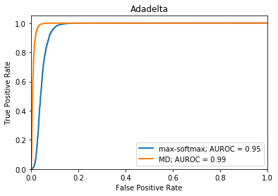
(a)

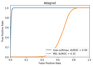
(b)

Figure 4: AUROC for detecting uniform noise (as OOD) by max-softmax and MD over the test set of MNIST (as ID). a) It shows AUROC for these two OODD approaches under the Adadelta optimizer. b) It shows AUROC for these two approaches under the Adamax optimizer. As seen, there is not a winner.

Table 12: Values of parameters for optimization methods used in our experiments. The parameters are based on the default values used in Keras.

Methods	Parameters and their values
Adam	lr=0.001, beta_1=0.9, beta_2=0.999, epsilon=None, decay=0.0, amsgrad=False
RMSprop	lr=0.001, rho=0.9, epsilon=None, decay=0.0
Adamax	lr=0.001, beta_1=0.9, beta_2=0.999, epsilon=None, decay=0.0
Nadam	lr=0.001, beta_1=0.9, beta_2=0.999, epsilon=None, schedule_decay=0.004
SGD	lr=0.01, momentum=0.0, decay=0.0, nesterov=False
Adagrad	lr=0.01, epsilon=None, decay=0.0
Adadelta	lr=0.1, rho=0.95, epsilon=None, decay=0.0

Table 13: $\mu^{\zeta,t}$ and $\mathrm{Var}^{\zeta,t}$ when $\zeta=($Fashion-MNIST, MNIST, max-softmax$)$ and $t=$Adam. $\downarrow$ indicates that lower values are better; $\uparrow$ indicates that higher values are better.

Opt. method	FPR at 95% TPR $\downarrow$	Detection error $\downarrow$	AUROC $\uparrow$	AUPR Out $\uparrow$	AUPR In $\uparrow$
Adam	77.356	41.465	64.109	67.773	61.175
Adam	69.035	37.01	74.141	76.379	72.005
Adam	68.165	36.67	70.267	74.257	65.598
Adam	71.815	50.0	68.161	71.84	65.366
Adam	70.663	38.435	67.484	71.606	63.916
$\mu^{\zeta,t}|\mathrm{Var}^{\zeta,t}$	71.407 | 10.45	40.716 | 24.412	68.832 | 10.964	72.371 | 8.326	65.612 | 12.699

Table 14: $\mu^{\zeta}$ and $\mathrm{Var}^{\zeta}$ when $\zeta=($Fashion-MNIST, MNIST, max-softmax$)$ and $\mathcal{T}=\{$Adam, RMSprop, Adamax, Nadam, SGD, Adagrad, Adadelta$\}$. $\downarrow$ indicates that lower values are better; $\uparrow$ indicates that higher values are better.

Opt. method	FPR at 95% TPR $\mu\downarrow|\mathrm{Var}\downarrow$	Detection error $\mu\downarrow|\mathrm{Var}\downarrow$	AUROC $\mu\uparrow|\mathrm{Var}\downarrow$	AUPR Out $\mu\uparrow|\mathrm{Var}\downarrow$	AUPR In $\mu\uparrow|\mathrm{Var}\downarrow$
Adam	71.407 | 10.45	40.716 | 24.412	68.832 | 10.964	72.371 | 8.326	65.612 | 12.699
RMSprop	74.546 | 80.274	42.493 | 40.274	67.514 | 45.959	71.179 | 34.877	64.166 | 37.597
Adamax	82.092 | 82.584	45.235 | 34.119	64.323 | 54.821	67.134 | 41.227	62.532 | 55.91
Nadam	80.101 | 43.682	45.573 | 29.507	65.14 | 15.893	67.955 | 15.701	62.74 | 13.509
SGD	76.609 | 29.081	46.088 | 28.054	67.636 | 15.044	70.545 | 13.598	64.531 | 15.677
Adagrad	87.011 | 26.786	50.0 | 0.0	60.492 | 24.628	63.956 | 14.025	58.995 | 17.294
Adadelta	74.469 | 53.346	42.422 | 42.281	68.537 | 8.124	71.838 | 10.378	65.591 | 5.486
$\mu^{\zeta}|\mathrm{Var}^{\zeta}$	77.387 | 67.105	49.993 | 0.08	66.469 | 27.413	69.489 | 25.281	63.71 | 22.495

Table 15: $\mu^{\zeta}$ and $\mathrm{Var}^{\zeta}$ when $\zeta=($Fashion-MNIST, MNIST, $m)$ and $m\in\{$max-softmax, ODIN,MD, Entropy, Margin, MC-D, MI $\}$. $\downarrow$ indicates that lower values are better; $\uparrow$ indicates that higher values are better.

OODD approaches	FPR at 95% TPR $\mu\downarrow|\mathrm{Var}\downarrow$	Detection error $\mu\downarrow|\mathrm{Var}\downarrow$	AUROC $\mu\uparrow|\mathrm{Var}\downarrow$	AUPR Out $\mu\uparrow|\mathrm{Var}\downarrow$	AUPR In $\mu\uparrow|\mathrm{Var}\downarrow$
max-softmax	77.387 | 67.105	49.993 | 0.08	66.469 | 27.413	69.489 | 25.281	63.71 | 22.495
ODIN	75.435 | 71.953	40.22 | 18.058	74.588 | 41.227	73.864 | 49.736	74.426 | 36.183
MD	9.877 | 9.661	7.385 | 2.576	97.946 | 0.488	98.243 | 0.359	97.57 | 0.708
Entropy	76.023 | 48.192	40.513 | 12.051	67.435 | 28.977	69.975 | 32.341	66.06 | 27.431
Margin	76.836 | 62.898	42.105 | 30.326	66.139 | 25.828	69.361 | 25.381	62.046 | 17.658
MC-D	55.175 | 71.958	30.08 | 18.0	82.466 | 11.97	83.791 | 14.493	81.062 | 12.711
MI	48.207 | 154.677	26.596 | 38.667	92.402 | 8.235	90.691 | 14.23	93.955 | 4.814

References

- Nguyen et al. (2014) Anh Mai Nguyen, Jason Yosinski, and Jeff Clune. Deep neural networks are easily fooled: High confidence predictions for unrecognizable images. CoRR, abs/1412.1897, 2014.
- Hendrycks and Gimpel (2017) Dan Hendrycks and Kevin Gimpel. A baseline for detecting misclassified and out-of-distribution examples in neural networks. In ICLR, 2017.
- DeVries and Taylor (2018) Terrance DeVries and Graham W. Taylor. Learning confidence for out-of-distribution detection in neural networks. arXiv preprint arXiv:1802.04865, 2018.
- Liang et al. (2018) Shiyu Liang, Yixuan Li, and R. Srikant. Principled detection of out-of-distribution examples in neural networks. In ICLR, 2018.
- Lee et al. (2018a) Kimin Lee, Kibok Lee, Honglak Lee, and Jinwoo Shin. A simple unified framework for detecting out-of-distribution samples and adversarial attacks. In NeurIPS, NIPS’18, pages 7167–7177, 2018a.
- Ren et al. (2019) Jie Ren, Peter J. Liu, Emily Fertig, Jasper Snoek, Ryan Poplin, Mark A. DePristo, Joshua V. Dillon, and Balaji Lakshminarayanan. Likelihood ratios for out-of-distribution detection. CoRR, abs/1906.02845, 2019.
- Kingma and Ba (2015) Diederik P. Kingma and Jimmy Lei Ba. Adam: A method for stochastic optimization. In International Conference for Learning Representations, pages 309–318, 2015.
- Bar-Shalom et al. (2002) Yaakov Bar-Shalom, Thiagalingam Kirubarajan, and X.-Rong Li. Estimation with Applications to Tracking and Navigation. John Wiley & Sons, Inc., USA, 2002. ISBN 0471221279.
- Xiao et al. (2017) Han Xiao, Kashif Rasul, and Roland Vollgraf. Fashion-mnist: a novel image dataset for benchmarking machine learning algorithms. CoRR, abs/1708.07747, 2017. URL http://arxiv.org/abs/1708.07747.
- Lake et al. (2015) Brenden M. Lake, Ruslan Salakhutdinov, and Joshua B. Tenenbaum. Human-level concept learning through probabilistic program induction. Science, 350(6266):1332–1338, 2015.
- Tieleman and Hinton (2012) T. Tieleman and G. Hinton. Lecture 6.5—RmsProp: Divide the gradient by a running average of its recent magnitude. COURSERA: Neural Networks for Machine Learning, 2012.
- Dozat (2016) Timothy Dozat. Incorporating nesterov momentum into. In ICLR workshop, 2016.
- Duchi et al. (2011) John Duchi, Elad Hazan, and Yoram Singer. Adaptive subgradient methods for online learning and stochastic optimization. J. Mach. Learn. Res., 12:2121–2159, July 2011. ISSN 1532-4435.
- Zeiler (2012) Matthew D. Zeiler. ADADELTA: an adaptive learning rate method. CoRR, abs/1212.5701, 2012.
- Pidhorskyi et al. (2018) S. Pidhorskyi, R. Almohsen, D. A. Adjeroh, and G. Doretto. Generative probabilistic novelty detection with adversarial autoencoders. In Advances in neural information processing systems (NeuRIPS), 2018.
- Wang et al. (2017) William Wang, Angelina Wang, Aviv Tamar, Xi Chen, and Pieter Abbeel. Safer classification by synthesis. CoRR, abs/1711.08534, 2017.
- Lee et al. (2018b) Kimin Lee, Honglak Lee, Kibok Lee, and Jinwoo Shin. Training confidence-calibrated classifiers for detecting out-of-distribution samples. In ICLR, 2018b.
- Gal and Ghahramani (2016) Yarin Gal and Zoubin Ghahramani. Dropout as a bayesian approximation: Representing model uncertainty in deep learning. In Proceedings of The 33rd International Conference on Machine Learning, pages 1050–1059, 2016.
- Gal et al. (2017) Yarin Gal, Riashat Islam, and Zoubin Ghahramani. Deep bayesian active learning with image data. CoRR, abs/1703.02910, 2017.
- Wilson et al. (2017) Ashia C Wilson, Rebecca Roelofs, Mitchell Stern, Nati Srebro, and Benjamin Recht. The Marginal Value of Adaptive Gradient Methods in Machine Learning. In NeurIPS, pages 4148–4158, 2017.