Sparse Convex Optimization via Adaptively Regularized Hard Thresholding

Abstract

The goal of Sparse Convex Optimization is to optimize a convex function $f$ under a sparsity constraint $s\leq s^{*}\gamma$, where $s^{*}$ is the target number of non-zero entries in a feasible solution (sparsity) and $\gamma\geq 1$ is an approximation factor. There has been a lot of work to analyze the sparsity guarantees of various algorithms (LASSO, Orthogonal Matching Pursuit (OMP), Iterative Hard Thresholding (IHT)) in terms of the Restricted Condition Number $\kappa$. The best known algorithms guarantee to find an approximate solution of value $f(x^{*})+\epsilon$ with the sparsity bound of $\gamma=O\left(\kappa\min\left\{\log\frac{f(x^{0})-f(x^{*})}{\epsilon},\kappa\right\}\right)$, where $x^{*}$ is the target solution. We present a new Adaptively Regularized Hard Thresholding (ARHT) algorithm that makes significant progress on this problem by bringing the bound down to $\gamma=O(\kappa)$, which has been shown to be tight for a general class of algorithms including LASSO, OMP, and IHT. This is achieved without significant sacrifice in the runtime efficiency compared to the fastest known algorithms. We also provide a new analysis of OMP with Replacement (OMPR) for general $f$, under the condition $s>s^{*}\frac{\kappa^{2}}{4}$, which yields Compressed Sensing bounds under the Restricted Isometry Property (RIP). When compared to other Compressed Sensing approaches, it has the advantage of providing a strong tradeoff between the RIP condition and the solution sparsity, while working for any general function $f$ that meets the RIP condition.

1 Introduction

Sparse Convex Optimization is the problem of optimizing a convex objective, while constraining the sparsity of the solution (its number of non-zero entries). Variants and special cases of this problem have been studied for many years, and there have been countless applications in Machine Learning, Signal Processing, and Statistics. In Machine Learning it is used to regularize models by enforcing parameter sparsity, since a sparse set of parameters often leads to better model generalization. Furthermore, in a lot of large scale applications the number of parameters of a trained model is a significant factor in computational efficiency, thus improved sparsity can lead to improved time and memory performance. In applied statistics, a single extra feature translates to a real cost from increasing the number of samples. In Compressed Sensing, finding a sparse solution to a Linear Regression problem can be used to significantly reduce the sample size for the recovery of a target signal. In the context of these applications, decreasing sparsity by even a small amount while not increasing the accuracy can have a significant impact.

Sparse Optimization

Given a function $f:\mathbb{R}^{n}\rightarrow\mathbb{R}$ and any $s^{*}$-sparse (unknown) target solution $x^{*}$, the Sparse Optimization problem is to find an $s$-sparse solution $x$, i.e. a solution with at most $s$ non-zero entries, such that $f(x)\leq f(x^{*})+\epsilon$ and $s\leq s^{*}\gamma$, where $\epsilon>0$ is a desired accuracy and $\gamma\geq 1$ is an approximation factor for the target sparsity. Even if $f$ is a convex function, the sparsity constraint makes this problem non-convex, and it has been shown that it is an intractable problem, even when $\gamma=O\left(2^{\log^{1-\delta}n}\right)$ and $f$ is the Linear Regression objective [Nat95, FKT15]. However, this worst-case behavior is not observed in practice, and so a large body of work has been devoted to the analysis of algorithms under the assumption that the restricted condition number $\kappa_{s+s^{*}}=\frac{\rho_{s+s^{*}}^{+}}{\rho_{s+s^{*}}^{-}}$ (or just $\kappa=\frac{\rho^{+}}{\rho^{-}}$) of $f$ is bounded [Nat95, SSSZ10, Zha11, BRB13, LYF14, JTK14, YLZ16, SL17a, SL17b, JTK14, SGJN18]. Note: Here, $\rho_{s+s^{*}}^{+}$ is the maximum smoothness constant of any restriction of $f$ on an $(s+s^{*})$-sparse subset of coordinates and $\rho_{s+s^{*}}^{-}$ is the minimum strong convexity constant of any restriction of $f$ on an $(s+s^{*})$-sparse subset of coordinates.

The first algorithm for this problem, often called Orthogonal Matching Pursuit (OMP) or Greedy, was analyzed by [Nat95] for Linear Regression, and subsequently for general $f$ by [SSSZ10], obtaining the guarantee that the sparsity of the returned solution is $O\left(s^{*}\kappa\log\frac{f(x^{0})-f(x^{*})}{\epsilon}\right)$ . In applications where having low sparsity is crucial, the dependence of sparsity on the required accuracy $\epsilon$ is undesirable. The question of whether this dependence can be removed was answered positively [SSSZ10, JTK14] giving a sparsity guarantee of $O(s^{*}\kappa^{2})$. As remarked in [SSSZ10], this bound sacrifices the linear dependence on $\kappa$, while removing the dependence on $\epsilon$ and $f(x^{0})-f(x^{*})$.

Since then, there has been some work on improving these results by introducing non-trivial assumptions, such as the target solution $x^{*}$ being close to globally optimal. More specifically, [Zha11] defines the Restricted Gradient Optimal Constant (RGOC) at level $s$, $\zeta_{s}$ (or just $\zeta$) as the $\ell_{2}$ norm of the top-$s$ elements in $\nabla f(x^{*})$ and analyzes an algorithm that gives sparsity $s=O\left(s^{*}\kappa\log\left(s^{*}\kappa\right)\right)$, and such that $f(x)\leq f(x^{*})+O(\zeta^{2}/\rho^{-})$. [SGJN18] strengthens this bound to $f(x)\leq f(x^{*})+O(\zeta^{2}/\rho^{+})$ with sparsity $s=O\left(s^{*}\kappa\log\kappa\right)$. However, this means that $f(x)$ might be much larger than $f(x^{*})+\epsilon$ in general. To the best of our knowledge, no improvement has been made over the $O\left(s^{*}\min\left\{\kappa\frac{f(x^{0})-f(x^{*})}{\epsilon},\kappa^{2}\right\}\right)$ bound in the general case.

Another line of work studies a maximization version of the sparse convex optimization problem as well as its generalizations for matroid constraints [ABF⁺16, EDFK17, CFK18].

Sparse Solution and Support Recovery

Often, as is the case in Compressed Sensing, one needs a guarantee on the closeness of the solution $x$ to the target solution $x^{*}$ in absolute terms, rather than in terms of the value of $f$. The goal is usually either to recover (a superset of) the target support, or to ensure that the returned solution is close to the target solution in $\ell_{2}$ norm. The results for this problem either assume a constant upper bound on the Restricted Isometry Property (RIP) constant $\delta_{r}:=\frac{\kappa_{r}-1}{\kappa_{r}+1}$ for some $r$ (RIP-based recovery), or that $x^{*}$ is close to being a global optimum (RIP-free recovery). This problem has been extensively studied and is an active research area in the vast Compressed Sensing literature. See also the survey by [BCKV15].

In the seminal papers of [CT05, CRT06, Don06, Can08] it was shown that for the Linear Regression problem when $\delta_{2s^{*}}<\sqrt{2}-1\approx 0.41$, the LASSO algorithm [Tib96] can recover a solution with $\left\|x-x^{*}\right\|_{2}^{2}\leq Cf(x^{*})$, where $C$ is a constant depending only on $\delta_{2s^{*}}$ and $f(x^{*})=\frac{1}{2}\left\|Ax^{*}-b\right\|_{2}^{2}$ is the error of the target solution. Since then, a multitude of results of similar flavor have appeared, either giving related guarantees for the LASSO algorithm while improving the RIP upper bound [FL09, CWX09, Fou10, CWX10, ML11, AS14] which culminate in a bound of $\delta_{2s^{*}}<0.6248$, or showing that similar guarantees can be obtained by greedy algorithms under more restricted RIP conditions, but that are typically faster than LASSO [NV09, NV10, NT09, BD09, JTD11, Fou11, Fou12]. See also the comprehensive surveys [FR17, MTA19].

[NT09] presents a greedy algorithm called CoSaMP and shows that for Linear Regression it achieves a bound in the form of [Can08] while having a more efficient implementation. Their method works for the more restricted RIP upper bound of $\delta_{2s^{*}}<0.025$, or $\delta_{4s^{*}}<0.4782$ as improved by [FR17]. [BD09] proves that another greedy algorithm called Iterative Hard Thresholding (IHT) achieves a similar bound to that of CoSaMP for Linear Regression, with the condition $\delta_{3s^{*}}<0.067$, which is improved to $\delta_{2s^{*}}<\frac{1}{3}$ by [JTD11] and to $\delta_{3s^{*}}<0.5774$ by [Fou11].

The RIP-free line of research has shown that strong results can be achieved without a RIP upper bound, given that the target solution is sufficiently close to being a global optimum. These results typically require that $s$ is significantly larger than $s^{*}$. In particular, [Zha11] shows that if $\zeta$ is the RGOC of $f$ it can be guaranteed that $\left\|x-x^{*}\right\|_{2}\leq 2\sqrt{6}\frac{\zeta}{\rho^{-}}$ (or $(1+\sqrt{6})\frac{\zeta}{\rho^{-}}$ with a slightly tighter analysis). [SGJN18] strengthens this bound to $\left(1+\sqrt{1+\frac{5}{\kappa}}\right)\frac{\zeta}{\rho^{-}}$. Furthermore, it has been shown that as long as a “Signal-to-Noise” condition holds, one can actually recover a superset of the target support. Typically the condition is a lower bound on $|x_{\min}^{*}|$, the minimum magnitude non-zero entry of the target solution. Different lower bounds that have been devised include $\Omega\left(\frac{\sqrt{s+s^{*}}\left\|\nabla f(x^{*})\right\|_{\infty}}{\rho_{s+s^{*}}^{-}}\right)$ [JTK14], which was later improved to $\Omega\left(\sqrt{\frac{f(x^{*})-f(\overline{x}^{*})}{\rho_{2s}^{-}}}\right)$, where $\overline{x}^{*}$ is an optimal $s$-sparse solution [YLZ16]. Finally, [SGJN18] improves the sparsity bound to $O(s^{*}\kappa\log\left(s^{*}\kappa\right))$ in the statistical setting and [SL17b] shows that the sparsity can be brought down to $s=s^{*}+O(\kappa^{2})$ if a stronger lower bound of $\Omega\left(\sqrt{\kappa}\frac{\zeta}{\rho}\right)$ is assumed.

1.1 Our work

In this work we present a new algorithm called Adaptively Regularized Hard Thresholding (ARHT), that closes the longstanding gap between the $O\left(s^{*}\kappa\frac{f(x^{0})-f(x^{*})}{\epsilon}\right)$ and $O\left(s^{*}\kappa^{2}\right)$ bounds by getting a sparsity of $O(s^{*}\kappa)$ and thus achieving the best of both worlds. As [FKT15] shows that for a general class of algorithms (including greedy algorithms like OMP, IHT as well as LASSO) the linear dependence on $\kappa$ is necessary even for the special case of Sparse Regression, our result is tight for this class of algorithms. In Section 5.1 we briefly describe this example and also state a conjecture that it can be turned into an inapproximability result in Conjecture 5.1. Furthermore, in Section 5.2 we show that the $O(s^{*}\kappa^{2})$ sparsity bound is tight for OMPR, thus highlighting the importance of regularization in our method. Our algorithm is efficient, as it requires roughly $O\left(s\log^{3}\frac{f(x^{0})-f(x^{*})}{\epsilon}\right)$ iterations, each of which includes one function minimization in a restricted support of size $s$ and is simple to describe and implement. Furthermore, it directly implies non-trivial results in the area of Compressed Sensing.

We also provide a new analysis of OMPR [JTD11] and show that under the condition that $s>s^{*}\frac{\kappa^{2}}{4}$, or equivalently under the RIP condition $\delta_{s+s^{*}}<\frac{2\sqrt{\frac{s}{s^{*}}}-1}{2\sqrt{\frac{s}{s^{*}}}+1}$, it is possible to approximately minimize the function $f$ up to some error depending on the RIP constant and the closeness of $x^{*}$ to global optimality. More specifically, we show that for any $\epsilon>0$ OMPR returns a solution $x$ such that

$$f(x)\leq f(x^{*})+\epsilon+C_{1}(f(x^{*})-f(x^{\mathrm{opt}}))$$

where $x^{\mathrm{opt}}$ is the globally optimal solution, as well as

$$\left\|x-x^{*}\right\|_{2}^{2}\leq\epsilon+C_{2}(f(x^{*})-f(x^{\mathrm{opt}}))$$

where $C_{1},C_{2}$ are constants that only depend on $\frac{s}{s^{*}}$ and $\delta_{s+s^{*}}$. An important feature of our approach is that it provides a meaningful tradeoff between the RIP constant upper bound and the sparsity of the solution, even when the sparsity $s$ is arbitrarily close to $s^{*}$. In other words, one can relax the RIP condition at the expense of increasing the sparsity of the returned solution. Furthermore, our analysis applies to general functions with bounded RIP constant.

Experiments with real data suggest that ARHT and a variant of OMPR which we call Exhaustive Local Search achieve promising performance in recovering sparse solutions.

1.2 Comparison to previous work

Sparse Optimization

Our Algorithm 6 (ARHT) returns a solution with $s=O(s^{*}\kappa)$ without any additional assumptions, thus significantly improving over the bound $O\left(s^{*}\min\left\{\kappa\frac{f(x^{0})-f(x^{*})}{\epsilon},\kappa^{2}\right\}\right)$ that was known in previous work. This proves that neither any dependence on the required solution accuracy $\epsilon$, nor the quadratic dependence on the condition number $\kappa$ is necessary. Furthermore, no assumption on the function or the target solution is required to achieve this bound. Importantly, previous results imply that our bound is tight up to constants for a general class of algorithms, including Greedy-type algorithms and LASSO [FKT15].

Sparse Solution Recovery

In Corollary 3.11, we show that the improved guarantees of Theorem 3.1 immediately imply that ARHT gives a bound of $\left\|x-x^{*}\right\|_{2}\leq(2+\theta)\frac{\zeta}{\rho^{-}}$ for any $\theta>0$, where $\zeta$ is the Restricted Gradient Optimal Constant. This improves the constant factor in front of the corresponding results of [Zha11, SGJN18].

As we saw, our Theorem 4.2 directly implies that OMPR gives an upper bound on $\left\|x-x^{*}\right\|_{2}^{2}$ of the same form as the RIP-based bounds in previous work, under the condition $\delta_{s+s^{*}}<\frac{2\sqrt{\frac{s}{s^{*}}}-1}{2\sqrt{\frac{s}{s^{*}}}+1}$. While previous results either concentrate on the case $s=s^{*}$, or $s\gg s^{*}$, our analysis provides a way to trade off increased sparsity for a more relaxed RIP bound, allowing for a whole family of RIP conditions where $s$ is arbitrarily close to $s^{*}$. Specifically, if we set $s=s^{*}$ our work implies recovery for $\delta_{2s^{*}}<\frac{1}{3}\approx 0.33$, which matches the best known bound for any greedy algorithm [JTD11], although it is a stricter condition than the $\delta_{2s^{*}}<0.62$ required by LASSO [FR17]. Table 1 contains a few such RIP bounds implied by our analysis and shows that it readily surpasses the bounds for Subspace Pursuit $\delta_{3s^{*}}<0.35$, CoSaMP $\delta_{4s^{*}}<0.48$, and OMP $\delta_{31s^{*}}<0.33$ [JTD11, Zha11]. Another important feature compared to previous work is that all our guarantees are not restricted to Linear Regression and are true for any function $f$, as long as it satisfies the required RIP condition, which makes the result more general.

Table 1: Compressed Sensing tradeoffs implied by Theorem 4.2: Sparsity vs RIP condition

$s$	RIP condition
$s^{*}$	$\delta_{2s^{*}}<0.33$
$2s^{*}$	$\delta_{3s^{*}}<0.47$
$3s^{*}$	$\delta_{4s^{*}}<0.55$
$30s^{*}$	$\delta_{31s^{*}}<0.83$

Sparse Support Recovery

Corollary 3.12 shows that as a direct consequence of our work, the condition $|x_{\min}^{*}|>\frac{\zeta}{\rho^{-}}$ suffices for our algorithm to recover a superset of the support with size $s=O(s^{*}\kappa)$. Compared to [JTK14], we improve both the size of the superset, as well as the condition, since $\sqrt{s}\frac{\left\|\nabla f(x^{*})\right\|_{\infty}}{\rho^{-}}\geq\sqrt{\frac{s}{s^{*}}}\frac{\zeta}{\rho^{-}}=\Omega\left(\frac{\zeta}{\rho^{-}}\right)$. Compared to [SL17b], the bounds on the superset size are incomparable in general, but our $|x_{\min}^{*}|$ condition is more relaxed, since $\sqrt{\kappa}\frac{\zeta}{\rho^{-}}=\Omega(\frac{\zeta}{\rho^{-}})$. Finally, compared to [YLZ16] we have a stricter lower bound on $|x_{\min}^{*}|$, but with a better bound on the superset size ($O(s^{*}\kappa)$ instead of $O(s^{*}\kappa^{2})$). Although not explicitly stated, [Zha11, SGJN18] also give a similar lower bound of $\sqrt{1+\frac{10}{\kappa}}\frac{\zeta}{\rho^{-}}$ which we improve by a constant factor.

Runtime discussion

ARHT has the advantage of being very simple to implement in practice. The runtime of Algorithm 6 (ARHT) is comparable to that of the most efficient greedy algorithms (e.g. OMP/OMPR), as it requires a single function minimization per iteration. On the other hand, Algorithm 4 (Exhaustive Local Search) is less efficient, as it requires $O(n)$ function minimizations in each iteration, although in practice one might be able to speed it up by exploiting the fact that the problems being solved in each iteration are very closely related.

Naming Conventions

The algorithm that we call Orthogonal Matching Pursuit (OMP), is also known as “Greedy” [Nat95], “Fully Corrective Forward Greedy Selection” or just “Forward Selection”. What we call Orthogonal Matching Pursuit with Replacement (OMPR) [JTD11] is also known by various other names. It is referenced in [SSSZ10] as a simpler variant of their “Fully Corrective Forward Greedy Selection with Replacement” algorithm, or just Forward Selection with Replacement, or “Partial Hard Thresholding with parameter $r=1$ ($\mathrm{PHT}(r)$ where $r=1$)” [JTD17] which is a generalization of Iterative Hard Thresholding. Finally, what we call Exhaustive Local Search is essentially a variant of “Orthogonal Least Squares” that includes replacement steps, and also appears in [SSSZ10] as “Fully Corrective Forward Greedy Selection with Replacement”, or just “Forward Stepwise Selection with Replacement”. See also [BD07] regarding naming conventions.

Remark 1.1.

Most of the results in the literature either only apply to, or are only presented for the Linear Regression problem. Since all of our results apply to general function minimization, we present them as such.

2 Preliminaries

2.1 Definitions

We denote $[i]:=\{1,2,\dots,i\}$. For any $x\in\mathbb{R}^{n}$ and $R\subseteq[n]$, we define $x_{R}\in\mathbb{R}^{n}$ as

$$(x_{R})_{i}=\begin{cases}x_{i}&i\in R\\ 0&\text{ otherwise }\\ \end{cases}$$

Additionally, for any differentiable function $f:\mathbb{R}^{n}\rightarrow\mathbb{R}$ with gradient $\nabla f(x)$, we will denote by $\nabla_{R}f(x)$ the restriction of $\nabla f(x)$ to $R$, i.e. $\left(\nabla f(x)\right)_{R}$.

Definition 2.1 ($\ell_{p}$ Norms).

For any $p\in\mathbb{R}_{+}$, we define

$$\left\|x\right\|_{p}=\left(\sum\limits_{i}|x_{i}|^{p}\right)^{1/p}$$

as well as the special cases $\left\|x\right\|_{0}=|\{i\ :\ x_{i}\neq 0\}|$ and $\left\|x\right\|_{\infty}=\underset{i}{\max}\ |x_{i}|$

Definition 2.2.

For any $x\in\mathbb{R}^{n}$, we denote the support of $x$ by $\mathrm{supp}(x)=\{i\ :\ x_{i}\neq 0\}$

Definition 2.3 (Restricted Condition Number).

Given a differentiable function $f$, the Restricted $\ell_{2}$-Smoothness (RSS) constant, or just Restricted Smoothness constant, of $f$ at sparsity level $s$ is the minimum $\rho_{s}^{+}\in\mathbb{R}$ such that

$$f(y)\leq f(x)+\nabla f(x)^{\top}(y-x)+\frac{\rho_{s}^{+}}{2}\left\|y-x\right\|_{2}^{2}$$

for all $x,y\in\mathbb{R}^{n}$ with $|\mathrm{supp}(y-x)|\leq s$. Similarly, the Restricted $\ell_{2}$-Strong Convexity (RSC) constant, or just Restricted Strong Convexity constant, of $f$ at sparsity level $s$ is the maximum $\rho_{s}^{-}\in\mathbb{R}_{+}$ such that

$$f(y)\geq f(x)+\nabla f(x)^{\top}(y-x)+\frac{\rho_{s}^{-}}{2}\left\|y-x\right\|_{2}^{2}$$

for any $x,y\in\mathbb{R}^{n}$ with $|\mathrm{supp}(y-x)|\leq s$. Given that $\rho_{s}^{+},\rho_{s}^{-}>0$, the Restricted Condition Number of $f$ at sparsity level $s$ is defined as $\kappa_{s}=\rho_{s}^{+}/\rho_{s}^{-}$. We will also make use of $\widetilde{\kappa}_{s}=\rho_{2}^{+}/\rho_{s}^{-}$ which is at most $\kappa_{s}$ as long as $s\geq 2$.

The following lemma stems from the definitions of $\rho_{2}^{+},\rho_{1}^{+}$ and can be used to relate $\rho_{2}^{+}$ with $\rho_{1}^{+}$

Lemma 2.4.

For any function $f$ that has the RSC property at sparsity level $\geq 2$ and RSS constants $\rho_{1}^{+},\rho_{2}^{+}$ at sparsity levels $1$ and $2$ respectively, we have $\rho_{2}^{+}\leq 2\rho_{1}^{+}$.

Proof.

For any $x,y\in\mathbb{R}^{n}$ such that $\left|\mathrm{supp}(y-x)\right|\leq 2$, We will prove that

$$f(y)\leq f(x)+\langle\nabla f(x),y-x\rangle+\frac{2\rho_{1}^{+}}{2}\left\|y-x\right\|_{2}^{2}$$

Let $y=x+\alpha\vec{1}_{i}+\beta\vec{1}_{j}$ for some $i,j\in[n]$ and $\alpha,\beta\in\mathbb{R}$. We assume $i\neq j$ and since otherwise the claim already follows from RSS at sparsity level $1$. We apply the RSS property with sparsity level $1$ to get the inequalities

$$f(x+2\alpha\vec{1}_{i})\leq f(x)+2\langle\nabla f(x),\alpha\vec{1}_{i}\rangle+4\frac{\rho_{1}^{+}}{2}\left\|\alpha\vec{1}_{i}\right\|_{2}^{2}$$

and

$$f(x+2\beta\vec{1}_{j})\leq f(x)+2\langle\nabla f(x),\beta\vec{1}_{j}\rangle+4\frac{\rho_{1}^{+}}{2}\left\|\beta\vec{1}_{j}\right\|_{2}^{2}$$

Now, by using convexity (more precisely restricted convexity at sparsity level $2$ that is implied by RSC) we have

$$f(y) =f(x+\alpha\vec{1}_{i}+\beta\vec{1}_{j})$$

$$\leq\frac{1}{2}\left(f(x+2\alpha\vec{1}_{i})+f(x+2\beta\vec{1}_{j})\right)$$

$$\leq f(x)+\langle\nabla f(x),\alpha\vec{1}_{i}+\beta\vec{1}_{j}\rangle+\frac{2\rho_{1}^{+}}{2}\left\|\alpha\vec{1}_{i}+\beta\vec{1}_{j}\right\|_{2}^{2}$$

$$=f(x)+\langle\nabla f(x),y-x\rangle+\frac{2\rho_{1}^{+}}{2}\left\|y-x\right\|_{2}^{2}$$

∎

Definition 2.5 (Restricted Isometry Property (RIP)).

We say that a differentiable function $f$ has the Restricted Isometry Property at sparsity level $s$ if $\rho_{s}^{+},\rho_{s}^{-}>0$, and the RIP constant of $f$ at sparsity level $s$ is then defined as $\delta_{s}=\frac{\kappa_{s}-1}{\kappa_{s}+1}$.

Definition 2.6 (Restricted Gradient Optimal Constant (RGOC)).

Given a differentiable function $f$ and a “target” solution $x^{*}$, the Restricted Gradient Optimal Constant [Zha11] at sparsity level $s$ is the minimum $\zeta_{s}\in\mathbb{R}_{+}$ such that

$$\left|\langle\nabla f(x^{*}),y\rangle\right|\leq\zeta_{s}\left\|y\right\|_{2}$$

for all $s$-sparse $y$. Setting $y=\nabla_{S}f(x^{*})$ for some set $S$ with $|S|\leq s$, this implies that $\zeta_{s}\geq\left\|\nabla_{S}f(x^{*})\right\|$. An alternative definition is that $\zeta_{s}$ is the $\ell_{2}$ norm of the $s$ elements of $\nabla f(x^{*})$ with highest absolute value.

Definition 2.7 ($S$-restricted minimizer).

Given $f:\mathbb{R}^{n}\rightarrow\mathbb{R}$, $x^{*}\in\mathbb{R}^{n}$, and $S\subseteq[n]$, we will call $x^{*}$ an $S$-restricted minimizer of $f$ if $\mathrm{supp}(x^{*})\subseteq S$ and for all $x$ such that $\mathrm{supp}(x)\subseteq S$ we have $f(x^{*})\leq f(x)$.

In Lemma 2.8 we state a standard martingale concentration inequality that we will use. See also [CL06] for more on martingales.

Lemma 2.8 (Martingale concentration inequality (Special case of Theorem 6.5 in [CL06])).

Let $Y_{0}=0,Y_{1},\dots,Y_{n}$ be a martingale with respect to the sequence $i_{1},\dots,i_{n}$ such that

$$\mathrm{Var}\left(Y_{k}\ |\ i_{1},\dots,i_{k-1}\right)\leq\sigma^{2}$$

and

$$Y_{k-1}-Y_{k}\leq M$$

for all $k\in[n]$, then for any $\lambda>0$,

$$\Pr\left[Y_{n}\leq-\lambda\right]\leq e^{-\lambda^{2}/\left(2\left(n\sigma^{2}+M\lambda/3\right)\right)}$$

2.2 Algorithms

2.2.1 $\ell_{1}$ optimization (LASSO)

The LASSO approach is to relax the $\ell_{0}$ constraint into an $\ell_{1}$ one, thus solving the following optimization problem:

$$\underset{x}{\min}\ f(x)+\lambda\left\|x\right\|_{1}$$ (1)

for some parameter $\lambda>0$.

2.2.2 Iterative Hard Thresholding (IHT):

[BD09] define the hard thresholding operator $H_{r}(x)$ as

$$[H_{r}(x)]_{i}=\begin{cases}x_{i}&\text{if $|x_{i}|$ is one of the $r$ entries of $x$}\\ &\text{with largest magnitude}\\ 0&\text{otherwise}\end{cases}$$

Using this, the algorithm is described in Algorithm 1.

Algorithm 1 Iterative Hard Thresholding (IHT)

1:  function $\mathrm{IHT}(s,T)$ 

2:     function to be minimized $f:\mathbb{R}^{n}\rightarrow\mathbb{R}$

3:     number of iterations $T$

4:     output sparsity $s$

5:     $S^{0}\leftarrow\emptyset$

6:     $x^{0}\leftarrow\vec{0}$

7:     for $t=0\dots T-1$ do

8:        $x^{t+1}\leftarrow H_{s}\left(x^{t}-\eta\nabla f(x^{t})\right)$

9:     end for

10:     return $x^{T}$

11:  end function

2.2.3 Orthogonal Matching Pursuit (Greedy/OMP/Fwd stepwise selection)

The algorithm is described in Algorithm 2.

Algorithm 2 Greedy/OMP/Fwd stepwise selection

1:  function $\mathrm{greedy}(s)$ 

2:     function to be minimized $f:\mathbb{R}^{n}\rightarrow\mathbb{R}$

3:     output sparsity $s$

4:     $x^{0}\leftarrow\vec{0}$

5:     for $t=0\dots s-1$ do

6:        $i\leftarrow\mathrm{argmax}\big{\{}|\nabla_{i}f(x^{t})|\ \big{|}\ i\in[n]\backslash S^{t}\big{\}}$

7:        $S^{t+1}\leftarrow S^{t}\cup\{i\}$

8:        $x^{t+1}\leftarrow\mathrm{argmin}\big{\{}f(x)\ \big{|}\ \mathrm{supp}(x)\subseteq S^{t+1}\big{\}}$

9:     end for

10:     return $x^{s}$

11:  end function

2.2.4 Orthogonal Matching Pursuit with Replacement (Local search/OMPR/Fwd stepwise selection with replacement steps)

The algorithm is described in Algorithm 3.

Algorithm 3 Orthogonal Matching Pursuit with Replacement

1:  function $\mathrm{OMPR}(s)$ 

2:     function to be minimized $f:\mathbb{R}^{n}\rightarrow\mathbb{R}$

3:     output sparsity $s$

4:     $S^{0}\leftarrow[s]$

5:     $x^{0}\leftarrow\mathrm{argmin}\big{\{}f(x)\ \big{|}\ \mathrm{supp}(x)\subseteq S^{0}\big{\}}$

6:     $t\leftarrow 0$

7:     while true do

8:        $i\leftarrow\mathrm{argmax}\big{\{}|\nabla_{i}f(x^{t})|\ \big{|}\ i\in[n]\backslash S^{t}\big{\}}$

9:        $j\leftarrow\mathrm{argmin}\big{\{}|x_{j}^{t}|\ \big{|}\ j\in S^{t}\big{\}}$

10:        $S^{t+1}\leftarrow S^{t}\cup\{i\}\backslash\{j\}$

11:        $x^{t+1}\leftarrow\mathrm{argmin}\big{\{}f(x)\ \big{|}\ \mathrm{supp}(x)\subseteq S^{t+1}\big{\}}$

12:        if $f(x^{t+1})\geq f(x^{t})$ then

13:           break

14:        end if

15:        $t\leftarrow t+1$

16:     end while

17:     $T\leftarrow t$

18:     return $x^{T}$

19:  end function

2.2.5 Exhaustive Local Search

The algorithm in this section is similar to OMPR, in that it iteratively inserts a new element in the support while removing one from it at the same time. While, as in OMPR, the element to be removed is the minimum magnitude entry, the one to be inserted is chosen to be the one which results in the maximum decrease in the value of the objective. It is described in Algorithm 4.

Algorithm 4 Exhaustive Local Search

1:  function to be minimized $f:\mathbb{R}^{n}\rightarrow\mathbb{R}$

2:  target sparsity $s$

3:  number of iterations $T$

4:  $S^{0}\leftarrow[s]$

5:  $x^{0}\leftarrow\mathrm{argmin}\big{\{}f(x)\ \big{|}\ \mathrm{supp}(x)\subseteq S^{0}\big{\}}$

6:  for $t=0\dots T-1$ do

7:     $j\leftarrow\underset{j\in S^{t}}{\mathrm{argmin}}\ x_{j}^{2}$

8:     $i\leftarrow\underset{i\in[n]\backslash S^{t}}{\mathrm{argmin}}\left\{\underset{x\ :\ \mathrm{supp}(x)\subseteq S^{t}\cup\{i\}\backslash\{j\}}{\min}f(x)\right\}$

9:     $S^{t+1}\leftarrow S^{t}\cup\{i\}\backslash\{j\}$

10:     $x^{t+1}\leftarrow\mathrm{argmin}\big{\{}f(x)\ \big{|}\ \mathrm{supp}(x)\subseteq S^{t+1}\big{\}}$

11:     if $f(x^{t+1})\geq f(x^{t})$ then

12:        return $x^{t}$

13:     end if

14:  end for

15:  return $x^{T}$

Remark 2.9.

In the following sections, we will denote the minimization objective by $f$, the RSS and RSC parameters $\rho_{2}^{+}$ and $\rho_{s+s^{*}}^{-}$ by $\rho^{+}$ and $\rho^{-}$ respectively, as well as $\kappa=\frac{\rho_{s+s^{*}}^{+}}{\rho_{s+s^{*}}^{-}}$ and $\widetilde{\kappa}=\frac{\rho_{2}^{+}}{\rho_{s+s^{*}}^{-}}$. Note that the use of $\rho_{2}^{+}$ instead of $\rho_{1}^{+}$ used in some works is not restrictive. As shown in Lemma 2.4, $\rho_{2}^{+}\leq 2\rho_{1}^{+}$ and so in all the bounds involving $\widetilde{\kappa}$, it can be replaced by $2\frac{\rho_{1}^{+}}{\rho_{s+s^{*}}^{-}}$, thus only losing a factor of $2$. Furthermore, we state our results in terms of $\widetilde{\kappa}$ as opposed to $\kappa$. This is always more general since $\widetilde{\kappa}\leq\kappa$.

When no additional context is provided, we denote current solution by $x$ and the target solution $x^{*}$, with respective support sets $S$ and $S^{*}$ and sparsities $s=|S|$ and $s^{*}=|S^{*}|$.

3 Adaptively Regularized Hard Thresholding (ARHT)

3.1 Overview and Main Theorem

Our algorithm is essentially a hard thresholding algorithm (and more specifically OMPR, also known as PHT(1)) with the crucial novelty that it is applied on an adaptively regularized objective function. Hard thresholding algorithms maintain a solution $x$ supported on $S\subseteq[n]$, which they iteratively update by inserting new elements into the support set $S$ and removing the same number of elements from it, in order to preserve the sparsity of $x$. More specifically, OMPR makes one insertion and one removal in each iteration. In order to evaluate the element $i$ to be inserted into $S$, OMPR uses the fact that, because of smoothness, $\frac{\left(\nabla_{i}f(x)\right)^{2}}{2\rho_{2}^{+}}$ is a lower bound on the decrease of $f(x)$ caused by inserting $i$ into the support, and therefore picks $i$ to maximize $\left|\nabla_{i}f(x)\right|$. Similarly, in order to evaluate the element $j$ to be removed from $S$, OMPR uses the fact that $\frac{\rho_{2}^{+}}{2}x_{j}^{2}$ upper bounds the increase of $f(x)$ caused by setting $x_{j}=0$, and therefore picks $j$ to minimize $\left|x_{j}\right|$. However, the real worth of $j$ might be as small as $\frac{\rho_{2}^{-}}{2}x_{j}^{2}$, so the upper bound can be loose by a factor of $\frac{\rho_{2}^{+}}{\rho_{2}^{-}}\geq\frac{\rho_{2}^{+}}{\rho_{s+s^{*}}^{-}}=\widetilde{\kappa}$.

We eliminate this discrepancy by running the algorithm on the regularized function $g(z):=f(z)+\frac{\rho_{2}^{+}}{2}\left\|z\right\|_{2}^{2}$. As the restricted condition number of $g$ is now $O(1)$, the real worth of a removal candidate $j$ matches the upper bound up to a constant factor.

However, even though $g$ is now well conditioned, the analysis can only guarantee the quality of the solution in terms of the original objective $f$ if the regularization is not applied on elements $S^{*}$, i.e. $\frac{\rho_{2}^{+}}{2}\left\|x_{R\backslash S^{*}}\right\|_{2}^{2}$ for some sufficiently large $R\subseteq[n]$; if this is the case, a solution with sparsity $O(s^{*}\widetilde{\kappa})$ can be recovered. Unfortunately, there is no way of knowing a priori which elements not to regularize, as this is equivalent to finding the target solution. As a result, the algorithm can get trapped in local minima, which are defined as states in which one iteration of the algorithm does not decrease $g(x)$, even though $x$ is a suboptimal solution in terms of $f$ (i.e. $f(x)>f(x^{*})$).

The main contribution of this work is to characterize such local minima and devise a procedure that is able to successfully escape them, thus allowing $x$ to converge to a desired solution for the original objective.

The core algorithm is presented in Algorithm 5. The full algorithm additionally requires some standard routines like binary search and is presented in Algorithm 6.

Algorithm 5 Adaptively Regularized Hard Thresholding core routine

1:  function ARHT_core($s,\mathrm{opt},\epsilon$) 

2:     function to be minimized $f:\mathbb{R}^{n}\rightarrow\mathbb{R}$

3:     target sparsity $s$

4:     target value $\mathrm{opt}$ (current guess for the optimal value)

5:     target error $\epsilon$

6:     Define $g_{R}(x):=f(x)+\frac{\rho_{2}^{+}}{2}\left\|x_{R}\right\|_{2}^{2}$ for all $R\subseteq[n]$.

7:     $R^{0}\leftarrow[n]$

8:     $S^{0}\leftarrow[s]$

9:     $x^{0}\leftarrow\underset{\mathrm{supp}(x)\subseteq S^{0}}{\mathrm{argmin}}\ g_{R^{0}}(x)$

10:     $T=2s\log\frac{f(\vec{0})-\underset{x}{\min}\,f(x)}{\epsilon}$ (number of iterations)

11:     for $t=0\dots T-1$ do

12:        if $\underset{\mathrm{supp}(x)\subseteq S^{t}}{\min}\ f(x)\leq\mathrm{opt}$ then

13:           return $\underset{\mathrm{supp}(x)\subseteq S^{t}}{\mathrm{argmin}}\ f(x)$

14:        end if

15:        $i\leftarrow\underset{i\in[n]}{\mathrm{argmax}}\ |\nabla_{i}g_{R^{t}}(x^{t})|$

16:        $j\leftarrow\underset{j\in S^{t}}{\mathrm{argmin}}\ |x_{j}|$

17:        $S^{t+1}\leftarrow S^{t}\cup\{i\}\backslash\{j\}$

18:        $x^{t+1}\leftarrow\underset{\mathrm{supp}(x)\subseteq S^{t+1}}{\mathrm{argmin}}\ g_{R^{t}}(x)$

19:        if $g_{R^{t}}(x^{t})-g_{R^{t}}(x^{t+1})<\frac{1}{s}\left(g_{R^{t}}(x^{t})-\mathrm{opt}\right)$ then

20:           $S^{t+1}\leftarrow S^{t}$

21:           Sample $i\in R^{t}$ proportional to $(x_{i}^{t})^{2}$

22:           $R^{t+1}\leftarrow R^{t}\backslash\{i\}$

23:           $x^{t+1}\leftarrow\underset{\mathrm{supp}(x)\subseteq S^{t+1}}{\mathrm{argmin}}\ g_{R^{t+1}}(x)$

24:        end if

25:     end for

26:     return $x^{T}$

27:  end function

Algorithm 6 Adaptively Regularized Hard Thresholding

1:  function ARHT_robust($s,\mathrm{opt},\epsilon,B$) 

2:     function to be minimized $f:\mathbb{R}^{n}\rightarrow\mathbb{R}$

3:     lower bound on target value $B$

4:     $x^{\mathrm{ret}}\leftarrow\vec{0}$

5:     for $z=1\dots 5\log\left(6n\log\frac{f(\vec{0})-B}{\epsilon}\right)$ do

6:        $x\leftarrow\mathrm{ARHT\_core}(s,\mathrm{opt},\epsilon)$

7:        if $f(x)<f(x^{\mathrm{ret}})$ then

8:           $x^{\mathrm{ret}}\leftarrow x$

9:        end if

10:     end for

11:     return $x^{\mathrm{ret}}$

12:  end function

13:  function ARHT($s,\epsilon$) 

14:     function to be minimized $f:\mathbb{R}^{n}\rightarrow\mathbb{R}$

15:     target sparsity $s$

16:     target error $\epsilon$

17:     $B\leftarrow\underset{x}{\min}\ f(x)$

18:     $l\leftarrow B$

19:     $b\leftarrow\vec{0}$

20:     $r\leftarrow f(b)$

21:     while $r-l>\epsilon$ do

22:        $m\leftarrow\frac{l+r}{2}$

23:        $x\leftarrow\mathrm{ARHT\_robust}(s,m,\epsilon/3,B)$

24:        if $f(x)>m+\epsilon/3$ then

25:           $l\leftarrow m$

26:        else

27:           $b\leftarrow x$

28:           $r\leftarrow f(x)$

29:        end if

30:     end while

31:     return $b$

32:  end function

In the following, we will let $\mathrm{opt}$ denote a guess on the target value $f(x^{*})$. Also, $x^{0}$ will denote the initial solution, which is an $S^{0}$-restricted minimizer for an arbitrary set $S^{0}\subseteq[n]$ with $|S^{0}|=s$. In Algorithm 5, $S^{0}$ is defined explicitly as $[s]$, however in practice one might want to pick a better initial set (e.g. returned by running OMP).

We are now ready for stating the main result of this section.

Theorem 3.1.

Given a function $f$ and an (unknown) $s^{*}$-sparse solution $x^{*}$, with probability at least $1-\frac{1}{n}$ Algorithm 6 returns an $s$-sparse solution $x$ with $f(x)\leq f(x^{*})+\epsilon$, as long as $s\geq s^{*}\max\{4\widetilde{\kappa}+7,12\widetilde{\kappa}+6\}$. The number of iterations is $O\left(s\log^{2}\frac{f(\vec{0})-B}{\epsilon}\log\left(n\log\frac{f(\vec{0})-B}{\epsilon}\right)\right)$ where $B=\underset{x}{\min}\ f(x)$.

The following corollary that bounds the total runtime can be immediately extracted. Note that in practice the total runtime heavily depends on the choice of $f$, and it can often be improved for various special cases (e.g. linear regression).

Corollary 3.2 (Theorem 3.1 runtime).

If we denote by $G$ the time needed to compute $\nabla f$ and by $M$ the time to minimize $f$ in a restricted subset of $[n]$ of size $s$, the total runtime of Algorithm 6 is $O\left((G+M)s\log^{2}\frac{f(\vec{0})-B}{\epsilon}\log\left(n\log\frac{f(\vec{0})-B}{\epsilon}\right)\right)$. If gradient descent is used for the implementation of the inner optimization problem, then $M=O\left(G\widetilde{\kappa}\log\frac{f(\vec{0})-B}{\epsilon}\right)$ and so the total runtime can be bounded by $O\left(Gs\widetilde{\kappa}\log^{3}\frac{f(\vec{0})-B}{\epsilon}\log\left(n\log\frac{f(\vec{0})-B}{\epsilon}\right)\right)$.

Before proving the above theorem, we provide the main components that are needed for its proof. It is important to split the iterations of Algorithm 5 into two categories: Those that make enough progress, i.e. for which the condition in Line 19 of Algorithm 5 is false, and those that don’t, i.e. for which the condition in Line 19 is true. We call the former Type 1 iterations and the latter Type 2 iterations. Intuitively, Type 1 iterations signify that $g(x)$ is decreasing at a sufficient rate to achieve the desired convergence, while Type 2 iterations indicate a local minimum that should be dealt with. Our argument consists of two steps: Showing that as long as there are enough Type 1 iterations, a desired solution will be obtained (Lemma 3.3), and bounding the total number of Type 2 iterations with constant probability (Lemma 3.4).

Lemma 3.3 (Convergence rate).

If Algorithm 5 executes at least $T_{1}=s\log\frac{g(x^{0})-f(x^{*})}{\epsilon}$ Type 1 iterations, then $f(x^{T})\leq f(x^{*})+\epsilon$.

The proof of this lemma can be found in Appendix A.2.

Lemma 3.4 (Bounding Type 2 iterations).

If $s\geq s^{*}\max\{4\widetilde{\kappa}+7,12\widetilde{\kappa}+6\}$ and $\mathrm{opt}\geq f(x^{*})$, then with probability at least $0.2$ the number of Type 2 iterations is at most $(s^{*}-1)(4\widetilde{\kappa}+6)$.

The proof of this lemma appears in Section 3.2. These lemmas can now be directly used to obtain the following lemma, which states the performance guarantee of the ARHT core routine (Algorithm 5).

Lemma 3.5 (Algorithm 5 guarantee).

If $s\geq s^{*}\max\{4\widetilde{\kappa}+7,12\widetilde{\kappa}+6\}$ and $\mathrm{opt}\geq f(x^{*})$, with probability at least $0.2$ $\mathrm{ARHT\_core}(s,\mathrm{opt},\epsilon)$ returns an $s$-sparse solution $x$ such that $f(x)\leq\mathrm{opt}+\epsilon$.

Proof.

By Lemma 3.4, with probability at least $0.2$ there will be at most $(s^{*}-1)(4\widetilde{\kappa}+6)$ Type 2 iterations. This means that the number of Type 1 iterations is at least

$$T-(s^{*}-1)(4\widetilde{\kappa}+6)\geq s\log\frac{f(\vec{0})-B}{\epsilon}\geq s\log\frac{g^{0}(x^{0})-f(x^{*})}{\epsilon}$$

where $B=\underset{x}{\min}\,f(x)$, and the latter inequality follows from the fact that $f(\vec{0})=g^{0}(\vec{0})\geq g^{0}(x^{0})$ and $f(x^{*})\geq B$. Lemma 3.3 then implies that $f(x^{T})\leq f(x^{*})+\epsilon$. ∎

In other words, as long as $\mathrm{opt}\geq f(x^{*})$, a solution of value $\leq\mathrm{opt}+\epsilon$ will be found. As the value $\mathrm{opt}$ is not known a priori, we perform binary search on it, as described in Algorithm 6. Furthermore, the probability of success in the previous lemma can be boosted by repeating multiple times. Combining these arguments will lead us to the proof of Theorem 3.1. First, we turn the result of Lemma 3.5 into a high probability result by repeating multiple times:

Lemma 3.6.

If $s\geq s^{*}\max\{4\widetilde{\kappa}+7,12\widetilde{\kappa}+6\}$ and $\mathrm{opt}\geq f(x^{*})$, $\mathrm{ARHT\_robust}(s,\mathrm{opt},\epsilon,B)$ returns an $s$-sparse solution $x$ such that $f(x)\leq\mathrm{opt}+\epsilon$ with probability at least $1-\frac{1}{6n\log\frac{f(\vec{0})-B}{\epsilon}}$.

Proof.

From Lemma 3.5, the probability that a given call to $\mathrm{ARHT\_core}$ fails is at most $0.8$. Since this random experiment is executed $5\log\left(6n\log\frac{f(\vec{0})-B}{\epsilon}\right)$ times independently, the probability that it never succeeds is at most $\left(0.8\right)^{5\log\left(6n\log\frac{f(\vec{0})-B}{\epsilon}\right)}<\frac{1}{6n\log\frac{f(\vec{0})-B}{\epsilon}}$, therefore the statement follows. ∎

Lemma 3.7.

If $s\geq s^{*}\max\{4\widetilde{\kappa}+7,12\widetilde{\kappa}+6\}$, $\mathrm{ARHT}(s,\epsilon)$ (in Algorithm 6) returns an $s$-sparse solution $x$ such that $f(x)\leq f(x^{*})+\epsilon$. The algorithm succeeds with probability at least $1-\frac{1}{n}$. and the number of calls to $\mathrm{ARHT\_robust}$ is $\leq 6\log\frac{f(\vec{0})-B}{\epsilon}$.

Proof.

First we will bound the number of calls to $\mathrm{ARHT\_robust}$. Let $L_{k}$ be the equal to $r-l$ before the $k$-th iteration in Line 21 of Algorithm 6. Then either $L_{k+1}=L_{k}/2$ (Line 25) or $L_{k+1}\leq L_{k}/2+\epsilon/3<5L_{k}/6$ (Line 28). Therefore in any case we have $L_{k+1}<5L_{k}/6$ which implies that after $T=6\log\frac{f(\vec{0})-B}{\epsilon}$ iterations we will have $r-l\leq\epsilon$.

Now let us compute the probability that all the calls to $\mathrm{ARHT\_robust}$ are successful. The number of such calls is at most $6\log\frac{f(\vec{0})-B}{\epsilon}$ and we know each one of them independently fails with probability less than $\frac{1}{6n\log\frac{f(\vec{0})-f(B)}{\epsilon}}$, so by a union bound the probability that at least one call fails is less than $\frac{1}{n}$.

To prove correctness, note that by Lemma 3.6, for each $r\geq f(x^{*})$ we have $f(\mathrm{ARHT\_robust}(s,r,\epsilon/3,B))\leq r+\epsilon/3$. After Line 20 of Algorithm 6, we will have $l=B\leq f(x^{*})$. In the while construct, it is always true that $f(x^{*})\geq l$. This is initially true, as we saw. For each $m$ chosen in Line 22 and $x$ in Line 23, note that if $f(x)>m+\epsilon/3$, then by Lemma 3.6 $f(x^{*})>m$ and so the invariant that $f(x^{*})\geq l$ stays true. On the other hand, it is always true that $f(b)\leq r$. Initially this is so because $f(\vec{0})=r$, and when we decrease $r$ to some $f(x)$ we also update $b=x$. This implies that in the end of the algorithm the returned solution will have the required property, since we will have $f(b)\leq r\leq l+\epsilon\leq f(x^{*})+\epsilon$. ∎

The proof Theorem 3.1 now easily follows.

Proof of Theorem 3.1. Lemma 3.7 already establishes the correctness of the algorithm with probability at least $1-\frac{1}{n}$. For the runtime, note that $\mathrm{ARHT\_core}$ takes $O\left(s\log\frac{f(\vec{0})-B}{\epsilon}\right)$ iterations, $\mathrm{ARHT\_robust}$ takes $O\left(\log\left(n\log\frac{f(\vec{0})-B}{\epsilon}\right)\right)$ iterations, and $\mathrm{ARHT}$ takes $O\left(\log\frac{f(\vec{0})-B}{\epsilon}\right)$ iterations. In conclusion, the total number of iterations is $O\left(s\log^{2}\frac{f(\vec{0})-B}{\epsilon}\log\left(n\log\frac{f(\vec{0})-B}{\epsilon}\right)\right)$, each of which requires a constant number of minimizations of $f$. $\hfill\qed$

3.2 Bounding Type 2 Iterations

When $x$ has significant $\ell_{2}^{2}$ mass in the target support, the regularization term $\frac{\rho_{2}^{+}}{2}\left\|x\right\|_{2}^{2}$ might penalize the target solution too much, leading to a Type 2 iteration. In this case, we use random sampling to detect an element in the optimal support and unregularize it. This procedure escapes all local minima, thus leading to a bound in the total number of Type 2 iterations.

More concretely, we show that if at some iteration of the algorithm the value of $g(x)$ does not decrease sufficiently (Type 2 iteration), then roughly at least a $\frac{1}{\widetilde{\kappa}}$-fraction of the $\ell_{2}^{2}$ mass of $x$ lies in the target support $S^{*}$. We exploit this property by sampling an element $i$ proportional to $x_{i}^{2}$ and removing its corresponding term from the regularizer (unregularizing it). We show that with constant probability this will happen at most $O(s^{*}\widetilde{\kappa})$ times, as after that all the elements in $S^{*}$ will have been unregularized.

When referring to the $t$-th iteration of Algorithm 5, we let $x^{t}$ be the current solution with support set $S^{t}$ and $R^{t}\subseteq[n]$ the current regularization set as defined in the algorithm. For ease of notation, we will drop the subscript of the regularizer, i.e. $\Phi^{t}(z):=\frac{\rho_{2}^{+}}{2}\left\|z_{R^{t}}\right\|_{2}^{2}$ and of the regularized function, i.e. $g^{t}(z):=f(z)+\Phi^{t}(z)$. Note that by definition of the algorithm $x^{t}$ is an $S^{t}$-restricted minimizer of $g^{t}$.

Let $(\rho_{2}^{+})^{\prime}$ and $(\rho_{s+s^{*}}^{-})^{\prime}$ be RSS and RSC parameters of $g^{t}$. We start with a lemma that relates $(\rho_{2}^{+})^{\prime}$ to $\rho_{2}^{+}$ and $(\rho_{s+s^{*}}^{-})^{\prime}$ to $\rho_{s+s^{*}}^{-}$, and is proved in Appendix A.1.

Lemma 3.8 (RSC, RSS of regularized function).

$(\rho_{2}^{+})^{\prime}\leq 2\rho_{2}^{+}$ and $(\rho_{s+s^{*}}^{-})^{\prime}\geq\rho_{s+s^{*}}^{-}$

This states that the restricted smoothness and strong convexity constants of the regularized function are always within a constant factor of those of the original function, and thus we can make our statements in terms of the RSC, RSS of the original function. Next, we present a lemma that establishes a lower bound on the progress $g^{t}(x^{t})-g^{t+1}(x^{t+1})$ in one iteration. This will be helpful in order to diagnose the cause of having insufficient progress in one iteration.

Lemma 3.9 (ARHT Progress Lemma).

If $\mathrm{opt}\geq f(x^{*})$, for the progress $g^{t}(x^{t})-g^{t}(x^{t+1})$ in Line 19 of Algorithm 5 it holds that

$$g^{t}(x^{t})-g^{t}(x^{t+1})$$

$$\geq\frac{\rho^{-}}{2|S^{*}\backslash S^{t}|\rho^{+}}\Big{(}f(x^{t})-f(x^{*})+\langle\nabla_{S^{t}\backslash S^{*}}\Phi^{t}(x^{t}),x_{S^{t}\backslash S^{*}}^{t}\rangle-\frac{1}{2\rho^{-}}\left\|\nabla_{S^{t}\cap S^{*}}\Phi^{t}(x^{t})\right\|_{2}^{2}\Big{)}-\rho^{+}(x_{j}^{t})^{2}$$

Proof.

First of all, since the condition in Line 12 (“if $\underset{\mathrm{supp}(x)\subseteq S^{t}}{\min}\ f(x)\leq\mathrm{opt}$”) was not triggered, we have that $\underset{\mathrm{supp}(x)\subseteq S^{t}}{\min}\ f(x)>\mathrm{opt}\geq f(x^{*})$ and so $S^{*}\backslash S^{t}\neq\emptyset$. By Lemma 3.8 we have that $(\rho^{+})^{\prime}\leq 2\rho^{+}$, therefore the decrease in $g^{t}$ that is achieved is

$$g^{t}(x^{t})-g^{t}(x^{t+1})$$

$$\geq\underset{\eta\in\mathbb{R}}{\max}\ \left\{g^{t}(x^{t})-g^{t}(x^{t}+\eta\vec{1}_{i}-x_{j}^{t}\vec{1}_{j})\right\}$$

$$\geq\underset{\eta\in\mathbb{R}}{\max}\ \left\{-\langle\nabla g^{t}(x^{t}),\eta\vec{1}_{i}-x_{j}^{t}\vec{1}_{j}\rangle-\rho^{+}\eta^{2}-\rho^{+}(x_{j}^{t})^{2}\right\}:=B$$

Note that, as defined by the algorithm, $x^{t}$ is an $S^{t}$-restricted minimizer of $g^{t}$ and since $j\in S^{t}$, we have $\nabla_{j}g^{t}(x^{t})=0$. Therefore

$$B= \max_{\eta\in\mathbb{R}}\{-\langle\nabla g^{t}(x^{t}),\eta\vec{1}_{i}\rangle-\rho^{+}\eta^{2}-\rho^{+}(x_{j}^{t})^{2}\}$$ (2)

$$= \frac{\left[\nabla_{i}g^{t}(x^{t})\right]^{2}}{4\rho^{+}}-\rho^{+}(x_{j}^{t})^{2}$$

$$\geq \underset{k\in S^{*}\backslash S}{\max}\ \frac{\left[\nabla_{k}g^{t}(x^{t})\right]^{2}}{4\rho^{+}}-\rho^{+}(x_{j}^{t})^{2}$$

$$\geq \frac{\left\|\nabla_{S^{*}\backslash S^{t}}g^{t}(x^{t})\right\|_{2}^{2}}{4|S^{*}\backslash S^{t}|\rho^{+}}-\rho^{+}(x_{j}^{t})^{2}$$

where we used the fact that $i$ was picked to maximize $\left|\nabla_{k}g^{t}(x^{t})\right|$. Now we would like to relate this to $g^{t}(x^{t})-f(x^{*})$ (and not $g^{t}(x^{t})-g^{t}(x^{*})$). By applying the Restricted Strong Convexity property,

$$f(x^{*})-f(x^{t})$$

$$\geq\langle\nabla f(x^{t}),x^{*}-x^{t}\rangle+\frac{\rho^{-}}{2}\left\|x^{t}-x^{*}\right\|_{2}^{2}$$

$$\geq\langle\nabla f(x^{t}),x^{*}-x^{t}\rangle+\frac{\rho^{-}}{2}\left\|x^{*}_{S^{*}\backslash S^{t}}\right\|_{2}^{2}+\frac{\rho^{-}}{2}\left\|(x^{t}-x^{*})_{S^{t}\cap S^{*}}\right\|_{2}^{2}$$

Now note that $f(x^{t})=g^{t}(x^{t})-\Phi^{t}(x^{t})$, $\nabla_{S^{t}}g^{t}(x^{t})=\vec{0}$ (since $x^{t}$ is an $S^{t}$-restricted minimizer of $g^{t}$), and $\nabla\Phi^{t}(x^{t})=\nabla_{S^{t}}\Phi^{t}(x^{t})$ therefore

$$\langle\nabla f(x^{t}),x^{*}-x^{t}\rangle =\langle\nabla g^{t}(x^{t}),x^{*}-x^{t}\rangle-\langle\nabla\Phi^{t}(x^{t}),x^{*}-x^{t}\rangle$$

$$=\langle\nabla g_{S^{*}\backslash S^{t}}^{t}(x^{t}),x_{S^{*}\backslash S^{t}}^{*}\rangle+\langle\nabla_{S^{t}\backslash S^{*}}\Phi^{t}(x^{t}),x_{S^{t}\backslash S^{*}}^{t}\rangle+\langle\nabla_{S^{t}\cap S^{*}}\Phi^{t}(x^{t}),(x^{t}-x^{*})_{S^{t}\cap S^{*}}\rangle$$

Plugging this into the previous inequality, we get

$$f(x^{*})-f(x^{t})$$

$$\geq\langle\nabla g_{S^{*}\backslash S^{t}}^{t}(x^{t}),x_{S^{*}\backslash S^{t}}^{*}\rangle+\frac{\rho^{-}}{2}\left\|x^{*}_{S^{*}\backslash S^{t}}\right\|_{2}^{2}+\langle\nabla_{S^{t}\backslash S^{*}}\Phi^{t}(x^{t}),x_{S^{t}\backslash S^{*}}^{t}\rangle$$

$$+\langle\nabla_{S^{t}\cap S^{*}}\Phi^{t}(x^{t}),(x^{t}-x^{*})_{S^{t}\cap S^{*}}\rangle+\frac{\rho^{-}}{2}\left\|(x^{t}-x^{*})_{S^{t}\cap S^{*}}\right\|_{2}^{2}$$

$$\geq-\frac{1}{2\rho^{-}}\left\|\nabla_{S^{*}\backslash S^{t}}g^{t}(x^{t})\right\|_{2}^{2}+\langle\nabla_{S^{t}\backslash S^{*}}\Phi^{t}(x^{t}),x_{S^{t}\backslash S^{*}}^{t}\rangle-\frac{1}{2\rho^{-}}\left\|\nabla_{S^{t}\cap S^{*}}\Phi^{t}(x^{t})\right\|_{2}^{2}$$

where we twice used the inequality $\langle u,v\rangle+\frac{\lambda}{2}\left\|v\right\|_{2}^{2}\geq-\frac{1}{2\lambda}\left\|u\right\|_{2}^{2}$ for any $\lambda>0$. This inequality is derived by expanding $\frac{1}{2}\left\|\frac{1}{\sqrt{\lambda}}u+\sqrt{\lambda}v\right\|_{2}^{2}\geq 0$. So plugging in $\left\|\nabla_{S^{*}\backslash S^{t}}g^{t}(x^{t})\right\|_{2}^{2}$ into (2),

$$B \geq\frac{\rho^{-}}{2|S^{*}\backslash S^{t}|\rho^{+}}\Big{(}f(x^{t})-f(x^{*})+\langle\nabla_{S^{t}\backslash S^{*}}\Phi^{t}(x^{t}),x_{S^{t}\backslash S^{*}}^{t}\rangle-\frac{1}{2\rho^{-}}\left\|\nabla_{S^{t}\cap S^{*}}\Phi^{t}(x^{t})\right\|_{2}^{2}\Big{)}-\rho^{+}(x_{j}^{t})^{2}$$

∎

Let $R\subseteq[n]$ be the set of currently regularized elements. The following invariant is a crucial ingredient for bringing the sparsity from $O(s^{*}\widetilde{\kappa}^{2})$ down to $O(s^{*}\widetilde{\kappa})$, and we intend to enforce it at all times. It essentially states that there will always be enough elements in the current solution that are being regularized.

Invariant 3.10.

$$|R\cap S|\geq s^{*}\max\{1,8\widetilde{\kappa}\}$$

To give some intuition on this, ARHT owes its improved $\widetilde{\kappa}$ dependence on the regularizer $\frac{\rho^{+}}{2}\left\|x\right\|_{2}^{2}$. However, during the algorithm, some elements are being unregularized. Our analysis requires that the current solution support always contains $\Omega\left(s^{*}\widetilde{\kappa}\right)$ regularized elements, which is what Invariant 3.10 states.

We can now proceed to show that, with constant probability, Algorithm 5 will only have $O(s^{*}\widetilde{\kappa})$ Type 2 iterations, which is the goal of this section.

Proof of Lemma 3.4. We first observe some useful properties of our regularizer, which can be verified by simple substitution. The definition of $\Phi^{t}(x^{t})$ implies that

$$\langle\nabla_{S^{t}\backslash S^{*}}\Phi^{t}(x^{t}),x_{S^{t}\backslash S^{*}}^{t}\rangle=\rho^{+}\langle x_{R^{t}\backslash S^{*}}^{t},x_{S^{t}\backslash S^{*}}^{t}\rangle=\rho^{+}\left\|x_{R^{t}\backslash S^{*}}^{t}\right\|_{2}^{2}$$ (3)

and

$$\left\|\nabla_{S^{t}\cap S^{*}}\Phi^{t}(x^{t})\right\|_{2}^{2}=(\rho^{+})^{2}\left\|x_{R^{t}\cap S^{*}}^{t}\right\|_{2}^{2}$$ (4)

which also means that

$$\Phi^{t}(x^{t})=\frac{1}{2}\langle\nabla_{S^{t}\backslash S^{*}}\Phi^{t}(x^{t}),x_{S^{t}\backslash S^{*}}^{t}\rangle+\frac{1}{2\rho^{+}}\left\|\nabla_{S^{t}\cap S^{*}}\Phi^{t}(x^{t})\right\|_{2}^{2}$$ (5)

(3),(4), and (5) will be used later on. Now, before the first iteration we have $\left|R^{0}\cap S^{0}\right|=\left|S^{0}\right|=s$. Since in each Type 2 iteration we have $R^{t+1}=R^{t}-1$,

$$\left|R^{t}\cap S^{t}\right|\geq s-\text{[number of Type 2 iterations up to $t$]}$$

This implies that for the first $(s^{*}-1)(4\widetilde{\kappa}+6)$ Type 2 iterations,

$$|R^{t}\cap S^{t}|\geq s-(s^{*}-1)(4\widetilde{\kappa}+6)\geq s^{*}\max\{1,8\widetilde{\kappa}\}$$ (6)

since $s\geq s^{*}\max\left\{4\widetilde{\kappa}+7,12\widetilde{\kappa}+6\right\}$. From this it follows that

$$|(R^{t}\cap S^{t})\backslash S^{*}| =|R^{t}\cap S^{t}|-|R^{t}\cap S^{t}\cap S^{*}|$$

$$\geq s^{*}\max\{1,8\widetilde{\kappa}\}-|S^{t}\cap S^{*}|$$

$$\geq|S^{*}\backslash S^{t}|8\widetilde{\kappa}$$

$$=|S^{*}\backslash S^{t}|8\frac{\rho^{+}}{\rho^{-}}$$

and so

$$(x_{j}^{t})^{2} \leq\frac{1}{|(R^{t}\cap S^{t})\backslash S^{*}|}\left\|x_{(R^{t}\cap S^{t})\backslash S^{*}}^{t}\right\|_{2}^{2}$$

$$\leq\frac{\rho^{-}}{8|S^{*}\backslash S^{t}|\rho^{+}}\left\|x_{R^{t}\backslash S^{*}}^{t}\right\|_{2}^{2}$$

$$=\frac{\rho^{-}}{8|S^{*}\backslash S^{t}|(\rho^{+})^{2}}\langle\nabla_{S^{t}\backslash S^{*}}\Phi^{t}(x^{t}),x_{S^{t}\backslash S^{*}}^{t}\rangle$$

where $j\in S^{t}$ is the element that the algorithm removes from $S^{t}$, and we used (3). Combining this inequality with the statement of Lemma 3.9 we have

$$g^{t}(x^{t})-g^{t}(x^{t+1})$$ (7)

$$\geq\frac{\rho^{-}}{2|S^{*}\backslash S^{t}|\rho^{+}}\Big{(}f(x^{t})-f(x^{*})+\langle\nabla_{S^{t}\backslash S^{*}}\Phi^{t}(x^{t}),x_{S^{t}\backslash S^{*}}^{t}\rangle-\frac{1}{2\rho^{-}}\left\|\nabla_{S^{t}\cap S^{*}}\Phi^{t}(x^{t})\right\|_{2}^{2}\Big{)}-\rho^{+}(x_{j}^{t})^{2}$$

$$\geq\frac{\rho^{-}}{2|S^{*}\backslash S^{t}|\rho^{+}}\Big{(}f(x^{t})-f(x^{*})+\frac{3}{4}\langle\nabla_{S^{t}\backslash S^{*}}\Phi^{t}(x^{t}),x_{S^{t}\backslash S^{*}}^{t}\rangle-\frac{1}{2\rho^{-}}\left\|\nabla_{S^{t}\cap S^{*}}\Phi^{t}(x^{t})\right\|_{2}^{2}\Big{)}$$

By definition of a Type 2 iteration,

$$g^{t}(x^{t})-g^{t}(x^{t+1}) <\frac{1}{s}\left(g^{t}(x^{t})-\mathrm{opt}\right)$$ (8)

$$\leq\frac{\rho^{-}}{2|S^{*}\backslash S^{t}|\rho^{+}}\left(g^{t}(x^{t})-f(x^{*})\right)$$

$$=\frac{\rho^{-}}{2|S^{*}\backslash S^{t}|\rho^{+}}\left(f(x^{t})-f(x^{*})+\Phi^{t}(x^{t})\right)$$

where we used the fact that $s\geq 2s^{*}\widetilde{\kappa}\geq 2|S^{*}\backslash S^{t}|\widetilde{\kappa}$ and $f(x^{*})\leq\mathrm{opt}$. Combining inequalities (7) and (8) we get

$$\Phi^{t}(x^{t})>\frac{3}{4}\langle\nabla_{S^{t}\backslash S^{*}}\Phi^{t}(x^{t}),x_{S^{t}\backslash S^{*}}^{t}\rangle-\frac{1}{2\rho^{-}}\left\|\nabla_{S^{t}\cap S^{*}}\Phi^{t}(x^{t})\right\|_{2}^{2}$$

or equivalently, by replacing $\Phi^{t}(x^{t})$ from (5),

$$\frac{1}{2}\left(\frac{1}{\rho^{-}}+\frac{1}{\rho^{+}}\right)\left\|\nabla_{S^{t}\cap S^{*}}\Phi^{t}(x^{t})\right\|_{2}^{2}>\frac{1}{4}\langle\nabla_{S^{t}\backslash S^{*}}\Phi(x^{t}),x_{S^{t}\backslash S^{*}}^{t}\rangle$$

Further applying (3) and (4), we equivalently get

$$2\left(1+\widetilde{\kappa}\right)\left\|x_{R^{t}\cap S^{*}}^{t}\right\|_{2}^{2}>\left\|x_{R^{t}\backslash S^{*}}^{t}\right\|_{2}^{2}$$ (9)

Now, note that in Lines 21-22 the algorithm picks an element $i\in R^{t}$ with probability proportional to $(x_{i}^{t})^{2}$ and unregularizes it, i.e. sets $R^{t+1}\leftarrow R^{t}\backslash\{i\}$. We denote this probability distribution over $i\in R^{t}$ by $\mathcal{D}$. From what we have established already in (9), we can lower bound the probability that $i$ lies in the target support:

$$\underset{i\sim\mathcal{D}}{\Pr}[i\in S^{*}] =\frac{\left\|x_{R^{t}\cap S^{*}}^{t}\right\|_{2}^{2}}{\left\|x_{R^{t}\cap S^{*}}^{t}\right\|_{2}^{2}+\left\|x_{R^{t}\backslash S^{*}}^{t}\right\|_{2}^{2}}$$ (10)

$$>\frac{\frac{1}{2(1+\widetilde{\kappa})}}{1+\frac{1}{2(1+\widetilde{\kappa})}}$$

$$=\frac{1}{2\widetilde{\kappa}+3}$$

$$:=p$$

Note that this event can happen at most once for each $i\in S^{*}$ during the whole execution of the algorithm, since each element can only be removed once from the set of regularized elements.

We will prove that with constant probability the number of Type 2 steps will be at most $(s^{*}-1)(4\widetilde{\kappa}+6):=b$. For $1\leq k\leq b$, we define the following random variables:

• $i_{k}\in[n]$ is the index picked in the $k$-th Type 2 iteration, or $\perp$ if there are less than $k$ Type 2 iterations.

• $q_{k}$ is the probability of picking an index in the optimal support in the $k$-th Type 2 iteration (i.e. $i_{k}\in S^{*}$):

  $$q_{k}=\begin{cases}\left\|x_{R^{t_{k}}\cap S^{*}}^{t_{k}}\right\|_{2}^{2}/\left\|x_{R^{t_{k}}}^{t_{k}}\right\|_{2}^{2}&\text{if $i_{k}\neq\perp$}\\ 0&\text{otherwise}\end{cases}$$

  where $t_{k}\in[T]$ is the index of the $k$-th Type 2 iteration within all iterations of the algorithm. Note that, by (10), $q_{k}>0$ implies $q_{k}\geq p$.

• $X_{k}$ is $1$ if the index picked in the $k$-th Type 2 step was in the optimal support:

  $$X_{k}=\begin{cases}1&\text{with probability $q_{k}$}\\ 0&\text{otherwise}\end{cases}$$

Our goal is to upper bound $\Pr\left[\sum\limits_{k=1}^{b}X_{k}\leq s^{*}-1\right]$. This automatically implies the same upper bound on the probability that there will be more than $b$ Type 2 iterations.

We define another sequence of random variables $Y_{0},\dots,Y_{b}$, where $Y_{0}=0$, and

$$Y_{k}=\begin{cases}Y_{k-1}+\frac{p}{q_{k}}-p&\text{if $X_{k}=1$}\\ Y_{k-1}-p&\text{if $X_{k}=0$}\end{cases}$$

for $k\in[b]$. Since if $q_{k}>0$ we have $\frac{p}{q_{k}}\leq 1$, it is immediate that

$$Y_{k}-Y_{k-1}\leq X_{k}-p$$

and so $Y_{b}\leq\sum\limits_{k=1}^{b}X_{k}-bp$. Furthermore,

$$\mathbb{E}\left[Y_{k}\ |\ i_{1},\dots,i_{k-1}\right] =Y_{k-1}+q_{k}\left(\frac{p}{q_{k}}-p\right)-\left(1-q_{k}\right)p$$

$$=Y_{k-1}$$

meaning that $Y_{0},\dots,Y_{b}$ is a martingale with respect to $i_{1},\dots,i_{b}$. We will apply the inequality from Lemma 2.8. We compute a bound on the differences

$$Y_{k-1}-Y_{k} =\begin{cases}p-\frac{p}{q_{k}}&\text{if $X_{k}=1$}\\ p&\text{if $X_{k}=0$}\end{cases}$$ (11)

$$\leq p$$

and the variance

$$\mathrm{Var}\left(Y_{k}\ |\ i_{1},\dots,i_{k-1}\right) =\mathbb{E}\left[\left(Y_{k}-\mathbb{E}\left[Y_{k}\ |\ i_{1},\dots,i_{k-1}\right]\right)^{2}\ |\ i_{1},\dots,i_{k-1}\right]$$

$$=\mathbb{E}\left[\left(Y_{k}-Y_{k-1}\right)^{2}\ |\ i_{1},\dots,i_{k-1}\right]$$

$$=q_{k}\cdot\left(p-\frac{p}{q_{k}}\right)^{2}+\left(1-q_{k}\right)\cdot p^{2}$$

$$=q_{k}\cdot p^{2}\left(1-\frac{2}{q_{k}}+\frac{1}{q_{k}^{2}}\right)+\left(1-q_{k}\right)\cdot p^{2}$$

$$=p^{2}\left(\frac{1}{q_{k}}-1\right)$$

$$\leq p$$

where we used (11) along with the fact that $q_{k}\geq p$. Using the concentration inequality from Lemma 2.8 we obtain

$$\Pr\left[\sum\limits_{k=1}^{b}X_{k}\leq s^{*}-1\right] \leq\Pr\left[Y_{b}\leq s^{*}-1-b\cdot p\right]$$

$$\leq e^{-(bp-s^{*}+1)^{2}/(2\left(b\cdot p+p\cdot\left(bp-s^{*}+1\right)/3\right))}$$

$$=e^{-(s^{*}-1)/(2(2+p/3))}$$

$$\leq e^{-1/(2(2+1/9))}$$

$$<0.8$$

where we used the fact that $bp=2(s^{*}-1)$, $s^{*}\geq 2$ (otherwise the problem is trivial), and $p=\frac{1}{2\widetilde{\kappa}+3}\leq\frac{1}{3}$. Therefore we conclude that the probability that we have not unregularized the whole set $S^{*}$ after $b$ steps is at most $0.8$. Since we can only have a Type 2 step if there is a regularized element in $S^{*}$ (this is immediate e.g. from (10)), this implies that with probability at least $0.2$ the number of Type 2 steps is at most $b=(s^{*}-1)(4\widetilde{\kappa}+6)$.

$\hfill\qed$

3.3 Corollaries

As the first corollary of Theorem 3.1, we show that it directly implies solution recovery bounds similar to those of [Zha11], while also improving the recovery bound by a constant factor.

Corollary 3.11 (Solution recovery).

Given a function $f$ and an (unknown) $s^{*}$-sparse solution $x^{*}$, such that the Restricted Gradient Optimal Constant at sparsity level $s$ is $\zeta$, i.e.

$$\left|\langle\nabla f(x^{*}),y\rangle\right|\leq\zeta\left\|y\right\|_{2}$$

for all $s$-sparse $y$ and as long as

$$s\geq s^{*}\max\left\{4\widetilde{\kappa}+7,12\widetilde{\kappa}+6\right\}$$

Algorithm 6 ensures that

$$f(x)\leq f(x^{*})+\epsilon$$

and

$$\left\|x-x^{*}\right\|_{2} \leq\frac{\zeta}{\rho^{-}}\left(1+\sqrt{1+2\epsilon\frac{\rho^{-}}{\zeta^{2}}}\right)$$

For any $\theta>0$ and $\epsilon\leq\frac{\zeta^{2}}{\rho^{-}}\theta(1+\frac{\theta}{2})$, this implies that

$$\left\|x-x^{*}\right\|_{2} \leq(2+\theta)\frac{\zeta}{\rho^{-}}$$

Proof.

By strong convexity we have

$$\epsilon \geq f(x)-f(x^{*})$$

$$\geq\langle\nabla f(x^{*}),x-x^{*}\rangle+\frac{\rho^{-}}{2}\left\|x-x^{*}\right\|_{2}^{2}$$

$$\geq-\zeta\left\|x-x^{*}\right\|_{2}+\frac{\rho^{-}}{2}\left\|x-x^{*}\right\|_{2}^{2}$$

therefore

$$\frac{\rho^{-}}{2}\left\|x-x^{*}\right\|_{2}^{2}-\zeta\left\|x-x^{*}\right\|_{2}-\epsilon\leq 0$$

looking at which as a quadratic polynomial in $\left\|x-x^{*}\right\|_{2}$, it follows that

$$\left\|x-x^{*}\right\|_{2} \leq\frac{\zeta+\sqrt{\zeta^{2}+2\epsilon\rho^{-}}}{\rho^{-}}$$

$$=\frac{\zeta}{\rho^{-}}\left(1+\sqrt{1+2\epsilon\frac{\rho^{-}}{\zeta^{2}}}\right)$$

$$=(2+\theta)\frac{\zeta}{\rho^{-}}$$

by setting $\epsilon=\frac{\zeta^{2}}{\rho^{-}}\left(\theta+\frac{1}{2}\theta^{2}\right)$. ∎

The next corollary shows that our Theorem 3.1 can be also used to obtain support recovery results under a “Signal-to-Noise” condition given as a lower bound to $|x_{\min}^{*}|$.

Corollary 3.12 (Support recovery).

As long as

$$s\geq s^{*}\max\left\{4\widetilde{\kappa}+7,12\widetilde{\kappa}+6\right\}$$

and $|x_{\min}^{*}|>\frac{\zeta}{\rho^{-}}$, Algorithm 6 with $\epsilon<-\frac{1}{2\rho^{-}}\zeta^{2}+\frac{\rho^{-}}{2}(x_{\min}^{*})^{2}$ returns a solution $x$ with support $S$ such that

$$S^{*}\subseteq S$$

Proof.

Let us suppose that $S^{*}\backslash S^{t}\neq\emptyset$. By restricted strong convexity we have

$$-\frac{1}{2\rho^{-}}\zeta^{2}+\frac{\rho^{-}}{2}\left(x_{\min}^{*}\right)^{2} >\epsilon$$

$$\geq f(x)-f(x^{*})$$

$$\geq\langle\nabla f(x^{*}),x-x^{*}\rangle+\frac{\rho^{-}}{2}\left\|x-x^{*}\right\|_{2}^{2}$$

$$\geq\langle\nabla f(x^{*}),x\rangle+\frac{\rho^{-}}{2}\left\|x_{S^{t}\backslash S^{*}}\right\|_{2}^{2}+\frac{\rho^{-}}{2}\left\|x_{S^{*}\backslash S^{t}}^{*}\right\|_{2}^{2}$$

$$\geq-\frac{1}{2\rho^{-}}\left\|\nabla_{S^{t}\backslash S^{*}}f(x^{*})\right\|_{2}^{2}+\frac{\rho^{-}}{2}\left\|x_{S^{*}\backslash S^{t}}^{*}\right\|_{2}^{2}$$

$$\geq-\frac{1}{2\rho^{-}}\zeta^{2}+\frac{\rho^{-}}{2}\left(x_{\min}^{*}\right)^{2}$$

a contradiction. Here we used the fact that by local optimality $\nabla_{S^{*}}f(x^{*})=\vec{0}$, the inequality $\langle u,v\rangle+\frac{\lambda}{2}\left\|v\right\|_{2}^{2}\geq-\frac{1}{2\lambda}\left\|u\right\|_{2}^{2}$ for any vectors $u,v$ and scalar $\lambda>0$, and the fact that $\left\|\nabla_{S^{t}\backslash S^{*}}f(x^{*})\right\|_{2}^{2}\leq\zeta^{2}$ by Definition 2.6. Therefore $S^{*}\subseteq S^{t}$. ∎

4 Analysis of Orthogonal Matching Pursuit with Replacement (OMPR)

4.1 Overview and Main Theorem

The OMPR algorithm was first described (under a different name) in [SSSZ10]. It is an extension of OMP but after each iteration some element is removed from $S^{t}$ so that the sparsity remains the same. The algorithm description is in Algorithm 3.

For each iteration $t$ of Algorithm 3, we will define a solution

$$\widetilde{x}^{t}=\underset{\mathrm{supp}(x)\subseteq S^{t}\cup S^{*}}{\mathrm{argmin}}\ f(x)$$

to be the optimal solution supported on $S^{t}\cup S^{*}$. Furthermore, we let $\overline{x}^{*}$ be the optimal $(s+s^{*})$-sparse solution, i.e.

$$\overline{x}^{*}=\underset{|\mathrm{supp}(x)|\leq s+s^{*}}{\mathrm{argmin}}\ f(x)$$

By definition, the following chain of inequalities holds

$$\underset{x\in\mathbb{R}^{n}}{\min}\ f(x)\leq f(\overline{x}^{*})\leq f(\widetilde{x}^{t})\leq\min\{f(x^{t}),f(x^{*})\}$$

We will assume that $s\leq 20\widetilde{\kappa}s^{*}$, as the other case is subsumed by Algorithm 6. Let us also denote $\mu=\sqrt{\frac{s^{*}}{s}}$.

The following technical lemma is important for our approach, and roughly states that if there is significant $\ell_{2}$ norm difference between $x^{t}$ and $x^{*}$, at least one of $x^{t},x^{*}$ is significantly larger than $\widetilde{x}^{t}$ in function value. Its importance lies on the fact that instead of directly applying strong convexity between $x^{t}$ and $x^{*}$, it gets a tighter bound by making use of $\widetilde{x}^{t}$.

Lemma 4.1.

For any function $f$ with RSC constant $\rho^{-}$ at sparsity level $s+s^{*}$ and any two solutions $x^{t}$,$x^{*}$ with respective supports $S^{t}$, $S^{*}$ and sparsity levels $s$, $s^{*}$, we have that

$$\left(\sqrt{f(x^{t})-f(\widetilde{x}^{t})}+\sqrt{f(x^{*})-f(\widetilde{x}^{t})}\right)^{2}\geq\frac{\rho^{-}}{2}\left(\left\|x^{*}_{S^{*}\backslash S^{t}}\right\|_{2}^{2}+\left\|x_{S^{t}\backslash S^{*}}^{t}\right\|_{2}^{2}\right)$$

The proof can be found in Appendix A.3. The following theorem is the main result of this section. Its strength lies in its generality, and various useful corollaries can be directly extracted from it.

Theorem 4.2.

Given a function $f$, an (unknown) $s^{*}$-sparse solution $x^{*}$, a desired solution sparsity level $s$, and error parameters $\epsilon>0$ and $0<\theta<1$, Algorithm 3 returns an $s$-sparse solution $x$ such that
• If $\widetilde{\kappa}\sqrt{\frac{s^{*}}{s}}\leq 1$, then

$$f(x)\leq f(x^{*})+\epsilon$$

in $O\left(\sqrt{ss^{*}}\log\frac{f(x^{0})-f(x^{*})}{\epsilon}\right)$ iterations.
• If $1<\widetilde{\kappa}\sqrt{\frac{s^{*}}{s}}<2-\theta$, then

$$f(x)\leq f(x^{*})+B$$

where

$$B=\epsilon+\frac{4(1-\theta)\left(\widetilde{\kappa}\sqrt{\frac{s^{*}}{s}}-1\right)}{\left(2-\widetilde{\kappa}\sqrt{\frac{s^{*}}{s}}-\theta\right)^{2}}(f(x^{*})-f(\overline{x}^{*}))$$

in $O\left(\frac{\sqrt{ss^{*}}}{\theta}\log\frac{f(x^{0})-f(x^{*})}{B}\right)$ iterations.

4.2 Progress Lemma and Theorem Proof

The main ingredient needed to prove Theorem 4.2 is the following lemma, which bounds the progress of Algorithm 6 in one iteration.

Lemma 4.3 (OMPR Progress Lemma).

We can bound the progress of one step of the algorithm by distinguishing the following three cases:
• If $\mu\widetilde{\kappa}\leq 1$, then

$$f(x^{t+1})-f(x^{*})\leq\left(f(x^{t})-f(x^{*})\right)\left(1-\frac{\mu}{|S^{*}\backslash S^{t}|}\right)$$

• If $\mu\widetilde{\kappa}>1$ and $f(x^{*})=f(\widetilde{x}^{t})$, then

$$f(x^{t+1})-f(x^{*})\leq\left(f(x^{t})-f(x^{*})\right)\cdot\left(1-\frac{\mu}{|S^{*}\backslash S^{t}|}\left(2-\mu\widetilde{\kappa}\right)\right)$$

• If $\mu\widetilde{\kappa}>1$ and $f(x^{*})>f(\widetilde{x}^{t})$, then

$$f(x^{t+1})-f(x^{*})\leq\left(f(x^{t})-f(x^{*})\right)\cdot\left(1-\frac{\mu}{|S^{*}\backslash S^{t}|}\left(2-\mu\widetilde{\kappa}-\frac{2(\mu\widetilde{\kappa}-1)}{\sqrt{\frac{f(x^{t})-f(\widetilde{x}^{t})}{f(x^{*})-f(\widetilde{x}^{t})}}-1}\right)\right)$$

Proof.

First of all, if $S^{*}\subseteq S^{t}$ then, since $x^{t}$ is an $S^{t}$-restricted minimizer, we have $f(x^{T})\leq f(x^{t})\leq f(x^{*})$ and we are done. So suppose otherwise, i.e. $S^{*}\backslash S^{t}\neq\emptyset$ and $f(x^{t})>f(x^{*})$. Let $i=\underset{i\notin S^{t}}{\mathrm{argmax}}\ \left|\nabla_{i}f(x^{t})\right|$ and $j=\underset{j\in S^{t}}{\mathrm{argmin}}\ \left|x_{j}^{t}\right|$. By definition of OMPR (Algorithm 3) and restricted smoothness of $f$, we have

$$f(x^{t+1}) \leq\underset{\eta\in\mathbb{R}}{\min}\ f(x^{t}+\eta\vec{1}_{i}-x_{j}^{t}\vec{1}_{j})$$ (12)

$$\leq\underset{\eta\in\mathbb{R}}{\min}\ f(x^{t})+\langle\nabla f(x^{t}),\eta\vec{1}_{i}-x_{j}^{t}\vec{1}_{j}\rangle+\frac{\rho^{+}}{2}\left\|\eta\vec{1}_{i}-x_{j}^{t}\vec{1}_{j}\right\|_{2}^{2}$$

$$=\underset{\eta\in\mathbb{R}}{\min}\ f(x^{t})+\eta\nabla_{i}f(x^{t})+\frac{\rho^{+}}{2}\eta^{2}+\frac{\rho^{+}}{2}(x_{j}^{t})^{2}$$

$$=f(x^{t})-\frac{\left(\nabla_{i}f(x^{t})\right)^{2}}{2\rho^{+}}+\frac{\rho^{+}}{2}(x_{j}^{t})^{2}$$

$$\leq f(x^{t})-\frac{\left\|\nabla_{S^{*}\backslash S^{t}}f(x^{t})\right\|_{2}^{2}}{2\rho^{+}|S^{*}\backslash S^{t}|}+\frac{\rho^{+}}{2|S^{t}\backslash S^{*}|}\left\|x_{S^{t}\backslash S^{*}}^{t}\right\|_{2}^{2}$$

where the second to last equality follows from the fact that $\nabla_{j}f(x^{t})=\vec{0}$, as $x^{t}$ is an $S^{t}$-restricted minimizer of $f$, and the last inequality since

$$(x_{j}^{t})^{2}=\underset{j\in S^{t}\backslash S^{*}}{\mathrm{min}}\ (x_{j}^{t})^{2}\leq\frac{\left\|x_{S^{t}\backslash S^{*}}^{t}\right\|_{2}^{2}}{|S^{t}\backslash S^{*}|}$$

Re-arranging (12), we get

$$|S^{*}\backslash S^{t}|(f(x^{t})-f(x^{t+1}))\geq\frac{\left\|\nabla_{S^{*}\backslash S^{t}}f(x^{t})\right\|_{2}^{2}}{2\rho^{+}}-\frac{\rho^{+}}{2}\frac{|S^{*}\backslash S^{t}|}{|S^{t}\backslash S^{*}|}\left\|x_{S^{t}\backslash S^{*}}^{t}\right\|_{2}^{2}$$ (13)

On the other hand, by restricted strong convexity of $f$,

$$f(x^{*})-f(x^{t}) \geq\langle\nabla f(x^{t}),x^{*}-x^{t}\rangle+\frac{\rho^{-}}{2}\left\|x^{*}-x^{t}\right\|_{2}^{2}$$ (14)

$$=\langle\nabla_{S^{*}\backslash S^{t}}f(x^{t}),x_{S^{*}\backslash S^{t}}^{*}\rangle+\frac{\rho^{-}}{2}\left\|x^{*}-x^{t}\right\|_{2}^{2}$$

$$\geq\langle\nabla_{S^{*}\backslash S^{t}}f(x^{t}),x_{S^{*}\backslash S^{t}}^{*}\rangle+\frac{\rho^{-}}{2}\left\|x_{S^{*}\backslash S^{t}}^{*}\right\|_{2}^{2}+\frac{\rho^{-}}{2}\left\|x_{S^{t}\backslash S^{*}}^{t}\right\|_{2}^{2}$$

$$\geq\langle\nabla_{S^{*}\backslash S^{t}}f(x^{t}),x_{S^{*}\backslash S^{t}}^{*}\rangle+\frac{\mu\rho^{+}}{2}\left\|x_{S^{*}\backslash S^{t}}^{*}\right\|_{2}^{2}+\frac{\rho^{-}-\mu\rho^{+}}{2}\left\|x_{S^{*}\backslash S^{t}}^{*}\right\|_{2}^{2}+\frac{\rho^{-}}{2}\left\|x_{S^{t}\backslash S^{*}}^{t}\right\|_{2}^{2}$$

$$\geq-\frac{1}{2\mu\rho^{+}}\left\|\nabla_{S^{*}\backslash S^{t}}f(x^{t})\right\|_{2}^{2}+\frac{\rho^{-}-\mu\rho^{+}}{2}\left\|x_{S^{*}\backslash S^{t}}^{*}\right\|_{2}^{2}+\frac{\rho^{-}}{2}\left\|x_{S^{t}\backslash S^{*}}^{t}\right\|_{2}^{2}$$

where the first equality follows from the fact that $\nabla_{S^{t}}f(x^{t})=\vec{0}$ as $x^{t}$ is an $S^{t}$-restricted minimizer of $f$ and the last inequality from using the fact that $\langle u,v\rangle+\frac{\lambda}{2}\left\|v\right\|_{2}^{2}\geq-\frac{1}{2\lambda}\left\|u\right\|_{2}^{2}$ for any $\lambda>0$.

Re-arranging (14), we get

$$\frac{1}{2\mu\rho^{+}}\left\|\nabla_{S^{*}\backslash S^{t}}f(x^{t})\right\|_{2}^{2}\geq f(x^{t})-f(x^{*})-\frac{\mu\rho^{+}-\rho^{-}}{2}\left\|x_{S^{*}\backslash S^{t}}^{*}\right\|_{2}^{2}+\frac{\rho^{-}}{2}\left\|x_{S^{t}\backslash S^{*}}^{t}\right\|_{2}^{2}$$

By substituting this into (13),

$$|S^{*}\backslash S^{t}|(f(x^{t})-f(x^{t+1}))$$

$$\geq\mu\left(f(x^{t})-f(x^{*})\right)-\frac{\mu^{2}\rho^{+}-\mu\rho^{-}}{2}\left\|x_{S^{*}\backslash S}^{*}\right\|_{2}^{2}+\frac{\mu\rho^{-}}{2}\left\|x_{S^{t}\backslash S^{*}}^{t}\right\|_{2}^{2}-\frac{\rho^{+}}{2}\frac{|S^{*}\backslash S^{t}|}{|S^{t}\backslash S^{*}|}\left\|x_{S^{t}\backslash S^{*}}^{t}\right\|_{2}^{2}$$

Note that by our choice of $\mu$ and since $s^{*}\leq s$,

$$\mu^{2}\rho^{+}=\rho^{+}\frac{s^{*}}{s}\geq\rho^{+}\frac{s^{*}-|S^{*}\cap S^{t}|}{s-|S^{*}\cap S^{t}|}=\rho^{+}\frac{|S^{*}\backslash S^{t}|}{|S^{t}\backslash S^{*}|}$$

and so

$$\mu\left(f(x^{t})-f(x^{*})\right)-\frac{\mu^{2}\rho^{+}-\mu\rho^{-}}{2}\left\|x_{S^{*}\backslash S}^{*}\right\|_{2}^{2}+\frac{\mu\rho^{-}}{2}\left\|x_{S^{t}\backslash S^{*}}^{t}\right\|_{2}^{2}-\frac{\rho^{+}}{2}\frac{|S^{*}\backslash S^{t}|}{|S^{t}\backslash S^{*}|}\left\|x_{S^{t}\backslash S^{*}}^{t}\right\|_{2}^{2}$$

$$\geq\mu(f(x^{t})-f(x^{*}))-\frac{\mu}{2}\left(\mu\rho^{+}-\rho^{-}\right)\left(\left\|x_{S^{*}\backslash S^{t}}^{*}\right\|_{2}^{2}+\left\|x_{S^{t}\backslash S^{*}}^{t}\right\|_{2}^{2}\right)$$

concluding that

$$|S^{*}\backslash S^{t}|(f(x^{t})-f(x^{t+1}))\geq\mu(f(x^{t})-f(x^{*}))-\frac{\mu}{2}\left(\mu\rho^{+}-\rho^{-}\right)\left(\left\|x_{S^{*}\backslash S^{t}}^{*}\right\|_{2}^{2}+\left\|x_{S^{t}\backslash S^{*}}^{t}\right\|_{2}^{2}\right)$$

For $\mu\widetilde{\kappa}\leq 1\Leftrightarrow\mu\rho^{+}-\rho^{-}\leq 0$, this automatically implies that

$$f(x^{t})-f(x^{t+1})\geq\frac{\mu}{|S^{*}\backslash S^{t}|}\left(f(x^{t})-f(x^{*})\right)$$

$$\Leftrightarrow f(x^{t+1})-f(x^{*})\leq\left(1-\frac{\mu}{|S^{*}\backslash S^{t}|}\right)\left(f(x^{t})-f(x^{*})\right)$$

On the other hand, if $\mu\widetilde{\kappa}>1$ we have

$$|S^{*}\backslash S^{t}|\left(f(x^{t})-f(x^{t+1})\right) \geq\mu(f(x^{t})-f(x^{*}))-\frac{\mu}{2}\left(\mu\rho^{+}-\rho^{-}\right)\left(\left\|x_{S^{*}\backslash S^{t}}^{*}\right\|_{2}^{2}+\left\|x_{S^{t}\backslash S^{*}}^{t}\right\|_{2}^{2}\right)$$

$$\geq\mu(f(x^{t})-f(x^{*}))-\mu\left(\mu\widetilde{\kappa}-1\right)\left(\sqrt{f(x^{t})-f(\widetilde{x}^{t})}+\sqrt{f(x^{*})-f(\widetilde{x}^{t})}\right)^{2}$$

where we used Lemma 4.1. If $f(x^{*})=f(\widetilde{x}^{t})$ it is immediate that

$$f(x^{t+1})-f(x^{*})\leq\left(1-\frac{\mu}{|S^{*}\backslash S^{t}|}\left(2-\mu\widetilde{\kappa}\right)\right)\left(f(x^{t})-f(x^{*})\right)$$

so let us from now on assume that $f(x^{*})>f(\widetilde{x}^{t})$ and set $a=f(x^{t})-f(\widetilde{x}^{t})$, $a^{\prime}=f(x^{t+1})-f(\widetilde{x}^{t})$, and $b=f(x^{*})-f(\widetilde{x}^{t})$. From what we have concluded before

$$|S^{*}\backslash S^{t}|\left(a-a^{\prime}\right)\geq\mu(a-b)-\mu(\mu\widetilde{\kappa}-1)\left(\sqrt{a}+\sqrt{b}\right)^{2}$$

or equivalently

$$a^{\prime}-b \leq\left(1-\frac{\mu}{|S^{*}\backslash S^{t}|}\right)(a-b)+\frac{\mu}{|S^{*}\backslash S^{t}|}\left(\mu\widetilde{\kappa}-1\right)\left(\sqrt{a}+\sqrt{b}\right)^{2}$$

$$=(a-b)\left(1-\frac{\mu}{|S^{*}\backslash S^{t}|}\left(1-(\mu\widetilde{\kappa}-1)\frac{\left(\sqrt{a}+\sqrt{b}\right)^{2}}{a-b}\right)\right)$$

$$=(a-b)\left(1-\frac{\mu}{|S^{*}\backslash S^{t}|}\left(1-(\mu\widetilde{\kappa}-1)\frac{\sqrt{\frac{a}{b}}+1}{\sqrt{\frac{a}{b}}-1}\right)\right)$$

$$=(a-b)\left(1-\frac{\mu}{|S^{*}\backslash S^{t}|}\left(1-(\mu\widetilde{\kappa}-1)\left(1+\frac{2}{\sqrt{\frac{a}{b}}-1}\right)\right)\right)$$

$$=(a-b)\left(1-\frac{\mu}{|S^{*}\backslash S^{t}|}\left(2-\mu\widetilde{\kappa}-\frac{2(\mu\widetilde{\kappa}-1)}{\sqrt{\frac{a}{b}}-1}\right)\right)$$

Replacing back $a,a^{\prime},b$, the desired statement follows:

$$f(x^{t+1})-f(x^{*})\leq(f(x^{t})-f(x^{*}))\cdot\left(1-\frac{\mu}{|S^{*}\backslash S^{t}|}\left(2-\mu\widetilde{\kappa}-\frac{2(\mu\widetilde{\kappa}-1)}{\sqrt{\frac{f(x^{t})-f(\widetilde{x}^{t})}{f(x^{*})-f(\widetilde{x}^{t})}}-1}\right)\right)$$

∎

The proof of Theorem 4.2 now follows by appropriately applying Lemma 4.3.

Proof of Theorem 4.2.

Case 1: $\mu\widetilde{\kappa}\leq 1$.

By Lemma 4.3, we have

$$f(x^{T})-f(x^{*}) \leq\left(f(x^{T-1})-f(x^{*})\right)\left(1-\frac{\mu}{|S^{*}\backslash S^{T-1}|}\right)$$

$$\leq\left(f(x^{T-1})-f(x^{*})\right)\left(1-\frac{\mu}{s^{*}}\right)$$

$$\leq\left(f(x^{T-1})-f(x^{*})\right)e^{-\frac{\mu}{s^{*}}}$$

$$\leq\dots$$

$$\leq\left(f(x^{0})-f(x^{*})\right)e^{-T\frac{\mu}{s^{*}}}$$

$$\leq\epsilon$$

for our choice of $T=O\left(\sqrt{ss^{*}}\log\frac{f(x^{0})-f(x^{*})}{\epsilon}\right)$ and replacing $\mu=\sqrt{\frac{s^{*}}{s}}$.

Case 2: $\mu\widetilde{\kappa}>1$.

Let $\mathcal{A}$ be the set of $0\leq t\leq T-1$ such that $f(x^{*})=f(\widetilde{x}^{t})$ and $\mathcal{B}$ the set of $0\leq t\leq T-1$ such that $f(x^{*})>f(\widetilde{x}^{t})$. By Lemma 4.3, for $t\in\mathcal{A}$ we then have

$$f(x^{t+1})-f(x^{*}) \leq\left(f(x^{t})-f(x^{*})\right)\left(1-\frac{\mu}{|S^{*}\backslash S^{t}|}\left(2-\mu\widetilde{\kappa}\right)\right)$$

$$\leq\left(f(x^{t})-f(x^{*})\right)\left(1-\frac{\mu}{s^{*}}\left(2-\mu\widetilde{\kappa}\right)\right)$$

We now consider the case $t\in\mathcal{B}$. By Lemma 4.3,

$$f(x^{t+1})-f(x^{*})\leq\left(f(x^{t})-f(x^{*})\right)\cdot\left(1-\frac{\mu}{|S^{*}\backslash S^{t}|}\left(2-\mu\widetilde{\kappa}-\frac{2(\mu\widetilde{\kappa}-1)}{\sqrt{\frac{f(x^{t})-f(\widetilde{x}^{t})}{f(x^{*})-f(\widetilde{x}^{t})}}-1}\right)\right)$$ (15)

Let us suppose that the theorem statement is not true. This implies

$$f(x^{t})-f(x^{*}) \geq f(x^{T})-f(x^{*})$$ (16)

$$>\epsilon+\frac{4(1-\theta)(\mu\widetilde{\kappa}-1)}{\left(2-\mu\widetilde{\kappa}-\theta\right)^{2}}(f(x^{*})-f(\overline{x}^{*}))$$

$$\geq\epsilon+\frac{4(1-\theta)(\mu\widetilde{\kappa}-1)}{\left(2-\mu\widetilde{\kappa}-\theta\right)^{2}}(f(x^{*})-f(\widetilde{x}^{t}))$$

$$\geq\frac{4(1-\theta)(\mu\widetilde{\kappa}-1)}{\left(2-\mu\widetilde{\kappa}-\theta\right)^{2}}(f(x^{*})-f(\widetilde{x}^{t}))$$

for all $0\leq t\leq T$. Therefore

$$f(x^{t})-f(\widetilde{x}^{t}) >\left(\frac{4(1-\theta)(\mu\widetilde{\kappa}-1)}{\left(2-\mu\widetilde{\kappa}-\theta\right)^{2}}+1\right)(f(x^{*})-f(\widetilde{x}^{t}))$$

$$=\left(\frac{4(1-\theta)(\mu\widetilde{\kappa}-1)+4+(\mu\widetilde{\kappa}+\theta)^{2}-4(\mu\widetilde{\kappa}+\theta)}{\left(2-\mu\widetilde{\kappa}-\theta\right)^{2}}\right)\cdot(f(x^{*})-f(\widetilde{x}^{t}))$$

$$=\frac{(\mu\widetilde{\kappa}-\theta)^{2}}{\left(2-\mu\widetilde{\kappa}-\theta\right)^{2}}(f(x^{*})-f(\widetilde{x}^{t}))$$

or equivalently for all $t\in\mathcal{B}$

$$\sqrt{\frac{f(x^{t})-f(\widetilde{x}^{t})}{f(x^{*})-f(\widetilde{x}^{t})}}-1>\frac{\mu\widetilde{\kappa}-\theta}{2-\mu\widetilde{\kappa}-\theta}-1=\frac{2(\mu\widetilde{\kappa}-1)}{2-\mu\widetilde{\kappa}-\theta}$$

Replacing this into (15), we get that for any $t\in\mathcal{B}$

$$f(x^{t+1})-f(x^{*}) \leq(f(x^{t})-f(x^{*}))\cdot\left(1-\frac{\mu}{|S^{*}\backslash S^{t}|}\left(2-\mu\widetilde{\kappa}-\frac{2(\mu\widetilde{\kappa}-1)}{\sqrt{\frac{f(x^{t})-f(\widetilde{x}^{t})}{f(x^{*})-f(\widetilde{x}^{t})}}-1}\right)\right)$$

$$\leq(f(x^{t})-f(x^{*}))\left(1-\frac{\mu}{|S^{*}\backslash S^{t}|}\theta\right)$$

and so combining it with the case $t\in\mathcal{A}$ and using the fact that $\mu\widetilde{\kappa}<2-\theta\Leftrightarrow\theta<2-\mu\widetilde{\kappa}$,

$$f(x^{T})-f(x^{*}) \leq\left(f(x^{T-1})-f(x^{*})\right)\left(1-\frac{\mu}{|S^{*}\backslash S^{T-1}|}\min\left\{2-\mu\widetilde{\kappa},\theta\right\}\right)$$

$$\leq\left(f(x^{T-1})-f(x^{*})\right)\left(1-\frac{\mu}{s^{*}}\theta\right)$$

$$\leq\left(f(x^{T-1})-f(x^{*})\right)e^{-\frac{\mu}{s^{*}}\theta}$$

$$\leq\dots$$

$$\leq(f(x^{0})-f(x^{*}))e^{-T\frac{\mu}{s^{*}}\theta}$$

$$=\epsilon+\frac{4(1-\theta)(\mu\widetilde{\kappa}-1)}{\left(2-\mu\widetilde{\kappa}-\theta\right)^{2}}(f(x^{*})-f(\overline{x}^{*}))$$

where the last equality follows by our choice of

$$T=\frac{\sqrt{ss^{*}}}{\theta}\log\frac{f(x^{0})-f(x^{*})}{B}$$

and replacing $\mu=\sqrt{\frac{s^{*}}{s}}$. This is a contradiction. $\hfill\qed$

4.3 Corollaries of Theorem 4.2

The first corollary states that in the “noiseless” case (i.e. when the target solution is globally optimal), the returned solution can reach arbitrarily close to the target solution:

Corollary 4.4 (Noiseless case).

If $\widetilde{\kappa}\sqrt{\frac{s^{*}}{s}}<2$ and $x^{*}$ is a globally optimal solution, i.e. $f(x^{*})=\underset{z}{\min}\ f(z)$, Algorithm 3 returns a solution with

$$f(x)\leq f(x^{*})+\epsilon$$

in $O\left(\frac{\sqrt{ss^{*}}}{2-\widetilde{\kappa}\sqrt{\frac{s^{*}}{s}}}\log\frac{f(x^{0})-f(x^{*})}{\epsilon}\right)$ iterations.

Proof.

We apply Theorem 4.2 with $\theta=\frac{1}{2}\left(2-\widetilde{\kappa}\sqrt{\frac{s^{*}}{s}}\right)$. ∎

The following result is in the usual form of sparse recovery results, which provide a bound on $\left\|x-x^{*}\right\|_{2}$ given a RIP constant upper bound. It provides a tradeoff between the RIP constant and the sparsity of the returned solution.

Corollary 4.5 ($\ell_{2}$ solution recovery).

Given any parameters $\epsilon>0$ and $0<\theta<1$, the returned solution $x$ of Algorithm 3 will satisfy

$$\left\|x-x^{*}\right\|_{2}^{2}\leq\epsilon+C\left(f(x)-\underset{z}{\min}\ f(z)\right)$$

as long as

$$\delta_{s+s^{*}}<\frac{(2-\theta)\sqrt{\frac{s}{s^{*}}}-1}{(2-\theta)\sqrt{\frac{s}{s^{*}}}+1}$$

where $C$ is a constant that depends only on $\theta$, $\delta_{s+s^{*}}$, and $\frac{s}{s^{*}}$.

In particular, for $s=s^{*}$, the above lemma implies recovery under the condition $\delta_{2s^{*}}<\frac{1}{3}$.

5 Lower Bounds

5.1 $\Omega(s^{*}\kappa)$ lower bound due to [FKT15]

In Appendix B of [FKT15] a matrix $A\in\mathbb{R}^{m\times n}$ and a vector $b\in\mathbb{R}^{m}$ are constructed and let us define $f(x)=\frac{1}{2}\left\|Ax-b\right\|_{2}^{2}$. If we let $\overline{S^{*}}=\{1,\dots,n-2\}$ and $S^{*}=\{n-1,n\}$, then $f$ has the property that

$$\underset{\mathrm{supp}(x)\subseteq S^{*}}{\mathrm{min}}\ f(x)=\underset{\mathrm{supp}(x)\subseteq\overline{S^{*}}}{\mathrm{min}}\ f(x)=0$$

but for any $S\subset\overline{S^{*}}$,

$$\underset{\mathrm{supp}(x)\subseteq S}{\mathrm{min}}\ f(x)>0$$

Furthermore, for any $S\subset\overline{S^{*}}$ and $x=\underset{\mathrm{supp}(x)\subseteq S}{\mathrm{argmin}}\ f(x)$, it is true that

$$\underset{i\in S^{*}}{\max}\ \left|\nabla_{i}f(x)\right|<\underset{i\in\overline{S^{*}}\backslash S}{\min}\ \left|\nabla_{i}f(x)\right|$$

This means that for any algorithm with an OMP-like criterion like Orthogonal Matching Pursuit, Orthogonal Matching Pursuit with Replacement, Iterative Hard Thresholding, and Partial Hard Thresholding, if the initial solution does not have an intersection with $S^{*}$, then it will never have, therefore implying that the sparsity returned by the algorithm is $|S|=n-2=\Omega(n)$. As for this construction $\kappa=\frac{\rho_{n}^{+}}{\rho_{n}^{-}}=O\left(n\right)$, there exists a constant $c$ such that the sparsity of the returned solution cannot be less than $cs^{*}{\kappa}$, since $s^{*}\kappa=O(n)=O(\left|S\right|)$. Therefore none of these algorithms can improve the bound $O(s^{*}\kappa)$ of Theorem 3.1 by more than a constant factor. This example also applies to ARHT and Exhaustive Local Search.

It seems difficult to get past this example and achieve sparsity $s=O(s^{*}\kappa^{1-\delta})$ for some $\delta>0$. We conjecture that there might be a way to turn the above example into an inapproximability result:

Conjecture 5.1.

For any $\delta>0$, there is no polynomial time algorithm that given a matrix $A\in\mathbb{R}^{m\times n}$, a vector $b\in\mathbb{R}^{m}$, a target sparsity $s^{*}\geq 1$, and a desired accuracy $\epsilon>0$, returns an $s=O(s^{*}\kappa_{s+s^{*}}^{1-\delta})$-sparse solution $x$ such that $\left\|Ax-b\right\|_{2}^{2}\leq\underset{\left\|x^{*}\right\|_{0}\leq s^{*}}{\min}\left\|Ax^{*}-b\right\|_{2}^{2}+\epsilon$, if such a solution exists.

5.2 $\Omega(s^{*}\kappa^{2})$ lower bound for OMPR

The following lemma shows that, without regularization, OMPR requires sparsity $\Omega(s^{*}\kappa^{2})$ in general, and therefore the sparsity upper bound is tight. We assume that the algorithm is run for a fixed $T$ iterations, even when the solution stops improving, for a clearer presentation.

Lemma 5.2.

There is a function $f(x)=\frac{1}{2}\left\|Ax-b\right\|_{2}^{2}$ where $A\in\mathbb{R}^{n\times n}$ and $b\in\mathbb{R}^{n}$ and a target solution $x^{*}$ of $f$ with sparsity $s^{*}$, as well as a set $S\subseteq[n]$ with $|S|=\Theta(s^{*}\kappa^{2})$ such that OMPR initialized with support set $S$ returns a solution $x$ with $f(x)=f(x^{*})+\Theta(s^{*}\kappa^{2})$.

Proof.

Without loss of generality we assume that $\kappa$ is an even integer and set $n=s^{*}\left(1+\kappa+\kappa^{2}\right)$. We then partition $[n]$ into three intervals $I_{1}=[1,s^{*}]$, $I_{2}=[s^{*}+1,s^{*}(1+\kappa)]$, $I_{3}=[s^{*}(1+\kappa)+1,s^{*}(1+\kappa+\kappa^{2})]$. We define the diagonal matrix $A\in\mathbb{R}^{n\times n}$ such that

$$A_{ii}=\begin{cases}1&\text{if $i\in I_{1}$}\\ \sqrt{\kappa}&\text{if $i\in I_{2}$}\\ 1&\text{if $i\in I_{3}$}\end{cases}$$

and vector $b\in\mathbb{R}^{n}$ such that

$$b_{i}=\begin{cases}\kappa\sqrt{1-4\delta}&\text{if $i\in I_{1}$}\\ \sqrt{\kappa}\sqrt{1-2\delta}&\text{if $i\in I_{2}$}\\ 1&\text{if $i\in I_{3}$}\end{cases}$$

where $\delta>0$ is a sufficiently small scalar used to avoid ties in the steps of the algorithm. The target solution is defined as

$$x_{i}^{*}=\begin{cases}\kappa(1-4\delta)&\text{if $i\in I_{1}$}\\ 0&\text{if $i\in I_{2}\cup I_{3}$}\end{cases}$$

and its value is $f(x^{*})=s^{*}\kappa^{2}(1-\delta)$. Now consider any initial support set $S^{0}\subset I_{3}$ such that $|S^{0}|=s^{*}\kappa^{2}/2$. The initial solution will then be

$$x_{i}^{0}=\begin{cases}0&\text{if $i\in I_{1}\cup I_{2}\cup I_{3}\backslash S^{0}$}\\ 1&\text{if $i\in S^{0}$}\end{cases}$$

and its value $f(x^{0})=s^{*}\kappa^{2}\left(\frac{5}{4}-3\delta\right)=f(x^{*})+\Theta(s^{*}\kappa^{2})$. The gradient at $x^{0}$ is

$$\nabla_{i}f(x^{0})=\begin{cases}-\kappa\sqrt{1-4\delta}&\text{if $i\in I_{1}$}\\ -\kappa\sqrt{1-2\delta}&\text{if $i\in I_{2}$}\\ -1&\text{if $i\in I_{3}\backslash S^{0}$}\\ 0&\text{if $i\in S^{0}$}\end{cases}$$

therefore the algorithm will pick $S^{1}=S^{0}\cup\{i^{0}\}\backslash\{j^{0}\}$ for some $i^{0}\in I_{2}$ and some $j^{0}\in S^{0}$, since the gradient entries in $I_{2}$ have the largest magnitude among those in $[n]$. The new solution will be

$$x_{i}^{1}=\begin{cases}0&\text{if $i\in I_{1}\cup I_{2}\cup I_{3}\backslash S^{1}$}\\ \sqrt{1-2\delta}&\text{if $i=i^{0}$}\\ 1&\text{if $i\in S^{1}\backslash\{i^{0}\}$}\end{cases}$$

with value $f(x^{1})=s^{*}\kappa^{2}\left(\frac{5}{4}-3\delta\right)-\frac{1}{2}(\kappa(1-2\delta)-1)$ and gradient

$$\nabla_{i}f(x^{1})=\begin{cases}-\kappa\sqrt{1-4\delta}&\text{if $i\in I_{1}$}\\ -\kappa\sqrt{1-2\delta}&\text{if $i\in I_{2}\backslash S^{1}$}\\ -1&\text{if $i\in I_{3}\backslash S^{1}$}\\ 0&\text{if $i\in S^{1}$}\end{cases}$$

and therefore the algorithm will pick $S^{2}=S^{1}\cup\{i^{1}\}\backslash\{i^{0}\}$ for some $i^{1}\in I_{2}$. $i^{0}$ will be the one to be removed from $S^{1}$ because $x_{i^{0}}$ has the smallest magnitude out of all entries in $S^{1}$. Continuing this process, the algorithm will always have $S^{t}\cap I_{2}=1$ and $S^{t}\cap I_{3}=|S^{t}|-1$, and so $f(x^{t})=s^{*}\kappa^{2}\left(\frac{5}{4}-3\delta\right)-\frac{1}{2}(\kappa(1-2\delta)-1)=f(x^{*})+\Theta(s^{*}\kappa^{2})$ for $t\geq 1$. ∎

6 Experiments

6.1 Overview

In this section we evaluate the training performance of different algorithms in the tasks of Linear Regression and Logistic Regression. More specifically, for each algorithm we are interested in how the loss over the training set (the quality of the solution) evolves as a function of the the sparsity of the solution, i.e. the number of non-zeros.

The algorithms that we will consider are LASSO, Orthogonal Matching Pursuit (OMP), Orthogonal Matching Pursuit with Replacement (OMPR), Adaptively Regularized Hard Thresholding (ARHT) (Algorithm 6), and Exhaustive Local Search (Algorithm 4). We run our experiments on publicly available regression and binary classification datasets, out of which we have presented those on which the algorithms have significantly different performance between each other. In some of the other datasets that we tested, we observed that all algorithms had similar performance. The results are presented in Figures 1, 2, 3, 4. Another relevant class of algorithms that we considered was $\ell_{p}$ Appproximate Message Passing algorithms [DMM09, ZMW⁺17]. Brief experiments showed its performance in terms of sparsity for $p\leq 0.5$ to be promising (on par with OMPR and ARHT although these had much faster runtimes), however a detailed comparison is left for future work.

In both types of objectives (linear and logistic) we include an intercept term, which is present in all solutions (i.e. it is always counted as $+1$ in the sparsity of the solution). For consistency, all greedy algorithms (OMPR, ARHT, Exhaustive Local Search) are initialized with the OMP solution of the same sparsity.

The experiments make it clear that Exhaustive Local Search outperforms the other algorithms. However, ARHT also has promising performance and it might be preferred because of better computational efficiency. As a general conclusion, however, both Exhaustive Local Search and ARHT offer an advantage compared to OMP and OMPR. As a limitation, we observe that ARHT has inconsistent performance in some cases, oscillating between the Exhaustive Local Search and OMPR solutions.

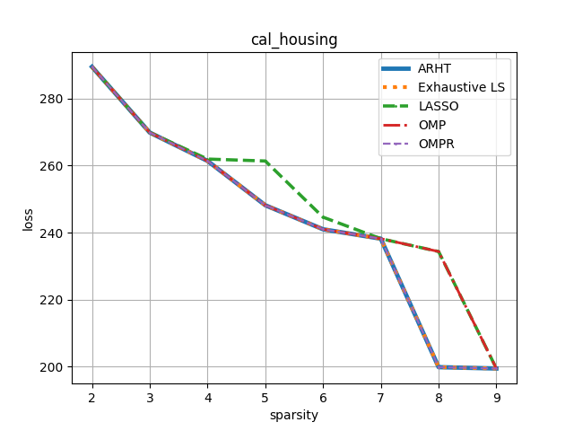
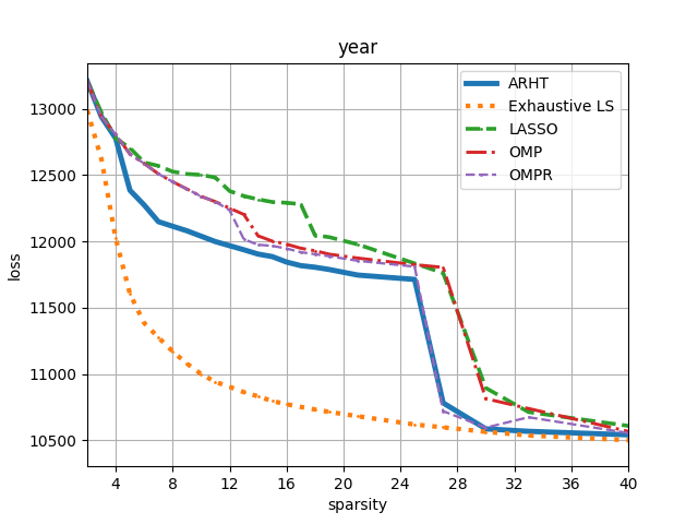
Figure 1: Comparison of different algorithms in the Regression datasets cal_housing and year using the Linear Regression loss.

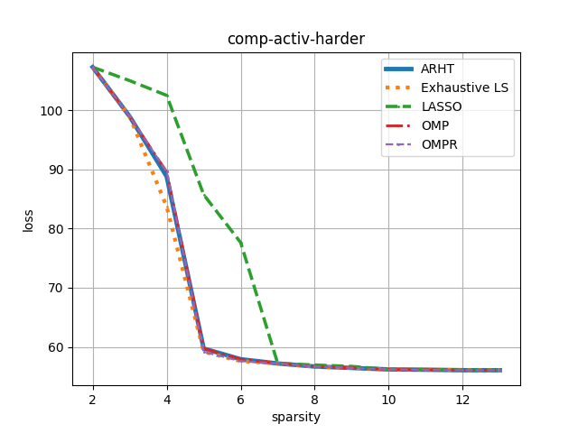
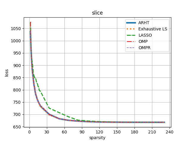
Figure 2: Comparison of different algorithms in the Regression datasets comp-activ-harder and slice using the Linear Regression loss.

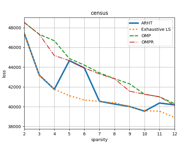
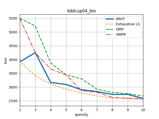
Figure 3: Comparison of different algorithms in the Binary classification datasets census and kddcup04_bio using the Logistic Regression loss.

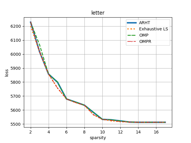
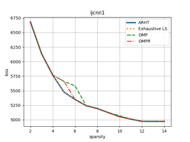
Figure 4: Comparison of different algorithms in the Binary classification datasets letter and ijcnn1 using the Logistic Regression loss.

For experimental evaluation we used well known and publicly available datasets. Their names and basic properties are outlined in Table 2.

Table 2: Datasets used for experimental evaluation. The columns are the dataset name, the number of examples $m$, and the number of features $n$. The datasets can be downloaded here.

Name	$n$	$d$	problem
kddcup04_bio	145750	74	binary
cal_housing	20639	8	regression
census	299284	401	binary
comp-activ-harder	8191	12	regression
ijcnn1	24995	22	binary
letter	20000	16	binary
slice	53500	384	regression
year	463715	90	regression

6.2 Setup details

6.2.1 Basic Definitions

The two quantities that take part in our experiments are the sparsity and the loss of a particular solution. We have already defined and discussed the former at length. The latter refers to the training loss for the problems of Linear Regression and Logistic Regression. We let $m$ denote the number of examples and $n$ the number of features in each example.

In the Linear Regression task we are given the dataset $(A,b)$, where $A\in\mathbb{R}^{m\times n}$, $b\in\mathbb{R}^{m}$. The columns of $A$ correspond to features and the rows to examples. The ($\ell_{2}$ Linear Regression) loss of a solution $x\in\mathbb{R}^{n}$ is defined as $\mathrm{\ell_{2}\_loss}(x)=\frac{1}{2}\left\|Ax-b\right\|_{2}^{2}$.

In the Logistic Regression task we are given the dataset $(A,b)$, where $A\in\mathbb{R}^{m\times n}$, $b\in\{0,1\}^{m}$. The columns of $A$ correspond to features and the rows to examples. The (Logistic Regression) loss of a solution $x\in\mathbb{R}^{n}$ is defined as $\mathrm{logistic\_loss}(x)=\sum\limits_{i\in[m]}\left(-b_{i}\log\sigma(Ax)_{i}-(1-b_{i})\log(1-\sigma(Ax)_{i})\right)$, where $\sigma:\mathbb{R}\rightarrow\mathbb{R}$ defined as $\sigma(t)=\frac{1}{1+e^{-t}}$ is the sigmoid function.

6.2.2 Data Pre-processing

We apply a very basic form of pre-processing to the data. More specifically, we use one-hot encoding to turn categorical features into numerical ones. Then, we discard any examples with missing data so that all the entries of $A$ are defined. We also augment the matrix $A$ with an extra all-ones column (i.e. $\vec{1}$) in order to encode the constant ($y$-intercept) term into $A$, and we scale all the columns of $A$ so that their $\ell_{2}$ norm is $1$. Finally, for the case of ARHT we further augment $A$ in order to encode the regularizer as well. We do this by adding an identity matrix as extra rows. In other words, $A\leftarrow\begin{pmatrix}A\\ I\end{pmatrix}$ and $b\leftarrow\begin{pmatrix}b\\ \vec{0}\end{pmatrix}$.

6.3 Implementation details

The code has been implemented in python3, with libraries numpy, sklearn, and scipy.

6.3.1 Inner Optimization Problem

All the algorithms except for LASSO rely on an inner optimization routine in a restricted subset of coordinates in each step. The inner optimization problem consists of solving a standard Linear Regression or Logistic Regression problem using only a submatrix of $A$ defined by a subset of $s$ of its columns. For that, we use LinearRegression and LogisticRegression from sklearn.linear_model. For Logistic Regression we used an LBFGS solver with $1000$ iterations.

6.3.2 Overall Algorithm

The LASSO solver we used is Lasso from sklearn.linear_model with $1000$ iterations. As LASSO is not tuned in terms of a required sparsity $s$, but rather in terms of the regularization parameter $\alpha$, for each sparsity level we applied binary search on $\alpha$ in order to find a parameter $\alpha$ that gives the required sparsity.

For ARHT, we used a fixed number of $20$ iterations at Line 5 of Algorithm 6. In Line 19 of Algorithm 5 we slightly weaken the progress condition to

$$g_{R^{t}}(x^{t})-g_{R^{t}}(x^{t+1})\geq\frac{10^{-3}}{s}\left(g_{R^{t}}(x^{t})-\mathrm{opt}\right)$$ (17)

so that it does not depend Furthermore, we do not perform a fixed number of iterations. Instead, we use a stopping criterion: If the progress condition (17) is not met and at least half the elements in $x^{t}$ have already been unregularized, i.e. $\left|S^{t}\backslash R^{t}\right|\geq\frac{1}{2}\left|S^{t}\right|$, then we stop. If a desirable solution has not been found, it means that this might be an unsuccessful run, and early termination can be used to detect such runs early and re-start, thus improving the runtime. The routine which samples an index $i$ proportional to $x_{i}^{2}$ was implementing by a standard sampling method that uses binary search on $i$ and flips a random coin at each step. This requires computation of interval sums of $x_{i}^{2}$, which is done by computing partial sums.

Appendix A Deferred Proofs

A.1 Proof of Lemma 3.8

Proof.

$\Phi^{t}$ is a quadratic restricted on $R^{t}$

$$\Phi(y)-\Phi(x)-\nabla\Phi(x)^{T}(y-x)$$

$$=\frac{\rho_{2}^{+}}{2}\left(\left\|y_{R^{t}}\right\|_{2}^{2}-\left\|x_{R^{t}}\right\|_{2}^{2}-2x_{R^{t}}^{T}(y_{R^{t}}-x_{R^{t}})\right)$$

$$=\frac{\rho_{2}^{+}}{2}\left\|y_{R^{t}}-x_{R^{t}}\right\|_{2}^{2}$$

$$\in\left[0,\frac{\rho_{2}^{+}}{2}\left\|y-x\right\|_{2}^{2}\right]$$

and so for any $x,y$ with $|\mathrm{supp}(y-x)|\leq s+s^{*}$ (resp. $|\mathrm{supp}(y-x)|\leq 1$) we have

$$g(y)-g(x)-\nabla g(x)^{T}(y-x)$$

$$=f(y)-f(x)-\nabla f(x)^{T}(y-x)+\Phi(y)-\Phi(x)-\nabla\Phi(x)^{T}(y-x)$$

$$\geq\frac{\rho_{s+s^{*}}^{-}}{2}\left\|y-x\right\|_{2}^{2}\text{(resp.}\leq\rho_{2}^{+}\left\|y-x\right\|_{2}^{2}\text{)}$$

∎

A.2 Proof of Lemma 3.3

Proof.

By definition, and setting $\tau=\frac{1}{s}$, for each Type 1 iteration we have

$$g(x^{t})-g(x^{t+1})\geq\tau\left(g(x^{t})-f(x^{*})\right)$$

$$\Rightarrow g(x^{t+1})-f(x^{*})\leq(1-\tau)(g(x^{t})-f(x^{*}))$$

and in each Type 2 iteration we have

$$g(x^{t+1})-f(x^{*})\leq g(x^{t})-f(x^{*})$$

(since $g$ can only decrease when unregularizing), therefore

$$f(x^{T})-f(x^{*}) \leq g(x^{T})-f(x^{*})$$

$$\leq(1-\tau)^{T_{1}}(g(x^{0})-f(x^{*}))$$

$$\leq e^{-\tau T_{1}}(g(x^{0})-f(x^{*}))$$

$$\leq\epsilon$$

where we used the fact that $T_{1}=\frac{1}{\tau}\log\frac{g(x^{0})-f(x^{*})}{\epsilon}$. ∎

A.3 Proof of Lemma 4.1

Proof.

We have

$$\left(\sqrt{f(x^{t})-f(\widetilde{x}^{t})}+\sqrt{f(x^{*})-f(\widetilde{x}^{t})}\right)^{2} \geq\frac{\rho^{-}}{2}\left(\left\|x^{t}-\widetilde{x}^{t}\right\|_{2}+\left\|x^{*}-\widetilde{x}^{t}\right\|_{2}\right)^{2}$$

$$\geq\frac{\rho^{-}}{2}\left\|x^{t}-x^{*}\right\|_{2}^{2}$$

$$\geq\frac{\rho^{-}}{2}\left(\left\|x^{*}_{S^{*}\backslash S^{t}}\right\|_{2}^{2}+\left\|x_{S^{t}\backslash S^{*}}^{t}\right\|_{2}^{2}\right)$$

where the first inequality follows by applying strong convexity to lower bound $f(x^{t})-f(\widetilde{x}^{t})$ and $f(x^{*})-f(\widetilde{x}^{t})$ combined with the fact that by definition of $\widetilde{x}^{t}$, $\nabla_{S^{t}\cup S^{*}}f(\widetilde{x}^{t})=\vec{0}$, and the second is a triangle inequality. ∎

References

- [ABF+16] Jason Altschuler, Aditya Bhaskara, Gang Fu, Vahab Mirrokni, Afshin Rostamizadeh, and Morteza Zadimoghaddam. Greedy column subset selection: New bounds and distributed algorithms. In International Conference on Machine Learning, pages 2539–2548, 2016.
- [AS14] Joel Andersson and Jan-Olov Strömberg. On the theorem of uniform recovery of random sampling matrices. IEEE Transactions on Information Theory, 60(3):1700–1710, 2014.
- [BCKV15] Holger Boche, Robert Calderbank, Gitta Kutyniok, and Jan Vybíral. A survey of compressed sensing. In Compressed sensing and its applications, pages 1–39. Springer, 2015.
- [BD07] Thomas Blumensath and Mike E Davies. On the difference between orthogonal matching pursuit and orthogonal least squares. 2007.
- [BD09] Thomas Blumensath and Mike E Davies. Iterative hard thresholding for compressed sensing. Applied and computational harmonic analysis, 27(3):265–274, 2009.
- [BRB13] Sohail Bahmani, Bhiksha Raj, and Petros T Boufounos. Greedy sparsity-constrained optimization. Journal of Machine Learning Research, 14(Mar):807–841, 2013.
- [Can08] Emmanuel J Candes. The restricted isometry property and its implications for compressed sensing. Comptes rendus mathematique, 346(9-10):589–592, 2008.
- [CFK18] Lin Chen, Moran Feldman, and Amin Karbasi. Weakly submodular maximization beyond cardinality constraints: Does randomization help greedy? In International Conference on Machine Learning, pages 804–813, 2018.
- [CL06] Fan Chung and Linyuan Lu. Concentration inequalities and martingale inequalities: a survey. Internet Mathematics, 3(1):79–127, 2006.
- [CRT06] Emmanuel J Candes, Justin K Romberg, and Terence Tao. Stable signal recovery from incomplete and inaccurate measurements. Communications on Pure and Applied Mathematics: A Journal Issued by the Courant Institute of Mathematical Sciences, 59(8):1207–1223, 2006.
- [CT05] Emmanuel J Candes and Terence Tao. Decoding by linear programming. IEEE transactions on information theory, 51(12):4203–4215, 2005.
- [CWX09] T Tony Cai, Lie Wang, and Guangwu Xu. Shifting inequality and recovery of sparse signals. IEEE Transactions on Signal processing, 58(3):1300–1308, 2009.
- [CWX10] T Tony Cai, Lie Wang, and Guangwu Xu. New bounds for restricted isometry constants. IEEE Transactions on Information Theory, 56(9):4388–4394, 2010.
- [DMM09] David L Donoho, Arian Maleki, and Andrea Montanari. Message-passing algorithms for compressed sensing. Proceedings of the National Academy of Sciences, 106(45):18914–18919, 2009.
- [Don06] David L Donoho. Compressed sensing. IEEE Transactions on information theory, 52(4):1289–1306, 2006.
- [EDFK17] Ethan Elenberg, Alexandros G Dimakis, Moran Feldman, and Amin Karbasi. Streaming weak submodularity: Interpreting neural networks on the fly. In Advances in Neural Information Processing Systems, pages 4044–4054, 2017.
- [FKT15] Dean Foster, Howard Karloff, and Justin Thaler. Variable selection is hard. In Conference on Learning Theory, pages 696–709, 2015.
- [FL09] Simon Foucart and Ming-Jun Lai. Sparsest solutions of underdetermined linear systems via lq-minimization for 0¡ q¡= 1. Applied and Computational Harmonic Analysis, 26(3):395–407, 2009.
- [Fou10] Simon Foucart. A note on guaranteed sparse recovery via l1-minimization. Applied and Computational Harmonic Analysis, 29(1):97–103, 2010.
- [Fou11] Simon Foucart. Hard thresholding pursuit: an algorithm for compressive sensing. SIAM Journal on Numerical Analysis, 49(6):2543–2563, 2011.
- [Fou12] Simon Foucart. Sparse recovery algorithms: sufficient conditions in terms of restricted isometry constants. In Approximation Theory XIII: San Antonio 2010, pages 65–77. Springer, 2012.
- [FR17] Simon Foucart and Holger Rauhut. A mathematical introduction to compressive sensing. Bull. Am. Math, 54:151–165, 2017.
- [JTD11] Prateek Jain, Ambuj Tewari, and Inderjit S Dhillon. Orthogonal matching pursuit with replacement. In Advances in neural information processing systems, pages 1215–1223, 2011.
- [JTD17] Prateek Jain, Ambuj Tewari, and Inderjit S Dhillon. Partial hard thresholding. IEEE Transactions on Information Theory, 63(5):3029–3038, 2017.
- [JTK14] Prateek Jain, Ambuj Tewari, and Purushottam Kar. On iterative hard thresholding methods for high-dimensional m-estimation. In Advances in Neural Information Processing Systems, pages 685–693, 2014.
- [LYF14] Ji Liu, Jieping Ye, and Ryohei Fujimaki. Forward-backward greedy algorithms for general convex smooth functions over a cardinality constraint. In International Conference on Machine Learning, pages 503–511, 2014.
- [ML11] Qun Mo and Song Li. New bounds on the restricted isometry constant 2k. Applied and Computational Harmonic Analysis, 31(3):460–468, 2011.
- [MTA19] Seyedahmad Mousavi, Mohammad Mehdi Rezaee Taghiabadi, and Ramin Ayanzadeh. A survey on compressive sensing: Classical results and recent advancements. arXiv preprint arXiv:1908.01014, 2019.
- [Nat95] Balas Kausik Natarajan. Sparse approximate solutions to linear systems. SIAM journal on computing, 24(2):227–234, 1995.
- [NT09] Deanna Needell and Joel A Tropp. Cosamp: Iterative signal recovery from incomplete and inaccurate samples. Applied and computational harmonic analysis, 26(3):301–321, 2009.
- [NV09] Deanna Needell and Roman Vershynin. Uniform uncertainty principle and signal recovery via regularized orthogonal matching pursuit. Foundations of computational mathematics, 9(3):317–334, 2009.
- [NV10] Deanna Needell and Roman Vershynin. Signal recovery from incomplete and inaccurate measurements via regularized orthogonal matching pursuit. IEEE Journal of selected topics in signal processing, 4(2):310–316, 2010.
- [SGJN18] Raghav Somani, Chirag Gupta, Prateek Jain, and Praneeth Netrapalli. Support recovery for orthogonal matching pursuit: upper and lower bounds. In Advances in Neural Information Processing Systems, pages 10814–10824, 2018.
- [SL17a] Jie Shen and Ping Li. On the iteration complexity of support recovery via hard thresholding pursuit. In Proceedings of the 34th International Conference on Machine Learning-Volume 70, pages 3115–3124. JMLR. org, 2017.
- [SL17b] Jie Shen and Ping Li. Partial hard thresholding: Towards a principled analysis of support recovery. In Advances in Neural Information Processing Systems, pages 3124–3134, 2017.
- [SSSZ10] Shai Shalev-Shwartz, Nathan Srebro, and Tong Zhang. Trading accuracy for sparsity in optimization problems with sparsity constraints. SIAM Journal on Optimization, 20(6):2807–2832, 2010.
- [Tib96] Robert Tibshirani. Regression shrinkage and selection via the lasso. Journal of the Royal Statistical Society: Series B (Methodological), 58(1):267–288, 1996.
- [YLZ16] Xiaotong Yuan, Ping Li, and Tong Zhang. Exact recovery of hard thresholding pursuit. In Advances in Neural Information Processing Systems, pages 3558–3566, 2016.
- [Zha11] Tong Zhang. Sparse recovery with orthogonal matching pursuit under rip. IEEE Transactions on Information Theory, 57(9):6215–6221, 2011.
- [ZMW+17] Le Zheng, Arian Maleki, Haolei Weng, Xiaodong Wang, and Teng Long. Does -minimization outperform -minimization? IEEE Transactions on Information Theory, 63(11):6896–6935, 2017.