Practical Trade-Offs for the Prefix-Sum Problem

Abstract.

Given an integer array $A$, the prefix-sum problem is to answer $\mbox{{sum}}(i)$ queries that return the sum of the elements in $A[0..i]$, knowing that the integers in $A$ can be changed. It is a classic problem in data structure design with a wide range of applications in computing from coding to databases.

In this work, we propose and compare several and practical solutions to this problem, showing that new trade-offs between the performance of queries and updates can be achieved on modern hardware.

1. Introduction

The prefix-sum problem is defined as follows. Given an array $A[0..n)$ of integers and an index $0\leq i<n$, we are asked to support the following three operations as efficiently as possible.

• $\mbox{{sum}}(i)$ returns the quantity $\sum_{k=0}^{i}A[k]$.

• $\mbox{{update}}(i,\Delta)$ sets $A[i]$ to $A[i]+\Delta$, where $\Delta$ is a quantity that fits in $\delta$ bits.

• $\mbox{{access}}(i)$ returns $A[i]$.

(Note that $\mbox{{access}}(i)$ can be computed as $\mbox{{sum}}(i)-\mbox{{sum}}(i-1)$ for $i>0$ and $\mbox{{access}}(0)=\mbox{{sum}}(0)$. Therefore, we do not consider this operation in the following. Also, a range-sum query $\mbox{{sum}}(i,j)$, asking for the sum of the elements in $A[i..j]$, is computed as $\mbox{{sum}}(j)-\mbox{{sum}}(i-1)$.)

It is an icon problem in data structure design and has been studied rather extensively from a theoretical point of view (Fredman and Saks, 1989; Yao, 1985; Hampapuram and Fredman, 1998; Dietz, 1989; Raman et al., 2001; Hon et al., 2011; Pătraşcu and Demaine, 2006; Chan and Pătraşcu, 2010; Bille et al., 2018, 2017) given its applicability to many areas of computing, such as coding, databases, parallel programming, dynamic data structures and others (Blelloch, 1990). For example, one of the most notable practical applications of this problem is for on-line analytical processing (OLAP) in databases. An OLAP system relies on the popular data cube model (Gray et al., 1997), where the data is represented as a $d$-dimensional array. To answer an aggregate query on the data cube, a prefix-sum query is formulated (see the book edited by Goodman et al. (2017) – Chapter 40, Range Searching by P.K. Agarwal).

Scope of this Work and Overview of Solutions

Despite the many theoretical results, that we review in Section 2, literature about the prefix-sum problem lacks a thorough experimental investigation which is our concern with this work. We aim at determining the fastest single-core solution using commodity hardware and software, that is, a recent manufactured processor with commodity architectural features (such as pipelined instructions, branch prediction, cache hierarchy, and SIMD instructions (Corporation, 2020)), executing C++ compiled with a recent optimizing compiler. (We do not take into account parallel algorithms here, nor solutions devised for specialized/dedicated hardware that would limit the usability of our software. We will better describe our experimental setup in Section 3.)

As a warm-up, let us now consider two trivial solutions to the problem that will help reasoning about the different trade-offs. A first option is to leave $A$ as given. It follows that queries are supported in $O(n)$ by scanning the array and updates take $O(1)$ time. Otherwise, we can pre-compute the result of $\mbox{{sum}}(i)$ and save it in $A[i]$, for every $i$. Then, we have queries supported in $O(1)$, but updates in $O(n)$. These two solutions represent opposite extreme cases: the first achieving fastest update but slowest sum, the second achieving fastest sum but slowest update. (They coincide only when $n$ is bounded by a constant.) However, it is desirable to have a balance between the running times of sum and update. One such trade-off can be obtained by tree-shaped data structures, whose analysis is the scope of our paper.

An elegant solution is to superimpose on $A$ a balanced binary tree. The leaves of the tree store the elements of $A$, whereas the internal nodes store the sum of the elements of $A$ descending from the left and right sub-trees. As the tree is balanced and has height $\lceil\log_{2}n\rceil+1$, it follows that both sum and update translate into tree traversals with $O(1)$ spent per level. This data structure – called Segment-Tree (Bentley, 1977) – guarantees $O(\log n)$ for both queries and updates. Another tree layout having $O(\log n)$-complexity is the Fenwick-Tree (Fenwick, 1994). Differently from the Segment-Tree, the Fenwick-Tree is an implicit data structure, i.e., it consumes exactly $n+1$ memory words for representing $A$ is some appropriate manner. It is not a binary tree and exploits bit-level programming tricks to traverse the implicit tree structure.

Interestingly, it turns out that a logarithmic complexity is optimal for the problem when $\delta$ is as large as the machine word (Pătraşcu and Demaine, 2006). Thus, it is interesting to design efficient implementations of both Segment-Tree and Fenwick-Tree to understand what can be achieved in practice.

Furthermore, it is natural to generalize the Segment-Tree to become $b$-ary and have a height of $\lceil\log_{b}n\rceil$, with $b>2$: an internal node stores an array $B$ of $b-1$ values, where $B[i]$ is the sum of the elements of $A$ covered by the sub-tree rooted in its $i$-th child. Now, we are concerned with solving a smaller instance of the original problem, i.e., the one having $B$ as input array. According to the solution adopted for the “small array”, different complexities can be achieved. To give an idea, one could just adopt one of the two trivial solutions discussed above. If we leave the elements of $B$ as they are, then we obtain updates in $O(\log_{b}n)$ and queries in $O(b\log_{b}n)$. Conversely, if we pre-compute the answers to sum, we have $O(b\log_{b}n)$ for updates and $O(\log_{b}n)$ for queries.

As a matter of fact, essentially all theoretical constructions are variations of a $b$-ary Segment-Tree (Dietz, 1989; Raman et al., 2001; Hon et al., 2011; Pătraşcu and Demaine, 2006). An efficient implementation of such data structure is, therefore, not only interesting for this reason but also particularly appealing in practice because it opens the possibility of using SIMD instructions to process in parallel the $b$ keys stored at each node of the tree. Lastly, also the Fenwick-Tree extends to branching factors larger than 2, but is a less obvious way that we discuss later in the paper.

Contributions

For all the reasons discussed above, we describe efficient implementations of and compare the following solutions: the Segment-Tree, the Fenwick-Tree, the $b$-ary Segment-Tree, and the $b$-ary Fenwick-Tree – plus other optimized variants that we will introduce in the rest of the paper. We show that, by taking into account (1) branch-free code execution, (2) cache-friendly node layouts, (3) SIMD instructions, and (4) compile-time optimizations, new interesting trade-offs can be established on modern hardware.

After a careful experimental analysis, we arrive at the conclusion that an optimized $b$-ary Segment-Tree is the best data structure. Very importantly, we remark that optimizing the Segment-Tree is not only relevant for the prefix-sum problem, because this data structure can also be used to solve several other problems in computational geometry, such as range-min/max queries, rectangle intersection, point location, and three-sided queries. (See the book by de Berg et al. (2008) and references therein for an introduction to such problems.) Thus, the contents of this paper can be adapted to solve these problems as well.

To better support our exposition, we directly show (almost) full C++ implementations of the data structures, in order to guide the reader into a deep performance tuning of the software. We made our best to guarantee that the presented code results compact and easy to understand but without, for any reason, sacrificing its efficiency.

The whole code used in the article is freely available at https://github.com/jermp/psds, with detailed instructions on how to run the benchmarks and reproduce the results.

2. Related Work

Literature about the prefix-sum problem is rich of theoretical results that we summarize here. These results are valid under a RAM model with word size $w$ bits. Let us denote with $t_{q}$ and $t_{u}$ the worst-case complexities for queries and updates respectively.

The first important result was given by Fredman and Saks (1989), who proved a lower bound of $\Omega(\log n/\log w)$, which is $\Omega(\log n/\log\log n)$ for the typical case where an integer fits in one word, i.e., $w=\Theta(\log n)$. They also gave the trade-off $t_{q}\log_{2}(wt_{u})=\Omega(\log n)$. The same lower bound was found by Yao (1985) using a different method. Hampapuram and Fredman (1998) gave a $\Omega(\log n)$ lower bound for the amortized complexity. Dietz (1989) proposed a data structure that achieves Fredman and Saks (1989)’s lower bound for both operations. However, his solution requires $\delta$ to be $O(\log\log n)$ (we recall that $\delta$ is the number of bits needed to represent $\Delta$). He designed a way to handle $b=O(\log^{\varepsilon}n)$ elements in constant time, for some $\varepsilon>0$, and then built a Segment-Tree with branching factor $b$. Thus, the height of the tree is $O(\log_{b}n)=O(\log n/\log\log n)$. To handle $b$ elements in constant time, the prefix sums are computed into an array $B$, whereas the most recent updates are stored into another array $C$. Such array $C$ is handled in constant time using a precomputed table. This solution has been improved by Raman et al. (2001) and then, again, by Hon et al. (2011). The downside of these solutions is that they require large universal tables which do not scale well with $\delta$ and $b$.

Pătraşcu and Demaine (2006) considerably improved the previous lower bounds and trade-off lower bounds for the problem. In particular, they determined a parametric lower bound in $w$ and $\delta$. Therefore, they distinguished two cases for the problem: the case where $\delta=\Omega(w)$ bits and the case where $\delta=o(w)$ bits.

In the former case they found the usual logarithmic bound $\max\{t_{q},t_{u}\}=\Omega(\log n)$. They also found two symmetrical trade-off lower bounds: $t_{q}\log_{2}(t_{u}/t_{q})=\Omega(\log n)$ and $t_{u}\log_{2}(t_{q}/t_{u})=\Omega(\log n)$. This proves the optimality of the Segment-Tree and Fenwick-Tree data structures introduced in Section 1.

In the latter case they found a trade-off lower bound of $t_{q}(\log_{2}(w/\delta)+\log_{2}(t_{u}/t_{q}))=\Omega(\log n)$ which implies the lower bound $\max\{t_{q},t_{u}\}=\Omega(\log n/\log(w/\delta))$. (Note that in the case where $\delta=\Theta(\log n)$ it matches the lower bounds for the first case.) They also proposed a data structure for this latter case that achieves $t_{q}=t_{u}=O(\log n/\log(w/\delta))$ which is optimal for the given lower bound. Their idea is to support both operations in constant time on $b$ elements and build a Segment-Tree with branching factor $b$, as already done by Dietz. Again, the prefix sums for all the elements are precomputed and stored in an array $B$. The recent updates are kept in another array $C$. In particular, and differently from Dietz’s solution, the array $C$ is packed in $w$ bits in order to manipulate it in constant time, which is possible as long as $b=O(w/(\delta+\log w))$.

In Section 7 we will design an efficient and practical implementation of a $b$-ary Segment-Tree, which also takes advantage of smaller bit-widths $\delta$ to enhance the runtime.

The lower bounds found by Pătraşcu and Demaine (2006) do not prevent one of the two operations to be implemented in time $o(\log n)$. Indeed, Chan and Pătraşcu (2010) proposed a data structure that achieves $t_{q}=O(\log n/\log\log n)$ but $t_{u}=O(\log^{0.5+\varepsilon}n)$, for some $\varepsilon>0$. Their idea is (again) to build a Segment-Tree with branching factor $b=\sqrt{w}$. Each node of the tree is represented as another tree, but with branching factor $b^{\prime}=\varepsilon\log w$. This smaller tree supports sum in $O(b/b^{\prime})$ time and update in $O(1+2^{b^{\prime}}b^{2}/w)$ amortized time. To obtain this amortized bound, each smaller tree keeps an extra machine word that holds the $k=w/b$ most recent updates. Every $k$ updates, the values are propagated to the children of the node.

Some Remarks

First, it is important to keep in mind that a theoretical solution may be too complex and, hence, of little practical use, as the constants hidden in the asymptotic bounds are high. For example, we tried to implement the data structure proposed by Chan and Pătraşcu (2010), but soon found out that the algorithm for update was too complicated and actually performed much worse than a simple $O(\log n)$-time solution.

Second, some studies tackle the problem of reducing the space of the data structures (Raman et al., 2001; Hon et al., 2011; Bille et al., 2017; Marchini and Vigna, 2020); in this article we do not take into account compressed representations.

Third, a different line of research studied the problem in the parallel-computing setting where the solution is computed using $p>1$ processors (Meijer and Akl, 1987; Goodrich et al., 1994) or using specialized/dedicated hardware (Harris et al., 2007; Brodnik et al., 2006). As already mentioned in Section 1, we entirely focus on single-core solutions that should run on commodity hardware.

Lastly, several extensions to the problem exist, such as the so-called searchable prefix-sum problem (Raman et al., 2001; Hon et al., 2011), where we are also asked to support the operation $\mbox{{search}}(x)$ which returns the smallest $i$ such that $\mbox{{sum}}(i)\geq x$; and the dynamic prefix-sum problem with insertions/deletions of elements in/from $A$ allowed (Bille et al., 2018).

3. Experimental Setup

Throughout the paper we show experimental results, so we describe here our experimental setup and methodology.

Table 1. Cache hierarchy on the Intel i9-9940X processor. All cache levels have a line size of 64 bytes.

Cache	Associativity	Accessibility	KiB	64-bit Words
$L_{1}$	8	private	32	4,096
$L_{2}$	16	private	1,024	131,072
$L_{3}$	11	shared	19,712	2,523,136

Hardware

For the experiments reported in the article we used an Intel i9-9940X processor, clocked at 3.30 GHz. The processor has two private levels of cache memory per core: $2\times 32$ KiB $L_{1}$ cache (32 KiB for instructions and 32 KiB for data); 1 MiB for $L_{2}$ cache. A $L_{3}$ cache level spans $\approx$19 MiB and is shared among all cores. Table 1 summarizes these specifications. The processor supports the following SIMD (Corporation, 2020) instruction sets: MMX, SSE (including 2, 3, 4.1, 4.2, and SSSE3), AVX, AVX2, and AVX-512.

(We also confirmed our results using another Intel i9-9900X processor, clocked at 3.60 GHz with the same $L_{1}$ configuration, but smaller $L_{2}$ and $L_{3}$ caches. Although timings were slightly different, the same conclusions held.)

Software

All solutions described in the paper were implemented in C++. The code is available at https://github.com/jermp/psds and was tested on Linux with gcc 7.4 and 9.2, and Mac OS with clang 10 and 11. For the experiments reported in the article, the code was compiled with gcc 9.2.1 under Ubuntu 19.10 (Linux kernel 5.3.0, 64 bits), using the flags: -std=c++17 -O3 -march=native -Wall -Wextra.

Methodology

All experiments run on a single core of the processor, with the data residing entirely in memory so that disk operations are of no concern. (The host machine has 128 GiB of RAM.) Performance counts, e.g., number of performed instructions, cycles spent, and cache misses, were collected for all algorithms, using the Linux perf utility. We will use such performance counts in our discussions to further explain the behavior of the algorithms.

We operate in the most general setting, i.e., with no specific assumptions on the data: arrays are made of 64-bit signed integers and initialized at random; the $\Delta$ value for an update operation is also a random signed number whose bit-width is 64 unless otherwise specified.

To benchmark the speed of the operations for a given array size $n$, we generate $10^{4}$ (pseudo-) random natural numbers in the interval $[0,n)$ and use these as values of $i$ for both $\mbox{{sum}}(i)$ and $\mbox{{update}}(i,\Delta)$. Since the running time of update does not depend on the specific value of $\Delta$, we set $\Delta=i$ for the updates.

We show the running times for sum and update using plots obtained by varying $n$ from a few hundreds up to one billion integers. In the plots the minimum and maximum timings obtained by varying $n$ draw a “pipe”, with the marked line inside representing the average time. The values on $n$ used are rounded powers of $10^{1/10}\approx 1.25893$: this base was chosen so that data points are evenly spaced when plotted in a logarithmic scale (Khuong and Morin, 2017). All running times are reported in nanoseconds spent per operation (either, nanosec/sum or nanosec/update). Prior to measurement, a warm-up run is executed to fetch the necessary data into the cache.

4. The Segment-Tree

The Segment-Tree data structure was originally proposed by Bentley (1977) in an unpublished manuscript, and later formalized by Bentley and Wood (1980) to solve the so-called batched range problem (given a set of rectangles in the plane and a query point, report all the rectangles where the point lies in).

Given an array $A[0..n)$, the Segment-Tree is a complete balanced binary tree whose leaves correspond to the individual elements of $A$ and the internal nodes hold the sum of the elements of $A$ descending from the left and right sub-trees. The “segment” terminology derives from the fact that each internal node logically covers a segment of the array and holds the sum of the elements in the segment. Therefore, in simplest words, the Segment-Tree is a hierarchy of segments covering the elements of $A$. In fact, the root of the tree covers the entire array, i.e., the segment $[0,n-1]$; its children cover half array each, that is the segments $[0,\lfloor(n-1)/2\rfloor]$ and $[\lfloor(n-1)/2\rfloor+1,n-1]$ respectively, and so on until the $i$-th leaf spans the segment $[i,i]$ which corresponds to $A[i]$. Figure 1a shows a graphical example for an array of size 16.

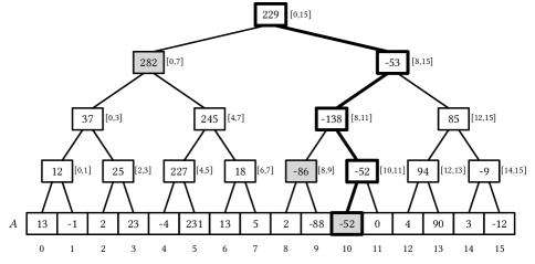
(a)

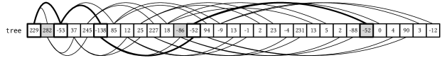
(b)

Figure 1. In (a), an example of Segment-Tree built from an input array $A$, with highlighted nodes belonging to the root-to-leaf path for answering $\mbox{{sum}}(10)$. The shaded nodes are the ones accessed to compute the result, thus $\mbox{{sum}}(10)=282-86-52=144$. In (b), the array-like representation of the same tree.

Top-Down Traversal

Both sum and update can be resolved by traversing the tree structure top-down with a classic binary-search algorithm. For example, Figure 1a highlights the nodes traversed during the computation of $\mbox{{sum}}(10)$. To answer a $\mbox{{sum}}(i)$ query, for every traversed node we determine the segment comprising $i$ by comparing $i$ with the index in the middle of the segment spanned by the node and moving either to the left or right child. Every time we move to the right child, we can sum the value stored in the left child to our result. Updates are implemented in a similar way. Since each child of a node spans half of the segment of its parent, the tree is balanced and its height is $\lceil\log_{2}n\rceil+1$. It follows that sum and update are supported in $O(\log n)$ time.

⬇

struct segment_tree_topdown {

void build(uint64_t const* input, uint64_t n) {

size = 1ULL << uint64_t(ceil(log2(n)));

tree.resize(2 * size - 1, 0);

vector<int64_t> in(size, 0);

copy(input, input + n, in.begin());

visit(in.data(), 0, size - 1, 0);

}

int64_t sum(uint64_t i) const {

uint64_t l = 0, h = size - 1, p = 0;

int64_t sum = 0;

while (l < h) {

if (i == h) break;

uint64_t m = (l + h) / 2;

p = 2 * p + 1;

if (i > m) { sum += tree[p]; l = m + 1; p += 1; }

else h = m;

}

return sum + tree[p];

}

void update(uint64_t i, int64_t delta) {

uint64_t l = 0, h = size - 1, p = 0;

while (l < h) {

tree[p] += delta;

uint64_t m = (l + h) / 2;

p = 2 * p + 1;

if (i > m) { l = m + 1; p += 1; }

else h = m;

}

tree[p] += delta;

}

private:

uint64_t size; vector<int64_t> tree;

int64_t visit(int64_t const* in, uint64_t l, uint64_t h, uint64_t p) {

if (l == h) return tree[p] = in[l];

uint64_t m = (l + h) / 2;

int64_t l_sum = visit(in, l, m, 2 * p + 1);

int64_t r_sum = visit(in, m + 1, h, 2 * p + 2);

return tree[p] = l_sum + r_sum;

}

};

Figure 2. A top-down implementation of the Segment-Tree.

In Figure 2 we give the full code implementing this top-down approach. Some considerations are in order. First, observe that we build the tree by padding the array with zeros until we reach the first power of 2 that is larger-than or equal-to $n$. This substantially simplifies the code, and permits further optimizations that we will introduce later. Second, we store the entire tree in an array, named tree in the code, thus representing the tree topology implicitly with parent-to-child relationships coded via integer arithmetic: if the parent node is stored in the array at position $i$, then its left and right children are placed at positions $2i+1$ and $2i+2$ respectively. Note that this indexing mechanism requires every node of the tree to have two children, and this is (also) the reason why we pad the array with zeros to reach the closest power of two. Figure 1b shows the array-like view of the tree in Figure 1a.

The complete tree hierarchy, excluding the leaves which correspond to the elements of the original array, consists of $2^{\lceil\log_{2}n\rceil}-1$ internal nodes. These internal nodes are stored in the first half of the array, i.e., in tree[0..size-1); the leaves are stored in the second half, i.e., in tree[size-1..2*size-1). Thus the overall Segment-Tree takes a total of $2^{\lceil\log_{2}n\rceil+1}-1$ 64-bit words. Therefore, we have that the Segment-Tree takes $c\cdot n$ memory words, with $c\in[2,4)$. The constant $c$ is 2 when $n$ is a power of 2, but becomes close to 4 when $n$ is very distant from $2^{\lceil\log_{2}n\rceil}$.

Bottom-Up Traversal

In Figure 3 we show an alternative implementation of the Segment-Tree. Albeit logically equivalent to the code shown in Figure 2, this implementation has advantages.

First, it avoids extra space. In particular, it always consumes $2n-1$ memory words, while preserving implicit parent-to-child relationships expressed via integer arithmetic. Achieving this when $n$ is a power of 2 is trivial because the tree will always be full, but is more difficult otherwise. In the build method of the class we show an algorithm that does so. The idea is to let the leaves of the tree, which correspond to the elements of the input, be stored in the array tree slightly out of order. The leaves are still stored in the second half of the array but instead of being laid out consecutively from position n-1 (as it would be if n were a power of 2), they start from position begin, which can be larger than n-1. Let m be $2n-1$. The first m - begin leaves are stored in tree[begin..m); all remaining leaves are stored in tree[n-1,begin). This is achieved with the two for loops in the build method. (Note that begin is always $2^{\lceil\log_{2}n\rceil}-1$ which is $n-1$ if $n$ is a power of 2.) Such circular displacement of the leaves guarantees that parent-to-child relationships are preserved even when $n$ is not a power of 2. Lastly, the visit method traverses the internal nodes recursively, writing in each node the proper sum value.

⬇

struct segment_tree_bottomup {

void build(int64_t const* input, uint64_t n) {

uint64_t m = 2 * n - 1;

tree.resize(m);

size = n;

begin = (1ULL << uint64_t(ceil(log2(n)))) - 1;

uint64_t i = 0, j = 0;

for (; begin + i != m; ++i) tree[begin + i] = input[i];

for (; i != n; ++i, ++j) tree[n - 1 + j] = input[i];

visit(0);

}

int64_t sum(uint64_t i) const {

uint64_t p = leaf(i);

int64_t sum = tree[p];

while (p) {

if ((p & 1) == 0) sum += tree[p - 1]; // p is right child

p = (p - 1) / 2;

}

return sum;

}

void update(uint64_t i, int64_t delta) {

uint64_t p = leaf(i);

while (p) {

tree[p] += delta;

p = (p - 1) / 2;

}

}

private:

uint64_t size, begin; vector<int64_t> tree;

uint64_t leaf(uint64_t i) const {

uint64_t p = begin + i;

p -= (p >= tree.size()) * size;

return p;

}

int64_t visit(uint64_t p) {

if (p >= m_tree.size()) return 0;

if (p >= m_size - 1) return m_tree[p];

int64_t l_sum = visit(2 * p + 1);

int64_t r_sum = visit(2 * p + 2);

return m_tree[p] = l_sum + r_sum;

}

};

Figure 3. A bottom-up implementation of the Segment-Tree.

Second, we now traverse the tree structure bottom-up, instead of top-down. This direction allows a much simpler implementation of the sum and update procedures. The inner while loop is shorter and it is only governed by the index p, which is initialized to be the position of the i-th leaf using the function leaf, and updated to become the index of the parent node at each iteration until it becomes 0, the index of the root node. Furthermore in the code for sum, every time p is the index of a right child we sum the content of its left sibling, which is stored in tree[p-1], to the result.

To check whether p is the index of a right child, we exploit the property that left children are always stored at odd positions in the array; right children at even positions. This can be proved by induction on p. If p is 0, i.e., is the index of the root, then its left child is in position 1 and its right child in position 2, hence the property is satisfied. Now, suppose it holds true when $\mbox{{p}}=k$, for some $k>0$. To show that the property holds for the children of p, it is sufficient to recall that: the double of a number is always even; if we sum 1 to an even number, the result is an odd number (left child); if we sum 2 to an even number, the result is an even number (right child). In conclusion, if the parity of p is 0, it must be a right child. (The parity of p is indicated by its first bit from the right, that we isolate with p & 1.)

Branch-Free Traversal

Whatever implementation of the Segment-Tree we use, either top-down or bottom-up, a branch (if statement) is always executed in the while loop of sum (and in that of update for the top-down variant). For randomly-distributed queries, we expect the branch to be hard to predict: it will be true for approximately half of the times, and false for the others. Using speculative execution as branch-handling policy, the penalty incurred whenever the processor mispredicts a branch is a pipeline flush: all the instructions executed so far (speculatively) must be discarded from the processor pipeline, for a decreased instruction throughput. Therefore, we would like to avoid the branch inside the while loop.

⬇

int64_t sum(uint64_t i) const {

uint64_t n = size;

uint64_t m = (size - 1) / 2, p = 0;

int64_t sum = 0;

while (n != 1) {

uint64_t cmp = i > m;

p = 2 * p + 1;

sum += cmp * tree[p];

p += cmp;

n /= 2;

int64_t offset = cmp * n - n / 2;

m += offset;

}

return sum + tree[p];

}

(a) top-down

⬇

int64_t sum(uint64_t i) const {

uint64_t p = leaf(i);

int64_t sum = tree[p];

while (p) {

uint64_t cmp = (p & 1) == 0;

sum += cmp * tree[p - 1];

p = (p - 1) / 2;

}

return sum;

}

(b) bottom-up

Figure 4. Branch-free sum implementations on the Segment-Tree.

In Figure 4 we show a branch-free implementation of the sum algorithm. It basically uses the result of the comparison, cmp, which will be either 1 or 0, to appropriately mask the quantity we are summing to the result (and move to the proper child obliviously in the top-down traversal). The correctness is immediate and left to the reader. The result of the comparison between the two approaches, branchy vs. branch-free, is shown in Figure 5.

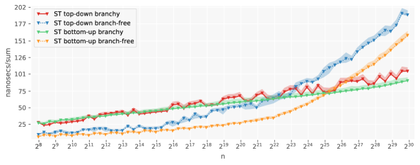
(a) sum

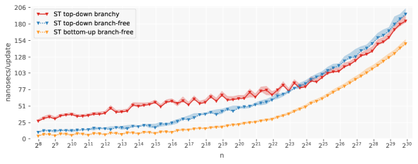
(b) update

Figure 5. Running times for branchy and branch-free sum/update on the Segment-Tree (ST).

As we can see, the branch-free implementations of both sum and update are much faster than the branchy counterparts, on average by $2\times$ or more, for a wide range of practical values of $n$. We collected some performance counts using the Linux perf utility to further explain this evidence. Here we report an example for the bottom-up approach and sum queries. For $n\approx 2^{16}$, the branch-free code spends 66% less cycles than the branchy code although it actually executes 38% more instructions, thus rising the instruction throughput from 0.54 to 2.2. Furthermore, it executes 44% less branches and misses only 0.2% of these. Also, note that the bottom-up version is considerably faster than the top-down version (and does not sacrifice anything for the branchy implementation). Therefore, from now on we focus on the bottom-up version of the Segment-Tree.

However, the branchy implementation of sum is faster than the branch-free one for larger values of $n$ (e.g., for $n>2^{25}$). This shift in the trend is due to the fact that the latency of a memory access dominates the cost of a pipeline flush for large $n$. In fact, when the data structures are sufficiently large, accesses to larger but slower memory levels are involved: in this case, one can obtain faster running times by avoiding such accesses when unnecessary. The branchy implementation does so. In particular, it performs a memory access only if the condition of the branch is satisfied, thus saving roughly 50% of the accesses for a random query workload compared to the branch-free implementation. This is also evident for update. All the different implementations of update perform an access at every iteration of their loop, and this is the reason why all the curves in Figure 5b have a similar shape.

Two-Loop Traversal

In the light of the above considerations, we would actually like to combine the best of the “two worlds” by: executing branch-free code as long as the cost of a pipeline flush exceeds the cost of a memory access, which is the case when the accessed data resides in the smaller cache levels; executing branchy code otherwise, i.e., when the memory latency is the major cost in the running time that happens when the accesses are directed to slower memory levels. Now, the way the Segment-Tree is linearized in the tree array, i.e., the first $n-1$ positions of the array store the internal nodes in level order and the remaining $n$ store the leaves of the tree, is particularly suitable to achieve this. A node at depth $d$ has a $(1/2)^{d}$ probability of being accessed, for randomly distributed queries (root is at depth $d=0$). Therefore when we repeatedly traverse the tree, the first $L_{1}$ positions of the array that correspond to the top-most $\lceil\log_{2}L_{1}\rceil$ levels of the tree are kept in cache $L_{1}$; the following $L_{2}-L_{1}$ positions are kept in $L_{2}$, and so on, where $L_{k}$ indicate the size of the $k$-th cache in data items (the “64-bit Words” column in Table 1 at page 1). If T is the size of the prefix of the array tree that fits in cache, it is intuitive that, as long as $\mbox{{p}}>\mbox{{T}}$, we should prefer the branchy code and save memory accesses; vice versa, when $\mbox{{p}}\leq\mbox{{T}}$, memory accesses are relatively cheap and we should opt for the branch-free code. The following code shows this approach.

⬇

int64_t sum(uint64_t i) const {

uint64_t p = leaf(i);

int64_t sum = tree[p];

while (p > T) {

if ((p & 1) == 0) sum += tree[p - 1]; // branchy

p = (p - 1) / 2;

}

while (p) {

sum += ((p & 1) == 0) * tree[p - 1]; // branch-free

p = (p - 1) / 2;

}

return sum;

}

The value of the threshold T governs the number of loop iterations, out of $\lceil\log_{2}n\rceil+1$, that are executed in a branchy or branch-free manner. Its value intuitively depends on the size of the caches and the value of $n$. For smaller $n$ we would like to set T reasonably high to benefit from the branch-free code; vice versa for larger $n$, we would like to perform more branchy iterations. As a rule-of-thumb, we determined that a good choice of T is $L_{2}-(n>L_{3})\times(L_{2}-L_{1})$, which is equal to $L_{1}$ or $L_{2}$ if $n>L_{3}$ or not respectively.

It remains to explain how we can apply the “two-loop” optimization we have just introduced to the update algorithm, since its current implementation always executes an access per iteration. To reduce the number of accesses to memory, we modify the content of the internal nodes of the tree. If each node stores the sum of the leaves descending from its left subtree only (rather than the sum of the elements covered by the left and right segments), then a memory access is saved every time we do not have to update any node in the left subtree. We refer to this modification of the internal nodes as a left-sum tree hereafter and show the corresponding implementation in Figure 6.

Lastly, Figure 7 illustrates the comparison between branchy/branch-free implementations of regular and left-sum Segment-Tree. As apparent from the plots, the left-sum variant with the two-loop optimization is the fastest Segment-Tree data structure because it combines the benefits of branch-free and branchy implementations. From now on and further comparisons, we simply refer to this strategy as ST in the plots.

⬇

struct segment_tree_bottomup_leftsum {

void build(int64_t const* input, uint64_t n); // same as in Figure 3

int64_t sum(uint64_t i) const {

uint64_t p = leaf(i);

uint64_t T = L2 - (size > L3) * (L2 - L1);

int64_t sum = tree[p];

while (p > T) {

uint64_t parent = (p - 1) / 2;

if ((p & 1) == 0) sum += tree[parent];

p = parent;

}

while (p) {

uint64_t parent = (p - 1) / 2;

sum += ((p & 1) == 0) * tree[parent];

p = parent;

}

return sum;

}

void update(uint64_t i, int64_t delta) {

uint64_t p = leaf(i);

uint64_t T = L2 - (size > L3) * (L2 - L1);

tree[p] += delta;

while (p > T) {

uint64_t parent = (p - 1) / 2;

if ((p & 1) == 1) tree[parent] += delta;

p = parent;

}

while (p) {

uint64_t parent = (p - 1) / 2;

tree[parent] += ((p & 1) == 1) * delta;

p = parent;

}

}

private:

uint64_t size, begin;

vector<int64_t> tree;

uint64_t leaf(uint64_t i) const; // same as in Figure 3

int64_t visit(uint64_t p) {

uint64_t l = 2 * p + 1;

if (l >= tree.size()) return tree[p];

int64_t l_sum = visit(l), r_sum = visit(l + 1);

return (tree[p] = l_sum) + r_sum;

}

};

Figure 6. The bottom-up left-sum Segment-Tree implementation that stores in each internal node the sum of the leaves descending from its left sub-tree.

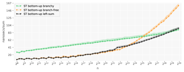
(a) sum

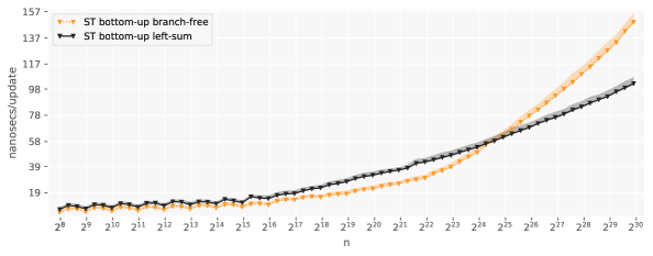
(b) update

Figure 7. Comparison between branchy/branch-free implementations of regular and left-sum Segment-Tree.

5. The Fenwick-Tree

The solution we describe here is popularly known as the Fenwick-Tree (or Binary Indexed Tree, BIT) after a paper by Fenwick (1994), although the underlying principle was introduced by Ryabko (1992).

The key idea is to exploit the fact that, as a natural number $i>0$ can be expressed as sum of proper powers of 2, so sum/update operations can be implemented by considering array locations that are power-of-2 elements apart. For example, since $11=2^{3}+2^{1}+2^{0}=8+2+1$, then $\mbox{{sum}}(10)$ can be computed as $\mbox{{tree}}[2^{3}]+\mbox{{tree}}[2^{3}+2^{1}]+\mbox{{tree}}[2^{3}+2^{1}+2^{0}]=\mbox{{tree}}[8]+\mbox{{tree}}[10]+\mbox{{tree}}[11]$, where the array tree is computed from $A$ in some appropriate manner that we are going to illustrate soon. In this example, $\mbox{{tree}}[8]=\sum_{k=0}^{8-1}A[k]$, $\mbox{{tree}}[10]=A[8]+A[9]$, and $\mbox{{tree}}[11]=A[10]$.

Now, let $\mbox{{base}}=0$. The array $\mbox{{tree}}[0..n+1)$ is obtained from $A$ with the following two-step algorithm.

1. Store in $\mbox{{tree}}[\mbox{{base}}+i]$ the quantity $\sum_{k=0}^{i-1}A[\mbox{{base}}+k]$ where $i=2^{j}$, $j=0,1,2,\ldots$

2. For every sub-array $A[2^{j}..2^{j+1}-1)$, repeat step (1) with updated $\mbox{{base}}=2^{j}$.

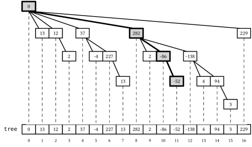
Figure 8. An example of the array-like view tree of the Fenwick-Tree, along with its logical “interrogation” tree. The array tree is built from the input array $[$13, -1, 2, 23, -4, 231, 13, 5, 2, -88, -52, 0, 4, 90, 3, -12$]$. As in Figure 1a, highlighted nodes belong to the root-to-leaf path that is traversed to answer sum for index 10.

Figure 8 shows a tree-like view of one such array tree, built from the same array $A$ of size 16 shown in Figure 1a. Note that position 0 is never used for ease of notation and $\mbox{{tree}}[0]=0$, thus tree’s actual size is $n+1$. Now, we said that during a sum query for index $i$ (or update) we only touch tree’s positions that are power-of-2 elements apart. It is not difficult to see that we have one such position for every bit set in the binary representation of $i$. Since $i$ goes from 0 to $n-1$, it needs $\lceil\log_{2}(n+1)\rceil$ bits to be represented, so this will also be the height of the Fenwick-Tree. (The depth of a node whose index is $i$ is the Hamming weight of $i$, i.e., the number of bits set in the binary representation of $i$.) Therefore, both queries and updates have a worst-case complexity of $O(\log n)$ and the array tree takes $n+1$ memory words. In the following we illustrate how to navigate the implicit tree structure in order to support sum and update.

Let us consider the sum query. As intuitive from the given examples, when we have to answer $\mbox{{sum}}(i)$, we actually probe the array tree starting from index $\mbox{{p}}=i+1$. This is because index 0 is not a power of 2, thus is can be considered as a dummy entry in the array tree. Now, let p be 11 as in the example of Figure 8. The sequence of nodes’ indexes touched during the traversal to compute the result are (bottom-up): $11\rightarrow 10\rightarrow 8\rightarrow 0$. It is easy to see that we always start from index $i+1$ and end with index 0 (the root of the tree). To navigate the tree bottom-up we need an efficient way of computing the index of the parent node from a given index p. This operation can be accomplished by clearing the least significant bit (LSB) of the binary representation of p. For example, 11 is 01011 in binary. We underline its LSB. If we clear the LSB, we get the bit configuration 01010 which indeed corresponds to index 10. Clearing the LSB of 10 gives 01000 which is 8. Finally, clearing the LSB of a power of 2 will always give 0, that is the index of the root. This operation, clearing the LSB of a given number p, can be implemented efficiently with p & (p - 1). Again, note that $\mbox{{sum}}(i)$ traverses a number of nodes equal to the number of bits set (plus 1) in $\mbox{{p}}=i+1$. The code given in Figure 10 illustrates the approach.

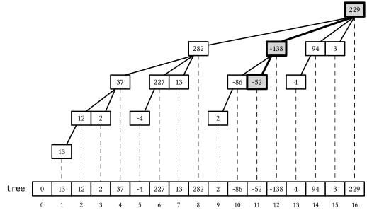
Figure 9. The logical “updating” tree for the same example shown in Figure 8. The highlighted nodes belong to the root-to-leaf path that is traversed to perform update for index 10.

The Fenwick-Tree can be actually viewed as the superimposition of two different trees. One tree is called the “interrogation” tree because it is used during sum, and it is shown in Figure 8. The other tree is called the “updating” tree, and it is shown in Figure 9 instead. This tree consists of the very same nodes as the “interrogation” tree but with different child-to-parent relationships. In fact, starting from an index $\mbox{{p}}=i+1$ and traversing the tree bottom-up we obtain the sequence of nodes that need to be updated when issuing $\mbox{{update}}(i,\Delta)$. Again for the example $i=10$, such sequence is $11\rightarrow 12\rightarrow 16$. Starting from a given index p, this sequence can be obtained by isolating the LSB of p and summing this to p itself. The LSB can be isolated with the operation p & -p. For $\mbox{{update}}(i,\Delta)$, the number of traversed node is equal to the number of leading zeros (plus 1) in the binary representation of $\mbox{{p}}=i+1$. The actual code for update is given in Figure 10.

⬇

struct fenwick_tree {

void build(uint64_t const* input, uint64_t n) {

tree.resize(n + 1, 0);

copy(input, input + n, tree.begin() + 1);

for (uint64_t step = 2; step <= n; step *= 2)

for (uint64_t i = step; i <= n; i += step) tree[i] += tree[i - step / 2];

}

int64_t sum(uint64_t i) const {

int64_t sum = 0;

uint64_t p = i + 1;

while (p) { sum += tree[p]; p &= p - 1; }

return sum;

}

void update(uint64_t i, int64_t delta) {

uint64_t p = i + 1;

while (p < tree.size()) { tree[p] += delta; p += p & -p; }

}

private:

vector<int64_t> tree;

};

Figure 10. The Fenwick-Tree code.

Figure 11. Number of distinct cache lines stored in each set of a $L_{1}$ 8-way set-associative cache, after running $10^{4}$ random sum queries with a Fenwick-Tree of size $n=10^{7}$.

Cache Conflicts

The indexing of the nodes in the Fenwick-Tree – which, for every subtree, places the nodes on the same level at array locations that are power-of-2 elements apart – induces a bad exploitation of the processor cache for large values of $n$. The problem comes from the fact that cache memories are typically $c$-way set-associative caches. The cache memory of the processor used for the experiments in this article is no exception. In such cache architecture, a cache line must be stored in one (and only one) set and, if many different cache lines must be stored in the same set, the set has only room for $c$ of these. In fact, when the set fills up, a cache line must be evicted from the set. If the evicted line is then accessed again during the computation a cache miss will be generated because the line is not in the cache anymore. Therefore, accessing (more than $c$) different memory lines that must be stored in the same cache set will induce cache misses. To understand why this happens in the Fenwick-Tree, let us consider how the set number is determined from a memory address $a$.

Let $C$ be the total cache size in bytes, where each line spans 64 bytes. The cache stores its lines as divided into $C/(c\times 64)$ sets, where each set can store a cache line in $c$ different possible “ways”. For example, the $L_{1}$ cache of the processor used for the experiments in this article (see Table 1 at page 1) has 8 ways and a total of $C=$32,768$$ bytes. Therefore there are $$32,768$/(8\times 64)=64$ sets in the cache, for a total of 512 cache lines. The first 6 bits (0-5) of $a$ determine the offset into the cache line; the following 6 bits (6-11) specify the set number. Thus, the first line of a memory block is stored in the set 0, the second line is stored in set 1, ecc. The 64-th line will be stored again in set 0, the 65-th line in set 1, ecc. It is now easy to see that accessing memory addresses that are multiple of $64\times 64=$4096$$ bytes (a memory page) is not cache efficient, since the lines will contend the very same set.

Therefore, accessing memory locations whose distance in memory is a large power of 2 (multiple of $2^{12}=4096$) is not cache-friendly. Unfortunately, this is what happens in the Fenwick-Tree when $n$ is large. For example, all the nodes at the first level are stored at indexes that are powers of 2. Thus they will all map to the set 0. In Figure 11 we show the number of distinct cache lines that must be stored in each set of the cache $L_{1}$ (8-way set-associative with 64 sets), for $10^{4}$ random sum queries and $n=10^{7}$. For a total of $\approx$4$\times 10^{4}$ cache lines accessed, 29% of these are stored in set 0. This highly skewed distribution is the source of cache inefficiency. (Updates exhibit the same distribution.) Instead, if all accesses were evenly distributed among all sets, we would expect each set to contain $\approx$625 lines (1.56%).

This problem can be solved by inserting some holes in the tree array (Marchini and Vigna, 2020), one every $d$ positions, to let a node whose position is $i$ in the original array to be placed at position $i+\lfloor i/d\rfloor$. This only requires the tree array to be enlarged by $\lfloor n/d\rfloor$ words and to recalculate the index of every node accordingly. If $d$ is chosen to be a sufficiently large constant, e.g., $2^{14}$, then the extra space is very small. In Figure 12 we show the result of the same experiment as in Figure 11, but after the modification to the tree array and the new indexing of the nodes. As it is evident, now every cache set is equally used. (For comparison, we also report the behavior of the Segment-Tree to confirm that also in this case there is a good usage of the cache.)

(a) modified Fenwick-Tree

(b) Segment-Tree

Figure 12. The same experiment as performed in Figure 11, but after reducing the cache conflicts in the Fenwick-Tree (modified). For comparison, we also report the cache usage of the Segment-Tree.

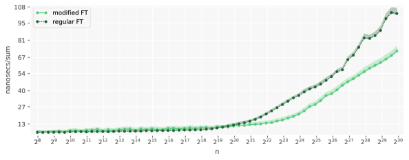
(a) sum

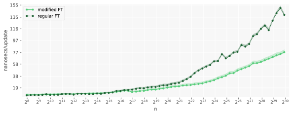
(b) update

Figure 13. The running times of sum/update for the regular and modified Fenwick-Tree (FT).

Lastly, in Figure 13 we show the comparison between the regular Fenwick-Tree and the modified version as described above. As expected, the two curves are very similar up to $n=2^{20}$, then the cache conflicts start to pay a significant role in the behavior of the regular Fenwick-Tree, making the difference between the two curves to widen progressively. As an example, collecting the number of cache misses using Linux perf for $n\approx 250\times 10^{6}$ (excluding those spent during the construction of the data structures and generation of the queries) indeed reveals that the regular version incurs in $2.5\times$ the cache-misses of the modified version, for both sum and update.

From now on, we simply refer to the modified Fenwick-Tree without the problem of cache conflicts as FT in the plots for further comparisons.

6. Segment-Tree vs. Fenwick-Tree

In this section we compare the optimized versions of the the Segment-Tree and Fenwick-Tree – respectively, the bottom-up left-sum Segment-Tree with 2-loop traversal, and the modified Fenwick-Tree with reduced cache conflicts. A quick look at Figure 14 immediately reveals that the Fenwick-Tree outperforms the Segment-Tree. There are two different reasons that explain why the Fenwick-Tree is more efficient than the Segment-Tree.

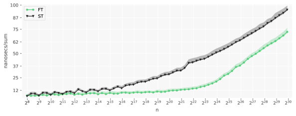
(a) sum

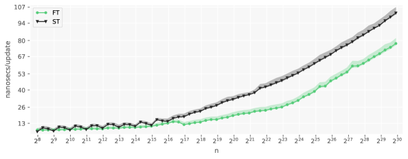
(b) update

Figure 14. The running times of sum/update for the Segment-Tree (ST) and the Fenwick-Tree (FT).

1. Although we have substantially simplified the code logic for traversing the Segment-Tree with the bottom-up navigation, the code for the Fenwick-Tree is even simpler and requires just a few arithmetic operations plus a memory access at each iteration of the loop.

2. While both trees have height $\lceil\log_{2}n\rceil+1$, the number of traversed nodes per operation is different. The Segment-Tree always traverses $\lceil\log_{2}n\rceil+1$ nodes and that is also the number of iterations of the while loop. When the branch-free code is into play, also $\lceil\log_{2}n\rceil+1$ memory accesses are performed. As we already explained, for the branchy implementation the number of memory accesses depends on the query: for random distributed queries we expect to perform one access every two iterations of the loop (i.e., half of the times we go left, half of the time we go right). Now, for a random integer $i$ between 0 and $n-1$, the number of bits set we expect to see in its binary representation is approximately 50%. Therefore, the number of loop iterations and memory accesses the Fenwick-Tree is likely to perform is $\frac{1}{2}\lceil\log_{2}(n+1)\rceil+1$, i.e., half of those performed by the Segment-Tree, regardless the value of $n$.

Both factors contribute to the difference in efficiency between the two data structures. However, for small values of $n$, the number of performed instructions is the major contributor in the running time as both data structures fit in cache, thus memory accesses are relatively cheap (point 1). For example, when $n$ is $\approx 2^{16}$ and considering sum queries, the Fenwick-Tree code spends 58% of the cycles spent by the Segment-Tree and executes nearly 1/3 of instructions. It also executes half of the branches and misses 11% of them. Moving towards larger $n$, the memory latency progressively becomes the dominant factor in the running time, thus favoring solutions that spare memory accesses (point 2). Considering again the number of cache misses for $n\approx 250\times 10^{6}$ (excluding overheads during benchmarking), we determined that the Fenwick-Tree incurs in 25% less cache misses than the Segment-Tree for both sum and update.

In conclusion, we will exclude the Segment-Tree from the experiments we are going to discuss in the rest of the paper and compare against the Fenwick-Tree.

7. The $b$-ary Segment-Tree

The solutions analyzed in the previous sections have two main limitations. (1) The height of the tree is $\lceil\log_{2}n\rceil+1$: for the Segment-Tree, because each internal node has 2 children; for the Fenwick-Tree, because an index in $[0,n)$ is decomposed as sum of some powers of 2. Thus, the tree may become excessively tall for large values of $n$. (2) The running time of update does not depend on $\Delta$. In particular, it makes no difference whether $\Delta$ is “small”, e.g., it fits in one byte, or arbitrary big: possible assumptions on $\Delta$ are not currently exploited to achieve a better runtime.

To address these limitations, we can let each internal node of the tree hold a block of $b>2$ keys. While this reduces the height of the tree for a better cache usage, it also enables the use of SIMD instructions for faster update operations because several keys can be updated in parallel.

Therefore, in Section 7.1 we introduce a solution that works for “small” arrays of $b>2$ keys, e.g., 64 or 256. Then, in Section 7.2, we show how to embed this small-array solution into the nodes of a Segment-Tree to obtain a solution for arbitrary values of $n$.

7.1. Prefix Sums on Small Arrays: SIMD-Aware Node Layouts

⬇

static const uint64_t all1 = uint64_t(-1);

static const uint64_t T[4 * 4] = {

0, all1, all1, all1,

0, 0, all1, all1,

0, 0, 0, all1,

0, 0, 0, 0

};

void update(uint64_t i, int64_t delta) {

__m256i U = _mm256_set1_epi64x(delta);

__m256i msk = _mm256_load_si256((__m256i const*)T + i);

__m256i K = _mm256_loadu_si256((__m256i const*)keys);

U = _mm256_and_si256(U, msk);

_mm256_storeu_si256((__m256i*)keys, _mm256_add_epi64(U, K));

}

Figure 15. A SIMD-based implementation of update for an array keys of 4 $\times$ 64-bit integers. The table T must be aligned on a 32-byte boundary.

A reasonable starting point would be to consider $b=4$ keys and compute their prefix sums in an array $\mbox{{keys}}[0..4)$. Queries are answered in the obvious way: $\mbox{{sum}}(i)=\mbox{{keys}}[i]$, and we do not explicitly mention it anymore in the following. Instead, an $\mbox{{update}}(i,\Delta)$ operation is solved by setting $\mbox{{keys}}[j]=\mbox{{keys}}[j]+\Delta$ for $j=i..3$. We can do this in parallel with SIMD as follows. Let U be a register of $4\times 64$ bits that packs 4 integers, where the first $i-1$ integers are 0 and the remaining ones, from $j=i..3$, are equal to $\Delta$. Then $\mbox{{update}}(i,\Delta)$ is achieved by adding U and keys in parallel using the instruction _mm256_add_epi64. To obtain the register U as desired, we first initialize U with 4 copies of $\Delta$ using the instruction _mm256_set1_epi64x. Now, the copies of $\Delta$ before the $i$-th must be masked out. To do so, we use the index $i$ to perform a lookup into a small pre-computed table T, where $\mbox{{T}}[i]$ is the proper 256-bit mask. In this case, T is a $4\times 4$ table of unsigned 64-bit integers, where $\mbox{{T}}[0][0..3]=[0,2^{64}-1,2^{64}-1,2^{64}-1]$, $\mbox{{T}}[1][0..3]=[0,0,2^{64}-1,2^{64}-1]$, $\mbox{{T}}[2][0..3]=[0,0,0,2^{64}-1]$, and $\mbox{{T}}[3][0..3]=[0,0,0,0]$. Once we loaded the proper mask, we obtain the wanted register configuration with $\mbox{{U}}=\mbox{{\_mm256\_and\_si256}}(\mbox{{U}},\mbox{{T}}[i])$. The code for this algorithm is shown in Figure 15.

An important observation is in order, before proceeding. One could be tempted to leave the integers in $\mbox{{keys}}[0..4)$ as they are in order to obtain trivial updates and use SIMD instructions to answer sum. During our experiments we determined that this solution gives a worse trade-off than the one described above: this was actually no surprise, considering that the algorithm for computing prefix sums with SIMD is complicated as it involves several shifts and additions (besides load and store). Therefore, SIMD is more effective on updates rather than queries.

Two-Level Data Structure

As already motivated, we would like to consider larger values of $b$, e.g., 64 or 256, in order to obtain even flatter trees. Working with such branching factors, would mean to apply the algorithm in Figure 15 for $b/4$ times, which may be too slow. To alleviate this issue, we use a two-level data structure. We split $b$ into $\sqrt{b}$ segments and store each segment in prefix-sum. The sum of the integers in the $j$-th segment is stored in a summary array of $\sqrt{b}$ values in position $j+1$, for $j=0..\sqrt{b}-2$ ($\mbox{{summary}}[0]=0$). The values of the summary are stored in prefix-sum as well. In Figure 16 we show a graphical example of this organization for $b=16$. In the example, we apply the algorithm in Figure 15 only twice (first on the summary, then on a specific segment of keys): without the two-level organization, 4 executions of the algorithm would have been needed. Instead, queries are as easy as $\mbox{{sum}}(i)=\mbox{{summary}}[i/\sqrt{b}]+\mbox{{keys}}[i]$.

The code corresponding to this approach for $b=64$ is shown in Figure 17. In this case, note that the whole summary fits in one cache line, because its size is $8\times 8=64$ bytes, as well as each segment of keys. The table T stores $(8+1)\times 8$ 64-bit unsigned values, where $\mbox{{T}}[i][0..7]$ is a an array of 8 integers: the first $i$ are 0 and the other $8-i$ are $2^{64}-1$, for $i=0..8$.

Lastly, the space overhead due to the summary array is always $1/\sqrt{b}\times 100\%$. For the example code in Figure 17, the space consumed is 12.5% more than that of the input array (576 bytes consumed instead of $64\times 8=512$).

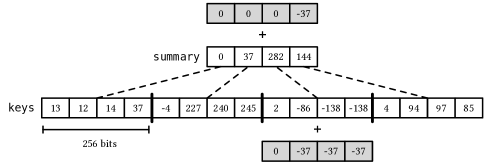
Figure 16. A two-level node layout built from the array $[$13, -1, 2, 23, -4, 231, 13, 5, 2, -88, -52, 0, 4, 90, 3, -12$]$. The shaded arrays represent the content of the registers used when executing the operation $\mbox{{update}}(9,-37)$.

⬇

struct node {

static const uint64_t fanout = 64, size = 576;

node(uint8_t* ptr)

: summary(reinterpret_cast<int64_t*>(ptr))

, keys(reinterpret_cast<int64_t*>(ptr) + 8)

{}

static void build(int64_t const* input, uint8_t* out);

void update(uint64_t i, int64_t delta) {

uint64_t j = i / 8, k = i % 8;

__m256i U = _mm256_set1_epi64x(delta);

__m256i msk_j0 = _mm256_load_si256((__m256i const*)(T + 8) + 2 * j + 0);

__m256i msk_j1 = _mm256_load_si256((__m256i const*)(T + 8) + 2 * j + 1);

__m256i U_j0 = _mm256_and_si256(U, msk_j0);

__m256i U_j1 = _mm256_and_si256(U, msk_j1);

__m256i dst_summary0 = _mm256_loadu_si256((__m256i const*)summary + 0);

__m256i dst_summary1 = _mm256_loadu_si256((__m256i const*)summary + 1);

_mm256_storeu_si256((__m256i*)summary + 0, _mm256_add_epi64(U_j0, dst_summary0));

_mm256_storeu_si256((__m256i*)summary + 1, _mm256_add_epi64(U_j1, dst_summary1));

__m256i msk_k0 = _mm256_load_si256((__m256i const*)T + 2 * k + 0);

__m256i msk_k1 = _mm256_load_si256((__m256i const*)T + 2 * k + 1);

__m256i U_k0 = _mm256_and_si256(U, msk_k0);

__m256i U_k1 = _mm256_and_si256(U, msk_k1);

__m256i dst_keys0 = _mm256_loadu_si256((__m256i const*)(keys + j * 8) + 0);

__m256i dst_keys1 = _mm256_loadu_si256((__m256i const*)(keys + j * 8) + 1);

_mm256_storeu_si256((__m256i*)(keys + j * 8) + 0, _mm256_add_epi64(U_k0, dst_keys0));

_mm256_storeu_si256((__m256i*)(keys + j * 8) + 1, _mm256_add_epi64(U_k1, dst_keys1));

}

int64_t sum(uint64_t i) const { return summary[i / 8] + keys[i]; }

private:

int64_t *summary, *keys;

};

Figure 17. Code for a two-level node data structure with $b=64$.

⬇

struct node {

static const uint64_t fanout = 64, size = 721;

node(uint8_t* ptr)

: summary(reinterpret_cast<int64_t*>(ptr))

, keys(reinterpret_cast<int64_t*>(ptr) + 8)

, summary_buffer(reinterpret_cast<int16_t*>(ptr) + 288)

, keys_buffer(reinterpret_cast<int16_t*>(ptr) + 296)

, updates(ptr + size - 1)

{}

static void build(int64_t const* input, uint8_t* out);

void update(uint64_t i, int8_t delta) {

uint64_t j = i / 8, k = i % 8;

__m128i U = _mm_set1_epi16(delta);

__m128i msk_j = _mm_load_si128((__m128i const*)(T + 8) + j);

__m128i U_j = _mm_and_si128(U, msk_j);

__m128i dst_summary_buffer = _mm_loadu_si128((__m128i const*)summary_buffer);

_mm_storeu_si128((__m128i*)summary_buffer, _mm_add_epi16(U_j, dst_summary_buffer));

__m128i msk_k = _mm_load_si128((__m128i const*)T + k);

__m128i U_k = _mm_and_si128(U, msk_k);

__m128i dst_keys_buffer = _mm_loadu_si128((__m128i const*)keys_buffer + j);

_mm_storeu_si128((__m128i*)keys_buffer + j, _mm_add_epi16(U_k, dst_keys_buffer));

*updates += 1;

if (*updates == 255) {

for (uint64_t l = 0; l != 8; ++l) {

summary[l] += summary_buffer[l];

summary_buffer[l] = 0;

}

for (uint64_t l = 0; l != 64; ++l) {

keys[l] += keys_buffer[l];

keys_buffer[l] = 0;

}

}

}

int64_t sum(uint64_t i) const {

return summary[i / 8] + keys[i] + summary_buffer[i / 8] + keys_buffer[i];

}

private:

int64_t *summary, *keys; int16_t *summary_buffer, *keys_buffer; uint8_t *updates;

};

Figure 18. Code for a two-level node data structure with $b=64$, for the “restricted” case where $\Delta$ is a signed 8-bit integer.

Handling Small Updates

It is intuitive that one can obtain faster results for update if the bit-width of $\Delta$ is smaller than 64. In fact, a restriction on the possible values $\Delta$ can take permits to “pack” more such values inside a SIMD register which, in turn, allows to update a larger number of keys in parallel. As we already observed, neither the binary Segment-Tree nor the Fenwick-Tree can possibly take advantage of this restriction.

To exploit this possibility, we buffer the updates. We restrict the bit-width of $\Delta$ to 8, that is, $\Delta$ is now a value in the range $[-128,+127]$ (instead of the generic, un-restricted, case of $\Delta\in[-2^{63},+2^{63}-1]$). We enrich the two-level node layout introduced before with some additional arrays to buffer the updates. These arrays are made of 16-bit signed integers. We maintain one such array of size $\sqrt{b}$, say summary_buffer, plus another of size $b$, keys_buffer. In particular, the $i$-th value of keys_buffer holds the $\Delta$ value for the $i$-th key; similarly, the $(j+1)$-th value of summary_buffer holds the $\Delta$ value for the $j$-th segment. The buffers are kept in prefix-sum.

Upon an $\mbox{{update}}(i,\Delta)$ operation, the buffer for the summary and that of the specific segment comprising $i$ are updated using SIMD. The key difference now is that – because we work with smaller integers – 8, or even 16, integers are updated simultaneously, instead of only 4 as illustrated with the code in Figure 15.

For example, suppose $b=64$. The whole summary_buffer, which consists of $16\times 8=128$ bits, fits into one SSE SIMD register, thus 8 integers are updated simultaneously. For $b=256$, 16 integers are updated simultaneously because $16\times 16=256$ bits again fit into one AVX SIMD register. This makes a big improvement with respect to the un-restricted case because instead of executing the algorithm in Figure 15 for $\sqrt{b}/4$ times, only one such update is sufficient. This potentially makes the restricted case $2\times$ and $4\times$ faster than the un-restricted case for $b=64$ and $b=256$ respectively.

To avoid overflow issues, we bring the keys (and the summary) up-to-date by reflecting on these the updates stored in the buffer. Since we can perform a maximum of $-2^{15}/-128=256$ updates before overflowing, we clean the buffers every 256 update operations. The solution described here holds, therefore, in the amortized sense.

Figure 18 contains the relevant code illustrating this approach. The code should be read as the “restricted” variant of that shown in Figure 17. We count the number of updates with a single 8-bit unsigned integer, updates, which is initialized to 255 in the build method. When this variable is equal to 255, it will overflow the next time it is incremented by 1, indeed making it equal to 0. Therefore we correctly clean the buffers every 256 updates.

In this case, the table T stores $(16+1)\times 16$ 16-bit unsigned values, where each $\mbox{{T}}[i][0..15]$ contains a prefix of $i$ zeros, followed by $16-i$ copies of $2^{16}-1$, for $i=0..16$.

Also, sum queries are now answered by computing the sum between four quantities, which is actually more expensive than the queries for the general case.

The data structure consumes $(2b+10\sqrt{b}+1)/(8b)\times 100\%$ more bytes than the input. For $b=64$, as in the code given in Figure 18, this extra space is 40.8%; for $b=256$, it is 32.9%.

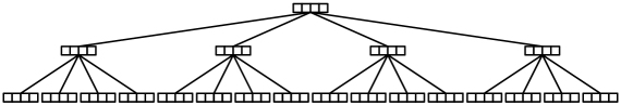
Figure 19. The shape of $b$-ary Segment-Tree with $b=4$, built from an input array of size 64.

7.2. Prefix Sums on Large Arrays

In this section we use the two-level data structures introduced in Section 7.1 in the nodes of a Segment-Tree, to establish new practical trade-offs. If $b$ is the node’s fanout, this solution provides a tree of height $\lceil\log_{b}n\rceil$, whose shape is illustrated in Figure 19 for the case $b=4$ and $n=64$. The code in Figure 20 takes a generic Node structure as a template parameter and builds the tree based on its fanout and size (in bytes). In what follows, we shall first discuss some optimizations and then illustrate the experimental results.

Avoiding Loops and Branches

The tree data structure is serialized in an array of bytes, the tree array in the code. In a separate array, nodes, we keep instead the number of nodes at each level of the tree. This information is used to traverse the tree. In particular, when we have to resolve an operation at a given tree level, all we have to do is to instantiate a Node object at a proper byte location in the array tree and call the desired sum/update method of the object. Such proper byte location depends on both the number of nodes in the previous levels and the size (in bytes) of the used Node structure.

The deliberative choice of working with large node fanouts, such as 64 and 256, makes the tree very flat. For example when $b=256$, the Segment-Tree will be of height at most 3 until $n$ is $2^{24}$, and actually only at most 4 for arrays of up to $2^{32}$ keys. This suggests to write a specialized code path that handles each possible value of the tree height. Doing so permits to completely eliminate the loops in the body of both sum and update (unrolling) and reduce possible data dependencies, taking into account that the result of an operation at a given level of the tree does not depend on the result of the operations at the other levels. Therefore, instead of looping through the levels of the tree, like

⬇

int64_t sum(uint64_t i) const

int64_t sum = 0;

for (uint32_t h = 1; h != Height; ++h) {

Node node(...);

sum += node.sum(...);

}

return sum;

}

that actually stalls the computation at level h because that at level h+1 cannot begin, we instantiate a different Node object for each level without a loop. For example if the height of the tree is 2, we do

⬇

uint64_t child1 = i / b;

Node node1(ptr);

Node node2(ptr + (1 + child1) * Node::size);

/* do something with node1 and node2 */

and if it is 3, we do instead

⬇

uint64_t child1 = i / (b * b);

uint64_t child2 = (i % (b * b)) / b;

Node node1(ptr);

Node node2(ptr + (1 + child1) * Node::size);

Node node3(ptr + (1 + nodes[1] + child2 + child1 * b) * Node::size);

/* do something with node1, node2, and node3 */

where ptr is the pointer to the memory holding the tree data.

Lastly, we discuss why also the height of the tree, Height in the code, is modeled as a template parameter. If the value of Height is known at compile-time, the compiler can produce a template specialization of the segment_tree class that avoids the evaluation of an if-else cascade that would have been otherwise necessary to select the proper code-path that handles that specific value of Height. This removes unnecessary branches in the code of the operations, and it is achieved with the if-constexpr idiom of C++17:

⬇

int64_t sum(uint64_t i) const {

if constexpr (Height == 1) { ... }

if constexpr (Height == 2) { ... }

...

}

void update(uint64_t i, int64_t delta) {

if constexpr (Height == 1) { ... }

if constexpr (Height == 2) { ... }

...

}

where the code inside each if branch handles the corresponding value of Height as we explained above.

⬇

template <uint32_t Height, typename Node>

struct segment_tree_bary {

static_assert(Height > 0);

static const uint64_t b = Node::fanout;

void build(int64_t const* input, uint64_t n) {

uint64_t m = n, total_nodes = 0;

nodes.resize(Height);

for ( int h = Height - 1; h >= 0; --h) {

m = ceil(static_cast< double>(m) / b);

nodes[h] = m;

total_nodes += m;

}

assert(m == 1);

uint64_t tree_size = total_nodes * Node::size + 4 * Height;

tree.resize(tree_size);

ptr = tree.data();

vector<int64_t> node(b);

uint8_t* begin = tree.data() + tree_size;

uint64_t step = 1;

for ( int h = Height - 1; h >= 0; --h, step *= b) {

begin -= nodes[h] * Node::size;

uint8_t* out = begin;

for (uint64_t i = 0, base = 0; i != nodes[h]; ++i) {

for (int64_t& x : node) {

int64_t sum = 0;

for (uint64_t k = 0; k != step and base + k < n; ++k)

sum += input[base + k];

x = sum;

base += step;

}

Node::build(node.data(), out);

out += Node::size;

}

}

}

int64_t sum(uint64_t i) const;

void update(uint64_t i, int64_t delta);

private:

uint8_t* ptr;

vector<uint32_t> nodes;

vector<uint8_t> tree;

};

Figure 20. The $b$-ary Segment-Tree code handling a Node structure that is specified as a template parameter.

Experimental Results

We now comment on the experimental results in Figure 21. The two version of the data structure that we tested, with $b=64$ and $b=256$, will be referred to as ${\textup{{ST}}}_{64}$ and ${\textup{{ST}}}_{256}$ respectively.

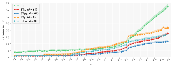
(a) sum

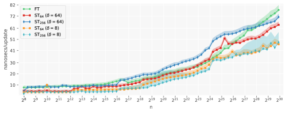
(b) update

Figure 21. The running times of sum/update for the $b$-ary Segment-Tree with branching factor 64 and 256.

We first consider the most general case where $\delta=64$. Regarding sum queries, we see that the two-level node layout, which guarantees constant-time complexity, together with the very short tree height, makes both the tested Segment-Tree versions substantially improve over the Fenwick-Tree. The curves for the Segment-Tree are strictly sandwiched between 1 and 2 nanoseconds until the data structures cannot be contained in $L_{2}$, which happens close to the $2^{17}$ boundary. In this region, the Segment-Tree is bound by the CPU cycles, whereas the Fenwick-Tree by branch misprediction. For $n\approx 2^{16}$ and sum queries, the ${\textup{{ST}}}_{64}$ executes 23% of the instructions and 22% of the cycles of the Fenwick-Tree. As a result of the optimizations we discussed at the beginning of the section (loop-unrolling and reduced branches), it only performs 2.2% of the branches of the Fenwick-Tree and misses 0.36% of those. The larger tree height of the Fenwick-Tree also induces a poor cache utilization compared to the Segment-Tree. As already discussed, this becomes evident for large values of $n$. For example, for $n=250\times 10^{6}$ and sum queries, ${\textup{{ST}}}_{64}$ incurs in 40% less cache misses than the Fenwick-Tree (and ${\textup{{ST}}}_{256}$ in 80% less). This cache-friendly behavior is a direct consequence of the very short height.

Perhaps more interesting is the case for updates, where SIMD instructions can be exploited to lower the running time. As a reference point, we show in Figure 22 the running time of update without manual usage of SIMD (only the general case is shown for simplicity): compared to the plots in Figure 21, we see that SIMD offers a good reduction in the running time of update. If we were not to use SIMD, we would have obtained a $4\times$ lager time for update, thus SIMD is close to its ideal speed-up for our case (4 $\times$ 64-bit integers are packed in a register). This reduction is more evident for $b=64$ rather than $b=256$ because, as we discussed in Section 7.1, updating 8 keys is faster than updating 16 keys: this let the $\textup{{ST}}_{64}$ perform (roughly) half of the SIMD instructions of $\textup{{ST}}_{256}$, although $\textup{{ST}}_{256}$ is one level shorter. This translates into fewer spent cycles and less time. Also, ${\textup{{ST}}}_{256}$ incurs in a bit more cache misses than ${\textup{{ST}}}_{64}$, 11% more, because each update must access the double of cache lines than ${\textup{{ST}}}_{64}$: from Section 7.1, recall that each segment consists of 16 keys that fit in two cache lines. Instead, the $\textup{{ST}}_{64}$ solution is as fast or better than the Fenwick-Tree thanks to SIMD instructions. Is is important to stress that $\textup{{ST}}_{64}$ actually executes more instructions then the Fenwick-Tree. However, it does so in fewer cycles, thus confirming the good impact of SIMD.

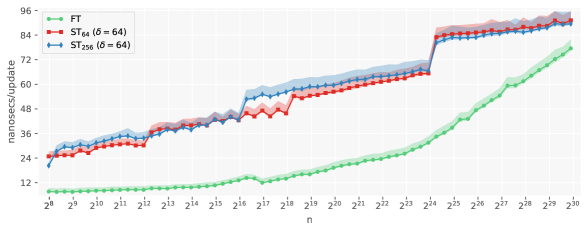
Figure 22. The running times of update for the $b$-ary Segment-Tree with branching factor 64 and 256, without manual usage of SIMD instructions.

Considering the overall trade-off between sum and update, we conclude that – for the general case where $\Delta$ is expressed in 8 bytes – the ${\textup{{ST}}}_{64}$ data structure offers the best running times.

We now discuss the case where $\delta=8$. Queries are less efficient than those in the general case because, as explained in Section 7.1, they are computed by accessing four different array locations at each level of the tree. These additional accesses to memory induce more cache-misses as soon as the data structure does not fit in cache: in fact, notice how the time rises around $2^{12}$ and $2^{16}$ boundaries, also because the restricted versions consume more space. Anyway, the $\textup{{ST}}_{256}$ variant maintains a good advantage against the Fenwick-Tree, especially on the large values of $n$ (its curve is actually very similar to that of ${\textup{{ST}}}_{64}$ for the general case).

The restriction on $\Delta$ produces an improvement for update as expected. Note how the shape of $\textup{{ST}}_{256}$ dramatically improves (by $1.5-2\times$) in this case because 16 keys are updated in parallel rather than just 4 as in the general case (now, 16 $\times$ 16-bit integers are packed in a register).

Therefore, we conclude that – for the restricted case where $\Delta$ is expressed in 1 byte – the solution $\textup{{ST}}_{256}$ offers the best trade-off between the running times of sum and update.

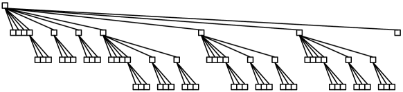
(a) $b$-ary Fenwick-Tree

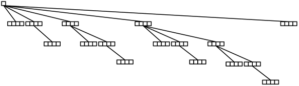
(b) blocked Fenwick-Tree

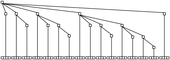
(c) truncated Fenwick-Tree

Figure 23. The shapes of different data structures with $b=4$, built from an input array of size 64, and based on the Fenwick-Tree.

8. The $b$-ary Fenwick-Tree

The classic Fenwick-Tree we described in Section 5 exploits the base-2 representation of a number in $[0,n)$ to support sum and update in time $O(\log n)$. If we change the base of the representation to a value $b>2$, the corresponding $b$-ary Fenwick-Tree can be defined (Bille et al., 2017) – a data structure supporting sum in $O(\log_{b}n)$ and update in $O(b\log_{b}n)$. A pictorial representation of the data structure is given in Figure 23a for $b=4$ and $n=64$. However, this data structure does not expose an improved trade-off compared to the solutions described in the previous sections, for the reasons we discuss in the following.

Let us consider sum. Recall that the Fenwick-Tree ignores digits that are 0. We have already commented on this for the case $b=2$ in Section 6: for random queries, this gives a consistent boost over the Segment-Tree with $b=2$ because roughly 50% of the levels are skipped, as if the height of the tree were actually $\frac{1}{2}\lceil\log_{2}(n+1)\rceil$. Unfortunately, this advantage does not carry over for larger $b$ because the probability that a digit is 0 is $1/b$ which is very low for the values of $b$ we consider in our experimental analysis (64 and 256). In fact, the $b$-ary Fenwick-Tree is not faster than the $b$-ary Segment-Tree (although it is when compared to the classic Fenwick-Tree with $b=2$).

Even more problematic is the case for update. Having to deal with more digits clearly slows down update that needs to access $b-1$ nodes per level, for a complexity of $O(b\log_{b}n)$. Observe that $(b-1)\frac{\log_{2}n}{\log_{2}b}$ is more than $\log_{2}n$ for every $b>2$. For example, for $b=64$ we can expect a slowdown of more than $10\times$ (and nearly $32\times$ for $b=256$). Experimental results confirmed this analysis. Note that the $b$-ary Segment-Tree does much better than this because: (1) it traverses $\lceil\log_{b}n\rceil$ nodes for operation, (2) the $b$ keys to update per node are contiguous in memory for a better cache usage and, hence, (3) are amenable to the SIMD optimizations we described in Section 7.1. Therefore, we experimented with two other ideas in order to improve the trade-off of the $b$-ary Fenwick-Tree.

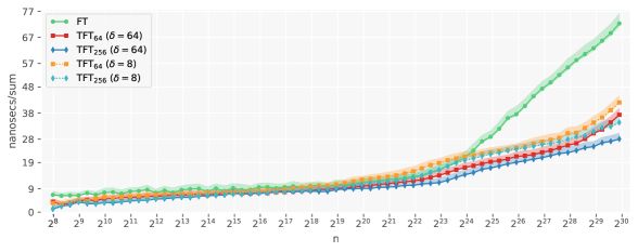
(a) sum

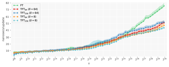
(b) update

Figure 24. The running times of sum/update for the truncated Fenwick-Tree (TFT) with leaves of 64 and 256 keys.

The first idea is to block $b$ keys together into the nodes of a classic Fenwick-Tree, as depicted in Figure 23b for $b=4$ and $n=64$. Compared to the $b$-ary Fenwick-Tree, this variant – that we call the blocked Fenwick-Tree – slows down the queries but improves the updates, for a better trade-off. However, it does not improve over the classic Fenwick-Tree with $b=2$. In fact, although the height of the tree is $\lceil\log_{2}((n+1)/b)\rceil+1$, thus smaller than that of the classic Fenwick-Tree by $\log_{2}b$, the number of traversed nodes is only reduced by $\frac{1}{2}\log_{2}b$, which is quite small for the values of $b$ considered (e.g., just 3 for $b=64$). Therefore, this variant traverses slightly fewer nodes but the computation at each node is more expensive (more cache lines accessed due to two-level nodes; more cycles spent due to SIMD), resulting in a larger runtime compared to the classic Fenwick-Tree.

This suggests the implementation of a strategy where one keeps running the simplest code for update, e.g., that of the classic Fenwick-Tree, until the number of leaves in the sub-tree is $b$ and, thus, these can be updated in parallel with SIMD. The shape of the resulting data structure – the truncated Fenwick-Tree (TFT) – is illustrated in Figure 23c (for $b=4$ and $n=64$) and shows the clear division between the upper part represented by the Fenwick-Tree and the lower part that consists in an array of blocks. Compared to the classic Fenwick-Tree, it is now intuitive that this variant reduces the number of cache-misses because the upper part is likely to fit well in cache and $b$ keys inside a block are contiguous in memory.

The experimental results shown in Figure 24 meet our expectations, as the truncated variant actually improves over the classic Fenwick-Tree. In particular, it performs similarly to the Fenwick-Tree for small values of $n$ but gains a significant advantage for larger $n$ thanks to its better cache usage. Comparing Figure 24b to Figure 21b at page 21b, we can also observe that this variant improves over the $b$-ary Segment-Tree in the general case for update ($\delta=64$) and large $n$ because the use of SIMD is limited to one block of $b$ keys per operation. For sum queries instead, the data structure performs similarly to the $b$-ary Segment-Tree, with the latter being generally faster for all values of $n$.

As last note, we remark that all the variants of the Fenwick-Tree we sketched in this section are anyway part of the software library available at https://github.com/jermp/psds.

9. Conclusions and future work

We described, implemented, and studied the practical performance of several tree-shaped data structures to solve the prefix-sum problem. After a careful experimental analysis, the following take-away lessons are formulated.

1. (Section 4) A bottom-up traversal of the Segment-Tree has a much simpler implementation compared to top-down, resulting in a faster execution of both sum and update.

2. (Section 4) A branch-free implementation of the Segment-Tree is on average $2\times$ faster than a branchy implementation for all array sizes, $n$, up to $2^{25}$. This is so because the processor’s pipeline is not stalled due to branches, for a consequent increase in the instruction throughput. For $n>2^{25}$, the branchy code is faster because it saves memory accesses – the dominant cost in the runtime for large values of $n$.

   In particular, the combination of branchy and branch-free code execution – what we called the two-loop optimization – results in a better runtime.

   Taking this into account, we recommend a version of the bottom-up Segment-Tree where an internal node holds the sum of the leaves descending from its left subtree, because it allows the use of the two-loop optimization for update as well (and not only for sum).

3. (Section 5) The Fenwick-Tree suffers from cache conflicts for larger values of $n$, caused by accessing nodes whose memory address is (almost) a large power of 2. Solving this issue, by offsetting a node from an original position $i$ to a new position $i+\lfloor i/d\rfloor$ for some $d>0$, significantly improves the performance of the Fenwick-Tree.

   Table 2. Average speedup factors achieved by the Fenwick-Tree over the Segment-Tree.

   Array Size	sum		update
   $2^{8}<n\leq 2^{16}$	1.32$\times$		1.17$\times$
   $2^{16}<n\leq 2^{22}$	2.43$\times$		1.64$\times$
   $2^{22}<n\leq 2^{30}$	1.82$\times$		1.50$\times$

4. (Section 6) The Fenwick-Tree is more efficient than (our optimized version of) the Segment-Tree for both queries and updates. The better efficiency is due to the simplicity of the code and the less (50%) average number of loop iterations. We summarize the speedups achieved by the Fenwick-Tree over the Segment-Tree in Table 2, for different ranges of $n$.

5. (Section 7) Although the Segment-Tree is outperformed by the Fenwick-Tree, we can enlarge its branching factor to a generic quantity $b>2$: this reduces the height of the Segment-Tree for a better cache usage and enables the use of SIMD instructions. Such instructions are very effective to lower the running time of update, because several values per node can be updated in parallel.

   Compared to the scalar update algorithm, SIMD can be on average $2-6\times$ faster depending of the value of $n$.

6. (Section 7) For the best of performance, we recommend to model the height of the $b$-ary Segment-Tree with a constant known at compile-time, so that the compiler can execute a specialized code path to handle the specific value of the height. This completely avoids branches during the execution of sum and update.

   The vectorized update implementation together with this branch-avoiding optimization makes the $b$-ary Segment-Tree actually faster than the Fenwick-Tree. We report the speedups achieved by this data structure over the Fenwick-Tree in Table 3, for the different tested combinations of $b$ and $\delta$. (Recall that $\delta$ represents the bit-width of $\Delta$, the update value.)

7. (Section 7) For the most general case where $\delta=64$ bits, we recommend the use of a $b$-ary Segment-Tree with $b=64$. From Table 3, we see that this solution offers an improved trade-off between the running time of sum and update: on average $1.9-5\times$ faster for sum and up to $1.6\times$ faster for update than the Fenwick-Tree.

8. (Section 7) For the restricted case where $\delta=8$ bits, we can update even more values in parallel by buffering the updates at each node of the tree. Considering again Table 3, for such case we recommend the use of a $b$-ary Segment-Tree with $b=256$. This solution is faster than a Fenwick-Tree by $1.7-4.7\times$ for sum and by $1.4-2.5\times$ for update.

9. (Section 8) The $b$-ary Fenwick-Tree improves the runtime for queries at the price of a significant slowdown for updates, compared to the classic Fenwick-Tree with $b=2$. This makes the data structure unpractical unless updates are extremely few compared to queries.

10. (Section 8) Despite of the larger tree height, the blocked Fenwick-Tree improves the trade-off of the $b$-ary Fenwick-Tree (in particular, it improves update but worsens sum). However, it does not beat the classic Fenwick-Tree because the time spent at each traversed node is much higher (more cache-misses due to the two-level structure of a node; more spent cycles due to SIMD).

11. (Section 8) In order to combine the simplicity of the Fenwick-Tree with the advantages of blocking $b$ keys together (reduced cache-misses; SIMD exploitation), a truncated Fenwick-Tree can be used. This data structure improves over the classic Fenwick-Tree, especially for large values of $n$, exposing a trade-off similar to that of the $b$-ary Segment-Tree (but with the latter being generally better).

Table 3. Average speedup factors achieved by the $b$-ary Segment-Tree over the Fenwick-Tree.

$\delta$	64			8
$b$	64	256		64	256
$\,\,2^{8}<n\leq 2^{16}$	5.29$\times$	6.57$\times$		3.28$\times$	4.66$\times$
$2^{16}<n\leq 2^{22}$	2.58$\times$	3.24$\times$		1.11$\times$	1.54$\times$
$2^{22}<n\leq 2^{30}$	1.90$\times$	2.56$\times$		1.27$\times$	1.66$\times$

(a) sum

$\delta$	64			8
$b$	64	256		64	256
$\,\,2^{8}<n\leq 2^{16}$	1.62$\times$	1.08$\times$		2.08$\times$	2.52$\times$
$2^{16}<n\leq 2^{22}$	1.16$\times$	0.82$\times$		1.56$\times$	1.72$\times$
$2^{22}<n\leq 2^{30}$	1.05$\times$	0.88$\times$		1.35$\times$	1.40$\times$

(b) update

Some final remarks follow. The runtime of update will improve as SIMD instructions will become more powerful in future years (e.g., with lower latency), thus SIMD is a very promising hardware feature that cannot be overlooked in the design of practical algorithms.

So far we obtained best results using SIMD registers of 128 and 256 bits (SSE and AVX instruction sets, respectively). We also made some experiments with the new AVX-512 instruction set which allows us to use massive load and store instructions comprising 512 bits of memory. In particular, doubling the size of the used SIMD registers can be exploited in two different ways: by either reducing the number of instructions, or enlarging the branching factor of a node. We tried both possibilities but did not observe a clear improvement.

A promising avenue for future work would be to consider the searchable version of the problem, i.e., to implement the search operation. Note that this operation is actually amenable to SIMD vectorization, and has parallels with search algorithms in inverted indexes. With this third operation, the objective would be to use (a specialization of) the best data structure from this article – the $b$-ary Segment-Tree with SIMD on updates and searches – to support rank/select queries over mutable bitmaps (Marchini and Vigna, 2020), an important building block for dynamic succinct data structures.

The experiments presented in this work were conducted using a single system configuration, i.e., a specific processor (Intel i9-9940X), operating system (Linux), and compiler (gcc). We acknowledge the specificity of our analysis, although it involves a rather common setup, and we plan to extend our experimentation to other configurations as well in future work.

10. ACKNOWLEDGMENTS

This work was partially supported by the BigDataGrapes (EU H2020 RIA, grant agreement N^o̱780751), the “Algorithms, Data Structures and Combinatorics for Machine Learning” (MIUR-PRIN 2017), and the OK-INSAID (MIUR-PON 2018, grant agreement N^o̱ARS01_00917) projects.

References

- (1)
- Bentley (1977) Jon Louis Bentley. 1977. Solutions to Klee’s rectangle problems. Unpublished manuscript (1977), 282–300.
- Bentley and Wood (1980) Jon Louis Bentley and Derick Wood. 1980. An optimal worst case algorithm for reporting intersections of rectangles. IEEE Trans. Comput. 7 (1980), 571–577.
- Bille et al. (2018) Philip Bille, Anders Roy Christiansen, Patrick Hagge Cording, Inge Li Gørtz, Frederik Rye Skjoldjensen, Hjalte Wedel Vildhøj, and Søren Vind. 2018. Dynamic relative compression, dynamic partial sums, and substring concatenation. Algorithmica 80, 11 (2018), 3207–3224.
- Bille et al. (2017) Philip Bille, Anders Roy Christiansen, Nicola Prezza, and Frederik Rye Skjoldjensen. 2017. Succinct partial sums and fenwick trees. In International Symposium on String Processing and Information Retrieval. Springer, 91–96.
- Blelloch (1990) Guy E. Blelloch. 1990. Prefix Sums and Their Applications. Synthesis of Parallel Algorithms (1990).
- Brodnik et al. (2006) Andrej Brodnik, Johan Karlsson, J Ian Munro, and Andreas Nilsson. 2006. An O (1) solution to the prefix sum problem on a specialized memory architecture. In Fourth IFIP International Conference on Theoretical Computer Science-TCS 2006. Springer, 103–114.
- Chan and Pătraşcu (2010) Timothy M. Chan and Mihai Pătraşcu. 2010. Counting inversions, offline orthogonal range counting, and related problems. In Proceedings of the twenty-first annual ACM-SIAM symposium on Discrete Algorithms. SIAM, 161–173.
- Corporation (2020) Intel Corporation. [last accessed June 2020]. The Intel Intrinsics Guide, https://software.intel.com/sites/landingpage/IntrinsicsGuide/.
- de Berg et al. (2008) Mark de Berg, Otfried Cheong, Marc J. van Kreveld, and Mark H. Overmars. 2008. Computational geometry: algorithms and applications, 3rd Edition. Springer.
- Dietz (1989) Paul F. Dietz. 1989. Optimal algorithms for list indexing and subset rank. In Workshop on Algorithms and Data Structures. Springer, 39–46.
- Fenwick (1994) Peter M. Fenwick. 1994. A new data structure for cumulative frequency tables. Software: Practice and experience 24, 3 (1994), 327–336.
- Fredman and Saks (1989) Michael L. Fredman and Michael E. Saks. 1989. The Cell Probe Complexity of Dynamic Data Structures. In Proceedings of the 21-st Annual Symposium on Theory of Computing (STOC). 345–354.
- Goodman et al. (2017) Jacob E. Goodman, Joseph O’Rourke, and Csaba D. Toth. 2017. Handbook of discrete and computational geometry. CRC press. https://www.csun.edu/~ctoth/Handbook/HDCG3.html
- Goodrich et al. (1994) Michael T Goodrich, Yossi Matias, and Uzi Vishkin. 1994. Optimal parallel approximation for prefix sums and integer sorting. In SODA. 241–250.
- Gray et al. (1997) Jim Gray, Surajit Chaudhuri, Adam Bosworth, Andrew Layman, Don Reichart, Murali Venkatrao, Frank Pellow, and Hamid Pirahesh. 1997. Data cube: A relational aggregation operator generalizing group-by, cross-tab, and sub-totals. Data mining and knowledge discovery 1, 1 (1997), 29–53.
- Hampapuram and Fredman (1998) Haripriyan Hampapuram and Michael L. Fredman. 1998. Optimal biweighted binary trees and the complexity of maintaining partial sums. SIAM J. Comput. 28, 1 (1998), 1–9.
- Harris et al. (2007) Mark Harris, Shubhabrata Sengupta, and John D Owens. 2007. Parallel prefix sum (scan) with CUDA. GPU gems 3, 39 (2007), 851–876.
- Hon et al. (2011) Wing-Kai Hon, Kunihiko Sadakane, and Wing-Kin Sung. 2011. Succinct data structures for searchable partial sums with optimal worst-case performance. Theoretical computer science 412, 39 (2011), 5176–5186.
- Khuong and Morin (2017) Paul-Virak Khuong and Pat Morin. 2017. Array layouts for comparison-based searching. Journal of Experimental Algorithmics (JEA) 22 (2017), 1–39.
- Marchini and Vigna (2020) Stefano Marchini and Sebastiano Vigna. 2020. Compact Fenwick trees for dynamic ranking and selection. Software: Practice and Experience 50, 7 (2020), 1184–1202.
- Meijer and Akl (1987) Henk Meijer and Selim G Akl. 1987. Optimal computation of prefix sums on a binary tree of processors. International Journal of Parallel Programming 16, 2 (1987), 127–136.