Auditory streaming emerges from fast excitation and slow delayed inhibition

Abstract

In the auditory streaming paradigm alternating sequences of pure tones can be perceived as a single galloping rhythm (integration) or as two sequences with separated low and high tones (segregation). Although studied for decades, the neural mechanisms underlining this perceptual grouping of sound remains a mystery. With the aim of identifying a plausible minimal neural circuit that captures this phenomenon, we propose a firing rate model with two periodically forced neural populations coupled by fast direct excitation and slow delayed inhibition. By analyzing the model in a non-smooth, slow-fast regime we analytically prove the existence of a rich repertoire of dynamical states and of their parameter dependent transitions. We impose plausible parameter restrictions and link all states with perceptual interpretations. Regions of stimulus parameters occupied by states linked with each percept matches those found in behavioral experiments. Our model suggests that slow inhibition masks the perception of subsequent tones during segregation (forward masking), while fast excitation enables integration for large pitch differences between the two tones.

fnextchar@ifnextchar

Research

1 Introduction

Understanding how our perceptual system encodes multiple objects simultaneously is an open challenge in sensory neuroscience. In a busy room we can separate out a voice of interest from other voices and ambient sound (cocktail party problem) [1, 2]. Theories of feature discrimination developed with mathematical models are based on evidence that different neurons respond to different stimulus features (e.g. visual orientation [3, 4, 5, 6]). Primary auditory cortex (ACx) has a topographic map of sound frequency (tonotopy): a gradient of locations preferentially responding to frequencies from low to high [7, 8]. However, feature separation alone cannot account for the auditory system segregating objects overlapping or interleaved in time (e.g. melodies, voices). Understanding the role of temporal neural mechanisms in perceptual segregation presents an interesting modelling challenge where the same neural populations represent different percepts through temporal encoding.

1.1 Auditory streaming and auditory cortex

In the auditory system sequences of sounds (streams) that are close in feature space (e.g. frequency) and interleaved in time lead to multiple perceptual interpretations. The so-called auditory streaming paradigm [9, 2] consists of interleaved sequences of tones A and B, separated by a difference in tone frequency (called $df$) and repeating in an ABABAB…pattern (Figure 1A). This can be perceived as one integrated stream with an alternating rhythm (Integrated in Figure 1B) or as two segregated streams (Segregated in Figure 2B). When $df$ is small we hear integrated and when df is large we hear segregated, but at an intermediate range, which also depends on presentation rate $P\!R$, both percepts are possible (Figure 1C). In this region of $(\text{df},{P\!R})$ parameter space bistability occurs, where perception switches between integrated and segregated every 2–15 s [10]. The curve separating integration and bistability is called the fission boundary, while the curve separating bistability and segregation is called coherence boundary [9] (Figure 1C).

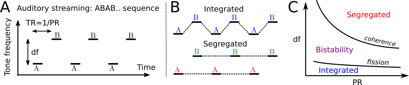
Figure 1: The auditory streaming paradigm (A) Auditory stimuli consist of sequences of interleaved higher pitch A and lower pitch B pure tones with duration $T\!D$, pitch difference $df$ and time difference between tone onsets $T\!R$ (the repetition time; $P\!R\!=\!1/T\!R$ is the repetition rate). (B) The stimulus may be perceived as either an integrated ABAB stream or as two separate streams A-A- and -B-B. (C) Sketch of the perceptual regions when varying $P\!R$ and $d\!f$ (van Noorden diagram), redrawn after [9]. Bistability corresponds to the perception of temporal switches between integration and segregation. The curves in the $(P\!R,df)$ space separating integration from bistability and bistability from segregation are called fission and coherence boundaries.

Figure 2A shows our proposal for the encoding of auditory streaming. We follow the hypothesis proposed by [11], where primary and secondary ACx encode respectively perception of the rhythm and the pitch. In our proposed framework the processing of auditory stimuli occurs firstly in primary ACx, which projects to secondary ACx. The various rhythms occurring in the auditory streaming paradigm arise via threshold-crossing detection in the activity of neural populations in secondary ACx. The process underlying bistability is likely resolved downstream of early auditory cortex [12] and will not be addressed in this study.

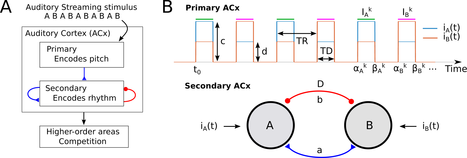
Figure 2: (A) Proposed modelling framework of the auditory streaming paradigm. Two-tone streams are processed in primary ACx. Seconday ACs receives inputs from primary areas and has recurrent excitatory and inhibitory connections. Primary and secondary areas encode respectively pitch and rhythm [11], while high-order cortical areas encode the perceptual switches via competition (bistability). (B) ACx circuit model. Primary ACx tonotopic responses consist of square-wave A and B tone inputs $i_{A}$ and $i_{B}$ with duration $T\!D$ and with the time between tone onsets $T\!R$ (called repetition time - the inverse of the presentation rate (PR)). Parameters $c$ and $d$ respectively represent the connection strength from $i_{A}$ ($i_{B}$) to the A(B) and B(A) units. Bottom: sketch of the model circuit consisting of two mutually excitatory and inhibitory populations with strengths $a$ and $b$ respectively, receiving inputs $i_{A}$ and $i_{B}$. Inhibition is delayed of the amount $D$.

1.2 Existing models of auditory streaming

Inspired by evidence of feature separation shown in neural recordings in primary auditory cortex (A1) [13], many existing models have sidestepped the issue of the temporal encoding of the perceptual interpetations by focusing on a feature representation (reviews: [14, 15, 12]). Neurons responding primarily to the A or to the B tones are in adjacent locations, spatially separated along A1’s tonotopic axis. The so-called neuromechanistic model [16] proposed the encoding of percepts based on discrete, tonotopically organised units interacting through plausible neural mechanisms. Models proposed in a neural oscillator framework feature significant redunancy in their structure or work only at specific presentation rate (PR) values [17, 18]. Temporal forward masking results in weaker responses to similar sounds that are close in time (at high PR), but this ubiquitous feature of the auditory system [19] has been overlooked in previous models.

1.3 Theoretical framework.

The cortical encoding of sensory information involves large neural populations suitably represented by coarse-grained variables like the mean firing rate. The Wilson-Cowan equations [20] considered here describe neural populations with excitatory and delayed inhibitory coupling. Variants of these equations include networks with excitatory and inhibitory coupling, intrinsic synaptic dynamics that include neural adaptation, nonlinear gain functions [21, 22, 23] and symmetries [24, 25]. This framework (and related voltage- or conductance-based formulations) are widely used to study e.g. decision making [26], perceptual competition in the visual [27, 24, 28] and in the auditory system [16]. Mathematical studies of these models often use a discontinuous (Heaviside) gain function due to its analytical tractability [29].

A range of neural and synaptic activation times often leads to timescale separation [30, 31, 32] as considered here. Singular perturbation theory has been instrumental in revealing the dynamic mechanisms behind neural behaviors involving a slow-fast decomposition, e.g. the generation of spiking and bursting [31, 33], neural competition [23, 34] and rhythmic behaviors [35, 36]. In this work we use these techniques to determine the existence conditions of various dynamical states.

We consider the role of delayed inhibition in generating oscillatory activity compatible with auditory percepts. Delayed inhibition produces similar patterns of in- and anti-phase oscillations in spiking neural models [37, 38]. Delays in small neural circuits [39] lead to many interesting phenomena including inhibition-induced Hopf oscillations, oscillator death, multistability and switching between oscillatory solutions [40, 41]. Two novel features of our study are that the units are not intrinsically oscillating and that periodic forcing drives oscillations. Periodically forced, timescale separated models of perceptual competition [42, 28, 18] typically do not feature delays.

1.4 Outline

With the aim of clarifying a plausible model for the processing of ambiguous sounds we present a biologically-inspired neural circuit in ACx with mixed feature and temporal encoding (Section 2). Section 3 describes numerical simulations of the model states linked to percepts in the auditory streaming paradigm. Later sections focus on the analytical derivation of existence conditions for these states in a non-smooth, slow-fast regime. Proofs of most of these results are given in the Supplementary Material for the interested reader. In Sections 4 we dissect the model into slow and fast subsystems then analyze quasi-equilibria of the fast subsystem. We use this analysis in Sections 5 and 6 to classify dynamical states with binary matrix representations (matrix form). This tool determines all periodic states, their existence conditions and which states are impossible. Sections 7 and 8 classify periodic states for long and short inhibitory delays, respectively. Lastly, in Section 9 we show with numerics how these results extend to a smooth setting with reduced timescale separation. Overall, we propose a new method for analytically determining the solutions of a periodically driven networks in a slow-fast setting with delays. When applied to study the auditory streaming paradigm, these methods suggest how competing perceptual interpretations emerge as a result of mutual excitation and slow delayed inhibition in tonotopically localized units in a non-primary part of auditory cortex.

2 The mathematical model

We present a model for the encoding of different perceptual interpretations of the auditory streaming paradigm. Following our proposal of rhythm and pitch perception (Figure 2A) we consider a periodically-driven competition network of two localised Wilson-Cowan units (Figure 2B) with lumped excitation and inhibition generalised to include dynamics via inhibitory synaptic variables. The units A and B are driven by a stereotyped input signals $i_{A}$ and $i_{B}$ representative of neural responses in primary auditory cortex [13] at tonotopic locations that preferentially respond to A and to B tones (Figure 2B). The model is described by the following system of DDEs:

$$\begin{array}[]{lcl}\tau\dot{u}_{A}(t)&=&-u_{A}(t)+H(au_{B}(t)-bs_{B}(t-D)+ci_{A}(t)),\\ \tau\dot{u}_{B}(t)&=&-u_{B}(t)+H(au_{A}(t)-bs_{A}(t-D)+ci_{B}(t)),\\ \dot{s}_{A}(t)&=&H(u_{A}(t))(1-s_{A}(t))/\tau-s_{A}(t)/\tau_{i},\\ \dot{s}_{B}(t)&=&H(u_{B}(t))(1-s_{B}(t))/\tau-s_{B}(t)/\tau_{i},\end{array}$$ (1)

where units $u_{A}$ and $u_{B}$ represent the average firing rate of two neural populations encoding sequences of tone (sound) inputs with timescale $\tau$. The Heaviside gain function with activity-threshold $\theta\in(0,1)$: $\{H(x)\!=\!1$ if $x\geq\theta$ and 0 otherwise$\}$ is widely used in firing rate and neuronal field models [23, 43] (we later relax this assumption to consider a smooth gain function). Mutual coupling through direct fast excitation has strength $a\geq 0$. The delayed, slowly-decaying inhibition has timescale $\tau_{i}$, strength $b\geq 0$ and delay $D$ (Figure 2A). The synaptic variables $s_{A}$ and $s_{B}$ describe the time-evolution of the inhibitory dynamics. Typically we will assume $\tau_{i}$ to be large and $\tau$ to be small. This slow-fast regime and the choice of a Heaviside gain function allows for the derivation of analytical conditions for the existence of biologically relevant network states.

2.1 Model Inputs

We model primary ACx inputs to secondary areas as time-dependent, periodic square wave functions $i_{A}(t)$ and $i_{B}(t)$ representing the averaged excitatory synaptic currents from primary ACx at A and B tonotopic locations during the repetition of interleaved A and B tone sequences (Fig 2B top). These functions characterize responses to tones in primary ACx (from experiments [13]) rather than the sound waveform of the tone sequences (motivated in Section 3) and are defined by:

$$\begin{array}[]{lcl}i_{A}(t)&=c\sum_{k=0}^{\infty}\chi_{I_{A}^{k}}(t)+d\sum_{k=0}^{\infty}\chi_{I_{B}^{k}}(t)&\\ i_{B}(t)&=d\sum_{k=0}^{\infty}\chi_{I_{A}^{k}}(t)+c\sum_{k=0}^{\infty}\chi_{I_{B}^{k}}(t)&\end{array}$$ (2)

Where $c\!\geq\!0$ and $d\!\geq\!0$ represent the input strengths from A (B) tonotopic location respectively to the A (B) unit and to the B (A) unit; $\chi_{I}$ is the standard indicator function over the set $I$, defined as $\chi_{I}(t)\!=\!1$ for $t\in I$ and 0 otherwise. The intervals when A and B tones are on (active tone intervals) are respectively $I_{A}^{k}\!=\![\alpha_{k}^{A},\beta_{k}^{A}]$ and $I_{B}^{k}\!=\![\alpha_{k}^{B},\beta_{k}^{B}]$ (see Figure Fig 2B top), where α_A^k​=​2kT​R,  β_A^k​=​2kT​R​+​T​D,  α_B^k​=​(2k​+​1)T​R,  β_B^k​=​ (2k​+​1)T​R​+​T​D. Where the parameters $T\!D$ represents the duration of each tone’s presentation (see the Discussion for another interpretation of $T\!D$) and $T\!R$ the time between tone onsets (called repetition time; $P\!R\!=\!1/T\!R$ is the presentation rate). Let us name the set of active tone intervals $R$ and its union $I$ as Φ={ R ⊂R : R=I_k^A   or   R=I_k^B,   ∀k ∈N }  and  I=⋃_R ∈ΦR.

As shown in Figure 1, parameters $T\!D$ and $P\!R\!$ play an important influence on auditory streaming [13]. We consider $P\!R\in[1,40]$Hz, $T\!R\!\geq\!T\!D$ and $T\!R\!\geq\!D$, where $D$ is the inhibitory delay. These restrictions are typical conditions tested in psychoacoustic experiments. In particular, $T\!R\!\geq\!T\!D$ guarantees no overlaps between tone inputs, i.e. $I_{A}^{i}\cap I_{B}^{j}=\emptyset$, $\forall i,j\in\mathbb{N}$.

Remark 2.1 (Constraining model parameters).

Assuming $\tau$ sufficiently small and a Heaviside gain function $H$, system 1 with no inputs ($i_{A}\!=\!i_{B}\!=\!0$) has two possible equilibrium points: a quiescent state $P\!=\!(0,0,0,0)$ and an active state $Q\!=\!(1,1,1,1)$. If the difference between excitatory and inhibitory strengths $a\!-\!b\!\geq\!\theta$, then both $P$ and $Q$ exist, and any trajectory of the non-autonomous system is trivially determined by input strength $c$:

• If $c\!<\!\theta$: any trajectory starting from the basin of attraction of $P$ (or $Q$) quickly converges to $P$ ($Q$) and remains at this equilibrium.

• If $c\!\geq\!\theta$: any trajectory converges to $Q$ and remains at this equilibrium. Indeed, if an orbit is in the basin of $P$, the synaptic variables monotonically decrease until one unit turns ON. This turns ON the other unit (since $a\!-\!b\!\geq\!\theta$) and both units remain ON.

To avoid these unrealistic scenarios we assume the following conditions:

1. $a-b<\theta$

2. $c\geq\theta$

Condition ($U_{1}$) guarantees that the point $P=(0,0,0,0)$, representing a quiescent state, is the only equilibrium of system 1 with no inputs ($i_{A}=i_{B}=0$). Condition ($U_{2}$) guarantees inputs to be “strong enough” to turn ON the A (B) unit at the onset time of the A (B) tone in the absence of inhibition ($b=0$).

3 A motivating example

In this section we present examples of the type of responses studied throughout this work using a smooth version of model 1 and by proposing a link between these responses and the different percepts in the auditory streaming experiments. We use a sigmoid gain function $S(x)=[1+\exp(-\lambda x)]^{-1}$ with fixed slope $\lambda\!=\!30$. Inputs in 2 are made continuous using function $S$ by redefining them as:

$$\begin{split}I_{A}(t)=c\cdot p(t)p(T\!D\!-\!t)+d\cdot q(t)q(T\!D\!-\!t)\\ I_{B}(t)=d\cdot p(t)p(T\!D\!-\!t)+c\cdot q(t)q(T\!D\!-\!t)\end{split}$$ (3)

Where $p(t)\!=\!S(\sin(\pi P\!R\!\cdot\!t))$and $q(t)\!=\!S(-\sin(\pi P\!R\!\cdot\!t))$, so that the component $p(t)p(T\!D\!-\!t)$ ($q(t)q(T\!D\!-\!t)$) represents the responses to A (B) tone inputs with duration $T\!D$. These inputs are similar to the discontinuous input shown in Figure 2B but with smooth ramps at the discontinuous jump up and jump down points.

Psychoacoustic experiments systematically analysed the changes in perceptual outcomes when varying input parameters $P\!R$ and $df$ (Figure 1C). Parameter $P\!R$ is encoded in the model inputs’ repetition rates. To model parameter $df$ we take into account the experimental recordings of the average spiking activity from the primary ACx of various animals (macaque [13, 44], guinea pigs [45]). These recordings show that the average spiking activity at A tonotopic locations decreases non-linearly with $df$ during B tone presentations. We thus assume that the input strength $d$ can be scaled by $df$ according to $d\!=\!c\cdot(1\!-\!df^{1/m})$, where $m$ is a positive integer and $df$ is a unitless parameter in $[0,1]$ which may be converted to semitone units using the formula $12\log(1\!+\!df)$.

Figure 3A shows simulated time histories of all the $2T\!R$-periodic states for different values of parameters $(P\!R,df)$, where all the other parameters are fixed. Blue and red bars indicate the A and B active tone intervals $[0,T\!D]$ and $[T\!R,T\!R\!+\!T\!D]$, respectively, to show when the inputs are on. The system exhibits one of three possible behaviors: (1) a state in which both units cross threshold (total of 4 crossings), (2) a state in which the A unit crosses threshold twice and the B unit once (total of 3 crossings) and (3) a state in which both units cross threshold once (total of 2 crossings). We then summarize the effect of parameters $(P\!R,df)$ on the convergence to the different attractors by running massive simulations at varying parameters $(P\!R,df)$ and counting the number of threshold crossings (Figure 3B). States (1-3) belong to one of the grey regions in Figure 3B. We note that state (2) coexist with its complex conjugate state for which the B unit crosses threshold twice and the A unit once (not shown).

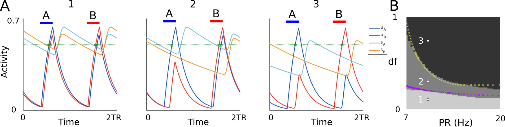
Figure 3: A. Time histories of the $2T\!R$-periodic states in system 1. Active tone A and B intervals are shown by blue and red bars, respectively. Units’ threshold crossings are shown by green dots. B. The total number of threshold crossings for both units is shown in greyscale for simulated trajectories at varying $P\!R$ and $df$ (black = $2$, lightest gray = $4$ crossings). Parameters $P\!R$ and $df$ in panel A are shown by white dots in panel B. Yellow and purple crosses are the experimentally detected coherence and fission boundaries respectively (data replotted from Figure 2 in [46], digitalized using the software WebPlotDigitizer [47]). The remaining parameters are $a\!=\!2$, $b\!=\!2.8$, $c\!=\!5.5$, $D\!=\!0.015$, $\theta\!=\!0.5$, $T\!D\!=\!0.022$, $\tau_{i}\!=\!0.25$, $\tau\!=\!0.025$, $\theta\!=\!0.5$ and $m\!=\!6$. Simulations are performed using dde23 in Matlab with absolute and relative tolerances set to $10^{-7}$. Initial conditions on the interval $[-D,0]$ are specified as a constant vector function equal to $[1,0,1,0]$.

We propose the following link between these states and the different percepts emerging in auditory streaming (integration, segregation and bistability). In our proposed framework rhythms are tracked by responding (threshold crossing) in the A and B units’ activities of $2T\!R$-periodic states. More precisely:

• Integration corresponds to state (1): both units respond to both tones.

• Bistability corresponds to state (2): one unit responds to both tones the other unit responds to only one tone.

• Segregation corresponds to state (3): no unit responds to both tones.

Following this proposal the states (1-3) match the regions of existence of their equivalent percepts. The transition boundaries between these states fit with the fission and coherence boundaries found experimentally (Figure 3B). In the next sections we take an analytical approach to study the model’s states and their existence conditions. This approach allows us to derive expressions for the fission and coherence boundaries (equations (25) in Section 8.1) in a mathematically tractable version of the model (2). Quantitative comparisons between the analytical and computational approaches are discussed in Section 9.

4 Fast dynamics

In this and the next sections (until Section 9) we present analytical results of the fast subsystem 4 with Heaviside gain. System 1 can decoupled into slow and fast subsystems. The fast subsystem is given by:

$$\begin{array}[]{lcl}u_{A}(r)^{\prime}&=&-u_{A}(r)+H(au_{B}(r)-bs_{B}(r-D)+i_{A}(r))\\ u_{B}(r)^{\prime}&=&-u_{B}(r)+H(au_{A}(r)-bs_{A}(r-D)+i_{B}(r))\\ s_{A}(r)^{\prime}&=&H(u_{A}(r))(1-s_{A}(r))\\ s_{B}(r)^{\prime}&=&H(u_{B}(r))(1-s_{B}(r))\end{array}$$ (4)

Where ${}^{\prime}=d/dr$ is the derivative with respect to the fast scale $r=t/\tau$. Activities $u_{A}$ and $u_{B}$ take a value of $0$ or $1$, or move rapidly (on the fast time scale) between these two values. We call A(B) ON if $u_{A}\sim 1$ and OFF if $u_{A}\sim 0$. The activity of the A (B) unit is determined by the sign of $au_{B}(t)\!-\!bs_{B}(t\!-\!D)\!+\!i_{A}(t)$ ($au_{A}(t)\!-\!bs_{A}(t-D)\!+\!i_{B}(t)$). Positive sign changes make $u_{A}$ ($u_{B}$) jump up from $0$ to $1$ (turn ON), while negative sign changes in make $u_{A}$ ($u_{B}$) jump down from $1$ to $0$ (turn OFF). The synaptic variables can act on either the fast or the slow time scales. If A (B) is ON the variable $s_{A}$ ($s_{B}$) jumps to 1 on the fast time scale. Instead, if A (B) is OFF the dynamics of $s=s_{A}$ (or $s=s_{B}$) slowly decay according to:

$$\dot{s}=-s/\tau_{i}$$ (5)

Remark 4.1.

The previous considerations demonstrate that $s_{A}(t)$ ($s_{B}(t)$) is a monotonically decreasing in time, except for when the A (B) unit makes an OFF to ON transition.

We proceed by analyzing the system at times $t\in I$, i.e. in one of the active tone intervals. WLOG from the definition of $I$ we assume that $t\in I_{k}^{A}$, a generic A tone interval. The analysis below can easily be extended for B tone intervals $I_{k}^{B}$ by swapping parameters $c$ and $d$. On the fast time scale the A and B unit satisfy the subsystem:

$$\begin{array}[]{lcl}u_{A}^{\prime}&=&-u_{A}+H(au_{B}-b\tilde{s}_{B}+c)\\ u_{B}^{\prime}&=&-u_{B}+H(au_{A}-b\tilde{s}_{A}+d)\end{array}$$ (6)

Where $\tilde{s}_{A}\!=\!s_{A}(t\!-\!D)$ and $\tilde{s}_{B}\!=\!s_{B}(t\!-\!D)$. System 6 has four equilibrium points: (0,0), (1,0), (0,1) and (1,1), and their existence conditions are reported in Table 1.

Equilibrium	(0,0)	(1,0)	(0,1)	(1,1)
Conditions	$\begin{aligned} c\!&<\!b\tilde{s}_{B}\!+\!\theta\\ d\!&<\!b\tilde{s}_{A}\!+\!\theta\\ \end{aligned}$	$\begin{aligned} c\!&\geq\!b\tilde{s}_{B}\!+\!\theta\\ a+d\!&<\!b\tilde{s}_{A}\!+\!\theta\\ \end{aligned}$	$\begin{aligned} a+c\!&<\!b\tilde{s}_{B}\!+\!\theta\\ d\!&\geq\!b\tilde{s}_{A}\!+\!\theta\\ \end{aligned}$	$\begin{aligned} a+c\!&\geq\!b\tilde{s}_{B}\!+\!\theta\\ a+d\!&\geq\!b\tilde{s}_{A}\!+\!\theta\\ \end{aligned}$

Table 1: Equilibria and existence conditions for the fast subsystem 6

The full system 1 may jump between these equilibria due to the slow decay of the synaptic variables or when $s_{A}(t\!-\!D)$ and $s_{B}(t\!-\!D)$ jumps up to 1.

4.1 Basins of attraction

From the inequalities given in Table 1 we note that points $(1,0)$ and $(0,1)$ cannot coexist with any other equilibrium and thus have trivial basins of attraction. However, $(0,0)$ and $(1,1)$ may coexist under the following conditions:

$$\begin{array}[]{lcccl}b\tilde{s}_{B}+\theta-a&\leq&c&<&b\tilde{s}_{B}+\theta\\ b\tilde{s}_{A}+\theta-a&\leq&d&<&b\tilde{s}_{A}+\theta\end{array}$$ (7)

Thus we must have $a>0$, i.e. when the excitation is not absent in the model. To study the basin of attraction for these two equilibria, we consider the vector field of system 6. For convenience we introduce the following quantities: $s_{1}\!=\!(b\tilde{s}_{A}\!-\!c\!+\!\theta)/a$ and $s_{2}\!=\!(b\tilde{s}_{B}\!-\!c\!+\!\theta)/a$. Conditions 7 hold if and only if $0<s_{k}\leq 1$, for $k=1,2$. Thus we can rewrite system 6 as:

$$\begin{array}[]{lcl}u_{A}^{\prime}&=&-u_{A}+H(a(u_{B}-s_{2}))\\ u_{B}^{\prime}&=&-u_{B}+H(a(u_{A}-s_{1}))\end{array}$$ (8)

Since $H$ is the Heaviside function $a$ can be removed. Figure 4 shows an example basins of attraction for parameter values for which $(0,0)$ and $(1,1)$ coexist (black circles). The $u_{A}$- and $u_{B}$-nullclines are shown in blue and red, respectively. We simulated model 8 starting from several initial conditions, covering the phase space. Simulated trajectories converge either to $(0,0)$ (green) and $(1,1)$ (purple) and show the subdivision in the basin of attraction.

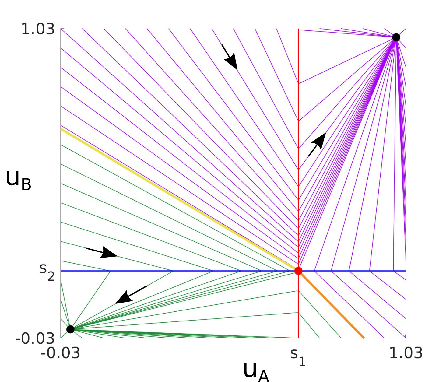
Figure 4: Phase portrait for system 8 with $s_{1}\!=\!0.7$ and $s_{2}\!=\!0.4$. Purple and green lines show orbits converging to $(1,1)$ and $(0,0)$, respectively (black circles). Black arrows indicate the direction of convergence. The $u_{A}$- and $u_{B}$-nullclines are shown in blue and red, respectively. Yellow and orange lines show the separatrices of the degenerate saddle $(s_{1},s_{2})$ (red circle).

There is a degenerate fixed point $(s_{1},s_{2})$ (red dot), where separatrices (yellow and orange lines) originate, dividing the phase plane into the regions of attraction shown in the figure. In the Supplementary Material 11.1 we prove that these curves are give by:

$$\begin{cases}(u_{A}-1)s_{2}/(s_{1}-1)&\mbox{if }u_{A}\leq s_{1}\\ u_{A}(s_{2}-1)/s_{1}+1&\mbox{otherwise}\end{cases}$$

The computational analysis of the basin of attractions (including equilibria and separatrices) with steep sigmoidal gains is presented in the Supplementary Material LABEL:basin_sigmoid and leads to qualitatively similar results.

4.2 Differential convergence to $(1,1)$

We now study the differential rate of convergence of the variables $u_{A}$ and $u_{B}$ for parameter values where $(1,1)$ is the only stable equilibrium, for an orbit starting from $(0,0)$. We will use the results below to classify of states of system 1. For simplicity we consider the case $t\in I_{A}^{k}$, as in system 6. Similar considerations hold in the case $t\in I_{B}^{k}$. Obviously, $(0,0)$ cannot be an equilibria, thus at least one of the two conditions in Table 1 must not be met. There are three cases to consider:

1. If $c\!\!-b\tilde{s}_{B}\!\geq\!\theta$ and $d\!-\!b\tilde{s}_{A}\!\geq\!\theta$ both units turn ON simultaneously following each following the same dynamics $u^{\prime}\!=\!1\!-\!u$. An orbit starting from $(0,0)$ must therefore reach $(1,1)$ under the same exponential rate of convergence.

2. If $c\!-\!b\tilde{s}_{B}\!\geq\!\theta$, $d\!-\!b\tilde{s}_{B}\!<\!\theta$ and $a\!+\!d\!-\!b\tilde{s}_{A}\!\geq\!\theta$ unit B turns ON after A by some small delay $\delta$ ($\sim\tau$). Indeed from $d\!-\!b\tilde{s}_{B}\!<\!\theta$ and $a\!+\!d\!-\!b\tilde{s}_{A}\!\geq\!\theta$ there $\exists u^{*}\in(0,1]$: $au_{*}\!+\!d\!-\!b\tilde{s}_{A}\!=\!\theta$. Since $c\!-\!b\tilde{s}_{B}\!\geq\!\theta$ the fast subsystem reduces to:

   $$\begin{array}[]{lcl}u_{A}^{\prime}&=&1-u_{A}\\ u_{B}^{\prime}&=&-u_{B}+H(au_{A}-b\tilde{s}_{A}+d)\stackrel{{\scriptstyle{\mbox{\footnotesize{def}}}}}{{=}}-u_{B}+\eta(u_{A})\end{array}$$

   Thus, the dynamics of $u_{A}$ is independent of $u_{B}$. Consider an orbit starting $(0,0)$ at $r=0$. From the first equation $u_{A}(r)$ tends to $1$ exponentially as $r\rightarrow\infty$, reaching a point $u^{*}$ at time $r^{*}\!=\!\log[(1\!-\!u^{*})^{-1}]$. For $r\!<\!r^{*}$ we have $u_{A}(r)\!<\!u^{*}$, which yields $\eta(u_{A}(r))\!=\!0$. Since the orbit starts from $u_{B}=0$, it must remain constant and equal to zero $\forall r\!<\!r^{*}$. For $r\!\geq\!r^{*}$, $\eta(u_{A}(r))\!=\!1$ and $u_{A}(r)\rightarrow 1$ following the same dynamics as $u_{A}$ at time $r=0$. On the time scale $t\!=\!\tau r$ of system 1, the A unit precedes the B unit in converging to $1$ precisely after an infinitesimal delay

   $$\delta=\tau\log[(1\!-\!u^{*})^{-1}].$$ (9)

3. The case $d\!-\!b\tilde{s}_{A}\!\geq\!\theta$, $c\!-\!b\tilde{s}_{A}\!<\!\theta$ and $a\!+\!c\!-\!b\tilde{s}_{B}\!\geq\!\theta$ is analogous to the previous after replacing $u_{A}$ with $u_{B}$. In this case A turns ON a delay $\delta$ after B.

4.3 Fast dynamics for $t\in\mathbb{R}\!-\!I$

The analysis for times when inputs are OFF ($t\in\mathbb{R}\!-\!I$) follows analogously by posing $c\!=\!d\!=\!0$ in system 6. Thus $(0,0)$ is an equilibrium for any values of parameters and delayed synaptic quantities $\tilde{s}_{A}$ and $\tilde{s}_{B}$. Instead $(1,1)$ is an equilibrium when a​-​b~s_A ​≥​ θ and  a​-​b~s_B ​≥​ θ.

5 Dynamics in the intervals with no inputs ($\mathbb{R}\!-\!I$)

The study of equilibria for the fast subsystem described so far constraints the dynamics of the full system in the intervals with no inputs, i.e. in $\mathbb{R}\!-\!I$. The first constraint is that the units can either be both ON, both OFF, or both turning OFF at any time in $\mathbb{R}\!-\!I$ (Theorem below).

Theorem 1 (Dunamics ifn $\mathbb{R}\!-\!I$).

For any $t\in\mathbb{R}\!-\!I$:

1. If A or B is OFF at time $t$, both units are OFF in $(t,t^{*}]$, where t^*=min_s ∈I {s ¿ t }

2. If A or B is ON at time $t$, both units are ON in $[t_{*},t)$, where t_*=max_s ∈I {s ¡ t }

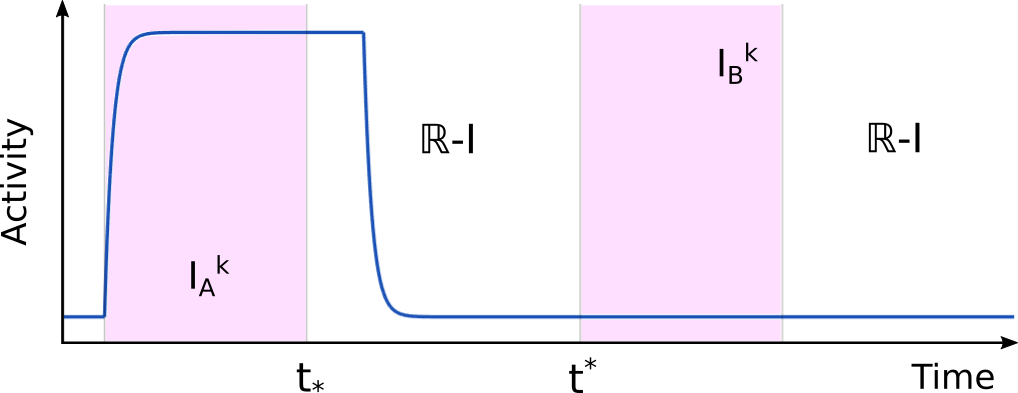
Figure 5: Illustration of Theorem 1 showing one unit’s dynamics (blue) during one $2T\!R$ period. Active tone intervals $I_{A}^{k}$ and $I_{B}^{k}$ are shown in purple. Note: the unit turns OFF at some time in $[t_{*},t^{*}]$ due to the delayed inhibition from the the other unit, whose activity is omitted.

This theorem is proved in the Supplementary Material LABEL:thm_ON_appendix and illustrated with an example in Figure 5. Due to this theorem we can classify network states as follows.

Definition 5.1 (LONG and SHORT states).

We define any state of system 1:

• LONG if $\exists t\in\mathbb{R}-I$ when both units are ON

• SHORT if both units are OFF $\forall t\in\mathbb{R}-I$

The choice of the names LONG and SHORT derives from the following considerations. Since both units are ON at some time $t\in\mathbb{R}-I$ of a LONG state, Theorem 1 implies they must be ON at time the end of the active tone interval preceding $t$ and prolong their activation after the active tone interval up to time $t$. SHORT states by definition are OFF between each pair of successive tone intervals.

Theorem 1 guarantees either unit can turn ON only during an active tone interval. This guarantees that the delayed synaptic variables are monotonically decreasing in the intervals $[\alpha_{k}^{A},\alpha_{k}^{A}\!+\!D]$ and $[\alpha_{k}^{B},\alpha_{k}^{B}\!+\!D]$ if the condition $T\!D\!+\!D\!<\!T\!R$ is guaranteed. The latter theorem is proven in the Supplementary Material LABEL:syn_decay_appendix and it is illustrated in Figure 6A.

Lemma 2 (synaptic decay).

If $T\!D\!+\!D<T\!R$ the delayed synaptic variables $s_{A}(t\!-\!D)$ and $s_{B}(t\!-\!D)$ are monotonically decreasing in $[\alpha_{k}^{A},\alpha_{k}^{A}\!+\!D]$ or $[\alpha_{k}^{B},\alpha_{k}^{B}\!+\!D]$, $\forall k\in\mathbb{N}$

A second important implication of Theorem 1 under $T\!D\!+\!D\!<\!T\!R$ is that both units must turn OFF once between successive tone intervals (see next lemma). This guarantees that at the start of each active tone interval any state of the fast subsystem start from point $(0,0)$. The following lemma is proven in the Supplementary Material LABEL:no_saturation_appendix and it is illustrated in Figure 6A.

Lemma 3 (no saturated states).

If $T\!D\!+\!D\!<\!T\!R$ both units are OFF in the intervals $(\alpha_{k}^{A}\!+\!T\!D+\!D,\alpha_{k}^{B}]$ and $(\alpha_{k}^{B}\!+\!T\!D+\!D,\alpha_{k+1}^{A}]$, $\forall k\in\mathbb{N}$.

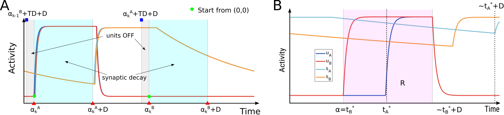
Figure 6: A. Example dynamics of the A and B units in each interval $L\subset\Gamma$ and $J$ illustrating lemmas 2 and 4 during one period $2T\!R$. B. Dynamics in an active tone interval $R\!=\![\alpha,\beta]\in\Phi$ illustrating the quantities in (1–3) of Lemma 4, where $t_{A}^{*}$ ($t_{B}^{*}$) is the turning ON time for A (B), respectively.

6 Dynamics during the active tone intervals

We now study the possible dynamics of the full system during the active tone intervals $R\in\Phi$ under the condition $T\!D\!+\!D\!<\!T\!R$, for which lemmas 2 and 3 can be applied. We split this analysis by separating the cases $D\!>\!TD$ and $D\!\leq\!TD$. In this section we consider the case $D\!>\!TD$, and the other conditions is considered in section 8. The next theorem shows that the turning ON times of either unit can happen only at most once in $R$ and other results which will lead to the existence of only a limited number of states.

Lemma 4 (single OFF to ON transition).

Consider an active tone interval $R\!=\![\alpha,\beta]\in\Phi$, and let A (B) be ON at a time $\bar{t}\in R$, then
(1) A (B) is ON $\forall t\geq\bar{t}$, $t\in R$
(2) $\exists!\,t_{A}^{*}\,(t_{B}^{*})\in R$ when A (B) turns ON
(3) $s_{A}(t\!-\!D)$ ($s_{B}(t\!-\!D)$) is decreasing for $t\in[\alpha,t_{A}^{*}\!+\!D]$ ($t\in[\alpha,t_{B}^{*}\!+\!D]$)

The previous Lemma is illustrated in the cartoon shown in Figure 6 right. The proof is given in the Supplementary Material LABEL:appendix_one_transition and it implies the following Lemma.

Lemma 5.

Given any active tone interval $R\in\Phi$ we have:

1. A (B) turns ON at time $\alpha$ $\Leftrightarrow$ A (B) is ON $\forall t\in(\alpha,\beta]$

2. A (B) is OFF at time $\beta$ $\Leftrightarrow$ A (B) is OFF $\forall t\in R$

Due to Lemma 4 each unit may turn ON only once during each interval $R\in\Phi$. Thus the dynamics any state is determined precisely at the jump up points $t_{A}^{*}$ and $t_{B}^{*}$ for the units in $R$ (if these exist).

Definition 6.1 (MAIN and CONNECT states).

Any state (solution) of system 1 is:

• MAIN if $\forall R\in\Phi$, if $\exists t^{*}\!\in\!R$ turning ON time for A or B, then $t^{*}\!=\!\min(R)$

• CONNECT if $\exists R\in\Phi$ and $\exists t^{*}\!\in\!R$, $t^{*}\!>\!\min(R)$ turning ON time for A or B

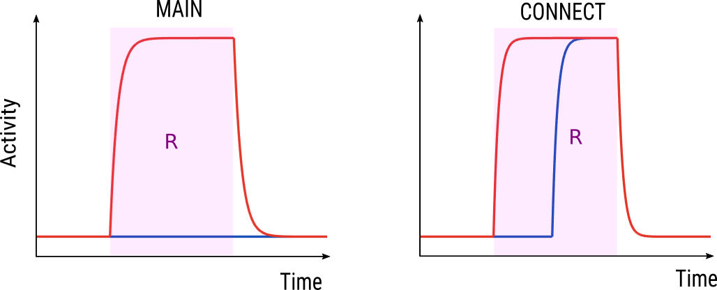
Figure 7: Example dynamics of the $u_{A}$ (red) and $u_{B}$ (blue) variables for MAIN and CONNECT states in an interval $R\in\Phi$. The left panel shows a MAIN state for which the A unit is OFF in $R$, while the B unit turns ON at time $t^{*}\!=\!\min(R)$. The right panel shows a CONNECT state for which the A unit turns ON at some time $t^{*}\!>\!\min(R)$, while the B unit turns ON at time $\min(R)$.

Remark 6.1.

MAIN states are either ON or OFF during any interval $R\in\Phi$, except (possibly) for a negligible interval of length $\sim 0$. Indeed due to differential convergence (Section 4.2) one unit may turn ON at $\alpha$ following an infinitesimally small delay $\delta\sim\tau$, where $\delta$ is given by equation 9.

6.1 Classification of MAIN and CONNECT states - Matrix form

The results reported in the previous section constraint the possible dynamics during each active tone interval $R\in\Phi$. In this section we use these results to propose a classification of MAIN and CONNECT states based on their dynamics during these intervals and define the existence conditions for these states.

Due to lemmas 3, 4 and 5 the units of any state must be OFF at the start $R$ (orbits $(u_{A},u_{B})$ always start from $(0,0)$ at time $\alpha$), may turn ON at most once in $R$ and, if this occurs, it must remain ON until the end of $R$. Thus we have three possibilities: (1) both units are OFF in $R$, (2) only one unit turns ON once in $R$ or (3) both units turn ON once in $R$. These possibilities guarantee that any state in the network can be classified as MAIN or CONNECT. We note that condition ($U_{1}$) guarantees that (1) cannot occur $\forall R\in\Phi$, or $(0,0,0,0)$ would be an equilibria. Let us define the total inputs to the units for the A and B active tone intervals as a function of the synaptic quantity $s$:

$$f(s)\!=\!\begin{cases}c\!-\!bs,&\mbox{if }R\!=\!I_{A}^{k}\\ d\!-\!bs,&\mbox{if }R\!=\!I_{B}^{k}\end{cases},\quad g(s)\!=\!\begin{cases}d\!-\!bs,&\mbox{if }R\!=\!I_{A}^{k}\\ c\!-\!bs,&\mbox{if }R\!=\!I_{B}^{k}\end{cases}$$ (10)

Classification of MAIN states. From the considerations given above the units’ dynamics in $R\!=\![\alpha,\beta]$ of any MAIN state is completely determined on the fast time scale at times $\alpha$ and $\beta$. Each unit can either turn ON at time $\alpha$ or be OFF at time $\beta$, depending on the system’s parameters and on the following quantities:

$$\quad\underline{s}_{A}\!=\!s_{A}(\alpha\!-\!D),\quad\bar{s}_{A}\!=\!s_{A}(\beta\!-\!D),\quad\underline{s}_{B}\!=\!s_{B}(\alpha\!-\!D),\quad\bar{s}_{B}\!=\!s_{B}(\beta\!-\!D)$$

Following the fixed point analyses we consider three conditions (summarized in Table 2):

• Both units turn ON at time $\alpha$. This is equivalent to $(1,1)$ being the only equilibrium for the fast subsystem at time $\alpha$, which may occur under the conditions $M_{1-3}$. In summary, for case $M_{1}$ both units instantaneously turn ON at time $\alpha$. For case $M_{2}$ ($M_{3}$) unit B (A) turns ON after A (B) of an infinitesimal delay $\delta\sim\tau$ (see Section 4.2).

• One unit turns ON at time $\alpha$ and the other unit is OFF at time $\beta$ - this corresponds to states satisfying one of conditions $M_{4-5}$. For case $M_{4}$ ($M_{5}$) A(B) turns ON at $\alpha$ and B(A) is OFF at $\beta$. Indeed $(1,0)$ ($(0,1)$) is the only stable equilibrium of the subsystem at times $\alpha$ and $\beta$, and thus $\forall t\in R$ due to Lemma 5.

• A and B are OFF at time $\beta$ - it occurs when $(0,0)$ is the only stable equilibrium of the fast subsystem at time $\beta$, thus satisfying condition $M_{6}$.

$M_{1}$	$M_{2}$	$M_{3}$	$M_{4}$	$M_{5}$	$\quad M_{6}$
$\begin{aligned} f(\underline{s}_{B})\!&\geq\!\theta\\ g(\underline{s}_{A})\!&\geq\!\theta\end{aligned}$	$\begin{aligned} g(\underline{s}_{A})\!&<\!\theta\\ f(\underline{s}_{B})\!&\geq\!\theta\\ a\!+\!g(\underline{s}_{A})\!&\geq\!\theta\end{aligned}$	$\begin{aligned} f(\underline{s}_{B})\!&<\!\theta\\ g(\underline{s}_{A})\!&\geq\!\theta\\ a\!+\!f(\underline{s}_{B})\!&\geq\!\theta\end{aligned}$	$\begin{aligned} f(\underline{s}_{B})\!&\geq\!\theta\\ a\!+\!g(\bar{s}_{A})\!&<\!\theta\end{aligned}$	$\begin{aligned} g(\underline{s}_{A})\!&\geq\!\theta\\ a\!+\!f(\bar{s}_{B})\!&<\!\theta\end{aligned}$	$\begin{aligned} g(\bar{s}_{A})\!&<\!\theta\\ f(\bar{s}_{B})\!&<\!\theta\end{aligned}$

Table 2: Existence conditions for MAIN states in an interval $R\in\Phi$

Figure 8 shows the time histories of the MAIN states satisfying conditions $M_{1-5}$ in an interval $R\in\Phi$ ($M_{6}$ has been omitted since both units are inactive). Overall, this analysis proves that for a fixed interval $R\in\Phi$ any MAIN state of system 1 satisfies only one of the above conditions $M_{1-6}$, and that any pair of MAIN states satisfying the same condition follow exactly the same dynamics in $R$. We can therefore define the dynamics of any MAIN state during any interval $R\in\Phi$ as follows.

Definition 6.2 (MAIN classification).

We define the set of MAIN states in $R\in\Phi$ as $M_{R}=\{s=s(t)\mbox{ solutions of \ref{model} satisfying one of conditions }M_{1-6}\mbox{ in }R\}$

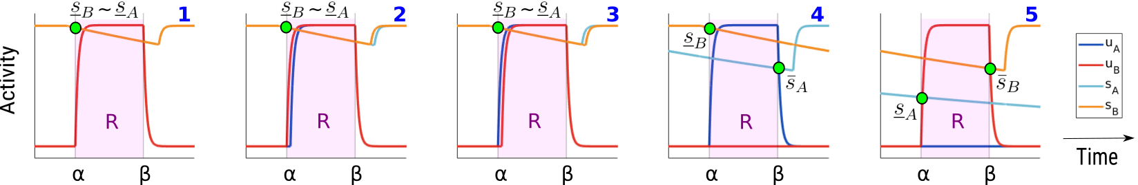
Figure 8: Example dynamics of a MAIN state satisfying condition $M_{1-5}$ in $R\in\Phi$.

In next Theorem we construct a binary matrix representation for MAIN states defined by their existence conditions. This tool will enable us to define the existence conditions for $2T\!R$-periodic states and to rule out impossible ones (see Theorem 9).

Theorem 6.

Let $R\in\Phi$. There is an injective map ρ^R :M_R →B(2,2) ,  s ↦V = [xAyAxByB] with entries defined by

$$x_{A}\!=\!H(f(\underline{s}_{B})),\;x_{B}\!=\!H(g(\underline{s}_{A})),\;y_{A}\!=\!\begin{cases}1&\textup{if }ax_{B}\!+\!f(\underline{s}_{B})\!\geq\!\theta\\ 0&\textup{if }ax_{B}\!+\!f(\bar{s}_{B})\!<\!\theta\end{cases},\;y_{B}\!=\!\begin{cases}1&\textup{if }ax_{A}\!+\!g(\underline{s}_{A})\!\geq\!\theta\\ 0&\textup{if }ax_{A}\!+\!g(\bar{s}_{A})\!<\!\theta\end{cases}$$ (11)

Moreover:

$$\textup{Im}(\rho^{R})=\Omega\stackrel{{\scriptstyle{\mbox{\footnotesize{def}}}}}{{=}}\{V=\rho^{R}(s):x_{A}\leq y_{A},\>x_{B}\leq y_{B},\>x_{A}=x_{B}=0\Rightarrow y_{A}=y_{B}=0\}$$ (12)

Proof.

A necessary condition for $\rho^{R}$ to be well defined is that $y_{A}$ and $y_{B}$ cannot be simultaneously equal to $0$ and $1$ (i.e. that both inequalities in their definition are not simultaneously satisfied). Due to the decay of the delayed synaptic variables in $R$ (Lemma 4) we have $\underline{s}_{B}\!\geq\!\bar{s}_{B}$. Moreover, since $f$ and $g$ are monotonically increasing, we have

$$f(\underline{s}_{B})\!\leq\!f(\bar{s}_{B})\quad\mbox{and}\quad g(\underline{s}_{B})\!\leq\!g(\bar{s}_{B})$$ (13)

Which proves that $y_{A}$ is exclusively equal to $0$ or $1$ (analogously for $y_{B}$).

Next, we notice that any matrix $V\!=\!\rho^{R}(s)$ satisfies the following:

$$x_{A}\leq y_{A},\quad x_{B}\leq y_{B},\quad x_{A}=x_{B}=0\Rightarrow y_{A}=y_{B}=0$$ (14)

We prove the first inequality $x_{A}\leq y_{A}$ ($x_{B}\leq y_{B}$ is analogous). WLOG we assume $x_{A}\!=1$, and therefore $f(\underline{s}_{B})\!\geq\!\theta$. Since $a\!\geq\!0$ and $x_{B}\!\geq\!0$ we have $ax_{B}\!+\!f(\underline{s}_{B})\!\geq\!f(\underline{s}_{B})\!\geq\!\theta$, thus implying $y_{A}\!=\!1$. The final part holds because, given $x_{A}\!=\!x_{B}\!=\!0$, we have $ax_{B}\!+\!f(\bar{s}_{B})\!\leq\!f(\underline{s}_{B})\!<\!\theta,\quad ax_{A}\!+\!g(\bar{s}_{A})\!\leq\!g(\underline{s}_{A})\!<\!\theta$.

From conditions 13 and 14 it is easily checked that each element $s\in M_{R}$ satisfying condition $M_{i}$ has one of the following images $\rho^{R}(s)$:

$$(M_{1})\;\begin{bmatrix}1&1\\ 1&1\end{bmatrix},\;(M_{2})\;\begin{bmatrix}1&1\\ 0&1\end{bmatrix},\;(M_{3})\;\begin{bmatrix}0&1\\ 1&1\end{bmatrix},\;(M_{4})\;\begin{bmatrix}1&1\\ 0&0\end{bmatrix},\;(M_{5})\;\begin{bmatrix}0&0\\ 1&1\end{bmatrix},\;(M_{6})\;\begin{bmatrix}0&0\\ 0&0\end{bmatrix}$$

Since any MAIN state has a distinct image, $\rho^{R}$ is well defined, injective, and $|Im(\rho^{R})|\!=\!6$. Given that the total number of matrices $V\in B(2,2)$ satisfying conditions 14 are precisely 6 (no other matrix is possible), we have $Im(\rho^{R})\!=\!\Omega$ ∎

Classification of CONNECT states. Our classification and matrix form of CONNECT states follows analogously from that of MAIN states described previously. We recall that in such states at least one unit turns ON at some time in an active tone interval $R\!=\![\alpha,\beta]$. There are three cases to consider:

1. Unit A(B) turns ON at time $\alpha$ and B(A) turns ON at time $t^{*}$, $\exists t^{*}\in(\alpha,\beta]$.

2. Unit A(B) is OFF at time $\beta$ and B(A) turns ON at time $t^{*}$, $\exists t^{*}\in(\alpha,\beta]$.

3. $\exists t^{*},s^{*}\in(\alpha,\beta]$ times when the A and B unit turns ON.

These lead to the conditions in Table 3, which are explained in the Supplementary Material LABEL:connect_appendix. Case 1. lead to the conditions $C_{1-2}$, cases 2. lead to the conditions $C_{3-4}$, while case 3. leads to two possibilities depending on if A turns ON before or after B: $C_{5}^{1}$ and $C_{5}^{2}$. For simplicity do not distinguish between these cases and define ($C_{5}$) as referring to either condition. This leads to the following definition.

$C_{1}$	$C_{2}$	$C_{3}$	$C_{4}$	$C_{5}^{1}$	$\quad\quad C_{5}^{2}$
$\begin{aligned} f(\underline{s}_{B})\!&\geq\!\theta\\ a\!+\!g(\underline{s}_{A})\!&<\!\theta\\ a\!+\!g(\bar{s}_{A})\!&\geq\!\theta\end{aligned}$	$\begin{aligned} g(\underline{s}_{A})\!&\geq\!\theta\\ a\!+\!f(\underline{s}_{B})\!&<\!\theta\\ a\!+\!f(\bar{s}_{B})\!&\geq\!\theta\end{aligned}$	$\begin{aligned} g(\underline{s}_{A})\!&<\!\theta\\ g(\bar{s}_{A})\!&\geq\!\theta\\ a\!+\!f(\bar{s}_{B})\!&<\!\theta\end{aligned}$	$\begin{aligned} f(\underline{s}_{B})\!&<\!\theta\\ f(\bar{s}_{B})\!&\geq\!\theta\\ a\!+\!g(\bar{s}_{A})\!&<\!\theta\end{aligned}$	$\begin{aligned} t^{*}\!&\leq\!s^{*}\\ f(\underline{s}_{B})\!&<\!\theta\\ f(\bar{s}_{B})\!&\geq\!\theta\\ a\!+\!g(\bar{s}_{B})\!&\geq\!\theta\end{aligned}$	$\begin{aligned} t^{*}\!&>\!s^{*}\\ g(\underline{s}_{A})\!&<\!\theta\\ g(\bar{s}_{A})\!&\geq\!\theta\\ a\!+\!f(\bar{s}_{A})\!&\geq\!\theta\end{aligned}$

Table 3: Existence conditions for CONNECT states in an interval $R\in\Phi$

Definition 6.3 (CONNECT classification).

We define the set of CONNECT states in $R\in\Phi$ as $C_{R}=\{s=s(t)\mbox{ solutions of \ref{model} satisfying one of conditions }C_{1-5}\mbox{ in }R\}$.

Similar to MAIN states, the existence conditions for each CONNECT state in $R$ can equivalently be expressed using a binary matrix $W\in B(2,3)$.

Theorem 7.

Set $R\in\Phi$. There is an injective map: φ^R:C_R →B(2,3) ,  s ↦W = [xAyAzAxByBzB] With entries defined by:

$$\begin{split}x_{A}\!&=\!H(f(\underline{s}_{B})),\>y_{A}\!=\!H(ax_{B}\!+\!f(\underline{s}_{B})),\>z_{A}\!=\!H(a\!+\!f(\bar{s}_{B}))\\ x_{B}\!&=\!H(g(\underline{s}_{A})),\>y_{B}\!=\!H(ax_{A}\!+\!g(\underline{s}_{A})),\>z_{B}\!=\!H(a\!+\!g(\bar{s}_{A}))\end{split}$$ (15)

And we have: Im(φ^R)​=​ { W : x_A ​≤​ y_A ​≤​ z_A, x_B ​≤​ y_B ​≤​ z_B, x_A​=​x_B​=​0 ⇒y_A​=​y_B​=​0, y_A​¡​z_A or y_B​¡​z_B }

The proof of this theorem is similar to the one of Theorem 6 and is given in the Supplementary Material LABEL:appendix_CONN_matr. As shown in this proof, each CONNECT state satisfying one of conditions $C_{1-5}$ has a corresponding image $\varphi^{R}(s)$ shown below.

$$(C_{1})\;\begin{bmatrix}1&1&1\\ 0&0&1\end{bmatrix}\quad(C_{2})\;\begin{bmatrix}0&0&1\\ 1&1&1\end{bmatrix}\quad(C_{3})\;\begin{bmatrix}0&0&0\\ 0&0&1\end{bmatrix}\quad(C_{4})\;\begin{bmatrix}0&0&1\\ 0&0&0\end{bmatrix}\quad(C_{5})\;\begin{bmatrix}0&0&1\\ 0&0&1\end{bmatrix}\quad$$

The previous two theorems naturally lead to the definition of the matrix form of the MAIN and CONNECT states in each interval $R\in\Phi$.

Definition 6.4 (Matrix form).

Let $R\in\Phi$ be an active tone interval:

• The matrix form of a MAIN state $s\in M_{R}$ is $V\!=\!\rho^{R}(s)$ defined by 11.

• The matrix form of a CONNECT state $s\in C_{R}$ is $W\!=\!\varphi^{R}(s)$ defined by 15.

Remark 6.2 (Visualisation via the Matrix form).

The first (second) row of the matrix form of each MAIN state provide an intuitive visualization of its A (B) units’ dynamics in $R$. Indeed, given $\delta$ as defined in Section 4.2 we may subdivide $R$ into $R=[\alpha,\alpha\!+\!\delta]\cup[\alpha\!+\!\delta,\beta]$. The dynamics of the A unit at time $\alpha$ is given by $x_{A}$. If $x_{A}\!=\!1$ the A unit turns ON at time $\alpha$ and remains ON in $(\alpha,\beta]$. If $x_{A}=0$ and $y_{A}\!=\!1$ the A unit is OFF at time $\alpha$, turns ON at time $\alpha+\delta$ and remains ON in $(\alpha+\delta,\beta]$. If $y_{A}\!=\!0$ (which implies $x_{A}\!=\!0$) the A unit is OFF $\forall t\in R$. Similar considerations hold for the B unit.

Similarly, the dynamics of the A (B) unit in $R$ of a CONNECT state is represented by the first (second) row of its matrix form. For example, for the state defined by condition $C_{2}$ unit A turns ON at some time $t^{*}\in(\alpha,\beta]$, while unit B turns ON at time $\alpha$. Given $\delta$ as defined in Section 4.2, we may subdivide $R$ into $R=[\alpha,\alpha\!+\!\delta]\cup[\alpha\!+\!\delta,t^{*}]\cup[t^{*},\beta]$. From conditions $C_{2}$ we have $y_{A}\!=\!0$ (which implies $x_{A}\!=\!0$) and $z_{A}\!=\!1$. Thus A is OFF during $[\alpha,\alpha+\delta]$ and $[\alpha\!+\!\delta,t^{*}]$, turns ON at time $t^{*}$ and remains ON in $[t^{*},\beta]$. Since $x_{B}\!=\!1$ (which implies $y_{B}\!=\!z_{B}\!=\!1$), the B unit turns ON at time $\alpha$ and remains ON in $[\alpha,\beta]$.

Remark 6.3 (Matrix form extension for MAIN states).

We showed that MAIN (CONNECT) states in an interval $R\in\Phi$ can be represented using a $2\times 2$ ($2\times 3$) binary matrix. However, MAIN states can also be equivalently represented using the same $2\times 3$ matrix form $W$ defined for CONNECT states in the previous theorem, by replacing the definition of $z_{A}$ and $z_{B}$ with $z_{A}\!=\!H(ay_{B}\!+\!f(\bar{s}_{B}))$ and $z_{B}\!=\!H(ay_{A}\!+\!g(\bar{s}_{A}))$. One can check that each existence condition $M_{1-6}$ given in 15 defines one of the following $2\times 3$ matrices:

$$(M_{1})\begin{bmatrix}1&1&1\\ 1&1&1\end{bmatrix}(M_{2})\begin{bmatrix}1&1&1\\ 0&1&1\end{bmatrix}(M_{3})\begin{bmatrix}0&1&1\\ 1&1&1\end{bmatrix}(M_{4})\begin{bmatrix}1&1&1\\ 0&0&0\end{bmatrix}(M_{5})\begin{bmatrix}0&0&0\\ 1&1&1\end{bmatrix}(M_{6})\begin{bmatrix}0&0&0\\ 0&0&0\end{bmatrix}$$

This result guarantees that we can represent all the states in the system using a general $2\times 3$ matrix form (used in Section 7).

So far we have shown the existence conditions for MAIN and CONNECT states in any active tone interval $R$. The following lemma regards the conditions for which LONG states can occur. This will enable us to complete the existence conditions for all states outside the active tone intervals.

Lemma 8 (LONG conditions).

A state is LONG if and only if $\exists R=[\alpha,\beta]\in\Phi$:

1. A and B turn ON at times $t^{*}_{A}$ and $t^{*}_{B}\in R$, respectively.

2. $a\!-\!bs_{A}(\beta\!-\!D)\geq\theta$ and $a\!-\!bs_{B}(\beta\!-\!D)\geq\theta$.

Moreover, both units are ON in $[\beta,t^{*}\!+\!D]$, turn OFF at time $t^{*}\!+\!D$, and are OFF in $(t^{*}\!+\!D,t_{up}]$, where $t^{*}=\min\{t^{*}_{A},t^{*}_{B}\}\quad\mbox{and}$ and $t_{up}=\min_{s\in I}\{s>t\}$.

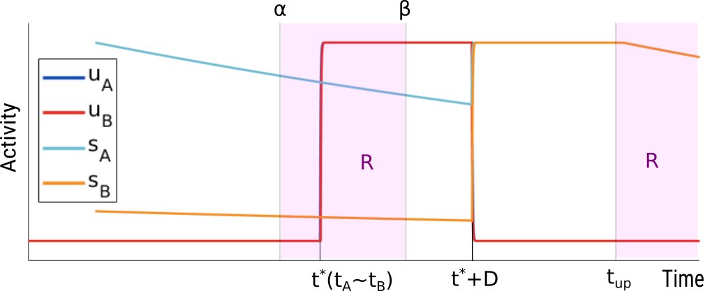
Figure 9: Example dynamics of a LONG state showing quantities used in Lemma 8.

The proof of this lemma is given in the Supplementary Material LABEL:appendix_LONG_thm. The idea of the proof is sketched in Figure 9. Both units of a LONG stats must be ON at time $\beta$ due to Theorem 1, which proves to 2. Furthermore, since both synaptic variables are monotonically decaying in the interval $[\alpha,t^{*}\!+\!D]$ this activity must persist until time $t^{*}\!+\!D$, when one of these variables (or both) jump to 1.

7 2TR-periodic states

In the previous section we classified network states in a generic active tone interval. In this section we use this analysis to study $2T\!R$-periodic states under the conditions $D\!>\!TD$ and $T\!D\!+\!D\!<\!T\!R$. We analytically derive the parameter conditions leading to the existence of all $2T\!R$-periodic states in the system and use the matrix form to rule out which states cannot exist.

Definition 7.1.

A state $\psi\!=\!\psi(t)\!=\!(u_{A}(t),u_{B}(t),s_{A}(t),s_{B}(t))$ is $2T\!R$-periodic if $\psi(t\!+\!2T\!R)=\psi(t)$, $\forall t\in\mathbb{R}$. We call $SM$ and $LM$ ($SC$ and $LC$) the sets of $2T\!R$-periodic MAIN (CONNECT) states of the SHORT and LONG type, respectively.

Before analyzing these states it is important to first assess the model’s symmetry.

Remark 7.1 ($\mathbb{Z}_{2}$ symmetry).

System 1 is symmetric under a transformation swapping the A and B indexes in system 1 and by applying the time shift $T\!R$ to the active tone input functions. Indeed let us rewrite the model as a general non-autonomous dynamical system ˙v(t)=z(v(t),i_A(t),i_B(t)),  v​=​(u_A,u_B,s_A,s_B) Now consider the map $\kappa$ whose action swaps the A and B indices of all variables, defined as κ: v=(u_A,u_B,s_A,s_B,i_A,i_B) ↦(u_B,u_A,s_B,s_A,i_B,i_A) Since $i_{A}(t\!+\!T\!R)\!=\!i_{B}(t)$ and $i_{B}(t\!+\!T\!R)\!=\!i_{A}(t)$, $\forall t\in\mathbb{R}$, we have κ(z(v(t),i_A(t),i_B(t))) ​=​ z(κ(v(t​+​T​R),i_B(t​+​T​R),i_A(t​+​T​R))), which proves the model is symmetric under the transformation $\kappa$ time shifted by $T\!R$. Given that no symmetric transformation other than $\kappa$ and the identity exist, the system is $\mathbb{Z}_{2}$-equivariant. Thus, given a periodic solution $v(t)$ with period $T$, its $\kappa$-conjugate cycle $\kappa(v(t\!+\!TR))$ must also be a solution with equal period (asymmetric cycle), except in the case that $v(t)\!=\!\kappa(v(t)),\,\forall t\!\in\![0,T]$ (symmetric cycle). Asymmetric cycles always exist in pairs: the cycle and its conjugate. We note that in-phase and anti-phase limit cycles with period $2T\!R$ are both symmetric cycles.

To study $T\!R$-periodic states we can replace the set of active tone intervals $I$ with: I=I_1 ∪I_2=[0,T​D] ∪[T​R,T​R​+​T​D] As shown in the previous section, for any state $\psi\in SM$ the activities of both units during each interval $I_{i}$, with $i=1,2$, can be represented by a matrix $V_{i}$. This matrix uniquely depends on the values of the delayed synaptic variables at times $\alpha_{i}=(i\!-\!1)T\!R$ and $\beta_{i}=(i\!-\!1)T\!R\!+\!T\!D$. More precisely, in equations 11 we must substitute $\underline{s}_{A}$ with $s^{i-}_{A}$, $\bar{s}_{A}$ with $s^{i+}_{A}$, $\underline{s}_{B}$ with $s^{i-}_{B}$ and $\bar{s}_{B}$ with $s^{i+}_{B}$, where:

$$s^{i-}_{A}\!=\!s_{A}(\alpha_{i}-D),\quad s^{i-}_{B}\!=\!s_{B}(\alpha_{i}\!-\!D),\quad s^{i+}_{A}\!=\!s_{A}(\beta_{i}\!-\!D),\quad s^{i+}_{B}\!=\!s_{B}(\beta_{i}\!-\!D$$ (16)

7.1 SHORT states

It turns out (see Theorem below) that for SHORT MAIN and CONNECT states these values depend on the following quantities, as stated in the next Theorem.

$$N^{-}\!=\!e^{-(TR\!-\!TD\!-\!D)/\tau_{i}},\;N^{+}=e^{-(TR\!-\!D)/\tau_{i}},\;M^{-}\!=\!e^{-(2TR\!-\!TD\!-\!D)/\tau_{i}},\;M^{+}=e^{-(2TR\!-\!D)/\tau_{i}}$$ (17)

We note that $N^{-}\!\geq\!N^{+}\!\geq\!M^{-}\!\geq\!M^{+}$. The dependence of the synaptic variables on these quantities is crucial, because it guarantees that the existence conditions shown in Table 2 depend uniquely on the model parameters for $2T\!R$-periodic states.

Theorem 9.

There is an injective map ρ:SM →B(2,4) ,  ψ↦V = [[c—c] V1V2] = [[cc—cc] xA1yA1xA2yA2xB1yB1xB2yB2]

Where $V_{1}$ ($V_{2}$) is the matrix form of $\psi$ in $I_{1}$ ($I_{2}$) defined by 11, and:

$$s_{B}^{i\pm}\!=\!N^{\pm}y_{B}^{j}\!+\!M^{\pm}(1-y_{B}^{j})y_{B}^{i},\quad s_{A}^{i\pm}\!=\!N^{\pm}y_{A}^{j}\!+\!M^{\pm}(1-y_{A}^{j})y_{A}^{i},\quad\forall j\!=\!1,2,j\!\neq\!i$$ (18)

In addition, Im(ρ)=Ω=def{V = [[c—c] V1V2] : V_1 ∈Im(ρ^I_1), V_2 ∈Im(ρ^I_1) satisfying 1-4 below }

1. $y_{A}^{1}=y_{B}^{2}=1\Rightarrow x_{A}^{1}=x_{B}^{2}$ and $y_{A}^{2}=y_{B}^{1}=1\Rightarrow x_{A}^{2}=x_{B}^{1}$

2. $y_{B}^{1}=y_{B}^{2}\Rightarrow x_{A}^{1}\geq x_{A}^{2}$ and $y_{A}^{1}=y_{A}^{2}\Rightarrow x_{B}^{2}\geq x_{B}^{1}$

3. $y_{A}^{2}=1\Rightarrow x_{B}^{1}\leq r$ and $y_{B}^{1}=1\Rightarrow x_{A}^{2}\leq r$, for any entry $r$ in $V$

4. $y_{A}^{2}=y_{B}^{2}$, $y_{A}^{1}=y_{B}^{1}\Rightarrow x_{A}^{1}\geq x_{B}^{1}$ and $x_{B}^{2}\geq x_{A}^{2}$

Proof.

The proofs of equations 18 and of conditions 1-4 is given in the Supplementary Material LABEL:appendix_thm_MAIN_R. The validity of these conditions implies $Im(\rho)\subseteq\Omega$. In the next paragraph we will prove that $Im(\rho)\!=\!\Omega$. Assume for now this to be true. The definition of the entries of $V$ and identities 18 give multiple necessary and sufficient conditions for determining the dynamics of the corresponding MAIN state $\psi\!=\!\rho^{-1}(V)$ in the intervals $I_{1}$ and $I_{2}$, respectively. Due to the model’s symmetry (Remark 7.1) $V$ is the image of either a symmetrical or an asymmetrical state $\psi$. In the latter case, there exists a matrix $V^{\prime}\in\Omega$ for a state conjugate to $\psi$. One can easily show that $V^{\prime}$ is simply defined given $V$ by swapping the first (second) row of $V_{1}$ with the second (first) row of $V_{2}$. Notably, both $\psi$ and $\psi^{\prime}$, and thus also $V$ and $V^{\prime}$, exist under the same parameter conditions. The second rows of Table 4 shows all matrices $V\in\Omega$ that are an image of either of a symmetrical state or one of two conjugate states and their names (1st row). Given that $I$, $AP$ and $ID$ are the only symmetrical cycles (in-phase and anti-phase), from Remark 7.1 all other states have another existing conjugate cycles that exists under the same conditions.

-	$S$	$SB$	$SD$	$AP$	$AS$	$ASD$	$I$	$ID$	$\quad IB$
Matrix	$\begin{array}[]{cccc}1100\\ 0000\\ \end{array}$	$\begin{array}[]{cccc}1100\\ 1100\\ \end{array}$	$\begin{array}[]{cccc}1100\\ 0100\\ \end{array}$	$\begin{array}[]{cccc}1100\\ 0011\\ \end{array}$	$\begin{array}[]{cccc}1111\\ 0011\\ \end{array}$	$\begin{array}[]{cccc}1101\\ 0011\\ \end{array}$	$\begin{array}[]{cccc}1111\\ 0000\\ \end{array}$	$\begin{array}[]{cccc}1101\\ 0111\\ \end{array}$	$\begin{array}[]{cccc}1111\\ 1111\\ \end{array}$
Conditions	$\begin{aligned} C_{1}\!&<\!\theta\\ C_{2}^{+}\!&<\!\theta\\ C_{3}^{+}\!&<\!\theta\end{aligned}$	$\begin{aligned} C_{3}^{+}\!&<\!\theta\\ C_{8}^{-}\!&\geq\!\theta\end{aligned}$	$\begin{aligned} C_{4}^{-}\!&\geq\!\theta\\ C_{2}^{-}\!&\geq\!\theta\\ C_{3}^{+}\!&<\!\theta\\ C_{8}^{-}\!&<\!\theta\end{aligned}$	$\begin{aligned} C_{2}^{+}\!&<\!\theta\\ C_{3}^{-}\!&\geq\!\theta\end{aligned}$	$\begin{aligned} C_{3}^{-}\!&\geq\!\theta\\ C_{5}^{+}\!&<\!\theta\\ C_{8}^{-}\!&\geq\!\theta\end{aligned}$	$\begin{aligned} C_{2}^{-}\!&\geq\!\theta\\ C_{3}^{-}\!&\geq\!\theta\\ C_{5}^{+}\!&<\!\theta\\ C_{8}^{-}\!&<\!\theta\end{aligned}$	$\begin{aligned} C_{1}\!&\geq\!\theta\\ C_{6}^{+}\!&<\!\theta\end{aligned}$	$\begin{aligned} C_{3}^{-}\!&\geq\!\theta\\ C_{5}^{-}\!&\geq\!\theta\\ C_{7}^{-}\!&<\!\theta\end{aligned}$	$\begin{aligned} C_{7}^{-}\!\geq\!\theta\end{aligned}$
Short	$-$	$C_{9}\!<\!\theta$	$C_{9}\!<\!\theta$	$-$	$\begin{aligned} C_{10}\!<\!\theta\end{aligned}$	$\begin{aligned} C_{10}\!<\!\theta\end{aligned}$	$-$	$\begin{aligned} C_{10}\!<\!\theta\end{aligned}$	$\begin{aligned} C_{10}\!<\!\theta\end{aligned}$

Table 4: Matrix form and existence conditions of all $2T\!R$-periodic SHORT MAIN states. Names (first row) were chosen following our proposed link between states and percepts in auditory streaming (see Section 3). Names starting with S correspond to segregation (no unit responds to both tones), I to integration (one unit responds to both tones, the other is inactive or responding to both tones, too) and AP to bistability (one unit responds to both tones, the other unit to every other tone). The letter D corresponds to states for which one units turns ON with a small delay after the other unit in one active tone interval. The letter B corresponds to states for which both units follow the same dynamics.

In the next part we define the conditions for existence of each of the states reported in the third row of Table 4, which are equivalent to the well-definedness conditions of the corresponding matrix form $V\in\Omega$. These conditions depend on:

$$\begin{split}C_{1}\!=\!d,\quad C_{2}^{\pm}\!=\!a\!-\!bM^{\pm}\!+\!d,\quad C_{3}^{\pm}\!=\!\!c\!-\!bN^{\pm},\quad C_{4}^{\pm}\!=\!\!c\!-\!bM^{\pm}\!,\quad C_{5}^{\pm}\!=\!a\!-\!bN^{\pm}\!+\!d,\quad\\ C_{6}^{\pm}\!=\!a\!-\!bN^{\pm}\!+\!c,\quad C_{7}^{\pm}\!=\!\!d\!-\!bN^{\pm}\!,\quad C_{8}^{\pm}\!=\!\!d\!-\!bM^{\pm}\!,\quad C_{9}\!=\!\!a-\!bM^{+}\quad C_{10}\!=\!a\!-\!bN^{+}\end{split}$$ (19)

One determine conditions for the well-definiteness of each matrix $V\in\Omega$ from the definitions of the entries of $V_{1}$ and $V_{2}$ given in 14 and using formulas 18. Notably, all the existence conditions uniquely depend on the system’s parameters. When determining these conditions one notices that many of them are redundant, and can be simplified using the following properties: $N^{-}\!\geq\!N^{+}\!\geq\!M^{-}\!\geq\!M^{+}$, $d\!\leq\!c$ and $a\geq 0$. In the next paragraph, we show one example ($AS$) and leave the remaining for the reader to prove. The names and the sets of inequalities defining each state is reported in the middle row of Table 4. We note such inequalities are well-posed, meaning that there is a region of parameter where they are all satisfied. This effectively proves that for each matrix $V\in\Omega$ there exists a state $\psi\!=\!\rho^{-1}(V)\in SM$ whose dynamics during intervals $I_{1}$ and $I_{2}$ are defined by the entries of $V$.

We now prove that $AS$’ existence conditions in Table 4 are well-defined, that is:

$$V_{AS}=\begin{bmatrix}[cc|cc]1&1&1&1\\ 0&0&1&1\end{bmatrix}\quad\Leftrightarrow\quad C_{3}^{-}\!\geq\!\theta,\quad C_{5}^{+}\!<\!\theta,\quad C_{8}^{-}\!\geq\!\theta.\quad$$ (20)

From condition (1) in 9 we have that x_A^1​=​1 ⇒y_A^1​=​1,  x_A^2​=​1 ⇒y_A^2​=​1,  x_B^2​=​1 ⇒y_B^2​=​1,  y_B^1​=​0 ⇒x_B^1​=​0, This obviously leads to the follow equivalence

$$V_{AS}=\begin{bmatrix}[cc|cc]1&1&1&1\\ 0&0&1&1\end{bmatrix}\quad\Leftrightarrow\quad x_{A}^{1}\!=\!1,\quad x_{B}^{2}\!=\!1,\quad x_{A}^{2}\!=\!1,\quad y_{B}^{1}\!=\!0.$$

Using the definition of the entries defined in 14 and the identities for the synaptic quantities given in equations 18 we observe the following:

1. $y_{A}^{1}\!=\!1\left(y_{B}^{2}\!=\!1\right)\Rightarrow s_{A}^{2-}\!=\!N^{-}\left(s_{B}^{1-}\!=\!N^{-}\right)$, which implies $x_{B}^{2}\!=\!x_{A}^{1}\!=\!H(c\!-\!bN^{-})$

2. $y_{B}^{1}\!=\!0\mbox{ and }y_{B}^{2}\!=\!1\Rightarrow s_{B}^{2-}\!=\!M^{-}$. From this $x_{A}^{2}\!=\!H(d\!-\!bM^{-})$

3. $y_{A}^{2}\!=\!1\Rightarrow s_{A}^{1+}\!=\!N^{+}$. This and $y_{B}^{1}\!=\!0$ give $y_{B}^{1}\!=\!H(a\!+\!d\!-\!bN^{+})$

Overall, from the cases (1-3) above we obtain

$$x_{A}^{1}\!=\!1,x_{B}^{2}\!=\!1\Leftrightarrow C_{3}^{-}\!\geq\!\theta,\quad x_{A}^{2}\!=\!1\Leftrightarrow C_{8}^{-}\!\geq\!\theta,\quad y_{B}^{1}\!=\!0\Leftrightarrow C_{5}^{+}\!<\!\theta.$$

This completes the proof for both the claim 20 and the Theorem. ∎

Remark 7.2 (Conditions $C_{9}$ and $C_{10}$).

The middle row of Table 4 shows existence condition that determine the dynamics of each state in the intervals $I_{1}$ and $I_{2}$. However, they do not guarantee these states being OFF in $[0,2T\!R]\!-\!I$ (ie being SHORT). From Lemma 8 there are two cases to consider:

1. If both units turn ON during interval $I_{1}$ or $I_{2}$ one must guarantee that the second condition of Lemma 8 is not valid in each interval $I=[\alpha,\beta]=I_{1}$ or $I_{2}$ during which this occurs, one must impose

   $$\min\{a\!-\!bs_{A}(\beta\!-\!D),a\!-\!bs_{B}(\beta\!-\!D)\}\!<\!\theta$$ (21)

   This condition is expressed differently for each MAIN state in Table 4:

   • For $SB$ and $SD$ both units turn ON during interval $I_{1}$ ($I_{2}$ for their conjugate state). Equations 18 lead to $s_{A}(T\!D\!-\!D)\!=\!s_{B}(T\!D\!-\!D)=M^{+}$. Thus condition $C_{9}\!<\!0$ guarantees that inequalities 21 are satisfied.

   • For $AS$ and $ASD$ both units are ON during $I_{2}$ ($I_{1}$ for their conjugate state). To guarantee condition 21 at time $\beta\!=\!T\!R\!+\!T\!D$ one notices that equations 18 give $s_{A}(T\!R\!+T\!D\!-\!D)\!=N^{+}$ and $s_{B}(T\!R\!+T\!D\!-\!D)=M^{+}$. Thus, condition $C_{10}\!<\!0$ guarantees that condition 21 is satisfied.

   • For states $ID$ and $IB$ we notice that condition 21 is symmetrical on both intervals $I_{1}$ and $I_{2}$. Thus we may restrict the study on interval $I_{1}$. Similar to the two previous cases the application of equations 18 gives $s_{A}(T\!D\!-\!D)\!=\!s_{B}(T\!D\!-\!D)\!=\!N^{+}$. Thus we obtain $C_{10}\!<\!0$.

   The bottom row of Table 4 contains the additional conditions on $C_{9}$ and $C_{10}$ to be applied to each of the states analysed above.

2. If during both intervals $I_{1}$ and $I_{2}$ at least one unit is OFF the first condition of Lemma 8 is not satisfied, thus the state is SHORT with no extra conditions. These considerations hold for $S$, $AP$ and $I$.

Remark 7.3 (Table 4).

The conditions in the middle and bottom rows of Table 4 complete the existing conditions for all $2T\!R$-periodic SHORT MAIN states. Indeed these conditions covers all possible matrix forms and corresponding states. The middle row shows conditions determining the dynamics within in the intervals $I_{1}$ and $I_{2}$. The bottom row shows conditions that guarantee units to be OFF in $[0,2T\!R]\!-\!I$.

Figure 10A shows time histories for each $2T\!R$-periodic SHORT MAIN states in Table 4. We note that the conditions given in this table allow us to determine the regions where each of these states exists in the parameter space. To visualize 2-dimensional existence regions when varying pairs of model parameters we defined a new parameter $D\!F\in[0,1]$ and set $d\!=\!cD\!F$ ($D\!F$ is a scaling factor for the inputs from tonotopic locations). Figure 10B shows the two dimensional region of existence of states of each of these states at varying $DF$ and input strength $c$.

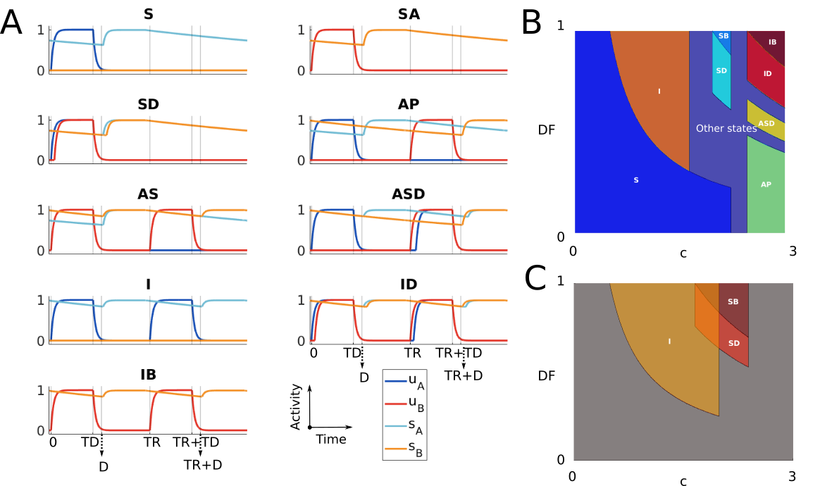
Figure 10: A. Time histories of $2T\!R$-periodic SHORT MAIN states B. Existence regions of states in A. when varying $DF$ and $c$. C. Existence regions for states $I$, $S\!B)$ and $S\!D$ at varying $c$ and $D\!F$. Parameters in B and C are $\tau_{i}\!=\!0.4$, $\theta\!=\!0.5$, and in B (C) $T\!D\!=\!0.03\,(0.005)$, $D\!=\!0.03\,(0.015)$, $P\!R\!=\!17\,(5)$, $a\!=\!0.6\,(0.4)$, $b\!=\!2\,(3)$.

From Table 4 we can establish the coexistence of MAIN states, as shown in the next theorem.

Theorem 10 (Multistability).

The state $I$ may coexist with $S\!B$ or $S\!D$. Any other pair of $2T\!R$-periodic SHORT MAIN states cannot coexist.

The proof of this theorem is in the Supplementary Material LABEL:multistability_appendix. Figure 10C shows a parameter regime show which states $I$ coexists with $S\!B$ and $S\!D$.

The analysis for $2T\!R$-periodic SHORT CONNECT states is similar to that of SHORT MAIN states, which we now summarize.

Theorem 11.

There is an injective map: φ:SC →B(2,6) ,  ψ↦W = [[c—c] W1W1] = [[ccc—ccc] xA1yA1zA1xA2yA2zA2xB1yB1zB1xB2yB2zB2] Where, for $i\!=\!1,2$, $W_{i}$ is the matrix forms of $\psi$ in $I_{i}$ defined in 15. Then: Im(φ) ​=​ {W​=​φ(ψ) , where W is one of the matrices shown in Table 5 }

$ZcS^{*}$	$ZcAP$	$ZcAS^{*}$	$ZcI$	$ScAS^{*}$	$SDcAS^{*}$	$ScSD^{*}$	$APcAS^{*}$	$APcI$
$\begin{array}[]{c}001000\\ 001000\\ \end{array}$	$\begin{array}[]{c}001000\\ 000001\\ \end{array}$	$\begin{array}[]{c}001001\\ 000001\\ \end{array}$	$\begin{array}[]{c}001001\\ 001001\\ \end{array}$	$\begin{array}[]{c}001111\\ 000001\\ \end{array}$	$\begin{array}[]{c}001111\\ 000011\\ \end{array}$	$\begin{array}[]{c}111000\\ 001000\\ \end{array}$	$\begin{array}[]{c}111001\\ 000111\\ \end{array}$	$\begin{array}[]{c}111001\\ 001111\\ \end{array}$

Table 5: Matrix form of $2T\!R$-periodic SHORT CONNECT states (* asymmetrical states). These states’ dynamics is connecting branches of pairs of MAIN states or the inactive state ($Z$). For example $ZcS$ connects the inactive state with one of the segregated states $S$, $SB$ or $SD$. The names chosen for CONNECT states (first row) contains the names of the two MAIN states separated by the letter c.

A complete version of this theorem (similar to Theorem 9) proving the existence conditions for all SHORT CONNECT states is in the Supplementary Material LABEL:appendix1. Table 5 shows names (first row) and matrix forms (second row) of all possible $2T\!R$-periodic SHORT CONNECT states. We omit time histories for these states because they can be visualized from their matrix form (see Remark 6.2).

7.2 LONG MAIN states

The analysis of LONG states is an extension of the SHORT states’ one. In this section we briefly report the main ideas, the details in the Supplementary Material LABEL:appendix2. The first step is to extend the matrix form definition to LONG states by including a last column in the matrix form of SHORT MAIN states. This new column is selected to satisfy the properties of LONG states described in Lemma 8. The matrix form for a state $\psi\in LM$ is the $2\times 6$ binary matrix $V$ defined as

$$V=\begin{bmatrix}[c|c||c|c]V_{1}&\vec{w}^{1}&V_{2}&\vec{w}^{2}\end{bmatrix}=\begin{bmatrix}[cc|c||cc|c]x_{A}^{1}&y_{A}^{1}&w^{1}&x_{A}^{2}&y_{A}^{2}&w^{2}\\ x_{B}^{1}&y_{B}^{1}&w^{1}&x_{B}^{2}&y_{B}^{2}&w^{2}\end{bmatrix}$$

Where $V_{1}$ and $V_{2}$ are the same matrix forms defined for MAIN SHORT states and the binary vectors $\vec{w}^{1}$ and $\vec{w}^{2}$ are defined by

$$w^{1}=H(ay_{A}^{1}-bs_{A}^{1+})H(ay_{B}^{1}-bs_{B}^{1+})\quad\mbox{and}\quad w^{2}=H(ay_{A}^{2}-bs_{A}^{2+})H(ay_{B}^{2}-bs_{B}^{2+}).$$ (22)

We remind the reader that $s_{A}^{1+}\!=\!s_{A}(T\!D\!-\!D)$, $s_{B}^{1+}\!=\!s_{B}(T\!D\!-\!D)$, $s_{A}^{2+}\!=\!s_{A}(T\!R\!+\!T\!D\!-\!D)$ and $s_{B}^{2+}\!=\!s_{B}(T\!R\!+\!T\!D\!-\!D)$. Using a similar proof as the one of Theorem 9 we can use the matrix form to define the existence conditions of the states and exclude impossible ones. Table 6 contains the names and matrix form of all the possible LONG MAIN states, and their existence conditions are reported in Table LABEL:tab:LM_SC_table_main.

$IL_{1}$	$IL_{2}^{*}$	$ASDL_{1}^{*}$	$ASL^{*}$	$SL^{*}$	$IDL_{1}$	$IDL_{2}^{*}$	$ASDL_{2}^{*}$	$SDL^{*}$
$\begin{array}[]{c}111111\\ 111111\\ \end{array}$	$\begin{array}[]{c}111110\\ 111110\\ \end{array}$	$\begin{array}[]{c}111010\\ 111110\\ \end{array}$	$\begin{array}[]{c}111000\\ 111110\\ \end{array}$	$\begin{array}[]{c}111000\\ 111000\\ \end{array}$	$\begin{array}[]{c}111011\\ 011111\\ \end{array}$	$\begin{array}[]{c}111010\\ 011110\\ \end{array}$	$\begin{array}[]{c}111000\\ 011110\\ \end{array}$	$\begin{array}[]{c}111000\\ 011000\\ \end{array}$

Table 6: Matrix form of the $2T\!R$-periodic LONG MAIN states (* asymmetrical states). Names (first row) are the same as the corresponding MAIN states, except from adding the final letter L, and an a subscript number to differentiate LONG states corresponding to the same MAIN state.

The existence conditions of SHORT CONNECT and LONG MAIN states can be visualized as a 2D parameter projection, similar to Figure 10B for SHORT MAIN states. Figure 11A,C show two examples when varying parameters $(c,D\!F)$, and the remaining parameters have been fixed to satisfy $T\!D\!<\!D$ and $T\!D\!+\!D\!<\!T\!R$. Panels A. and C. respectively show the existence regions for SHORT CONNECT and LONG MAIN states. In panel A. SHORT MAIN states are shown in dark blue to help the comparison with Figure 10B (same parameters). Figure 11B,D show time histories for the SHORT CONNECT state $APcAS$ and the LONG MAIN state $SDL$.

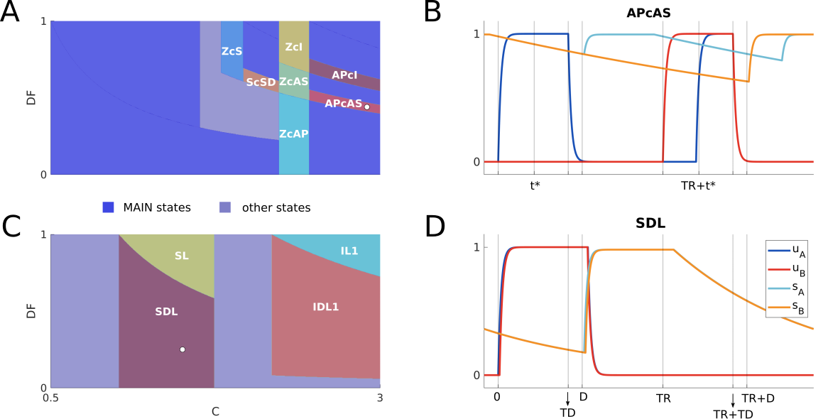
Figure 11: Visualization of SHORT CONNECT and LONG MAIN states. Panels A. and C. show regions of existence respectively for SHORT CONNECT and LONG MAIN states. SHORT MAIN states in panel A. are shown in dark blue. States that are neither SHORT MAIN, SHORT CONNECT or LONG MAIN are shown in light blue. For the same parameters as in A. and D., panels B. and D. respectively show example time histories for a SHORT CONNECT state ($APcAS$) and a LONG MAIN state ($SDL$) with fixed $(c,D\!F)$ shown by white dots in A. and D. In panel A. the parameters are the same as in Figure 10B. In panel C. parameters are the same as in A. except for $\tau_{i}\!=\!0.05$ and $a\!=\!2$.

Remark 7.4 (CONNECT states).

By comparing Figure 11A with Figure 10B (same parameters) we note that the union of the regions of existence of MAIN states is larger than the one of CONNECT states, hence why we call the first group MAIN. In addition SHORT CONNECT states connect branches of SHORT MAIN states, hence why we called them CONNECT (see Table 5).

7.2.1 Remaining states

As shown in the Section 7, $2T\!R$-periodic states can be SHORT MAIN ($SM$), SHORT CONNECT ($SC$), LONG MAIN ($LM$) or LONG CONNECT ($LC$) during each interval $I_{1}$ and $I_{2}$. We define $X|Y$ the set of states satisfying condition X during $I_{1}$ and Y during $I_{2}$, where $X,Y\in\{SM,SC,LM,LC\}$. In Section 7 we have the existence conditions of all possible states in some of these sets. More precisely:

• The analysis of $SM|SM$ is summarized in Table 4

• The analysis of $SC|SM$, $SM|SC$ and $SC|SC$ is summarized in Table 5

• The analysis of $LM|LM$, $SM|LM$ and $LM|SM$ is summarized in Table 6

The analysis of all remaining combinations of sets $X|Y$ are in the Supplementary Material LABEL:appendix3 and concludes the existence conditions for all $2T\!R$-periodic states.

8 Biologically relevant case: $2T\!R$-periodic states for $D\!\leq\!TD$

In this section we study model states and their link to auditory streaming under (1) $D\!\leq\!TD$ and (2) $T\!D\!+\!D\!<\!T\!R$. These inequalities are relevant to studying auditory streaming: condition (1) because delayed inhibition would be caused by factors that generate short delays, leading, condition (2) is guaranteed for the values of $T\!D$ and $T\!R$ typically tested in these experiments (further motivated in the Discussion).

By assuming that tonotopic inputs to the units are stronger than their mutual inhibition we derive analytically the existence conditions of all possible $2T\!R$-periodic states (Table 7 and 8). Overall, we find a total of 10 possible states (shown in Figure 12A). We link these states with the possible perceptual outcomes in the auditory streaming paradigm and find a qualitatively agreement between model and experiments when varying inputs’ parameters $df$ and $P\!R$ (Figure 12B and C). Furthermore, the states’ existence conditions let us formulate the coherence and fission boundaries separating the percepts as functions of $P\!R$ (Equations 25).

We now proceed to determine the detailed analysis of these $2T\!R$-periodic states. We consider active tone intervals $I\!=\!I_{1}\cup I_{2}$, where $I_{1}\!=\![0,T\!D]$ and $I_{2}\!=\![T\!R,T\!R\!+\!T\!D]$. We assume that

$$c\!-\!b\!\geq\!\theta$$ (23)

a condition that allows unit A (B) to turn and remain ON at each A (B) active tone interval $I_{1}$ ($I_{2}$). Indeed from the model equations (1)–(2), $\forall t\in I_{1}$, the total input to the A unit is $au_{B}\!-\!bs_{B}(t\!-\!D)\!+\!c\!\geq\!c\!-\!b$. Thus on the fast time scale, the A unit turns ON instantaneously at the start of $I_{1}$ and remains ON $\forall t\in I_{1}$. For analogous reasons the B unit is ON throughout $I_{2}$. This has two important consequences:

1. The synaptic variables $s_{A}(t\!-\!D)$ and $s_{B}(t\!-\!D)$ are constant and equal to 1 in $[D,T\!D\!+\!D]$ and $[T\!R\!+\!D,T\!R\!+\!T\!D\!+\!D]$, respectively. This implies that the total inputs to the B and A units are equal to $a\!-\!b\!+\!d$ in these intervals.

2. Both units are OFF $\forall t\in\mathbb{R}\!-\!I$ (i.e. no LONG states can exist). Indeed from point 1. above $s_{A}(t\!-\!D)$ ($s_{B}(t\!-\!D)$) is equal to 1 at time $T\!D$ ($T\!R\!+\!T\!D$) and the total input to the B (A) unit at this time is thus $a\!-\!b$, which is less than $\theta$ due to hypothesis ($U_{2}$). Thus the B (A) unit turns OFF instantaneously at time $T\!D$ ($T\!R\!+\!T\!D$), and it is followed by A (B) due to Section 4.1. Since $(0,0)$ is an equilibrium for the fast subsystem with no input (see Section 4.3), we conclude that both unit are OFF until the next active tone input.

From point 1. the input to the B (A) unit in $[D,T\!D\!+\!D]$ ($[T\!R\!+\!D,T\!R\!+\!T\!D\!+\!D]$) is equal to $P\!=\!a\!-\!b\!+\!d$. This and point 2. imply that B and A can turn ON only in the intervals $L_{1}\!=\![0,D]$ and $L_{2}\!=\![T\!R,T\!R\!+\!D]$, respectively. We consider two cases.

8.0.1 Case $P\!\geq\!\theta$

Since unit B is ON in $I_{2}$, unit A is ON in this interval, since its total input is $a\!-\!bs_{A}(t\!-\!D)\!+\!d\!\geq\!P\!\geq\!\theta$. This is true also for unit B in $I_{1}$. Moreover both unit turn OFF instantaneously at times $T\!D$ and $T\!R\!+\!T\!D$ (see point 2. above). Thus units evolve equally on each active tone interval (on the fast time scale). The only difference is that B (A) may turn ON a small delay $\delta\sim\tau$ after A (B) in $I_{1}$ ($I_{B}$). When evaluated at time $0$ ($T\!R$) the delayed variable $s_{A}$ ($s_{B}$) is equal to $N^{-}$. Due to the model symmetry there are only two possible states: $I$ and $I\!D$. For $I$ both units instantaneously turn ON at same time $0$ and $T\!R$, which occurs when $d\!-\!bN^{-}\!\geq\!\theta$ ($C_{7}^{-}\!\geq\!\theta$). If $d\!-\!bN^{-}\!<\!\theta$ we have the state $I\!D$, for which B (A) turns ON a small delay $\delta$ after A (B) in $I_{1}$ ($I_{2}$).

$I$	$ID$
$\begin{aligned} C_{7}^{-}\!\geq\!\theta\\ P\!\geq\!\theta\end{aligned}$	$\begin{aligned} C_{7}^{-}\!<\!\theta\\ P\!\geq\!\theta\end{aligned}$

Table 7: MAIN states existence conditions for $D\!<\!T\!D$ and $T\!D\!+\!D\!<\!T\!R$ and $P\!\geq\!\theta$.

8.0.2 Case $P\!<\!\theta$

In this case the B (A) unit is OFF in $[D,T\!D]$ ($[T\!R\!+\!D,T\!D]$) and outside the active tone intervals. The dynamics of the B and A units during the intervals $L_{1}$ and $L_{2}$ respectively is yet to be determined. Lemma 2 proves that the delayed synaptic variables are monotonically decaying in each of these intervals. We can use the classification of MAIN and LONG states presented in Sections 6.1 by replacing interval $I$ with $L$, where $L\!=\!L_{1}$ or $L\!=\!L_{2}$. We fix $L\!=\!L_{1}$ ($L\!=\!L_{2}$). Since the A (B) unit is ON in $L$ due to condition 23, MAIN states in $L$ can satisfy only conditions $M_{1}$, $M_{2}$ and $M_{4}$ ($M_{1}$, $M_{3}$ and $M_{5}$), since only these states are ON in $L$. By the same reasoning CONNECT states in $L$ can satisfy only condition $C_{1}$ ($C_{2}$). The matrix form of MAIN states can be extended to a $2\times 3$ binary matrix (see Remark 6.3). Moreover, since A (B) is ON in $L_{1}$ ($L_{2}$) due to condition 23, the matrix form of any $2T\!R$-periodic MAIN and CONNECT state can be written as [[ccc—ccc] 1 1 1 xA2yA2zA2xB1yB1zB11 1 1 ] The synaptic quantities defining the entries of the matrix form in $L_{1}$ and $L_{2}$ are

$$s_{A}^{2\pm}\!=\!s_{B}^{1\pm}\!=\!N^{\pm},\quad s_{A}^{1\pm}\!=\!\begin{cases}R^{\pm}&\mbox{if }z_{A}^{2}=1\\ M^{\pm}&\mbox{otherwise}\end{cases}\quad\mbox{and}\quad s_{B}^{2\pm}\!=\!\begin{cases}R^{\pm}&\mbox{if }z_{B}^{1}=1\\ M^{\pm}&\mbox{otherwise}\end{cases}$$ (24)

Where $R^{-}\!=\!e^{-(T\!R\!-\!2D)/\tau_{i}}$ and $R^{+}\!=\!e^{-(T\!R\!-\!D)/\tau_{i}}$. Quantities $M^{\pm}$ and $N^{\pm}$ are defined in equations 7. The proof of these identities is in the Supplementary Material LABEL:appendix4. By applying identities 24 to the definition of the entries of the matrix form of MAIN or CONNECT states we obtain that $z_{A}^{2}=z_{B}^{1}\Rightarrow x_{A}^{2}=x_{B}^{1}\mbox{ and }y_{A}^{2}=y_{B}^{1}$.

This condition reduces the total number of combination of binary matrices (and relative MAIN and CONNECT states) to the ones shown in Table 8. The first 5 states in this table are MAIN and the last two are CONNECT and complete the set of all possible states. Using the identities 24 on the definition of the entries in each state’s matrix form and applying simplifications (i.e. the same analysis carried out in the previous sections) implies the existence conditions shown in the bottom row of Table 8, where $R_{6}^{-}=a-bR^{-}+d$ and $R_{7}^{-}=d-bR^{-}.$

$IS$	$IDS$	$AS^{*}$	$ASD^{*}$	$AP$	$APcAS^{*}$	$AScI$
$\begin{array}[]{c}111|111\\ 111|111\\ \end{array}$	$\begin{array}[]{c}111|011\\ 011|111\\ \end{array}$	$\begin{array}[]{c}111|000\\ 111|111\\ \end{array}$	$\begin{array}[]{c}111|000\\ 011|111\\ \end{array}$	$\begin{array}[]{c}111|000\\ 000|111\\ \end{array}$	$\begin{array}[]{c}111|000\\ 001|111\\ \end{array}$	$\begin{array}[]{c}111|001\\ 001|111\\ \end{array}$
$\begin{aligned} R_{7}^{-}\!\geq\!\theta\\ P\!<\!\theta\end{aligned}$	$\begin{aligned} R_{7}^{-}\!<\!\theta\\ R_{6}^{-}\!\geq\!\theta\\ P\!<\!\theta\end{aligned}$	$\begin{aligned} C_{5}^{+}\!<\!\theta\\ C_{8}^{-}\!\geq\!\theta\end{aligned}$	$\begin{aligned} C_{5}^{+}\!<\!\theta\\ C_{8}^{-}\!<\!\theta\\ C_{2}^{-}\!\geq\!\theta\end{aligned}$	$\begin{aligned} C_{2}^{+}\!<\!\theta\end{aligned}$	$\begin{aligned} C_{2}^{-}\!<\!\theta\\ C_{2}^{+}\!\geq\!\theta\\ \end{aligned}$	$\begin{aligned} R_{6}^{-}\!<\!\theta\\ C_{5}^{+}\!\geq\!\theta\\ \end{aligned}$

Table 8: Matrix forms of MAIN/CONNECT states for $D\!<\!T\!D$, $T\!D\!+\!D\!<\!T\!R$ and $P\!\geq\!\theta$. Asymmetrical states in *.

Figure 12A shows time histories for the states presented in Tables 7 and 8. Since the A(B) unit must be ON during the A(B) active tone interval for property 23 we there are no possible other network states. A proof analogous to that of multistability theorem in the Supplementary Material LABEL:multistability_appendix shows that all of these states exist in non-overlapping parameter regions.

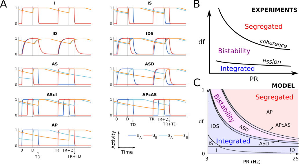
Figure 12: A. Time histories of all $2T\!R$-periodic states for $D\!<\!T\!D$ and $T\!D\!+\!D\!<\!T\!R$. B. Schematic diagram of the experimentally measured perceptual regions when varying $P\!R$ and $df$. C. Existence regions of the states in A. at varying $P\!R$ and $df$. States corresponding to integration, segregation or bistability are grouped by background colours (see Remark 8.2). Model parameters in C are: $\tau_{i}\!=\!0.2$, $\theta\!=\!0.5$, $T\!D\!=\!0.03$, $D\!=\!0.01$, $c\!=\!5$, $a\!=\!1$, $b\!=\!2$ and $m\!=\!6$.

Remark 8.1 (Extension to the case $T\!D\!+\!D\!\geq\!T\!R$).

The condition $T\!D\!+\!D\!<\!T\!R$ enabled us to obtain a complete classification of network states via the application of Lemma 2. However these states can exist also if $T\!D\!+\!D\!\geq\!T\!R$ with few adjustments in their existence conditions (see Supplementary Material LABEL:appendix_TD_D_gr_TR). We note that under this condition other $2T\!R$-periodic states exist, such as states where both units turn ON and OFF multiple times during each active tone interval (not shown). Since the condition $T\!D\!+\!D\!\geq\!T\!R$ is met for high values of $P\!R$ for which $T\!R\sim T\!D$, we explored this condition using computational tools (see Section 9).

8.1 Model states and link with auditory streaming

We now show how states described in the previous section can explain the emergence of different percepts during auditory streaming. In the following framework each possible percepts is linked ($\leftrightarrow$) with the units’ activities in the corresponding state:

• Integration $\leftrightarrow$ both units respond to all tones ($I$, $ID$, $IS$, $IDS$ and $AScI$).

• Segregation $\leftrightarrow$ no unit respond to both tones ($AP$).

• Bistability $\leftrightarrow$ one unit respond to both tones the other to only one tone ($AS$, $ASD$ and $APcAS$). This interpretation is motivated further in Remark 8.2.

Thus all model states presented in the previous section belong to one perceptual class. The cartoon in Figure 12B shows the experimentally detected regions of parameters $d\!f$ and $P\!R$ where participants are more likely to perceive integration, segregation or bistability (van Noorden diagram - see Introduction). We now validate our proposed framework of rhythm tracking by comparing model states consistent with different perceptual interpretations (percepts) in the $(d\!f,P\!R)$-plane. In these tests the model parameter $d$ is scaled by $df$ according to the monotonically decreasing function $d\!=\!c\cdot(1\!-\!df^{1/m})$, where $m$ is a positive integer and $df$ is a unitless parameter in $[0,1]$ (motivated in Section 3). Figure 12C shows regions of existence of model states when fixing all other parameters (as reported in the caption). States classified as integration, segregation and bistability are grouped by blue, red and purple background colors to facilitate the comparison with Figure 12B. The existence regions of states corresponding to integration and segregation qualitatively matches the perceptual organization in the van Noorden diagram.

Computation of the fission and coherence boundaries. Our analytical approach enables us to formulate the coherence and fission boundaries as functions of $P\!R$ using the states’ existence conditions. More precisely, the coherence boundary is the curve $d\!f_{coh}(P\!R)$ separating states $APcAS$ and $AP$, while the fission boundary is the curve $d\!f_{fiss}(P\!R)$ separating states $AScI$ and $IDS$:

$$\begin{gathered}d\!f_{coh}(P\!R)=[(a-bN^{+}+c-\theta)/c]^{m},\\ d\!f_{fiss}(P\!R)=[(a-bM^{+}+c-\theta)/c]^{m},\end{gathered}$$ (25)

where $N^{+}\!=\!e^{-(T\!R-D)/\tau_{i}}$ and $M^{+}\!=\!e^{-(2T\!R-T\!D)/\tau_{i}}$. The existence boundaries in Figure 12C (including these curves) naturally emerge from the model’s properties and are robust to parameter perturbations. For example, parameters $a$ and $b$ can respectively shift and stretch the two curves $d\!f_{coh}(P\!R)$ and $d\!f_{fiss}(P\!R)$. For all parameter combinations these curves have an exponential decay in $T\!R$ that generates regions of existence similar to the van Noorden diagram.

Remark 8.2.

The model predicts the emergence of integration, segregation and bistability in plausible regions of the parameter space. Yet, it currently cannot explain (1) how perception can switch between these two interpretations for fixed $d\!f$ and $P\!R$ values (i.e. perceptual bistability) and (2) which of the two tone streams is followed during segregation (i.e. A-A- or -B-B). This could be resolved in a competition network model, such as the one proposed by [16]. The selection of which rhythm is being followed by listeners at a specific moment in time would be resolved by a mutually exclusive selection of either unit: the perception is either integration if a unit responding to both tones is selected or segregation if a unit responding to every other tone is selected (see Discussion).

Remark 8.3 (A note on the word bistability).

Bistability (as used in Figure 12C) corresponds to states that encode both integrated and segregated rhythms simultaneously, where one unit responds to both tones and the other to one tone (say unit A responds ABAB…and unit B responds -B-B…). This should not be confounded with the fact that this bistable state coexists with another — by our definition — bistable state (unit A responds A-A-…and unit B responds ABAB…).

9 Computational analysis with smooth gain and inputs

In this section we extend the analytical results by running numerical simulations that use a continuous rather than Heaviside gain function and inputs, and reducing the timescale separation ratio $\tau_{i}/\tau$ by an order of magnitude. We restrict our study to $D\!<\!T\!D$ (the biologically realistic case), but without imposing the condition $T\!D\!+\!D\!<\!T\!R$. This allows us to make predictions at high $P\!R$s, which go beyond the analytic predictions of the previous section (see Remark 8.1). In summary, we find that this smooth, non-slow-fast regime generates similar states occupying slightly perturbed regions of stability. We consider a sigmoidal gain function $S(x)=[1+\exp(-\lambda x)]^{-1}$ with fixed slope $\lambda\!=\!30$, and we consider continuous inputs adapted from (3).

We classify integration (INT), segregation (SEG) and bistability (BIS) based on counting the number of threshold crossings during one periodic interval $[0,2T\!R]$. Let us call $n_{A}$ ($n_{B}$) the number of threshold crossings of unit A (B) and let $n\!=\!n_{A}\!+\!n_{B}$. Based on the correspondence between states and perception described in the previous section, states for which $n\!=\!4$ ($n\!=\!2$) correspond to integration (segregation) and states for which $n\!=\!3$ correspond to bistability. We run large parallel simulations to systematically study the convergence to the $2T\!R$-periodic states under changes in $d\!f$ and $P\!R$ and detect boundaries of transitions between different perceptual interpretations. We consider a grid of $l\times l$ uniformly spaced parameters $P\!R\in[1,40]$Hz and $d\!f\in[0,1]$ ($l\!=\!98$). For each node we run long simulations from the same initial conditions and compute the number of threshold crossings after the convergence to a stable $2T\!R$-periodic state for different values of $\tau$ (Figure 13A, B and C). There are 5 possible regions corresponding to one of four different values of $n\in\{0,2,3,4\}$. Three of these regions (as in panel A) correspond to the three colored regions found analytically in Figure 12C. Figure 13D shows example time histories of all the states in these five regions when $\tau\!=\!0.01$ (the values of $P\!R$ and $df$ are shown in white dots in panel B).

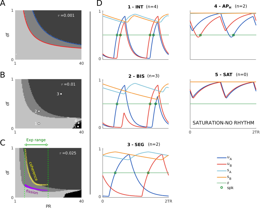
Figure 13: A-C. show the number of threshold crossings for both units $n$ in greyscale for simulated trajectories at varying $P\!R$ and $df$ (uniformly sampled in $96$ points) for different values of $\tau$ shown in top-right corner of each panel. Black corresponds to $n\!=\!0$ and the lightest gray to $n\!=\!4$. In A. the blue and red curves are the analytically predicted coherence and fission boundaries defined in equations 25. In C. yellow and purple crosses represent respectively the experimentally detected coherence and fission boundaries, replotted from Figure 2 in [46]. D. Time histories for the model states in each of the five regions of panel B, with values of $P\!R$ and $df$ shown by white dots in panel B. All parameters are as in Figure 3.

For low values of $\tau$ (panel A) the system is in the slow-fast regime. The blue and red curves show the analytically predicted coherence and fission boundaries for the Heaviside case under slow-fast regime defined in equations 25. These curves closely match the numerically predicted boundaries separating these regimes in the smooth system. For panel B and C $\tau$ is increased. All the existing states found in panel A persist and occupy the largest region of the parameter space, but the predicted fission and coherence boundaries perturb. We note that the selected values of $D$ and $T\!D$ in these figures lead to the condition $T\!D\!+\!D\!\geq\!T\!R$ for $P\!Rs$ greater than approximately $27$Hz, where the following two new $2T\!R$-periodic states appear:

$AP_{H}$ - characterized by $n\!=\!2$. Both units oscillate at higher activity levels than the threshold $\sim\theta$. Since $n\!=\!2$ this state may correspond to segregation, but its perceptual relevance is difficult to assess, because it occurs in a small region of the parameter space and at high $P\!Rs$, which is outside the range tested in psychoacoustic experiments.

$SAT$ - characterized by $n\!=\!0$. The activity of each units is higher than the threshold $\theta$ in $[0,2T\!R]$ (saturation). This state exists at (a) low $dfs$ and (b) high $P\!Rs$, greater than $30$Hz. Property (a) guarantees that inputs are strong enough to turn ON both units, while property (b) guarantees that that successive active tone intervals occur rapidly compared to the decay of the units’ activities. If $\tau$ is high, although the units turn OFF between two successive tone intervals, their slow decays does not allow crossings of the threshold $\theta$. This state does not correspond to any percepts studied in the auditory streaming experiments (integration or segregation). However, $P\!R$ typically ranges between 5 and 20Hz in these experiments. The existence of this state may explain why perceivable isochronal rhythms above $\sim 30$ Hz are heard as a pure tone in the first (lowest) octave of human hearing. Indeed, when $df\!=\!0$ the model inputs represent the repetition of a single tone (B=A) with frequency $P\!R$. Our proposed framework linking percepts to neural states (see previous section) suggests that $SAT$ cannot track any rhythm simply because no unit crosses threshold.

The coherence and fission boundaries detected from the network simulations in panel Figure 13C quantitatively match those from psychoacoustic experiments (yellow and purple crosses, the available data spans $P\!Rs$ in $\sim[7,20]$Hz). The model parameters chosen in the this figure (including $\tau$) have been manually tuned to match the data. Overall, we conclude that the proposed modelling framework is a good candidate for explaining the perceptual organization in the van Noorden diagram and for perceiving repeated tones (isochronal rhythms) at high frequencies as single pure tone in the lowest octave of human hearing.

10 Discussion

We proposed a minimal firing rate model of ambiguous rhythm perception. Four delay differential equations represent two neural populations coupled by fast direct excitation and slow delayed inhibition that are forced by square-wave periodic inputs. Acting on different timescales, excitation and inhibition give rise to rich dynamics driven by cooperation and competition. We used analytical and computational tools to investigate periodic solutions 1:1 locked to the inputs (1:1 locked states) and their dependence on parameters influencing auditory perception.

The model incorporates neural mechanisms commonly found in auditory cortex (ACx). We hypothesised that pitch and rhythm are respectively encoded in tonotopic primary and secondary ACx [11]. Model units represent populations in secondary ACx - i.e. the belt or parabelt regions of auditory cortex - receiving inputs that mimic primary ACx responses [48] to interleaved A and B tones [13]. This division of roles in ACx is supported by evidence for specific non-primary belt and parabelt regions encoding temporal features (i.e. rhythmicity) only present in sound envelope rather stimulus features (i.e. content like pitch) as in primary ACx [11]. Model inputs depend on key parameters influencing psychoacoustic perception: the presentation rate ($P\!R$), the tones’ pitch difference ($df$) and the tone duration ($T\!D$). The timescale separation between excitation and inhibition is consistent with AMPA and GABA synapses, respectively (widely found in cortex). The inhibition - with delay assumed fixed to $D$ - could be affected by factors including slower inhibitory activation times (vs excitatory), indirect connections and propagation times between the spatially separated A and B populations.

By posing the model in a slow-fast regime we studied 1:1 locked states for $T\!D\!+\!D\!<\!1/P\!R$, which enabled us to classify states and define a matrix representation (matrix form). This mathematical tool helped us to formulate existence conditions and rule out impossible states, leading to a complete description of all 1:1 locked states. The condition $T\!D\!+\!D\!<\!1/P\!R$ is relevant to auditory streaming. Indeed, the factors that may play a role in generating delayed inhibition discussed above would most likely lead to short or moderate delays, for which this condition is guaranteed for the value of $P\!R$s and $T\!D$s typically considered in experiments ($P\!R\in[5,20]$Hz and $T\!D\in[10,30]$ms; $T\!D$’s interpretation discussed below in Predictions).

We proposed a classification of 1:1 locked states and for rhythms heard during auditory streaming based on threshold crossing of the units’ responses. More precisely, for ABAB integrated percepts both units respond to every tone and for segregated A-A- or -B-B percepts each unit responds to only one tone. Bistability corresponds to one unit responding to every tone and the other unit responding to every other tone. This interpretation of bistability can explain how both integrated and segregated rhythms may be perceived simultaneously, as reported in some behavioral studies [49, 50], but not the dynamic alternation between these two percepts [51, 16] (see the section “Future work” below). This classification enabled us to compare the states’ existence regions to those of the corresponding percepts when varying $df$ and $P\!R$ in experiments (van Noorden diagram). A similar organization of these regions emerged naturally from the model and is robust to parameter perturbations.

Finally, we carried out numerical analysis with a smooth gain function, smooth inputs and different levels of timescale separation to confirm the validity of the analytical approach. The simulations closely matched the analytical predictions under the slow-fast regime. Reducing the timescale separation shifts the regions of existence of the perceptually relevant states and produces a qualitatively close match the van Noorden diagram. Numerical simulations extended this analysis to $T\!D\!+\!D\!\geq\!1/P\!R$, which led to the emergence of a high activity (saturated) state occurring at high $P\!R$s and low $df$. The case $T\!D\!+\!D\!\geq\!1/P\!R$ may lead to the existence other states not analyzed as they do not appear in the van Noorden $(P\!R,df)$-range.

10.1 Models of neural competition

Our proposed model addresses the formation of percepts but not switching between them, so-called auditory perceptual bistability [51, 16]. Future work will consider the present description acts as a front-end to a competition network (one can think of the present study as a reformulation of the pre-competition stages in [16]). Perceptual bistability (e.g. binocular rivalry) is the focus of many theoretical studies that feature mechanisms and dynamical states similar to those reported here. We note a key distinction here: the units are associated with tonotopic locations of the A and B tones, not with percepts as in many other models. In contrast with our study, firing rate models are widely used with fixed inputs, mutual inhibition (often assumed instantaneous), and a slow adaptation process that drives slow-fast oscillations [21, 22, 23]. Periodic inputs associated with specific experimental paradigms have been considered in several models [27, 42, 28, 52, 53].

10.2 Models of auditory streaming

The auditory streaming paradigm has been the focus of a wealth of electrophysiological and imaging studies in recent decades. However, it has received far less attention from modelers when compared with visual paradigms. Many existing models of auditory streaming have used signal-processing frameworks without a link to neural computations (recent reviews: [14, 15, 12]). In contrast our model is based on a plausible network architecture with biophysically constrained and meaningful parameters. Simplifications (like the Heaviside gain function) provide the tractability to perform a detailed analysis of all states relevant to perceptual interpretations and find their existence conditions. Despite the model’s apparent simplicity (4 DDEs) it produces a rich repertoire of dynamical states linked to perceptual interpretations. Our model is a departure from (purely) feature-based models because it incorporates a combination of mechanisms acting at timescales close to the interval between tones. By contrast, [46] considers neural dynamics only on a fast time scale (less than TR). Further, [16] considers slow adaptation ($\tau>1$ s) to drive perceptual alternations, assumes instantaneous inhibition and slow NMDA-excitation, a combination that precludes forward masking as reported in [13]. The entrainment of intrinsic oscillations to inputs was considered in [17], albeit using a highly redundant spatio-temporal array of oscillators. Recently, a parsimonious neural oscillator framework was considered in [18] but without addressing how the same percepts persist over a wide range of $P\!R$ (5-20 Hz).

A central hypothesis for our model is that network states associated with different perceptual interpretations are generated before entering into competition that produces perceptual bistability (as put forward in [54] with a purely algorithmic implementation). Here network states are emergent from a combination of neural mechanisms: mutual fast, direct excitation and mutual slow acting, delayed inhibition. In contrast with [16] our model is sensitive to the temporal structure of the stimulus present in our stereotypical description of inputs to the model from primary auditory cortex and over the full range of stimulus presentation rates.

10.3 Predictions

In van Noorden’s original work on auditory streaming boundaries in the $(df,P\!R)$-plane were identified: the temporal coherence boundary below which only integrated occurs and the fission boundary above which only segregated occurs. We derived exact expressions for these behavioral boundaries that match the van Noorden diagram. One of challenges in developing a model that reproduces the van Noorden diagram was to explain how a neural network can produce an integrated-like state at very large $df$-values and low $P\!R$s. Primary ACx shows no tonotopic overlap in this parameter range (A-location neurons exclusively respond to A tones) [13]. Our results show that fast excitation can make this possible. Disrupting AMPA excitation is predicted to preclude the integrated state at large $df$-values. Furthermore, our results show that segregation relies on slow acting, delayed inhibition, which performs forward masking. Whilst the locus for this GABA-like inhibition cannot yet be specified, we predict that its disruption would promote the integrated percept.

Some model parameters (i.e. $T\!D$, $T\!R$, input strengths) can readily be tested in experiments by changing sound inputs. The model could predict the effect of such changes on perception. However, the role of $T\!D$ has yet to be investigated in experiments. In our model $T\!D$ better represents the duration of the primary ACx responses to tones, rather than the sound duration of each tone. This interpretation is supported by recordings of firing rates at tonotopic locations in Macaque primary ACx [13]. In these data $\sim 80\%$ of the response is localized shortly after the tone onset. This time window is approximately constant $\sim 30$ms across different tone intervals, tone durations, $P\!R$ and $d\!f$ (unpublished results).

Numerics for the smooth model predict a region at large $P\!R$s for which responses are saturated (no threshold crossings). These responses are consistent with rapidly repeating discrete sound events at rates above $30$Hz sounding like a low-frequency tone ($20$Hz is typically quoted as the lowest frequency for human hearing). At presentation rates above $30$Hz we predict a transition from hearing a modulated low-frequency tone to hearing two fast segregated streams as df is increased.

10.4 Conclusion

Our study proposed that sequences of tones are perceived as integrated or segregated through a combination of feature-based and temporal mechanisms. Here tone frequency is incorporated via input-strengths and timing mechanisms are introduced via excitatory and inhibitory interactions at different timescales including delays. We suspect that the proposed architecture is not unique in being able to produce similar dynamic states and the van Noorden diagram. The implementation of globally excitatory inputs ($i_{A}(t)$ and $i_{B}(t)$ driving both units) rather than mutual fast-excitation is expected to produce similar results.

The resolution of competition between these states is not considered at present. Imaging studies implicate a network of brain areas (e.g. frontal and parietal) extending beyond auditory cortex for streaming [55, 56, 57, 58], some of which are generally implicated in perceptual bistability [59, 60, 61]. The model could be extended to consider perceptual competition and bistability by incorporating a competition stage further downstream (in the same spirit as [16]). An extended framework would provide the ideal setting to explore perceptual entrainment through the periodic [62] or stochastic [63] modulation of a parameter like $df$.

Funding

This work was funded by the EPSRC funding project Reference EP/R03124X/1.

Abbreviations

ACx - auditory Cortex; $T\!D$ - tone duration; $T\!R$ - tone repetition time; $P\!R$ - presentation rate.

Availability of data and materials

Source code to reproduce the results presented will be made available on a public GitHub repository at the time of publication.

Ethics approval and consent to participate

Not applicable.

Competing interests

The authors declare that they have no competing interests.

Consent for publication

Not applicable.

Authors’ contributions

AF and JR were involved with the problem formulation, model design, discussion of results and writing the manuscript. AF carried out the mathematical analysis and numerical simulations.

11 Supplementary Material

11.1 Separatrices

In this section we derive that separatrices of the degenerate fixed point $(s_{1},s_{2})$ of system

$$\begin{array}[]{lcl}u_{A}^{\prime}&=&-u_{A}+H(a(u_{B}-s_{2}))\\ u_{B}^{\prime}&=&-u_{B}+H(a(u_{A}-s_{1}))\end{array}$$ (26)

are given by

$$\begin{cases}(u_{A}-1)s_{2}/(s_{1}-1)&\mbox{if }u_{A}\leq s_{1}\\ u_{A}(s_{2}-1)/s_{1}+1&\mbox{otherwise}\end{cases}$$

We prove that these curves define the separatrices by showing the convergence of orbits from initial conditions $(u_{A}^{0},u_{B}^{0})$ in the top left corner in Figure 4 to $(1,1)$ (purple trajectories in Figure 4). A similar proof holds for initial conditions in other regions of the phase-space and for convergence to $(0,0)$. Points $(u_{A}^{0},u_{B}^{0})$ in the top left corner belong to the set: Ω_L = { (u_A,u_B) : u_A ¡ s_1 and u

References

- [1] Cherry EC. Some experiments on the recognition of speech, with one and with two ears. The Journal of the acoustical society of America. 1953;25(5):975–979.
- [2] Bizley JK, Cohen YE. The what, where and how of auditory-object perception. Nat Rev Neurosci. 2013;14(10):693–707.
- [3] Hubel DH, Wiesel TN. Receptive fields, binocular interaction and functional architecture in the cat’s visual cortex. The Journal of physiology. 1962;160(1):106–154.
- [4] Ben-Yishai R, Bar-Or RL, Sompolinsky H. Theory of orientation tuning in visual cortex. Proc Natl Acad Sci USA. 1995;92(9):3844.
- [5] Bressloff PC, Cowan JD, Golubitsky M, Thomas PJ, Wiener MC. Geometric visual hallucinations, Euclidean symmetry and the functional architecture of striate cortex. Philos Trans R Soc Lond B Biol Sci. 2001;356(1407):299–330.
- [6] Rankin J, Chavane F. Neural field model to reconcile structure with function in primary visual cortex. PLoS computational biology. 2017;13(10):e1005821.
- [7] Romani GL, Williamson SJ, Kaufman L. Tonotopic organization of the human auditory cortex. Science. 1982;216(4552):1339–1340.
- [8] Da Costa S, van der Zwaag W, Marques JP, Frackowiak RS, Clarke S, Saenz M. Human primary auditory cortex follows the shape of Heschl’s gyrus. The Journal of Neuroscience. 2011;31(40):14067–14075.
- [9] van Noorden L. Temporal coherence in the perception of tone sequences. PhD Thesis, Eindhoven University; 1975.
- [10] Pressnitzer D, Sayles M, Micheyl C, Winter I. Perceptual organization of sound begins in the auditory periphery. Curr Biol. 2008;18(15):1124–1128.
- [11] Musacchia G, Large EW, Schroeder CE. Thalamocortical mechanisms for integrating musical tone and rhythm. Hearing research. 2014;308:50–59.
- [12] Rankin J, Rinzel J. Computational models of auditory perception from feature extraction to stream segregation and behavior. Curr Opin Neurobiol. 2019;58:46–53.
- [13] Fishman YI, Arezzo JC, Steinschneider M. Auditory stream segregation in monkey auditory cortex: effects of frequency separation, presentation rate, and tone duration. J Acoust Soc Am. 2004;116(3):1656–1670.
- [14] Snyder JS, Elhilali M. Recent advances in exploring the neural underpinnings of auditory scene perception. Ann NY Acad Sci. 2017;.
- [15] Szabó BT, Denham SL, Winkler I. Computational Models of Auditory Scene Analysis: A Review. Front Neurosci. 2016;10.
- [16] Rankin J, Sussman E, Rinzel J. Neuromechanistic model of auditory bistability. PLoS computational biology. 2015;11(11).
- [17] Wang D, Chang P. An oscillatory correlation model of auditory streaming. Cogn Neurodynamics. 2008;2(1):7–19.
- [18] Pérez-Cervera A, Ashwin P, Huguet G, M-Seara T, Rankin J. The uncoupling limit of identical Hopf bifurcations with an application to perceptual bistability. J Math Neuro. 2019;9(1):7.
- [19] Moore BC. An introduction to the psychology of hearing. Brill; 2012.
- [20] Wilson HR, Cowan JD. Excitatory and Inhibitory Interactions in Localized Populations of Model Neurons. Biophys J. 1972;12(1):1–24.
- [21] Laing CR, Chow CC. A spiking neuron model for binocular rivalry. Journal of computational neuroscience. 2002;12(1):39–53.
- [22] Shpiro A, Curtu R, Rinzel J, Rubin N. Dynamical Characteristics Common to Neuronal Competition Models. J Neurophysiol. 2007;97(1):462–473.
- [23] Curtu R, Shpiro A, Rubin N, Rinzel J. Mechanisms for frequency control in neuronal competition models. SIAM J Appl Dyn Syst. 2008;7(2):609–649.
- [24] Diekman C, Golubitsky M, McMillen T, Wang Y. Reduction and dynamics of a generalized rivalry network with two learned patterns. SIAM J Appl Dyn Syst. 2012;11(4):1270–1309.
- [25] Diekman CO, Golubitsky M. Network symmetry and binocular rivalry experiments. The Journal of Mathematical Neuroscience (JMN). 2014;4(1):1–29.
- [26] Wang XJ. Probabilistic decision making by slow reverberation in cortical circuits. Neuron. 2002;36(5):955–968.
- [27] Wilson HR. Computational evidence for a rivalry hierarchy in vision. Proc Natl Acad Sci USA. 2003;100(24):14499–14503.
- [28] Vattikuti S, Thangaraj P, Xie HW, Gotts SJ, Martin A, Chow CC. Canonical cortical circuit model explains rivalry, intermittent rivalry, and rivalry memory. PLoS Comput Biol. 2016;12(5):e1004903.
- [29] Farcot E, Gouzé JL. Limit cycles in piecewise-affine gene network models with multiple interaction loops. International Journal of Control. 2010;41(1):119–130.
- [30] Rinzel J, Ermentrout GB. Analysis of neural excitability and oscillations. Methods in neuronal modeling. 1998;2:251–292.
- [31] Izhikevich EM. Dynamical systems in neuroscience. MIT press; 2007.
- [32] Ermentrout GB, Terman DH. Mathematical foundations of neuroscience. vol. 35. Springer Science & Business Media; 2010.
- [33] Desroches M, Guillamon A, Ponce E, Prohens R, Rodrigues S, Teruel AE. Canards, folded nodes, and mixed-mode oscillations in piecewise-linear slow-fast systems. SIAM review. 2016;58(4):653–691.
- [34] Curtu R. Singular Hopf bifurcations and mixed-mode oscillations in a two-cell inhibitory neural network. Physica D. 2010;239(9):504–514.
- [35] Marder E, Calabrese RL. Principles of rhythmic motor pattern generation. Physiological reviews. 1996;76(3):687–717.
- [36] Rubin J, Terman D. Geometric analysis of population rhythms in synaptically coupled neuronal networks. Neural computation. 2000;12(3):597–645.
- [37] Wang XJ, Rinzel J. Alternating and synchronous rhythms in reciprocally inhibitory model neurons. Neural computation. 1992;4(1):84–97.
- [38] Ferrario A, Merrison-Hort R, Soffe SR, Li W, Borisyuk R. Bifurcations of limit cycles in a reduced model of the Xenopus tadpole central pattern generator. J Math Neuro. 2018;8(1):10.
- [39] Ashwin P, Coombes S, Nicks R. Mathematical frameworks for oscillatory network dynamics in neuroscience. J Math Neuro. 2016;6(1):2.
- [40] Campbell SA. Time delays in neural systems. In: Handbook of brain connectivity. Springer; 2007. p. 65–90.
- [41] Dhamala M, Jirsa VK, Ding M. Enhancement of neural synchrony by time delay. Physical review letters. 2004;92(7):074104.
- [42] Jayasuriya S, Kilpatrick ZP. Effects of time-dependent stimuli in a competitive neural network model of perceptual rivalry. B Math Biol. 2012;74(6):1396–1426.
- [43] Bressloff PC. Spatiotemporal dynamics of continuum neural fields. Journal of Physics A: Mathematical and Theoretical. 2011;45(3):033001.
- [44] Micheyl C, Tian B, Carlyon R, Rauschecker J. Perceptual organization of tone sequences in the auditory cortex of awake macaques. Neuron. 2005;48(1):139–148.
- [45] Scholes C, Palmer AR, Sumner CJ. Stream segregation in the anesthetized auditory cortex. Hearing research. 2015;328:48–58.
- [46] Almonte F, Jirsa V, Large E, Tuller B. Integration and segregation in auditory streaming. Physica D. 2005;212(1):137–159.
- [47] Rohatgi A. WebPlotDigitizer. Austin, Texas, USA; 2017. Last accessed on 23/06/2020.
- [48] Hackett TA, de la Mothe LA, Camalier CR, Falchier A, Lakatos P, Kajikawa Y, et al. Feedforward and feedback projections of caudal belt and parabelt areas of auditory cortex: refining the hierarchical model. Frontiers in neuroscience. 2014;8:72.
- [49] Denham SL, Bendixen A, Mill R, Tóth D, Wennekers T, Coath M, et al. Characterising switching behaviour in perceptual multi-stability. J Neurosci Methods. 2012;210(1):79–92.
- [50] Denham SL, Bohm T, Bendixen A, Szalárdy O, Kocsis Z, Mill R, et al. Stable individual characteristics in the perception of multiple embedded patterns in multistable auditory stimuli. Front Neurosci. 2014;8(25):1–15.
- [51] Pressnitzer D, Hupé J. Temporal dynamics of auditory and visual bistability reveal common principles of perceptual organization. Curr Biol. 2006;16(13):1351–1357.
- [52] Li HH, Rankin J, Rinzel J, Carrasco M, Heeger D. Attention model of binocular rivalry. P Natl Acad Sci Usa. 2017;114(30):E6192–E6201.
- [53] Darki F, Rankin J. Methods to assess binocular rivalry with periodic stimuli. J Math Neuro. 2020;10.
- [54] Mill R, Bőhm T, Bendixen A, Winkler I, Denham S. Modelling the emergence and dynamics of perceptual organisation in auditory streaming. PLoS Comput Biol. 2013;9(3):e1002925.
- [55] Cusack R. The intraparietal sulcus and perceptual organization. J Cognit Neurosci. 2005;17(4):641–651.
- [56] Kanai R, Bahrami B, Rees G. Human parietal cortex structure predicts individual differences in perceptual rivalry. Curr Biol. 2010;20(18):1626–1630.
- [57] Kashino M, Kondo H. Functional brain networks underlying perceptual switching: auditory streaming and verbal transformations. Philos T Roy Soc B. 2012;367(1591):977–987.
- [58] Kondo HM, Pressnitzer D, Shimada Y, Kochiyama T, Kashino M. Inhibition-excitation balance in the parietal cortex modulates volitional control for auditory and visual multistability. Scientific reports. 2018;8(1):14548.
- [59] Vernet M, Brem AK, Farzan F, Pascual-Leone A. Synchronous and opposite roles of the parietal and prefrontal cortices in bistable perception: A double-coil TMS–EEG study. Cortex. 2015;64:78–88.
- [60] Wang M, Arteaga D, He BJ. Brain mechanisms for simple perception and bistable perception. Proc Natl Acad Sci USA. 2013;110(35):E3350–E3359.
- [61] Zaretskaya N, Thielscher A, Logothetis NK, Bartels A. Disrupting parietal function prolongs dominance durations in binocular rivalry. Curr Biol. 2010;20(23):2106–2111.
- [62] Byrne Á, Rinzel J, Rankin J. Auditory streaming and bistability paradigm extended to a dynamic environment. Hearing Res. 2019;383:107807.
- [63] Baker DH, Richard B. Dynamic properties of internal noise probed by modulating binocular rivalry. PLoS Comput Biol. 2019 06;15(6):1–18.