Bayesian Analysis of the ⁷⁰Zn$(d,^{3}\textnormal{He})^{69}$Cu Transfer Reaction

Abstract

Transfer reactions provide information about the single-particle nature of nuclear levels. In particular, the differential cross sections from these measurements are sensitive to the angular momentum of the transferred particle and the spectroscopic factor of the populated level. However, the process of extracting these properties is subject to uncertainties, both from experimental and theoretical sources. By integrating the distorted wave Born approximation into a Bayesian model, we propagate these uncertainties through to the spectroscopic factors and orbital angular momentum values. We use previously reported data of the proton pickup reaction ⁷⁰Zn$(d,^{3}\textnormal{He})^{69}$Cu as an example. By accounting for uncertainties in the experimental data, optical model parameters, and reaction mechanism, we find that the extracted spectroscopic factors for low lying states of ⁶⁹Cu are subject to large, asymmetric uncertainties ranging from $35\%$ to $108\%$. Additionally, Bayesian model comparison is employed to assign probabilities to each of the allowed angular momentum transfers. This method confirms the assignments for many states, but suggests that the data for a state lying at $3.70$ MeV is better characterized by an $\ell=3$ transfer, rather than the previously reported $\ell=2$.

I Introduction

Nucleon transfer reactions are critical tools for studying the single particle structure in nuclei. However, their usefulness depends upon a successful theoretical description of the reaction mechanism. By far the most widely used methodology is the combination of the nuclear optical model Feshbach (1958) and the Distorted Wave Born Approximation (DWBA) (see Ref. Macfarlane and French (1960) and references therein). By using DWBA it becomes possible to determine both the transferred angular momentum, $\ell$, and spectroscopic factor of the populated single particle or hole state Satchler (1983). This structure information can in turn be used to answer questions in nuclear astrophysics Bardayan (2016), and to test the shell model on isotopes located far from stability Wimmer (2018).

Despite the wide use of these methods, quantifying the uncertainties associated with both the optical potentials and the reaction model has been a long standing issue. Previous studies have used statistical methods to determine the uncertainty on the potential parameters Varner et al. (1991), but little work has been done to propagate these uncertainties through DWBA calculations in a statistically meaningful way. To data, most spectroscopic factors are reported with either no uncertainty, an assumed equivalence between the uncertainty in the data normalization and that of the spectroscopic factor, or a constant $25\%$ determined from historical studies Endt (1977).

Over the last few years, these issues have led to a renewed focus on the impact of optical model parameters on transfer reactions. A series of studies has focused on the nature and magnitude of this effect Lovell and Nunes (2015); Lovell et al. (2017); King et al. (2018). The first steps have also been taken towards quantifying these uncertainties using Bayesian statistics Lovell and Nunes (2018); King et al. (2019). These studies focus on the broad effects of optical potentials, but it is worthwhile to establish a Bayesian framework in which the results of a single experiment can be analyzed. The goal of this paper is to establish such a framework and to examine the possible implications on future experiments.

The methods developed and presented here will be applied to the analysis of the proton pickup reaction ${}^{70}\textnormal{Zn}(d,^{3}\textnormal{He})^{69}\textnormal{Cu}$, which was originally reported in Ref. Morfouace et al. (2016). This data set possesses many of the features typical of a transfer measurement study: the use of a high resolution magnetic spectrograph to resolve the excited states of interest, elastic data for the entrance channel collected with the same target and beam, experimental uncertainties coming from counting statistics, and limited angular coverage in both the elastic scattering and transfer differential cross sections. The previous analysis assigned $\ell$ values and extracted spectroscopic factors for the first eight excited states of ${}^{69}\textnormal{Cu}$. Our reanalysis aims to determine the uncertainties associated with these quantities using Bayesian statistics.

This paper will be structured to introduce the relevant reaction theory in Sec. II, explain and construct the Bayesian model in Sec. III, and finally present and then discuss the results in Sec. IV and Sec. V, respectively.

II Reaction Theory

II.1 The Optical Model

The nuclear optical model simplifies the multi-nucleon scattering problem by considering a single particle interacting with a complex potential, $\mathcal{U}(r)$. The theoretical basis for this procedure was first established in Ref. Feshbach (1958), but fell short of actually prescribing the form of the complex potential. Through detailed analysis of elastic scattering from a range of targets and energies, Ref. Becchetti and Greenlees (1969a) developed a phenomenological form for the optical model. Our work will be focused on the effect of these phenomenological potential parameters, but further theoretical and historical details can be found in Ref. Hodgson (1971). For our work we adopt the following form of the optical potential:

$$\mathcal{U}(r)=V_{c}(r;r_{c})-Vf(r;r_{0},a_{0})\\ -i(W-4a_{i}W_{s}\frac{d}{dr_{i}})f(r;r_{i},a_{i})\\ +(\frac{\hbar}{m_{\pi}c})^{2}V_{so}\frac{1}{r}\frac{d}{dr}f(r;r_{so},a_{so})\bm{\sigma}\cdot\bm{\ell},$$ (1)

where $f(r)$ is given by the Wood-Saxon form factor:

$$f(r;r_{0},a_{0})=\frac{1}{1+\exp(\frac{r-r_{0}A_{t}^{1/3}}{a_{0}})}.$$ (2)

Each term in $\mathcal{U}$ is parameterized with a well depth, ${V,W,W_{s}}$, radius, ${r_{0},r_{i},r_{so}}$, and diffuseness, ${a_{0},a_{i},a_{so}}$. $A_{t}$ is the mass number of the target nucleus. Additionally, the spin orbit term has an interaction based on the projectile orbital and spin angular momentum, $\bm{\ell}$ and $\bf{s}$, respectively. In this case $\bm{\sigma}=2\bf{s}$, and $(\frac{\hbar}{m_{\pi}c})^{2}$ is a constant with a value of approximately $2$ fm². The Coulomb term, $V_{c}$, comes from the potential of a uniformly charged sphere with radius $R_{c}=r_{c}A_{t}^{1/3}$. These conventions are adopted in order to be consistent with the code FRESCO Thompson , and care should be taken to convert values given in this paper if a different set of conventions is adopted.

The phenomenological optical model uses experimental data, typically differential elastic scattering cross sections and analyzing powers, to determine the parameter values defined above. Local fits of these parameters, like those listed in Ref. Perey and Perey (1976), try to best reproduce the results of elastic scattering from a single target nucleus at a single energy. Global fits, such as Refs. Varner et al. (1991); Becchetti and Greenlees (1969a, b); Beccehetti and Greenless (1969); Pang et al. (2009); Daehnick et al. (1980), use a variety of targets and beam energies to derive relations between potential parameters and target mass, beam energy, and other nuclear properties.

II.2 Distorted Wave Born Approximation

The shape and magnitude of transfer reaction differential cross sections are directly related to the angular momentum of the transferred nucleon and the spectroscopic factor of the populated nuclear state. Thus, a theoretical description of the cross section will allow the extraction of these properties from experimental data. DWBA is a perturbative method that uses the optical potentials of Sec.II.1 to model the entrance and exit channels, and a transition operator for the transferred particle or cluster. Expressing this transition operator explicitly for the $A(d,^{3}\!\textnormal{He})B$ pickup reaction, we can write it in either the prior or post form:

$$\mathcal{V}_{\textnormal{prior}}=V_{p+d}+\mathcal{U}_{d+B}-\mathcal{U}_{d+A}$$ (3)

$$\mathcal{V}_{\textnormal{post}}=V_{p+B}+\mathcal{U}_{d+B}-\mathcal{U}_{{}^{3}\textnormal{He}+B}.$$ (4)

$\mathcal{U}$ are the optical potentials for each of the reaction channels. The entrance, exit, and core-core systems are denoted by $A+d$, $B+^{3}\textnormal{He}$, and $B+d$, respectively. The $V$ potentials are the binding potentials for the proton on either the projectile or target nucleus. The first order $T$ matrix for the transfer from channel $\alpha$ to channel $\beta$ in the prior form is given by:

$$T_{\beta\alpha}=J\int d\bm{r}_{{}^{3}\textnormal{He}}\int d\bm{r}_{d}\\ \chi_{\beta}^{(-)*}(\bm{r}_{{}^{3}\textnormal{He}},\bm{k}_{{}^{3}\textnormal{He}})\bra{B,^{3}\textnormal{He}}\mathcal{V}_{\textnormal{prior}}\ket{A,d}\chi_{\alpha}^{(+)}(\bm{r}_{d},\bm{k}_{d}),$$ (5)

where $\chi$ is the distorted wave generated from the corresponding optical potential, J is the Jacobian for the transformation to the two coordinates, and the kets refer to the internal coordinates of the respective nuclei. Further information on the derivation of these equations and other theoretical considerations can be found in Refs. Satchler (1983); Thompson and Nunes (2009).

II.3 Cross Section Calculations

All transfer and elastic differential cross sections for this work were calculated using the coupled-channels reaction code FRESCO Thompson . The FRESCO transfer differential cross section can be related to experiment through:

$$\frac{d\sigma}{d\Omega}_{exp}=C^{2}S_{\textnormal{p}}C^{2}S_{\textnormal{t}}\frac{d\sigma}{d\Omega}_{FRESCO}.$$ (6)

The two spectroscopic factors and isospin Clebsch-Gordan coefficients are for the projectile and target system, respectively. For particles with $A\leq 4$, the spectroscopic factor can be approximated by $\frac{A}{2}$ Satchler (1983). Thus, for the $d+p$ system, $C^{2}S_{\textnormal{p}}=\frac{3}{2}$. Since $C^{2}S_{\textnormal{p}}$ is assumed constant, any further reference to $C^{2}S$ will be equivalent to $C^{2}S_{\textnormal{t}}$.

In order to reduce the computational cost of the transfer calculations, this work uses the zero-range approximation Satchler (1983). This approximation, in the specific case of the pick-up reaction $A(d,^{3}\!\textnormal{He})B$, takes the prior form of Eq. (3) and sets $\mathcal{U}_{d+B}-\mathcal{U}_{d+A}$ to zero, a procedure justified by experimental observation Lee et al. (1964). The projectile is then assumed to be absorbed and emitted from the same point giving:

$$\bra{d}V_{pd}\ket{{}^{3}\textnormal{He}}\sim D_{o}\delta(\mathbf{r_{p}}),$$ (7)

where $\ket{{}^{3}\textnormal{He}}$, $\ket{d}$ are the internal wave functions of the ejectile and projectile, respectively, $D_{0}$ is the volume integral of the interaction strength, $V_{pd}$ is the binding potential of the proton to the deuteron, and $\mathbf{r_{p}}$ is the coordinate of the proton relative to the deuteron. Use of this approximation gives us the further benefit of a direct comparison to the original analysis of ⁷⁰Zn$(d,^{3}\textnormal{He})^{69}$Cu that used the zero-range code DWUCK4 for the extraction of $C^{2}S_{t}$ Kunz . It should be noted that Ref.Morfouace et al. (2016) also performed finite-range calculations, but the computational costs are prohibitively expensive in the present analysis. The value of $D_{0}$ is calculated theoretically, with the historical value for proton pick-up and stripping reactions being $D_{0}=-172.8$ MeV fm^3/2 Bassel (1966). Comparing the different models in Ref. Goldfarb et al. (1973), an approximately $15\%$ spread in the values of $D_{0}^{2}$ is observed. This is inline with the findings of Ref. Bertone et al. (2002), which also noted an approximate $15\%$ spread in the product $(C^{2}S_{\textnormal{p}})D_{0}^{2}$. We adopt the above value with its associated uncertainty; however, Ab initio methods, such as those in Ref. Brida et al. (2011), now offer more precise determinations of the $\braket{d}{{}^{3}\textnormal{He}}$ overlap. If $D_{0}$ is deduced using these methods, then this additional source of uncertainty will be effectively eliminated. As a direct consequence the uncertainty in $C^{2}S_{\textnormal{t}}$ will be reduced by about $15\%$.

III Bayesian Inference

As discussed in Sec. II.1, the potential parameters of the phenomenological optical model are constrained by fitting to experimental data. Thus, their values are inherently subject to uncertainty, which will ultimately propagate through to any quantity extracted using them. Bayesian inference treats this interaction between measured data and model parameters as a logical relationship between conditional probabilities S Sivia and Skilling (2006). This relationship is expressed in Bayes’ theorem:

$$P(\bm{\theta}|\mathbf{D})=\frac{P(\mathbf{D}|\bm{\theta})P(\bm{\theta})}{\int_{\bm{\theta}}P(\bm{D}|\bm{\theta})P(\bm{\theta})d\bm{\theta}},$$ (8)

where the posterior probability distribution, $P(\bm{\theta}|\mathbf{D})$, is the conditional probability of the model parameters, $\bm{\theta}$, given the data, $\mathbf{D}$. The posterior is calculated from the likelihood function, $P(\mathbf{D}|\bm{\theta})$, prior probabilities, $P(\bm{\theta})$, and the evidence integral, $\int_{\bm{\theta}}P(\bm{D}|\bm{\theta})P(\bm{\theta})d\bm{\theta}$. Prior probabilities represent our knowledge of the parameters before the data is considered, and must be assigned for every parameter that we want to estimate. The likelihood function must also be specified, and will express, in probabilistic terms, how the parameters of the model relate to the data. This function is also present in the frequentist approach, with a common example being the $\chi^{2}$ function. The evidence ensures that the product of the likelihood and the priors is normalized. For this work one of our main goals will be to estimate the posterior distribution for the spectroscopic factor. This will require that we assign priors for every optical model potential parameter and the spectroscopic factor itself. These prior probabilities will then be updated through the likelihood function using the experimentally measured cross sections for the elastic and transfer channels.

Bayes’ theorem is also central to our other goal of determining the most probable angular momentum transfer for a given state. This problem belongs to a subcategory of Bayesian inference called model selection. Computing the probability for a model, $M_{j}$, can be done by restating Bayes’ theorem:

$$P(M_{j}|\mathbf{D})=\frac{P(\mathbf{D}|M_{j})P(M_{j})}{\sum_{i}P(\mathbf{D}|M_{i})P(M_{i})}.$$ (9)

This expression is built on the same logical foundation as Eq. (8), but has been adapted to compute posterior distributions for $M_{j}$, which means a comparison can now be made between different models. For each $M_{j}$ there is a set of model parameters $\bm{\theta}_{j}$ which have been marginalized over. This means:

$$P(\mathbf{D}|M_{j})=\int P(\mathbf{D}|M_{j},\bm{\theta}_{j})P(\bm{\theta}_{j}|M_{j})d\bm{\theta}_{j}.$$ (10)

Based on this equation it can be seen that $P(\mathbf{D}|M_{j})$ is equivalent to the evidence integral from Eq. (8). Thus, in order for us to evaluate how probable different angular moment transfers are, we must calculate the evidence integral.

Once the evidence integral is calculated, there are several metrics to interpret model posterior probabilities. For simplicity, we will now refer to the evidence integral as $Z_{j}$, which corresponds to the model $M_{j}$. The most commonly used criterion for Bayesian model selection is called the Bayes Factor, which is defined by:

$$B_{ji}=\frac{Z_{j}}{Z_{i}}.$$ (11)

If this ratio is greater than $1$, the data support the selection of model $j$, while values less than $1$ support model $i$. Judging the level of significance for a value of $B_{ji}$ is open to interpretation, but a useful heuristic was given by Jefferys Jeffreys (1961). For the cases where model $j$ is favored over $i$ we have the following levels of evidence: $3>B_{ji}>1$ is anecdotal, $10>B_{ji}>3$ is substantial, $30>B_{ji}>10$ is strong, $100>B_{ji}>30$ is very strong, and $B_{ji}>100$ is decisive.

It is also possible to calculate explicit probabilities for each model. Assuming each of the models is equally likely, the probability of a given model can be expressed as:

$$P(M_{j}|\mathbf{D})=\frac{Z_{j}}{\sum_{i}Z_{i}}.$$ (12)

Through Eq. (12), probabilities can be calculated for each physically allowed angular momentum transfer, $\ell_{j}$. Using these definitions Bayesian inference can be carried out after prior probabilities are assigned for each optical model parameter and a likelihood function for the data is chosen.

III.1 Ambiguities in Potential Parameters

Any analysis involving potentials of the form in Eq. (2) will suffer from so-called continuous and discrete ambiguities. Both of these ambiguities arise because a single differential cross section at a single energy cannot uniquely determine the potential parameters. The continuous ambiguity describes strong correlation between certain model parameters Hodgson (1971); Vernotte et al. (1982). A well known example is the relation between the real volume depth, $V$, and the corresponding radius, $r_{0}$. The relation has an approximate analytical form given by $Vr_{0}^{n}=const$, where the exponent $n$ and the constant vary depending on the reaction. This issue can be remedied in part by a global analysis of the potential parameters across a wide range of mass numbers and reaction energies, as noted in the comprehensive analysis of proton and neutron scattering in Ref. Varner et al. (1991) and for ³He and $t$ scattering in Ref. Pang et al. (2009). Since our analysis will be limited to a single elastic scattering data set, our model must be prepared to deal with these parameter correlations. We explicitly demonstrate the existence of these ambiguities for ${}^{70}\textnormal{Zn}(d,d)^{70}\textnormal{Zn}$ in Appendix A.

The discrete ambiguity arises in optical model analysis due to the identical phase shifts that are produced by different values of $V$ Drisko et al. (1963). This multi-modal behavior is perhaps the more problematic of the two ambiguities since parameter correlation can be handled with standard statistical methods. In particular, interpretation of uncertainties in a multi-modal problem requires care beyond standard credibility intervals. The discrete families of parameters can be readily identified by the volume integral of the real potential:

$$J=\frac{4\pi}{A_{P}A_{T}}\int_{0}^{\infty}Vf(r;r_{0},a_{0})r^{2}dr,$$ (13)

where the mass numbers of the projectile and target, $A_{P}$ and $A_{T}$, respectively, ensure that $J$ should be roughly constant for a family of potential parameters at a single energy. Microscopic structure models such as the folding model can also be used to calculate $J$, and this theoretical value can be used to identify the physical potential family Daehnick et al. (1980). Trusting the efficacy of this method, our approach for this work is to adopt potential depths from global fits and to keep our prior values contained around these starting potential depths.

III.2 Global Potential Selection

The initial potentials used for the analysis of ⁷⁰Zn$(d,^{3}\textnormal{He})^{69}$Cu before inference can be found in Table 1. In order to facilitate comparison with Ref. Morfouace et al. (2016), we have used the same global potentials. In particular, we take the values of the Daehnick-F global $d$ optical model Daehnick et al. (1980), and the Becceheti and Greenless global ³He model of Ref. Beccehetti and Greenless (1969). It is also worth noting that elastic scattering with an unpolarized beam does not provide a constraint on the parameters of a spin-orbit potential, so all spin orbit terms have been held fixed in the current work Hodgson (1994); Daehnick et al. (1980); Thompson and Nunes (2009).

The bound state geometric parameters are assigned their most commonly used value of $r_{0}=1.25$ fm and $a_{0}=0.65$ fm, with the volume potential depth adjusted to reproduce the binding energy of the final state Perey (1963); Hodgson (1971); Bjorklund and Fernbach (1958). The bound state spin-orbit volume depth was fixed at a value of $V_{so}=8.66$ MeV in order to approximately correspond to the condition $\lambda=25$, where $\lambda\sim\frac{180V_{so}}{V}$ for the value of $V$ for the ground state.

[e] Interaction $V$ $r_{0}$ $a_{0}$ $W$ $W_{s}$ $r_{i}$ $a_{i}$ $r_{c}$ $V_{so}$ (MeV) (fm) (fm) (MeV) (MeV) (fm) (fm) (fm) (MeV) $d$ $+$ ⁷⁰Zn^a $86.76$ $1.17$ $0.75$ $0.90$ $11.93$ $1.32$ $0.81$ $1.30$ $6.34$    ³He $+^{69}$Cu ^b $156.5$ $1.20$ $0.72$ $42.2$ $1.40$ $0.86$ $1.25$  $p$ $+$ ⁶⁹Cu ^c 1.25 0.65 1.25 8.66

Table 1: Optical potential parameters used in this work.

• Global potential of Ref. Perey and Perey (1963).

• Global potential of Ref. Beccehetti and Greenless (1969).

• Adjusted to reproduce binding energy of the final state.

III.3 Bayesian Model

Following the above discussion and considerations, we will now define our Bayesian model, which fits each excited state simultaneously with the elastic scattering data. In order to do this, each parameter, whether from the optical model potentials or otherwise, has to be assigned a prior probability distribution. Additionally, likelihood functions will need to be assigned for the data in both the elastic and transfer channels. For this work we will only need three distributions: normal, half-normal, and uniform. The normal distribution is defined according to its location parameter, $\mu$, and scale parameter, $\sigma^{2}$. Symbolically this is given by $\mathcal{N}(\mu,\sigma^{2})$. A half-normal distribution is equivalent to a normal distribution with $\mu=0$ and restricted to the interval $[0,\infty)$. We write it as $\textnormal{HalfNorm}(\sigma^{2})$. Finally, the uniform distribution will be given by its lower limit and its upper limit, written as $\textnormal{Uniform}(\textnormal{Lower},\textnormal{Upper})$.

The majority of parameters come from the optical model potentials. The elastic scattering data from ${}^{70}\textnormal{Zn}(d,d)$ should be able to inform the posteriors for the entrance channel parameters, $\bm{\mathcal{U}}_{\textnormal{Entrance}}$. However, the ambiguities discussed in Sec. III.1 combined with the lack of data at angles higher than $\theta_{c.\!m.}=50^{\circ}$ means that the priors for the entrance channel must be weakly informative. In order to accomplish this, we focus the radius and diffuseness parameters for both the real and imaginary potentials around a reasonable range. If we assume that physical values for these parameters tend to lie within $r=1.0-1.5$ fm and $a=0.52-0.78$ fm, then we can construct our priors to favor these values. This is accomplished by assigning normal distributions with locations, $\mu_{r}=1.25$ fm and $\mu_{a}=.65$ fm and scale parameters $\sigma^{2}_{r}=(0.20\,\mu_{r})^{2}$ and $\sigma^{2}_{a}=(0.20\,\mu_{a})^{2}$. These priors have $68\%$ credibility intervals that are equivalent to $r=1.0-1.5$ fm and $a=0.52-0.78$ fm, and importantly do not exclude values that lie outside of these ranges. This means that if the data are sufficiently informative, they can pull the values away from these ranges, but in the absence of strong evidence our priors will bias the parameters toward their expected physical values. The depths of the potentials were also assigned scale parameters of $20\%$ of their global depths. This favors the mode assigned by the global analysis, thereby eliminating the discrete ambiguity and producing a unimodal posterior. These conditions are summarized in the prior:

$$\bm{\mathcal{U}}_{\textnormal{Entrance}}\sim\mathcal{N}(\mu_{\textnormal{central},k},\{0.20\,\mu_{\textnormal{central},k}\}^{2}),$$ (14)

where the symbol $\sim$ denotes “distributed according to”, “central” refers to the global values for the depths and the central physical values of $r=1.25$ fm and $a=0.65$ fm defined above, and the index $k$ runs over the depth, radius and diffuseness parameters for the real and imaginary parts of the potential.

The exit channel, as opposed to the entrance channel, does not have elastic scattering data to constrain it directly. This means that informative priors based on a global analysis must be used, while also considering a reasonable range of values. Normal priors are used, again to avoid sharp boundaries on the values, with the global values of Table 1 as the location parameters, and the scale parameter set to $\sigma^{2}=(0.10\,\mu)^{2}$. This will focus the values around those of the global model, but also allow a moderate amount of variation. This prior choice can be stated:

$$\bm{\mathcal{U}}_{\textnormal{Exit}}\sim\mathcal{N}(\mu_{\textnormal{global},k},\{0.10\,\mu_{\textnormal{global},k}\}^{2}),$$ (15)

with the “global” label referring to the values of Table 1 and $k$ labeling each of the potential parameters for the exit channel.

At this point it is worth emphasizing that the potential priors for both the entrance and exit potentials are essentially arbitrary. The $20\%$ and $10\%$ variation for the parameters are meant to make this computation tractable, since it is impossible with the limited amount of data to uniquely determine the parameters as discussed in Sec. III.1. The influence of this choice on the entrance channel is limited since there is data to inform the parameters. However, the choice of $10\%$ for the exit channel will influence our final calculated uncertainties. Lower or higher amounts of variation could be considered for these parameters, but a choice has to be made in order to account for their impact on DWBA calculations. We have also chosen to excluded variations in the spin-orbit and bound state potentials. However, the possible impact of the bound state potentials will be discussed in Sec. V.

Our model treats $C^{2}S$ as another parameter to be estimated, so a prior must be specified. We have assigned it the mildly informative prior:

$$C^{2}S\sim\textnormal{HalfNorm}(n_{nucleon}^{2}),$$ (16)

where $n_{nucleon}$ is the number of nuclei occupying the orbital that is involved in the transfer. The half-normal distribution ensures that $C^{2}S\geq 0$, while the scale parameter comes from the sum rules of Macfarlane and French Macfarlane and French (1960). These rules have been found experimentally to be a robust constraint Schiffer et al. (2012). However, it is likely that this prior is more conservative than necessary, since we do not expect a single state to contain the entirety of the strength for a given shell, but it serves as a rough estimate to help construct the prior for $C^{2}S$.

The use of the zero-range approximation for the transfer channels also comes with an additional uncertainty from the strength parameter, $D_{0}$, as discussed in Sec. II.3. Our model explicitly accounts for this $15\%$ uncertainty by using a parameter $\delta D_{0}^{2}$, which is assigned a normal and informative prior:

$$\delta D_{0}^{2}\sim\mathcal{N}(1.0,0.15^{2}).$$ (17)

We also introduced two additional parameters that are not a part of DWBA, but are instead meant to account for deficiencies in the reaction theory. The first is a normalization parameter, $\eta$, which allows for the adjustment of the theoretical predictions for both the elastic and transfer cross sections based on any observed normalization difference between the elastic channel data and optical model calculations. This can be in principle seen as treating the absolute scale of the data as arbitrary, which prevents biasing the potential parameters towards unphysical values if a systematic difference is present. The posterior for this parameter will only be informed by the elastic data of the entrance channel, but will directly influence the posterior for $C^{2}S$. Since $\eta$ is multiplicative in nature, we do not want to bias it towards values less than or greater than $1$. This is done by introducing a parameter, $g$, which is uniformly distributed according to:

$$g\sim\textnormal{Uniform}(-1,1).$$ (18)

$\eta$ is then defined as:

$$\eta=10^{g}.$$ (19)

Collecting all of these factors, we can now write the DWBA predictions at each angle $i$ as:

$$\frac{d\sigma}{d\Omega}^{\prime}_{\textnormal{DWBA},i}=\eta\times\delta D_{0}^{2}\times C^{2}S\times\frac{d\sigma}{d\Omega}_{\textnormal{DWBA},i}.$$ (20)

The second additional parameter comes from the consideration that the DWBA theory provides only an approximation to the true transfer cross section. If we only consider the measured experimental uncertainties from the transfer channel, any deviation from DWBA will significantly influence the posteriors for the potential parameters. This is remedied by introducing an additional theoretical uncertainty, $\sigma_{\textnormal{theory},i}$, where the index $i$ references the angle at which the differential cross section is evaluated. We estimate this quantity as a percentage uncertainty on the theoretical cross section, which is based on a single unknown parameter, $f$. Our total uncertainty at an angle is thus:

$$\sigma_{i}^{\prime 2}=\sigma_{\textnormal{Transfer},i}^{2}+(f\frac{d\sigma}{d\Omega}^{\prime}_{\textnormal{DWBA},i})^{2}.$$ (21)

We use $\frac{d\sigma}{d\Omega}^{\prime}_{\textnormal{DWBA},i}$ as defined in Eq. (20), $\sigma_{\textnormal{Transfer},i}^{2}$ is the experimental statistical uncertainty, and the adjusted uncertainty, $\sigma_{i}^{\prime 2}$, assumes that the experimental and theoretical uncertainties are independent. Since $f$ is some fractional amount of the predicted cross section, we assign it the weakly informative prior:

$$f\sim\textnormal{HalfNorm}(1),$$ (22)

so that it is biased towards values less than $1$.

Finally, the likelihood functions for the experimental data must also be specified. The analysis of each excited state will require two likelihood functions for both the elastic and transfer data. These likelihood functions use the normal distribution, and take the form:

$$\frac{d\sigma}{d\Omega}_{\textnormal{Exp},i}\sim\mathcal{N}(\frac{d\sigma}{d\Omega}_{\textnormal{Theory},i},\sigma_{\textnormal{Exp},i}^{2}),$$ (23)

where $i$ again refers to a specific angle. This expression assumes that the residuals between the experimental cross section and the ones calculated from theory are distributed normally.

Taking into account all of the considerations and definitions listed above, we can write down our full Bayesian model. Experimental elastic scattering data is identified by the label Elastic, and the transfer data is labeled Transfer. The theoretical differential cross sections calculated with FRESCO are written $\frac{d\sigma}{d\Omega}_{\textnormal{Optical},j}$ for elastic scattering and $\frac{d\sigma}{d\Omega}_{\textnormal{DWBA},i}$ for the transfer reaction. The indices $i$ and $j$ refer to the transfer and elastic angles, respectively. The model is, thus:

Priors:

$$\bm{\mathcal{U}}_{\textnormal{Entrance}}\sim\mathcal{N}(\mu_{\textnormal{central},k},\{0.20\,\mu_{\textnormal{central},k}\}^{2})$$

$$\bm{\mathcal{U}}_{\textnormal{Exit}}\sim\mathcal{N}(\mu_{\textnormal{global},k},\{0.10\,\mu_{\textnormal{global},k}\}^{2})$$

$$f\sim\textnormal{HalfNorm}(1)$$

$$\delta D_{0}^{2}\sim\mathcal{N}(1.0,0.15^{2})$$

$$C^{2}S\sim\textnormal{HalfNorm}(n_{nucleon}^{2})$$

$$g\sim\textnormal{Uniform}(-1,1)$$

Functions: (24)

$$\eta=10^{g}$$

$$\frac{d\sigma}{d\Omega}^{\prime}_{\textnormal{Optical},j}=\eta\times\frac{d\sigma}{d\Omega}_{\textnormal{Optical},j}$$

$$\frac{d\sigma}{d\Omega}^{\prime}_{\textnormal{DWBA},i}=\eta\times\delta D_{0}^{2}\times C^{2}S\times\frac{d\sigma}{d\Omega}_{\textnormal{DWBA},i}$$

$$\sigma_{i}^{\prime 2}=\sigma_{\textnormal{Transfer},i}^{2}+(f\frac{d\sigma}{d\Omega}^{\prime}_{\textnormal{DWBA},i})^{2}$$

Likelihoods:

$$\frac{d\sigma}{d\Omega}_{\textnormal{Transfer},i}\sim\mathcal{N}(\frac{d\sigma}{d\Omega}^{\prime}_{\textnormal{DWBA},i},\sigma_{i}^{\prime\,2}),$$

$$\frac{d\sigma}{d\Omega}_{\textnormal{Elastic},j}\sim\mathcal{N}(\frac{d\sigma}{d\Omega}^{\prime}_{\textnormal{Optical},j},\sigma_{\textnormal{Elastic},j}^{2}),$$

where the $k$ index runs over each of the potential parameters.

It should also be noted that the applicability of DWBA requires that the reaction is dominated by a direct reaction mechanism occurring at the nuclear surface. Thus, transfer data must be collected at intermediate laboratory energies to suppress the contributions of isolated resonances and low angles to ensure a surface dominated reaction. Failure to adhere to these principles could introduce additional uncertainties into the extraction of $C^{2}S$. Practically, this work follows the suggestion of Ref. Thompson and Nunes (2009) and only fits the transfer data up to the first observed minimum in the data.

III.4 Posterior and Evidence Estimation

Markov Chain Monte Carlo (MCMC) algorithms are one of the most common ways to calculate posterior distributions Sharma (2017). However, it is clear from Eq. (III.3) that our Bayesian model lives in a high dimensional space, which presents a difficult challenge for all MCMC algorithms. In particular, traditional Metropolis-Hastings samplers require tuning of the step proposals for each dimension. This problem is avoided with the Affine Invariant Ensemble sampler of Goodman and Weare Goodman and Weare (2010). This method uses an ensemble of random walkers to sample the posterior, and has been designed to perform well with linearly correlated parameters. We use the Python package emcee to implement the algorithm Foreman-Mackey et al. (2013). Using this method with a stretch move requires only a single parameter, $a$, to be specified. A detailed explanation of this parameter can be found in Appendix B. $a$ is fixed to its suggested value $a=2$ in this work Foreman-Mackey et al. (2013). The posteriors for each state are estimated using an ensemble of $400$ walkers which take $>4000$ steps. Burn in periods were found to take approximately $1000$ steps. Final parameter estimates are taken from the final $2000$ steps, which are then thinned by $50$ in order to give $1.6\times 10^{4}$ samples. The autocorrelation in the samples before thinning was estimated to be roughly $400$ steps. $2000$ steps would then contain 5 autocorrelation lengths, with each length yielding one independent sample per walker. This means we draw $\approx 2000$ independent samples from the posterior ensuring that the statistical fluctuations of the sampling are negligible compared to the uncertainties in the posteriors. Thinning was only used to reduce the number of samples and thereby ease subsequent calculations such as the credibility intervals for the differential cross sections.

MCMC methods draw samples directly from the posterior distribution which allows parameter estimation, but they do not allow a straightforward estimation of the evidence integral. The model selection necessary to assign $\ell$ values requires the calculation of Eq. (12). Monte Carlo integration techniques solve the issue of calculating $Z$, but essentially reverse the previous issue by placing a diminished focus on the calculation of the posterior distributions. This means that separate calculations have to be carried out for our two tasks of parameter estimation (spectroscopic factors) and model selection ($\ell$ assignment). Our evidence calculation is carried out using the nested sampling procedure introduced by Skilling Skilling (2006, 2004), as implemented in the dynesty Python package Speagle (2019). A brief description of this algorithm is given in Appendix C.

For this work all nested sampling runs used $250$ live points bounded with multiple ellipsoids and updates performed through slice sampling. The stopping criteria was set at $\Delta Z_{i}<.01$. Since the nested sampling is subject to statistical uncertainties in $\ln Z$, it is necessary to propagate these uncertainties to both $B_{ij}$ and the probabilities for each $\ell$ transfer defined by Eq. (12). This was done by drawing $10^{6}$ random samples from the Gaussian distributions for each $\ln Z_{i}$, and then applying either Eq. (12) or Eq. (11) to each sample, yielding a set of samples for each quantity. From these samples we report the $68\%$ credibility intervals, constructed from the $16$, $50$, and $84$ percentiles.

IV Analysis of ${}^{70}\textnormal{Zn}(d,^{3}\textnormal{He})^{69}\textnormal{Cu}$

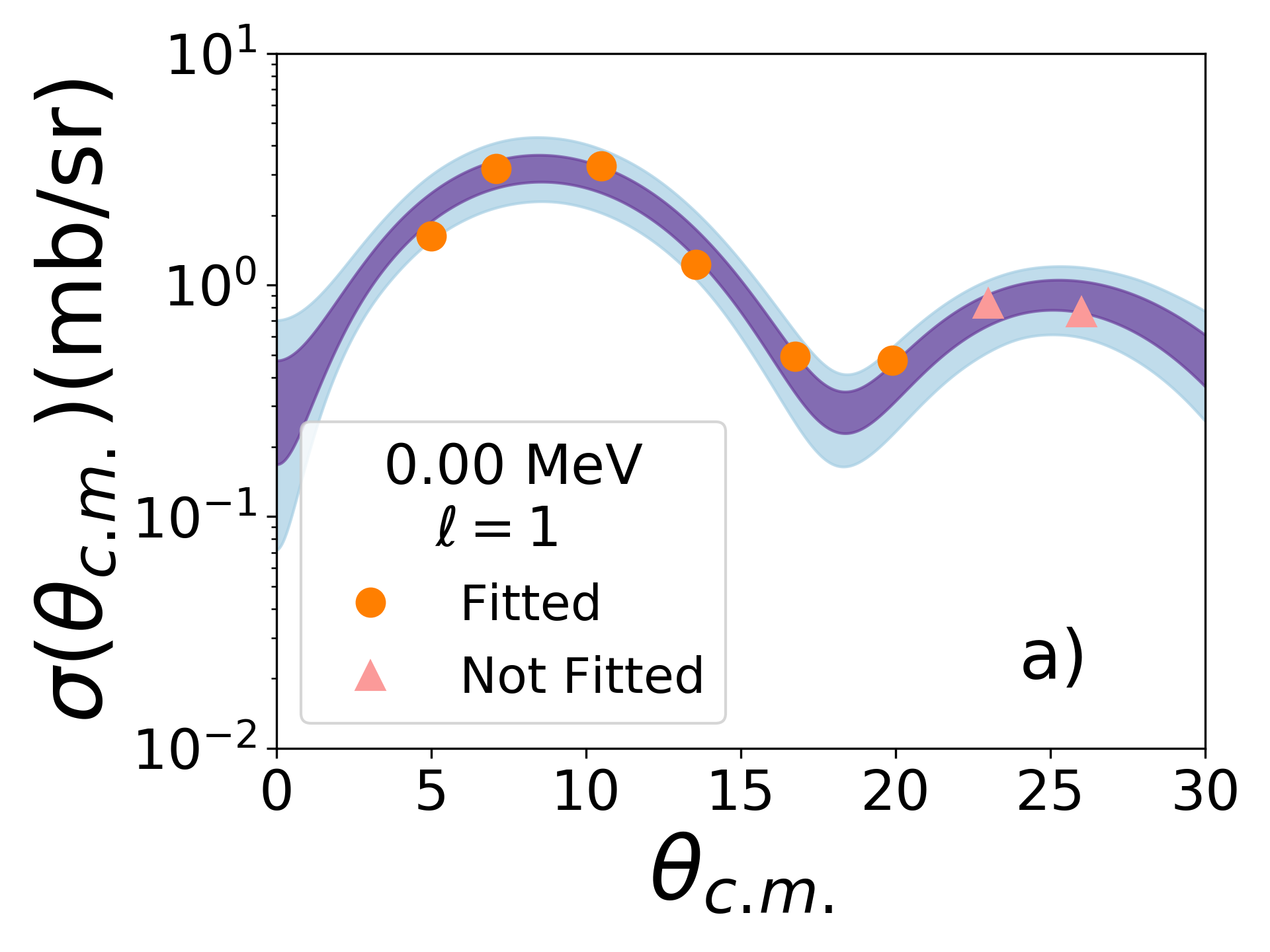
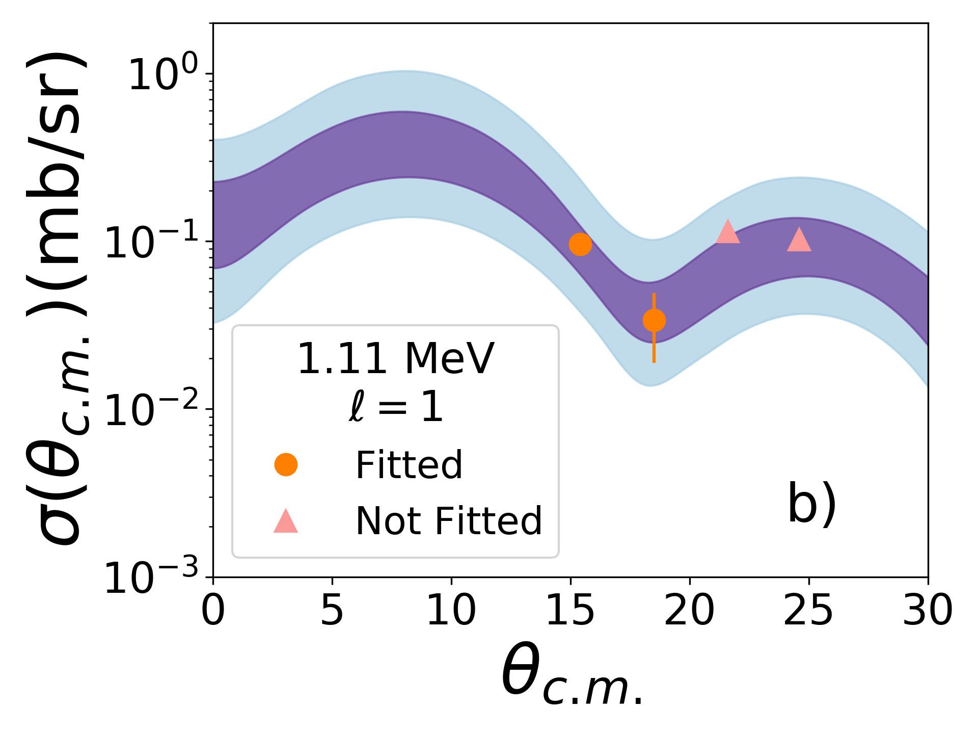
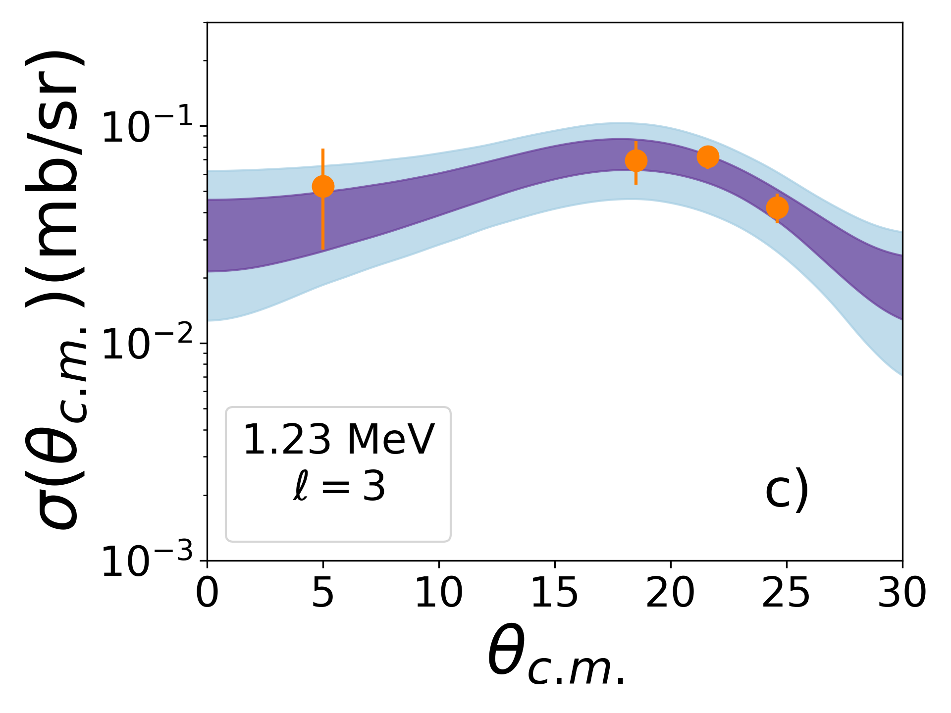
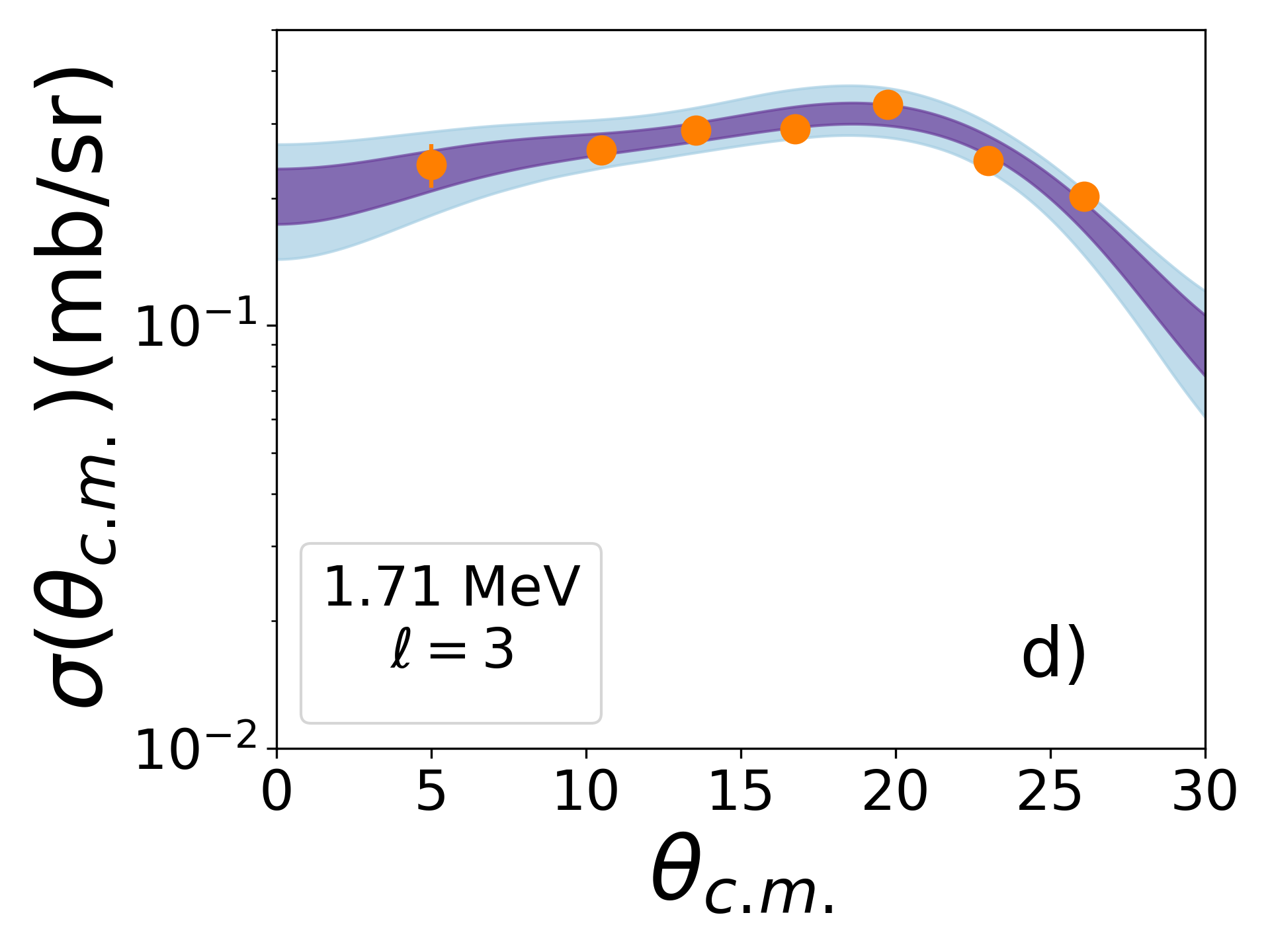
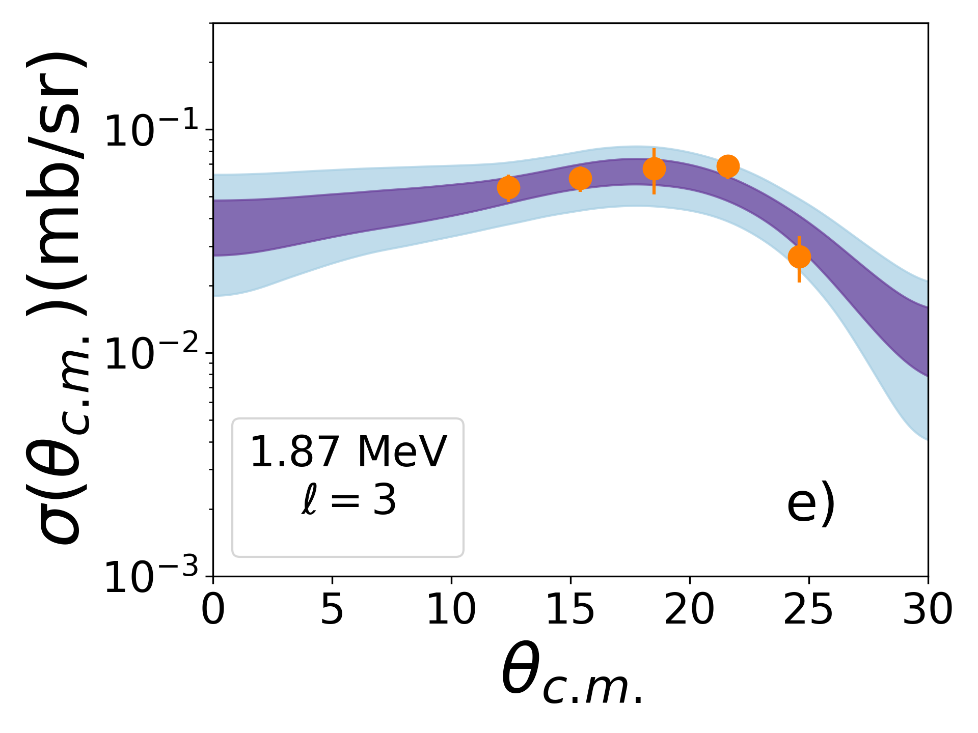
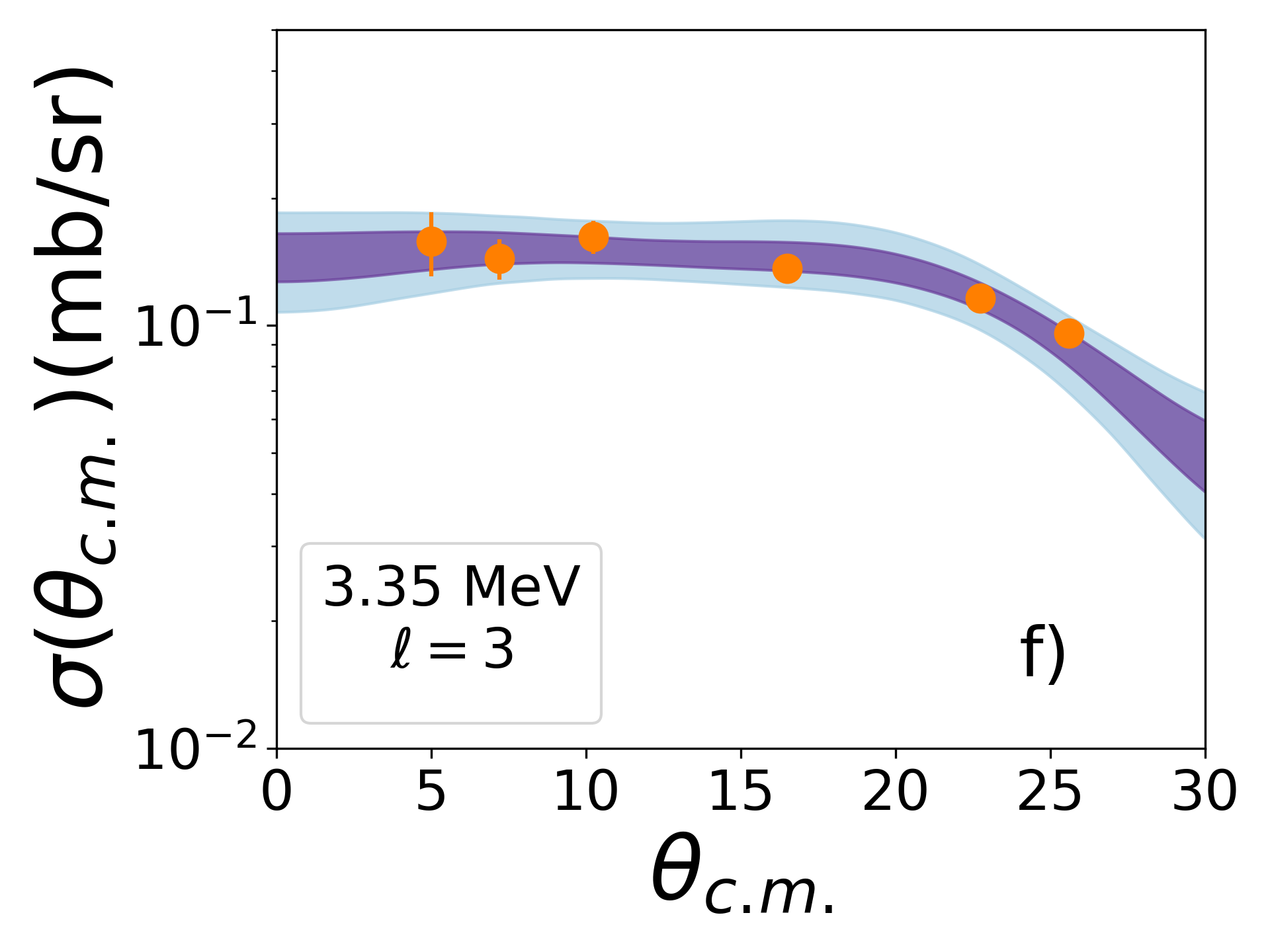
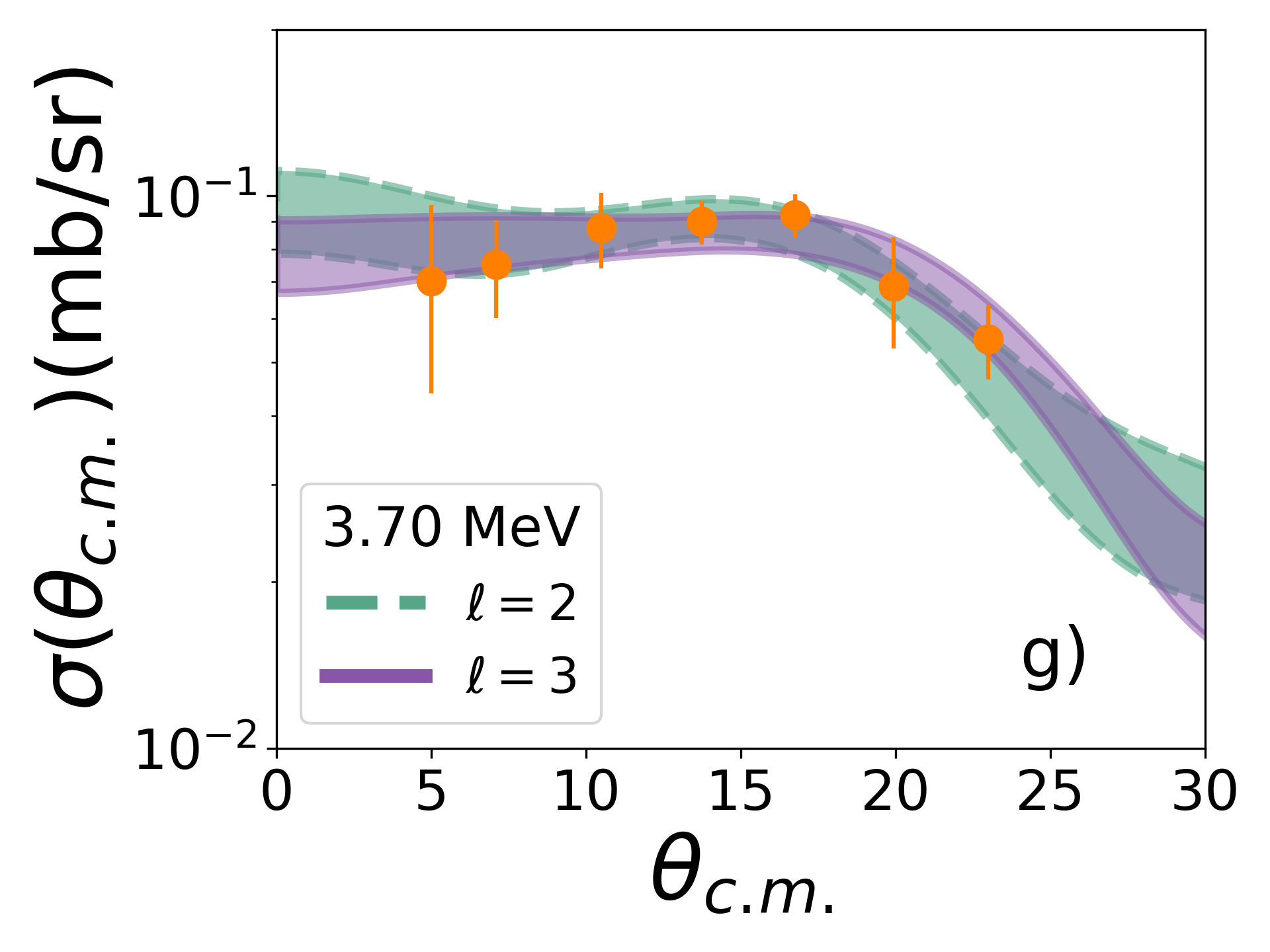
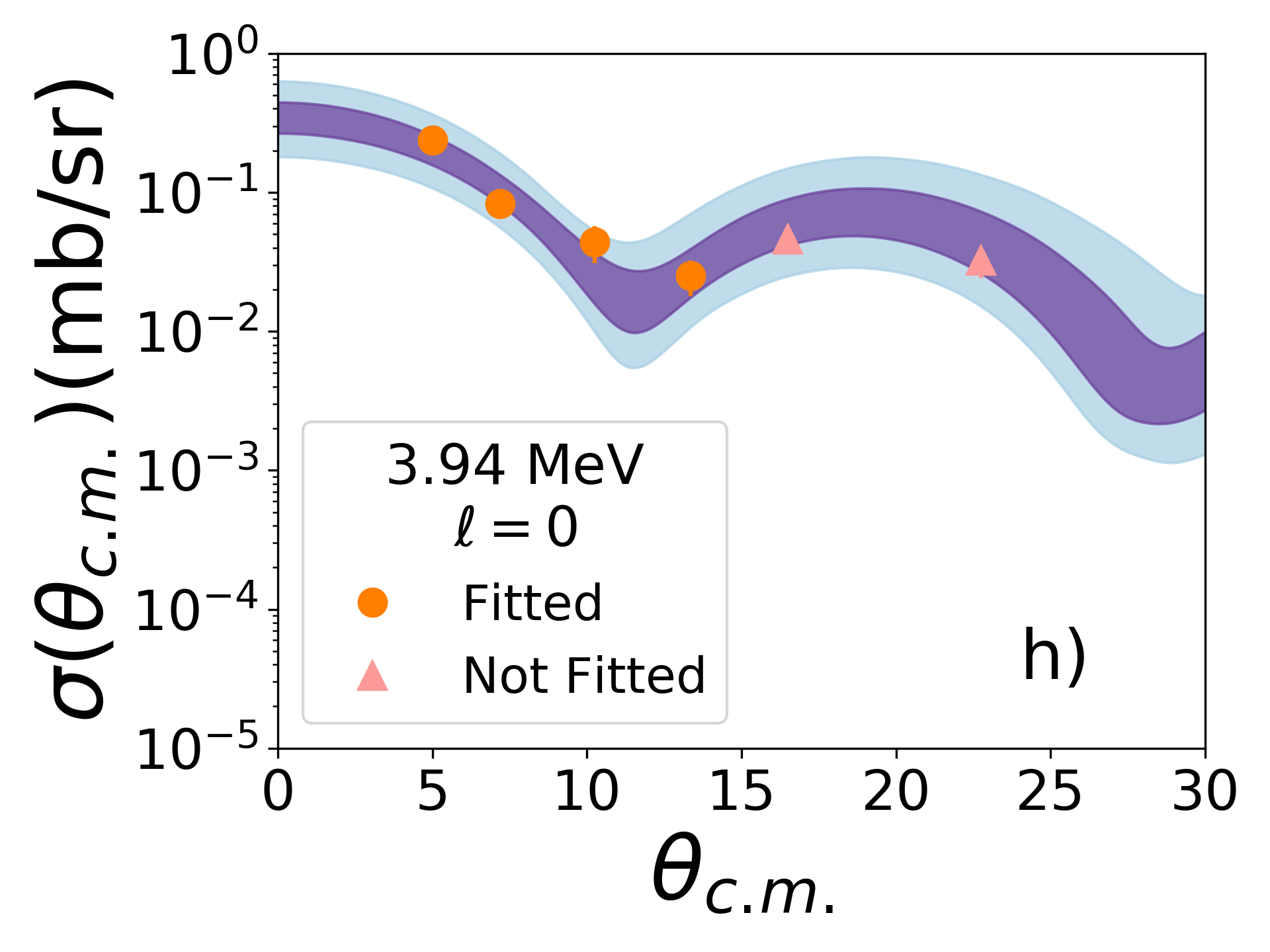
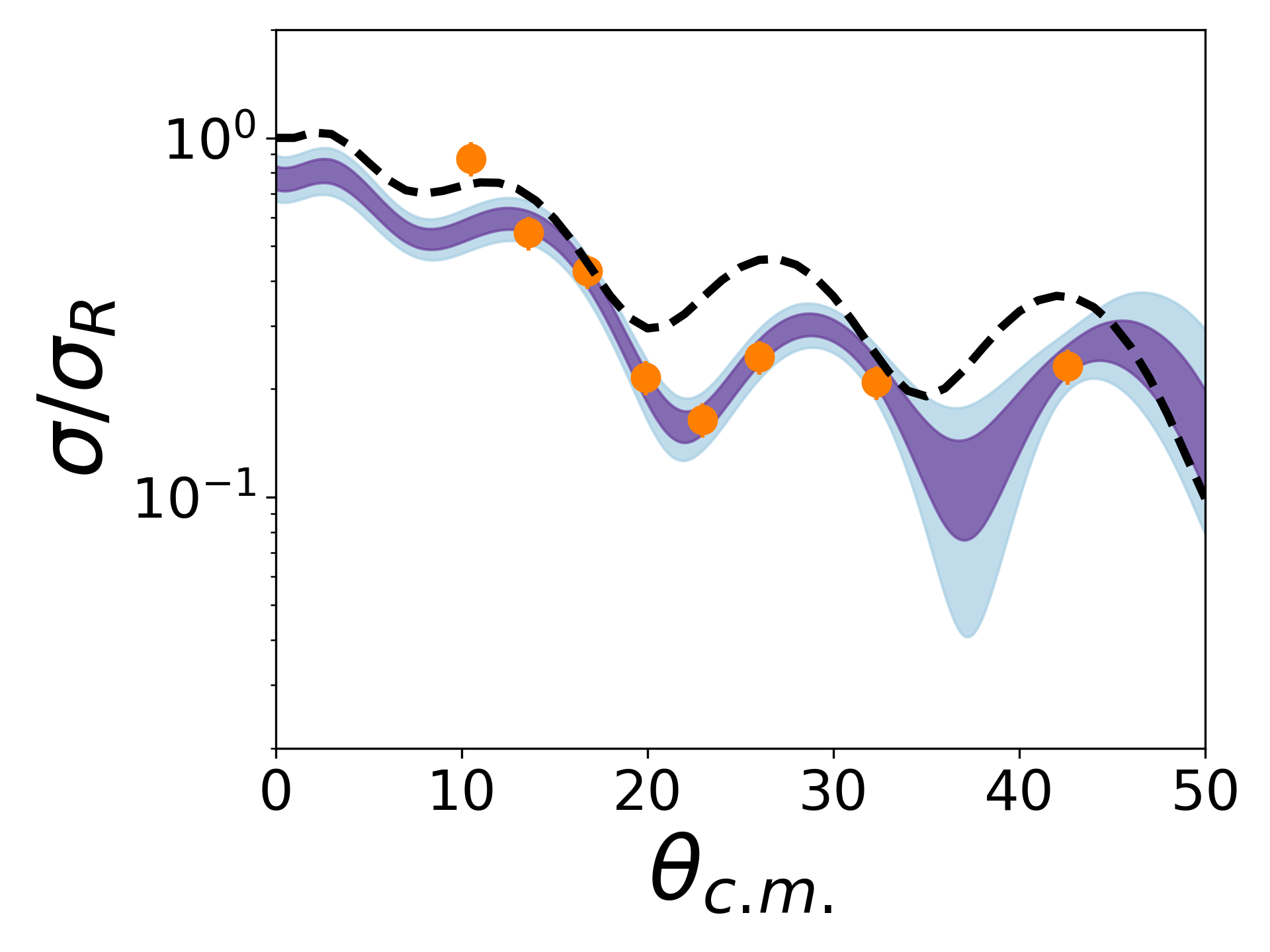
The Bayesian model of Sec. III allows us to extract spectroscopic factors and assign $\ell$ values to observed transfers, while taking into account uncertainties associated with the optical potentials. In order to test these methods, we will focus on a reanalysis of the ⁷⁰Zn$(d,^{3}$He$)^{69}$Cu reaction, which was originally presented in Ref. Morfouace et al. (2016). For reference, data was collected by impinging a $27$ MeV deuteron beam onto a thin target of enriched ⁷⁰Zn. The reaction products were measured with a magnetic spectrograph. The original study should be referred to for complete experimental details. This reaction and the measured data set have two important conditions that simplify our study. First, since ${}^{70}\textnormal{Zn}$ has a $0^{+}$ ground state, only a unique $\ell$ transfer is allowed for a given final state. Second, only 8 low lying bounds states were observed, meaning no additional theoretical model is needed for treating transfers to the continuum. Our results are summarized in Table 2. Comparisons are made to the original values of the zero-range and finite-range calculations of the previous work. Plots of the DWBA cross sections generated from the MCMC calculations are shown in Fig. 1. The purple and blue bands show the $68\%$ and $95\%$ credibility bands, respectively. Using samples directly from the Markov chain means that these credibility bands accurately account for all of the correlations present between the parameters. Each of these states will now be discussed in detail, with additional calculation details provided for the ground state in order to demonstrate the use of our Bayesian method.

Table 2: Summary of the spectroscopic factors derived in this work. Comparisons to the zero-range (ZR) and finite-range (FR) calculations of Ref. Morfouace et al. (2016) are made. All calculations use the same bound state parameters.

$E_{x}$(MeV)	$\ell$	$J^{\pi}$ a	$C^{2}S(ZR)$ Morfouace et al. (2016)	$C^{2}S(FR)$ Morfouace et al. (2016)	$C^{2}S$(This work)
$0.0$	$1$	$3/2^{-}$	$1.40(15)$	$1.50(17)$	$2.06^{+0.87}_{-0.68}$
$1.11$	$1$	$1/2^{-}$	-	$0.35(11)$	$0.48^{+0.52}_{-0.25}$
$1.23$	$3$	$(5/2^{-})$	$0.80(11)$	$0.70(10)$	$1.10^{+0.81}_{-0.48}$
$1.71$	$3$	$7/2^{-}$	$2.00(11)$	$2.50(14)$	$2.37^{+1.36}_{-0.84}$
$1.87$	$3$	$7/2^{-}$	$0.40(10)$	$0.50(10)$	$1.07^{+0.93}_{-0.51}$
$3.35$	$3$	$(7/2^{-})$	$1.60(10)$	$2.40(15)$	$2.67^{+1.83}_{-1.06}$
$3.70$	$2$	$(3/2^{+})$	$1.90(25)$	$1.50(20)$	$1.74^{+1.05}_{-0.62}$
	$3$	$(7/2^{-})$	-	-	$2.90^{+2.75}_{-1.43}$
$3.94$	$0$	$1/2^{+}$	$0.70(6)$	$0.70(10)$	$1.03^{+0.71}_{-0.44}$

• These assignments are discussed in depth in Sec. IV.1 through Sec. IV.7.

(a)

(b)

(c)

(d)

(e)

(f)

(g)

(h)

Figure 1: DWBA calculations for the states of ⁶⁹Cu . The $68\%$ and $95\%$ credibility intervals are shown in purple and blue, respectively. Only the data points shown in orange circles were considered in each calculation. For the $3.70$ MeV state the $68\%$ bands are shown for the two most likely $\ell$ transfers.

IV.1 Ground State

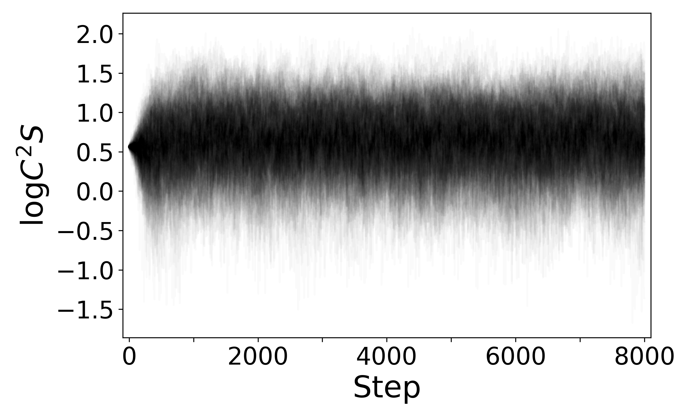
The MCMC calculations for the ground state were carried out using $8000$ steps and $400$ walkers in the ensemble. As an example we have provided the trace plot for the value of $C^{2}S$ as a function of step in Fig. 2. Parameter values were estimated by using the last $2000$ steps and thinning by $50$.

Figure 2: Trace of the MCMC walkers as a function of step and $\log(C^{2}S)$. Only the last 2000 steps were used for the posteriors.

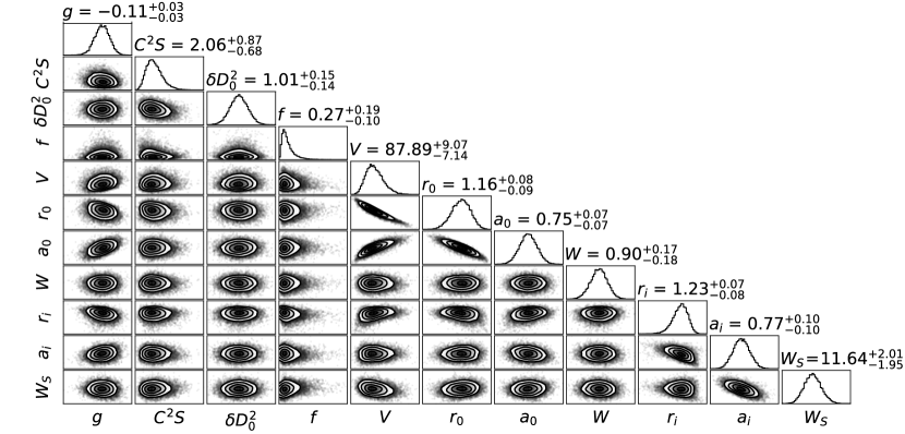
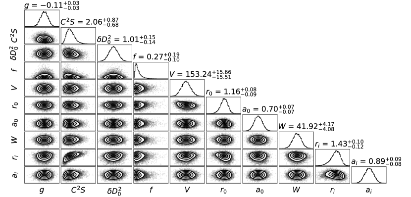
As noted before, all of our MCMC calculations simultaneously fit the elastic scattering and transfer data. This means that the posterior distributions shown in Fig. 4 are functions of both the elastic and ground state transfer data. The impacts of the choice of potential parameters and the scale parameter $\eta$ on the elastic fit is quite dramatic. If we were to adopt the global values in Table 1 without adjusting any parameters, the agreement between theory and experiment would be quite poor as shown by the dashed black line in Fig. 3. It should also be noted that the experimental uncertainties for these points are roughly $10\%$. On the other hand, the purple and blue bands in Fig. 3 show the fit obtained when we use our Bayesian model, which quite clearly provides a better description of the data. A significant difference is found between the normalization of the data and the optical model prediction, with $\eta\simeq 23\%$.

Figure 3: Bayesian fit of the elastic data calculated simultaneously with the $0.00$ MeV state. The $68\%$ and $95\%$ credibility intervals are shown in purple and blue respectively, while the black dashed curve was calculated using the global values from Table 1.

By examining the correlations between the parameters, our model should display the continuous ambiguity discussed in Sec. III.1. The pair-wise correlation plots in Fig. 4 show the posterior samples from the entrance (top) and exit (bottom) channel potentials and how they relate to those of $g$, $C^{2}S$, $\delta D_{0}$, and $f$. The intra-potential correlations are quite striking for the entrance channel. All of the real potential parameters, $V,r_{0},$ and $a_{0}$, show strong correlations with one another, and slightly weaker correlations existing between $V$, $r_{0}$, $r_{i}$, and $W_{s}$. Strong relationships also exist between $a_{i}$ and $W_{s}$, which is also another known continuous ambiguity Perey and Perey (1976). There is a much different situation for the exit potentials, where almost no intra-potential correlations are seen. This result is expected since there are no elastic scattering data to constrain these parameters and because the Bayesian model parameter $f$ limits the amount of information that can be drawn from the transfer channel data. However, there is a surprisingly strong relationship between the exit channel imaginary radius and $C^{2}S$. A similar relationship can be seen with the entrance channel imaginary radius, but the effects on $C^{2}S$ are dramatically less.

The results of the fit for the ground state are shown in Fig. 1(a). The circular orange data points were the only data considered in the fit in order to not bias our deduced spectroscopic factor as discussed in Sec. III.3. The ground state of ⁶⁹Cu is known to have a spin-parity of $\frac{3}{2}^{-}$, so the transfer was calculated assuming a $2p_{3/2}$ state.

Figure 4: The pair-wise correlation plots for the ground state transfer. The top plot shows the entrance potential parameters, while the bottom shows the exit channel parameters. Both channels are compared to the model parameters as defined in Eq. (III.3). The $68\%$ credibility intervals are listed at the top of each column with the dashed lines showing their relationship to the $1$-D parameter distributions. The plots were generated using the Python package corner Foreman-Mackey (2016).

IV.2 1.11 MeV State

The $1.11$ MeV state was only seen at four angles. Furthermore, only the first two data points lie within the first minimum. The $J^{\pi}=\frac{1}{2}^{-}$ assignment is based on the observed angular distributions of Ref. Zeidman and Nolen (1978) and the analyzing power measurement of Ref. Ajzenberg-Selove et al. (1981). In order to check that the data analyzed in the current work are consistent with these conclusions, the evidence integrals were calculated for $\ell=0,1,2$, and $3$ transfers using all the data points. The data support an $\ell=1$ transfer, but do not rule out an $\ell=3$ transfer. For this case, the median Bayes Factor defined in Eq. (11) is $B_{13}=6.32$ (i.e the fifty percentile of $Z_{1}/Z_{3}$), indicating that there is substantial evidence in favor of $\ell=1$. Since the data are consistent with the $\ell$ assignments of Ref. Ajzenberg-Selove et al. (1981, 1981), we carried out the MCMC calculations assuming a $2p_{1/2}$ state. The results of this calculation are plotted in Fig. 1(b).

IV.3 1.23 MeV State

The state located at $1.23$ MeV is definitely associated with an $\ell=3$ transfer. The previous analysis assumed a firm $J^{\pi}=\frac{5}{2}^{-}$; however, the literature does not provide direct evidence for this. The analyzing power of Ref. Ajzenberg-Selove et al. (1981) was inconclusive, and the authors suggested the presence of a doublet based on the observed width of the peak in the spectrum. The $(d,^{3}\textnormal{He})$ experiment of Ref. Zeidman and Nolen (1978) also suggested a doublet and noted the high spectroscopic factor obtained ($C^{2}S=1.5$) if a $\frac{5}{2}^{-}$ assignment was assumed. Other studies have also assigned a firm $J^{\pi}=\frac{5}{2}^{-}$ Franchoo et al. (2001); Stefanescu et al. (2008); Franchoo et al. (1998), but it is unclear if these results are actually independent determinations, or if they follow Table II of Ref. Zeidman and Nolen (1978). We therefore follow the ENSDF evaluation Nesaraja (2014) by recommending $J^{\pi}=(\frac{5}{2}^{-},\frac{7}{2}^{-})$, but only present the $C^{2}S$ value for $1f_{5/2}$ with the fit shown in Fig. 1(c).

IV.4 1.71 and 1.87 MeV States

From the parity constraints of Ref. Zeidman and Nolen (1978); Ajzenberg-Selove et al. (1981) and the $\gamma$-ray anisotropies observed in Ref. Ishii et al. (2000), a firm $J^{\pi}=\frac{7}{2}^{-}$ assignment has been made for the $1.71$ MeV state. The results from our DWBA fit for a $1f_{7/2}$ state are shown in Fig. 1(d). The arguments from the $1.71$ MeV state also apply to the state at $1.87$ MeV. A firm $J^{\pi}=\frac{7}{2}^{-}$ was assumed and a fit for a $1f_{7/2}$ state is shown in Fig. 1(e).

IV.5 3.35 MeV State

The state at $3.35$ MeV was reportedly seen in Ref. Zeidman and Nolen (1978), but no information was presented other than its possible existence. The previous analysis found an $\ell=3$ nature to the angular distribution, and made a tentative assignment of $J^{\pi}=(\frac{7}{2}^{-})$ assignment. Our methods support this conclusion as shown in Table 3. $B_{3\ell}>10$ for each other $\ell$ transition, indicating strong evidence for the $\ell=3$ transfer. The probability the final state was populated with an $\ell=3$ transfer is $P(\ell=3)=91^{+3}_{-4}\%$. However, DWBA is still unable to discriminate between $J^{\pi}=(\frac{5}{2}^{-},\frac{7}{2}^{-})$. Our fit assuming a $1f_{7/2}$ state is shown in Fig. 1(f).

Table 3: Results of the model comparison calculations for the $3.35$ and $3.70$ MeV states. For each $\ell$ value we list the $\log{Z}$ value calculated with nested sampling, the median Bayes factor when compared to the most likely transfer $\ell=3$, and the probability of each transfer.

	$\ell$	$\log{Z}_{\ell}$	$B_{3\ell}$	$P(\ell)$
$E_{x}=3.35$ MeV	0	3.856(330)	$>10^{4}$	$<.01\%$
	1	10.662(359)	$15.94$	$6^{+3}_{-2}\%$
	2	9.961(363)	$32.14$	$3^{+2}_{-1}\%$
	3	13.431(349)	1.0	$91^{+3}_{-4}\%$
$E_{x}=3.70$ MeV	0	10.393(365)	$>10^{3}$	$<0.02\%$
	1	14.947(351)	$45.98$	$2^{+1}_{-1}\%$
	2	16.640(346)	$8.47$	$10^{+5}_{-4}\%$
	3	18.776(336)	1.0	$88^{+4}_{-6}\%$

IV.6 3.70 MeV State

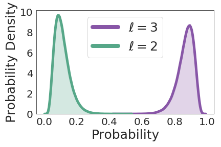
The state at $3.70$ MeV was also seen for the first time in Ref. Morfouace et al. (2016). However, our Bayesian method indicates an ambiguous $\ell$ assignment. As can be seen in Fig. 1(g), the measured angular distribution is relatively flat, and does not appear to differ from other states with $\ell=3$. However, an assignment of $\ell=2$ was made in the previous analysis. Comparing the evidence integral for each case, we indeed find the data effectively rule out $\ell=0$ and $1$, while supporting an $\ell=2$ or $3$ assignment. Looking at Table 3, we find a Bayes factor of $B_{32}=8.47$ for $\ell=3$ over $\ell=2$, which suggests substantial evidence in favor of the $\ell=3$ assignment. Using Eq. (12), the $68\%$ credibility intervals for the probabilities are $P(\ell=3)=88^{+4}_{-6}\%$ and $P(\ell=2)=10^{+5}_{-4}\%$, with the uncertainties coming from the statistical uncertainties of the nested sampling evidence estimation. The Kernel Densiy Estimates (KDE) for the two dominate transfers are shown in Fig. 5 Izenman (1991). Our fits for both $\ell=2$ and $3$ are shown if Fig. 1(g).

Figure 5: The KDE representations of the probabilities of the $\ell=2,3$ transfers for the 3.70 MeV state.

IV.7 3.94 MeV State

The $3.94$ MeV state was also observed for the first time in the previous study. The suggested $\ell=0$ assignment was found to be supported by the data. The second most likely transfer was found to be $\ell=1$. In this case $B_{01}=72.24$, indicating very strong evidence in favor of the $\ell=0$ assignment. The transfer to a $2s_{1/2}$ state is shown in Fig. 1(h).

V Discussion

V.1 Spectroscopic Factors

The results of the previous section merit closer examination, especially with regards to the spectroscopic factors. Comparing our results with those previously obtained in Table 2, two things are clear: our median values tend to be larger then Ref. Morfouace et al. (2016) and the uncertainties are much larger. To the first point, a majority of the shift comes from the lower value of $W_{s}$ used in the previous analysis. Though not stated in Ref. Morfouace et al. (2016), the surface potential was given a value of $W_{s}\approx 7.5$ MeV, which has the effect of lowering the value of $C^{2}S$. Our values on average are higher due to the Bayesian analysis favoring $W_{s}=11.93$ MeV and the inclusion of $\eta$, but these are somewhat offset due to the posterior values of $r_{i}$ and $a_{i}$ being lower than their global values. To the second point, when all of the sources of uncertainty are included in the analysis, we find highly asymmetric and data-driven uncertainties on $C^{2}S$ ranging from $35-108\%$. This is a substantial increase with regards to the common assumption that the extraction of spectroscopic factors comes with an approximately $25\%$ uncertainty Endt (1977). This may still be the case when the data are sufficiently informative, but the results of a single experiment should be viewed more conservatively. In particular, low angular coverage in the entrance channel elastic scattering data, the absence of any elastic scattering data in the exit channel, and transfer angular distributions with just a few points all play a role in final uncertainty that can be reported for $C^{2}S$.

To gain a clearer picture of the role each potential plays in the final uncertainty, the calculations for the ground state were repeated for the following cases:

1. Uncertainty in just the entrance channel potential parameters.

2. Uncertainty in both the entrance and exit channel potential parameters.

3. Uncertainty in the entrance, exit, and bound state potential parameters.

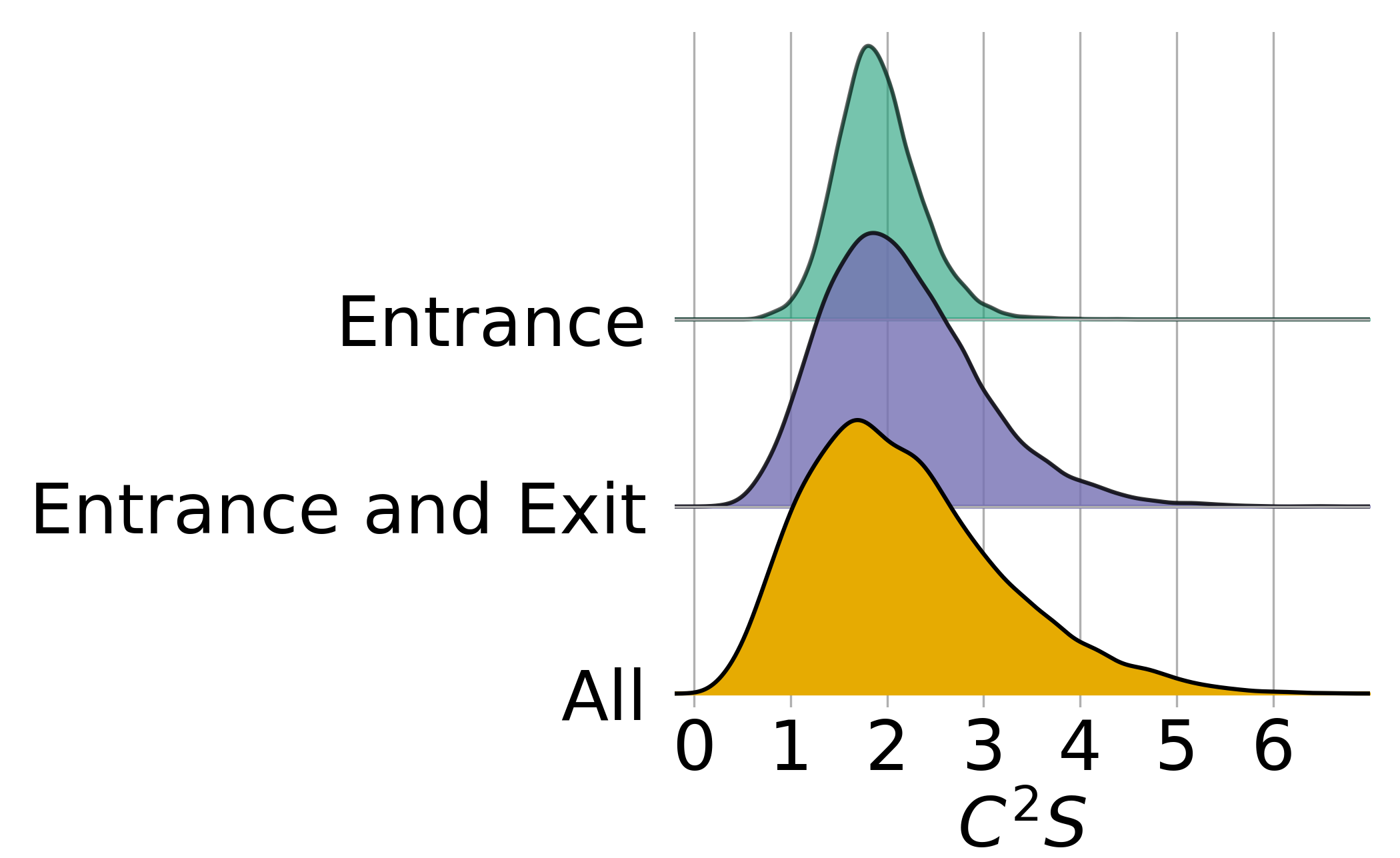
For case one we find the lowest uncertainty with $C^{2}S=1.88^{+0.44}_{-0.37}$ ($\approx\!24\%$). Case two is the same model used for all of the states in Sec. IV. This gives $C^{2}S=2.06^{+0.87}_{-0.68}$ ($\approx\!42\%$). Case three first requires that we specify the priors for the radius and diffuseness parameters of the bound state potential. Analogously to the exit channel, which also lacks data to directly constrain these parameters, we assign $V_{\textnormal{Bound}}\sim(\mu_{\textnormal{central},k},\{0.10\mu_{\textnormal{central},k}\}^{2})$. Again, $k$ is an index that runs over the radius and diffuseness parameters, and “central” refers to $r=1.25$ and $a=0.65$. This case has the largest final uncertainty with $C^{2}S=2.04^{+1.15}_{-0.85}$ ($\approx\!56\%$). The comparison between the final distribution for the spectroscopic factors obtained for just the entrance channel, entrance channel and exit channel, and all of the potentials including the bound state are shown in Fig. 6. This demonstrates the strong dependence of $C^{2}S$ on each of these potentials.

These results point toward ways to improve the precision of $C^{2}S$. Examination of the correlations in the posterior samples in Fig. 4 show that the imaginary radius in the exit channel is the parameter responsible for much of the uncertainty in $C^{2}S$. The samples for the exit channel also show little intra-potential correlation between the parameters. This is expected since the only data that could inform these parameters are in the transfer channel. If elastic data for the exit channel were available, then the proper parameter correlations could be inferred, thereby, reducing the uncertainty in the extracted spectroscopic factors. This could bring the uncertainty closer to the roughly $24\%$ seen in the case when just the entrance potential is considered.

Bound state parameter dependence could have significant impact on astrophysical applications as well. In these applications, the extraction of $C^{2}S$ is an intermediate step towards calculation of quantities relevant to astrophysics such as particle partial widths and direct capture cross sections. It was noted in Ref. Bertone et al. (2002) that it is essential to use the same bound state parameters for both the extraction of $C^{2}S$ and calculation of the direct capture cross section or partial width. This procedure was found to significantly reduce the final uncertainties on these quantities. If the bound state parameters are included in a Bayesian model to extract $C^{2}S$, then it becomes possible to calculate these quantities not only using the same bound state parameters, but using fully correlated, statistically meaningful samples informed directly by the transfer reaction measurement. Future work should investigate the effectiveness and impact of determining partial widths and direct capture cross sections using a Bayesian framework.

Figure 6: Ridge line plot that compares the KDE distributions for the ground state $C^{2}S$ when there is variation in the entrance potential; entrance and exit potentials; and in the entrance, exit, and bound state potentials. The percentage uncertainties go from $24\%$, $42\%$, and $56\%$, respectively.

V.2 Nuclear Structure of ${}^{69}\textnormal{Cu}$

Structure properties of ${}^{69}\textnormal{Cu}$ are also influenced by our results. The occupancy of orbitals tends to be higher than expected for both the open $pf$ orbitals and for the closed $1f_{7/2}$ proton shell. In order to propagate the uncertainties from each $C^{2}S$, we use the MCMC samples to construct a KDE for each state. From these densities we pull $10^{5}$ samples to estimate the occupancy:

$$n=\sum_{i}^{N}C^{2}S_{i},$$ (25)

where $i$ refers to each of the $N$ states considered in the sum. Similarly, the energy of the $1f_{7/2}$ shell can be determined from:

$$E(1f_{7/2})=\frac{\sum_{i}^{N}C^{2}S_{i}(1f_{7/2})E_{i}(1f_{7/2})}{n_{1f_{7/2}}}.$$ (26)

The occupancy above the closed shell was found to be $n_{pf}=3.90^{+1.03}_{-1.28}$, which is consistent but systematically higher than the value of $2.55(23)$ from the finite range calculations of the previous analysis. For the $1f_{7/2}$ shell we have two scenarios dependent on the identity of the state at $3.70$ MeV. If the state does not belong to the $f$ shell, we have $n_{1f_{7/2}}=6.64^{+2.47}_{-1.79}$ and $E(1f_{7/2})=2.43^{+0.23}_{-0.25}$ , or if it does, $n_{1f_{7/2}}=10.03^{+3.63}_{-2.66}$ and $E(1f_{7/2})=2.86^{+0.23}_{-0.26}$. Looking at the median value for $n_{pf}$, we would expect $n_{1f_{7/2}}=6.10$. This may point to the $\ell=2$ assignment of the $3.70$ MeV state being the correct one, but it must be recognized that there are still large uncertainties on all of these quantities. Furthermore, since the optical model parameters are shared by these states, these derived values are susceptible to significant systematic shifts. In light of this fact, these credibility intervals should be viewed as approximations. Perhaps more importantly is that if the $3.70$ state belongs to the $1f_{7/2}$, then the full strength of this shell has been observed. The shell model calculations in Ref. Morfouace et al. (2016) predict a much higher energy than $E(1f_{7/2})=2.86$ due to the presence of more states at higher excitation energies. A future experiment with a higher incident beam energy that would be capable of populating these predicted higher lying states could help clarify these discrepancies.

V.3 Comparison to Other Bayesian Studies

It is also worthwhile to compare our methods with those of several recent publications, which have also applied Bayesian methods to optical potentials Lovell and Nunes (2018); King et al. (2019). These papers differ from our approach in a few key ways: the data come from multiple experiments, exit and entrance channels are fitted separately, transfers are calculated using finite range effects, and the prior distributions are much wider than ours ($100\%$ of the initial global values). In a fully Bayesian framework, fitting the data in the entrance and exit channels separately or simultaneously is equivalent as long as the same model is used S Sivia and Skilling (2006). While our priors are narrower, they could likely be made broader if there was elastic scattering data over a wider range of angles. Full finite-range calculations could be important to include in future studies, but, as seen in Table 2, for this reaction the average difference is roughly $16\%$, well within the uncertainty arising from the optical potentials. Including these effects will require a more efficient way to evaluate the likelihood function. Specifically, a finite-range calculation takes roughly $50$ times longer than a calculation using the zero-range approximation. For this work $2\times 10^{6}$ likelihood evaluations took approximately $22$ hours, meaning the finite-range calculation would take over $1000$ hours. As well as those differences, our results differ from those of Ref.King et al. (2019) in one important aspect. Here, we confirmed the strong correlations between optical model parameters that are expected from historical studies Hodgson (1971), and treat them in a statistically meaningful way. We stress that our method does not assume these correlations, but that they appear to be a consequence of the Wood-Saxon potential form factor. On the other hand, in their comparison of frequentist and Bayesian methods Ref.King et al. (2019) do not observe such correlations, with the exception of the $V_{0}$ and $r_{0}$ anti-correlation, and ascribe their finding to the non-Gaussian posterior distributions, which would be poorly described by the frequentist model. We do not know the origin of this disagreement, and suggest that it should be investigated further.

VI Conclusions

In this paper we have presented a method to calculate uncertainties in spectroscopic factors and angular momentum assignments that include the uncertainty of the nuclear optical model parameters by using Bayesian inference. We find that for the ${}^{70}\textnormal{Zn}(d,^{3}\textnormal{He})^{69}\textnormal{Cu}$ data analyzed here, spectroscopic factors are subject to large uncertainties that can approach $100\%$. If the exit channel elastic scattering is measured, this uncertainty could be reduced significantly due to the high correlation between the exit channel imaginary radius and the spectroscopic factor. Application of Bayesian model selection also found that there is substantial evidence in the data to suggest an $\ell=3$ transfer for the $3.70$ MeV state, which differs from the previous conclusion of an $\ell=2$ assignment. Further work is needed to resolve the ambiguity of this state. We also find that the Bayesian approach confirms the highly correlated nature of the optical model potential parameters. The application of these techniques to other data sets and global potentials could significantly improve the ability of future works to accurately assign uncertainties to calculations involving the optical model.

Appendix A: Potential Ambiguities for ${}^{70}\textnormal{Zn}(d,d)^{70}\textnormal{Zn}$

As discussed in Sec. III.1, the continuous and discrete ambiguities pose serious issues to any uncertainty quantification of optical model potentials. It is worthwhile to demonstrate that these issues occur naturally in our data set, and that they are not consequences of the Bayesian methods developed throughout this paper. We do this by using artificially generated data that possess the same characteristics of our measured data points. In particular, we use limited angular coverage, $\theta_{c.\!m.}\leq 50^{\circ}$, and equivalent statistical uncertainties of $10\%$. The data are generated by randomly perturbing the theoretical cross section from FRESCO according to:

$$\frac{d\sigma}{d\Omega}_{\textnormal{Artificial},i}=\frac{d\sigma}{d\Omega}_{\textnormal{Fresco},i}+\epsilon_{i},$$ (27)

where $i$ refers to the center of mass angle and $\epsilon_{i}$ is defined as

$$\epsilon_{i}\sim\mathcal{N}\bigg{(}0,\bigg{(}0.10\,\frac{d\sigma}{d\Omega}_{\textnormal{Fresco},i}\bigg{)}^{2}\bigg{)}.$$ (28)

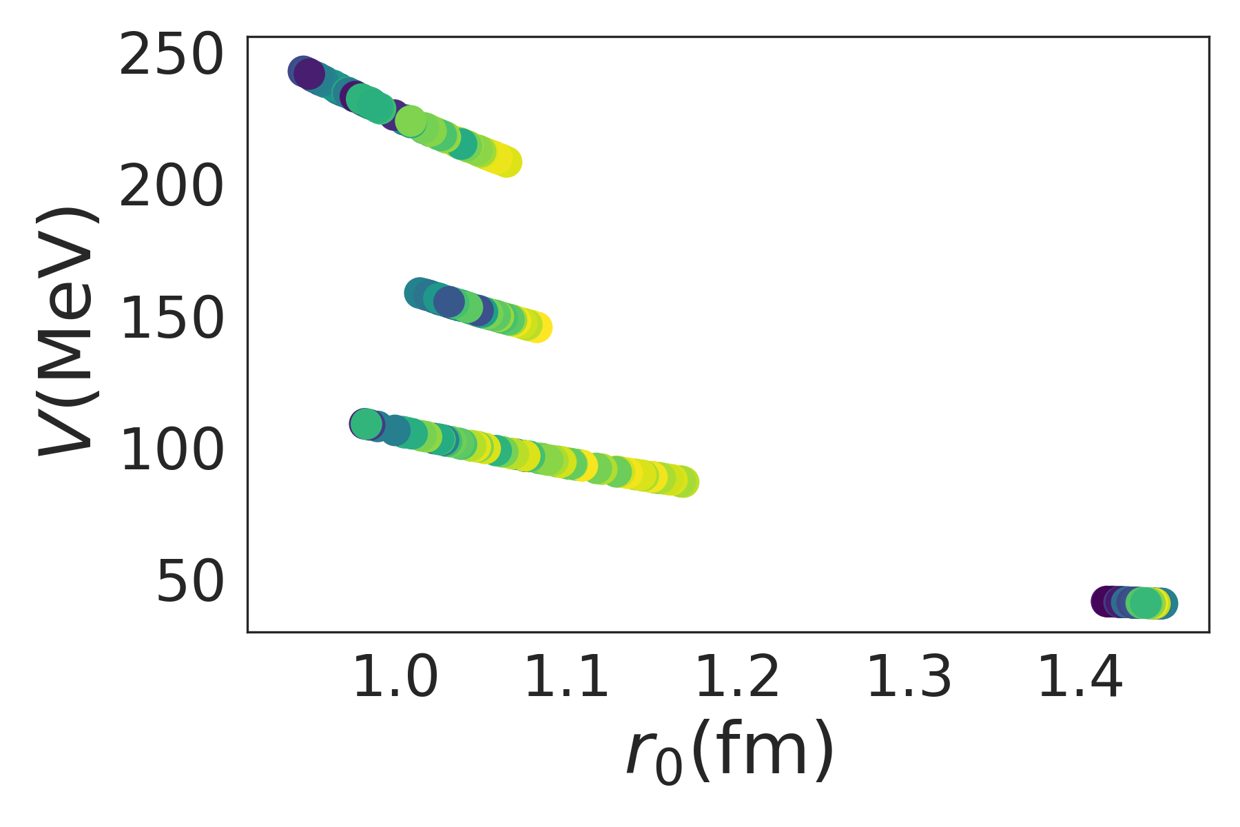
Using a maximum likelihood estimate, 4 different values were used for the real potential, $V=40,80,150,200$ MeV. For each of these starting values 100 minimization runs were performed, with each run consisting of a minor perturbation of all of the starting parameters. This procedure effectively probes the continuous ambiguity for each family of $V$. These results are plotted in Fig. 7, which shows each solution’s value of $V$ and $r_{0}$. Their color is based on the minimized value, with the least likely being darker and the most likely being brighter. This result shows that the two ambiguities will be present even in an idealized situation, and that any effort to quantify uncertainties must be able to address the issues they create.

Figure 7: The $V$ and $r$ values from the exploration of the maximum likelihood solutions. The colors correspond to the likelihood values. As the colors get brighter, the values become more likely. The continuous and discrete ambiguity can bee seen clearly.

Appendix B: $a$ parameter for Ensemble Sampling

As mentioned in the main text, all of our MCMC calculations used an ensemble sampler with a stretch move parameter set to $a=2$. We now detail the meaning of this parameter as defined in Ref. Goodman and Weare (2010).

A single step of the entire ensemble is taken by updating the positions for each walker individually. The stretch move does this for a walker $k$ by selecting at random another walker from the ensemble and proposing an update of the form:

$$X_{k}(t)\rightarrow Y=X_{j}+z(X_{k}(t)-X_{j}),$$ (29)

where $X_{k}(t)$ is the position of walker $k$ at step $t$, $X_{j}$ is the position of the randomly selected walker in the ensemble ($k\neq j$), and $z$ is a scaling variable drawn from the distribution $g(z)$. This distribution is defined by the single free parameter, $a$, and is given by the function:

$$g(z)\propto\begin{cases}\frac{1}{\sqrt{z}}&\textnormal{if}\,z\in[\frac{1}{a},a],\\ 0&\textnormal{otherwise}.\end{cases}$$ (30)

The proposed position $Y$ in a parameter space of $N$ dimensions is then accepted with probability:

$$q=\textnormal{min}\bigg{(}1,z^{N-1}\frac{p(Y)}{p(X_{k}(t))}\bigg{)}.$$ (31)

It is possible to improve the performance of the sampler by adjusting $a$. Lower values will tend to increase the number of accepted proposals, while higher values will tend to decrease them. All calculations in this work had acceptance fractions between $0.2$ and $0.5$, indicating the choice of $a=2$ was adequate Foreman-Mackey et al. (2013).

Appendix C: Description of Nested Sampling

We give a brief overview of the nested sampling algorithm here, but Ref. Speagle (2019); Skilling (2006, 2004) should be consulted for a more detailed explanation. The idea of nested sampling is to estimate the evidence by defining a prior mass, $X$, defined by an integral over the priors, $P(\theta)$, with respect to the likelihood, $\mathcal{L}$:

$$X(\lambda)=\int_{\mathcal{L}>\lambda}P(\theta)d\theta.$$ (32)

As $\lambda$ increases, $X$ decreases from $1$ to $0$. This definition allows the evidence integral to be written:

$$Z=\int_{0}^{1}\mathcal{L}(X)dX\approx\sum_{i=1}^{m}\frac{1}{2}(X_{i-1}-X_{i+1})\mathcal{L}_{i},$$ (33)

where the sum comes from the application of the trapezoid rule. The quantity $\frac{1}{2}(X_{i-1}-X_{i+1})$ is also referred to as the weight, $w_{i}$. Thus, the algorithm becomes:

1. Set $Z_{0}=0$ and $X_{0}=1$.

2. Draw $n$ live points from the prior distributions.

3. Select the live point with the lowest value of $\mathcal{L}_{i}$, and calculate $\ln X_{i}\approx\frac{i+\sqrt{i}}{n}$.

4. Add the weighted sample $\mathcal{L}_{i}w_{i}$ to $Z$.

5. Update the selected live point by drawing a new point from the prior satisfying $\mathcal{L}_{i+1}\geq\mathcal{L}_{i}$.

6. Repeat.

The number of samples, $m$, required for an accurate determination of $Z$ can be estimated from the upper bound at a step by: $\Delta Z_{i}\approx\mathcal{L}_{\textnormal{max}}X_{i}$, where $\mathcal{L}_{\textnormal{max}}$ is the highest likelihood value of the remaining live points.

References

- Feshbach (1958) H. Feshbach, Annals of Physics 5, 357 (1958).
- Macfarlane and French (1960) M. H. Macfarlane and J. B. French, Rev. Mod. Phys. 32, 567 (1960).
- Satchler (1983) G. R. Satchler, Direct nuclear reactions (1983).
- Bardayan (2016) D. W. Bardayan, Journal of Physics G: Nuclear and Particle Physics 43, 043001 (2016).
- Wimmer (2018) K. Wimmer, Journal of Physics G: Nuclear and Particle Physics 45, 033002 (2018).
- Varner et al. (1991) R. Varner, W. Thompson, T. McAbee, E. Ludwig, and T. Clegg, Physics Reports 201, 57 (1991).
- Endt (1977) P. Endt, Atomic Data and Nuclear Data Tables 19, 23 (1977).
- Lovell and Nunes (2015) A. E. Lovell and F. M. Nunes, Journal of Physics G: Nuclear and Particle Physics 42, 034014 (2015).
- Lovell et al. (2017) A. E. Lovell, F. M. Nunes, J. Sarich, and S. M. Wild, Phys. Rev. C 95, 024611 (2017).
- King et al. (2018) G. B. King, A. E. Lovell, and F. M. Nunes, Phys. Rev. C 98, 044623 (2018).
- Lovell and Nunes (2018) A. E. Lovell and F. M. Nunes, Phys. Rev. C 97, 064612 (2018).
- King et al. (2019) G. B. King, A. E. Lovell, L. Neufcourt, and F. M. Nunes, Physical Review Letters 122 (2019), 10.1103/PhysRevLett.122.232502.
- Morfouace et al. (2016) P. Morfouace, S. Franchoo, K. Sieja, I. Stefan, N. de Séréville, F. Hammache, M. Assié, F. Azaiez, C. Borcea, R. Borcea, L. Grassi, J. Guillot, B. Le Crom, L. Lefebvre, I. Matea, D. Mengoni, D. Napoli, C. Petrone, M. Stanoiu, D. Suzuki, and D. Testov, Phys. Rev. C 93, 064308 (2016).
- Becchetti and Greenlees (1969a) F. D. Becchetti and G. W. Greenlees, Phys. Rev. 182, 1190 (1969a).
- Hodgson (1971) P. Hodgson, Nuclear reactions and nuclear structure, International series of monographs on physics (Clarendon Press, 1971).
- (16) I. J. Thompson, “Fresco coupled reaction channels calculations,” Unpublished.
- Perey and Perey (1976) C. Perey and F. Perey, Atomic Data and Nuclear Data Tables 17, 1 (1976).
- Becchetti and Greenlees (1969b) F. D. Becchetti and G. W. Greenlees, Phys. Rev. 182, 1190 (1969b).
- Beccehetti and Greenless (1969) F. D. Beccehetti and G. W. Greenless, University of Minnesota , 116 (1969).
- Pang et al. (2009) D. Y. Pang, P. Roussel-Chomaz, H. Savajols, R. L. Varner, and R. Wolski, Phys. Rev. C 79, 024615 (2009).
- Daehnick et al. (1980) W. W. Daehnick, J. D. Childs, and Z. Vrcelj, Phys. Rev. C 21, 2253 (1980).
- Thompson and Nunes (2009) I. J. Thompson and F. M. Nunes, Nuclear Reactions for Astrophysics: Principles, Calculation and Applications of Low-Energy Reactions (Cambridge University Press, 2009).
- Lee et al. (1964) L. L. Lee, J. P. Schiffer, B. Zeidman, G. R. Satchler, R. M. Drisko, and R. H. Bassel, Phys. Rev. 136, B971 (1964).
- (24) P. Kunz, “Zero range distorted wave born approximation,” Unpublished.
- Bassel (1966) R. H. Bassel, Phys. Rev. 149, 791 (1966).
- Goldfarb et al. (1973) L. Goldfarb, J. Gonzalez, and A. Phillips, Nuclear Physics A 209, 77 (1973).
- Bertone et al. (2002) P. F. Bertone, A. E. Champagne, M. Boswell, C. Iliadis, S. E. Hale, V. Y. Hansper, and D. C. Powell, Phys. Rev. C 66, 055804 (2002).
- Brida et al. (2011) I. Brida, S. C. Pieper, and R. B. Wiringa, Phys. Rev. C 84, 024319 (2011).
- S Sivia and Skilling (2006) D. S Sivia and J. Skilling, Data Analysis A Bayesian Tutorial (2006).
- Jeffreys (1961) H. Jeffreys, Theory of Probability, 3rd ed. (Oxford, Oxford, England, 1961).
- Vernotte et al. (1982) J. Vernotte, G. Berrier-Ronsin, J. Kalifa, and R. Tamisier, Nuclear Physics A 390, 285 (1982).
- Drisko et al. (1963) R. Drisko, G. Satchler, and R. Bassel, Physics Letters 5, 347 (1963).
- Hodgson (1994) P. E. Hodgson, The nucleon optical model (World Scientific, 1994).
- Perey (1963) F. G. Perey, Phys. Rev. 131, 745 (1963).
- Bjorklund and Fernbach (1958) F. Bjorklund and S. Fernbach, Phys. Rev. 109, 1295 (1958).
- Perey and Perey (1963) C. M. Perey and F. G. Perey, Phys. Rev. 132, 755 (1963).
- Schiffer et al. (2012) J. P. Schiffer, C. R. Hoffman, B. P. Kay, J. A. Clark, C. M. Deibel, S. J. Freeman, A. M. Howard, A. J. Mitchell, P. D. Parker, D. K. Sharp, and J. S. Thomas, Phys. Rev. Lett. 108, 022501 (2012).
- Sharma (2017) S. Sharma, Annual Review of Astronomy and Astrophysics 55, 213 (2017), https://doi.org/10.1146/annurev-astro-082214-122339 .
- Goodman and Weare (2010) J. Goodman and J. Weare, Communications in Applied Mathematics and Computational Science 5, 65 (2010).
- Foreman-Mackey et al. (2013) D. Foreman-Mackey, D. W. Hogg, D. Lang, and J. Goodman, Publications of the Astronomical Society of the Pacific 125, 306 (2013), arXiv:1202.3665 [astro-ph.IM] .
- Skilling (2006) J. Skilling, Bayesian Anal. 1, 833 (2006).
- Skilling (2004) J. Skilling, in American Institute of Physics Conference Series, American Institute of Physics Conference Series, Vol. 735, edited by R. Fischer, R. Preuss, and U. V. Toussaint (2004) pp. 395–405.
- Speagle (2019) J. S. Speagle, “dynesty: A dynamic nested sampling package for estimating bayesian posteriors and evidences,” (2019), arXiv:1904.02180 [astro-ph.IM] .
- Foreman-Mackey (2016) D. Foreman-Mackey, Journal of Open Source Software 1, 24 (2016).
- Zeidman and Nolen (1978) B. Zeidman and J. A. Nolen, Phys. Rev. C 18, 2122 (1978).
- Ajzenberg-Selove et al. (1981) F. Ajzenberg-Selove, R. E. Brown, E. R. Flynn, and J. W. Sunier, Phys. Rev. C 24, 1762 (1981).
- Franchoo et al. (2001) S. Franchoo, M. Huyse, K. Kruglov, Y. Kudryavtsev, W. F. Mueller, R. Raabe, I. Reusen, P. Van Duppen, J. Van Roosbroeck, L. Vermeeren, A. Wöhr, H. Grawe, K.-L. Kratz, B. Pfeiffer, and W. B. Walters, Phys. Rev. C 64, 054308 (2001).
- Stefanescu et al. (2008) I. Stefanescu, G. Georgiev, D. L. Balabanski, N. Blasi, A. Blazhev, N. Bree, J. Cederkäll, T. E. Cocolios, T. Davinson, J. Diriken, J. Eberth, A. Ekström, D. Fedorov, V. N. Fedosseev, L. M. Fraile, S. Franchoo, K. Gladnishki, M. Huyse, O. Ivanov, V. Ivanov, J. Iwanicki, J. Jolie, T. Konstantinopoulos, T. Kröll, R. Krücken, U. Köster, A. Lagoyannis, G. Lo Bianco, P. Maierbeck, B. A. Marsh, P. Napiorkowski, N. Patronis, D. Pauwels, G. Rainovski, P. Reiter, K. Riisager, M. Seliverstov, G. Sletten, J. Van de Walle, P. Van Duppen, D. Voulot, N. Warr, F. Wenander, and K. Wrzosek, Phys. Rev. Lett. 100, 112502 (2008).
- Franchoo et al. (1998) S. Franchoo, M. Huyse, K. Kruglov, Y. Kudryavtsev, W. F. Mueller, R. Raabe, I. Reusen, P. Van Duppen, J. Van Roosbroeck, L. Vermeeren, A. Wöhr, K.-L. Kratz, B. Pfeiffer, and W. B. Walters, Phys. Rev. Lett. 81, 3100 (1998).
- Nesaraja (2014) C. Nesaraja, Nuclear Data Sheets 115, 1 (2014).
- Ishii et al. (2000) T. Ishii, M. Asai, A. Makishima, I. Hossain, M. Ogawa, J. Hasegawa, M. Matsuda, and S. Ichikawa, Phys. Rev. Lett. 84, 39 (2000).
- Izenman (1991) A. J. Izenman, Journal of the American Statistical Association 86, 205 (1991).