Fluid Flow on Vegetated Hillslope

Abstract

In this paper, we present a deduction of swallow water equations in the presence of vegetation based on spatial averaging techniques starting from the general principles of conservation of mass and momentum. For this purpose, we worked in the hydrostatic approximation of the pressure field and we considered certain hypotheses of kinematic and topographical nature and assumptions on the structure of the vegetation. Some elements of differential geometry necessary to facilitate the reading of the paper can be found in the Appendix.
Keywords: swallow water equations, non-homogeneous hyperbolic system, hydrological process, averaging method, porosity.
2010 MSC: 35Q35, 35L60, 76S99, 53Z05.

1 Introduction

The presence of plants on the hill creates a resistance force to the water flow and influences the process of water accumulation on the soil surface. The large diversity of plants growing on a hill makes the elaboration of an unitary model of the water flow over a soil covered by vegetation very difficult. Here, we present a model based on water mass and momentum balance equations that takes into account the presence of certain type of plants.

More precisely, the plants form a dense net of rigid vertical tubes and the water fills the “voided” space up to a level not higher than these plant tubes, see Figure 1.

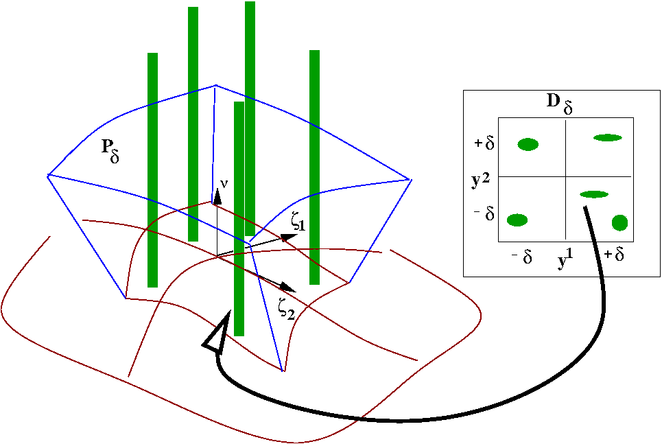
Figure 1: The representative element of the volume $P_{\delta}$ used for mediation. The bottom surface of $P_{\delta}$ has a representative width $\delta$ along two orthogonal directions on this surface. The water depth $h$ associated to $P_{\delta}$ is the averaged value of the physical water depth $\widetilde{h}$ inside $P_{\delta}$.

The article is structured as follows. A full hyperbolic PDE model obtained by averaging the equations for the conservation of mass and momentum is presented in Section 2. Some closure relations for these balance equations can be found in Section 3, while some mathematical properties of this model are pointed out in Section 4. For practical purposes, a simplified model that preserves the properties of the general model is also considered in this last section. The Appendix is dedicated to some elements of differential geometry used throughout the paper.

2 Space Averaging Models

Space averaging is a method to define a unique continuous model associated to a heterogeneous fluid-solid mechanical system. The method is largely used in porous soil media models [2, 7, 14]. For the fluid-plant physical system, the porous analogy was also used in [1, 9, 11], especially in the case of submerged vegetation.

At a hydrographic basin scale, there are variations in the geometrical properties of the terrain (curvature, orientation, slope) and vegetation density or vegetation type etc. Assume there is a map that models the terrain surface

$$x^{i}=b^{i}(\xi^{1},\xi^{2}),\quad(\xi^{1},\xi^{2})\in D\subset\mathbb{R}^{2},\quad i=1,2,3.$$ (1)

Denote the tangent vectors to the coordinate curves on this surface by

$$\boldsymbol{\varsigma}_{a}=\partial_{a}\boldsymbol{b}:=\displaystyle\frac{\partial\boldsymbol{b}}{\partial{\xi^{a}}},\quad a=1,2.$$ (2)

Using this fixed surface, one introduces a new coordinate $y^{3}$ along the normal direction $\boldsymbol{\nu}$ to the surface. A point in the neighborhood of this surface is defined in this new system of coordinates $Y=(\xi^{1},\xi^{2},y^{3})$ by

$$x^{i}=b^{i}(\xi^{1},\xi^{2})+y^{3}\nu^{i},\quad(\xi^{1},\xi^{2})\in D\subset\mathbb{R}^{2},\quad y^{3}\in J\in\mathbb{R},\quad i=1,2,3,$$ (3)

where $\boldsymbol{\nu}=(\nu^{1},\nu^{2},\nu^{3})$ represents the unit normal to the surface.

We introduce the tangent vectors to the coordinate curves defined by $Y$

$$\boldsymbol{\zeta}_{I}:=\partial_{I}\boldsymbol{x},\quad I=1,2,3.$$ (4)

One has

$$\boldsymbol{\zeta}_{3}=\boldsymbol{\nu},\quad\boldsymbol{\zeta}_{a}=(\delta^{b}_{a}-y^{3}\kappa^{b}_{a})\boldsymbol{\varsigma}_{b},\quad a=1,2,$$ (5)

where $\boldsymbol{\kappa}$ is the curvature tensor of the terrain surface.

In the presence of vegetation on the hill slope, the fluid occupies the free space between plant bodies and the mechanical characteristics of the fluid flow are defined only in the domain occupied by the fluid.

We adopt the following
General convention: any variable bearing a tilde over it designates a micro-local physical quantity, while the absence of tilde indicates the corresponding averaged quantity. Also, when the micro-local quantity does not differ from the corresponding averaged quantity, we denote the micro-local quantity without tilde.

Denote by $\Omega_{f}$ and $\Omega_{p}$ the spatial domain occupied by fluid and plants, respectively. Consider $\widetilde{\psi}$ to be some microscopic quantity that refers to the fluid. Let $\boldsymbol{y}=(y^{1},y^{2})$ be a point in $D$. One introduces the rectangular domain

$$D_{\delta}=D_{\delta}(\boldsymbol{y}):=[y^{1}-\delta,y^{1}+\delta]\times[y^{2}-\delta,y^{2}+\delta].$$ (6)

Define the spatial averaging volume

$$\begin{split}P=P(\boldsymbol{y})=\left\{(x^{1},x^{2},x^{3})\left|\right.\right.&x^{i}=b^{i}(\xi^{1},\xi^{2})+y^{3}\nu^{i},\\ &\left.0<y^{3}<\bar{h}(\xi^{1},\xi^{2}),\;(\xi^{1},\xi^{2})\in{D}_{\delta}(\boldsymbol{y}),\;i=1,2,3\right\}.\end{split}$$

Here, $\bar{h}$ is some extension of $\widetilde{h}$ to the domain $D$, where $\widetilde{h}$ is the function describing the free water surface outside the domain occupied by plants.

Denote by $P^{f}$ the fluid domain inside $P$,

$$P^{f}:=P\cap\Omega^{f}.$$

The boundary of $P^{f}$ can be partitioned as

$$\partial P^{f}=\Sigma^{fp}\cap\Sigma^{ff}\cap\Sigma^{fa}\cap\Sigma^{fs},$$

where $\Sigma^{fp}$ is the fluid-plant contact surface inside $P^{f}$, $\Sigma^{fa}$ is the free surface of the fluid inside $P^{f}$, $\Sigma^{fs}$ is the fluid-soil contact surface inside $P^{f}$, and $\Sigma^{ff}$ is the boundary surface separating the fluid inside and outside $P^{f}$.

The general form of a balance equation, [10] is

$$\partial_{t}\int\limits_{P^{f}}\widetilde{\rho}\,\widetilde{\psi}{\rm d}V+\int\limits_{\partial P^{f}}\widetilde{\rho}\,\widetilde{\psi}(\widetilde{\boldsymbol{v}}\cdot\boldsymbol{n}-u_{n}){\rm d}\sigma=\int\limits_{\partial P^{f}}\widetilde{\boldsymbol{\Phi}}_{\psi}\cdot\boldsymbol{n}{\rm d}\sigma+\int\limits_{P^{f}}\widetilde{\rho}\,\widetilde{\boldsymbol{\phi}}_{\psi}{\rm d}V.$$ (7)

Here, the significance of the above quantities are:

- $\widetilde{\rho}$ – the micro-local mass density of the fluid;

- $\widetilde{\boldsymbol{v}}$ – the micro-local velocity of the fluid;

- $\boldsymbol{n}$ – the exterior unit normal on $\partial P^{f}$;

- $\widetilde{\boldsymbol{{\Phi}}}_{\psi}$ – the micro-local flux density of $\widetilde{\psi}$;

- $\widetilde{\boldsymbol{\phi}}_{\psi}$ – the micro-local mass density of supply $\widetilde{\psi}$;

- $u_{n}$ – the normal surface velocity;

- d$V$ – the volume element;

- d$\sigma$ – the surface element.

To obtain a mathematical treatable model, one needs to make some assumptions concerning the complex fluid-plant-soil system. The first assumption refers to the plant cover.

Assumption 1 (Vegetation structure)

The plant cover satisfies:
A1. The plants are almost normal to the terrain surface and they behave like rigid sticks.
A2. The water depth is smaller than the height of the plants.

We remark that A1 is often used in the porous model of the vegetation and A2 is proper to the overland flow.

The soil-fluid ${\cal I}_{fs}$ and fluid-air ${\cal I}_{fa}$ interfaces can be represented as

$${\cal I}_{fs}:=\{\boldsymbol{x}\left|x^{i}=b^{i}(\xi^{1},\xi^{2}),\quad(\xi^{1},\xi^{2})\in D^{f},\;i=1,2,3\right.\}$$

and

$${\cal I}_{fa}:=\{\boldsymbol{x}\left|x^{i}=b^{i}(\xi^{1},\xi^{2})+\widetilde{h}(\xi^{1},\xi^{2})\delta^{i}_{3},\quad(\xi^{1},\xi^{2})\in D^{f},\;i=1,2,3\right.\},$$

respectively, where $D^{f}:=\left\{(\xi^{1},\xi^{2})\in D\left|\boldsymbol{b}(\xi^{1},\xi^{2})\in\Omega^{f}\right.\right\}$.

Define the averaged water depth by

$$h(y^{1},y^{2},t):=\displaystyle\frac{1}{\omega_{f}}\int\limits_{D^{f}_{\delta}}\widetilde{h}(\xi^{1},\xi^{2},t)\beta(\xi^{1},\xi^{2}){\rm d}\xi^{1}{\rm d}\xi^{2},$$ (8)

where $\omega_{f}$ measures the area of $\Sigma^{fs}$,

$$\omega_{f}:=\int\limits_{D^{f}_{\delta}}\beta(\xi^{1},\xi^{2}){\rm d}\xi^{1}{\rm d}\xi^{2}.$$ (9)

The volume of the fluid inside the elementary domain $P$ is given by

$${\rm vol}(P^{f})=\omega_{f}h.$$ (10)

A pure geometrical result which refers to the flux of $\widetilde{\psi}$ through the boundary $\Sigma^{ff}$ is formulated as:

Lemma 1

$$\int\limits_{\Sigma^{ff}}\widetilde{\rho}\,\widetilde{\psi}\,\widetilde{\boldsymbol{v}}\cdot\boldsymbol{n}{\rm d}\sigma=\partial_{a}\int\limits_{D^{f}}\int\limits_{0}^{\widetilde{h}(\xi^{1},\xi^{2},t)}\widetilde{\rho}\,\widetilde{\psi}\,\widetilde{v}^{a}\Delta{\rm d}y^{3}\beta(\xi^{1},\xi^{2}){\rm d}\xi^{1}{\rm d}\xi^{2},$$ (11)

where $\Delta=1-y^{3}K_{M}+(y^{3})^{2}K_{G}$, with $K_{M}$ and $K_{G}$ the mean and Gauss curvature respectively, and $\beta{\rm d}\xi{\rm d}\eta$ is the area element of the terrain surface. The quantities $\widetilde{v}^{a}$, with $a=1,2$ stand for the contravariant components of the velocity fields in the local basis $\{\boldsymbol{\zeta}_{I}\}_{I=\overline{1,3}}$

$$\widetilde{\boldsymbol{v}}=\widetilde{v}^{a}\boldsymbol{\zeta}_{a}+\widetilde{v}^{3}\boldsymbol{\nu}.$$

In Lemma 11, the partial differentiation $\partial_{a}$ stands for

$$\partial_{a}:=\frac{\partial}{y^{a}}.$$

2.1 Averaged mass balance equation

Although the water density is considered to be a constant function, we keep it in the mass balance formulation for emphasizing the physical meaning of the equations. Define the averaged water flux by

$$\rho v^{a}(\boldsymbol{x},t):=\displaystyle\frac{1}{{\rm vol}(P^{f})}\int\limits_{D^{f}_{\delta}}\int\limits_{0}^{\widetilde{h}(\xi^{1},\xi^{2},t)}\widetilde{\rho}\;\widetilde{v}^{a}\Delta{\rm d}y^{3}\beta{\rm d}\xi^{1}{\rm d}\xi^{2}.$$ (12)

The mass balance equation results from (7) by taking $\widetilde{\psi}=1$, $\widetilde{\boldsymbol{\Phi}}_{\psi}=0$ and $\widetilde{\phi}_{\psi}=0$. Since the plants are treated as solid bodies and the water does not penetrate the plant bodies, the water flux through the boundary of the elementary volume $P^{f}$ reduces to

$$\int\limits_{\partial P^{f}}\widetilde{\rho}(\widetilde{\boldsymbol{v}}\cdot\boldsymbol{n}-u_{n}){\rm d}\sigma=\int\limits_{\Sigma^{ff}}\widetilde{\rho}\;\widetilde{\boldsymbol{v}}\cdot\boldsymbol{n}{\rm d}\sigma+\int\limits_{\Sigma^{fa}}\widetilde{\rho}(\widetilde{\boldsymbol{v}}\cdot\boldsymbol{n}-u_{n}){\rm d}\sigma+\int\limits_{\Sigma^{fs}}\widetilde{\rho}\;\widetilde{\boldsymbol{v}}\cdot\boldsymbol{n}{\rm d}\sigma.$$

The second integral in the r.h.s. of the above relation represents the water flux due to the rain which leads to the water mass gain inside $P^{f}$. The third term corresponds to the water flux due to the infiltration which contributes to the water loss inside $P^{f}$. Using Lemma 11 and the definition of the averaged quantities, one can write the mass balance:

$$\frac{\partial}{\partial t}\left(\omega_{f}h\right)+\partial_{a}\left(\omega_{f}hv^{a}\right)=\omega r-\omega_{f}i,$$ (13)

with

$$\int\limits_{\Sigma^{fa}}\widetilde{\rho}(\widetilde{\boldsymbol{v}}\cdot\boldsymbol{n}-u_{n}){\rm d}\sigma=-\rho\omega r\quad{\rm and}\quad\int\limits_{\Sigma^{fs}}\widetilde{\rho}\;\widetilde{\boldsymbol{v}}\cdot\boldsymbol{n}{\rm d}\sigma=\rho\omega_{f}i$$ (14)

representing the rain and the infiltration rates, respectively. Here, as in (9), $\omega$ is defined as

$$\omega:=\int_{D_{\delta}}\beta(\xi^{1},\xi^{2}){\rm d}\xi^{1}{\rm d}\xi^{2}.$$

2.2 Averaged Momentum Balance Equations

The momentum balance equation results from (7) with $\widetilde{\psi}=\widetilde{\boldsymbol{v}}$, $\widetilde{\boldsymbol{\Phi}}_{\psi}=\widetilde{\boldsymbol{T}}$, where $\widetilde{\boldsymbol{T}}$ is the stress tensor and $\widetilde{\phi}_{\psi}=\widetilde{\boldsymbol{f}}$, with $\widetilde{\boldsymbol{f}}$ denoting the body forces. Here, we only consider the gravitational force.

In contrast to the planar case, there are some difficulties in writing component-wise the space averaging balance momentum equations. These difficulties appear due to the point dependence of the local basis. In the euclidean basis of $X$, the momentum of the elementary volume $P^{f}$ is given by

$${\cal H}^{i}(P^{f})=\int\limits_{P^{f}}\widetilde{\rho}\;\widetilde{v}^{i}{\rm d}V.$$

Using the components of $\widetilde{\boldsymbol{v}}$ in the basis of $Y$ coordinates, we obtain

$${\cal H}^{i}(P^{f})=\int\limits_{\Sigma^{fs}}\int\limits_{0}^{\widetilde{h}}\widetilde{\rho}\,\zeta^{i}_{a}\,\widetilde{v}^{a}\Delta{\rm d}y^{3}{\rm d}\sigma+\int\limits_{\Sigma^{fs}}\int\limits_{0}^{\widetilde{h}}\widetilde{\rho}\,\nu^{i}\,\widetilde{v}^{3}\Delta{\rm d}y^{3}{\rm d}\sigma,$$ (15)

which can be rewritten as

$${\cal H}^{i}(P^{f})=\varsigma_{a}^{i}\int\limits_{\Sigma^{fs}}\int\limits_{0}^{\widetilde{h}}\widetilde{\rho}\;\widetilde{v}^{a}\Delta{\rm d}y^{3}{\rm d}\sigma+\nu^{i}\int\limits_{\Sigma^{fs}}\int\limits_{0}^{\widetilde{h}}\widetilde{\rho}\;\widetilde{v}^{3}\Delta{\rm d}y^{3}{\rm d}\sigma+{\cal E}^{i}_{1}(\widetilde{\boldsymbol{v}},P^{f}).$$ (16)

Here and in what follows, we make the following convention: $\boldsymbol{\varsigma}_{a}=\boldsymbol{\varsigma}_{a}(\boldsymbol{y})$, where $\boldsymbol{y}=(y^{1},y^{2})$ is the point defining the domain $D_{\delta}(\boldsymbol{y})$ from (6). When it appears inside the integral, the unit normal $\boldsymbol{\nu}$ is a variable quantity depending on the current point from the domain $D_{\delta}$, but when it appears outside the integral, it is the unit normal defined by the same $\boldsymbol{y}$ as $\boldsymbol{\varsigma}_{a}$.

The term

$${\cal E}^{i}_{1}(\widetilde{\boldsymbol{v}},P^{f}):=\int\limits_{\Sigma^{fs}}\int\limits_{0}^{\widetilde{h}}\widetilde{\rho}(\zeta_{a}^{i}-\varsigma_{a}^{i})\widetilde{v}^{a}\Delta{\rm d}y^{3}{\rm d}\sigma$$

represents an error introduced by neglecting the variation of the basis $\boldsymbol{\zeta}_{I}$ along the domain $P^{f}$.

By averaging, from (16) one has

$${\cal H}(P^{f})=\rho h\omega_{f}v^{a}\boldsymbol{\varsigma}_{a}+\rho h\omega_{f}v^{3}\boldsymbol{\nu}+{\cal E}_{1}(\widetilde{\boldsymbol{v}},P^{f}).$$ (17)

If one neglects the momentum transfer on the fluid-air and fluid-soil interfaces, then the flux of the momentum through the boundary $\partial P^{f}$ can be reduced to

$${\cal F}(\widetilde{\rho}\;\widetilde{\boldsymbol{v}},\partial P^{f}):=\int\limits_{\partial P^{f}}\widetilde{\rho}\;\widetilde{\boldsymbol{v}}(\widetilde{\boldsymbol{v}}\cdot\boldsymbol{n}-u_{n}){\rm d}\sigma=\int\limits_{\Sigma^{ff}}\widetilde{\rho}\;\widetilde{\boldsymbol{v}}(\widetilde{\boldsymbol{v}}\cdot\boldsymbol{n}){\rm d}\sigma.$$

Using Lemma 11, one has

$${\cal F}(\widetilde{\rho}\;\widetilde{\boldsymbol{v}},\partial P^{f})=\partial_{a}\int\limits_{D^{f}}\int\limits_{0}^{\widetilde{h}(\xi^{1},\xi^{2},t)}\widetilde{\rho}\;\widetilde{\boldsymbol{v}}\;\widetilde{v}^{a}\Delta{\rm d}y^{3}\beta(\xi^{1},\xi^{2}){\rm d}\xi^{1}{\rm d}\xi^{2},$$

and then,

$$\begin{split}{\cal F}(\widetilde{\rho}\;\widetilde{\boldsymbol{v}},\partial P^{f})=&\\ &\partial_{a}(\rho\omega_{f}hv^{b}v^{a}\boldsymbol{\varsigma}_{b})+\partial_{a}(\rho\omega_{f}hw^{ba}\boldsymbol{\varsigma}_{b})+\partial_{a}(\rho\omega_{f}hv^{3}v^{a}\boldsymbol{\nu})+\\ &{\cal E}_{2}(\widetilde{v}^{2},P^{f}),\end{split}$$ (18)

where the fluctuation

$$\rho w^{ab}:=\frac{1}{\omega_{f}h}\int_{\Sigma^{f}}\int_{0}^{\widetilde{h}(\xi^{1},\xi^{2},t)}\widetilde{\rho}(\widetilde{v}^{b}-v^{b})\widetilde{v}^{a}y^{3}\beta(\xi^{1},\xi^{2}){\rm d}\xi^{1}{\rm d}\xi^{2}.$$

The quantity ${\cal E}_{2}(\widetilde{v}^{2},P^{f})$ (as ${\cal E}_{1}(\widetilde{v},P^{f})$ appearing above), represents the error introduced by approximating the variable local basis $(\boldsymbol{\zeta}_{1}(\xi^{1},\xi^{2},y^{3})$, $\boldsymbol{\zeta}_{2}(\xi^{1},\xi^{2},y^{3})$, $\boldsymbol{\nu}(\xi^{1},\xi^{2},0))$ with the fixed local basis $(\boldsymbol{\varsigma}_{1},\boldsymbol{\varsigma}_{2},\boldsymbol{\nu})$ at $(y^{1},y^{2},0)$. The quantities ${\cal E}_{3}$, ${\cal E}_{4}$ and ${\cal E}_{5}$ introduced in what follows are errors of the same nature.

Rel. (18) can be rewritten as

$$\begin{split}&{\cal F}(\widetilde{\rho}\;\widetilde{\boldsymbol{v}},\partial P^{f})=\\ =&\partial_{a}(\rho\omega_{f}hv^{b}v^{a})\boldsymbol{\varsigma}_{b}+\rho\omega_{f}hv^{b}v^{a}\partial_{a}\boldsymbol{\varsigma}_{b}+\partial_{a}(\rho\omega_{f}hw^{ba})\boldsymbol{\varsigma}_{b}+\rho\omega_{f}hw^{ba}\partial_{a}\boldsymbol{\varsigma}_{b}+\\ &\partial_{a}(\rho\omega_{f}hv^{3}v^{a})\boldsymbol{\nu}+\rho\omega_{f}hv^{3}v^{a}\partial_{a}\boldsymbol{\nu}+{\cal E}_{2}(\widetilde{v}^{2},P^{f})\\ =&\partial_{a}(\rho\omega_{f}hv^{b}v^{a})\boldsymbol{\varsigma}_{b}+\rho\omega_{f}(hv^{b}v^{a}+w^{ba})(\gamma^{c}_{ab}\boldsymbol{\varsigma_{c}}+\kappa_{ab}\boldsymbol{\nu})+\\ &\partial_{a}(\rho\omega_{f}hw^{ba})\boldsymbol{\varsigma}_{b}+\partial_{a}(\rho\omega_{f}hv^{3}v^{a})\boldsymbol{\nu}-\rho\omega_{f}hv^{3}v^{a}\kappa^{b}_{a}\boldsymbol{\varsigma}_{b}+{\cal E}_{2}(\widetilde{v}^{2},P^{f})\\ =&\partial_{a}(\rho\omega_{f}h(v^{b}v^{a}+w^{ba}))\boldsymbol{\varsigma}_{b}-\rho\omega_{f}hv^{3}v^{a}\kappa^{b}_{a}\boldsymbol{\varsigma}_{b}+\rho\omega_{f}(hv^{b}v^{a}+w^{ba})\gamma^{c}_{ab}\boldsymbol{\varsigma_{c}}+\\ &\rho\omega_{f}(hv^{b}v^{a}+w^{ba})\kappa_{ab}\boldsymbol{\nu}+\partial_{a}(\rho\omega_{f}hv^{3}v^{a})\boldsymbol{\nu}+{\cal E}_{2}(\widetilde{v}^{2},P^{f}),\end{split}$$ (19)

where $\gamma^{c}_{ab}$ are the Christoffel symbols.

To express the contribution of the stress forces to the momentum balance we decompose the stress tensor field $\widetilde{\boldsymbol{T}}$ in two components: the pressure field $\widetilde{p}$ and the viscous part of the stress tensor field $\widetilde{\boldsymbol{\tau}}$

$$\widetilde{\boldsymbol{T}}=-\widetilde{p}\boldsymbol{I}+\widetilde{\boldsymbol{\tau}}.$$

The flux of the stress vector can now be written as

$${\cal F}(\widetilde{\boldsymbol{T}},\partial P_{f})={\cal F}(-p\boldsymbol{I},\partial P_{f})+{\cal F}(\widetilde{\boldsymbol{\tau}},\partial P_{f}).$$

An elementary calculation show that

$${\cal F}(-p\boldsymbol{I},\partial P_{f})=-\int\limits_{D^{f}}\int\limits_{0}^{\widetilde{h}(\xi^{1},\xi^{2},t)}\left(\partial_{a}pg^{ab}\boldsymbol{\zeta}_{b}+\partial_{3}p\boldsymbol{\nu}\right)\Delta{\rm d}y^{3}\beta{\rm d}\xi^{1}{\rm d}\xi^{2}$$ (20)

The pressure field is determined up to a constant value. If we subtract the atmospheric pressure from the water pressure, on the interface fluid-air the pressure must be zero. We assume the pressure field to be hydrostatically distributed.

Let $\boldsymbol{g}=-g\boldsymbol{i}_{3}$ be the gravitational force acting on the mass unit. In the local frame of coordinates related to the free surface of the fluid, this force has the representation

$$\boldsymbol{g}=\widetilde{f}^{a}\boldsymbol{\zeta}_{a}-\widetilde{f}^{3}\boldsymbol{\nu}.$$

Assumption 2 (Hydrostatic approximation)

One assumes that
A3. The hydrostatic pressure field has the form

$$\widetilde{p}(\xi^{1},\xi^{2},y^{3})=\widetilde{\rho}\,\widetilde{f}^{3}(\widetilde{h}(\xi^{1},\xi^{2})-y^{3}).$$

We neglect the shear forces on the fluid-air interface, i.e.

$${\cal F}(\widetilde{\boldsymbol{\tau}},\Sigma^{fa})=0.$$

On the fluid-soil interface the stress vector $\widetilde{\boldsymbol{t}}:=\widetilde{\boldsymbol{\tau}}\cdot\boldsymbol{n}$ can be written as

$$\widetilde{\boldsymbol{t}}={\widetilde{t}^{a}\boldsymbol{\zeta}_{a}}+\widetilde{t}^{3}\boldsymbol{\nu}.$$

On the interface soil-water we can write

$${\cal F}(\widetilde{\boldsymbol{\tau}},\Sigma^{fs})=\boldsymbol{\varsigma}_{a}\int\limits_{\Sigma^{fs}}\widetilde{t}^{a}{\rm d}\sigma+\boldsymbol{\nu}\int\limits_{\Sigma^{fs}}\widetilde{t}^{3}{\rm d}\sigma+{\cal E}_{3}(\widetilde{\boldsymbol{T}},\Sigma^{fs}).$$ (21)

Introducing the shear force at the fluid-soil interface

$$\sigma_{s}^{a}=\frac{1}{\rho\omega_{f}}\int\limits_{\Sigma^{fs}}\widetilde{t}^{a}{\rm d}\sigma,$$

relation (21) takes the form

$${\cal F}(\widetilde{\boldsymbol{\tau}},\Sigma^{fs})=\boldsymbol{\varsigma}_{a}\rho\omega_{f}\sigma_{s}^{a}+\boldsymbol{\nu}\int\limits_{\Sigma^{fs}}\widetilde{t}^{3}{\rm d}\sigma+{\cal E}_{3}(\widetilde{\boldsymbol{T}},\Sigma^{fs}).$$ (22)

On the fluid-plant interface

$${\cal F}(\widetilde{\boldsymbol{\tau}},\Sigma^{fp})=\int\limits_{\Sigma^{fp}}\widetilde{\boldsymbol{\tau}}\cdot\boldsymbol{n}{\rm d}\sigma=\sum\limits_{l}\int\limits_{\Sigma_{l}^{fp}}\widetilde{\boldsymbol{\tau}}\cdot\boldsymbol{n}{\rm d}\sigma,$$ (23)

where $\Sigma_{l}^{fp}$ is the fluid-plant surface corresponding to the plant $l$. Obviously, $\bigcup\limits_{l}\Sigma_{l}^{fp}=\Sigma^{fp}$. Since the plant stems are supposed to be perpendicular to the ground surface, (23) becomes

$${\cal F}(\widetilde{\boldsymbol{\tau}},\Sigma^{fp})=\boldsymbol{\varsigma}_{a}\sum\limits_{l}\int\limits_{\Sigma^{fp}_{l}}\widetilde{t}^{a}{\rm d}\sigma+{\cal E}_{4}(\widetilde{\boldsymbol{\tau}},\Sigma^{fp})$$ (24)

and introducing the plant resistance force

$$\sigma_{p}^{a}=\frac{1}{\rho\omega}\sum\limits_{l}\int\limits_{\Sigma_{l}^{fp}}\widetilde{t}^{a}{\rm d}\sigma,$$

relation (24) becomes

$${\cal F}(\widetilde{\boldsymbol{\tau}},\Sigma^{fp})=\boldsymbol{\varsigma}_{a}\rho\omega\sigma_{p}^{a}+{\cal E}_{4}(\widetilde{\boldsymbol{\tau}},\Sigma^{fp}).$$ (25)

On the fluid interface of $P^{f}$, invoking again Lemma 11, the contribution of the viscous part of the stress tensor on the interface fluid-fluid takes the form

$${\cal F}(\widetilde{\boldsymbol{\tau}},\Sigma^{ff})=\partial_{a}\int\limits_{\Sigma^{fs}}\int\limits_{0}^{\widetilde{h}}\widetilde{\tau}^{ba}\boldsymbol{\zeta}_{b}\Delta{\rm d}y^{3}{\rm d}\sigma+\partial_{a}\int\limits_{\Sigma^{fs}}\int\limits_{0}^{\widetilde{h}}\widetilde{\tau}^{3a}\boldsymbol{\nu}\Delta{\rm d}y^{3}{\rm d}\sigma.$$

Then, we write the above quantity as,

$${\cal F}(\widetilde{\boldsymbol{\tau}},\Sigma^{ff})=\partial_{a}(\omega_{f}h\tau^{ba}\boldsymbol{\varsigma}_{b})+\partial_{a}(\omega_{f}h\tau^{3a}\boldsymbol{\nu})+{\cal E}_{5}(\widetilde{\boldsymbol{\tau}}_{v},P^{f}).$$ (26)

Rel. (26) implies that

$$\begin{split}{\cal F}(\widetilde{\boldsymbol{\tau}},\Sigma^{ff})=&\\ =&\partial_{a}(\omega_{f}h\tau^{ba})\boldsymbol{\varsigma}_{b}+\omega_{f}h\tau^{ba}\partial_{a}\boldsymbol{\varsigma}_{b}+\partial_{a}(\omega_{f}h\tau^{3a})\boldsymbol{\nu}+\omega_{f}h\tau^{3a}\partial_{a}\boldsymbol{\nu}\\ +&{\cal E}_{5}(\widetilde{\boldsymbol{\tau}}_{v},P^{f})\\ =&\partial_{a}(\omega_{f}h\tau^{ba})\boldsymbol{\varsigma}_{b}+\omega_{f}h\tau^{ba}(\gamma^{c}_{ab}\boldsymbol{\varsigma}_{c}+\kappa_{ab}\boldsymbol{\nu})+\partial_{a}(\omega_{f}h\tau^{3a})\boldsymbol{\nu}\\ -&\omega_{f}h\tau^{3a}\kappa^{b}_{a}\boldsymbol{\varsigma}_{b}+{\cal E}_{5}(\widetilde{\boldsymbol{\tau}}_{v},P^{f})\\ =&\partial_{a}(\omega_{f}h\tau^{ba})\boldsymbol{\varsigma}_{b}-\omega_{f}h\tau^{3a}\kappa^{b}_{a}\boldsymbol{\varsigma}_{b}+\omega_{f}h\tau^{ba}\gamma^{c}_{ab}\boldsymbol{\varsigma}_{c}+\omega_{f}h\tau^{ba}\kappa_{ab}\boldsymbol{\nu}\\ +&\partial_{a}(\omega_{f}h\tau^{3a})\boldsymbol{\nu}+{\cal E}_{5}(\widetilde{\boldsymbol{\tau}}_{v},P^{f}).\end{split}$$ (27)

For the supply $\widetilde{\Phi}_{\psi}$, we only consider the contribution of the gravitational force. Proceeding by components as in (16), the second term in the r.h.s. of (7) is finally expressed as

$$\int\limits_{P^{f}}\widetilde{\rho}\widetilde{\boldsymbol{\phi}}_{\psi}{\rm d}V=\int\limits_{D^{f}}\int\limits_{0}^{\widetilde{h}(\xi^{1},\xi^{2},t)}\left(\widetilde{f}^{a}\boldsymbol{\zeta}_{a}-\widetilde{f}^{3}\boldsymbol{\nu}\right)\Delta{\rm d}y^{3}\beta{\rm d}\xi^{1}{\rm d}\xi^{2}$$ (28)

The relations (17, 19, 20, 22, 25, 27) and some order assumptions are the basis for averaged momentum equations.

The porosity $\theta$ of the plant cover is defined by

$$\theta=\frac{\omega_{f}}{\omega}.$$

Let $\beta_{0}=\beta(y_{1},y_{2})$, where $\boldsymbol{y}=(y^{1},y^{2})$ is the point defining the domain $D_{\delta}(\boldsymbol{y})$ from (6).

Let $\epsilon$ be a small parameter.

Assumption 3 (Kinematical and topographical assumptions)

Suppose that the physical processes satisfy the following properties:
A4. The water depth. $\widetilde{h}=O(\epsilon)$.
A5. The velocity. $v^{3}=O(\epsilon)$.
A6. Geometric assumptions:
A6.1. Curvature. The terrain surface curvatures and the curvature of the coordinate curves are of order of $\epsilon$. This means that locally the surface is almost planar.
A6.2. Metric tensor. $\beta=\beta_{0}+O(\epsilon)$.
A7. The averaged dimension $\delta$. $d_{p}<\!\!<\delta<\!\!<L$ and $\delta K_{M}=O(\epsilon)$.

In what follows, by abuse of notations, we denote $\beta_{0}$ by $\beta$.

The shallow water type approximation of the averaged momentum balance for an incompressible fluid results by an asymptotic analysis.

Theorem 1 (Averaged momentum equations)

Under assumptions A1–A7, the first order approximation for the momentum equations is given by

$$\partial_{t}(h\beta\theta v^{a})+\partial_{b}{\mathfrak{F}}^{ab}(h,\boldsymbol{v})+h\beta\theta\beta^{ab}\partial_{a}w={\mathfrak{G}}^{a}(h,\boldsymbol{v}),\quad a=1,2,$$ (29)

where

$$w=g(b^{3}+h\nu^{3}),\quad(g-\textrm{the gravitational acceleration})$$

$${\mathfrak{F}}^{ab}(h,\boldsymbol{v})=h\beta\theta\left(v^{a}v^{b}+w^{ab}-\frac{1}{\rho}\tau^{ab}\right),$$

$${\mathfrak{G}}^{a}(h,\boldsymbol{v})=\beta\theta\sigma^{a}_{p}+\beta\theta\sigma^{a}_{s}-\gamma^{a}_{bc}\eta^{bc}$$

and

$$\eta^{ac}=h\beta\theta\left(v^{a}v^{b}+w^{ab}-\frac{1}{\rho}\tau^{ab}\right).$$

Sketch of proof. Using Assumption 3 and relations (17, 19, 22, 25, 27) one can prove that the terms ${\cal E}_{1},\ldots,{\cal E}_{5}$ are of order $\epsilon^{2}$. For $\epsilon<\!\!<1$ these terms as well as the terms containing the factors $v^{3}h$, $h\kappa$ or $h^{2}$ (which are of same order $\epsilon^{2}$) can be neglected.

The equations (29) must be supplemented by empirical laws concerning the averaged stress tensor $\boldsymbol{\tau}$, the averaged vegetation force resistance $\boldsymbol{\sigma}_{p}$, the averaged shear fluid-soil force $\boldsymbol{\sigma}_{s}$ and the averaged fluctuation $w^{ab}$. These empirical laws are expressed by functions depending on the averaged velocity $\boldsymbol{v}$, the averaged water depth $h$ and a set of parameters $\boldsymbol{\lambda}$ defined by the characteristics of the plant cover.

$$\left\{\begin{array}[]{ll}\tau^{ab}=\mathfrak{T}^{ab}(\nabla\boldsymbol{v},h,\boldsymbol{\lambda}),\\ &\\ \sigma_{p}^{b}=\mathfrak{S}^{b}_{p}(\boldsymbol{v},h,\boldsymbol{\lambda}),\\ &\\ \sigma_{s}^{b}=\mathfrak{S}^{b}_{s}(\boldsymbol{v},h,\boldsymbol{\lambda}),\\ &\\ w^{ab}=\mathfrak{W}^{ab}(\boldsymbol{v},h,\boldsymbol{\lambda}).\end{array}\right.$$ (30)

3 Closure Relations

The averaged models of water flow on a vegetated hillslope consists of mass balance equation (13), momentum balance equations (29) and a set of empirical relations (30).

The averaged vegetation force resistance

The most used empirical relations that relate the vegetation resistance and fluid velocity have the form [11, 1]

$$\sigma^{a}_{p}=-\frac{1}{2}C_{d}mhd|\boldsymbol{v}|v^{a},$$ (31)

where $m$ is the number of stems on the surface $\omega$ and $d$ is the averaged diameters of the stems. The bed shear stress

$$\sigma^{a}_{b}=-\frac{g}{C_{b}^{2}}|\boldsymbol{v}|v^{a},$$ (32)

$|\boldsymbol{v}|$ being the magnitude of the averaged velocity i.e.

$$|\boldsymbol{v}|^{2}=\beta_{ab}v^{a}v^{b}.$$

One assumes that the viscosity of fluid and the fluctuation of the velocity field have a small effect as compared with the bed friction and plant resistance. Therefore the base model is given by

$$\begin{split}\displaystyle\frac{\partial}{\partial t}\left(h\beta\theta\right)+\partial_{a}\left(h\beta\theta v^{a}\right)=&\beta(\mathfrak{m}_{r}-\theta\mathfrak{m}_{i}),\\ \displaystyle\frac{\partial}{\partial t}h\theta\beta v^{c}+\displaystyle\frac{\partial}{\partial y^{a}}\theta\beta\,hv^{c}v^{a}+h\theta\beta\gamma^{c}_{ab}v^{a}v^{b}+h\beta\theta\beta^{ca}\partial_{a}w=&-\beta{\cal K}(h,\theta)|\boldsymbol{v}|v^{c}.\end{split}$$ (33)

The parameter function ${\cal K}(h,\theta)$ is given by

$${\cal K}(h,\theta)=\frac{1}{2}C_{d}m(\boldsymbol{y})hd+\frac{g\theta}{C_{b}^{2}}$$

here $m$ stands for the density number of the stems on surface area. In our model, the porosity $\theta$ and the density number $m$ are related by

$$\theta=1-m\frac{\pi d^{2}}{4}.$$

such that one can write

$${\cal K}(h,\theta)=\alpha_{p}h(1-\theta)+\alpha_{s}\theta,$$

where the new parameters are given by

$$\alpha_{p}=\frac{2C_{d}}{\pi d},\quad\alpha_{s}=\frac{g}{C_{b}^{2}}.$$

Note that the system equations modeling the water flow on an unvegetated hill can be obtained from the model (33) by simply considering the porosity $\theta=1$.

4 SWE models

The full PDE model for the water flow on vegetated hill is given by (33). The system is hyperbolic with source terms and there is an energy function that is a conserved quantity in the absence of plants and water-soil friction. Also, the model preserves the steady state of the lake.

Proposition 1

The model (33) is of hyperbolic type with source terms.
(a) The conservative form of the system is given by

$$\partial_{t}{\cal H}^{i}(\boldsymbol{y},t,\boldsymbol{u})+\partial_{a}{\cal F}^{ia}(\boldsymbol{y},t,\boldsymbol{u})={\cal P}^{i}(\boldsymbol{y},t,\boldsymbol{u}),$$ (34)

where

$$\boldsymbol{u}=\left(\begin{array}[]{c}h\\ v^{1}\\ v^{2}\end{array}\right),\quad{\cal H}(\boldsymbol{y},t,\boldsymbol{u})=\left(\begin{array}[]{c}\beta\theta h\\ \beta\theta hv^{1}\\ \beta\theta hv^{2}\\ \end{array}\right),$$

$${\cal F}(\boldsymbol{y},t,\boldsymbol{u})=\left(\begin{array}[]{cc}\beta\theta hv^{1}&\beta\theta hv^{2}\\ \beta\theta(hv^{1}v^{1}+g\nu^{3}\beta^{11}h^{2}/2)&\beta\theta(hv^{1}v^{2}+g\nu^{3}\beta^{12}h^{2}/2)\\ \beta\theta(hv^{2}v^{1}+g\nu^{3}\beta^{21}h^{2}/2)&\beta\theta(hv^{2}v^{2}+g\nu^{3}\beta^{22}h^{2}/2)\\ \end{array}\right),$$

and

$$\begin{array}[]{l}{\cal P}(\boldsymbol{y},t,\boldsymbol{u})=\\ \\ \left(\begin{array}[]{c}\beta(\mathfrak{m}_{r}-\theta(y)\mathfrak{m}_{i})\\ -\beta\theta h\gamma_{ab}^{1}v^{a}v^{b}-gh\left[\beta\theta\beta^{1a}\left(\partial_{a}x^{3}+\displaystyle\frac{h}{2}\partial_{a}\nu^{3}\right)-\displaystyle\frac{h}{2}\nu^{3}\partial_{a}\beta\theta\beta^{1a}\right]-\beta{\cal K}|v|v^{1}\\ -\beta\theta h\gamma_{ab}^{1}v^{a}v^{b}-gh\left[\beta\theta\beta^{2a}\left(\partial_{a}x^{3}+\displaystyle\frac{h}{2}\partial_{a}\nu^{3}\right)-\displaystyle\frac{h}{2}\nu^{3}\partial_{a}\beta\theta\beta^{2a}\right]-\beta{\cal K}|v|v^{2}\\ \end{array}\right).\end{array}$$

(b) For any unitary vector $\boldsymbol{n}\in\mathbb{R}^{3}$, the eigenvalue problem [4]

$$\left(\displaystyle\frac{\partial}{\partial u^{i}}{\cal F}^{ja}n_{a}-\lambda\displaystyle\frac{\partial}{\partial u^{i}}{\cal H}^{j}\right)r^{i}=0$$ (35)

has three solutions:

$$\lambda_{-}=v^{a}n_{a}-\sqrt{g\nu^{3}h},\quad\lambda_{0}=v^{a}n_{a},\quad\lambda_{+}=v^{a}n_{a}+\sqrt{g\nu^{3}h}.$$ (36)

Proof. In order to prove the existence of the solution for (35), it is sufficient to show that

$$\frac{\partial}{\partial u^{i}}{\cal F}^{ja}n_{a}-\lambda\displaystyle\frac{\partial}{\partial u^{i}}{\cal H}^{j}=\beta\theta\left(\begin{array}[]{ccc}\delta&hn_{1}&hn_{2}\\ v^{1}\delta+g\nu^{3}h\beta^{1a}n_{a}&h\delta+hv^{1}n_{1}&hv^{1}n_{2}\\ v^{2}\delta+g\nu^{3}h\beta^{2a}n_{a}&hv^{2}n_{1}&h\delta+hv^{2}n_{2}\end{array}\right),$$

where $\delta=v^{a}n_{a}-\lambda$. The solutions (36) results then from straightforward calculations.

Proposition 2

The following properties hold for system (33):

(a) it preserves the steady state of a lake

$$x^{3}+h\nu^{3}={\rm constant};$$

(b) there is a conservative equation for the energy

$$\frac{\partial}{\partial t}h\beta\theta{\cal E}+\frac{\partial}{\partial y^{a}}h\beta\theta v^{a}\left({\cal E}+g\frac{h}{2}\nu^{3}\right)=\beta\left(\left(\mathfrak{M}(-\frac{1}{2}|\boldsymbol{v}|^{2}+w\right)-{\cal K}|\boldsymbol{v}|^{3}\right),$$ (37)

where

$${\cal E}:=\frac{1}{2}|\boldsymbol{v}|^{2}+g(x^{3}+\frac{h}{2}\nu^{3}),\quad\mathfrak{M}=\mathfrak{m}_{r}-\theta\mathfrak{m}_{i}$$

(c) Bernoulli’s law. At a steady state, in the absence of mass source and friction force, the total energy

$${\cal E}^{\rm t}=\frac{1}{2}|\boldsymbol{v}|^{2}+gx^{3}+p(\boldsymbol{y},h)$$

is constant along a current line

$$v^{a}\partial_{a}{\cal E}^{\rm t}=0.$$ (38)

Simplified model

The mathematical model (33) is too complicated for many practical applications, but it represents a great start to generate simplified models of certain realistic problems. A simplified version of the full model corresponds to a given soil surface topography and a given structure of the plant cover. In what follows, we introduce a simplified variant of (33) that allows variations in the soil topography and plant porosity, but for which one must consider small departures from some constant states.

Assume that the soil surface is represented by

$$x^{1}=y^{1},\quad x^{2}=y^{2},\quad x^{3}=z(y^{1},y^{2})$$ (39)

and the surface is such that the first derivatives of the function $z(y^{1},y^{2})$ are small quantities.

Assumptions:
(a) Geometrical assumptions:

$$\left|\nabla z\right|^{2}\approx 0,\quad\nabla^{2}z\approx 0.$$

One these grounds, equations (33) can be approximated as

$$\begin{split}\displaystyle\frac{\partial}{\partial t}\theta h+\partial_{a}\left(\theta hv^{a}\right)&=\mathfrak{M},\\ \frac{\partial}{\partial t}\theta hv_{a}+\partial_{b}\theta hv_{a}v^{b}+\theta h\partial_{a}w&=-{\cal K}(h,\theta)|\boldsymbol{v}|v_{a},\end{split}$$ (40)

where

$${\cal K}(h,\theta)=\alpha_{p}h(1-\theta)+\theta\alpha_{s},\quad\mathfrak{M}=\mathfrak{m}_{r}-\mathfrak{m}_{i}\theta,\quad w=g(z(y^{1},y^{2})+h).$$ (41)

The simplified model (40) preserves the main properties of the full model.

Proposition 3

The reduced model (40) of equations for the water flow on vegetated hill is of hyperbolic type with source terms.
(a) The conservative form of the system is given by

$$\begin{split}\displaystyle\frac{\partial}{\partial t}\theta h+\partial_{a}\left(\theta hv^{a}\right)&=\mathfrak{M},\\ \displaystyle\frac{\partial}{\partial t}\theta hv_{a}+\partial_{b}\left(\theta hv_{a}v^{b}+\delta_{a}^{b}\theta g\frac{h^{2}}{2}\right)&=-hg\partial_{a}z-g\frac{h^{2}}{2}\partial_{a}\theta-{\cal K}(h,\theta)|\boldsymbol{v}|v_{a}.\end{split}$$ (42)

(b) For any unitary vector $\boldsymbol{n}\in\mathbb{R}^{3}$, the solutions of the eigenvalue problem are given by

$$\lambda_{-}=v^{a}n_{a}-\sqrt{gh},\quad\lambda_{0}=v^{a}n_{a},\quad\lambda_{+}=v^{a}n_{a}+\sqrt{gh}.$$ (43)

Proposition 4

The system (40) has the following properties:

(a) it preserves the steady state of a lake

$$x^{3}+h={\rm constant};$$

(b) there is a conservative form of the equation for the energy dissipation

$$\frac{\partial}{\partial t}\theta h{\cal E}+\frac{\partial}{\partial y^{a}}\theta hv^{a}\left({\cal E}+g\frac{h}{2}\right)=\left(\left(\mathfrak{M}(-\frac{1}{2}|\boldsymbol{v}|^{2}+w\right)-{\cal K}|\boldsymbol{v}|^{3}\right),$$ (44)

where

$${\cal E}:=\frac{1}{2}|\boldsymbol{v}|^{2}+g\left(x^{3}+\frac{h}{2}\right);$$

(c) Bernoulli’s law. At a steady state, in the absence of mass source and friction force, the total energy

$${\cal E}^{\rm t}=\frac{1}{2}|\boldsymbol{v}|^{2}+gx^{3}+p(\boldsymbol{y},h)$$

is constant along of a current line

$$v^{a}\partial_{a}{\cal E}^{\rm t}=0.$$ (45)

The presence of the plants and the existence of the frictional interaction between water and soil induce an energetic loss. To put in evidence such phenomenon, let us consider a domain $\Omega$ and $\boldsymbol{n}$ the unitary normal to $\partial\Omega$ outward orientated. One assumes that $\partial\Omega$ consists of an impermeable portion and an exit portion $\partial\Omega=\Gamma_{1}\cup\Gamma_{2}$, $\boldsymbol{n}\cdot\boldsymbol{v}=0$ on $\Gamma_{1}$ and $\boldsymbol{n}\cdot\boldsymbol{v}>0$ on $\Gamma_{2}$. One of the two portions can be a void set.

Proposition 5 (Energy disipation)

Assume that there is no mass production. Then the energy of $\Omega$ is a decreasing function with respect to time

$$\partial_{t}\int\limits_{\Omega}h\beta\theta{\cal E}{\rm d}x<0.$$ (46)

To prove the assertion, one integrates the energy dissipation equation (44)

$$\partial_{t}\int\limits_{\Omega}h\beta\theta{\cal E}{\rm d}x+\int\limits_{\partial\Omega}h\beta\theta\boldsymbol{v}\cdot\boldsymbol{n}{\cal E}^{t}{\rm d}s=-\int\limits_{\Omega}{\cal K}|\boldsymbol{v}|^{3}{\rm d}x$$

and observes that the second integral from the l.h.s. is a positive quantity.

5 Conclusion

Using techniques similar to the ones used for the standard SWE, we presented here a deduction of the SWE with vegetation. Mathematical and relevant physical properties from the standard equations can be found for the new model. For practical applications, a simplified model is also constructed and presented in this paper. This model successfully preserves the main properties of the full model.

Appendix A Basics of differential geometry in $\mathbb{E}^{3}$

A.1 Curvilinear coordinate

Let $O\boldsymbol{x}$ be a Cartesian coordinate system in the reference Euclidean space $\mathbb{E}^{3}$. Let $\{y^{I}\}_{I=\overline{1,3}}$ be another coordinate system and let

$$x^{i}=x^{i}(y^{1},y^{2},y^{3}),\quad\boldsymbol{y}\in D$$ (47)

be the transformation rule. By coordinate line, one understands the curves generated by the variation of a single variable $y^{I}$, while the rest are kept constants. The tangent vectors at the coordinate lines are defined by

$$\boldsymbol{e}_{I}=\partial_{I}\boldsymbol{x}.$$ (48)

The set of vectors $\{\boldsymbol{e}_{I}\}_{I=\overline{1,3}}$ give rise to a new base of tensor fields. For the vectors and tensors of rank $2$, one writes

$$\boldsymbol{v}=v^{I}\boldsymbol{e}_{I},\quad\boldsymbol{\mathfrak{t}}=\mathfrak{t}^{IJ}\boldsymbol{e}_{I}\boldsymbol{e}_{J}.$$

In the new coordinate system, the components of the metric tensor $\boldsymbol{g}$ are given by

$$g_{IJ}=\delta_{ij}e^{i}_{I}e^{j}_{J}$$ (49)

and

$$g^{IJ}=\delta^{ij}h^{I}_{i}h^{J}_{j},$$ (50)

where

$$h^{I}_{j}=\partial_{j}y^{I}.$$ (51)

One has

$$e^{j}_{I}h^{I}_{i}=\delta_{i}^{j},\quad e^{j}_{I}h^{J}_{j}=\delta_{I}^{J}$$ (52)

and then

$$g^{IK}g_{KJ}=\delta^{I}_{J}.$$

The volume element is

$$J=\varepsilon_{ijk}e^{i}_{1}e^{j}_{2}e^{k}_{3},$$ (53)

with $\varepsilon_{ijk}$ representing the Levi-Civita symbol. From (53) and (49), one obtains

$${\rm det}\,\boldsymbol{g}=J^{2},$$ (54)

where $\boldsymbol{g}$ is the matrix with the elements $g_{IJ}$.

The variation of the basis $\{\boldsymbol{e}_{I}\}_{I}$ with respect to the $y$ coordinate is stored inside Christoffel’s symbols $\Gamma$

$$\partial_{I}\boldsymbol{e}_{J}=\Gamma^{L}_{IJ}\boldsymbol{e}_{L}.$$ (55)

Alternatively, one can calculate the $\Gamma$ coefficients by

$$\begin{split}\Gamma^{L}_{IJ}&=h^{L}_{i}\partial_{J}e^{i}_{I},\\ \Gamma^{L}_{IJ}&=-e^{i}_{I}e^{j}_{J}\partial_{i}h^{L}_{j},\\ \Gamma^{L}_{IJ}&=\displaystyle\frac{1}{2}g^{LK}\left(\partial_{I}g_{KJ}+\partial_{J}g_{KI}-\partial_{K}g_{IJ}\right).\end{split}$$ (56)

The first relation here results from the definition (55) and (52), the second relation results from the first one, and the last relation results from (55) and (49). Define now the covariant derivative of a vector by

$$v^{I}_{;L}=\partial_{L}v^{I}+v^{K}\Gamma^{I}_{LK}$$ (57)

and the covariant derivative of tensor by

$$t^{IJ}_{;L}=\partial_{L}t^{IJ}+t^{KJ}\Gamma^{I}_{LK}++t^{IK}\Gamma^{J}_{LK}.$$ (58)

An elementary way to introduce the covariant derivative is to estimate the difference of vector fields between two neighbor points

$$\begin{split}\boldsymbol{v}(\boldsymbol{y}+\triangle\boldsymbol{y})-\boldsymbol{v}(\boldsymbol{y})=&v^{I}(\boldsymbol{y}+\triangle\boldsymbol{y})\boldsymbol{e}_{I}(\boldsymbol{y})(\boldsymbol{y}+\triangle\boldsymbol{y})-v^{I}\boldsymbol{e}_{I}(\boldsymbol{y})\\ =&\left(\partial_{L}v^{I}(\boldsymbol{y})+v^{K}(\boldsymbol{y})\Gamma^{I}_{LK}(\boldsymbol{y})\right)\boldsymbol{e}_{I}(\boldsymbol{y})\triangle y^{L}+O(\triangle\boldsymbol{y}^{2}).\end{split}$$

A.2 Basic notions of differential geometry on a surface in $\mathbb{E}^{3}$

For completeness, we present here the essential facts about the differential geometry of the surface in the euclidean space $E^{3}$; as a reference, one can consult the classical books [5]. Let $O\boldsymbol{x}$ be a Cartesian coordinate system in the reference Euclidean space $\mathbb{E}^{3}$. Let ${\cal S}$ be a surface in $E^{3}$ and let

$$x^{i}=b^{i}(y^{1},y^{2}),\quad(y^{1},y^{2})\in{D}\in\mathbb{R}^{2}$$ (59)

be a parameterization of ${\cal S}$. One defines the tangent vectors to the surface by

$$\tau^{i}_{a}=\frac{\partial b^{i}}{\partial y^{a}}$$ (60)

and the oriented normal direction to the surface by

$${\cal N}_{i}=\varepsilon_{j\,k\,i}\tau^{j}_{1}\tau^{k}_{2}.$$ (61)

The unitary normal $\boldsymbol{\nu}$ to the surface is given by

$$\nu_{i}=\frac{{\cal N}_{i}}{||\boldsymbol{\cal N}||}.$$ (62)

Metric tensor $\boldsymbol{\beta}$ of the surface. The covariant components of $\boldsymbol{\beta}$ are given by

$$\beta_{ab}=\delta_{ij}\tau^{i}_{a}\tau^{j}_{b}$$ (63)

and the contravariant components $\beta^{ab}$ of it are defined by the relations

$$\delta^{a}_{b}=\beta^{ac}\beta_{cb}=\beta_{bc}\beta^{ca}.$$ (64)

The area element of the surface is defined by

$${\rm d}\sigma(y)=\beta(y){\rm d}y^{1}{\rm d}y^{2},$$ (65)

where

$$\beta=\sqrt{\varepsilon^{ab}\beta_{a1}\beta_{b2}},$$ (66)

with $\varepsilon^{ab}$ being the Levi-Civita symbol.

Note that

$$||\boldsymbol{\cal N}||=\beta.$$

The curvature tensor $\boldsymbol{\kappa}$. The curvature tensor $\kappa$ and the affine connection $\gamma$ can be defined by the Gauss-Wiengarten equations

$$\begin{array}[]{ll}\displaystyle\frac{\partial\boldsymbol{\tau}_{a}}{\partial y^{b}}=\gamma^{c}_{a\,b}\boldsymbol{\tau}_{c}+\kappa_{a\,b}\boldsymbol{\nu},&({\rm Gauss})\\ \displaystyle\frac{\partial\boldsymbol{\nu}}{\partial y^{a}}=-\kappa_{a}^{b}\boldsymbol{\tau}_{b}.&(Wiengarten)\end{array}$$ (67)

A.3 Surface Based Curvilinear Coordinate System

A surface ${\cal S}$ based coordinate system in the space $\mathbb{E}^{3}$ is introduced as follows. Given a parameterization (59) of the surface, one defines the applications

$$x^{i}=b^{i}(y^{1},y^{2})+y^{3}\nu^{i},\quad(y^{1},y^{2})\in\widetilde{D}\subset\mathbb{R}^{2},\quad y^{3}\in\widetilde{I}\in\mathbb{R},$$ (68)

where $\widetilde{I}$ is an open neighborhood of zero. Assume that (68) defines a coordinate transformation from $\widetilde{D}\times\widetilde{I}$ to a space neighborhood $\Omega$ of the surface ${\cal S}$. The surface ${\cal S}$ in the new coordinate system is given by $y^{3}=0$. Furthermore, we have:

$\bullet$ the tangent vectors to the coordinate lines

$$\boldsymbol{e}_{I}=\frac{\partial\boldsymbol{x}}{\partial y^{I}}\Longrightarrow\left\{\begin{array}[]{l}\boldsymbol{e}_{a}=q^{b}_{a}\boldsymbol{\tau}_{b},\quad q^{b}_{a}:=\delta^{b}_{a}-y^{3}\kappa^{b}_{a},\quad a=\overline{1,2}\\ \boldsymbol{e}_{3}=\boldsymbol{\nu}\end{array}\right.;$$ (69)

$\bullet$ the coefficients of the metric tensor

$$g_{IJ}=\delta_{ij}e_{I}^{i}e_{J}^{j}\Longrightarrow\left\{\begin{array}[]{ll}g_{ab}=q^{c}_{a}q^{d}_{b}\beta_{cd},&g_{a3}=0,\\ g_{3a}=0,&g_{33}=1,\end{array}\right.$$ (70)

with

$$\sqrt{{\rm det}\boldsymbol{g}}=\beta\Delta,\quad\Delta:=1-2y^{3}K_{M}+(y^{3})^{2}K_{G},$$ (71)

where $K_{M}=1/2\kappa^{a}_{a}$ and $K_{G}=\epsilon_{a,b}\kappa^{a}_{1}\kappa^{b}_{2}$ are the mean curvature and the Gauss curvature of the surface, respectively;

$\bullet$ the affine connection

$$\frac{\partial\boldsymbol{e}_{I}}{\partial y^{J}}=\Gamma^{L}_{IJ}\boldsymbol{e}_{L}\Longrightarrow\left\{\begin{array}[]{ll}\Gamma^{c}_{ab}=\left(\gamma^{d}_{ab}-y^{3}\left(\partial_{a}\kappa^{d}_{b}+\kappa^{f}_{b}\gamma^{d}_{af}\right)\right)Q^{c}_{d},&\Gamma^{c}_{a3}=-\kappa^{e}_{a}Q^{c}_{e},\\ \Gamma^{3}_{ab}=(\delta_{a}^{c}-y^{3}\kappa^{c}_{a})\kappa_{cb},&\Gamma^{3}_{a3}=0,\end{array}\right.$$ (72)

where $Q$ is defined by

$$\boldsymbol{\tau}_{a}=Q^{b}_{a}\boldsymbol{e}_{b}\Longrightarrow\left\{\begin{array}[]{ll}Q^{1}_{1}=\displaystyle\frac{1-y^{3}\kappa^{2}_{2}}{\Delta(y)},&Q^{2}_{1}=\displaystyle\frac{y^{3}\kappa^{2}_{1}}{\Delta(y)},\\ Q^{1}_{2}=\displaystyle\frac{y^{3}\kappa^{1}_{2}}{\Delta(y)},&Q^{2}_{2}=\displaystyle\frac{1-y^{3}\kappa^{1}_{1}}{\Delta(y)}.\end{array}\right.$$ (73)

Obs. For any $y^{3}\in I$, the tangent vectors $\boldsymbol{e}_{a}$, $a=\overline{1,2}$ belong to the tangent plane at the surface $y^{3}={\rm const}$ and they are orthogonal to the normal $\boldsymbol{e}_{3}=\boldsymbol{\nu}$. In the new coordinate system, the volume element is $\vartheta(y){\rm d}y^{1}{\rm d}y^{2}{\rm d}y^{3}$, where

$$\vartheta(y)=\epsilon_{i\,j\,k}e^{i}_{1}e^{j}_{2}e^{k}_{3}=\sqrt{{\rm det}\boldsymbol{g}}=\left(1-2y^{3}K_{M}+(y^{3})^{2}K_{G}\right)\beta.$$ (74)

A.4 Integrals of vectors and second order tensors

Let $V$ be a domain in $\mathbb{E}^{3}$ defined by

$$\boldsymbol{x}=\boldsymbol{b}(y^{1},y^{2})+y^{3}\boldsymbol{\nu},\quad(y^{1},y^{2})\in D,\quad u(y^{1},y^{2})<y^{3}<w(y^{1},y^{2})$$

where $D$ is a open closed domain with boundary $\partial D$, $u(y^{1},y^{2})$ and $w(y^{1},y^{2})$ are two functions that define some surfaces in $\mathbb{E}^{3}$. We are interested in calculating the flux of vectors or tensors through the boundary of $V$, to evaluate integral of vectors in $V$ or to calculate integrals of vectors on surfaces. In $\mathbb{E}^{3}$, such integrals define global quantities of the same type with the integrands: scalars define scalars, vectors define vectors and second order tensors define second order tensors. If one uses curvilinear coordinates, such invariant properties are lost for vectors and tensors.

Let ${\cal S}$ and $V$ be a surface and a domain in $\mathbb{E}^{3}$, respectively. Define the flux of $\boldsymbol{f}$ and $\boldsymbol{\Phi}$ through a surface by

$$\begin{split}{\cal F}_{\boldsymbol{f}}(S)&:=\int\limits_{S}f^{i}\,n_{i}{\rm d}\sigma,\\ {\cal F}^{i}_{\boldsymbol{\Phi}}(S)&:=\int\limits_{S}\Phi^{ij}\,n_{j}{\rm d}\sigma,\end{split}$$

where $\boldsymbol{n}$ stands for outward oriented unitary normal to the surface.

Define by components the integral of a vector field $\boldsymbol{f}$ on $V$

$${\cal I}^{j}_{\boldsymbol{f}}(V):=\int\limits_{V}f^{j}{\rm d}x$$

and the integral on the surface $S$

$${\cal I}^{j}_{\boldsymbol{f}}(S):=\int\limits_{S}f^{j}{\rm d}\sigma.$$

Let ${\cal S}_{r}$ be the surface defined by some function $r(y^{1},y^{2})$

$$\boldsymbol{x}=\boldsymbol{b}(y^{1},y^{2})+r(y^{1},y^{2})\boldsymbol{\nu},\quad(y^{1},y^{2})\in D.$$

One denotes the “vertical” boundary of $V$ by

$$\begin{split}\Sigma=\left\{\right.&\boldsymbol{x}\in\mathbb{E}^{3}|\boldsymbol{x}=\boldsymbol{b}(y^{1}(s),y^{2}(s))+y^{3}\boldsymbol{\nu}(y^{1}(s),y^{2}(s)),\\ &s\in(0,L),\;\left.u(y^{1}(s),y^{2}(s))<y^{3}<w(y^{1}(s),y^{2}(s))\right\}\end{split}$$ (75)

where $\left(y^{1}(s),y^{2}(s)\right)$, $s\in(0,L)$ is a parameterization of $\partial D$.

Let $\boldsymbol{f}$ and $\boldsymbol{\Phi}$ be a vector field and a second order tensor field in $\mathbb{E}^{3}$, respectively. Using the law of transformation of the coordinate system of a tensor field under coordinate transformation, one can write

$$f^{i}=f^{I}{e}^{i}_{I},\quad\Phi^{ij}={e}^{i}_{I}{e}^{j}_{J}\Phi^{IJ}.$$

Next lemma refers to various integrals.

Lemma 2

Let $\boldsymbol{f}$ and $\boldsymbol{\Phi}$ be some smooth fields on a domain $\Omega\subset\mathbb{E}^{3}$. Let $S_{r}$, $V$ and $\Sigma$ be a surface, domain and portion of $\partial V$, respectively, as previously defined. Then:

$$\begin{split}{\cal I}^{i}_{f}(V)=&\displaystyle\iint\limits_{D}\left(\tau^{i}_{a}\displaystyle\int\limits_{u}^{w}q^{a}_{b}f^{b}\vartheta{\rm d}y^{3}+\nu^{i}\int\limits_{u}^{w}f^{3}\vartheta{\rm d}y^{3}\right){\rm d}y^{1}{\rm d}y^{2},\\ {\cal F}_{f}(S_{r})=&\displaystyle\iint\limits_{D}\left.\vartheta(y)\left(f^{3}-f^{a}\frac{\partial r}{\partial y^{a}}\right)\right|_{y^{3}=r}{\rm d}y^{1}{\rm d}y^{2},\\ {\cal F}_{f}(\Sigma)=&\displaystyle\iint\limits_{D}\frac{\partial r}{\partial y^{a}}\int\limits_{u}^{w}\vartheta f^{a}{\rm d}y^{3}{\rm d}y^{1}{\rm d}y^{2},\\ {\cal F}^{i}_{\Phi}(S_{r})=&\displaystyle\iint\limits_{D}\left[\left(\tau^{i}_{c}\,q^{c}_{b}\left(\Phi^{b3}-\frac{\partial r}{\partial y^{a}}\Phi^{ba}\right)\right.\right.\\ +&\left.\left.\left.\nu^{i}\left(\Phi^{33}-\frac{\partial r}{\partial y^{a}}\Phi^{3a}\right)\right)\vartheta(y)\right]\right|_{y^{3}=r}{\rm d}y^{1}{\rm d}y^{2},\\ {\cal F}^{i}_{\Phi}(\Sigma)=&\displaystyle\iint\limits_{D}\tau^{i}_{c}\left(\frac{\partial}{\partial y^{a}}\int\limits_{u}^{w}q^{c}_{b}\vartheta(y)\Phi^{ba}{\rm d}y^{3}\right.\\ +&\left.\gamma_{ae}^{c}\int\limits_{u}^{w}q^{e}_{b}\vartheta(y)\Phi^{ba}{\rm d}y^{3}-\kappa^{c}_{a}\int\limits_{u}^{w}\vartheta(y)\Phi^{3a}{\rm d}y^{3}\right){\rm d}y^{1}{\rm d}y^{2}\\ +&\displaystyle\iint\limits_{D}\nu^{i}\left(\kappa_{ca}\int\limits_{u}^{w}q^{c}_{b}\vartheta(y)\Phi^{ba}{\rm d}y^{3}\right.\\ +&\left.\frac{\partial}{\partial y^{a}}\int\limits_{u}^{w}\vartheta(y)\Phi^{3a}{\rm d}y^{3}\right){\rm d}y^{1}{\rm d}y^{2}.\end{split}$$ (76)

Proof. Let $(y^{1}(s),y^{2}(s))$, $s\in(0,L)$ be a parameterization of the boundary $\partial D$. On $\Sigma$, the tangent directions are given by

$$\begin{array}[]{l}\boldsymbol{t}_{s}=\boldsymbol{e}_{a}w^{a},\\ \boldsymbol{e}_{3}=\boldsymbol{\nu},\end{array}$$

where $w^{a}=\displaystyle\frac{{\rm d}y^{a}}{{\rm d}s}$ and the outward normal direction is given by

$$N_{i}:=\epsilon_{jki}{e}_{3}^{j}t_{s}^{k}=\epsilon_{jki}\nu^{j}{e}_{a}^{k}w^{a}.$$

Thus, one can evaluate the flux as

$${\cal F}_{f}(\Sigma):=\int_{\Sigma}f^{i}n_{i}{\rm d}\sigma=\int\limits_{0}^{L}\int\limits_{\widetilde{u}(s)}^{\widetilde{w}(s)}f^{i}N_{i}{\rm d}y^{3}{\rm d}s,$$

with $\widetilde{w}(s)=w(y^{1}(s),y^{2}(s))$, $\widetilde{u}(s)=u(y^{1}(s),y^{2}(s))$. Then, one writes $\boldsymbol{f}$ in the local basis $\left\{\boldsymbol{e}_{1},\boldsymbol{e}_{2},\boldsymbol{e}_{3}\right\}$ and obtains

$$f^{i}N_{i}=(f^{b}{e}_{b}^{i}+f^{3}\nu^{i})N_{i}=\epsilon_{jki}\nu^{j}{e}_{a}^{k}{e}_{b}^{i}w^{a}f^{b}=\vartheta(y)\epsilon_{ab}w^{a}f^{b}$$

and

$${\cal F}_{f}(\Sigma)=\int\limits_{0}^{L}\int\limits_{\widetilde{u}(s)}^{\widetilde{w}(s)}\vartheta(y)\epsilon_{ab}w^{a}f^{b}{\rm d}y^{3}{\rm d}s=\int\limits_{0}^{L}\epsilon_{ab}w^{a}\int\limits_{\widetilde{u}(s)}^{\widetilde{w}(s)}\vartheta(y)f^{b}{\rm d}y^{3}{\rm d}s.$$

Observe that $\epsilon_{ab}w^{a}=\epsilon_{ab}\displaystyle\frac{\partial y^{a}}{\partial s}$ is the normal direction to the boundary $\partial D$ and use the flux-divergence theorem and to obtain

$${\cal F}_{f}(\Sigma)=\iint\limits_{D}\frac{\partial}{\partial y^{a}}\int\limits_{u(y^{1},y^{2})}^{w(y^{1},y^{2})}\vartheta(y)f^{a}{\rm d}y^{3}{\rm d}y^{1}{\rm d}y^{2}.$$ (77)

On $S_{r}$, one has the tangent vectors

$$\boldsymbol{\zeta}_{a}=\frac{\partial\boldsymbol{x}}{\partial y^{a}}=\boldsymbol{e}_{a}+\frac{\partial r}{\partial y^{a}}\boldsymbol{\nu}$$ (78)

and normal direction

$$N_{i}=\epsilon_{jki}\left({e}_{1}^{j}+\frac{\partial r}{\partial y^{1}}\nu^{j}\right)\left({e}_{2}^{k}+\frac{\partial r}{\partial y^{2}}\nu^{k}\right).$$ (79)

Then, we obtain

$$f^{i}N_{i}=\vartheta(y)\left(f^{3}-\displaystyle\frac{\partial r}{\partial y^{a}}f^{a}\right).$$

Consequently,

$${\cal F}_{f}(S_{r})=\iint\limits_{D}\left.\vartheta(y)\left(f^{3}-\displaystyle\frac{\partial r}{\partial y^{a}}f^{a}\right)\right|_{y^{3}=r}{\rm d}y^{1}{\rm d}y^{2}.$$ (80)

Consider now a second order tensor $\Phi$. The coordinate transformation (68) implies that the contravariant components of the tensor in the two coordinate system are related by

$$\Phi^{ij}={e}^{i}_{I}{e}^{j}_{J}\Phi^{IJ}.$$

The main difficulty in this case is that the vectors of the basis depend on the variables $(y^{1},y^{2},y^{3})$ and there is no sense to find the components of the global vector quantity ${\cal F}_{\Phi}$ in the new system of coordinates. We proceed to find the Cartesian components of ${\cal F}_{\Phi}$, but calculated as functions of the contravariant components $\Phi^{IJ}$.

On the surface $\Sigma$, one has

$$\Phi^{ij}N_{j}={e}^{i}_{I}{e}^{j}_{J}{\Phi}^{IJ}N_{j}=\vartheta(y)\epsilon_{ab}w^{a}{e}^{i}_{I}\Phi^{Ib}$$

and the flux is given by

$${\cal F}^{i}_{\Phi}(\Sigma)=\iint\limits_{D}\displaystyle\frac{\partial}{\partial y^{a}}\int\limits_{u}^{w}\vartheta(y){e}^{i}_{I}\Phi^{Ia}{\rm d}y^{3}{\rm d}y^{1}{\rm d}y^{2}.$$

Using the relations (69) we get

$${\cal F}^{i}_{\Phi}(\Sigma)=\iint\limits_{D}\displaystyle\frac{\partial}{\partial y^{a}}\left(\tau^{i}_{c}\int\limits_{u}^{w}q^{c}_{b}\vartheta(y)\Phi^{ba}{\rm d}y^{3}+\nu^{i}\int\limits_{u}^{w}\vartheta(y)\Phi^{3a}{\rm d}y^{3}\right){\rm d}y^{1}{\rm d}y^{2}.$$

Applying Weigartern formula, we can write

$$\begin{split}{\cal F}^{i}_{\Phi}(\Sigma)=&\displaystyle\iint\limits_{D}\left(\tau^{i}_{c}\frac{\partial}{\partial y^{a}}\int\limits_{u}^{w}q^{c}_{b}\vartheta(y)\Phi^{ba}{\rm d}y^{3}+\nu^{i}\displaystyle\frac{\partial}{\partial y^{a}}\int\limits_{u}^{w}\vartheta(y)\Phi^{3a}{\rm d}y^{3}\right){\rm d}y^{1}{\rm d}y^{2}\\ &+\displaystyle\iint\limits_{D}\tau^{i}_{c}\left(\gamma_{ae}^{c}\int\limits_{u}^{w}q^{e}_{b}\vartheta(y)\Phi^{ba}{\rm d}y^{3}-\kappa^{c}_{a}\int\limits_{u}^{w}\vartheta(y)\Phi^{3a}{\rm d}y^{3}\right){\rm d}y^{1}{\rm d}y^{2}\\ &+\displaystyle\iint\limits_{D}\nu^{i}\kappa_{ea}\int\limits_{u}^{w}q^{e}_{b}\vartheta(y)\Phi^{ba}{\rm d}y^{3}{\rm d}y^{1}{\rm d}y^{2}.\end{split}$$

Regrouping the terms, we obtain the result for ${\cal F}^{i}_{\Phi}(\Sigma)$.

Lemma 3

Consider that the stress tensor of the fluid has the following form

$$t^{ij}=-p\delta^{ij}+\tau^{ij}$$

and set

$${\cal F}^{i}_{\rm stress}(S_{r})=\iint\limits_{S_{r}}t^{ij}n_{j}{\rm d}\sigma.$$

Then

$$\begin{split}{\cal F}^{i}_{\rm stress}(S_{r})=&\displaystyle\iint\limits_{D}\left[\tau^{i}_{d}q^{d}_{a}\left((p-\widetilde{\tau}^{33})g^{ab}\frac{\partial r}{\partial y^{b}}\right.\right.\\ +&\left.\left.\left.\widetilde{\tau}^{a3}\sqrt{1+g^{bc}\frac{\partial r}{\partial y^{b}}\frac{\partial r}{\partial y^{c}}}\right)\vartheta(y)\right]\right|_{y^{3}=r(y^{1},y^{2})}{\rm d}y^{1}{\rm d}y^{2}\\ +&\displaystyle\iint\limits_{D}\left[\nu^{i}\left(-p+\widetilde{\tau}^{33}+\frac{\partial r}{\partial y^{a}}\widetilde{\tau}^{a3}\right.\right.\\ \cdot&\left.\left.\left.\sqrt{1+g^{bc}\frac{\partial r}{\partial y^{b}}\frac{\partial r}{\partial y^{c}}}\right)\vartheta(y)\right]\right|_{y^{3}=r(y^{1},y^{2})}{\rm d}y^{1}{\rm d}y^{2}.\end{split}$$ (81)

In this lemma, $\widetilde{\tau}^{IJ}$ denotes the contravariant components of the viscous stress tensor in the frame given by the tangent vectors to the surface $y^{3}=r(y^{1},y^{2})$ and the unit normal to the tangent plan (which points to the same direction as the unit normal $\boldsymbol{\nu}$ to the support surface).

Proof. Let $r(y^{1},y^{2})$ be a parameterization of the surface $S_{r}$ and let $\boldsymbol{\zeta}_{1}$, $\boldsymbol{\zeta}_{2}$ and $\boldsymbol{n}$ be the tangent vectors and the unit normal given by (78) and (79), respectively. One can write

$$t^{ij}n_{j}=-pn^{i}+\tau^{ij}n_{j}=-pn^{i}+\widetilde{\tau}^{a3}\zeta^{i}_{a}+\widetilde{\tau}^{33}n^{i}.$$ (82)

Using the basis $\{\boldsymbol{e}_{I}\}$, the unit normal has the form

$$\begin{array}[]{ll}\boldsymbol{n}=n^{a}\boldsymbol{e}_{a}+n^{3}\boldsymbol{\nu},&\displaystyle n^{a}=-g^{ab}\frac{\partial r}{\partial y^{b}}\frac{\vartheta(y)}{||\boldsymbol{N}||},\quad n^{3}=\frac{\vartheta(y)}{||\boldsymbol{N}||},\\ &\displaystyle||\boldsymbol{N}||=\vartheta(y)\sqrt{1+g^{ab}\frac{\partial r}{\partial y^{a}}\frac{\partial r}{\partial y^{b}}},\quad y^{3}=r(y^{1},y^{2})\end{array}$$

and the tangent vectors are expressed by

$$\boldsymbol{\zeta}_{a}=\boldsymbol{e}_{a}+\frac{\partial r}{\partial y^{a}}\boldsymbol{nu}.$$

Since the area element is given by

$${\rm d}\sigma=||\boldsymbol{N}||{\rm d}y^{1}{\rm d}y^{2},$$

then, we immediately obtain the conclusion of this lemma.

References

- [1] M.J. Baptist, V. Babovic, J. Rodriguez Uthurburu, M. Keijzer, R.E. Uittenbogaard, A. Mynett and A. Verwey, On inducing equations for vegetation resistance, Journal of Hydraulic Research, 45(4), pp. 435–450, 2007.
- [2] J. Bear, Dynamics of Fluids in Porous Media, Dover, 1988.
- [3] R.A. Bagnold, An Approach to the Sediment Transport Problem from General Physics, Geological Survey Prof. Paper 422-I, Wash., 1966.
- [4] C. M. Dafermos, Solution of the Riemann problem for a class of hyperbolic systems of conservation laws by the viscosity method, Arch. Rational Mech. Anal., 52, pp. 1–9, 1973.
- [5] L.P. Eisenhart, An Introduction to Differential Geometry - With the Use of Tensor Calculus, Kessinger Publishing, 2010.
- [6] P.B. Hairsine and C.W. Rose, Modeling water erosion due to overland flow using physical principles: 1. Sheet flow, Water Resour. Res., 28(1), pp. 237–243, 1992.
- [7] S.M. Hassanizadeh, W.G. Gray, Mechanics and thermodynamics of multiphase flow in porous media including interphase boundaries, Adv. Water Resources, 13(4), pp. 169–186, 1990.
- [8] J. Kim, Valeriy Y. Ivanov, and Nikolaos D. Katopodes, Modeling erosion and sedimentation coupled with hydrological and overland flow processes at the watershed scale, Water Resources Research, 49, pp. 5134–5154, 2013.
- [9] R.J. Lowe, U. Shavit, J.L. Falter, J.R. Koseff and S.G. Monismith Modeling flow in coral communities with and without waves: A synthesis of porous media and canopy flow approaches, Limnol. Oceanogr., 53(6), pp. 2668–2680, 2008.
- [10] I. Müller, Thermodynamics, Boston : Pitman, 1985.
- [11] H.M. Nepf, Drag, turbulence, and diffusion in flow through emergent vegetation, Water Resource Research, 35(2), pp. 479–489, 1999.
-
[12]
S. Ion, D. Marinescu, S.G. Cruceanu, Overland flow in the presence of vegetation, Technical
report,
www.ima.ro/PNII_programme/ASPABIR/pub/report_ismma_aspabir_2013.pdf - [13] G. C. Sander, J.-Y. Parlange, D. A. Barry, M. B. Parlange, and W. L. Hogarth, Limitation of the transport capacity approach in sediment transport modeling, Water Resources Research, 43, W02403, 2007.
- [14] S. Whitaker, Flow in Porous Media I: A Theoretical Derivation of Darcy’s Law, Transport in Porous Media, 1, pp. 3–25, 1986.