An updated version of “Leader-following consensus for linear multi-agent systems via asynchronous sampled-data control,” IEEE Transactions on Automatic Control, DOI: 10.1109/TAC.2019.2948256.

Abstract

In this article, we update the reference [14] in two aspects. First, we note that in order for the control law (12) in [14] to be equivalent to the control law (3) in [14], we need to assume that the samplings for all subsystems must be synchronous, i.e., we need to assume that $T_{i}=T$ for all $i=1,\cdots,N$. Second, we extend our results from periodic sampling to aperiodic sampling.

I Introduction

Over the years, cooperative control of multi-agent systems has attracted extensive attention from the control community. This is due to its wide range of applications in various engineering areas such as coordination of mobile robots, formation of unmanned vehicles, and synchronization of multiple spacecraft systems. The objective of cooperative control is to design a control law using only the information of the neighboring agents to achieve a collective behavior in the overall multi-agent system. Such a control law is called a distributed law. A fundamental cooperative control problem is called consensus. Depending on whether there is a leader system, the problem can be classified into two types: leaderless consensus and leader-following consensus. The leaderless consensus problem aims to make the states of a group of agents converge to a same trajectory, while the leader-following consensus problem further requires the states of a group of follower systems asymptotically track a prescribed trajectory produced by a so-called leader system. So far, both consensus problems have been widely studied. For example, the leaderless consensus problem has been studied in [15, 17, 19, 22], the leader-following consensus problem has been studied in [9, 11, 16], and both problems have been studied in [12, 20].

It is noted that most existing results on continuous-time multi-agent systems assume that the information is transmitted continuously and the control laws are also in the continuous-time form. However, many advanced communication networks only permit digital information transmission, and more and more practical controllers are implemented in digital platforms. Hence, it is more practical to take into account both digital information transmission and digital control laws. The sampled-data control approach has been a most commonly used method for implementing a continuous-time control law in a digital platform [1, 2, 4], and recently, this approach has also been used to address the consensus problem. For example, in [25, 26], the sampled-data leaderless consensus problem (SDLLCP) for single-integrator multi-agent systems was studied for the static network case and the switching network case, respectively. The SDLLCP was further studied for single-integrator multi-agent systems in [23] and double-integrator multi-agent systems in [5], where the communication networks are assumed to be switched and jointly connected. In [27], a control protocol depending on the sampled position data was proposed to solve the SDLLCP for double-integrator multi-agent systems. Reference [7] further studied the SDLLCP for double-integrator multi-agent systems based on the impulsive control strategy. In [29, 31], the sampled-data leaderless mean square consensus problem was studied for the general linear multi-agent systems with packet losses. Reference [30] studied the SDLLCP for general linear multi-agent systems with switching topologies using the input delay method. In [21], the sampled-data leader-following consensus problem (SDLFCP) was studied for a class of multi-agent systems by using the direct discretization method, where the follower systems had the single-integrator dynamics and the leader system had the double-integrator dynamics. In [18], two weighted consensus tracking protocols via computing the network centrality were proposed to solve the SDLFCP for double-integrator multi-agent systems. Reference [24] studied the bounded SDLFCP for double-integrator multi-agent systems, and the tracking errors were guaranteed to be ultimately bounded. In [3], a delay-dependent stability criterion was derived to solve the SDLFCP for general linear multi-agent systems. However, the solvability conditions of the problem in [3] depend on the solvability conditions of some linear matrix inequalities. More results on the sampled-data consensus problem can be found in the recent survey paper [6] and the references therein.

In this paper, we further study the SDLFCP for general linear multi-agent systems. Compared with the existing results, we derive solvability conditions of the problem based on rigorous Lyapunov analysis. Specifically, we give an explicit upper bound for the sampling intervals that guarantees the stability and performance of the closed-loop system as long as all the sampling intervals are smaller than this upper bound. In addition, our results have some other new features. First, we treat general linear multi-agent systems, which contain single-integrator multi-agent systems and double-integrator multi-agent systems as special cases. Second, our approach applies to both static directed networks and switching directed networks. Third, we consider aperiodic sampling, which contains periodic sampling as a special case.

Notation: Denote $\mbox{col}(x_{1},...,x_{s})=[x_{1}^{T},...,x_{s}^{T}]^{T}$, where $x_{i}$, $i=1,...,s$, are some column vectors. $\mathbb{Z}^{+}$ denotes the set of all positive integers. $\mathbb{N}=\{0,\mathbb{Z}^{+}\}$. $\mathbb{R}^{+}$ denotes the set of all positive real numbers. $\|\cdot\|$ denotes the Euclidean norm of a vector or the induced Euclidean norm of a matrix. Denote the base of the natural logarithm by $\mathbf{e}$. $\lambda_{\max}(A)$ and $\lambda_{\min}(A)$ denote the maximum eigenvalue and the minimum eigenvalue of a symmetric real matrix $A$, respectively. A matrix $M\in\mathbb{R}^{N\times N}$ is called an $\mathcal{M}$-matrix, if all of its non-diagonal elements are non-positive and all of its eigenvalues have positive real parts. For simplicity, we use $x$ to denote $x(t)$ when no ambiguity occurs in this paper.

II Preliminaries and Problem formulation

Consider a class of general linear multi-agent systems composed of $N$ follower systems and a leader system. The dynamics of each follower system is described as follows:

$$\begin{split}\dot{x}_{i}=Ax_{i}+Bu_{i},~{}i=1,\cdots,N\end{split}$$ (1)

where $x_{i}\in\mathbb{R}^{n}$ and $u_{i}\in\mathbb{R}^{m}$ are the state and the input of agent $i$, $A\in\mathbb{R}^{n\times n}$ and $B\in\mathbb{R}^{n\times m}$ are two constant matrices. The dynamics of the leader system is described as follows:

$$\begin{split}\dot{x}_{0}=Ax_{0}\end{split}$$ (2)

where $x_{0}\in\mathbb{R}^{n}$ is the state of the leader system.

Given the multi-agent system composed of (1) and (2) and a piecewise constant switching signal $\sigma:[0,\infty)\rightarrow\mathcal{P}$ with $\mathcal{P}=\{1,2,\cdots,n_{0}\}$, we can define a time-varying digraph $\bar{\mathcal{G}}_{\sigma(t)}=(\bar{\mathcal{V}},\bar{\mathcal{E}}_{\sigma(t)})$, where $\bar{\mathcal{V}}=\{0,1,\dots,N\}$ denotes the node set and $\bar{\mathcal{E}}_{\sigma(t)}\subseteq\bar{\mathcal{V}}\times\bar{\mathcal{V}}$ denotes the edge set. For $i=1,\dots,N$, $j=0,1,\dots,N$, and $i\neq j$, $(j,i)\in\bar{\mathcal{E}}_{\sigma(t)}$ if and only if $u_{i}$ can use the information of agent $j$ for control at time $t$. The edge $(i,j)$ is called undirected if $(i,j)\in\bar{\mathcal{E}}_{\sigma(t)}$ implies $(j,i)\in\bar{\mathcal{E}}_{\sigma(t)}$. The digraph $\bar{\mathcal{G}}_{\sigma(t)}$ is called undirected if all edges in $\bar{\mathcal{E}}_{\sigma(t)}$ is undirected. If the digraph $\bar{\mathcal{G}}_{\sigma(t)}$ contains a sequence of the edges $(i_{1},i_{2}),(i_{2},i_{3}),\cdots,(i_{k-1},i_{k})$, then node $i_{k}$ is said to be reachable from node $i_{1}$. Let $\bar{\mathcal{A}}_{\sigma(t)}=[\bar{a}_{ij}(t)]\in\mathbb{R}^{(N+1)\times(N+1)}$ denote the adjacency matrix of $\bar{\mathcal{G}}_{\sigma(t)}$, where $\bar{a}_{ii}(t)=0$ and $\bar{a}_{ij}(t)=1\Leftrightarrow(j,i)\in\mathcal{\bar{E}}_{\sigma(t)}$ for $i,j=0,1,\cdots,N$. Let $\bar{\mathcal{N}}_{i}(t)=\{j,(j,i)\in\bar{\mathcal{E}}_{\sigma(t)}\}$ denote the neighbor set of agent $i$ at time $t$. Let $H_{\sigma(t)}=[h_{ij}(t)]\in\mathbb{R}^{N\times N}$ with $h_{ij}(t)=-\bar{a}_{ij}(t)$ for $i,j=1,\cdots,N$ and $i\neq j$, and $h_{ii}(t)=\sum_{j=0}^{N}\bar{a}_{ij}(t)$ for $i=1,\cdots,N$. A digraph $\mathcal{G}_{\sigma(t)}=(\mathcal{V},\mathcal{E}_{\sigma(t)})$ is called a subgraph of $\bar{\mathcal{G}}_{\sigma(t)}=(\bar{\mathcal{V}},\bar{\mathcal{E}}_{\sigma(t)})$ if $\mathcal{V}\subseteq\bar{\mathcal{V}}$ and $\mathcal{E}_{\sigma(t)}\subseteq\bar{\mathcal{E}}_{\sigma(t)}\cap(\mathcal{V}\times\mathcal{V})$ for all $t\geq 0$. Note that when $\sigma(t)$ is a constant signal, the communication network becomes a static network. For the static network case, we use $\bar{\mathcal{G}}$, $\mathcal{G}$, $\bar{\mathcal{A}}$ and $H$ to denote $\bar{\mathcal{G}}_{\sigma(t)}$, $\mathcal{G}_{\sigma(t)}$, $\bar{\mathcal{A}}_{\sigma(t)}$ and $H_{\sigma(t)}$ for simplicity. The digraph $\bar{\mathcal{G}}_{\sigma(t)}$ is static if $\bar{\mathcal{E}}_{\sigma(t)}=\bar{\mathcal{E}}_{\sigma(0)}$ for all $t\geq 0$.

Next, we consider the following control law

$$\begin{split}u_{i}(t)\!=\!K\!\sum_{j=0}^{N}\bar{a}_{ij}(t_{s})(x_{j}(t_{s})\!-\!x_{i}(t_{s})),~{}\forall t\in[t_{s},t_{s+1})\end{split}$$ (3)

where $i=1,\cdots,N$, $t_{0}=0$, $t_{s+1}=t_{s}+T_{s}$, $s\in\mathbb{N}$, $T_{s}\in[\underline{T},\bar{T}]$ with $\underline{T}\leq\bar{T}$ being two positive real numbers, and $K$ is a constant matrix with proper dimension.

Remark II.1

The control law (3) is called a distributed sampled-data state feedback control law, since agent $i$ can only make use of the sampled states of its neighbors and itself for feedback control. In fact, the control law (3) is motivated by sampling the continuous-time control laws used in [16, 20]. Other similar sampled-data control laws can also be found in the recent survey paper [6].

We describe the sampled-data leader-following consensus problem as follows:

Problem II.1

Given the multi-agent system composed of (1) and (2), and a switching digraph $\bar{\mathcal{G}}_{\sigma(t)}$, design a control law of the form (3) with appropriate sampling intervals $T_{s}$, $s\in\mathbb{N}$, such that, for any initial conditions $x_{i}(0)$, $\lim_{t\to\infty}(x_{i}(t)-x_{0}(t))=0$ for $i=1,\cdots,N$.

To solve Problem II.1, we introduce the following assumption.

Assumption II.1

The pair $(A,B)$ is stabilizable.

Remark II.2

Assumption II.1 is a standard assumption for the consensus problem of general linear multi-agent systems, which has also been used in [3, 16, 22, 30] etc.

III A Technical Lemma

In this section, we will establish a technical lemma as follows.

Lemma III.1

Suppose $W(t):[0,\infty)\rightarrow[0,\infty)$ is continuous, and there exists a sequence $\{t_{s}:s\in\mathbb{N},t_{s}\in[0,\infty)\}$ satisfying $t_{s+1}-t_{s}\geq h$ for all $s\in\mathbb{N}$ and some positive real number $h$ such that $W(t)$ is differentiable on each interval $[t_{s},t_{s+1})$ and

$$\begin{split}\dot{W}(t)\leq&-\beta_{1}W(t)+\beta_{2}W(t_{s}),~{}\forall t\in[t_{s},t_{s+1})\\ \end{split}$$ (4)

where $\beta_{1}$ and $\beta_{2}$ are two positive real numbers with $\beta_{2}<\beta_{1}$. Then

$$\begin{split}\lim_{t\rightarrow\infty}W(t)=0.\\ \end{split}$$ (5)

Proof: First, if $W(t_{s})=0$ for some $s\in\mathbb{N}$, then, by (4) and the fact that $W(t)\geq 0$ for all $t\geq 0$, we have $W(t)=0$ for all $t\geq t_{s}$. Thus (5) holds.

Second, consider the case where $W(t_{s})\neq 0$ for all $s\in\mathbb{N}$. For any $t\in[t_{s},t_{s+1})$, solving (4) gives

$$\begin{split}W(t)\leq&\textbf{e}^{-\beta_{1}(t-t_{s})}W(t_{s})+\int_{t_{s}}^{t}\textbf{e}^{-\beta_{1}(t-\tau)}\beta_{2}W(t_{s})d\tau\\ =&\big{(}\textbf{e}^{-\beta_{1}(t-t_{s})}+\beta_{2}\textbf{e}^{-\beta_{1}t}\int_{t_{s}}^{t}\textbf{e}^{\beta_{1}\tau}d\tau\big{)}W(t_{s})\\ =&\big{(}\textbf{e}^{-\beta_{1}(t-t_{s})}+\frac{\beta_{2}}{\beta_{1}}(1-\textbf{e}^{-\beta_{1}(t-t_{s})})\big{)}W(t_{s})\\ =&\big{(}(1-\frac{\beta_{2}}{\beta_{1}})\textbf{e}^{-\beta_{1}(t-t_{s})}+\frac{\beta_{2}}{\beta_{1}}\big{)}W(t_{s}).\\ \end{split}$$ (6)

Thus,

$$\begin{split}\lim_{t\rightarrow t^{-}_{s+1}}\!\!W(t)&\leq\lim_{t\rightarrow t^{-}_{s+1}}\!\!\big{(}(1-\frac{\beta_{2}}{\beta_{1}})\textbf{e}^{-\beta_{1}(t-t_{s})}+\frac{\beta_{2}}{\beta_{1}}\big{)}W(t_{s})\\ &=\big{(}(1-\frac{\beta_{2}}{\beta_{1}})\textbf{e}^{-\beta_{1}(t_{s+1}-t_{s})}+\frac{\beta_{2}}{\beta_{1}}\big{)}W(t_{s}).\\ \end{split}$$ (7)

Let

$$\begin{split}&\rho_{s}=(1-\frac{\beta_{2}}{\beta_{1}})\textbf{e}^{-\beta_{1}(t_{s+1}-t_{s})}+\frac{\beta_{2}}{\beta_{1}},~{}s\in\mathbb{N}\\ &\rho=(1-\frac{\beta_{2}}{\beta_{1}})\textbf{e}^{-\beta_{1}h}+\frac{\beta_{2}}{\beta_{1}}.\\ \end{split}$$

Since $t_{s+1}-t_{s}\geq h$ for all $s\in\mathbb{N}$ and $0<\beta_{2}<\beta_{1}$, we obtain

$$\begin{split}\rho_{s}&\leq\rho=\textbf{e}^{-\beta_{1}h}+\frac{\beta_{2}}{\beta_{1}}(1-\textbf{e}^{-\beta_{1}h})\\ &<\textbf{e}^{-\beta_{1}h}+1-\textbf{e}^{-\beta_{1}h}=1.\\ \end{split}$$ (8)

Since $W(t)$ is continuous, using (7) and (8) gives

$$\begin{split}W(t_{s+1})=\lim_{t\rightarrow t^{-}_{s+1}}W(t)\leq\rho_{s}W(t_{s})\leq\rho W(t_{s}).\end{split}$$ (9)

Therefore, $W(t_{s})$ converges to zero as $s$ tends to infinity, which implies $\lim_{t\rightarrow\infty}W(t)=0$ since $W(t)$ is continuous over $[0,\infty)$. $\Box$

IV Static Network Case

In this section, we will first consider the leader-following consensus problem for the multi-agent system composed of (1) and (2) under static networks by a distributed sampled-data state feedback control law.

To solve our problem, we need one more assumption on the communication graph as follows:

Assumption IV.1

Every node $i=1,\cdots,N$ is reachable from node $0$ in the digraph $\mathcal{\bar{G}}$.

Remark IV.1

Assumption IV.1 allows the communication graph to be directed, and contains the undirected graph as a special case. Under this assumption, by Lemma 4 of [11], $H$ is an $\mathcal{M}$-matrix. Then, by Theorem 2.5.3 of [10], there exists a positive definite diagonal matrix $D=\mbox{diag}(d_{1},\cdots,d_{N})$ such that $DH+H^{T}D$ is positive definite.

For the static network case, the control law (3) can be simplified as follows:

$$\begin{split}u_{i}(t)\!=\!K\!\sum_{j=0}^{N}\bar{a}_{ij}(x_{j}(t_{s})\!-\!x_{i}(t_{s})),~{}\forall t\in[t_{s},t_{s+1})\end{split}$$ (10)

where $i=1,\cdots,N$, $t_{0}=0$, $t_{s+1}=t_{s}+T_{s}$, $s\in\mathbb{N}$, and $T_{s}\in[\underline{T},\bar{T}]$.

For $i=0,1,\cdots,N$, let

$$\begin{split}&\bar{x}_{i}(t)=x_{i}(t)-x_{0}(t)\\ &\tilde{x}_{i}(t)=\bar{x}_{i}(t_{s})-\bar{x}_{i}(t),~{}\forall t\in[t_{s},t_{s+1}).\end{split}$$ (11)

Then, according to (1), (2), (10) and (11), for $i=1,\cdots,N$, we have

$$\begin{split}\dot{\bar{x}}_{i}(t)=&\dot{x}_{i}(t)-\dot{x}_{0}(t)\\ =&Ax_{i}(t)+BK\sum_{j=0}^{N}\bar{a}_{ij}(x_{j}(t_{s})\!-\!x_{i}(t_{s}))\\ &-Ax_{0}(t)\\ =&A\bar{x}_{i}(t)+BK\sum_{j=0}^{N}\bar{a}_{ij}(\bar{x}_{j}(t_{s})\!-\!\bar{x}_{i}(t_{s}))\\ =&A\bar{x}_{i}(t)+BK\sum_{j=0}^{N}\bar{a}_{ij}(\bar{x}_{j}(t)\!-\!\bar{x}_{i}(t))\\ &+BK\sum_{j=0}^{N}\bar{a}_{ij}(\tilde{x}_{j}(t)\!-\!\tilde{x}_{i}(t)),~{}\forall t\in[t_{s},t_{s+1}).\\ \end{split}$$ (12)

Let $\bar{x}=\mbox{col}(\bar{x}_{1},\cdots,\bar{x}_{N})$ and $\tilde{x}=\mbox{col}(\tilde{x}_{1},\cdots,\tilde{x}_{N})$. Then we further put (12) into the following compact form:

$$\begin{split}\dot{\bar{x}}(t)=&(I_{N}\otimes A)\bar{x}(t)-(H\otimes BK)\bar{x}(t_{s})\\ =&(I_{N}\otimes A-(H\otimes BK))\bar{x}(t)\\ &-(H\otimes BK)\tilde{x}(t),~{}\forall t\in[t_{s},t_{s+1}).\\ \end{split}$$ (13)

Since $(A,B)$ is stabilizable and $(I_{n},A)$ is observable, from [13], there exists a unique positive definite matrix $P$ satisfying the following Riccati equation

$$\begin{split}PA+A^{T}P-\mu_{1}PBB^{T}P+\mu_{2}I_{n}=0\end{split}$$ (14)

where $\mu_{1}$ and $\mu_{2}$ are any positive real numbers.

Before giving our main result, we introduce some notation. Let

$$\begin{split}&d_{m}=\lambda_{\min}(D),~{}\lambda_{m}=\lambda_{\min}(D\otimes P)\\ &d_{M}=\lambda_{\max}(D),~{}\lambda_{M}=\lambda_{\max}(D\otimes P)\\ &\lambda_{1}=\lambda_{\min}(DH+H^{T}D),~{}\alpha_{1}=\frac{\mu_{1}d_{M}}{\lambda_{1}}\\ &\alpha_{2}=2\alpha_{1}\|DH\|\|PBB^{T}P\|,~{}\alpha_{3}=\frac{\alpha_{2}^{2}}{2d_{m}\mu_{2}}\\ &\alpha_{4}=\frac{(\|A\|+\alpha_{1}\|H\otimes BB^{T}P\|)^{2}}{\lambda_{m}}\\ &c_{1}=\frac{d_{m}\mu_{2}}{2\lambda_{M}},~{}c_{2}=\alpha_{3}\alpha_{4}.\\ \end{split}$$ (15)

Then we give the following result.

Theorem IV.1

Under Assumptions II.1 and IV.1, let $0<\underline{T}\leq\bar{T}<\sqrt{\frac{c_{1}}{c_{2}}}$. Then the distributed sampled-data state feedback control law (3) with $K=\alpha_{1}B^{T}P$ and $T_{s}\in[\underline{T},\bar{T}]$ for all $s\in\mathbb{N}$ solves the leader-following consensus problem for the multi-agent system composed of (1) and (2).

Proof: First, note that, if $\bar{x}(t_{s})=0$, then, according to (13), $\bar{x}(t)=0$ for all $t\geq t_{s}$. Thus the problem is obviously solved.

Second, consider the case $\bar{x}(t_{s})\neq 0$. Let

$$\begin{split}V(\bar{x})=\bar{x}^{T}(D\otimes P)\bar{x}.\end{split}$$ (16)

Then we have

$$\begin{split}\lambda_{m}\|\bar{x}\|^{2}\leq V(\bar{x})\leq\lambda_{M}\|\bar{x}\|^{2}.\end{split}$$ (17)

Note that $K=\alpha_{1}B^{T}P$. Then, along the trajectory of the closed-loop system (13), for any $t\in[t_{s},t_{s+1})$, we have

$$\begin{split}\dot{V}(\bar{x})=&2\bar{x}^{T}(t)(D\otimes P)\dot{\bar{x}}(t)\\ =&2\bar{x}^{T}(t)(D\otimes P)\big{(}(I_{N}\otimes A-(H\otimes BK))\bar{x}(t)\\ &-(H\otimes BK)\tilde{x}(t)\big{)}\\ =&\bar{x}^{T}(t)\big{(}D\otimes(PA+A^{T}P)\\ &-\alpha_{1}(DH+H^{T}D)\otimes PBB^{T}P\big{)}\bar{x}(t)\\ &-2\alpha_{1}\bar{x}^{T}(t)(DH\otimes PBB^{T}P)\tilde{x}(t)\\ \leq&\bar{x}^{T}(t)\big{(}D\otimes(PA+A^{T}P)\\ &-\mu_{1}D\otimes PBB^{T}P\big{)}\bar{x}(t)\\ &+2\alpha_{1}\|\bar{x}(t)\|\|DH\|\|PBB^{T}P\|\|\tilde{x}(t)\|\\ =&-\mu_{2}\bar{x}^{T}(t)(D\otimes I_{n})\bar{x}(t)+\alpha_{2}\|\bar{x}(t)\|\|\tilde{x}(t)\|\\ \leq&-d_{m}\mu_{2}\|\bar{x}(t)\|^{2}+\alpha_{2}\|\bar{x}(t)\|\|\bar{x}(t_{s})-\bar{x}(t)\|\\ \leq&-d_{m}\mu_{2}\|\bar{x}(t)\|^{2}+\frac{d_{m}\mu_{2}}{2}\|\bar{x}(t)\|^{2}\\ &+\frac{\alpha_{2}^{2}}{2d_{m}\mu_{2}}\|\bar{x}(t_{s})-\bar{x}(t)\|^{2}\\ =&-\frac{d_{m}\mu_{2}}{2}\|\bar{x}(t)\|^{2}+\alpha_{3}\|\bar{x}(t_{s})-\bar{x}(t)\|^{2}.\\ \end{split}$$ (18)

Based on (13) and (17), for any $t\in[t_{s},t_{s+1})$,

$$\begin{split}\|\dot{\bar{x}}(t))\|=&\|(I_{N}\otimes A)\bar{x}(t)-(H\otimes BK)\bar{x}(t_{s})\|\\ \leq&\|A\|\|\bar{x}(t)\|+\alpha_{1}\|H\otimes BB^{T}P\|\|\bar{x}(t_{s})\|\\ \leq&\frac{\|A\|}{\sqrt{\lambda_{m}}}\sqrt{V(\bar{x}(t))}\\ &+\frac{\alpha_{1}\|H\otimes BB^{T}P\|}{\sqrt{\lambda_{m}}}\sqrt{V(\bar{x}(t_{s}))}\\ \leq&\frac{\|A\|+\alpha_{1}\|H\otimes BB^{T}P\|}{\sqrt{\lambda_{m}}}\sqrt{V_{M}(t)}\\ \end{split}$$ (19)

where $V_{M}(t)=\max_{\tau\in[t_{s},t]}V(\bar{x}(\tau))$ for any $t\in[t_{s},t_{s+1})$. Note that $t_{s+1}-t_{s}=T_{s}\leq\bar{T}$ for any $s\in\mathbb{N}$. Then, for any $t\in[t_{s},t_{s+1})$,

$$\begin{split}&\|\bar{x}(t_{s})\!-\!\bar{x}(t)\|\\ \leq&\int_{t_{s}}^{t}\|\dot{\bar{x}}(\tau)\|d\tau\\ \leq&\int_{t_{s}}^{t}\frac{\|A\|+\alpha_{1}\|H\otimes BB^{T}P\|}{\sqrt{\lambda_{m}}}\sqrt{V_{M}(t)}d\tau\\ =&\frac{\|A\|+\alpha_{1}\|H\otimes BB^{T}P\|}{\sqrt{\lambda_{m}}}\sqrt{V_{M}(t)}(t-t_{s})\\ \leq&\frac{\|A\|+\alpha_{1}\|H\otimes BB^{T}P\|}{\sqrt{\lambda_{m}}}\bar{T}\sqrt{V_{M}(t)}\\ \end{split}$$ (20)

which further implies, for any $t\in[t_{s},t_{s+1})$,

$$\begin{split}&\|\bar{x}(t_{s})\!-\!\bar{x}(t)\|^{2}\\ \leq&\frac{(\|A\|+\alpha_{1}\|H\otimes BB^{T}P\|)^{2}}{\lambda_{m}}\bar{T}^{2}V_{M}(t)\\ =&\alpha_{4}\bar{T}^{2}V_{M}(t).\\ \end{split}$$ (21)

According to (17), (18) and (21), for any $t\in[t_{s},t_{s+1})$, we have

$$\begin{split}\dot{V}(\bar{x}(t))\!\leq&-\frac{d_{m}\mu_{2}}{2\lambda_{M}}V(\bar{x}(t))+\alpha_{3}\|\bar{x}(t_{s})-\bar{x}(t)\|^{2}\\ \leq&-\frac{d_{m}\mu_{2}}{2\lambda_{M}}V(\bar{x}(t))+\alpha_{3}\alpha_{4}\bar{T}^{2}V_{M}(t)\\ =&-c_{1}V(\bar{x}(t))+c_{2}\bar{T}^{2}V_{M}(t).\\ \end{split}$$ (22)

Next, we prove

$$\begin{split}\max_{\tau\in[t_{s},t]}V(\bar{x}(\tau))=V(\bar{x}(t_{s})),~{}\forall t\in[t_{s},t_{s+1}).\end{split}$$ (23)

If (23) is not true, then there exists a time instant $t^{\prime}\in[t_{s},t_{s+1})$ such that $V(\bar{x}(t^{\prime}))>V(\bar{x}(t_{s}))$. Note that, according to (18),

$$\begin{split}\dot{V}(\bar{x}(t_{s}))\leq-\frac{d_{m}\mu_{2}}{2}\|\bar{x}(t_{s})\|^{2}<0,~{}\forall\bar{x}(t_{s})\neq 0\end{split}$$ (24)

which implies that $V(\bar{x}(t))$ will decrease in a short time starting from $t_{s}$. Therefore, there exists another time instant $t^{\prime\prime}\in[t_{s},t^{\prime}]$ such that

$$\begin{split}&V(\bar{x}(t^{\prime\prime}))=V(\bar{x}(t_{s}))\\ &\dot{V}(\bar{x}(t^{\prime\prime}))>0\\ &V(\bar{x}(t))\leq V(\bar{x}(t^{\prime\prime})),~{}\forall t\in[t_{s},t^{\prime\prime}].\\ \end{split}$$ (25)

Note that $\bar{T}<\sqrt{\frac{c_{1}}{c_{2}}}$. Then, according to (22) and the third inequality of (25), we have

$$\begin{split}\dot{V}(\bar{x}(t^{\prime\prime}))&\leq-c_{1}V(\bar{x}(t^{\prime\prime}))+c_{2}\bar{T}^{2}V(\bar{x}(t^{\prime\prime}))<0\\ \end{split}$$ (26)

which contradicts the second inequality of (25). Thus we conclude that (23) is true. Then, from (22), for any $t\in[t_{s},t_{s+1})$,

$$\begin{split}\dot{V}(\bar{x}(t))\!\leq&-\!c_{1}V(\bar{x}(t))+c_{2}\bar{T}^{2}V(\bar{x}(t_{s})).\\ \end{split}$$ (27)

Since $t_{s+1}-t_{s}=T_{s}\geq\underline{T}$ for all $s\in\mathbb{N}$, and $c_{2}\bar{T}^{2}<c_{1}$, by Lemma III.1, we have $\lim_{t\rightarrow\infty}V(\bar{x}(t))=0$, which implies $\lim_{t\rightarrow\infty}\|\bar{x}(t)\|=0$.

Thus the proof is complete. $\Box$

Remark IV.2

In fact, it is possible to design a control law and an upper bound independent of the specific connection information of the graph. Since the number of all graphs with a finite number of nodes is finite, we can calculate all possible $H$ and hence $D$ off-line. For this purpose, let $\mathcal{J}=\{1,\cdots,N_{0}\}$, where $N_{0}$ is the total number of all connected graphs with the number of the nodes equal to $N+1$. Then, all the parameters defined in (15) can also be calculated off-line as follows:

$$\begin{split}&d_{m}=\min_{j\in\mathcal{J}}\{\lambda_{\min}(D_{j})\},~{}\lambda_{m}=\min_{j\in\mathcal{J}}\{\lambda_{\min}(D_{j}\otimes P)\}\\ &d_{M}=\max_{j\in\mathcal{J}}\{\lambda_{\max}(D_{j})\},~{}\lambda_{M}\!=\!\max_{j\in\mathcal{J}}\{\lambda_{\max}(D_{j}\otimes P)\}\\ &\lambda_{1}=\min_{j\in\mathcal{J}}\{\lambda_{\min}(D_{j}H_{j}+H_{j}^{T}D_{j})\},~{}\alpha_{1}=\frac{\mu_{1}d_{M}}{\lambda_{1}}\\ &\alpha_{2}=\max_{j\in\mathcal{J}}\{2\alpha_{1}\|D_{j}H_{j}\|\|PBB^{T}P\|\},~{}\alpha_{3}=\frac{\alpha_{2}^{2}}{2d_{m}\mu_{2}}\\ &\alpha_{4}=\max_{j\in\mathcal{J}}\{\frac{(\|A\|+\alpha_{1}\|H_{j}\otimes BB^{T}P\|)^{2}}{\lambda_{m}}\}\\ &c_{1}=\frac{d_{m}\mu_{2}}{2\lambda_{M}},~{}c_{2}=\alpha_{3}\alpha_{4}.\\ \end{split}$$ (28)

With the parameters given by (28), the control law (3) applies to all connected graphs with the number of the nodes equal to $N+1$. Nevertheless, it should be noted that the parameters defined in (28) are more conservative than those defined in (15).

V Switching Network Case

In this section, we will further consider the leader-following consensus problem for the multi-agent system composed of (1) and (2) under switching networks by a distributed sampled-data state feedback control law.

For this purpose, we introduce another assumption on the communication graph as follows:

Assumption V.1

For any $p\in\mathcal{P}$, every node $i=1,\cdots,N$ is reachable from node $0$ in the digraph $\mathcal{\bar{G}}_{p}$ and there exists a positive definite diagonal matrix $D=\mbox{diag}(d_{1},\cdots,d_{N})$ such that $DH_{p}+H_{p}^{T}D$ is positive definite.

Remark V.1

Clearly, Assumption V.1 contains Assumption IV.1 as a special case. Next, define a subgraph $\mathcal{G}_{p}=(\mathcal{V},\mathcal{E}_{p})$, where $\mathcal{V}=\{1,\cdots,N\}$ and $\mathcal{E}_{p}\subseteq\mathcal{V}\times\mathcal{V}$ is obtained from $\mathcal{\bar{E}}_{p}$ by removing all edges between node $0$ and the nodes in $\mathcal{V}$. Then Assumption V.1 also contains the following assumption as a special case: For any $p\in\mathcal{P}$, every node $i=1,\cdots,N$ is reachable from node $0$ in the digraph $\mathcal{\bar{G}}_{p}$ and the subgraph $\mathcal{G}_{p}$ is undirected. This assumption has been used in [9]. In fact, in some cases, even if the subgraph $\mathcal{G}_{p}$ is directed, it is still possible to find a common diagonal matrix $D$ such that $DH_{p}+H_{p}^{T}D$ is positive definite. One example is given in Section VI-Case B, where the two subgraphs $\mathcal{G}_{1}$ and $\mathcal{G}_{2}$ are directed and a common $D$ still exists.

Let $\bar{x}(t)$ and $\tilde{x}(t)$ be defined as in Section IV. Then, for the switching network case, we have

$$\begin{split}\dot{\bar{x}}(t)=&(I_{N}\otimes A-(H_{\sigma(t_{s})}\otimes BK))\bar{x}(t)\\ &-(H_{\sigma(t_{s})}\otimes BK)\tilde{x}(t),~{}\forall t\in[t_{s},t_{s+1}).\\ \end{split}$$ (29)

Let

$$\begin{split}&\lambda_{1}=\min_{p\in\mathcal{P}}\{\lambda_{\min}(DH_{p}+H_{p}^{T}D)\}\\ &\alpha_{2}=\max_{p\in\mathcal{P}}\{2\alpha_{1}\|DH_{p}\|\|PBB^{T}P\|\}\\ &\alpha_{4}=\max_{p\in\mathcal{P}}\{\frac{(\|A\|+\alpha_{1}\|H_{p}\otimes BB^{T}P\|)^{2}}{\lambda_{m}}\}\\ \end{split}$$ (30)

The matrix $P$ is defined as in (14) and the other parameters $d_{m},d_{M},\lambda_{m},\lambda_{M},\alpha_{1},\alpha_{3},c_{1},c_{2}$ are defined as in (15). Then we give the following result.

Theorem V.1

Under Assumptions II.1 and V.1, let $0<\underline{T}\leq\bar{T}<\sqrt{\frac{c_{1}}{c_{2}}}$. Then the distributed sampled-data state feedback control law (3) with $K=\alpha_{1}B^{T}P$ and $T_{s}\in[\underline{T},\bar{T}]$ for all $s\in\mathbb{N}$ solves the leader-following consensus problem for the multi-agent system composed of (1) and (2).

Proof: The proof is similar to the proof of Theorem IV.1. Choose the same function $V(\bar{x})=\bar{x}^{T}(D\otimes P)\bar{x}$ as in (16). Note that, under the switching digraph $\mathcal{\bar{G}}_{\sigma(t)}$, $V(\bar{x}(t))$ is still continuous. However, the time derivative of $V(\bar{x}(t))$ is discontinuous not only at the sampling time instants but also at the switching time instants. Nevertheless, with $\lambda_{1}$, $\alpha_{2}$ and $\alpha_{4}$ being defined in (30), the time derivative of $V(\bar{x}(t))$ satisfies

$$\begin{split}\dot{V}(\bar{x})=&\bar{x}^{T}(t)\big{(}D\otimes(PA+A^{T}P)\\ &-\alpha_{1}(DH_{\sigma(t_{s})}+H_{\sigma(t_{s})}^{T}D)\otimes PBB^{T}P\big{)}\bar{x}(t)\\ &-2\alpha_{1}\bar{x}^{T}(t)(DH_{\sigma(t_{s})}\otimes PBB^{T}P)\tilde{x}(t)\\ \leq&\bar{x}^{T}(t)\big{(}D\otimes(PA+A^{T}P)\\ &-\mu_{1}D\otimes PBB^{T}P\big{)}\bar{x}(t)\\ &+2\alpha_{1}\|\bar{x}(t)\|\|DH_{\sigma(t_{s})}\|\|PBB^{T}P\|\|\tilde{x}(t)\|\\ \leq&-\mu_{2}\bar{x}^{T}(t)(D\otimes I_{n})\bar{x}(t)+\alpha_{2}\|\bar{x}(t)\|\|\tilde{x}(t)\|\\ \leq&-d_{m}\mu_{2}\|\bar{x}(t)\|^{2}+\alpha_{2}\|\bar{x}(t)\|\|\bar{x}(t_{s})-\bar{x}(t)\|\\ \leq&-\frac{d_{m}\mu_{2}}{2}\|\bar{x}(t)\|^{2}+\alpha_{3}\|\bar{x}(t_{s})-\bar{x}(t)\|^{2}\\ \end{split}$$ (31)

for all $t\in[t_{s},t_{s+1})$. The remaining part of the proof is the same as that in the proof of Theorem IV.1. $\Box$

Remark V.2

The upper bound for the sampling intervals given in Theorems IV.1 and V.1 may be conservative. In practice, even if the sampling intervals are greater than the given upper bound, the problem may still be solved by the proposed control law.

Remark V.3

References [23] and [5] also studied the sampled-data consensus problem, where the communication graph condition is weaker than Assumption V.1 and the time delay issue was considered in [23]. Nevertheless, there are at least four main differences or novelties between the results in this paper and the results in [23] and [5]. First, references [23] and [5] considered the sampled-data leaderless consensus problem, whereas we consider the sampled-data leader-following consensus problem. Second, references [23] and [5] considered single integrator systems and double integrator systems, respectively, whereas we consider a class of general linear multi-agent systems, which contains single integrator systems and double integrator systems as special cases. Third, in [23] and [5], the problem was transformed into the asymptotic stability problem of a discrete-time system, whereas we develop a new technical lemma to analyze the stability of the piecewise-continuous closed-loop system directly. Finally, we give an explicit upper bound for the sampling intervals that guarantees the stability and performance of the closed-loop system as long as all the sampling intervals are smaller than this upper bound.

VI An Example

In this section, we consider a linear multi-agent system with the leader system as follows:

$$\begin{split}\dot{x}_{0}=\left[\begin{array}[]{cc}-0.38&0.72\\ -0.68&0.42\\ \end{array}\right]x_{0}\end{split}$$ (32)

and the four follower systems as follows:

$$\begin{split}\dot{x}_{i}=\left[\begin{array}[]{cc}-0.38&0.72\\ -0.68&0.42\\ \end{array}\right]x_{i}+\left[\begin{array}[]{c}0.26\\ 0.31\\ \end{array}\right]u_{i}\end{split}$$ (33)

for $i=1,2,3,4$. Clearly, Assumption II.1 is satisfied.

VI-A Static Network Case

Consider the static communication graph $\mathcal{\bar{G}}$ in Figure 1, where node $0$ is associated with the leader system, and the other nodes are associated with the follower systems. It is easy to see that Assumption IV.1 is satisfied and

$$\begin{split}H=\left[\begin{array}[]{cccc}1&0&0&0\\ 0&2&-1&0\\ -1&0&2&-1\\ 0&-1&0&1\\ \end{array}\right].\end{split}$$

Figure 1: Communication graph $\mathcal{\bar{G}}$.

Choose $D=I_{4}$. Then it is easy to check that $DH+H^{T}D$ is positive definite. Choose $\mu_{1}=\mu_{2}=1$. Then solving (14) gives

$$\begin{split}P=\left[\begin{array}[]{cc}7.2138&-3.6897\\ -3.6897&6.3388\\ \end{array}\right].\end{split}$$

Following the procedures described in Section IV, we obtain $\bar{T}=0.0186$ and $K=\left[\begin{array}[]{cc}0.8874&1.2195\\ \end{array}\right]$. We further choose $\underline{T}=0.001$. Then, by Theorem IV.1, the distributed sampled-data state feedback control law (3) with $K=\left[\begin{array}[]{cc}0.8874&1.2195\\ \end{array}\right]$ and $T_{s}\in[0.001,0.0186]$ for all $s\in\mathbb{N}$ solves the leader-following consensus problem for the multi-agent system composed of (32) and (33).

Simulation is performed with $T_{s}=l_{s}h$, $h=0.001$, $l_{s}$ randomly chosen in the set $\mathcal{S}_{1}=\{1,2,\cdots,18\}$, $s\in\mathbb{N}$, and

$$\begin{split}&x_{0}=[1.2,-0.8]^{T}\\ &x_{1}=[2.4,-1.6]^{T},~{}x_{2}=[-1.4,2.6]^{T}\\ &x_{3}=[1.8,-2.5]^{T},~{}x_{4}=[-0.2,1.3]^{T}.\\ \end{split}$$

The trajectories and tracking errors of all agents under the communication graph $\mathcal{\bar{G}}$ are shown in Figure 2 and Figure 3, respectively. It can be found that the trajectories of all follower systems approach the trajectory of the leader system asymptotically, and thus the tracking errors of all agents approach zero asymptotically. Therefore, the leader-following consensus is achieved satisfactorily.

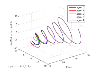
Figure 2: Trajectories of all agents under static network.

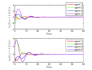
Figure 3: Tracking errors of all agents under static network.

VI-B Switching Network Case

Consider the switching communication graph $\mathcal{\bar{G}}_{\sigma(t)}$, where

$$\begin{split}\sigma(t)=\left\{\begin{array}[]{ll}1,&\hbox{if\ $lT_{0}\leq t<(l+\dfrac{2}{3})T_{0}$}\\ 2,&\hbox{if\ $(l+\dfrac{2}{3})T_{0}\leq t<(l+1)T_{0}$}\\ \end{array}\right.\end{split}$$ (34)

for $l=0,1,2,\cdots$ and $T_{0}=1$, and the two communication graphs are described in Figure 4. It is easy to obtain

$$\begin{split}H_{1}\!=\!\!\left[\!\!\begin{array}[]{cccc}1&0&0&0\\ 0&2&-1&0\\ -1&0&2&-1\\ 0&-1&0&1\\ \end{array}\!\!\right],~{}H_{2}\!=\!\!\left[\!\!\begin{array}[]{cccc}1&0&0&0\\ 0&1&0&0\\ -1&0&1&0\\ 0&-1&-1&2\\ \end{array}\!\!\right].\end{split}$$

Choose $D=I_{4}$. Then it is ready to check that $DH_{1}+H_{1}^{T}D$ and $DH_{2}+H_{2}^{T}D$ are both positive definite. Thus Assumption V.1 is also satisfied.

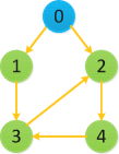
(a) $\bar{\mathcal{G}}_{1}$

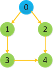
(b) $\bar{\mathcal{G}}_{2}$

Figure 4: Two communication graphs $\bar{\mathcal{G}}_{1}$ and $\bar{\mathcal{G}}_{2}$.

Choosing $\mu_{1}=\mu_{2}=1$, and following the procedures described in Section V, we obtain $\bar{T}=0.0167$ and $K=\left[\begin{array}[]{cc}0.9483&1.3033\\ \end{array}\right]$. We further choose $\underline{T}=0.001$. Then, by Theorem V.1, the distributed sampled-data state feedback control law (3) with $K=\left[\begin{array}[]{cc}0.9483&1.3033\\ \end{array}\right]$ and $T_{s}\in[0.001,0.0167]$ for all $s\in\mathbb{N}$ solves the leader-following consensus problem for the multi-agent system composed of (32) and (33).

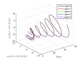
Figure 5: Trajectories of all agents under switching network.

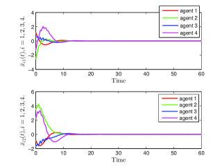
Figure 6: Tracking errors of all agents under switching network.

Simulation is performed with $T_{s}=l_{s}h$, $h=0.001$, $l_{s}$ randomly chosen in the set $\mathcal{S}_{2}=\{1,2,\cdots,16\}$, $s\in\mathbb{N}$, and the same initial states as those for the static network case. The trajectories and tracking errors of all agents under the switching communication graph $\mathcal{\bar{G}}_{\sigma(t)}$ are shown in Figure 5 and Figure 6, respectively. As expected, the trajectories of all follower systems approach the trajectory of the leader system asymptotically, and thus the tracking errors of all agents approach zero asymptotically. Therefore, the leader-following consensus is achieved satisfactorily.

VII Conclusion

In this paper, we have studied the sampled-data leader-following consensus problem for a class of general linear multi-agent systems. Both the static network case and the switching network case have been studied. It has been shown that the problem can be solved by the proposed distributed sampled-data control law if all the sampling intervals are smaller than an explicitly given threshold.

It would be interesting to further consider the sampled-data leader-following consensus problem for linear multi-agent systems with time delay, parameter uncertainties, and to weaken the condition on communication topologies. The results of this paper and some existing results in [8, 23, 28] may shed some light on this future work.

References

- [1] K. J. Astrom, B. Wittenmark, Computer Controlled Systems: Theory and Design, Third Edition, Prentice Hall, Upper Saddle River, NJ, USA, 1997.
- [2] T. Chen and B. A. Francis, Optimal Sampled-Data Control Systems, Springer, London, UK, 1995.
- [3] L. Ding, Q. L. Han and G. Guo, “Network-based leader-following consensus for distributed multi-agent systems,” Automatica, vol. 49, no. 7, pp. 2281-2286, 2013.
- [4] G. F. Franklin, J. D. Powell, M. L. Workman, Digital Control of Dynamic Systems, Third Edition, Addison Wesley Longman, Menlo Park, CA, USA, 1998.
- [5] Y. Gao and L. Wang, “Sampled-data based consensus of cntinuous-time multi-agent systems with time-varying topology,” IEEE Transactions on Automatic Control, vol. 56, no. 5, pp. 1226-1231, 2011.
- [6] X. Ge, Q. L. Han, D. Ding, X. M. Zhang and B. Ning, “A survey on recent advances in distributed sampled-data cooperative control of multi-agent systems,” Neurocomputing, vol. 275, pp. 1684-1701, 2018.
- [7] Z. H. Guan, Z. W. Liu, G. Feng, M. Jian, “Impulsive consensus algorithms for second-order multi-agent networks with sampled information,” Automatica, vol. 48, no. 7, pp. 1397-1404, 2012.
- [8] D. Han, G. Chesi, and Y. S. Hung, “Robust consensus for a class of uncertain multi-agent dynamical systems,” IEEE Transactions on Industrial Informatics, vol. 9, no. 1, pp. 306-312, 2013.
- [9] Y. Hong, G. Chen, and L. Bushnell, “Distributed observers design for leader-following control of multi-agent networks,” Automatica, vol. 44, no. 3, pp. 846-850, 2008.
- [10] R. A. Horn and C. R. Johnson, Topics in Matrix Analysis, New York: Cambridge University Press, 1991.
- [11] J. Hu and Y. Hong, “Leader-following coordination of multi-agent systems with coupling time delays,” Physica A: Statistical Mechanics and its Applications, vol. 374, no. 2, pp. 853-863, 2007.
- [12] A. Jadbabaie, J. Lin, and A. S. Morse, “Coordination of groups of mobile agents using nearest neighbor rules,” IEEE Transactions on Automatic Control, vol. 48, no. 6, pp. 988-1001, 2003.
- [13] V. Kucera, “A contribution to matrix quadratic equations,” IEEE Transactions on Automatic Control, vol. 17, no. 3, pp. 344-347, 1972.
- [14] W. Liu and J. Huang, “Leader-following consensus for linear multi-agent systems via asynchronous sampled-data control,” IEEE Transactions on Automatic Control, DOI: 10.1109/TAC.2019.2948256.
- [15] U. Mnz, A. Papachristodoulou, and F. Allgwer, “Consensus in multi-agent systems with coupling delays and switching topology,” IEEE Transactions on Automatic Control, vol. 56, no. 12, pp. 2976-2982, 2011.
- [16] W. Ni, and D. Cheng, “Leader-following consensus of multi-agent systems under fixed and switching topologies,” Systems & Control Letters, vol. 59, no. 3-4, pp. 209-217, 2010.
- [17] R. Olfati-Saber and R. M. Murray, “Consensus problems in networks of agents with switching topology and time-delays,” IEEE Transactions on Automatic Control, vol. 49, no. 9, pp. 1520-1533, 2004.
- [18] M. J. Park, O. M. Kwon and A. Seuret, “Weighted consensus protocols design based on network centrality for multi-agent systems with sampled-data,” IEEE Transactions on Automatic Control, vol. 62, no. 6, pp. 2916-2922, 2017.
- [19] W. Ren and R. W. Beard, “Consensus seeking in multiagent systems under dynamically changing interaction topologies,” IEEE Transactions on Automatic Control, vol. 50, no. 5, pp. 655-661, 2005.
- [20] Y. Su and J. Huang, “Stability of a class of linear switching systems with applications to two consensus problems,” IEEE Transactions on Automatic Control, vol. 57, no. 6, pp. 1420-1430, 2012.
- [21] Z. J. Tang, T. Z. Huang, J. L. Shao and J. P. Hu, “Leader-following consensus for multi-agent systems via sampled-data control,” IET Control Theory and Applications vol. 5, no. 14, pp. 1658-1665, 2011.
- [22] S. E. Tuna, “LQR-based coupling gain for synchronization of linear systems”, arXiv:0801.3390 [math.OC], 2008.
- [23] F. Xiao and L. Wang, “Asynchronous consensus in continuous-time multi-agent systems with switching topology and time-varying delays,” IEEE Transactions on Automatic Control, vol. 53, no. 8, pp. 1804-1816, 2008.
- [24] D. Xie and Y. Cheng, “Bounded consensus tracking for sampled-data second-order multi-agent systems with fixed and Markovian switching topology,” International Journal of Robust and Nonlinear Control, vol. 25, no. 2, pp. 252-268, 2015.
- [25] G. Xie, H. Liu, L. Wang and Y. Jia, “Consensus in networked multi-agent systems via sampled control: fixed topology case,” 2009 American Control Conference, Hyatt Regency Riverfront, St. Louis, MO, USA, June 10-12, 2009, pp. 3902-3907.
- [26] G. Xie, H. Liu, L. Wang and Y. Jia, “Consensus in networked multi-agent systems via sampled control: switching topology case,” 2009 American Control Conference, Hyatt Regency Riverfront, St. Louis, MO, USA, June 10-12, 2009, pp. 4525-4530.
- [27] W. Yu, W. X. Zheng, G. Chen, W. Ren and J. Cao, “Second-order consensus in multi-agent dynamical systems with sampled position data,” Automatica, vol. 47, no. 7, pp. 1496-1503, 2011.
- [28] L. Zhang, H. Gao, and O. Kaynak, “Network-induced constraints in networked control systems-a survey,” IEEE Transactions on Industrial Informatics, vol. 9, no. 1, pp. 403-416, 2013.
- [29] W. Zhang, Y. Tang, T. Huang, and J. Kurths, “Sampled-data consensus of linear multi-agent systems with packet losses,” IEEE Transactions on Neural Networks and Learning Systems, vol. 28, no. 11, pp. 2516-2517, 2017.
- [30] X. Zhang and J. Zhang, “Sampled-data consensus of general linear multi-agent systems under switching topologies: averaging method,” International Journal of Control, vol. 90, no. 2, pp. 275-288, 2017.
- [31] Y. Zhang and Y. P. Tian “Allowable sampling period for consensus control of multiple general linear dynamical agents in random networks,” International Journal of Control, vol. 83, no. 11, pp. 2368-2377, 2010.