Predicting hydration free energies of the FreeSolv database of druglike molecules with molecular density functional theory

Abstract

We assess the performance of molecular density functional theory (MDFT) to predict hydration free energies of the small drug-like molecules benchmark, FreeSolv. MDFT in the hyper-netted chain approximation (HNC) coupled with a pressure correction predicts experimental hydration free energies of the FreeSolv database within 1 kcal/mol with an average computation time of two cpu.min per molecule. This is the same accuracy as for simulation based free energy calculations that typically require hundreds of cpu.h or tens of gpu.h per molecule.

PASTEUR, Département de chimie, École normale supérieure, PSL University, Sorbonne Université, CNRS, 75005 Paris, France Aqemia, Paris, France

1 Introduction

The ability to predict accurately solvation free energies (SFEs) and solvation profiles unlocks the access to several key thermodynamical quantities of biomolecular systems. SFEs, eventually combined with gas-phase calculations, enable the computation of relative solubilities, binding ¹, ² and transfer³ free energies, partition³ or activity coefficients. The computation of SFEs, i.e. the reversible work to bring a molecule from vacuum to solvent is non-trivial as it requires the sampling of all possible states that can be visited during the transformationIn 2015, considering the difficulty⁴ but nevertheless necessity of evaluating precisely SFEs in the drug design process, important actors of the pharmaceutical industry publicly called the academic world for alternatives, pointing out the lack of precision of current methods⁵.

Multiple approaches for SFE calculations⁴ have been developed since the early 20th century from multiple continuum models⁶, ⁷, ⁸, like COSMO-RS⁹, ¹⁰, ¹¹ or AquaSol¹², exact but resource consuming free energy perturbation approaches with molecular simulations (MD+FEP) to well developed end-point approaches like WaterMap¹³, ¹⁴ or GIST¹⁵.

An alternative to these methods lies within liquid state theories¹⁶. Using liquid state solvation theories like molecular density functional theory¹⁷, ¹⁸, ¹⁹, ²⁰ (MDFT) or 3D-RISM²¹, ²², ²³, ²⁴ , one can predict hydration free energies (HFE) and solvation structures of complex solutes like proteins ²⁵, ²⁰, ²⁶, ²⁷, aluminosilicate surfaces²⁸ or inorganic complexes²⁹. At their heart lies the molecular Ornstein-Zernike equation (MOZ)³⁰, ³¹. In the RISM approach, MOZ loses its molecular nature since molecular correlations are approximated by site-site correlations. The MDFT, on the other hand, keeps the full molecular description of the solvent by solving the full angular-dependent MOZ equation. Since Ding et al. ²⁰, MDFT can be solved efficiently at the hyper-netted chain (HNC) approximation level and predicts SFEs and equilibrium solvent structures in a few minutes which is 3-5 orders of magnitude faster than MD+FEP calculations.

This paper aims at assessing the performance of MDFT-HNC coupled with the recent van der Walls pressure correction³² to predict HFEs of small drug-like molecules of the FreeSolv database³³, ³⁴. The FreeSolv database contains HFEs obtained by experiments and state-of-the-art MD+FEP calculations for 642 small neutral organic molecules. The database has more than 70 chemical functions and molecular masses ranging from 16 to 493 Da. These are typical sizes for drug-like molecules as defined by Lipinski’s ’rule of five’ ³⁵ of molecule’s drug-likeness with a molecular mass criteria maximum at 500 Da. Moreover, 95% of the database has a molecular mass less than 300 Da defined as a limit for lead-like molecules by the ’rule of three’³⁶. The database contains only neutral molecules as measuring SFEs of an isolated charged species requires extra thermodynamic assumptions or introduces other complexities³³ that are still not well understood.

In the first section, we present briefly the MDFT framework and computational details. We refer the reader to refs. ¹⁷, ¹⁸, ¹⁹, ³⁷, ³⁸, ³⁹, ²⁰ for a complete review. In the second section, we evaluate the capacity of MDFT to predict experimental HFEs on the FreeSolv database, compare these results to MD+FEP and 3D-RISM and do an error analysis on selected features of the drug-like molecules in order to be able to infer error bars on the method. Conclusions and perspectives are presented in the third section.

2 Theory

	Full set (619)			Rigid sub-set (520)
	MD+FEP(a)	3D-RISM(b)	MDFTHNC+vdW	MD+FEP	3D-RISM	MDFTHNC+vdW
MAE (kcal/mol)	$1.06\pm 0.08$	$1.11\pm 0.08$	$1.07\pm 0.08$	$0.98\pm 0.07$	$1.04\pm 0.09$	$0.92\pm 0.07$
RMSE (kcal/mol)	$1.41\pm 0.12$	$1.52\pm+0.13$	$1.49\pm 0.13$	$1.29\pm 0.11$	$1.45\pm 0.14$	$1.25\pm 0.11$
ME (kcal/mol)	$-0.37\pm 0.11$	$-0.15\pm 0.12$	$0.07\pm 0.12$	$-0.40\pm 0.11$	$-0.19\pm 0.13$	$-0.07\pm 0.11$
Max err. (kcal/mol)	$7.39$	$7.11$	$8.81$	$4.57$	$7.11$	$4.82$
Pearson’s $R$	$0.94\pm 0.01$	$0.92\pm 0.02$	$0.93\pm 0.01$	$0.94\pm 0.02$	$0.91\pm 0.02$	$0.93\pm 0.01$
Spearman’s $\rho$	$0.94\pm 0.01$	$0.90\pm 0.02$	$0.93\pm 0.02$	$0.94\pm 0.01$	$0.89\pm 0.03$	$0.93\pm 0.02$
Kendall’s $\tau$	$0.80\pm 0.02$	$0.75\pm 0.03$	$0.78\pm 0.02$	$0.79\pm 0.02$	$0.73\pm 0.03$	$0.78\pm 0.03$
cpu.h per solute	$\sim 10^{2}$	$\sim 10^{-1}$	$\sim 10^{-2}$	$\sim 10^{2}$	$\sim 10^{-1}$	$\sim 10^{-2}$

Table 1: Summary of the statistical measures characterizing the correlations between experimental HFEs and those obtained with simulation based free energy techniques, 3D-RISM-KH and MDFT-HNC calculations for the full FreeSolv database and a sub-set of rigid molecules. ME, MAE and RMSE stand for mean, absolute and root-mean-squared error, respectively and Pearson’s $R$ is a linear correlation coefficient and Spearman’s $\rho$ and Kendall’s $\tau$ are monotonic correlation coefficients. All error bars correspond to the 95% confidence interval⁴⁰. (a) Duarte Ramos Matos et al.³³ (b) Roy and Kovalenko ⁴¹.

The molecular density functional theory of classical molecular fluids computes the solvation free energy and equilibrium solvent density around a solute. The solvation free energy of a given solute can be defined as the difference between the grand potential $\Omega$ of the solvated system and the grand potential $\Omega_{\mathrm{bulk}}$ of the bulk solvent. In the classical density functional framework⁴², ⁴³ this difference can be expressed in a functional form:

$$\Delta G_{\textrm{{solv}}}=\Omega-\Omega_{\mathrm{bulk}}=\underset{\rho\rightarrow\rho_{eq}}{\min}\left\{\mathcal{F}[\rho]\right\}=\mathcal{F}[\rho_{\text{eq}}],$$ (1)

where $\mathcal{F}[\rho]$ is a free energy functional to be minimized, $\rho\equiv\rho(\boldsymbol{r},\omega)$ the molecular solvent density, with $\boldsymbol{r}$ a three dimensional vector and $\omega$ the Euler angles $(\theta,\phi,\psi)$, characterizing the position and the orientation of the rigid solvent molecule relative to the rigid solute, and $\rho_{\mathrm{eq}}$ the equilibrium solvent density. In the absence of solute, the equilibrium density is the homogeneous angular and spatial bulk density $\rho_{\textrm{bulk}}\equiv n_{\textrm{bulk}}i/8\pi\text{\texttwosuperior}$ where $n_{\textrm{bulk}}$ is the spatial homogeneous bulk density, typically 0.033 molecule per ų for water at room conditions ($\equiv 1$ kg/L), and $i/8\pi^{2}$ is the angular normalization constant with $i$ the order of the main symmetry axis of the solvent molecule ($i=2$ for water which has a $C_{\mathrm{2v}}$ symmetry with all the integrals of $\psi$ calculated implicitly between 0 and $\pi$).

Without approximations, we split the functional $\mathcal{F}$ into three parts:

$$\mathcal{F}=\mathcal{F}_{{\rm id}}+\mathcal{F}_{{\rm ext}}+\mathcal{F}_{{\rm exc}},$$ (2)

where $\mathcal{F}_{{\rm id}}$ is the ideal term of a fluid of non-interacting particles, $\mathcal{F}_{\textrm{ext}}$ is the external term induced by the solute, and $\mathcal{F}_{{\rm exc}}$ is the excess term that includes structural correlations between solvent molecules.

The ideal term reads

$$\mathcal{F}_{{\rm id}}=k_{{\rm B}}T\int\mathrm{d}\mathbf{r}\mathrm{d}\mathbf{\omega}\left[\rho(\mathbf{r},\mathbf{\omega})\ln\left(\dfrac{\rho(\mathbf{r},\mathbf{\omega})}{\rho_{{\rm bulk}}}\right)-\Delta\rho(\mathbf{r},\mathbf{\omega})\right],$$ (3)

where $k_{{\rm B}}T$ is the thermal energy ($\sim 0.6$ kcal/mol at 300K), $\textrm{d$\boldsymbol{r}$}\equiv\textrm{dxdydz}$, d$\omega\equiv$d$\cos\theta$d$\phi$d$\psi$ and $\Delta\rho(\mathbf{r},\mathbf{\omega})\equiv\rho(\mathbf{r},\mathbf{\omega})-\rho_{{\rm bulk}}$ the excess density over the bulk homogeneous density.

The external contribution comes from the interaction potential $v_{{\rm ext}}$ between the solute molecule and a solvent molecule. It reads

$$\mathcal{F}_{{\rm ext}}=\int\mathrm{d}\mathbf{r}\mathrm{d}\mathbf{\omega}\rho\left(\mathbf{r},\mathbf{\omega}\right)v_{{\rm ext}}\left(\mathbf{r},\mathbf{\omega}\right).$$ (4)

The interaction potential is typically made of a van der Waals term (Lennard-Jones) and electrostatic interactions. Those are the same non-bonded force field parameters as in a molecular dynamics simulation. In what follows, the MDFT computes the SFE for a frozen solute conformer and therefore does not use intramolecular interactions.

The final, excess term describes the excess solvent-solvent contribution. It may be written as a density expansion around the homogeneous bulk density $\rho_{\textrm{bulk}}$:

$$\mathcal{F}_{{\rm exc}}= -\frac{k_{\text{B}}T}{2}\int d\mathbf{r}_{1}\mathrm{d}\mathbf{\omega}_{1}\int d\mathbf{r}_{2}\mathrm{d}\mathbf{\omega}_{2}\Delta\rho\left(\mathbf{r}_{1},\mathbf{\omega}_{1}\right)$$ (5)

$$\hskip 42.67912pt\times c^{(2)}\left(r_{12},\mathbf{\omega}_{1},\mathbf{\omega}_{2}\right)\Delta\rho\left(\mathbf{r}_{2},\mathbf{\omega}_{2}\right)+\mathcal{F}_{{\rm b}}$$

$$= -\frac{k_{\text{B}}T}{2}\int d\mathbf{r}_{1}\mathrm{d}\mathbf{\omega}_{1}\Delta\rho\left(\mathbf{r}_{1},\mathbf{\omega}_{1}\right)\gamma\left(\mathbf{r}_{1},\mathbf{\omega}_{1}\right)+\mathcal{F}_{\textrm{b}}$$

$$= \hskip 2.84544pt\mathcal{F}_{{\rm HNC}}+\mathcal{F}_{{\rm b}},$$

where $c^{(2)}\left(r_{12},\mathbf{\omega}_{1},\mathbf{\omega}_{2}\right)$ is the solvent-solvent molecular direct correlation function of the homogeneous solvent ⁴⁴, ⁴⁵ with $r_{12}$ the distance between $\mathbf{r}_{1}$ and $\mathbf{r}_{2}$. $\mathcal{F}_{\textrm{b}}$ is the bridge functional and $\gamma\equiv c^{(2)}*\Delta\rho$ the indirect solute-solvent correlation defined as the spatial and angular convolution of the excess density with $c^{(2)}$. If one cuts the excess functional expansion at the second order in density, that is, if one cancels the bridge functional⁴⁶, one finds that the MDFT functional produces at its variational minimum the well-known HNC relation for the solute-solvent distribution function:

$$g(\mathbf{r},\omega)=\frac{\rho_{\text{eq}}(\mathbf{r},\omega)}{\rho_{\textrm{bulk}}}=e^{-\beta v_{\textrm{ext}}(\mathbf{r},\omega)+\gamma(\mathbf{r},\omega)},$$ (6)

where $\beta\equiv\frac{1}{k_{B}T}$. Therefore, we call the first term of the excess functional the HNC functional. Higher-order correlation functions of the homogeneous reference fluid can be computed but are not numerically tractable as of today. The rest of the excess term, the so-called bridge functional can be approximated more or less empirically⁴⁷, ⁴⁸, ⁴⁹. However in this paper we benchmark MDFT for small drug-like molecules at its lowest level of accuracy: the MDFT-HNC. There is no bridge functional in what follows.

The algorithms to minimize eq. 5, are described in Ding et al.²⁰. They predict HFEs in few seconds to minutes depending on the supercell size and spacial and angular resolutions. We emphesis the importance of including a pressure correction to the ’raw’ MDFT-HNC results⁵⁰, ⁵¹, ⁵². The following MDFT results include the van der Waals pressure correction described in Robert et al.³² and are referred as MDFT^HNC+vdW results.

2.1 Computational details

MDFT calculations are done with a solute embedded in a cubic supercell of length 21 Å, with periodic boundary conditions, a spatial resolution of 0.33 Å (= 64x64x64 grid nodes) and an angular resolution of 84 orientations per spacial grid node. The MDFT calculations are done on a single frozen configuration of the solute corresponding to the initial configuration given in the FreeSolv database and the solute and solvent molecules are described with the same force field parameters used for the MD+FEP calculations of the FreeSolv database: GAFF force field (v1.7)⁵³ with AM1-BCC partial charges⁵⁴, ⁵⁵ for the solutes and the TIP3P⁵⁶ model for the water. The average computation time is 1 min 53 sec on a single CPU-thread. The MDFT minimization process did not converge for 23 solutes (4% database, see SI for more information). All results we present below are for the 619 molecules that converged.

3 Benchmarking MDFT for small drug-like molecules

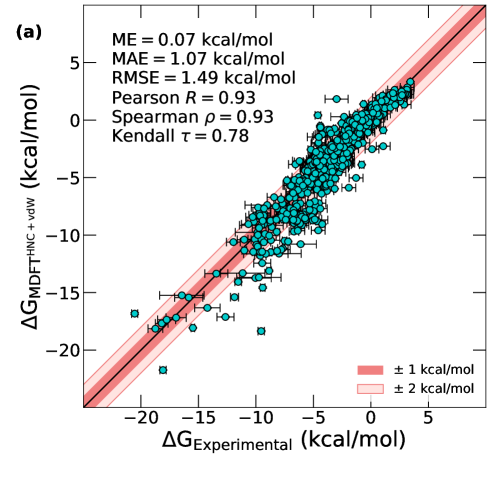
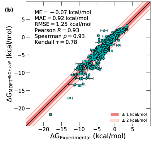
Figure 1: Correlations between hydration free energies predicted by MDFT-HNC with the van der Waals pressure correction and those measured experimentally for (a) the whole FreeSolv database (619 molecules) and (b) a subset of rigid molecules of the FreeSolv database (520 molecules). The subset is defined in the text.

In figure 1a, we show the correlation between experimental HFEs and those obtained with $\mathrm{MDFT^{HNC+vdW}}$. The mean absolute error (MAE) is 1.07 ± 0.08 kcal/mol and the Pearson’s correlation coefficient $R$ is 0.93 ± 0.01. MDFT results also have a small mean (signed) error (ME) of 0.07 ± 0.12 kcal/mol which indicates that MDFT does not have a systematic bias : it is lower in amplitude than the statistical error bars. All the statistical measures characterizing this correlation are summarized in table 1. The error bars on the measures correspond to the 95% confidence interval⁴⁰. Note that as we here are comparing $\mathrm{MDFT^{HNC+vdW}}$, an approached theory, to experimental data, the deviations could be the results of incorrect approximations in $\mathrm{MDFT^{HNC+vdW}}$ or due to bad force field parameterization.

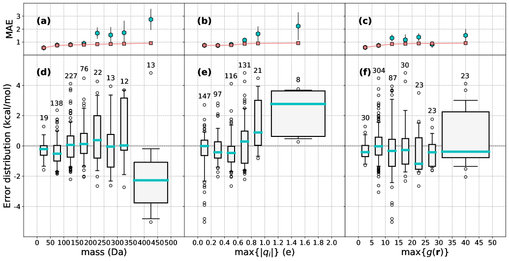
Figure 2: Distribution of mean absolute error between predicted and experimental hydration free energies as a function of three features (a) solute’s molar mass (with bin size of 50 Da), (b) solute’s largest local charge (0.2 e) and (c) the maximum of the 3D $g$ around the solute (5) with turquoise hexagons (error bars correspond to the 95% confidence interval) presenting the MAE of each bin and pink squares the cumulative MAE. The corresponding signed error distributions are presented in d,e and f with turquoise lines corresponding to median error in each bin, the boxes and the whiskers to 25-75% and 5-95% intervals respectively and black circles to fliers outside the 5-95% interval. The numbers above each bin is the population of the bin for the FreeSolv database and for each distribution the last three (350-500 Da), five (1-2 e) or four (30-50) bins are gathered into one in order to be statistically significant.

Table 1 contains also the statistical measures characterizing the correlations between experimental values and those obtained with MD+FEP given by Duarte Ramos Matos et al.³³ and those obtained with 3D-RISM-KH by Roy and Kovalenko⁴¹. Overall the three methods perform at the same accuracy level with similar errors and correlation coefficients. However, MDFT’s computation time is on average less than 2 cpu.min compared to hundreds cpu.h or tens gpu.h with MD+FEP and few tens cpu.min with 3D-RISM⁵⁷, ⁵⁸. Hence for the same accuracy, MDFT has a speedup of 1-2 and 3-4 orders of magnitude when compared to 3D-RISM and MD+FEP respectively. Compared to 3D-RISM, MDFT does not have the consequences from approximating MOZ¹⁶, ⁵⁹, ⁶⁰, ⁶¹.

3.1 Effect of flexibility

Solute flexibility can have an important effect on HFEs⁶², ⁶³, however as mentioned before, the current MDFT calculation is done on a single rigid conformation of the solute, hence the solute flexibility is not taken into account in our MDFT calculation. Therefore, we studied a subset of 520 quasi-rigid solutes to estimate the importance of the lack of solute flexibility in MDFT. We define a solute as rigid if the HFEs obtained with flexible MD+FEP³³ and rigid solute MC+FEP simulations⁶⁴, ³² differ by less than 0.6 kcal/mol which is the average experimental error of the database.

We show the correlation between experimental HFEs and MDFT results for this subset of rigid molecules in figure 1b and the statistical measures characterizing the correlations are summarized in table 1. We observe only a slight improvement of the MAE ($-14\%$) and the RMSE ($-16\%$). However, most of MDFT’s largest outliers can be attributed to the single conformer approximation of the method as the maximum error decreases from 8.81 to 4.82 kcal/mol ($-45\%$) and the number of solutes with absolute errors larger than 3 kcal/mol decrease from 39 to 17 ($-56\%$) when limiting ourselves to rigid solutes.

The following error analyses are done on the subset of 520 rigid solutes.

3.2 Effect of solute’s mass, charges and solvation structure

In order to give an optimal set of requirements and confidence intervals to MDFT-HNC predictions, we now focus on finding sources of errors or correlations between errors. Figure 2 shows the error distribution in function of the solute’s (i) molar mass, (ii) largest partial charge $\mathrm{max}\{|q_{i}|\}$ and (iii) highest value of the 3D solvation structure $\mathrm{max}\{g(\boldsymbol{r})\}$. As shown in figure 2a, the heaviest molecules have the largest deviations to experiment: the MAE increases with the solute’s mass. For solutes with a molar mass larger than 200 Da the MAE is 1.75 kcal/mol, i.e. almost the double than for the whole database. However these molecules present only 12% of the rigid subset so their effect on the total MAE is not significant as seen on the cumulative MAE. Similar trends are present also for the MD+FEP and RISM results with a MAE of 1.78 and 2.21 kcal/mol respectively for these molecules larger than 200 Da (see Figure S1).

Similarly to the molar mass, the deviation to experiment increases with the magnitude of the largest partial charge of the drug-like molecule, positive or negative, (see fig. 2b) with a MAE of 1.84 kcal/mol for solutes with $\mathrm{max}\{|q_{i}|\}>0.8e$ (6% of the rigid subset). The effect is less pronounced for MD+FEP and RISM with MAEs at 1.55 and 1.50 kcal/mol respectively for these molecules (see Figure S1). This is expected for MDFT at the HNC approximation: the second order density expansion of the functional around $\rho=\rho_{\mathrm{bulk}}$, or $g=1$, misses higher order repulsion terms. This leads to problems for cases with densities getting away from $\rho_{\mathrm{bulk}}$: either high densities typically found next to high (partial) charges or large solutes with large volumes where $g=0.$

Besides the solute’s molar mass and partial charges, solute features known a priori, we can also look at the output of a MDFT calculation, that is, the solvation profile, to predict, on this dataset at least, the quality of the MDFT’s HFE predictions. In figure 3, we illustrate the 3D solvent density around 1-amino-4-hydroxy-9,10-anthracenedione (FreeSolv ID: 4371692) with four water-oxygene density isosurfaces ($g=0.5,2.5,5.0$ and $7.5$). Water density maps, that are time consuming to compute using MD⁶⁵ are a direct output of MDFT, again in obtained in 2 min on average. Low densities (fig. 3a) are observed on the limits of the solute’s cavity but also after the first solvation peak (fig. 3d) of the hydroxyl group. The largest oxygen densities (fig. 3d) are observed next to the hydroxyl-hydrogen and the less crowded amine-hydrogen that are potential hydrogen-bond donors.

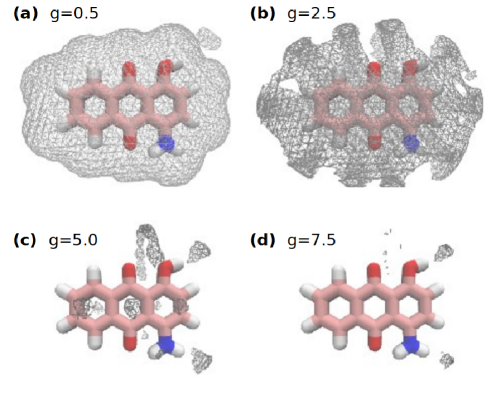
Figure 3: Water density map isosurfaces around 1-amino-4-hydroxy-9,10-anthracenedione at a. $g=0.5$, b. $2.5$, c. $5.0$ and d. $7.5$.

In, figure 2c. we see that the MDFT’s deviation to experiment increases with the maximum height of the solvation peaks with a MAE of 1.24 kcal/mol for solutes with $\mathrm{max}\{g(\boldsymbol{r})\}>20$ (1% of the rigid subset). This result is expected as high density peaks are difficult cases for the HNC approximation as discussed in the previous paragraph. However, the link between the amplitude of the deviation and the solvation structure is less pronounced as for the solute’s mass and partial charges.

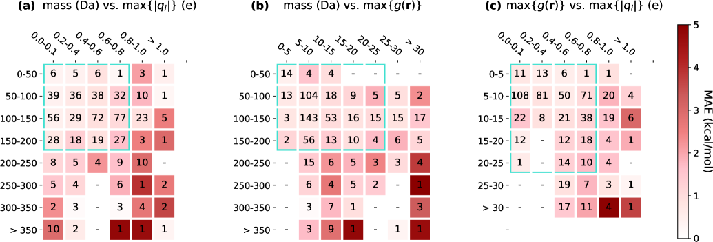
Figure 4: Distribution of mean absolute error between predicted and experimental hydration free energies as a function of two features: a. solute’s mass and largest partial charge, b. solute’s mass and highest solvation peak and c. solute’s highest solvation peak and largest partial charge. The numbers in each bin is the population of the bin.

In figure 4, we show two-dimensional cross distributions of MAE for the three features studied above. Often solutes with high mass and high charges/solvation peaks have the largest deviations but deviations can be large for molecules with only one feature with a ’high’ value (eg. MAE=3.05 kcal/mol for solutes with $\mathrm{max}\{g(\boldsymbol{r})\}=10-15$ and $\mathrm{max}\{|q_{i}|\}>1.0e$ in 4c). The smallest deviations from experiment are found for the solutes with a mass of less than 200 Da, largest partial charge of less than 0.8 and highest solvation peak at less than 25, delimited by the turquoise rectangles in figure 4 (73% of the database), with a MAE at $0.73\pm 0.22$ kcal/mol. A table of the three-dimensional cross distributions of MAE is given in SI.

3.3 Effect of functional groups

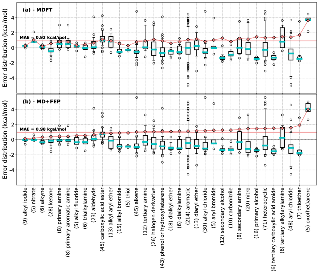
Figure 5: Error distributions of (a) MDFT^HNC+vdW and (b) MD+FEP for the chemical groups with more than 5 solutes present in the database. The number of molecules in each group is written within parenthesis. Turquoise lines correspond to median error in each bin, the boxes and the whiskers to 25-75% and 5-95% intervals respectively and black circles to fliers outside the 5-95% interval. Pink diamonds correspond to the MAE of each functional group and the vertical pink line to total MAE of the rigid subset.

Here we asses the performance of MDFT as a function of the chemical groups present in a solute. In figure 5 we show the error distribution of MDFT^HNC+vdW and reference MD+FEP as a function of each chemical function present in at least five molecules of the database.

We observe a high correlation between the MAEs of MDFT^HNC+vdW and MD+FEP ( $R=0.90$ and $\rho=0.81$). In general functional groups with small/large errors with MD+FEP also have small/large errors with MDFT^HNC+vdW. This indicates that the major part of MDFT’s error comes from the force field parametrization and not the approximated theory itself. This is not unexpected sinci it was shown that MDFT with appropriate partial molar volume corrections reproduce similar SFE’s with an accuracy of $k_{B}T$⁵² or below³². For example it has been noted that the GAFF parametrization of the hydroxyl groups leads to systematic errors in HFEs computed with MD+FEP⁶⁶. Here we observe above average MAEs for primary and secondary alcohols with systematic underestimation of the HFEs (ME < 0 with narrow distribution of errors) for both MD+FEP and MDFT^HNC+vdW.

Nonetheless, there are differences between MDFT’s and MD+FEP’s MAEs: MDFT^HNC+vdW significantly over-performs some groups, like thiols, or under-performs for other groups, like nitrates, when to compared to MD+FEP. Hence the totality of MDFT’s error cannot be attributed to the force field parametrization.

Additionally, we did a similar cross-analysis between chemical functions, as for the mass, partial charge and solvation peak couples. A table of all error bars reconstructed from this analysis is given in SI. To illustrate these error estimates, in figure 6 we show the distribution of MAE for molecules with an aromatic ring, the most frequent chemical function in the database (present in 214 solutes, i.e. 41% of the rigid subset), coupled with another chemical group. We see that in most cases the MAE of an aromatic+another group is close to the overall MAE of the aromatics.

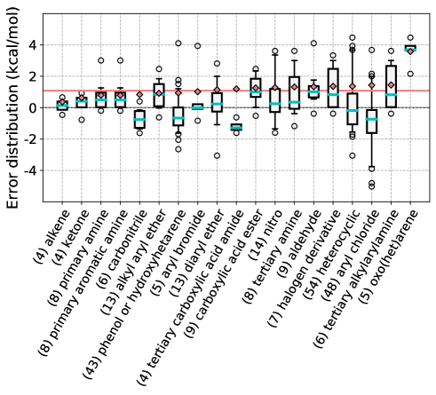
Figure 6: Error distributions of solutes with an aromatic ring coupled to another chemical function for couples present in more than five solutes. The number of molecules in each couple is written within parenthesis. Turquoise lines correspond to median error in each bin, the boxes and the whiskers to 25-75% and 5-95% intervals respectively and black circles to fliers outside the 5-95% interval. Pink diamonds correspond to the MAE of each functional group and the vertical pink line at 1.18 kcal/mol corresponds to the MAE of all the molecules containing an aromatic ring.

Most notably exception is the MAE of aromatic+oxo(het)arene at 3.58 kcal/mol which is much higher than the MAE of all aromatics at 1.08 kcal/mol. This is coherent with oxo(het)arenes having the largest errors of all functional groups. More interesting are the couples like aromatic+alkene (MAE=0.37 kcal/mol) or aromatic+aldehyde (MAE=1.34 kcal/mol) for which the MAEs of the couples are lower or higher than the MAE of the individual chemical functions that they are composed of. Note that these couples contain only 2 and 4 solutes each so these behaviours might be artifacts of limited sampling.

4 Conclusion

Molecular density functional theory in the hyper-netted chain approximation coupled with revised pressure correction predicts experimental hydration free energies with a mean absolute error of 1.07 kcal/mol in 2 minutes on average. Experimental values were available to us during this work but no fitting or adjustments were done to the MDFT method to reproduce the experimental values. Moreover, for rigid solutes MDFT’s accuracy is below 1 kcal/mol. Overall MDFT is at the same level of accuracy as MD+FEP or RISM. MDFT takes on average 2 cpu.min per solute to compute HFE compared to 10+ gpu.h (or 100s cpu.h) by MD+FEP giving a speedup of 3-4 orders of magnitude. As MD+FEP is exact in force field approximation, and as MDFT and MD+FEP have the same accuracy and as the error distributions in function of the chemical functions are similar, the major source of error in MDFT predictions is the force field parameterization.

Looking at the solute’s molar mass, partial charges and the MDFT solvation profile we can estimate the quality of the MDFT HFE prediction. For solutes with a molar mass of less than 200 Da, the largest partial charges at less than 0.8e and highest solvation peak at less than 25, MDFT’s MAE is 0.75 kcal/mol (73% of the database). In this work, we also extracted error bars for {mass, partial charge, solvation peak} triplets and for each kind of chemical function from which we are now able to infer confidence intervals. Additionally, our group is working on coupling MDFT with machine learning approaches to improve MDFT’s accuracy. The error distribution analysis gives information on the types of molecules for which the corrective machine learning coupling will be important and more reference data needs to be produced.

4.1 Acknowledgments

This work has been supported by the Agence Nationale de la Recherche, Project No. ANR BRIDGE AAP CE29.

4.2 Supporting Information Available:

Table S1 : Information on solutes that did not converge with MDFT.
Table S2 : MDFT error bars as a function of the solute’s chemical functions.
Table S3 : MDFT error bars as a function of the solute’s mass, charge and solvation peak.
Figure S1 : Error distributions as a function of the solute’s mass for MD+FEP and 3D-RISM.

References

- Snyder et al. 2011 Snyder, P. W.; Mecinović, J.; Moustakas, D. T.; Thomas, S. W.; Harder, M.; Mack, E. T.; Lockett, M. R.; Heroux, A.; Sherman, W.; Whitesides, G. M. Mechanism of the Hydrophobic Effect in the Biomolecular Recognition of Arylsulfonamides by Carbonic Anhydrase. Proc. Natl. Acad. Sci. U.S.A. 2011, 108, 17889–17894, DOI: 10.1073/pnas.1114107108
- Wang et al. 2011 Wang, L.; Berne, B. J.; Friesner, R. A. Ligand Binding to Protein-Binding Pockets with Wet and Dry Regions. Proc. Natl. Acad. Sci. U.S.A. 2011, 108, 1326–1330, DOI: 10.1073/pnas.1016793108
- Bannan et al. 2016 Bannan, C. C.; Calabró, G.; Kyu, D. Y.; Mobley, D. L. Calculating Partition Coefficients of Small Molecules in Octanol/Water and Cyclohexane/Water. J. Chem. Theory Comput. 2016, 12, 4015–4024, DOI: 10.1021/acs.jctc.6b00449
- Skyner et al. 2015 Skyner, R. E.; McDonagh, J. L.; Groom, C. R.; van Mourik, T.; Mitchell, J. B. O. A Review of Methods for the Calculation of Solution Free Energies and the Modelling of Systems in Solution. Phys. Chem. Chem. Phys. 2015, 17, 6174–6191, DOI: 10.1039/C5CP00288E
- Sherborne et al. 2016 Sherborne, B.; Shanmugasundaram, V.; Cheng, A. C.; Christ, C.; DesJarlais, R. L.; Duca, J. S.; Lewis, R. A.; Loughney, D. A.; Manas, E. S.; McGaughey, G. B.; Peishoff, C. E.; van Vlijmen, H. Collaborating to Improve the Use of Free-Energy and Other Quantitative Methods in Drug Discovery. J. Comput. Aided Mol. Des. 2016, 3, DOI: 10.1007/s10822-016-9996-y
- Tomasi and Persico 1994 Tomasi, J.; Persico, M. Molecular Interactions in Solution: An Overview of Methods Based on Continuous Distributions of the Solvent. Chem. Rev. 1994, 94, 2027–2094, DOI: 10.1021/cr00031a013
- Cramer and Truhlar 1999 Cramer, C. J.; Truhlar, D. G. Implicit Solvation Models Equilibria, Structure, Spectra, and Dynamics. Chem. Rev. 1999, 99, 2161–2200, DOI: 10.1021/cr960149m
- Tomasi et al. 2005 Tomasi, J.; Mennucci, B.; Cammi, R. Quantum Mechanical Continuum Solvation Models. Chem. Rev. 2005, 105, 2999–3094, DOI: 10.1021/cr9904009
- Klamt and Schüürmann 1993 Klamt, A.; Schüürmann, G. COSMO: a New Approach to Dielectric Screening in Solvents with Explicit Expressions for the Screening Energy and Its Gradient. J. Chem. Soc., Perkin Trans. 2 1993, 799–805, DOI: 10.1039/P29930000799
- Klamt 1995 Klamt, A. Conductor-like Screening Model for Real Solvents: A New Approach to the Quantitative Calculation of Solvation Phenomena. J. Phys. Chem. 1995, 99, 2224–2235, DOI: 10.1021/j100007a062
- Klamt 2016 Klamt, A. COSMO-RS for aqueous solvation and interfaces. Fluid Phase Equilib. 2016, 407, 152–158, DOI: 10.1016/j.fluid.2015.05.027
- Koehl and Delarue 2010 Koehl, P.; Delarue, M. AQUASOL: An Efficient Solver for the Dipolar Poisson-Boltzmann-Langevin Equation. J. Chem. Phys. 2010, 132, 064101, DOI: 10.1063/1.3298862
- Young et al. 2007 Young, T.; Abel, R.; Kim, B.; Berne, B. J.; Friesner, R. A. Motifs for Molecular Recognition Exploiting Hydrophobic Enclosure in Protein–Ligand Binding. Proc. Natl. Acad. Sci. U.S.A. 2007, 104, 808–813, DOI: 10.1073/pnas.0610202104
- Abel et al. 2008 Abel, R.; Young, T.; Farid, R.; Berne, B. J.; Friesner, R. A. Role of the Active-Site Solvent in the Thermodynamics of Factor Xa Ligand Binding. J. Am. Chem. Soc. 2008, 130, 2817–2831, DOI: 10.1021/ja0771033
- Nguyen et al. 2012 Nguyen, C. N.; Kurtzman Young, T.; Gilson, M. K. Grid Inhomogeneous Solvation Theory: Hydration Structure and Thermodynamics of the Miniature Receptor Cucurbit[7]uril. J. Chem. Phys. 2012, 137, 044101, DOI: 10.1063/1.4733951
- Hansen and McDonald 2013 Hansen, J.-P.; McDonald, I. R. Theory of Simple Liquids: With Applications to Soft Matter, 4th ed.; Academic Press: Amstersdam, 2013
- Gendre et al. 2009 Gendre, L.; Ramirez, R.; Borgis, D. Classical density functional theory of solvation in molecular solvents: Angular grid implementation. Chem. Phys. Lett. 2009, 474, 366–370, DOI: 10.1016/j.cplett.2009.04.077
- Zhao et al. 2011 Zhao, S.; Ramirez, R.; Vuilleumier, R.; Borgis, D. Molecular density functional theory of solvation: From polar solvents to water. J. Chem. Phys. 2011, 134, 194102, DOI: 10.1063/1.3589142
- Borgis et al. 2012 Borgis, D.; Gendre, L.; Ramirez, R. Molecular Density Functional Theory: Application to Solvation and Electron-Transfer Thermodynamics in Polar Solvents. J. Phys. Chem. B 2012, 116, 2504–2512, DOI: 10.1021/jp210817s
- Ding et al. 2017 Ding, L.; Levesque, M.; Borgis, D.; Belloni, L. Efficient Molecular Density Functional Theory Using Generalized Spherical Harmonics Expansions. J. Chem. Phys. 2017, 147, 094107, DOI: 10.1063/1.4994281
- Hirata and Rossky 1981 Hirata, F.; Rossky, P. J. An Extended RISM Equation for Molecular Polar Fluids. Chem. Phys. Lett. 1981, 83, 329–334, DOI: 10.1016/0009-2614(81)85474-7
- Beglov and Roux 1997 Beglov, D.; Roux, B. An Integral Equation To Describe the Solvation of Polar Molecules in Liquid Water. J. Phys. Chem. B 1997, 101, 7821–7826, DOI: 10.1021/jp971083h
- Kovalenko and Hirata 1998 Kovalenko, A.; Hirata, F. Three-dimensional density profiles of water in contact with a solute of arbitrary shape: a RISM approach. Chem. Phys. Lett. 1998, 290, 237–244, DOI: 10.1016/S0009-2614(98)00471-0
- Kovalenko and Hirata 1999 Kovalenko, A.; Hirata, F. Potential of Mean Force between Two Molecular Ions in a Polar Molecular Solvent: A Study by the Three-Dimensional Reference Interaction Site Model. J. Phys. Chem. B 1999, 103, 7942–7957, DOI: 10.1021/jp991300+
- Imai et al. 2004 Imai, T.; Kovalenko, A.; Hirata, F. Solvation Thermodynamics of Protein Studied by the 3D-RISM Theory. Chem. Phys. Lett. 2004, 395, 1–6, DOI: 10.1016/j.cplett.2004.06.140
- Omelyan and Kovalenko 2015 Omelyan, I.; Kovalenko, A. MTS-MD of Biomolecules Steered with 3D-RISM-KH Mean Solvation Forces Accelerated with Generalized Solvation Force Extrapolation. J. Chem. Theory Comput. 2015, 11, 1875–1895, DOI: 10.1021/ct5010438
- Nguyen et al. 2019 Nguyen, C.; Yamazaki, T.; Kovalenko, A.; Case, D.; Gilson, M.; Kurtzman, T.; Luchko, T. A Molecular Reconstruction Approach to Site-Based 3D-RISM and Comparison to GIST Hydration Thermodynamic Maps in an Enzyme Active Site. PLOS ONE 2019, 14, 1–19, DOI: 10.1371/journal.pone.0219473
- Levesque et al. 2012 Levesque, M.; Marry, V.; Rotenberg, B.; Jeanmairet, G.; Vuilleumier, R.; Borgis, D. Solvation of Complex Surfaces via Molecular Density Functional Theory. J. Chem. Phys. 2012, 137, 224107, DOI: doi:10.1063/1.4769729
- Ruankaew et al. 2019 Ruankaew, N.; Yoshida, N.; Phongphanphanee, S. Solvated lithium ions in defective Prussian blue. IOP Conf. Ser.: Mat. Sci. Eng. 2019, 526, 012032, DOI: 10.1088/1757-899x/526/1/012032
- Blum and Torruella 1972 Blum, L.; Torruella, A. J. Invariant Expansion for Two-Body Correlations: Thermodynamic Functions, Scattering, and the Ornstein-Zernike Equation. J. Chem. Phys. 1972, 56, 303–310, DOI: doi:10.1063/1.1676864
- Blum 1972 Blum, L. Invariant Expansion. II. The Ornstein-Zernike Equation for Nonspherical Molecules and an Extended Solution to the Mean Spherical Model. J. Chem. Phys. 1972, 57, 1862–1869, DOI: doi:10.1063/1.1678503
- Robert et al. 2020 Robert, A.; Luukkonen, S.; Levesque, M. Pressure correction for solvation theories. J. of Chem. Phys. 2020, 152, 191103, DOI: 10.1063/5.0002029
- Duarte Ramos Matos et al. 2017 Duarte Ramos Matos, G.; Kyu, D. Y.; Loeffler, H. H.; Chodera, J. D.; Shirts, M. R.; Mobley, D. L. Approaches for Calculating Solvation Free Energies and Enthalpies Demonstrated with an Update of the FreeSolv Database. J. Chem. Eng. Data 2017, 62, 1559–1569, DOI: 10.1021/acs.jced.7b00104
- Mobley et al. 2009 Mobley, D. L.; Bayly, C. I.; Cooper, M. D.; Shirts, M. R.; Dill, K. A. Small Molecule Hydration Free Energies in Explicit Solvent: An Extensive Test of Fixed-Charge Atomistic Simulations. J. Chem. Theory Comput. 2009, 5, 350–358, DOI: 10.1021/ct800409d
- Lipinski et al. 1997 Lipinski, C. A.; Lombardo, F.; Dominy, B. W.; Feeney, P. J. Experimental and Computational Approaches to Estimate Solubility and Permeability in Drug Discovery and Development Settings. Adv. Drug Deliver. Rev. 1997, 23, 3 – 25, DOI: 10.1016/S0169-409X(96)00423-1
- Congreve et al. 2003 Congreve, M.; Carr, R.; Murray, C.; Jhoti, H. A "Rule of Three" for Fragment-Based Lead Discovery? Drug Discov. Today 2003, 8, 876 – 877, DOI: 10.1016/S1359-6446(03)02831-9
- Ramirez et al. 2002 Ramirez, R.; Gebauer, R.; Mareschal, M.; Borgis, D. Density Functional Theory of Solvation in a Polar Solvent: Extracting the Functional from Homogeneous Solvent Simulations. 2002, 66, 031206–8, DOI: 10.1103/PhysRevE.66.031206
- Jeanmairet et al. 2013 Jeanmairet, G.; Levesque, M.; Vuilleumier, R.; Borgis, D. Molecular Density Functional Theory of Water. J. Phys. Chem. Lett. 2013, 4, 619–624, DOI: 10.1021/jz301956b
- Jeanmairet et al. 2013 Jeanmairet, G.; Levesque, M.; Borgis, D. Molecular Density functional Theory of Water Describing Hydrophobicity at Short and Long Length Scales. J. Chem. Phys. 2013, 139, 154101–1–154101–9, DOI: 10.1063/1.4824737
- 40 For each statistical measure X characterizing a dataset of N points (eg. N=619 for the full set), the measure X’ was computed 10 000 times on N values chosen at random each time from the dataset. The error bars of X correspond to two standard deviations of the X’ distribution.
- Roy and Kovalenko 2019 Roy, D.; Kovalenko, A. Performance of 3D-RISM-KH in Predicting Hydration Free Energy: Effect of Solute Parameters. J. Phys. Chem. A 2019, 123, 4087–4093, DOI: 10.1021/acs.jpca.9b01623
- Mermin 1965 Mermin, N. D. Thermal Properties of the Inhomogeneous Electron Gas. Phys. Rev. 1965, 137, A1441–A1443, DOI: 10.1103/PhysRev.137.A1441
- Evans 1979 Evans, R. The Nature of the Liquid-Vapour Interface and Other Topics in the Statistical Mechanics of Non-Uniform, Classical Fluids. Adv. Phys. 1979, 28, 143, DOI: 10.1080/00018737900101365
- Puibasset and Belloni 2012 Puibasset, J.; Belloni, L. Bridge Function for the Dipolar Fluid from Simulation. 2012, 136, 154503, DOI: doi:10.1063/1.4703899
- Belloni 2017 Belloni, L. Exact Molecular Direct, Cavity, and Bridge Functions in Water System. J. Chem. Phys. 2017, 147, 164121, DOI: 10.1063/1.5001684
- van Leeuwen et al. 1959 van Leeuwen, J.; Groeneveld, J.; de Boer, J. New Method for the Calculation of the Pair Correlation Function. I. Physica 1959, 25, 792 – 808, DOI: 10.1016/0031-8914(59)90004-7
- Levesque et al. 2012 Levesque, M.; Vuilleumier, R.; Borgis, D. Scalar Fundamental Measure Theory for Hard Spheres in Three Dimensions: Application to Hydrophobic Solvation. J. Chem. Phys. 2012, 137, 034115, DOI: 10.1063/1.4734009
- Jeanmairet et al. 2015 Jeanmairet, G.; Levesque, M.; Sergiievskyi, V.; Borgis, D. Molecular Density Functional Theory for Water with Liquid-Gas Coexistence and Correct Pressure. J. Chem. Phys. 2015, 142, 154112, DOI: 10.1063/1.4917485
- Gageat et al. 2017 Gageat, C.; Borgis, D.; Levesque, M. Bridge functional for the molecular density functional theory with consistent pressure and surface tension. 2017, ArXiv:1709.10139
- Sergiievskyi et al. 2014 Sergiievskyi, V.; Jeanmairet, G.; Levesque, M.; Borgis, D. Fast Computation of Solvation Free Energies with Molecular Density Functional Theory: Thermodynamic-Ensemble Partial Molar Volume Corrections. J. Phys. Chem. Lett. 2014, 5, 1935–1942, DOI: 10.1021/jz500428s
- Sergiievskyi et al. 2015 Sergiievskyi, V.; Jeanmairet, G.; Levesque, M.; Borgis, D. Solvation free-energy pressure corrections in the three dimensional reference interaction site model. J. Chem. Phys. 2015, 143, 184116, DOI: 10.1063/1.4935065
- Luukkonen et al. 2020 Luukkonen, S.; Levesque, M.; Belloni, L.; Borgis, D. Hydration free energies and solvation structures with molecular density functional theory in the hyper-netted chain approximation. J. Chem. Phys. 2020, 064110, DOI: 10.1063/1.5142651
- Wang et al. 2004 Wang, J.; Wolf, R. M.; Caldwell, J. W.; Kollman, P. A.; Case, D. A. Development and Testing of a General AMBER Force Field. J. Comput. Chem. 2004, 25, 1157–1174, DOI: 10.1002/jcc.20035
- Jakalian et al. 2000 Jakalian, A.; Bush, B. L.; Jack, D. B.; Bayly, C. I. Fast, Efficient Generation of High-Quality Atomic Charges. AM1-BCC Model: I. Method. J. Comput. Chem. 2000, 21, 132–146, DOI: 10.1002/(SICI)1096-987X(20000130)21:2<132::AID-JCC5>3.0.CO;2-P
- Jakalian et al. 2002 Jakalian, A.; Jack, D. B.; Bayly, C. I. Fast, Efficient Generation of High-Quality Atomic Charges. AM1-BCC Model: II. Parameterization and validation. J. Comput. Chem. 2002, 23, 1623–1641, DOI: 10.1002/jcc.10128
- Jorgensen et al. 1983 Jorgensen, W. L.; Chandrasekhar, J.; Madura, J. D.; Klein, M. L. Comparison of Simple Potential Functions for Simulating Liquid Qater. J. Chem. Phys. 1983, 79, 926–935, DOI: 10.1063/1.445869
- Palmer et al. 2010 Palmer, D. S.; Frolov, A. I.; Ratkova, E. L.; Fedorov, M. V. Towards a Universal Method for Calculating Hydration Free Energies: A 3D Reference Interaction Site Model with Partial Molar Volume Correction. J. Phys. - Condens. Mat. 2010, 22, 492101–1–492101–9, DOI: 10.1088/0953-8984/22/49/492101
- 58 3D-RISM computation time was recovered from a 2010 paper57 as the 2019 paper41 did not discuss computation times.
- Sullivan and Gray 1981 Sullivan, D. E.; Gray, C. Evaluation of Angular Correlation Parameters and the Dielectric Constant in the RISM Approximation. Mol. Phys. 1981, 42, 443–454, DOI: 10.1080/00268978100100381
- Chandler et al. 1978 Chandler, D. et al. General Discussion. Faraday Disc. Chem. Soc. 1978, 66, 71–94, DOI: 10.1039/DC9786600071
- Morriss and Perram 1981 Morriss, G.; Perram, J. Polar hard dumb-bells and a RISM model for water. Molecular Physics 1981, 43, 669–684, DOI: 10.1080/00268978100101591
- Mobley et al. 2008 Mobley, D. L.; Dill, K. A.; Chodera, J. D. Treating Entropy and Conformational Changes in Implicit Solvent Simulations of Small Molecules. J. Phys. Chem. B 2008, 112, 938–946, DOI: 10.1021/jp0764384
- Klimovich and Mobley 2010 Klimovich, P. V.; Mobley, D. L. Predicting Hydration Free Energies Using All-Atom Molecular Dynamics Simulations and Multiple Starting Conformations. J. Comput. Aided Mol. Des. 2010, 24, 307–316, DOI: 10.1007/s10822-010-9343-7
- Belloni 2019 Belloni, L. Non-Equilibrium Hybrid Insertion/Extraction Through the 4th Dimension in Grand-Canonical Simulation. J. Chem. Phys. 2019, 151, 021101, DOI: 10.1063/1.5110478
- Coles et al. 2019 Coles, S. W.; Borgis, D.; Vuilleumier, R.; Rotenberg, B. Computing three-dimensional densities from force densities improves statistical efficiency. J. Chem. Phys. 2019, 151, 064124, DOI: 10.1063/1.5111697
- Fennell et al. 2014 Fennell, C. J.; Wymer, K. L.; Mobley, D. L. A Fixed-Charge Model for Alcohol Polarization in the Condensed Phase, and Its Role in Small Molecule Hydration. J. Phys. Chem. B 2014, 118, 6438–6446, DOI: 10.1021/jp411529h