An Efficient, Practical Algorithm and Implementation for Computing Multiplicatively Weighted Voronoi Diagrams

Abstract

We present a simple wavefront-like approach for computing multiplicatively weighted Voronoi diagrams of points and straight-line segments in the Euclidean plane. If the input sites may be assumed to be randomly weighted points then the use of a so-called overlay arrangement [Har-Peled&Raichel, Discrete Comput. Geom. 53:547–568, 2015] allows to achieve an expected runtime complexity of $\mathcal{O}(n\log^{4}n)$, while still maintaining the simplicity of our approach. We implemented the full algorithm for weighted points as input sites, based on CGAL. The results of an experimental evaluation of our implementation suggest $\mathcal{O}(n\log^{2}n)$ as a practical bound on the runtime. Our algorithm can be extended to handle also additive weights in addition to multiplicative weights, and it yields a truly simple $\mathcal{O}(n\log n)$ solution for solving the one-dimensional version of this problem.

1 Introduction

The mwvd was introduced by Boots [4]. Aurenhammer and Edelsbrunner [2] present a worst-case optimal incremental algorithm for constructing the mwvd of a set of $n$ points in $\mathcal{O}(n^{2})$ time and space. They define spheres on the bisector circles (that are assumed to be situated in the $xy$-plane) and convert them into half-planes in $\mathbb{R}^{3}$ using a spherical inversion. Afterwards, these half-planes are intersected. Thus, every Voronoi region is associated with a polyhedron. Finally, the intersection of every such polyhedron with a sphere that corresponds to the $xy$-plane is inverted back to $\mathbb{R}^{2}$. We are not aware of an implementation of their algorithm, though. (And it seems difficult to implement.) In any case, the linear-time repeated searches for weighted nearest points indicate that its complexity is $\Theta(n^{2})$ even if the combinatorial complexity of the resulting Voronoi diagram is $o(n^{2})$. Later Aurenhammer uses divide&conquer to obtain an $\mathcal{O}(n\log n)$ time and $\mathcal{O}(n)$ space algorithm for the one-dimensional weighted Voronoi diagram [1].

Har-Peled and Raichel [8] show that a bound of $\mathcal{O}(n\log^{2}n)$ holds on the expected combinatorial complexity of a mwvd if all weights are chosen randomly. They sketch how to compute mwvd in expected time $\mathcal{O}(n\log^{3}n)$. Their approach is also difficult to implement because it uses the algorithm by Aurenhammer and Edelsbrunner [2] as a subroutine.

Vyatkina and Barequet [12] present a wavefront-based strategy to compute the mwvd of a set of $n$ lines in the plane in $\mathcal{O}(n^{2}\log n)$ time. The Voronoi nodes are computed based on edge and break-through events. An edge event takes place when an wavefront edge disappears. A break-through event happens whenever a new wavefront edge appears.

Since the pioneering work of Hoff et al. [9] it has been well known that discretized versions of Voronoi diagrams can be computed using the GPU framebuffer. More recently, Bonfiglioli et al. [3] presented a refinement of this rendering-based approach. It is obvious that their approach could also be extended to computing approximate mwvd. However, the output of such an algorithm is just a set of discrete pixels instead of a continuous skeletal structure. Its precision is limited by the resolution of the framebuffer and by the numerical precision of the depth buffer.

2 Our Contribution

Our basic algorithm allows us to compute mwvd in worst-case $\mathcal{O}(n^{2}\log n)$ time and $\mathcal{O}(n^{2})$ space. A refined version makes use of the result by Har-Peled and Raichel [8]: We use their overlay arrangement to keep the expected runtime complexity bounded by $\mathcal{O}(n\log^{4}n)$ if the point sites are weighted randomly. Hence, for the price of a multiplicative factor of $\log n$ we get an algorithm that is easier to implement. Our experiments suggest that this bound is too pessimistic in practice and that one can expect the actual runtime to be bounded by $\mathcal{O}(n\log^{2}n)$. However, our experiments also show that one may get a quadratic runtime if the weights are not chosen randomly. Our algorithm does not require the input sites to have different multiplicative weights, and it can be extended to additive weights and to (disjoint) straight-line segments as input sites. Furthermore, it yields a truly simple $\mathcal{O}(n\log n)$ solution for computing mwvd in one dimension, where all input points lie on a line.

Our implementation is based on exact arithmetic and cgal [11]. It is publicly available on GitHub under https://github.com/cgalab/wevo. To the best of our knowledge, this is the first full implementation of an algorithm for computing mwvd that achieves a decent expected runtime complexity.

3 Preliminaries

Let $S:=\{s_{1},s_{2},\ldots,s_{n}\}$ denote a set of $n$ distinct weighted points in $\mathbb{R}^{2}$ that are indexed such that $w(s_{i})\leq w(s_{j})$ for $1\leq i<j\leq n$, where $w(s_{i})\in\mathbb{R}^{+}$ is the weight associated with $s_{i}$. It is common to regard the weighted distance $d_{w}(p,s_{i})$ from an arbitrary point $p$ in $\mathbb{R}^{2}$ to $s_{i}$ as the standard Euclidean distance $d(p,s_{i})$ from $p$ to $s_{i}$ divided by the weight of $s_{i}$, i.e., $d_{w}(p,s_{i}):=\frac{d(p,s_{i})}{w(s_{i})}$. The (weighted) Voronoi region $\mathcal{VR}_{w}(s_{i},S)$ of $s_{i}$ relative to $S$ is the set of all points of the plane such that no site $s_{j}$ in $S\setminus\{s_{i}\}$ is closer to $p$ than $s_{i}$, that is, $\mathcal{VR}_{w}(s_{i},S):=\left\{p\in\mathbb{R}^{2}:d_{w}(p,s_{i})\leq d_{w}(p,s_{j})\text{~{}for all~{}}j\in\{1,2,\ldots,n\}\right\}$. Then the mwvd, $\mathcal{VD}_{w}(S)$, of $S$ is defined as $\mathcal{VD}_{w}(S):=\bigcup_{s_{i}\in S}\partial\,\mathcal{VR}_{w}(s_{i},S)$.

A connected component of a Voronoi region is called a face. For two distinct sites $s_{i}$ and $s_{j}$ of $S$, the bisector $b_{i,j}$ of $s_{i}$ and $s_{j}$ models the set of points of the plane that are at the same weighted distance from $s_{i}$ and $s_{j}$. Hence, a non-empty intersection of two Voronoi regions is a subset of the bisector of the two defining sites. Following common terminology, a connected component of such a set is called a (Voronoi) edge of $\mathcal{VD}_{w}(S)$. An end-point of an edge is called a (Voronoi) node. It is known that the bisector between two unequally weighted sites forms a circle. An example of a mwvd is shown in Figure 1.

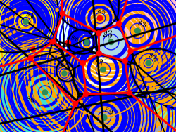
Figure 1: Left: The numbers next to the points indicate their weights and the corresponding mwvd is shown. Right: Wavefronts (in blue) for equally-spaced points in time.

The wavefront $\mathcal{WF}(S,t)$ emanated by $S$ at time $t\geq 0$ is the set of all points $p$ of the plane whose minimal weighted distance from $S$ equals $t$. More formally,

$$\mathcal{WF}(S,t):=\left\{p\in\mathbb{R}^{2}:\min_{s_{i}\in S}d_{w}(p,s_{i})=t\right\}.$$

The wavefront consists of circular arcs which we call wavefront arcs. A common end-point of two consecutive wavefront arcs is called wavefront vertex; see the blue dots in Figure 1.

4 Offset Circles

For the sake of descriptional simplicity, we start with assuming that no point in the plane has the same weighted distance to more than three sites of $S$. For $t\geq 0$, the offset circle $c_{i}(t)$ of the $i$-th site $s_{i}$ is given by a circle centered at $s_{i}$ with radius $t\cdot w(s_{i})$. We find it convenient to regard $c_{i}(t)$ as a function of either time or distance since at time $t$ every point on $c_{i}(t)$ is at Euclidean distance $t\cdot w(s_{i})$ from $s_{i}$, i.e., at weighted distance $t$. We specify a point of $c_{i}(t)$ relative to $s_{i}$ by its polar angle $\alpha$ and its (weighted) polar radius $t$ and denote it by $p_{i}(\alpha,t)$.

For $1\leq i<j\leq n$, consider two sites $s_{i},s_{j}\in S$ and assume that $w(s_{i})\neq w(s_{j})$. Then there exists a unique closed time interval $[t_{ij}^{min},t_{ij}^{max}]$ during which the respective offset circles of $s_{i},s_{j}$ intersect. We say that the two offset circles collide at their mutual collision time $t_{ij}^{min}$, and $s_{j}$ starts to dominate $s_{i}$ at the domination time $t_{ij}^{max}$. For all other times $t$ within this interval the two offset circles $c_{i}(t)$ and $c_{j}(t)$ intersect in two disjoint points $v_{i,j}^{l}(t)$ and $v_{i,j}^{r}(t)$. These (moving) vertices trace out the bisector between $s_{i}$ and $s_{j}$; see Figure 2. Since $v_{i,j}^{l}(t)$ and $v_{i,j}^{r}(t)$ are defined by the same pair of offset circles we refer to $v_{i,j}^{l}(t)$ as the vertex married to $v_{i,j}^{r}(t)$, and vice versa. Every other pair of moving vertices defined by two different pairs of intersecting offset circles is called unmarried. To simplify the notation, we will drop the parameter $t$ if we do not need to refer to a specific time. Similarly, we drop the superscripts $l$ and $r$ if no distinction between married and unmarried vertices is necessary.

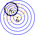
Figure 2: Two married vertices (highlighted by the blue dots) trace out the bisector $b_{ij}$ (in black).

5 A Simple Event-Based Construction Scheme

In this section we describe a simulation of a propagation of the wavefront $\mathcal{WF}(S,t)$ to compute $\mathcal{VD}_{w}(S)$. Since the wavefront is given by a subset of the arcs of the arrangement of all offset circles, one could attempt to study the evolution of all arcs of that arrangement over time. However, it is sufficient to restrict our attention to a subset of arcs of that arrangement. We note that our wavefront can be seen as a kinetic data structure [7].

Clearly, the arc along $c_{i}(t)$ which is inside $c_{j}(t)$ will not belong to $\mathcal{WF}(\{s_{i},s_{j}\},t^{*})$ for any $t^{*}>t$. We will make use of this observation to define inactive and active arcs that are situated along the offset circles.

Definition 5.1 (Active point).

A point $p$ on the offset circle $c_{i}(t)$ is called inactive at time $t$ (relative to $S$) if there exists $j>i$, with $1\leq i<j\leq n$, such that $p$ lies strictly inside of $c_{j}(t)$. Otherwise, $p$ is active (relative to $S$) at time $t$. A vertex $v_{i,j}(t)$ is an active vertex if it is an active point on both $c_{i}(t)$ and $c_{j}(t)$ at time $t$; otherwise, it is an inactive vertex.

Lemma 5.2.

If $p_{i}(\alpha,t)$ is inactive at time $t$ then $p_{i}(\alpha,t^{\prime})$ will be inactive for all times $t^{\prime}\geq t$.

An inactive point $p_{i}(\alpha,t)$ cannot be part of the wavefront $\mathcal{WF}(S,t)$. Lemma 5.2 ensures that none of its future incarnations $p_{i}(\alpha,t^{\prime})$ can become part of the wavefront $\mathcal{WF}(S,t^{\prime})$.

Definition 5.3 (Active arc).

For $1\leq i\leq n$ and $t\geq 0$, an active arc of the offset circle $c_{i}(t)$ at time $t$ is a maximal connected set of points on $c_{i}(t)$ that are active at time $t$. The closure of a maximal connected set of inactive points of $c_{i}(t)$ forms an inactive arc of $c_{i}(t)$ at time $t$.

Every end-point of an active arc of $c_{i}(t)$ is given by the intersection of $c_{i}(t)$ with some other offset circle $c_{j}(t)$, i.e., by a moving vertex $v_{i,j}(t)$. This vertex is active, too.

Definition 5.4 (Arc arrangement).

The aa of $S$ at time $t$, $\mathcal{A}(S,t)$, is the arrangement induced by all active arcs of all offset circles of $S$ at time $t$.

As time $t$ increases, the offset circles expand. This causes the vertices of $\mathcal{A}(S,t)$ to move, but it will also result in topological changes of the arc arrangement.

Definition 5.5 (Collision event).

Let $p_{i}(\alpha,t_{ij}^{min})=p_{j}(\alpha+\pi,t_{ij}^{min})$ be the point of intersection of the offset circles of $s_{i}$ and $s_{j}$ at the collision time $t_{ij}^{min}$, for some fixed angle $\alpha$. A collision event occurs between these two offset circles at time $t_{ij}^{min}$ if the points $p_{i}(\alpha,t)$ and $p_{j}(\alpha+\pi,t)$ have been active for all times $0\leq t\leq t_{ij}^{min}$.

At the time of a collision a new pair of married vertices $v_{i,j}^{l}(t)$ and $v_{i,j}^{r}(t)$ is created. Of course, we have $v_{i,j}^{l}(t_{ij}^{min})=v_{i,j}^{r}(t_{ij}^{min})=p_{i}(\alpha,t_{ij}^{min})$.

Definition 5.6 (Domination event).

Let $p_{i}(\alpha,t_{ij}^{max})=p_{j}(\alpha,t_{ij}^{max})$ be the point of intersection of the offset circles of $s_{i}$ and $s_{j}$ at the domination time $t_{ij}^{max}$, for some fixed angle $\alpha$. A domination event occurs between these two offset circles at time $t_{ij}^{max}$ if the points $p_{i}(\alpha,t)$ and $p_{j}(\alpha,t)$ have been active for all times $0\leq t\leq t_{ij}^{max}$.

At the time of a domination event the married vertices $v_{i,j}^{l}(t_{ij}^{max})$ and $v_{i,j}^{r}(t_{ij}^{max})$ coincide and are removed.

Definition 5.7 (Arc event).

An arc event $e$ occurs at time $t_{e}$ when an active arc $a_{i}$ shrinks to zero length because two unmarried vertices $v_{i,j}(t_{e})$ and $v_{i,k}(t_{e})$ meet in a point $p_{e}$ on $c_{i}(t_{e})$.

Lemma 5.2 implies that $p_{i}(\alpha,t)$ has been active for all times $t\leq t_{e}$ if $p_{i}(\alpha,t_{e})=p_{e}$. At the time of an arc event two unmarried vertices trade their places along an offset circle. Now suppose that the two unmarried vertices $v_{i,j}(t_{e})$ and $v_{i,k}(t_{e})$ meet in a point $p_{e}$ along $c_{i}(t_{e})$ at the time $t_{e}$ of an arc event, thereby causing an active arc of $c_{i}(t_{e})$ to shrink to zero length. Hence, the offset circles of $s_{i},s_{j}$ and $s_{k}$ intersect at the point $p_{e}$ at time $t_{e}$. If $c_{j}(t)$ and $c_{k}(t)$ did not intersect for $t<t_{e}$ then we also get a collision event between $c_{j}(t)$ and $c_{k}(t)$ at time $t_{e}$, see Figure 3(a). (This configuration can occur for any relative order of the weights $w(s_{i}),w(s_{j}),w(s_{k})$.) Otherwise, one or both of the married vertices $v_{j,k}^{l}(t_{e})$ and $v_{j,k}^{r}(t_{e})$ must also coincide with $p_{e}$. If both coincide with $p_{e}$ then we also get a domination event between $c_{j}(t)$ and $c_{k}(t)$ at time $t_{e}$ and we have $w(s_{j})<w(s_{k})$, see Figure 3(b). The scenarios remaining for the case that only one of $v_{j,k}^{l}(t_{e})$ and $v_{j,k}^{r}(t_{e})$ coincides with $p_{e}$ are detailed in the following lemma.

(a)

(b)

Figure 3: (a) The configuration shortly before (left) and after (right) a collision event as well as an arc event occur simultaneously at the same point $p_{e}$. In the left figure the offset arcs at the time of the event are shown in gray. Arcs and vertices that are on $\mathcal{WF}(\{s_{i},s_{j},s_{k}\},t)$ are highlighted in blue. Other active arcs and vertices are depicted by solid orange lines and filled disks, while inactive arcs and vertices are depicted by dashed orange lines and circles. (b) The configuration shortly before and after a domination event and an arc event occur simultaneously at the same point $p_{e}$.

Lemma 5.8.

Let $i<j<k$ and consider an arc event such that exactly the three vertices $v_{i,j}(t_{e})$, $v_{i,k}(t_{e})$, and $v_{j,k}(t_{e})$ coincide at time $t_{e}$. Then either

• all three vertices were active before the event, see fig. 4(a), or

• $v_{i,j}$ and $v_{j,k}$ were active and $v_{i,k}$ was inactive before the event, see fig. 4(b), or

• $v_{i,k}$ and $v_{j,k}$ were active and $v_{i,j}$ was inactive before the event, see fig. 4(c).

(a) The two possible configurations shortly before (shown in the left figures) and after (shown in the right figures) one active arc disappears on $c_{i}(t)$ if no collision or domination event occurs at the same point. We get the collapse of all three arcs of an active-arc triangle.

(b) The two possible configurations shortly before (left) and after (right) one active arc disappears on $c_{j}(t)$ and another active arc appears on $c_{k}(t)$.

(c) The two possible configurations shortly before (left) and after (right) one active arc disappears on $c_{k}(t)$ and another active arc appears on $c_{j}(t)$.

Figure 4: The six different configurations that can occur for arc events for $1\leq i<j<k\leq n$.

We now describe an event-handling scheme that allows us to trace out $\mathcal{VD}_{w}(S)$ by simulating the expansion of the arcs of $\mathcal{A}(S,t)$ as $t$ increases, see Figure 5. We refer to this process as arc expansion.

For each site we maintain a search data structure to keep track of all active arcs during the arc expansion. This active offset $o_{i}$ of $s_{i}$ holds the set of all arcs of $c_{i}(t)$ which are active at time $t$ sorted in counter-clockwise angular order around $s_{i}$, and supports the following basic operations in time logarithmic in the number of arcs stored:

• It supports the insertion and deletion of active arcs as well as the lookup of their corresponding vertices.

• It supports point-location queries, allowing us to identify that active arc within $o_{i}$ which contains a query point $p$ on $c_{i}(t)$.

Every active offset contains at most $2(n-1)$ vertices and, thus, $O(n)$ active arcs. Hence, each such operation on an active offset takes $\mathcal{O}(\log n)$ time in the worst case.

Figure 5: A snapshot of the arc expansion for the input shown in Figure 1. Active arcs that are currently not part of the wavefront are drawn in orange.

Checking and handling the configurations shown in Figures 3(a) to 4 can be done by using only basic operations within the respective active offsets. The events themselves are stored in a priority queue $\mathcal{Q}$ ordered by the time of their occurrence. If two events take place simultaneously at the same point then collision events are prioritized higher than arc events, and arc events have to be handled before domination events. Four auxiliary operations are utilized that allow a more compact description of this process. Each one takes $\mathcal{O}(\log n)$ time.

• The collapse-operation takes place from $v_{i,x}$ to $v_{j,k}$ within an active offset $o_{x}$, with $x\in\{j,k\}$, in which $v_{i,x}$ and $v_{j,k}$ bound an active arc $a_{x}$ that is already part of $o_{x}$; see Figure 6(a). It determines the neighboring active arc $a_{x}^{\prime}$ of $a_{x}$ that is bounded (on one side) by $v_{i,x}$, deletes $a_{x}$ from $o_{x}$, and replaces $v_{i,x}$ by $v_{j,k}$ in $a_{x}^{\prime}$.

• The counterpart of the collapse-operation is the expand-operation; see Figure 6(b). It happens from $v_{j,k}$ to $v_{i,x}$ in which $v_{j,k}$ bounds an active arc $a_{x}^{\prime}$ within $o_{x}$. The expansion will either move along a currently inactive or an already active portion of the offset circle of $s_{x}$. In the latter case, $v_{j,k}$ is replaced by $v_{i,x}$ in $a_{x}^{\prime}$. In any case, we insert the respective active arc that is bounded by $v_{i,x}$ and $v_{j,k}$ into $o_{x}$.

• A split-operation involves two active offsets $o_{i}$ and $o_{j}$ as well as a point $p_{e}$ which is situated within the active arcs $a_{i}:=(v_{i,s},v_{i,e})$ and $a_{j}:=(v_{j,s^{\prime}},v_{j,e^{\prime}})$ within $o_{i}$ and $o_{j}$, respectively; see Figure 7(a). Two married vertices $v_{i,j}^{l}$ and $v_{i,j}^{r}$ are created. Afterwards $a_{i}$ and $a_{j}$ are removed from $o_{i}$ and $o_{j}$, respectively. Two new active arcs $(v_{i,s},v_{i,j}^{l})$ and $(v_{i,j}^{r},v_{i,e})$ are created and inserted into $o_{i}$. Furthermore, the three active arcs $(v_{j,e},v_{i,j}^{r})$, $(v_{i,j}^{r},v_{i,j}^{l})$, and $(v_{i,j}^{l},v_{j,e})$ are inserted into $o_{j}$. If $a_{i}$ and $a_{j}$ were wavefront arcs then the newly created married vertices coincide with wavefront vertices and the newly inserted active arcs except $(v_{i,j}^{r},v_{i,j}^{l})$ are marked as wavefront arcs.

• During a merge-operation, exactly two offset circles interact; see Figure 7(b). The active arcs $a_{i}$ and $a_{j}$ bounded by the two corresponding married vertices $v_{i,j}^{r}$ and $v_{i,j}^{l}$ are removed from $o_{i}$ and $o_{j}$, respectively. Additionally, the active arcs $(v_{j,s},v_{i,j}^{r})$ and $(v_{i,j}^{l},v_{j,e})$ that were adjacent to $a_{j}$ within $o_{j}$ are removed. Finally, a new active arc $a_{j}^{\prime}:=(v_{j,s},v_{j,e})$ is inserted into $o_{j}$. If $a_{j}$ was a wavefront arc then $a_{j}^{\prime}$ is also marked as a wavefront arc.

(a)

(b)

Figure 6: (a) A collapse-operation from $v_{i,k}$ to $v_{j,k}$ takes place within $o_{k}$. (b) An expand-operation happens within $o_{j}$ from $v_{j,k}$ to $v_{i,j}$.

(a)

(b)

Figure 7: (a) A split-operation happens when at the time of a collision event. (b) A merge-operation happens at the time of a domination event.

Domination events and arc events are easy to detect. The point and time of a collision is trivial to compute for any pair of offset circles, too. Unfortunately there is no obvious way to identify those pairs of circles for which this intersection will happen within portions of these offset circles which will still be active at the time of the collision. Hence, for the rest of this section we assume that all collisions among all pairs of offset circles are computed prior to the actual arc expansion. Lemma 5.9 verifies that our algorithm correctly simulates the arc expansion.

Lemma 5.9.

For time $t>0$, the arc arrangement $\mathcal{A}(S,t)$ can be obtained from $\mathcal{A}(S,0)$ by modifying it according to all collision events, domination events and arc events that occur till time $t$, in the order in which they appear.

If the maximum weight of all sites is associated with only one site then there will be a time $t$ when the offset circle of this site dominates all other offset circles, i.e., when $\mathcal{WF}(S,t)$ contains only this offset circle as one active arc. Obviously, at this time no further event can occur and the arc expansion stops. If multiple sites have the same maximum weight then $\mathcal{Q}$ can only be empty once $\mathcal{WF}(S,t)$ contains only one loop of active arcs which all lie on offset circles of these sites and if all wavefront vertices move along rays to infinity.

Lemma 5.10.

An active arc or active vertex within an active offset is identified and marked as a wavefront arc (wavefront vertex, resp.) at time $t\geq 0$ if and only if it lies on $\mathcal{WF}(S,t)$.

If we allow points in $\mathbb{R}^{2}$ to have the same weighted distance to more than three sites then we need to modify our strategy. In particular, we need to take care of constellations in which more than three arc events happen simultaneously at the same point. In such a case it is necessary to carefully choose the sequence in which the corresponding arc events are handled. More precisely, an arc event may only be handled (without corrupting the state of the active offsets) whenever the respective active vertices are considered neighboring within the active offsets. If the active vertices that participate in an arc event are not currently neighboring then we can always find an arc event whose active vertices are neighboring that happens simultaneously at the same location by walking along the corresponding active offsets. By dealing with the arc events in this specific order, we generate multiple coinciding Voronoi nodes of degree three. Domination events that occur simultaneously at the same point $p_{e}$ are processed in increasing order of the weights. Note that this order can already be established at the time when an event is inserted into $\mathcal{Q}$, at no additional computational cost. Simultaneous multiple collision events at the same point $p_{e}$ either involve arcs that are not active or coincide with arc events. These arc events automatically establish a sorted order of the active arcs around $p_{e}$, thus allowing us to avoid an explicit (and time-consuming) sorting.

Lemma 5.11.

During the arc expansion $\mathcal{O}(n^{2})$ collision and domination events are computed.

We know that collision events create and domination events remove active vertices (and make them inactive for good). A collapse of an entire active-arc triangle causes two vertices to become inactive. During every other arc event at least one active vertex becomes inactive, but at the same time one inactive vertex may become active again. In order to bound the number of arc events it is essential to determine how many vertices can be active and how often a vertex can undergo a reactivation, i.e., change its status from inactive to active. (Note that Lemma 5.2 is not applicable to a moving vertex since its polar angle does not stay constant.) We now argue that the total number of reactivations of inactive vertices is bounded by the number of different vertices that ever were active during the arc expansion.

Lemma 5.12.

Every reactivation of a moving vertex during an arc event forces another moving vertex to become inactive and remain inactive for the rest of the arc expansion.

Lemma 5.13.

Let $h$ be the number of different vertices that ever were active during the arc expansion. Then $\mathcal{O}(h)$ arc events can take place during the arc expansion.

Theorem 5.14.

The multiplicatively weighted Voronoi diagram $\mathcal{VD}_{w}(S)$ of a set $S$ of $n$ weighted point sites can be computed in $\mathcal{O}(n^{2}\log n)$ time and $\mathcal{O}(n^{2})$ space.

Additionally, in the appendix we argue that the one-dimensional mwvd can be computed efficiently using a wavefront-based strategy.

Theorem 5.15.

The multiplicatively weighted Voronoi diagram $\mathcal{VD}_{w}(S)$ of a set $S$ of $n$ weighted point sites in one dimension can be computed in $\mathcal{O}(n\log n)$ time and $\mathcal{O}(n)$ space.

6 Reducing the Number of Collisions Computed

Experiments quickly indicate that the vast majority of pairwise collisions computed a priori never ends up on pairs of active arcs. Furthermore, the resulting Voronoi diagrams show a quadratic combinatorial complexity only for contrived input data. We make use of the following results to determine all collision events in near-linear expected time. Throughout this section, we assume that for each site $s_{i}\in S$ the corresponding weight $w(s_{i})$ is independently sampled from some probability distribution.

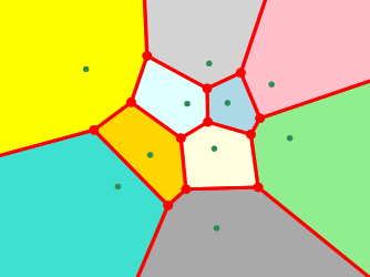
Figure 8: The overlay arrangement is generated by inserting the sites ordered by decreasing weights.

Definition 6.1 (Candidate Set).

Consider an arbitrary (but fixed) point $q\in\mathbb{R}^{2}$, and let $s$ be its nearest neighbor in $S$ under the weighted distance. Let $s^{\prime}\in S\setminus\{s\}$ be another site. Since $s$ is the nearest neighbor of $q$ we know that either $s$ has a higher weight than $s^{\prime}$ or a smaller Euclidean distance to $q$ than $s^{\prime}$. Thus, one can define a candidate set for a weighted nearest neighbor of $q$ which consists of all sites $s\in S$ such that all other sites in $S$ either have a smaller weight or a larger Euclidean distance to $q$.

Lemma 6.2 (Har-Peled and Raichel [8]).

For all points $q\in\mathbb{R}^{2}$, the candidate set for $q$ among $S$ is of size $\mathcal{O}(\log n)$ with high probability.

Lemma 6.3 (Har-Peled and Raichel [8]).

Let $K_{i}$ denote the Voronoi cell of $s_{i}$ in the unweighted Voronoi diagram of the $i$-th suffix $S_{i}:=\{s_{i},\ldots,s_{n}\}$. Let $\mathcal{O}\mathcal{A}$ denote the arrangement formed by the overlay of the regions $K_{1},\ldots,K_{n}$. Then, for every face $f$ of $\mathcal{O}\mathcal{A}$, the candidate set is the same for all points in $f$.

Figure 8 shows a sample overlay arrangement. Kaplan et al. [10] prove that this overlay arrangement has an expected complexity of $\mathcal{O}(n\log n)$. Note that their result is applicable since inserting the points in sorted order of their randomly chosen weights corresponds to a randomized insertion. These results allow us to derive better complexity bounds.

Theorem 6.4 (Kaplan et al. [10]).

The expected combinatorial complexity of the overlay of the minimization diagrams that arises during a randomized incremental construction of the lower envelope of $n$ hyperplanes in $\mathbb{R}^{d}$, for $d\geq 2$, is $\mathcal{O}(n^{\lfloor d/2\rfloor})$, for $d$ even, and $O(n^{\lfloor d/2\rfloor}\log n)$, for $d$ odd. The bounds for $d$ even and for $d=3$ are tight in the worst case.

Lemma 6.5.

If a collision event occurs between the offset circles of two sites $s_{i},s_{j}\in S$ then there exists at least one candidate set which includes both $s_{i}$ and $s_{j}$.

Theorem 6.6.

All collision events can be determined in $\mathcal{O}(n\log^{3}n)$ expected time by computing the overlay arrangement $\mathcal{O}\mathcal{A}$ of a set $S$ of $n$ input sites.

Thus, the number $h$ of vertices created during the arc expansion can be expected to be bounded by $\mathcal{O}(n\log^{3}n)$. Lemma 5.13 tells us that the number of arc events is in $\mathcal{O}(h)$. Therefore, $\mathcal{O}(n\log^{3}n)$ events happen in total.

Theorem 6.7.

A wavefront-based approach allows to compute the multiplicatively weighted Voronoi diagram $\mathcal{VD}_{w}(S)$ of a set $S$ of $n$ (randomly) weighted point sites in expected $\mathcal{O}(n\log^{4}n)$ time and expected $\mathcal{O}(n\log^{3}n)$ space.

7 Extensions

Consider a set $S^{\prime}$ of $n$ disjoint weighted straight-line segments in $\mathbb{R}^{2}$. A wavefront propagation among weighted line segments requires us to refine our notion of “collision”. We call an intersection of two offset circles a non-piercing collision event if it marks the initial contact of the two offset circles. That is, it occurs when the first pair of moving vertices appear. We call an intersection of two offset circles a piercing collision event if it takes place when two already intersecting offset circles intersect in a third point for the first time; see Figure 9. In this case, a second pair of moving vertices appear.

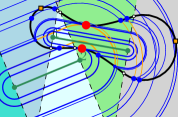
Figure 9: An example of a non-piercing (left) as well as a piercing collision event (right).

Hence, a minor modification of our event-based construction scheme is sufficient to extend it to weighted straight-line segments; see Figure 10. We only need to check whether a piercing collision event that happens at a point $p_{e}$ at time $t_{e}$ currently is part of $\mathcal{WF}(S^{\prime},t_{e})$. In such a case the two new vertices as well as the corresponding active arc between them need to be flagged as part of $\mathcal{WF}(S^{\prime},t_{e})$.

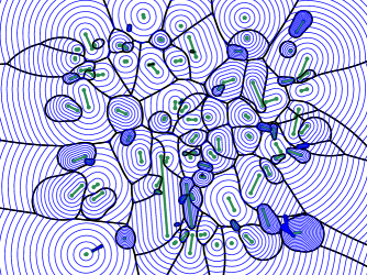
Figure 10: The mwvd of a set of weighted points and weighted straight-line segments together with a family of wavefronts for equally-spaced points in time.

An extension to additive weights can be integrated easily into our scheme by simply giving every offset circle a head-start of $w_{a}(s_{i})$ at time $t=0$, where $w_{a}(s_{i})\geq 0$ denotes the real-valued additive weight that is associated with $s_{i}$.

8 Experimental Evaluation

We implemented our full algorithm for multiplicatively weighted points as input sites, based on cgal and exact arithmetic. In particular, we use cgal’s Arrangement_2 package for computing the overlay arrangement and its Voronoi_diagram_2 package for computing unweighted Voronoi diagrams. The computation of the mwvd itself utilizes cgal’s Exact_circular_kernel_2 package which is based on the Gmpq number type. The obvious advantage of using exact number types is that events are guaranteed to be processed in the right order even if they occur nearly simultaneously at nearly the same place. One of the main drawbacks of exact number types is their memory consumption which is significantly (and sometimes unpredictably) higher than when standard floating-point numbers are used.

We used our implementation for an experimental evaluation and ran our code on over $8000$ inputs ranging from $256$ vertices to $500\,000$ vertices. For all inputs all weights were chosen uniformly at random from the interval $[0,1]$. All tests were carried out with cgal 5.0 on an Intel Core i9-7900X processor clocked at $3.3\text{\,}\mathrm{GHz}$.

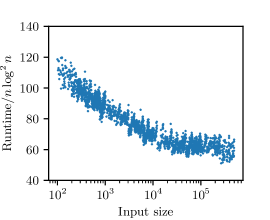
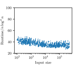
(a) Left: The overall runtime results for inputs with randomly generated weights and point coordinates. Right: The runtime consumed by the computation of the corresponding overlay arrangements. All runtimes were divided by $n\log^{2}n$.

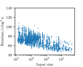
(b) The overall runtime results for inputs with randomly generated weights and vertices of real-world polygons and polygons of the Salzburg database of polygonal data [5, 6] taken as input points. The runtimes were divided by $n\log^{2}n$.

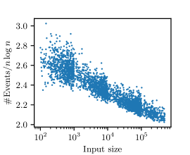
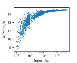
(c) The left plot shows the total number of (valid and invalid) collision events (divided by $n\log n$); the right plot shows the number of arc events (divided by $n$) processed during the arc expansion. All point coordinates and weights were generated randomly.

Figure 11: Experimental evaluation.

In any case, the number of events is smaller than predicted by the theoretical analysis. This is also reflected by our runtime statistics: In Figures 11(a) and 11(b) the runtime that was consumed by the computation of a mwvd is plotted. We ran our tests on two different input classes: The point locations were either generated randomly, i.e., they were chosen according to either a uniform or a normal distribution, or obtained by taking the vertices of real-world polygons or polygons of the brand-new Salzburg database of polygonal data [5, 6]. Summarizing, our tests suggest an overall runtime of $\mathcal{O}(n\log^{2}n)$ for both input classes. In particular, the actual geometric distribution of the sites does not have a significant impact on the runtime if the weights are chosen randomly: For real-world, irregularly distributed sites the runtimes are scattered more wildly than in the case of uniformly distributed sites, but they do not increase. The numbers of collision events and arc events that occurred during the arc expansion are plotted in Figure 11(c). Our tests suggest that we can expect to see at most $3n\log n$ collision events and at most most $14n$ arc events to occur. Note that the number of arc events forms an upper bound on the number of Voronoi nodes of the final mwvd. That is, random weights seem to result in a linear combinatorial complexity of the mwvd.

It is natural to ask how much these results depend on the randomness of the weights. To probe this question we set up a second series of experiments: We sampled points uniformly within a square with side-length $\sqrt{2}$ and then tested different weights. Let $d(s)$ be the distance of the site $s\in S$ from the center of the square, and let $r(s)$ be a number uniformly distributed within the interval $[0,1]$. Of course, $0\leq d(s)\leq 1$. Then we assign $\nicefrac{{\alpha\cdot d(s)+\beta\cdot r(s)}}{{(\alpha+\beta)}}$ as weight to $s$, with $\alpha$ and $\beta$ being the same arbitrary but fixed non-negative numbers for all sites of $S$. Figure 12 shows the results obtained for the same sets of points and the $(\alpha,\beta)$-pairs $(1,0)$, $(9,1)$, $(7,3)$, $(1,1)$ and $(0,1)$. This test makes it evident that the bounds on the complexities need not hold if the weights are not chosen randomly, even for a uniform distribution of the sites. Rather, this may lead to a linear number of candidates per candidate set and a quadratic runtime complexity, as shown in Figure 12.

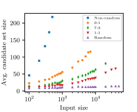
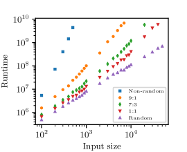
Figure 12: The plots show how the average number of candidates (left) and the total runtime (right) depend on the weights assigned to the sites. Each marker on the $x$-axes indicates the number $n$ of input sites uniformly distributed within a square.

9 Conclusion

We present a wavefront-like approach for computing the mwvd of points and straight-line segments. Results by Kaplan et al. [10] and Har-Peled and Raichel [8] allow to predict an $\mathcal{O}(n\log^{4}n)$ expected time complexity for point sites with random weights. We also discuss a robust, practical implementation which is based on cgal and exact arithmetic. Extensive tests of our code indicate an average runtime of $\mathcal{O}(n\log^{2}n)$ if the sites are weighted randomly. To the best of our knowledge, there does not exist any other code for computing mwvd that is comparatively fast. A simple modification of our arc expansion scheme makes it possible to handle both additive and multiplicative weights simultaneously. Our code is publicly available on GitHub under https://github.com/cgalab/wevo. Figure 13 shows several examples of mwvd computed by our implementation.

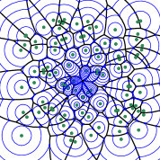
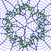
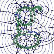
Figure 13: Several examples of mwvd are shown in the top figures. The bottom figures illustrate a series of uniformly distributed wavefronts that have been derived from the corresponding mwvd.

Appendix A Algorithm

Data: A set $S$ of disjoint weighted input sites that are in general position.

Result: A doubly-connected edge list $\mathcal{D}$ that holds $\mathcal{VD}_{w}(S)$.

1 Compute all collision events for every pair of sites in $S$ and insert them into the priority queue $\mathcal{Q}$;

2 Insert an active arc that is bounded by two dummy vertices into each active offset that marks the respective offset circle as entirely active;

3 Mark all offset circles as being part of the wavefront;

4 while $\mathcal{Q}$ is not empty do

5       Pop the next event $e$ from $\mathcal{Q}$ that occurs at time $t_{e}>0$ at the point $p_{e}\in\mathbb{R}^{2}$;

6       if $e$ is a collision event then

7             Determine the two offset circles $c_{i}(t_{e})$ and $c_{j}(t_{e})$ that collide;

8             if $p_{e}$ is situated within active arcs $a_{i}$ and $a_{j}$ of $o_{i}$ and $o_{j}$ then

9                   Split $a_{i}$ and $a_{j}$ at $p_{e}$;

10                   if $a_{i}$ and $a_{j}$ are wavefront arcs then

11                         Add a new degree-two node $v$ to $\mathcal{D}$ as well as the corresponding half-edges that start at $v$.

12                  

13            

14       else if $e$ is a domination event then

15             Determine $c_{j}(t_{e})$ that dominates $c_{i}(t_{e})$;

16             if $p_{e}$ is situated within active arcs $a_{i}$ and $a_{j}$ of $o_{i}$ and $o_{j}$ then

17                   Merge the two newly neighboring active arcs within $o_{j}$;

18                   if $a_{i}$ is a wavefront arc then

19                         Add a new degree-two node $v$ to $\mathcal{D}$ and link the corresponding half-edges to $v$.

20                  

21            

22       else

            // $e$ is an arc event.

23             Determine the three vertices $v_{i,j}$, $v_{i,k}$, and $v_{j,k}$ that participate in $e$;

24             if $v_{i,j}$, $v_{i,k}$, and $v_{j,k}$ are all active then

25                   Extract the other two arc events from $\mathcal{Q}$ which indicate the disappearances of the remaining two active that form the active-arc triangle;

26                   Determine the active arcs $a_{i}$, $a_{j}$, and $a_{k}$ that vanish during $e$. Collapse the active arc $a_{k}$ from $v_{i,k}$ to $v_{j,k}$ within $o_{k}$;

27                   Collapse the active arc $a_{j}$ from $v_{i,j}$ to $v_{j,k}$ within $o_{j}$;

28                   Remove $a_{i}$ from $o_{i}$;

29                  

30             else

                  // Exactly two vertices are active.

31                   Extract the two active vertices $v_{i,x}$ and $v_{j,k}$, with $x\in\{j,k\}$, that bounds the active arc $a_{x}$ whose disappearance is indicated by $e$;

32                   Set $y\in\{j,k\}\setminus\{x\}$;

33                   Expand the active arc $a_{y}$ from $v_{j,k}$ to $v_{i,y}$ within $o_{y}$;

34                   Collapse the active arc $a_{x}$ from $v_{i,x}$ to $v_{j,k}$ within $o_{x}$;

35                   Replace $v_{i,x}$ by $v_{i,y}$ within $o_{i}$;

36                  

37            if $v_{i,j}$, $v_{i,k}$, or $v_{j,k}$ are part of $\mathcal{WF}(S,t_{e})$ then

38                   Invert the wavefront statuses of $v_{i,j}$, $v_{i,k}$, and $v_{j,k}$;

39                   Add a new node $v$ record to $\mathcal{D}$. The respective half-edges are linked to $v$ for every vertex that stops to be a wavefront vertex. Additionally, two new half-edges are produced for each vertex which starts to vertex out a Voronoi edge;

40                  

41            

42      Remove the corresponding arc or domination event from $\mathcal{Q}$ of every active arc that has been modified due to the replacement of one of the vertices that bound it;

43       For each pair of newly neighboring active vertices check if they coincide at a future point in time and insert the respective arc or domination events into $\mathcal{Q}$;

44      

Algorithm 1 Compute the mwvd $\mathcal{VD}_{w}(S)$ of a set of weighted sites $S$.

Appendix B Proofs

Proof of Lemma 5.2.

Let $j>i$ be the index of a point site that establishes the inactivity of $p_{i}(\alpha,t)$, and let $t^{\prime}>t$. The triangle inequality yields

$$d(p_{i}(\alpha,t^{\prime}),s_{j}) \leq d(p_{i}(\alpha,t),s_{j})+d(p_{i}(\alpha,t),p_{i}(\alpha,t^{\prime}))<w(s_{j})\cdot t+(t^{\prime}-t)\cdot w(s_{i})$$

$$\leq w(s_{j})\cdot t+(t^{\prime}-t)\cdot w(s_{j})=t^{\prime}\cdot w(s_{j}),$$

which implies that $p_{i}(\alpha,t^{\prime})$ lies inside of $c_{j}(t^{\prime})$. ∎

Proof of Lemma 5.8.

At least two of the three vertices of an arc event have to be active, and the highest-weighted vertex $v_{j,k}$ stays active in any case. A straightforward enumeration of all cases shows that the configurations depicted in fig. 4 are the only configurations possible. ∎

Proof of Lemma 5.9.

All collision events are present in $\mathcal{Q}$ at the time at which they occur as all possible collision events are computed a priori and inserted into $\mathcal{Q}$. Furthermore, whenever two active vertices become neighboring within an active offset after a collision, domination, or arc event, we check whether they subsequently coincide. Therefore, all domination and arc events are also properly detected by our algorithm.

All offset circles are marked as active at the start time $t=0$. Since all sites are distinct, $\mathcal{A}(S,0)$ corresponds to these (degenerate) circles. If no event occurs between the time $t^{\prime}$ and the time $t^{\prime\prime}$ then also no topological change can occur within $\mathcal{A}(S,t)$ for $t^{\prime}<t<t^{\prime\prime}$. Thus, the respective active offsets are initially correct until the first event occurs. Assume that $\mathcal{A}(S,t)$ is correct for all $0\leq t<t_{e}$ up until some arbitrary but fixed event $e$ is triggered at time $t_{e}$.

• If $e$ is a collision event then two edges of $\mathcal{A}(S,t_{e})$ are split at this precise moment. A new edge of $\mathcal{A}(S,t_{e})$ appears at $p_{e}$ whose vertices coincide with the married vertices $v_{i,j}^{l}$ and $v_{i,j}^{r}$ along $c_{j}(t_{e})$. The split-operation correctly ensures that after an collision event all active arcs are still interior-disjoint and that their union is equals the new aa.

• If $e$ is a domination event then the updates of the active offsets mimic the disappearance of the two edges of $\mathcal{A}(S,t_{e})$ along the two offset circles $c_{i}(t_{e})$ and $c_{j}(t_{e})$ whose vertices coincide with $v_{i,j}^{l}$ and $v_{i,j}^{r}$.

• Otherwise, $e$ is an arc event at which at least one active arc disappears as the three vertices $v_{i,j}$, $v_{i,k}$, and $v_{j,k}$ meet in a single point. Lemma 5.8 establishes that there exist only six feasible configurations of $v_{i,j}$, $v_{i,k}$, $v_{j,k}$ and the corresponding sections along the respective offset circles that connect them. If an entire active-arc triangle collapses then the isolated active arc along $c_{i}(t_{e})$ which is bounded by $v_{i,j}$ and $v_{i,k}$ is consumed by $c_{j}(t_{e})$ and $c_{k}(t_{e})$. Both $v_{i,j}$ and $v_{i,k}$ become inactive during this process. If $e$ marks the disappearance of a single active arc then $v_{i,j}$ (or $v_{i,k}$) has been inactive up until $t_{e}$ and becomes active in the process. (Note that the highest-weighted vertex $v_{j,k}$ stays active in any case.) Hence, a new active arc appears which is bounded by $v_{i,j}$ (or $v_{i,k}$) and $v_{j,k}$, and the active arc that is bounded by $v_{i,k}$ (or $v_{i,j}$) and $v_{j,k}$ disappears.

Thus, the active offsets are correct from $e$ up until the next event takes place. This settles the claim. ∎

Proof of Lemma 5.10.

The wavefront status of an active arc or vertex can only change whenever it participates in an event. Initially, it is correct for all active arcs and vertices. Assume that the wavefront status of all active arcs and vertices is correct until some event $e$ takes place at time $t_{e}$. If $e$ is either a collision or domination event then it can be verified easily that the split-operation (expand-operation, resp.) appropriately updates the wavefront flags of the corresponding active arcs and vertices for every feasible configuration of $\mathcal{WF}(S,t_{e})$. If $e$ is an arc event then the wavefront $\mathcal{WF}(S,t_{e})$ changes its topology if and only if at least one of the three vertices that are involved coincides with a wavefront vertex. The vertices mutually trade places along the corresponding offset circles. Therefore, wavefront vertices start to move to the interior of some offset circle, and vice versa. Thus, it suffices to invert the wavefront flag of all three vertices that participate at an arc event. ∎

Proof of Lemma 5.12.

Let $v_{i,j}$, $v_{i,k}$, and $v_{j,k}$, with $i<j<k$, be the three vertices that participate in an arc event $e$ at time $t_{e}$ such that one of them becomes active again, see Figure 4. Since $v_{j,k}$ is the intersection between the two higher-weighted sites it is guaranteed to be active before and after the event. So, w.l.o.g. assume that $v_{i,k}$ gets reactivated. Then $v_{i,j}$ is active before and inactive after the event. That is, $v_{i,j}$ is removed from $\mathcal{A}(S,t_{e})$ and $v_{i,k}$ is added to $\mathcal{A}(S,t_{e})$. Let $S^{*}:=\{s_{i},s_{j},s_{k}\}$. Then this implies that $v_{i,j}$ would also be removed from $\mathcal{A}(S^{*},t_{e})$ and $v_{i,k}$ added to $\mathcal{A}(S^{*},t_{e})$, as illustrated in Figure 4.

Since $v_{i,k}$ is reactivated we know that it had been active in $\mathcal{A}(S,t^{\prime})$ at some time $t^{\prime}<t$. This implies that it had been active also in $\mathcal{A}(S^{*},t^{\prime})$, and that it had become inactive relative to $S^{*}$ during some further arc event $e^{\prime}$ that took place at time $t^{\prime}<t_{e^{\prime}}<t_{e}$. Now recall that every arc event corresponds to a Voronoi node. Since $\mathcal{VD}_{w}(S^{*})$ has at most two nodes, the time $t_{e}$ marks the last time at which an arc event may take place during the construction of $\mathcal{VD}_{w}(S^{*})$. Hence, $v_{i,j}$ becomes inactive relative to $S^{*}$ at time $t_{e}$ and is forced to stay inactive. In particular, it cannot belong to $\mathcal{A}(S^{*},t)$ for any $t>t_{e}$. Thus, it cannot belong to $\mathcal{A}(S,t)$ either but stays inactive for the entire rest of the arc expansion. ∎

Proof of Lemma 5.13.

At each collision event a new pair of active vertices is generated, while domination events remove active vertices for good and do not generate new vertices. At every arc event at least one active vertex is deactivated and no new vertex is generated. Hence, the number $h$ is bounded by the number of collision events. Lemma 5.12 tells us that the reactivation of one vertex during an arc event can be charged to another vertex which becomes inactive at that time and remains inactive for the entire rest of the arc expansion. Thus, the overall number of arc events is in $\mathcal{O}(h)$. ∎

Proof of Lemma 6.5.

The unweighted Voronoi region $\mathcal{VR}(s_{i},S_{i})$ of $s_{i}$ relative to $S_{i}$ bounds the maximum extent of the (weighted) Voronoi region $\mathcal{VR}_{w}(s_{i},S)$ in the final multiplicatively weighted Voronoi diagram $\mathcal{VD}_{w}(S)$. Thus, for all $t\in\mathbb{R}^{+}$, all active arcs of $c_{i}(t)$ are restricted to $\mathcal{VR}(s_{i},S_{i})$. Therefore, $s_{i}$ is present in all candidate sets in which active arcs of $c_{i}(t)$ can be situated. Of course, the same argument holds for $s_{j}$. ∎

Proof of Theorem 6.6.

According to Har-Peled and Raichel [8], the computation of $\mathcal{O}\mathcal{A}$ takes $\mathcal{O}(n\log^{2}n)$ expected time. A collision event can only occur between sites that are within the same candidate set. Thus, we iterate over all faces of $\mathcal{O}\mathcal{A}$. Let $C$ be the candidate set of such a face. We insert a collision event into the event queue $\mathcal{Q}$ for every pair of sites in $C$. Lemma 6.2 tells us that we can expect to insert $\mathcal{O}(\log^{2}n)$ collision events for $C$. Since $\mathcal{O}\mathcal{A}$ has an expected number of at most $\mathcal{O}(n\log n)$ faces, as established in Theorem 6.4, the expected total number of collision events that is added to $\mathcal{Q}$ is bounded by $\mathcal{O}(n\log^{3}n)$. Finally, Lemma 6.5 ensures that this approach does indeed detect all collision events. ∎

Appendix C The One-Dimensional Weighted Voronoi Diagram

Consider a set $S$ of $n$ point sites in $\mathbb{R}$ where every site $s_{i}$ has a strictly positive weight $w(s_{i})\in\mathbb{R}^{+}$. Aurenhammer [1] shows that $\mathcal{VD}_{w}(S)$ has a linear combinatorial complexity by modeling it as the lower envelope of wedges in $\mathbb{R}^{2}$. The actual Voronoi diagram is computed in $\mathcal{O}(n\log n)$ time by means of divide&conquer and a plane sweep.

We now apply our wavefront propagation to establish the linear combinatorial complexity of $\mathcal{VD}_{w}(S)$ and to compute it in $\mathcal{O}(n\log n)$ time. In this one-dimensional setting, an offset circle of $s_{i}$ consists of two moving offset points $p^{l}_{i}$ and $p^{r}_{i}$, where the offset point $p^{l}_{i}$ lies left of $s_{i}$ and moves leftwards, and $p^{r}_{i}$ lies right of $s_{i}$ and moves rightwards. Similar to Section 5, the following two events can occur during the wavefront propagation:

• A collision event occurs if two offset points that move in opposite directions coincide.

• A domination event occurs if two offset points that move in the same direction coincide.

We get no arc event since there are no offset arcs.

All offset points are kept in sorted left-to-right order in a doubly-linked list $\mathcal{L}$. In particular, every offset point knows its neighbor to the left and to the right. Furthermore, every offset point holds a flag that indicates whether it currently lies on the wavefront. Initially, we compute all collision events between neighboring offset points, and insert them into $\mathcal{Q}$. Furthermore, all offset points are flagged to lie on the wavefront.

We now explain the handling of an event. Let $s_{i}$ and $s_{j}$ be the sites whose offset points are involved in this event. W.l.o.g., we assume that $s_{i}$ is left of $s_{j}$. If $w(s_{i})<w(s_{j})$ then the following two events are possible.

• Collision event: If both $p_{i}^{r}$ and $p_{j}^{l}$ are on the wavefront then we have discovered a new Voronoi node.

• Domination event: If $p_{i}^{l}$ lies on the wavefront then a new Voronoi node has been discovered and $p_{j}^{l}$ now is flagged to lie on the wavefront.

For both events, the offset point of $s_{i}$ is deleted from $\mathcal{L}$ and the collision/domination event that is currently associated with it is deleted from $\mathcal{Q}$. Furthermore, we update the left neighbor of $p_{j}^{l}$, and insert the respective collision or domination event into $\mathcal{Q}$.

If $w(s_{i})=w(s_{j})$ then a domination event cannot occur. In the case of a collision event both $s_{i}$ and $s_{j}$ are deleted from $\mathcal{L}$, and the events currently associated with them are deleted from $\mathcal{Q}$.

Proof of Theorem 5.15.

The sites send out $2n$ moving offset points which are inserted in left-to-right order in $\mathcal{L}$. Furthermore we get $n-1$ initial collision events that are inserted into $\mathcal{Q}$. At every event at least one moving offset point is deleted (and cannot trigger subsequent events), and at most one collision/domination event is replaced by another collision/domination event in $\mathcal{Q}$. Overall exactly $2n-2$ moving offset points can be and will be deleted. Hence we get a linear number of events and a constant number of updates of $\mathcal{Q}$ and $\mathcal{L}$ per event. This guarantees a total runtime of $\mathcal{O}(n\log n)$ time. ∎

References

- [1] Franz Aurenhammer. The One-Dimensional Weighted Voronoi Diagram. Information Processing Letters, 22(3):119–123, 1986. doi:10.1016/0020-0190(86)90055-4.
- [2] Franz Aurenhammer and Herbert Edelsbrunner. An Optimal Algorithm for Constructing the Weighted Voronoi Diagram in the Plane. Pattern Recognition, 17(2):251–257, 1984. doi:10.1016/0031-3203(84)90064-5.
- [3] Rudi Bonfiglioli, Wouter van Toll, and Roland Geraerts. GPGPU-Accelerated Construction of High-Resolution Generalized Voronoi Diagrams and Navigation Meshes. In Proceedings of the Seventh International Conference on Motion in Games, pages 26–30, 2014. doi:10.1145/2668084.2668093.
- [4] Barry N. Boots. Weighting Thiessen Polygons. Economic Geography, 56(3):248–259, 1980. doi:10.2307/142716.
- [5] Günther Eder, Martin Held, Steinþór Jasonarson, Philipp Mayer, and Peter Palfrader. On Generating Polygons: Introducing the Salzburg Database. In Proceedings of the 36th European Workshop on Computational Geometry, pages 75:1–75:7, March 2020.
- [6] Computational Geometry and Applications Lab Salzburg. Salzburg Database of Geometric Inputs. https://sbgdb.cs.sbg.ac.at/, 2020.
- [7] Leonidas Guibas. Kinetic Data Structures. In Dinesh P. Mehta and Sartaj Sahni, editors, Handbook of Data Structures and Applications, pages 23.1–23.18. Chapman and Hall/CRC, 2001. ISBN 9781584884354.
- [8] Sariel Har-Peled and Benjamin Raichel. On the Complexity of Randomly Weighted Multiplicative Voronoi Diagrams. Discrete & Computational Geometry, 53(3):547–568, 2015. doi:10.1007/s00454-015-9675-0.
- [9] Kenneth E. Hoff III, John Keyser, Ming Lin, Dinesh Manocha, and Tim Culver. Fast Computation of Generalized Voronoi Diagrams using Graphics Hardware. In Proceedings of the the 26th Annual International Conference on Computer Graphics and Interactive Techniques, pages 277–286. ACM Press/Addison-Wesley Publishing Co., 1999. doi:10.1145/311535.311567.
- [10] Haim Kaplan, Edgar Ramos, and Micha Sharir. The Overlay of Minimization Diagrams in a Randomized Incremental Construction. Discrete & Computational Geometry, 45(3):371–382, 2011. doi:10.1007/s00454-010-9324-6.
- [11] The CGAL Project. CGAL User and Reference Manual. CGAL Editorial Board, 5.0 edition, 2019. URL: https://doc.cgal.org/5.0/Manual/packages.html.
- [12] Kira Vyatkina and Gill Barequet. On Multiplicatively Weighted Voronoi Diagrams for Lines in the Plane. Transactions on Computational Science, 13:44–71, 2011. doi:10.1007/978-3-642-22619-9_3.