Some approaches used to overcome overestimation in Deep Reinforcement Learning algorithms

Abstract.

Some phenomena related to statistical noise which have been investigated by various authors under the framework of deep reinforcement learning (RL) algorithms are discussed. The following algorithms are examined: the deep $Q$-network (DQN), double DQN, deep deterministic policy gradient (DDPG), twin-delayed DDPG (TD3), and hill climbing algorithm. First, we consider overestimation, which is a harmful property resulting from noise. Then we deal with noise used for exploration, this is the useful noise. We discuss setting the noise parameter in the TD3 for typical PyBullet environments associated with articulate bodies such as HopperBulletEnv and Walker2DBulletEnv. In the appendix, in relation to the hill climbing algorithm, another example related to noise is considered - an example of adaptive noise.

1. Introduction

In 1993, Thrun and Schwartz in [1] gave an example in which overestimation (caused by noise) asymptotically led to suboptimal policies. On the other hand, adding noise to an action space helps algorithms more efficiently perform exploration, which is not correlated with something unique, see [5]. We look at deep reinforcement learning (RL) algorithms in terms of issues related to noise. In this article, we touch on the following algorithms: the deep Q-network (DQN), double DQN, deep deterministic policy gradient (DDPG), twin-delayed DDPG (TD3) and hill climbing algorithm.

In Section 2, we present an overview of the approaches that researchers have taken to overcome overestimation in models. The first step is to decouple the action selection and action evaluation process. This was realized in double DQN model. The second step relates to the actor-critic architecture; here we decouple the value neural network (critic) from the policy neural network (actor). In essence, this is a generalization of what was done in the double DQN for the continuous action space case. The DDPG and TD3 algorithms use this architecture, [3, 4]. A very significant advantage of the TD3 in overcoming overestimation is the use of auto-critic with two-critic architecture.

In Section 3, we consider how exploration is implemented in the DQN, double DQN, DDPG and TD3. Exploration is a major challenge when performing learning. The main issue of Section 3 is exploration noise. Neural network models utilizing noise parameters have better exploration capabilities and more successfully complete deep RL algorithms. A certain problem occurs when finding the true noise parameter for exploration. We discuss the setting of this parameter in the TD3 for PyBullet environments associated with articulate bodies such as HopperBulletEnv and Walker2DBulletEnv.

In Section 4, we will look at several experiments with PyBullet agents related to articulated bodies: Hopper, Walker2D and HalfCheetah. In the spotlight aspects related to noise parameters.

In the Appendix, we consider hill climbing, a simple gradient-free algorithm. This algorithm adds adaptive noise directly to the input variables, namely to the weight matrix used for determining the neural network.

2. Efforts to overcome overestimation: Overview of approaches

The DQN and double DQN algorithms turned out to be very successful in the cases involving discrete action spaces. However, it is known that these algorithms suffer due to overestimation, see [13]. This harmful property is much worse than underestimation, because underestimation does not accumulate. Let us see how researchers have tried to overcome overestimation.

2.1. Overestimation in the DQN

Let us consider the operator used for the calculation of the target value $G_{t}$ in the key $Q$-learning equation (a.k.a the state-action-reward-state-action (SARSA) equation). This operator is called the maximization operator:  

$$G_{t}=R_{t+1}+\gamma\max_{a}Q(S_{t+1},a)\\$$

Suppose, that the evaluation value for $Q(S_{t+1},a)$ is already overestimated. Then, the agent observes that error also accumulates for $Q(S_{t},a)$:

$$\begin{split}&Q(S_{t},a)\longleftarrow Q(S_{t},a)+\alpha(R_{t+1}+\gamma\max_{a}Q(S_{t+1},a)-Q(s_{t},a_{t})),\text{ or}\\ &Q(S_{t},a)\longleftarrow Q(S_{t},a)+\alpha(G_{t}-Q(s_{t},a_{t})).\end{split}$$

Here, $R_{t}$ is the reward at time $t$, $G_{t}$ is the cumulative reward and $Q(s,a)$ is the $Q$-value table of the shape [space $\times$ action], [11].

In 1993, Thrun and Schwartz observed that using function approximators (i.e., neural networks) instead of simply utilizing lookup tables (this is the basic technique of $Q$-learning) causes some noise in the output predictions. They provided an example in which overestimation asymptotically leads to suboptimal policies, see [1].

2.2. Decoupling in the double DQN

In 2015, Haselt et. al. showed that estimation errors can drive the obtained estimates up and away from the true optimal values. They proposed a solution that reduces overestimation in the discrete case: the double DQN, [2]. The important aspect of the double DQN is that it decouples the action selection process from the action evaluation process. Let us make this clear.

• $G^{DQN}_{t}$ ($G_{t}$ for the DQN): The $Q$-value $Q(S_{t+1},a)$ used for the action selection (red underline) and the $Q$-value $Q(S_{t+1},a)$ used for the action evaluation (blue underline) are determined by the same neural network with the weight vector $\theta_{t}$.
  

• $G^{doubleDQN}_{t}$ ($G_{t}$ for the double DQN): The $Q$-value used for action selection and the $Q$-value used for action evaluation are determined by two different neural networks with weight vectors $\theta_{t}$ and $\theta^{\prime}_{t}$. These networks are called thr current and the target network, respectively.

However, due to the slowly changing policy, estimates of the value of the current and target neural networks are still too similar, and this still causes a consistent overestimation, [4].

2.3. Actor-critic architecture in the DDPG

The DDPG was one of the first algorithms that tried to use the $Q$-learning technique of DQN models for continuous action spaces. The DDPG stands for deep deterministic policy gradient, [7]. In this case, we cannot use the maximization operator for the $Q$-values over all actions. However, we can use a function approximator, a neural network representing the $Q$-values. We presume that there exists a certain function $Q(s,a)$ that is differentiable with respect to an action $a$. However, finding

$$\operatorname*{argmax}_{a}(Q(S_{t},a))$$

overall actions $a$ for the given state $S_{t}$ means that we must solve the optimization problem at every time step. This is a very expensive task. To overcome this obstacle, a group of researchers from DeepMind used the actor-critic architecture, [3]. They used two neural networks: one, as in the DQN, was: $Q$-network representing $Q$-values; the other one was an actor function $\pi(s)$ supplying the action that yields the maximum of the value function $Q(s,a)$. For the current state $s=s_{t}$, we have

$$\pi(s_{t})=a^{*}\text{, where }a^{*}=\operatorname*{argmax}_{a}Q(s_{t},a)$$

For any state $s$,

$$\max_{a}Q(s,a)\approx Q(s,\pi(s))$$

2.4. A pair of independently trained critics in the TD3

The actor-critic double DQN and DDPG suffer from overestimation. In [4, p.5], it was suggested that a failure can occur due to the interplay between the actor and critic updates. Overestimation occurs when the policy is poor, “and the policy will become poor if the value estimate itself is inaccurate”. In [4], the authors suggested using a pair of critics ($Q_{\theta_{1}}$, $Q_{\theta_{2}}$), and taking the minimum value between them to limit overestimation. It was originally supposed that there would also be $2$ actors ($\pi_{1}$, $\pi_{2}$) with cross updating: $Q_{\theta_{1}}$ with $\pi_{2}$, $Q_{\theta_{2}}$ with $\pi_{1}$ (where $\pi_{i}$ is optimized with respect to $Q_{\theta_{i}}$).

$$\begin{split}&y_{1}=r+\gamma Q_{\theta_{2}}(s^{\prime},\pi_{1}(s^{\prime}))\\ &y_{2}=r+\gamma Q_{\theta_{1}}(s^{\prime},\pi_{1}(s^{\prime}))\\ \end{split}$$

According to [4], due to the required computational costs, a single actor can be used. This restriction in the number of actors does not cause an additional bias. The method with two critics outperforms many other algorithms including DDPG.

3. Exploration as a major challenge of learning

3.1. Why explore?

In addition to overestimation, another problem is inherent in deep RL, and is no less difficult. This is exploration. We cannot unconditionally believe in maximum values of a $Q$-table or in an action function $\pi(s)$ supplying the best actions. Why not? First, at the beginning stage of the training process, the corresponding neural network is still “young and stupid”, and its maximum values or best actions are far from reality. Second, perhaps the maximum values and the best actions are not those that will lead us to the optimal strategy after hard training.

3.2. Exploration vs. exploitation

Exploitation means, that the agent uses its accumulated knowledge to select the subsequent action. In our case, this means that for a given state, the agent finds the following action that maximizes the $Q$-value. Exploration means that the subsequent action is selected randomly. No rule determines which strategy, exploration or exploitation is better. The real goal is to find a true balance between these two strategies. As we can see, the balance strategy changes during the learning process.

3.3. Exploration in the DQN and double DQN

One way to ensure adequate exploration in the DQN and double DQN is to use the annealing-greedy mechanism, [12]. For the first episodes, exploitation is selected with a small probability, for example, $0.02$ (i.e., the action will be chosen very randomly), and the exploration is selected with a probability of $0.98$. Starting at a certain number of episodes $M_{\varepsilon}$, exploration is performed with a minimal probability $\varepsilon_{m}$. For example, if $\varepsilon_{m}=0.01$, exploitation is chosen with a probability of $0.99$. The probability formula of exploration $\varepsilon$ can be realized as follows:

$$\varepsilon=\max(\frac{\varepsilon_{m}-1}{M_{\varepsilon}}i+1,\varepsilon_{m}),$$

where $i$ is the episode number. Let $M_{\varepsilon}=100$, and $\varepsilon_{m}=0.01$. Then, the probability $\varepsilon$ of exploration is as follows:

$i$	$0$	$1$	$2$	$3$	$\dots$	$98$	$99$	$\geq 100$
$\varepsilon$	$1$	$0.9901$	$0.9802$	$0.9703$	$\dots$	$0.0298$	$0.0199$	$0.01$

3.4. Exploration in the DDPG

In RL models with continuous action spaces, instead of the $\varepsilon$-greedy mechanism undirected exploration is applied. This method is used in DDPG, proximal policy optimization (PPO) and other continuous control algorithms. The authors of DDPG algorithm, [3], constructed an undirected exploration policy $\pi\textquoteright$ by adding noise sampled from a noise process $N$ to the actor policy $\pi(s)$:

$$\pi^{\prime}(s_{t})=\pi(s_{t}|\theta_{t})+N,$$

where $N$ is the noise given by the Ornstein-Uhlenbeck, correlated noise process, [8]. In their TD3 paper, [4], the authors proposed using the classic Gaussian noise: “ …we use an off-policy exploration strategy, adding Gaussian noise N(0; 0:1) to each action. Unlike the original implementation of DDPG, we used uncorrelated noise for exploration as we found noise drawn from the Ornstein-Uhlenbeck (Uhlenbeck & Ornstein, 1930) process offered no performance benefits.”

The usual failure mode for DDPG is that the learned $Q$-function begins to overestimate $Q$-values, and then the policy (actor function) leads to significant errors.

3.5. Exploration in the TD3

The name TD3 stands for twin delayed deep deterministic algorithm. The TD3 algorithm retains the actor-critic architecture used in the DDPG, and adds $3$ new properties that greatly help it to overcome overestimation:

• The TD3 maintains a pair of critics $Q1$ and $Q2$ (hence the name “twin”) along with a single actor. At each time step, the TD3 uses the smaller of the two $Q$-values.  
  

• The TD3 updates the policy (and target networks) less frequently than the $Q$-function updates (one policy update (actor) for every two $Q$-function (critic) updates).  
  

• The TD3 adds exploration noise to the target action. TD3 uses Gaussian noise, not Ornstein–Uhlenbeck noise as in the DDPG.

4. PyBullet trained agents: Hopper, Walker2D and HalfCheetah

PyBullet is a Python module for robotics and deep RL using PyBullet environments are based on the Bullet Physics SDK, [9, 15]. Let us look at agents trained for HopperBulletEnv, Waker2DBulletEnv and HalfCheetahBulletEnv which are typical PyBullet environments associated with articulated bodies, see Fig. 1

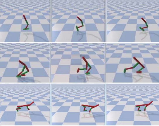
Figure 1. Hopper, Walker2D and HalfCheetah trained agents

4.1. Exploration noise in trials with PyBullet Hopper

The HopperBulletEnv environment is considered solved if the achieved score exceeds $2500$. In TD3 experiments with the HopperBulletEnv environment, I got, among others, the following training curves with $std=0.1$ and $std=0.3$:

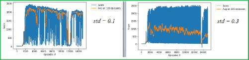
Figure 2. Experiments with Hopper train agent

Here, $std$ is the standard deviation of exploration noise in the TD3. In both trials, the threshold of $2500$ was not reached. However, I noticed the following features:

• In the experiment with $std=0.3$, there are a lot of values near $2500$ (but less than 2500) and at the same time, the average score decreased at all times. This is explained as follows: the number of small score values prevailed over the number of large score values, and the difference between these numbers increased.
  

• In the experiment with $std=0.1$, the average score values reached large values but in general, the average scores decreased. The reason of this, as above, is that the number of small score values prevailed over the number of large score values.
  

• It seems that the prevalence of very small values was due to too high noise standard deviations. Then, the decision was made to reduce $std$ to $0.02$, this was sufficient for solving the environment.

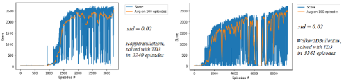
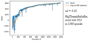
Figure 3. Hopper,Walker2D and HalfCheetah are solved with TD3, see [18]

Appendix A Hill climbing algorithm with adaptive noise

A.1. Forerunner of tensors

We illustrate the properties of the hill climbing algorithm, see [6], applied to the Cartpole environment, [11]. Here, the network model is so simple that it does not use tensors (no PyTorch and no Tensorflow). Only a simple matrix of size [4 x 2] is used here, this is the forerunner of tensors. The hill climbing algorithm seeks to maximize a target function $G_{0}$, which in our particular case is the cumulative discounted reward:

$$G_{0}=R_{1}+\gamma R_{2}+\gamma^{2}R_{3}+\dots=\sum_{k=0}^{\infty}{\gamma}^{k}R_{k+1}$$

where $\gamma$ is the discount factor, $0<\gamma<1$, and $R_{k}$ is the reward obtained at the time step $k$ of the episode. The target function $G_{0}$ appears in Python as follows:

⬇

”’ This is the ’cumulative discounted reward’ or TD-target G_t ”’

Gt = sum([a*b for a,b in zip(discounts, rewards)])

A.2. Two Cartpole environmens

What is $Cartpole$ ? A pole is attached by a joint to a cart, which moves along a track. The system is controlled by applying a force of +1 or -1 to the cart. The pendulum starts upright, and the goal is to prevent it from falling over. A reward of +1 is provided for every timestep that the pole remains upright. The episode ends when the pole $>15$ degrees from a vertical orientation, or the cart moves $>2.4$ units from the center, [12]. The differences between Cartpole-v0 (resp. Cartpole-v1) are in two parameters: the threshold = $195$ (resp. $475$) and the max number of episodes = $200$ (resp $500$). Solving the Cartpole-v0 environment (resp. Cartpole-v1) requires an average total reward that exceeds the threshold for $100$ consecutive episodes.

For GitHub projects that solve both Cartpole-v0 and Cartpole-v1 environments with DQNs and double DQNs, see [16, 17].

A.3. Weight matrix in the hill climbing model

Hill climbing is a simple gradient-free algorithm. We try to climb to the top of a curve by only changing the arguments of the target function $G_{0}$ using a certain adaptive noise. The argument of $G_{0}$ is a weight matrix for determining the neural network that underlies our model.

A.4. Adaptive noise scale

The adaptive noise scale for our model is realized as follows. If the current value of the target function is better than the best value obtained for the target function, we divide the noise scale by $2$, and the corresponding noise is added to the weight matrix. If the current value of the target function is worse than the best obtained value, we multiply the noise scale by $2$, and the corresponding noise is added to the best obtained weight matrix value. In both cases, a noise scale is added with some random factor different for each element of the matrix:

⬇

”’ found better weights ==> decrease the noise: noise = noise/2”’

best_w = policy.w

noise_scale = max(1e-3, noise_scale/2)

policy.w += noise_scale * np.random.rand(*policy.w.shape)

else:

”’ no better weights, increase the noise: noise = noise/2”’

noise_scale = min(2, noise_scale * 2)

policy.w += best_w + noise_scale * np.random.rand(*policy.w.shape)

The Cartpole-v0 environment is solved in $113$ episodes, and Cartpole-v1 is solved in $112$ episodes. For more information on Cartpole-v0/Cartpole-v1 with adaptive noise scaling, see the Jupyter notebooks [16, 17].

A.5. A more generic formula for the noise scale

As seen above, the noise scale adaptively increases or decreases depending on whether the target function is lower or higher than the best obtained value. The noise scale in this algorithm is $2$. In [14], the authors considered more generic formula:

$$\sigma_{k+1}=\left\{\begin{array}[]{ll}&\alpha\sigma_{k}\text{ if }d(\pi,\widetilde{\pi})<\delta,\\ &\\ &\frac{1}{\alpha}\sigma_{k}\text{ otherwise },\end{array}\right.\\$$

where $\alpha$ is a noise scale, $d$ is a certain distance measure between the perturbed and nonperturbed policy, and $\delta$ is a threshold value. In [14, App. C], the authors considered the possible forms of the distance function $d$ for the DQN, DDPG and TPRO algorithms.

References

- []
- [1] S.Thrun and A.Schwartz (1993) Issues in Using Function Approximation for Reinforcement Learning, Carnegie Mellon University, The Robotics Institute
- [2] H.van Hasselt et. al. (2015) Deep Reinforcement Learning with Double Q-learning, arXiv:1509.06461
- [3] T.P.Lillicrap et. al. (2015) Continuous control with deep reinforcement learning, arXiv:1509.02971
- [4] S.Fujimoto et. al. (2018) Addressing Function Approximation Error in Actor-Critic Methods, (2018), arXiv: arXiv:1802.09477v3
- [5] M.Plappert et. al. (2017) Better Exploration with Parameter Noise, OpenAI.com
- [6] B.Mahyavanshi (2019) Introduction to Hill Climbing | Artificial Intelligence, Medium.
- [7] Deep Deterministic Policy Gradient (2018) OpenAI, Spinning Up, Revision 038665d6, https://spinningup.openai.com/en/latest/algorithms/ddpg.html
- [8] Ornstein-Uhlenbeck process, Wikipedia, https://en.wikipedia.org/wiki/Ornstein-Uhlenbeck_process
- [9] Bullet Real-Time Physics Simulation (2020) https://pybullet.org/wordpress/
- [10] Li, M., Huang, T. & Zhu, W. (2022) Adaptive exploration policy for exploration–exploitation tradeoff in continuous action control optimization, Int. J. Mach. Learn. & Cyber. 12, 3491–3501.
- [11] R.Stekolshchik (2020) How does the Bellman equation work in Deep RL?, TowardsDataScience.
- [12] R.Stekolshchik (2020) A pair of interrelated neural networks in Deep Q-Network, TowardsDataScience.
- [13] R.Stekolshchik (2020) Three aspects of Deep RL: noise, overestimation and exploration, TowardsDataScience.
- [14] M.Plappert, et. al. (2017) Parameter Space Noise for Exploration, OpenAI, arXiv:1706.01905v2, ICLR
- [15] Pybullet, Project description (2020), https://pypi.org/project/pybullet/
- [16] R.Stekolshchik (2020) Cartpole with DQN, https://github.com/Rafael1s/Deep-Reinforcement-Learning-Udacity/tree/master/Cartpole-Deep-Q-Learning
-
[17]
R.Stekolshchik (2020) Cartpole with Double Deep Q-Network
https://github.com/Rafael1s/Deep-Reinforcement-Learning-Udacity/tree/master/Cartpole-Double-Deep-Q-Learning -
[18]
R.Stekolshchik (2020) HopperBulletEnv with Twin Delayed DDPG (TD3)
https://github.com/Rafael1s/Deep-Reinforcement-Learning-Udacity/blob/master/HopperBulletEnv_v0-TD3 - []