Scalar scattering amplitude in Gaussian wave-packet formalism

Abstract

We compute an $s$-channel $2\to 2$ scalar scattering $\phi\phi\to\Phi\to\phi\phi$ in the Gaussian wave-packet formalism at the tree-level. We find that wave-packet effects, including shifts of the pole and width of the propagator of $\Phi$, persist even when we do not take into account the time-boundary effect for $2\to 2$, proposed earlier. The result can be interpreted that a heavy scalar $1\to 2$ decay $\Phi\to\phi\phi$, taking into account the production of $\Phi$, does not exhibit the in-state time-boundary effect unless we further take into account in-boundary effects for the $2\to 2$ scattering. We also show various plane-wave limits.

1 Introduction and summary

It is well-known that a plane-wave S-matrix is ill-defined when taken literally because its matrix element is proportional to the energy-momentum delta function, which always gives either zero or infinity when squared to compute a probability. On the other hand, we may define an S-matrix in the Gaussian wave-packet basis without such an infinity [1, 2].

It has been claimed that the Gaussian formalism gives a deviation from the Fermi’s golden rule [3, 4], in which the probability is suppressed only by a power of the deviation from the energy-momentum conservation rather than the conventional exponential suppression; see also Refs. [6, 7, 8].

In Ref. [2], a scalar decay $\Phi\to\phi\phi$ has been computed in the Gaussian formalism, and the previously-claimed power-law deviation from the Fermi’s golden rule has been identified to come from the configuration in which the decay interaction is placed near a time-boundary. As we will see, this configuration is realized, even if the in/out states are at a distance. To examine the in-boundary effect for $1\to 2$ more in detail, it is desirable to take into account the production process of the decaying $\Phi$.

In this paper, we compute a tree-level $s$-channel scalar scattering $\phi\phi\to\Phi\to\phi\phi$ in the Gaussian formalism. We find that wave-packet effects, including shifts of the pole and width of the propagator of $\Phi$, persists even when we do not take into account the time-boundary effect, proposed earlier. The result can be interpreted that a heavy scalar decay $\Phi\to\phi\phi$, taking into account the production of $\Phi$, does not exhibit the in-state $1\to 2$ time-boundary effect unless we take into account the in-state $2\to 2$ time boundary.

This paper is organized as follows: In Sec. 2, we present basic setup of the Gaussian formalism, and compute the Gaussian S-matrix for the $s$-channel $2\to 2$ scattering: $\phi\phi\to\Phi\to\phi\phi$. In Sec. 3, we discuss the possible time-boundary effects. In Sec. 4, we focus on the bulk contribution and show that wave effects exist even when we neglect the boundary contributions. In Sec. 5, we present several plane-wave limits of the obtained result. In Sec. 6, we present summary and discussion. In Appendix A, we compare with the $\phi\phi\to\phi\phi$ scattering in the $\phi^{4}$ theory.

2 Gaussian S-matrix

Here we first review the Gaussian formalism, and obtain the S-matrix for the $s$-channel $2\to 2$ scalar scattering: $\phi\phi\to\Phi\to\phi\phi$.

2.1 Gaussian basis

We review the Gaussian formalism, following Ref. [2], to clarify the notation in this paper. A free scalar field operator $\hat{\varphi}$ at $x=\left(x^{0},\boldsymbol{x}\right)$ (in the interaction picture) can be expanded by the plane basis:

$$\hat{\varphi}\!\left(x\right) =\left.\int{\text{d}^{3}\boldsymbol{p}\over\sqrt{2p^{0}}\left(2\pi\right)^{3/2}}\left[e^{ip\cdot x}\hat{a}_{\varphi}\!\left(\boldsymbol{p}\right)+\text{h.c.}\right]\right|_{p^{0}=E_{\varphi}\!\left(\boldsymbol{p}\right)}$$

$$=\left.\int{\text{d}^{3}\boldsymbol{p}\over\sqrt{2p^{0}}}\left[\Braket{\varphi;x}{\varphi;\boldsymbol{p}}\hat{a}_{\varphi}\!\left(\boldsymbol{p}\right)+\text{h.c.}\right]\right|_{p^{0}=E_{\varphi}\!\left(\boldsymbol{p}\right)},$$ (1)

where $\varphi=\phi,\Phi$ labels the particle species; $\hat{a}_{\varphi}\!\left(\boldsymbol{p}\right)$ and $\hat{a}_{\varphi}^{\dagger}\!\left(\boldsymbol{p}\right)$ are the annihilation and creation operators, respectively, with

$$\left[\hat{a}_{\varphi}\!\left(\boldsymbol{p}\right),\hat{a}_{\varphi^{\prime}}^{\dagger}\!\left(\boldsymbol{p}^{\prime}\right)\right] =\delta_{\varphi\varphi^{\prime}}\delta^{3}\!\left(\boldsymbol{p}-\boldsymbol{p}^{\prime}\right), =0;$$ others (2)

and

$$E_{\varphi}\!\left(\boldsymbol{p}\right) :=\sqrt{m_{\varphi}^{2}+\boldsymbol{p}^{2}},$$ (3)

$$\Ket{\varphi;\boldsymbol{p}} :=\hat{a}^{\dagger}_{\varphi}\!\left(\boldsymbol{p}\right)\Ket{0},$$ (4)

$$\Braket{\varphi;\boldsymbol{x}}{\varphi^{\prime};\boldsymbol{p}} :=\delta_{\varphi\varphi^{\prime}}{e^{i\boldsymbol{p}\cdot\boldsymbol{x}}\over\left(2\pi\right)^{3/2}},$$ (5)

$$\Ket{\varphi;x} :=e^{+i\hat{H}_{\text{free}}t}\Ket{\varphi;\boldsymbol{x}},$$ (6)

with $\hat{H}_{\text{free}}$ being the free Hamiltonian:

$$\hat{H}_{\text{free}}\Ket{\varphi;\boldsymbol{p}} =E_{\varphi}\!\left(\boldsymbol{p}\right)\Ket{\varphi;\boldsymbol{p}}.$$ (7)

Here and hereafter, we use $t,T$ and $x^{0},X^{0}$ interchangeably: $t=x^{0}$ and $T=X^{0}$. Note that $\Ket{\varphi;\boldsymbol{x}}$ and $\Ket{\varphi;\boldsymbol{p}}$ are independent of time and hence can be regarded as either a Heisenberg-picture state or a Schrödinger-picture eigenbasis (of total Hamiltonian), while $\Ket{\varphi;x}$ is an interaction-picture basis at time $x^{0}$ as seen from its time evolution by the free Hamiltonian.

We define a Gaussian wave-packet state $\Ket{\varphi,\sigma;\boldsymbol{\Pi}}$ by

$$\Braket{\varphi^{\prime},\boldsymbol{x}}{\varphi,\sigma;\boldsymbol{\Pi}} :={1\over\left(\pi\sigma\right)^{3/4}}e^{i\boldsymbol{P}\cdot\left(\boldsymbol{x}-\boldsymbol{X}\right)}e^{-{1\over 2\sigma}\left(\boldsymbol{x}-\boldsymbol{X}\right)^{2}}\delta_{\varphi\varphi^{\prime}},$$ (8)

where $\boldsymbol{\Pi}:=\left(\boldsymbol{X},\boldsymbol{P}\right)$ gives the center of wave packet in the phase space. Note that

$$\Braket{\varphi^{\prime},\boldsymbol{p}}{\varphi,\sigma;\boldsymbol{\Pi}} =\delta_{\varphi\varphi^{\prime}}\left(\sigma\over\pi\right)^{3/4}e^{-i\boldsymbol{p}\cdot\boldsymbol{X}}e^{-{\sigma\over 2}\left(\boldsymbol{p}-\boldsymbol{P}\right)^{2}},$$ (9)

$$\Braket{\varphi,\sigma;\boldsymbol{\Pi}}{\varphi^{\prime},\sigma^{\prime};\boldsymbol{\Pi}^{\prime}} =\left(\sigma_{\text{I}}\over\sigma_{\text{A}}\right)^{3/4}e^{-{1\over 4\sigma_{\text{A}}}\left(\boldsymbol{X}-\boldsymbol{X}^{\prime}\right)^{2}}e^{-{\sigma_{\text{I}}\over 4}\left(\boldsymbol{P}-\boldsymbol{P}^{\prime}\right)^{2}}e^{{i\over 2\sigma_{\text{I}}}\left(\sigma\boldsymbol{P}+\sigma^{\prime}\boldsymbol{P}^{\prime}\right)\cdot\left(\boldsymbol{X}-\boldsymbol{X}^{\prime}\right)}\delta_{\varphi\varphi^{\prime}},$$ (10)

where

$$\sigma_{\text{A}} :={\sigma+\sigma^{\prime}\over 2}, \sigma_{\text{I}} :=\left(\sigma^{-1}+\sigma^{\prime-1}\over 2\right)^{-1}={2\sigma\sigma^{\prime}\over\sigma+\sigma^{\prime}},$$ (11)

are the average and the inverse of average of inverse, respectively. Especially,

$$\Braket{\varphi,\sigma;\boldsymbol{\Pi}}{\varphi,\sigma;\boldsymbol{\Pi}^{\prime}} =e^{-{1\over 4\sigma}\left(\boldsymbol{X}-\boldsymbol{X}^{\prime}\right)^{2}}e^{-{\sigma\over 4}\left(\boldsymbol{P}-\boldsymbol{P}^{\prime}\right)^{2}}e^{{i\over 2}\left(\boldsymbol{P}+\boldsymbol{P}^{\prime}\right)\cdot\left(\boldsymbol{X}-\boldsymbol{X}^{\prime}\right)}.$$ (12)

The state $\Ket{\varphi,\sigma;\boldsymbol{\Pi}}$ is time independent and hence can be regarded as either a Heisenberg state or a Schrödinger basis. We also define the interaction basis at time $X^{0}$:

$$\Ket{\varphi,\sigma;\Pi} :=e^{i\hat{H}_{\text{free}}X^{0}}\Ket{\varphi,\sigma;\boldsymbol{\Pi}},$$ (13)

where $\Pi:=\left(X,\boldsymbol{P}\right)=\left(X^{0},\boldsymbol{X},\boldsymbol{P}\right)=\left(X^{0},\boldsymbol{\Pi}\right)$. As we will see later, we will treat $\Ket{\varphi,\sigma;\Pi}$ as a time-independent Heisenberg state (or equivalently a time-independent Schrödinger basis).

We define a creation operator of the Gaussian basis by

$$\hat{A}_{\varphi,\sigma}^{\dagger}\!\left(\Pi\right)\Ket{0} :=\Ket{\varphi,\sigma;\Pi},$$ (14)

which results in $\hat{A}_{\varphi,\sigma}\!\left(\Pi\right)\Ket{0}=0$ and

$$\left[\hat{A}_{\varphi,\sigma}\!\left(\Pi\right),\hat{A}^{\dagger}_{\varphi^{\prime},\sigma^{\prime}}\!\left(\Pi^{\prime}\right)\right] =\Braket{\varphi,\sigma,\Pi}{\varphi^{\prime},\sigma^{\prime};\Pi^{\prime}}, =0.$$ others (15)

We may also expand $\hat{\varphi}$ by the creation and annihilation operators of the free Gaussian wave packets:

$$\hat{\varphi}\!\left(x\right) =\int{\text{d}^{3}\boldsymbol{X}\,\text{d}^{3}\boldsymbol{P}\over\left(2\pi\right)^{3}}\left[f_{\varphi,\sigma;X,\boldsymbol{P}}\!\left(x\right)\hat{A}_{\varphi,\sigma}\!\left(X,\boldsymbol{P}\right)+\text{h.c.}\right],$$ (16)

where $X=\left(X^{0},\boldsymbol{X}\right)$ is the center of the wave packet; $\boldsymbol{P}$ is the central momentum of the wave packet; $\sigma$ and $X^{0}$ are fixed (and can differ) for each field participating in the scattering; and the coefficient function becomes

$$f_{\varphi,\sigma;X,\boldsymbol{P}}\!\left(x\right) :=\int{\text{d}^{3}\boldsymbol{p}\over\sqrt{2E_{\varphi}\!\left(\boldsymbol{p}\right)}}\Braket{\varphi;x}{\varphi;\boldsymbol{p}}\Braket{\varphi;\boldsymbol{p}}{\varphi,\sigma;\Pi}$$

$$=\left.\left(\sigma\over\pi\right)^{3/4}\int{\text{d}^{3}\boldsymbol{p}\over\sqrt{2p^{0}}\left(2\pi\right)^{3/2}}e^{ip\cdot\left(x-X\right)-{\sigma\over 2}\left(\boldsymbol{p}-\boldsymbol{P}\right)^{2}}\right|_{p^{0}=E_{\varphi}\!\left(\boldsymbol{p}\right)}.$$ (17)

We also write

$$\text{d}^{6}\boldsymbol{\Pi} :={\text{d}^{3}\boldsymbol{X}\,\text{d}^{3}\boldsymbol{P}\over\left(2\pi\right)^{3}}$$ (18)

so that

$$\hat{\varphi}\!\left(x\right) =\int\text{d}^{6}\boldsymbol{\Pi}\left[f_{\varphi,\sigma;\Pi}\!\left(x\right)\hat{A}_{\varphi,\sigma}\!\left(\Pi\right)+\text{h.c.}\right].$$ (19)

By e.g. sandwiching between $\Bra{\boldsymbol{p}}$ and $\Ket{\boldsymbol{p}^{\prime}}$, we can show the completeness of the Gaussian basis in the one-particle subspace:

$$\int\text{d}^{6}\boldsymbol{\Pi}\Ket{\varphi,\sigma;\Pi}\Bra{\varphi,\sigma;\Pi} =\hat{1}.$$ (20)

Namely, the Gaussian basis can expand any one-particle wave function $\psi\!\left(\boldsymbol{x}\right)=\Braket{\boldsymbol{x}}{\psi}$ as

$$\Braket{\boldsymbol{x}}{\psi} =\int\text{d}^{6}\boldsymbol{\Pi}\Braket{\boldsymbol{x}}{\boldsymbol{\Pi}}\Braket{\boldsymbol{\Pi}}{\psi},$$ (21)

where we used the short-hand notation $\Ket{\boldsymbol{\Pi}}=\Ket{\varphi,\sigma;\boldsymbol{\Pi}}$ etc. and $\Braket{\boldsymbol{x}}{\boldsymbol{\Pi}}$ is given in Eq. (8). We have also used $\Ket{\Pi}\Bra{\Pi}=\Ket{\boldsymbol{\Pi}}\Bra{\boldsymbol{\Pi}}$ from Eq. (13). Note the following relation:

$$\Bra{0}\hat{A}_{\varphi,\sigma}\!\left(\Pi\right)\hat{A}_{\varphi^{\prime},\sigma^{\prime}}^{\dagger}\!\left(\Pi^{\prime}\right)\Ket{0} =\Braket{\varphi,\sigma;\Pi}{\varphi,\sigma^{\prime};\Pi^{\prime}}\delta_{\varphi\varphi^{\prime}},$$ (22)

$$\left.\Braket{\varphi,\sigma;\Pi}{\varphi,\sigma;\Pi^{\prime}}\right|_{X^{0}=X^{\prime 0}} =e^{-{1\over 4\sigma}\left(\boldsymbol{X}-\boldsymbol{X}^{\prime}\right)^{2}}e^{-{\sigma\over 4}\left(\boldsymbol{P}-\boldsymbol{P}^{\prime}\right)^{2}}e^{{i\over 2}\left(\boldsymbol{P}+\boldsymbol{P}^{\prime}\right)\cdot\left(\boldsymbol{X}-\boldsymbol{X}^{\prime}\right)}.$$ (23)

In the large-$\sigma$ expansion, we get

$$f_{\varphi,\sigma;X,\boldsymbol{P}}\!\left(x\right) \to\left.\left(\sigma\over\pi\right)^{3/4}\left(2\pi\over\sigma\right)^{3/2}{1\over\sqrt{2P^{0}}\left(2\pi\right)^{3/2}}e^{iP\cdot\left(x-X\right)-{\left(\boldsymbol{x}-\boldsymbol{\Xi}_{\varphi}^{\Pi}\!\left(x^{0}\right)\right)^{2}\over 2\sigma}}\right|_{P^{0}=E_{\varphi}\!\left(\boldsymbol{P}\right)},$$ (24)

where

$$\boldsymbol{\Xi}^{\Pi}_{\varphi}\!\left(x^{0}\right) :=\boldsymbol{\mathfrak{X}}_{\varphi}^{\Pi}+\boldsymbol{V}_{\varphi}\!\left(\boldsymbol{P}\right)x^{0}$$

$$=\boldsymbol{X}+\boldsymbol{V}_{\varphi}\!\left(\boldsymbol{P}\right)\left(x^{0}-X^{0}\right),$$ (25)

in which

$$\boldsymbol{\mathfrak{X}}_{\varphi}^{\Pi} :=\boldsymbol{X}-\boldsymbol{V}_{\varphi}\!\left(\boldsymbol{P}\right)X^{0}, \boldsymbol{V}_{\varphi}\!\left(\boldsymbol{P}\right) :={\boldsymbol{P}\over E_{\varphi}\!\left(\boldsymbol{P}\right)}.$$ (26)

2.2 In and out states

We consider the $s$-channel scalar scattering $\phi\phi\to\Phi\to\phi\phi$. Since both the in and out states are of $\phi$, we omit the label $\phi$ hereafter.

Generically, one particle in the in- and out-states can be asymptotic to an arbitrary free wave function $\Psi\!\left(x\right)=\Braket{x}{\Psi}$, which can be expanded by the Gaussian basis as

$$\Ket{\Psi} =\int\text{d}^{6}\boldsymbol{\Pi}\,\Ket{\boldsymbol{\Pi}}\Braket{\boldsymbol{\Pi}}{\Psi}.$$ (27)

Therefore without loss of generality, we may assume that the asymptotic free states are Gaussian, and we will do so hereafter.

We prepare the in and out Heisenberg states $\Ket{\text{in};\sigma_{1},\Pi_{1};\sigma_{2},\Pi_{2}}$ and $\Ket{\text{out};\sigma_{3},\Pi_{3};\sigma_{4},\Pi_{4}}$, respectively, by

$$e^{-i\hat{H}t}\Ket{\text{in};\sigma_{1},\Pi_{1};\sigma_{2},\Pi_{2}} \to e^{-i\hat{H}_{\text{free}}t}\Ket{\sigma_{1},\Pi_{1};\sigma_{2},\Pi_{2}} (t \to T_{\text{in}}),$$

$$e^{-i\hat{H}t}\Ket{\text{out};\sigma_{3},\Pi_{3};\sigma_{4},\Pi_{4}} \to e^{-i\hat{H}_{\text{free}}t}\Ket{\sigma_{3},\Pi_{3};\sigma_{4},\Pi_{4}} (t \to T_{\text{out}}),$$ (28)

where we have defined the free states

$$\Ket{\sigma_{1},\Pi_{1};\sigma_{2},\Pi_{2}} :=\hat{A}^{\dagger}_{\sigma_{1}}\!\left(\Pi_{1}\right)\hat{A}^{\dagger}_{\sigma_{2}}\!\left(\Pi_{2}\right)\Ket{0},$$ (29)

etc., and take

$$T_{\text{in}} \lesssim\max\!\left(X_{1}^{0},X_{2}^{0}\right), T_{\text{out}} \gtrsim\min\!\left(X_{3}^{0},X_{4}^{0}\right).$$ (30)

See Sec. 3 for further discussion.

2.3 Gaussian two-point function

In this subsection, we omit the labels $\varphi$ and $\sigma$ as they are all equal, except for the mass $m_{\varphi}$. In the later application, $\varphi$ will be the intermediate heavy scalar $\Phi$.

We want to put the expansion (19), into the time-ordered two-point function:

$$\Bra{0}\operatorname{T}\hat{\varphi}\!\left(x\right)\hat{\varphi}\!\left(x^{\prime}\right)\Ket{0} =\theta\!\left(x^{0}-x^{\prime 0}\right)\Bra{0}\hat{\varphi}\!\left(x\right)\hat{\varphi}\!\left(x^{\prime}\right)\Ket{0}+\theta\!\left(x^{\prime 0}-x^{0}\right)\Bra{0}\hat{\varphi}\!\left(x^{\prime}\right)\hat{\varphi}\!\left(x\right)\Ket{0}.$$ (31)

Now we can check that

$$\Bra{0}\hat{\varphi}\!\left(x\right)\hat{\varphi}\!\left(x^{\prime}\right)\Ket{0} =\hbox to0.0pt{$\displaystyle\int\text{d}^{6}\boldsymbol{\Pi}\,\int\text{d}^{6}\boldsymbol{\Pi}^{\prime}\,f_{\Pi}\!\left(x\right)f^{*}_{\Pi^{\prime}}\!\left(x^{\prime}\right)\Bra{0}\hat{A}\!\left(\Pi\right)\hat{A}^{\dagger}\!\left(\Pi^{\prime}\right)\Ket{0}$\hss}$$

$$=\int{\text{d}^{3}\boldsymbol{p}\over\sqrt{2E\!\left(\boldsymbol{p}\right)}}\int{\text{d}^{3}\boldsymbol{p}^{\prime}\over\sqrt{2E\!\left(\boldsymbol{p}^{\prime}\right)}}\int\text{d}^{6}\boldsymbol{\Pi}\,\int\text{d}^{6}\boldsymbol{\Pi}^{\prime}$$

$$\quad\times\Braket{x}{\boldsymbol{p}}\Braket{\boldsymbol{p}}{\Pi}\Braket{\Pi}{\Pi^{\prime}}\Braket{\Pi^{\prime}}{\boldsymbol{p}^{\prime}}\Braket{\boldsymbol{p}^{\prime}}{x^{\prime}}$$

$$=\int{\text{d}^{3}\boldsymbol{p}\over 2E\!\left(\boldsymbol{p}\right)}\Braket{x}{\boldsymbol{p}}\Braket{\boldsymbol{p}}{x^{\prime}}=\left.\int{\text{d}^{3}\boldsymbol{p}\over 2E\!\left(\boldsymbol{p}\right)\left(2\pi\right)^{3}}e^{ip\cdot\left(x-x^{\prime}\right)}\right|_{p^{0}=E\!\left(\boldsymbol{p}\right)}.$$ (32)

Putting this into the two-point function (31),

$$\Bra{0}\operatorname{T}\hat{\varphi}\!\left(x\right)\hat{\varphi}\!\left(x^{\prime}\right)\Ket{0} =\left.\int{\text{d}^{3}\boldsymbol{p}\over 2E\!\left(\boldsymbol{p}\right)\left(2\pi\right)^{3}}\left(\theta\!\left(x^{0}-x^{\prime 0}\right)e^{ip\cdot\left(x-x^{\prime}\right)}+\theta\!\left(x^{\prime 0}-x^{0}\right)e^{ip\cdot\left(x^{\prime}-x\right)}\right)\right|_{p^{0}=E\!\left(\boldsymbol{p}\right)}.$$ (33)

We have recovered the ordinary plane-wave propagator as we should, since we integrate over the complete set. As usual, using

$$\theta\!\left(x^{0}\right) =-{1\over 2\pi i}\int_{-\infty}^{\infty}\text{d}\omega{e^{-i\omega x^{0}}\over\omega+i\epsilon},$$ (34)

with $\epsilon$ being an arbitrary positive infinitesimal, we may rewrite it into more familiar form:

$$\Bra{0}\operatorname{T}\hat{\varphi}\!\left(x\right)\hat{\varphi}\!\left(x^{\prime}\right)\Ket{0} =\int{\text{d}^{3}\boldsymbol{p}\,e^{i\boldsymbol{p}\cdot\left(\boldsymbol{x}-\boldsymbol{x}^{\prime}\right)}\over 2E\!\left(\boldsymbol{p}\right)\left(2\pi\right)^{3}}$$

$$\quad\times\left(-\int_{-\infty}^{\infty}{\text{d}\omega\over 2\pi i}{e^{-i\left(\omega+E\!\left(\boldsymbol{p}\right)\right)\left(x^{0}-x^{\prime 0}\right)}\over\omega+i\epsilon}-\int_{-\infty}^{\infty}{\text{d}\omega\over 2\pi i}{e^{-i\left(\omega-E\!\left(\boldsymbol{p}\right)\right)\left(x^{0}-x^{\prime 0}\right)}\over-\omega+i\epsilon}\right)$$

$$={i\over\left(2\pi\right)^{4}}\int{\text{d}^{3}\boldsymbol{p}\over 2E\!\left(\boldsymbol{p}\right)}\int_{-\infty}^{\infty}\text{d}p^{0}\,e^{ip\cdot\left(x-x^{\prime}\right)}$$

$$\quad\times\left({1\over p^{0}-E\!\left(\boldsymbol{p}\right)+i\epsilon}+{1\over-p^{0}-E\!\left(\boldsymbol{p}\right)+i\epsilon}\right)$$

$$={i\over\left(2\pi\right)^{4}}\int\text{d}^{3}\boldsymbol{p}\int_{-\infty}^{\infty}\text{d}p^{0}\,e^{ip\cdot\left(x-x^{\prime}\right)}{-1\over\left(\boldsymbol{p}^{2}+m_{\varphi}^{2}-i\epsilon\right)-\left(p^{0}\right)^{2}}$$

$$=-i\int{\text{d}^{4}p\over\left(2\pi\right)^{4}}{e^{ip\cdot\left(x-x^{\prime}\right)}\over p^{2}+m_{\varphi}^{2}-i\epsilon}=-i\Delta_{\text{F}}\!\left(x-x^{\prime}\right).$$ (35)

2.4 Gaussian S-matrix

Now we compute the probability amplitude under the assumption (28):

$$\mathcal{S} =\Braket{\text{out};\sigma_{3},\Pi_{3};\sigma_{4};\Pi_{4}}{\text{in};\sigma_{1},\Pi_{1};\sigma_{2},\Pi_{2}}$$

$$=\Bra{\sigma_{3},\Pi_{3};\sigma_{4},\Pi_{4}}e^{i\hat{H}_{\text{free}}T_{\text{out}}}e^{-i\hat{H}T_{\text{out}}}e^{i\hat{H}T_{\text{in}}}e^{-i\hat{H}_{\text{free}}T_{\text{in}}}\Ket{\sigma_{1},\Pi_{1};\sigma_{2},\Pi_{2}}$$

$$=\Bra{\sigma_{3},\Pi_{3};\sigma_{4},\Pi_{4}}\operatorname{T}\exp\!\left(-i\int_{T_{\text{in}}}^{T_{\text{out}}}\text{d}t\,\hat{H}^{\text{I}}_{\text{int}}\!\left(t\right)\right)\Ket{\sigma_{1},\Pi_{1};\sigma_{2},\Pi_{2}}$$

$$=:\Bra{\sigma_{3},\Pi_{3};\sigma_{4},\Pi_{4}}\hat{S}\Ket{\sigma_{1},\Pi_{1};\sigma_{2},\Pi_{2}},$$ (36)

where $\hat{H}^{\text{I}}_{\text{int}}\!\left(t\right)=e^{i\hat{H}_{\text{free}}t}\left(\hat{H}-\hat{H}_{\text{free}}\right)e^{-i\hat{H}_{\text{free}}t}$ is the interaction Hamiltonian in the interaction picture. In the plane-wave S-matrix, one subtracts the first term in the Dyson series (36), write $\hat{S}=\hat{1}+i\hat{T}$, and concentrate on the transition amplitude from $\hat{T}$. In the Gaussian formalism, we do not need such regularization of dropping the first term $\hat{1}$ because the inner product of the free states would remain finite even for identical momenta. When we integrate over the final state momenta $\boldsymbol{P}_{3}$ and $\boldsymbol{P}_{4}$, the contribution from $\hat{1}$ would automatically drop out even if we take the plane-wave limit after all the computations. Hereafter, we omit the trivial term $\Braket{\sigma_{3},\Pi_{3};\sigma_{4},\Pi_{4}}{\sigma_{1},\Pi_{1};\sigma_{2},\Pi_{2}}$ from $\mathcal{S}$ when we call it “transition amplitude”.

In this paper, we consider the following simplest interaction Hamiltonian:

$$\hat{H}_{\text{int}}^{\text{I}}\!\left(t\right) ={\kappa\over 2}\int\text{d}^{3}\boldsymbol{x}\,\hat{\phi}^{2}\!\left(x\right)\hat{\Phi}\!\left(x\right),$$ (37)

where $\hat{\phi}$ and $\hat{\Phi}$ are given in Eq. (1). The tree-level transition amplitude is given by

$$\mathcal{S} ={\left(-i\kappa\right)^{2}\over 8}\int_{T_{\text{in}}}^{T_{\text{out}}}\text{d}t\int\text{d}^{3}\boldsymbol{x}\int_{T_{\text{in}}}^{T_{\text{out}}}\text{d}t^{\prime}\int\text{d}^{3}\boldsymbol{x}^{\prime}$$

$$\quad\times\Bra{0}\operatorname{T}_{x,x^{\prime}}\hat{A}_{\sigma_{3}}\!\left(\Pi_{3}\right)\hat{A}_{\sigma_{4}}\!\left(\Pi_{4}\right)\hat{\phi}\!\left(x\right)\hat{\phi}\!\left(x\right)\hat{\Phi}\!\left(x\right)\hat{\phi}\!\left(x^{\prime}\right)\hat{\phi}\!\left(x^{\prime}\right)\hat{\Phi}\!\left(x^{\prime}\right)\hat{A}^{\dagger}_{\sigma_{1}}\!\left(\Pi_{1}\right)\hat{A}^{\dagger}_{\sigma_{2}}\!\left(\Pi_{2}\right)\Ket{0},$$ (38)

where $\operatorname{T}_{x,x^{\prime}}$ is the time ordering with respect to $x$ and $x^{\prime}$ only. Hereafter, we concentrate on the $s$-channel process because it is dominant in the near on-shell process of our interest.

For example, a part of the $s$-channel process is

$$\mathcal{S} \supset{\left(-i\kappa\right)^{2}\over 8}\int_{T_{\text{in}}}^{T_{\text{out}}}\text{d}t\int\text{d}^{3}\boldsymbol{x}\int_{T_{\text{in}}}^{T_{\text{out}}}\text{d}t^{\prime}\int\text{d}^{3}\boldsymbol{x}^{\prime}$$

The Wick contraction with the external line gives, for example,

$$\contraction{}{\hat{A}}{{}_{\sigma_{3}}\!\left(\Pi_{3}\right)}{\hat{\phi}}\hat{A}_{\sigma_{3}}\!\left(\Pi_{3}\right)\hat{\phi}\!\left(x\right) =\int\text{d}^{6}\boldsymbol{\Pi}f^{*}_{\sigma;\Pi}\!\left(x\right)\left[\hat{A}_{\sigma_{3}}\!\left(\Pi_{3}\right),\hat{A}^{\dagger}_{\sigma}\!\left(\Pi\right)\right]$$

$$=\int\text{d}^{6}\boldsymbol{\Pi}\int{\text{d}^{3}\boldsymbol{p}\over\sqrt{2E_{\phi}\!\left(\boldsymbol{p}\right)}}\Braket{\sigma;\Pi}{\phi,\boldsymbol{p}}\Braket{\phi,\boldsymbol{p}}{\phi,x}\Braket{\sigma_{3};\Pi_{3}}{\phi,\sigma;\Pi}$$

$$=\int{\text{d}^{3}\boldsymbol{p}\over\sqrt{2E_{\phi}\!\left(\boldsymbol{p}\right)}}\Braket{\sigma_{3};\Pi_{3}}{\phi,\boldsymbol{p}}\Braket{\phi,\boldsymbol{p}}{\phi,x}$$

$$=f^{*}_{\sigma_{3};\Pi_{3}}\!\left(x\right),$$ (39)

where the propagator of $\Phi$ becomes the same as the plane-wave one, as we have seen in the previous sub-section. Then the contribution (LABEL:a_contribution) becomes

$$\mathcal{S} \supset{\left(-i\kappa\right)^{2}\over 8}\int_{T_{\text{in}}}^{T_{\text{out}}}\text{d}t\int\text{d}^{3}\boldsymbol{x}\int_{T_{\text{in}}}^{T_{\text{out}}}\text{d}t^{\prime}\int\text{d}^{3}\boldsymbol{x}^{\prime}$$

$$\quad\times f_{\sigma_{1};\Pi_{1}}\!\left(x^{\prime}\right)f_{\sigma_{2};\Pi_{2}}\!\left(x^{\prime}\right)f^{*}_{\sigma_{3};\Pi_{3}}\!\left(x\right)f^{*}_{\sigma_{4};\Pi_{4}}\!\left(x\right)\Bra{0}\operatorname{T}\bcontraction{}{\hat{\Phi}}{\!\left(x\right)}{\hat{\Phi}}\hat{\Phi}\!\left(x\right)\hat{\Phi}\!\left(x^{\prime}\right)\Ket{0}.$$ (40)

In total there will be factor 8 from the other Wick contractions. To summarize,

$$\mathcal{S} =\left(-i\kappa\right)^{2}\left(-i\right)\int{\text{d}^{4}p\over\left(2\pi\right)^{4}}{1\over p^{2}+M^{2}-i\epsilon}$$

$$\quad\times\int_{T_{\text{in}}}^{T_{\text{out}}}\text{d}t\int\text{d}^{3}\boldsymbol{x}\,f^{*}_{\sigma_{3};\Pi_{3}}\!\left(x\right)f^{*}_{\sigma_{4};\Pi_{4}}\!\left(x\right)e^{ip\cdot x}$$

$$\quad\times\int_{T_{\text{in}}}^{T_{\text{out}}}\text{d}t^{\prime}\int\text{d}^{3}\boldsymbol{x}^{\prime}\,f_{\sigma_{1};\Pi_{1}}\!\left(x^{\prime}\right)f_{\sigma_{2};\Pi_{2}}\!\left(x^{\prime}\right)e^{-ip\cdot x^{\prime}},$$ (41)

where $t:=x^{0}$ and $t^{\prime}:=x^{\prime 0}$ are the production and decay times of $\Phi$, and $M:=m_{\Phi}$ is the heavy scalar mass. This is the starting equation for our computation.

Hereafter, we consider the leading approximation in the plane-wave limit (24):

$$f_{\phi,\sigma_{1};\Pi_{1}}\!\left(x\right)f_{\phi,\sigma_{2};\Pi_{2}}\!\left(x\right) \to\left(1\over\pi\sigma_{1}\right)^{3/4}\left(1\over\pi\sigma_{2}\right)^{3/4}{1\over\sqrt{2E_{1}}\sqrt{2E_{2}}}$$

$$\quad\times e^{iP_{1}\cdot\left(x-X_{1}\right)-{\left(\boldsymbol{x}-\boldsymbol{\Xi}_{1}\!\left(t\right)\right)^{2}\over 2\sigma_{1}}}e^{iP_{2}\cdot\left(x-X_{2}\right)-{\left(\boldsymbol{x}-\boldsymbol{\Xi}_{2}\!\left(t\right)\right)^{2}\over 2\sigma_{2}}},$$

$$f^{*}_{\phi,\sigma_{3};\Pi_{3}}\!\left(x\right)f^{*}_{\phi,\sigma_{4};\Pi_{4}}\!\left(x\right) \to\left(1\over\pi\sigma_{3}\right)^{3/4}\left(1\over\pi\sigma_{4}\right)^{3/4}{1\over\sqrt{2E_{3}}\sqrt{2E_{4}}}$$

$$\quad\times e^{-iP_{3}\cdot\left(x-X_{3}\right)-{\left(\boldsymbol{x}-\boldsymbol{\Xi}_{3}\!\left(t\right)\right)^{2}\over 2\sigma_{3}}}e^{-iP_{4}\cdot\left(x-X_{4}\right)-{\left(\boldsymbol{x}-\boldsymbol{\Xi}_{4}\!\left(t\right)\right)^{2}\over 2\sigma_{4}}},$$ (42)

where for $a=1,\dots,4$,

$$\boldsymbol{\Xi}_{a}\!\left(t\right) :=\boldsymbol{\mathfrak{X}}_{a}+\boldsymbol{V}_{a}t,$$ (43)

in which $\boldsymbol{\mathfrak{X}}_{a}$ is the center of wave packet at a reference time $t=0$ and $\boldsymbol{V}_{a}$ is its central velocity:

$$\boldsymbol{\mathfrak{X}}_{a} :=\boldsymbol{X}_{a}-\boldsymbol{V}_{a}T_{a},$$ (44)

$$\boldsymbol{V}_{a} :={\boldsymbol{P}_{a}\over E_{a}}={\boldsymbol{P}_{a}\over\sqrt{m^{2}+\boldsymbol{P}_{a}^{2}}},$$ (45)

with $m:=m_{\phi}$.

We perform the Gaussian integral over the positions of interaction to get

$$\mathcal{S} =i\kappa^{2}\left(\prod_{A=1}^{4}{1\over\sqrt{2E_{A}}}\left(1\over\pi\sigma_{A}\right)^{3/4}\right)\left(2\pi\sigma_{\text{in}}\right)^{3/2}\left(2\pi\sigma_{\text{out}}\right)^{3/2}\int{\text{d}^{4}p\over\left(2\pi\right)^{4}}{1\over p^{2}+M^{2}-i\epsilon}$$

$$\quad\times\int_{T_{\text{in}}}^{T_{\text{out}}}\text{d}t\,e^{-{\sigma_{\text{out}}\over 2}\left(\boldsymbol{p}-\boldsymbol{P}_{\text{out}}\right)^{2}-{1\over 2\varsigma_{\text{out}}}\left(t-\mathfrak{T}_{\text{out}}\right)^{2}-{\mathcal{R}_{\text{out}}\over 2}-it\left(p^{0}-E_{\text{out}}\right)+i\overline{\boldsymbol{V}}_{\text{out}}\cdot\left(\boldsymbol{p}-\boldsymbol{P}_{\text{out}}\right)t+i\overline{\boldsymbol{\mathfrak{X}}}_{\text{out}}\cdot\left(\boldsymbol{p}-\boldsymbol{P}_{\text{out}}\right)}$$

$$\quad\times\int_{T_{\text{in}}}^{T_{\text{out}}}\text{d}t^{\prime}\,e^{-{\sigma_{\text{in}}\over 2}\left(\boldsymbol{p}-\boldsymbol{P}_{\text{in}}\right)^{2}-{1\over 2\varsigma_{\text{in}}}\left(t^{\prime}-\mathfrak{T}_{\text{in}}\right)^{2}-{\mathcal{R}_{\text{in}}\over 2}+it^{\prime}\left(p^{0}-E_{\text{in}}\right)-i\overline{\boldsymbol{V}}_{\text{in}}\cdot\left(\boldsymbol{p}-\boldsymbol{P}_{\text{in}}\right)t^{\prime}-i\overline{\boldsymbol{\mathfrak{X}}}_{\text{in}}\cdot\left(\boldsymbol{p}-\boldsymbol{P}_{\text{in}}\right)},$$ (46)

where we have dropped a phase factor that cancels out in the square $\left|S\right|^{2}$ and have defined the following:

• Energies and momanta for in and out states:

  $$E_{\text{in}} :=E_{1}+E_{2}, \boldsymbol{P}_{\text{in}} :=\boldsymbol{P}_{1}+\boldsymbol{P}_{2},$$ (47)

  $$E_{\text{out}} :=E_{3}+E_{4}, \boldsymbol{P}_{\text{out}} :=\boldsymbol{P}_{3}+\boldsymbol{P}_{4}.$$ (48)

• The averaged space-like width-squared of the in- and out-states, respectively:

  $$\sigma_{\text{in}} :=\left({1\over\sigma_{1}}+{1\over\sigma_{2}}\right)^{-1}, \sigma_{\text{out}} :=\left({1\over\sigma_{3}}+{1\over\sigma_{4}}\right)^{-1}.$$ (49)

• For any three vector $\boldsymbol{Q}$,

  $$\overline{\boldsymbol{Q}}_{\text{in}} :=\sigma_{\text{in}}\left({\boldsymbol{Q}_{1}\over\sigma_{1}}+{\boldsymbol{Q}_{2}\over\sigma_{2}}\right), \overline{\boldsymbol{Q}}_{\text{in}}^{2} :=\overline{\boldsymbol{Q}}_{\text{in}}\cdot\overline{\boldsymbol{Q}}_{\text{in}}, \overline{\boldsymbol{Q}^{2}}_{\text{in}} :=\sigma_{\text{in}}\left({\boldsymbol{Q}_{1}^{2}\over\sigma_{1}}+{\boldsymbol{Q}_{2}^{2}\over\sigma_{2}}\right),$$ (50)

  $$\overline{\boldsymbol{Q}}_{\text{out}} :=\sigma_{\text{out}}\left({\boldsymbol{Q}_{3}\over\sigma_{3}}+{\boldsymbol{Q}_{4}\over\sigma_{4}}\right), \overline{\boldsymbol{Q}}_{\text{out}}^{2} :=\overline{\boldsymbol{Q}}_{\text{out}}\cdot\overline{\boldsymbol{Q}}_{\text{out}}, \overline{\boldsymbol{Q}^{2}}_{\text{out}} :=\sigma_{\text{out}}\left({\boldsymbol{Q}_{3}^{2}\over\sigma_{3}}+{\boldsymbol{Q}_{4}^{2}\over\sigma_{4}}\right),$$ (51)

  and

  $$\Delta\boldsymbol{Q}^{2}_{\text{in}} :=\overline{\boldsymbol{Q}^{2}}_{\text{in}}-\overline{\boldsymbol{Q}}_{\text{in}}^{2}, \Delta\boldsymbol{Q}^{2}_{\text{out}} :=\overline{\boldsymbol{Q}^{2}}_{\text{out}}-\overline{\boldsymbol{Q}}_{\text{out}}^{2}.$$ (52)

• The time-like width-squared of the overlap of the in- and out-states:

  $$\varsigma_{\text{in}} ={\sigma_{\text{in}}\over\Delta\boldsymbol{V}^{2}_{\text{in}}}, \varsigma_{\text{out}} ={\sigma_{\text{out}}\over\Delta\boldsymbol{V}^{2}_{\text{out}}}.$$ (53)

• The interaction time for the in- and out-states:

  $$\mathfrak{T}_{\text{in}} :={\overline{\boldsymbol{V}}_{\text{in}}\cdot\overline{\boldsymbol{\mathfrak{X}}}_{\text{in}}-\overline{\boldsymbol{\mathfrak{X}}\cdot\boldsymbol{V}}_{\text{in}}\over\Delta\boldsymbol{V}^{2}_{\text{in}}}, \mathfrak{T}_{\text{out}} :={\overline{\boldsymbol{V}}_{\text{out}}\cdot\overline{\boldsymbol{\mathfrak{X}}}_{\text{out}}-\overline{\boldsymbol{\mathfrak{X}}\cdot\boldsymbol{V}}_{\text{out}}\over\Delta\boldsymbol{V}^{2}_{\text{out}}},$$ (54)

• The overlap exponent for the in- and out-states:

  $$\mathcal{R}_{\text{in}} :={\Delta\boldsymbol{\mathfrak{X}}^{2}_{\text{in}}\over\sigma_{\text{in}}}-{\mathfrak{T}_{\text{in}}^{2}\over\varsigma_{\text{in}}}, \mathcal{R}_{\text{out}} :={\Delta\boldsymbol{\mathfrak{X}}^{2}_{\text{out}}\over\sigma_{\text{out}}}-{\mathfrak{T}_{\text{out}}^{2}\over\varsigma_{\text{out}}},$$ (55)

  We can show the non-negativity of $\mathcal{R}_{\text{in}}$ and $\mathcal{R}_{\text{out}}$ as in Sec. 3.1 in Ref. [2]; our case corresponds to the $\sigma_{0}\to\infty$ limit in its Appendix C.1.

We see from Eq. (46) that a configuration that has large $\mathcal{R}_{\text{in}}$ or $\mathcal{R}_{\text{out}}$ of initial and final-state phase space $\left(\boldsymbol{\Pi}_{1},\dots,\boldsymbol{\Pi}_{4}\right)$ and of the internal momentum $\boldsymbol{p}$ gives an exponentially suppressed wave-function overlap and the corresponding amplitude is also suppressed exponentially.

2.5 Separation of bulk and time boundaries

After integrating over $t$ and $t^{\prime}$, we get

$$\mathcal{S} =i\kappa^{2}\left(\prod_{A=1}^{4}{1\over\sqrt{2E_{A}}}\left(1\over\pi\sigma_{A}\right)^{3/4}\right)\left(2\pi\sigma_{\text{in}}\right)^{3/2}\left(2\pi\sigma_{\text{out}}\right)^{3/2}\int{\text{d}^{4}p\over\left(2\pi\right)^{4}}{1\over p^{2}+M^{2}-i\epsilon}$$

$$\quad\times\sqrt{2\pi\varsigma_{\text{in}}}\,G_{\text{in}}\!\left(\mathcal{T}_{\text{in}}\!\left(p\right)\right)\,\sqrt{2\pi\varsigma_{\text{out}}}\,G_{\text{out}}\!\left(\mathcal{T}_{\text{out}}\!\left(p\right)\right)$$

$$\quad\times e^{-{\mathcal{R}_{\text{out}}\over 2}}\,e^{-{\varsigma_{\text{out}}\over 2}\left(p^{0}-\mathcal{E}_{\text{out}}-\overline{\boldsymbol{V}}_{\text{out}}\cdot\boldsymbol{p}\right)^{2}-i\mathfrak{T}_{\text{out}}\left(p^{0}-\mathcal{E}_{\text{out}}-\overline{\boldsymbol{V}}_{\text{out}}\cdot\boldsymbol{p}\right)}\,e^{-{\sigma_{\text{out}}\over 2}\left(\boldsymbol{p}-\boldsymbol{P}_{\text{out}}\right)^{2}+i\overline{\boldsymbol{\mathfrak{X}}}_{\text{out}}\cdot\left(\boldsymbol{p}-\boldsymbol{P}_{\text{out}}\right)}$$

$$\quad\times e^{-{\mathcal{R}_{\text{in}}\over 2}}\,e^{-{\varsigma_{\text{in}}\over 2}\left(p^{0}-\mathcal{E}_{\text{in}}-\overline{\boldsymbol{V}}_{\text{in}}\cdot\boldsymbol{p}\right)^{2}+i\mathfrak{T}_{\text{in}}\left(p^{0}-\mathcal{E}_{\text{in}}-\overline{\boldsymbol{V}}_{\text{in}}\cdot\boldsymbol{p}\right)}\,e^{-{\sigma_{\text{in}}\over 2}\left(\boldsymbol{p}-\boldsymbol{P}_{\text{in}}\right)^{2}-i\overline{\boldsymbol{\mathfrak{X}}}_{\text{in}}\cdot\left(\boldsymbol{p}-\boldsymbol{P}_{\text{in}}\right)},$$ (56)

where

$$\mathcal{E}_{\text{in}} :=E_{\text{in}}-\overline{\boldsymbol{V}}_{\text{in}}\cdot\boldsymbol{P}_{\text{in}},$$ (57)

$$\mathcal{E}_{\text{out}} :=E_{\text{out}}-\overline{\boldsymbol{V}}_{\text{out}}\cdot\boldsymbol{P}_{\text{out}};$$ (58)

we have defined the window functions as in Ref. [2]

$$G_{\text{in}}\!\left(\mathcal{T}\right) :=\int_{T_{\text{in}}}^{T_{\text{out}}}\frac{\text{d}t^{\prime}}{\sqrt{2\pi\varsigma_{\text{in}}}}e^{-{1\over 2\varsigma_{\text{in}}}\left(t^{\prime}-\mathcal{T}\right)^{2}}, G_{\text{out}}\!\left(\mathcal{T}\right) :=\int_{T_{\text{in}}}^{T_{\text{out}}}\frac{\text{d}t}{\sqrt{2\pi\varsigma_{\text{out}}}}e^{-{1\over 2\varsigma_{\text{out}}}\left(t-\mathcal{T}\right)^{2}};$$ (59)

and

$$\mathcal{T}_{\text{in}}\!\left(p\right) :=\mathfrak{T}_{\text{in}}+i\varsigma_{\text{in}}\left[\left(p^{0}-E_{\text{in}}\right)-\overline{\boldsymbol{V}}_{\text{in}}\cdot\left(\boldsymbol{p}-\boldsymbol{P}_{\text{in}}\right)\right]$$

$$=\mathfrak{T}_{\text{in}}+i\varsigma_{\text{in}}\left(p^{0}-\mathcal{E}_{\text{in}}-\overline{\boldsymbol{V}}_{\text{in}}\cdot\boldsymbol{p}\right),$$

$$\mathcal{T}_{\text{out}}\!\left(p\right) :=\mathfrak{T}_{\text{out}}-i\varsigma_{\text{out}}\left[\left(p^{0}-E_{\text{out}}\right)-\overline{\boldsymbol{V}}_{\text{out}}\cdot\left(\boldsymbol{p}-\boldsymbol{P}_{\text{out}}\right)\right]$$

$$=\mathfrak{T}_{\text{out}}-i\varsigma_{\text{out}}\left(p^{0}-\mathcal{E}_{\text{out}}-\overline{\boldsymbol{V}}_{\text{out}}\cdot\boldsymbol{p}\right).$$ (60)

Physically, the complex variable $\mathcal{T}_{\text{in}}$ ($\mathcal{T}_{\text{out}}$), or especially its real part $\Re\mathcal{T}_{\text{in}}=\mathfrak{T}_{\text{in}}$ ($\Re\mathcal{T}_{\text{out}}=\mathfrak{T}_{\text{out}}$), corresponds to an “interaction time” at which the interaction occurs between the initial (final) $\phi\phi$ and the internal $\Phi$.

In terms of the Gauss error function

$$\operatorname{erf}\!\left(z\right):={2\over\sqrt{\pi}}\int_{0}^{z}e^{-x^{2}}dx,$$ (61)

the above two functions are represented as follows:

$$G_{\text{in-int}}(\mathcal{T}) ={1\over 2}\left[\operatorname{erf}\!\left({\mathcal{T}-T_{\text{in}}}\over{\sqrt{2\varsigma_{\text{in}}}}\right)-\operatorname{erf}\!\left({\mathcal{T}-T_{\text{out}}}\over{\sqrt{2\varsigma_{\text{in}}}}\right)\right],$$

$$G_{\text{out-int}}(\mathcal{T}) ={1\over 2}\left[\operatorname{erf}\!\left({\mathcal{T}-T_{\text{in}}}\over{\sqrt{2\varsigma_{\text{out}}}}\right)-\operatorname{erf}\!\left({\mathcal{T}-T_{\text{out}}}\over{\sqrt{2\varsigma_{\text{out}}}}\right)\right].$$ (62)

For convenience, we distinguish the bulk effects from the in- and out-boundary ones as

$$G_{\text{in-int}}(\mathcal{T}) :=G_{\text{in-int}}^{\text{bulk}}(\mathcal{T})+G_{\text{in-int}}^{\text{in-bdry}}(\mathcal{T})+G_{\text{in-int}}^{\text{out-bdry}}(\mathcal{T}),$$

$$G_{\text{out-int}}(\mathcal{T}) :=G_{\text{out-int}}^{\text{bulk}}(\mathcal{T})+G_{\text{out-int}}^{\text{in-bdry}}(\mathcal{T})+G_{\text{out-int}}^{\text{out-bdry}}(\mathcal{T}),$$ (63)

where for the interaction between the initial $\phi\phi$ state and the intermediate $\Phi$,

$$G_{\text{in-int}}^{\text{bulk}}(\mathcal{T}) :={1\over 2}\left[\operatorname{sgn}\!\left({\mathcal{T}-T_{\text{in}}}\over{\sqrt{2\varsigma_{\text{in}}}}\right)-\operatorname{sgn}\!\left({\mathcal{T}-T_{\text{out}}}\over{\sqrt{2\varsigma_{\text{in}}}}\right)\right],$$

$$G_{\text{in-int}}^{\text{in-bdry}}(\mathcal{T}) :={1\over 2}\left[\operatorname{erf}\!\left({\mathcal{T}-T_{\text{in}}}\over{\sqrt{2\varsigma_{\text{in}}}}\right)-\operatorname{sgn}\!\left({\mathcal{T}-T_{\text{in}}}\over{\sqrt{2\varsigma_{\text{in}}}}\right)\right],$$

$$G_{\text{in-int}}^{\text{out-bdry}}(\mathcal{T}) :={1\over 2}\left[\operatorname{sgn}\!\left({\mathcal{T}-T_{\text{out}}}\over{\sqrt{2\varsigma_{\text{in}}}}\right)-\operatorname{erf}\!\left({\mathcal{T}-T_{\text{out}}}\over{\sqrt{2\varsigma_{\text{in}}}}\right)\right],$$ (64)

and for the interaction between the final $\phi\phi$ state and the intermediate $\Phi$,

$$G_{\text{out-int}}^{\text{bulk}}(\mathcal{T}) :={1\over 2}\left[\operatorname{sgn}\!\left({\mathcal{T}-T_{\text{in}}}\over{\sqrt{2\varsigma_{\text{out}}}}\right)-\operatorname{sgn}\!\left({\mathcal{T}-T_{\text{out}}}\over{\sqrt{2\varsigma_{\text{out}}}}\right)\right],$$

$$G_{\text{out-int}}^{\text{in-bdry}}(\mathcal{T}) :={1\over 2}\left[\operatorname{erf}\!\left({\mathcal{T}-T_{\text{in}}}\over{\sqrt{2\varsigma_{\text{out}}}}\right)-\operatorname{sgn}\!\left({\mathcal{T}-T_{\text{in}}}\over{\sqrt{2\varsigma_{\text{out}}}}\right)\right],$$

$$G_{\text{out-int}}^{\text{out-bdry}}(\mathcal{T}) :={1\over 2}\left[\operatorname{sgn}\!\left({\mathcal{T}-T_{\text{out}}}\over{\sqrt{2\varsigma_{\text{out}}}}\right)-\operatorname{erf}\!\left({\mathcal{T}-T_{\text{out}}}\over{\sqrt{2\varsigma_{\text{out}}}}\right)\right].$$ (65)

Here, the following sign function for a complex variable has been defined:

$$\operatorname{sgn}\!\left(z\right) :=\begin{cases}+1&\text{for }\Re z>0\text{ or }\left(\Re z=0\text{ and }\Im z>0\right),\\ -1&\text{for }\Re z<0\text{ or }\left(\Re z=0\text{ and }\Im z<0\right),\\ 0&\text{for }z=0.\end{cases}$$ (66)

More explicitly,

$$G_{\text{in-int}}^{\text{bulk}}(\mathcal{T}) =\begin{cases}1&\left(T_{\text{in}}<\Re\mathcal{T}<T_{\text{out}}\right),\\ 0&\left(\Re\mathcal{T}<T_{\text{in}}\text{ or }T_{\text{out}}<\Re\mathcal{T}\right),\\ \theta\!\left(+{\Im\mathcal{T}\over\varsigma_{\text{in}}}\right)&\left(\Re\mathcal{T}=T_{\text{in}}\right),\\ \theta\!\left(-{\Im\mathcal{T}\over\varsigma_{\text{in}}}\right)&\left(\Re\mathcal{T}=T_{\text{out}}\right),\end{cases}$$

$$G_{\text{out-int}}^{\text{bulk}}(\mathcal{T}) =\begin{cases}1&\left(T_{\text{in}}<\Re\mathcal{T}<T_{\text{out}}\right),\\ 0&\left(\Re\mathcal{T}<T_{\text{in}}\text{ or }T_{\text{out}}<\Re\mathcal{T}\right),\\ \theta\!\left(+{\Im\mathcal{T}\over\varsigma_{\text{out}}}\right)&\left(\Re\mathcal{T}=T_{\text{in}}\right),\\ \theta\!\left(-{\Im\mathcal{T}\over\varsigma_{\text{out}}}\right)&\left(\Re\mathcal{T}=T_{\text{out}}\right),\end{cases}$$ (67)

where we define the step function for a real variable as

$$\theta(x)={{1+\operatorname{sgn}\!\left(x\right)}\over 2}=\begin{cases}1&\left(x>0\right),\\ 1\over 2&\left(x=0\right),\\ 0&\left(x<0\right).\\ \end{cases}$$ (68)

Detailed discussion for the boundary terms can be found in Ref. [2].

Under the above classification of the in- and out-window functions, we divide the probability amplitude $\mathcal{S}$ into two parts:

$$\mathcal{S}=\mathcal{S}_{\text{bulk}}+\mathcal{S}_{\text{boundary}},$$ (69)

where $S_{\text{bulk}}$ contains the pure bulk contributions from $G_{\text{in-int}}^{\text{bulk}}(\mathcal{T}_{\text{in}})$ and $G_{\text{out-int}}^{\text{bulk}}(\mathcal{T}_{\text{out}})$, while every term of $\mathcal{S}_{\text{boundary}}$ includes at least one boundary window function.

3 Interpretation of boundary effect

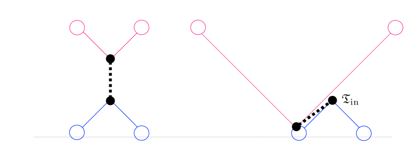
Figure 1: Schematic diagram in position space. Each of blue and red lines denotes the trajectory of the center of wave-packet for in and out states $\phi$, respectively. The thick dashed line denotes the trajectory of internal particle $\Phi$, while the black dots of its ends indicate that the interactions occur in a finite range with the spatial and time-like widths $\sim\sqrt{\sigma_{\text{in}}}$ and $\sqrt{\varsigma_{\text{in}}}$ ($\sim\sqrt{\sigma_{\text{out}}}$ and $\sqrt{\varsigma_{\text{out}}}$) around the point $\overline{\boldsymbol{\Xi}\!\left(\mathfrak{T}_{\text{in}}\right)}_{\text{in}}$ at time $\mathfrak{T}_{\text{in}}$ (point $\overline{\boldsymbol{\Xi}\!\left(\mathfrak{T}_{\text{out}}\right)}_{\text{out}}$ at time $\mathfrak{T}_{\text{out}}$), respectively. Circles are a reminder that each packet is given with a finite width, namely with the widths $\sim\sqrt{\sigma_{1}}$ and $\sqrt{\sigma_{2}}$ ($\sim\sqrt{\sigma_{3}}$ and $\sqrt{\sigma_{4}}$) at times $T_{1}$ and $T_{2}$ ($T_{3}$ and $T_{4}$) for the initial (final) wave packets. In the perturbation theory, we consider time evolution of the in-state from $T_{\text{in}}$ to $T_{\text{out}}$ in the interaction picture, which are chosen near $T_{1},T_{2}$ and $T_{3},T_{4}$, respectively, and the S-matrix element is taken with the out-state at $T_{\text{out}}$. The left figure shows an $s$-channel scattering without a backward propagation in the sense of the old-fashioned perturbation theory. The right figure explains that there always exists a final state configuration that realizes, e.g. $T_{1}\simeq\mathfrak{T}_{\text{out}}$ no matter how large we take a cluster-decomposition limit: $\left|\boldsymbol{\Xi}_{1}\!\left(T_{\text{in}}\right)-\boldsymbol{\Xi}_{2}\!\left(T_{\text{in}}\right)\right|\sim\left|\boldsymbol{X}_{1}-\boldsymbol{X}_{2}\right|\to\infty$.

We present and clarify two different interpretations of the result (56). We consider a finite time interval $T_{\text{out}}-T_{\text{in}}$. Without loss of generality, we focus on the initial time boundary at $T_{\text{in}}$ unless otherwise stated. First we stress that when we integrate over the final-state phase space $\boldsymbol{\Pi}_{3}$ and $\boldsymbol{\Pi}_{4}$ with varying interaction time $\mathfrak{T}_{\text{out}}$ ($=\Re\mathcal{T}_{\text{out}}$) accordingly to Eq. (54), there always exists a final-state configuration that gives a significant in-boundary effect at $T_{\text{in}}$, no matter what initial configuration we take, even a cluster-decomposition limit $\left|\boldsymbol{\Xi}_{1}\!\left(T_{\text{in}}\right)-\boldsymbol{\Xi}_{2}\!\left(T_{\text{in}}\right)\right|\to\infty$ and/or take $T_{\text{in}}\to-\infty$; see Fig. 1.

To illustrate qualitative behavior, let us tentatively focus on the expressions in the following limit [2]:

$$\left|\mathcal{T}-T_{\text{in}}\right| \gg{\sqrt{2\varsigma_{\text{out}}}},$$ (70)

which results in

$$G_{\text{out-int}}\!\left(\mathcal{T}\right) \to G_{\text{out-int}}^{\text{bulk}}\!\left(\mathcal{T}\right)-{1\over\sqrt{\pi}}e^{-{\left(\mathcal{T}-T_{\text{in}}\right)^{2}\over 2\varsigma_{\text{out}}}}{\sqrt{2\varsigma_{\text{out}}}\over\mathcal{T}-T_{\text{in}}}.$$ (71)

Note that the illustrative limit (70) implies that near the boundary, $\left(\Re\mathcal{T}_{\text{out}}-T_{\text{in}}\right)^{2}\lesssim 2\varsigma_{\text{out}}$, the deviation from the “energy conservation” is large:

$$\left(p^{0}-\mathcal{E}_{\text{out}}-\overline{\boldsymbol{V}}_{\text{out}}\cdot\boldsymbol{p}\right)^{2}=\left(\Im\mathcal{T}_{\text{out}}\right)^{2}\gg 2\varsigma_{\text{out}}.$$ (72)

From Eq. (71), we see that the boundary effect may become significant when $\mathcal{T}$ is near the in-boundary, namely when $\left(\Re\mathcal{T}-T_{\text{in}}\right)^{2}\lesssim 2\varsigma_{\text{out}}$ with $\left(\Im\mathcal{T}\right)\gg 2\varsigma_{\text{out}}$ as said above:

$$G_{\text{out-int}}\!\left(\mathcal{T}\right) \to-{1\over\sqrt{\pi}}e^{{\left(\Im\mathcal{T}\right)^{2}\over 2\varsigma_{\text{out}}}}{\sqrt{2\varsigma_{\text{out}}}\over i\,\Im\mathcal{T}}.$$ (73)

Note that the apparent exponential growth for the energy non-conserving limit $\left(\Im\mathcal{T}\right)^{2}\gg 2\varsigma_{\text{out}}$ is cancelled out by the existing energy conservation factor coming from

$$e^{-{\varsigma_{\text{out}}\over 2}\left(p^{0}-\mathcal{E}_{\text{out}}-\overline{\boldsymbol{V}}_{\text{out}}\cdot\boldsymbol{p}\right)^{2}} =e^{-{\left(\Im\mathcal{T}_{\text{out}}\right)^{2}\over 2\varsigma_{\text{out}}}}.$$ (74)

That is, the exponential suppression factor for a deviation from the energy conservation, $e^{-{\left(\Im\mathcal{T}_{\text{out}}\right)^{2}/2\varsigma_{\text{out}}}}$, is cencelled and replaced by the power suppression factor $1/\Im\mathcal{T}$ in the boundary effect. Recall that the boundary contribution from the configuration $\left(\Re{\mathcal{T}}_{\text{out}}-\mathfrak{T}_{\text{in}}\right)^{2}\lesssim 2\varsigma_{\text{out}}$ arises even if $\boldsymbol{X}_{3}$ and $\boldsymbol{X}_{4}$ are at a distance.

The existence of boundary effect crucially depends on the relation (28). The key question is the following: Can we well approximate the real physical setup in experiment, namely the Schrödinger-picture in-state $e^{-i\hat{H}t}\Ket{\text{in; }\Pi_{1}\Pi_{2}}$, by the “free Schrödinger-picture” state $e^{-i\hat{H}_{\text{free}}t}\Ket{\Pi_{1}\Pi_{2}}$, evolving in a virtual free world without any interaction, at $t=T_{\text{in}}$ when interactions are not negligible? If not, what state should we prepare for $e^{-i\hat{H}t}\Ket{\text{in; }\Pi_{1}\Pi_{2}}$ at $t=T_{\text{in}}$? Here we introduce two different constructions: “free” and “dressed”, which say yes and no for the first question, respectively.

3.1 Quantum mechanics basics

For the discussion below, let us recall the basics of quantum mechanics and spell out our notation. We identify the Schrödinger, Heisenberg, and interaction pictures at an arbitrary reference time $t_{\text{r}}$: For an arbitrary operator $\hat{O}$ in the Schrödinger picture, we relate them by

$$\hat{O}^{\text{I}}\!\left(t\right) =e^{i\hat{H}_{\text{free}}\,\left(t-t_{\text{r}}\right)}\hat{O}e^{-i\hat{H}_{\text{free}}\,\left(t-t_{\text{r}}\right)},$$ (75)

$$\hat{O}^{\text{H}}\!\left(t\right) =e^{i\hat{H}\,\left(t-t_{\text{r}}\right)}\hat{O}e^{-i\hat{H}\,\left(t-t_{\text{r}}\right)},$$ (76)

and for a time-independent state $\Ket{{\sf\Psi}}$ in the Heisenberg picture by

$$\Ket{{\sf\Psi};t}_{\text{I}} =e^{i\hat{H}_{\text{free}}\,\left(t-t_{\text{r}}\right)}e^{-i\hat{H}\,\left(t-t_{\text{r}}\right)}\Ket{{\sf\Psi}}$$

$$=\left(\operatorname{T}e^{-i\int_{t_{\text{r}}}^{t}\hat{H}_{\text{int}}^{\text{I}}\!\left(t^{\prime}-t_{\text{r}}\right)\,\text{d}t^{\prime}}\right)\Ket{{\sf\Psi}},$$ (77)

$$\Ket{{\sf\Psi};t}_{\text{S}} =e^{-i\hat{H}\,\left(t-t_{\text{r}}\right)}\Ket{{\sf\Psi}},$$ (78)

where we have used

$$\hat{U}\!\left(t_{1},t_{2}\right) :=e^{i\hat{H}_{\text{free}}\,\left(t_{1}-t_{\text{r}}\right)}e^{-i\hat{H}\,\left(t_{1}-t_{2}\right)}e^{-i\hat{H}_{\text{free}}\,\left(t_{2}-t_{\text{r}}\right)}$$

$$=\operatorname{T}e^{-i\int_{t_{2}-t_{\text{r}}}^{t_{1}-t_{\text{r}}}\hat{H}_{\text{int}}^{\text{I}}\!\left(t^{\prime}\right)\,\text{d}t^{\prime}}=\operatorname{T}e^{-i\int_{t_{2}}^{t_{1}}\hat{H}_{\text{int}}^{\text{I}}\!\left(t^{\prime}-t_{\text{r}}\right)\,\text{d}t^{\prime}}.$$ (79)

If an eigenbasis $\Ket{{\sf\Phi}}$ exist in the Schrödinger picture, $\hat{O}\Ket{{\sf\Phi}}=o\Ket{{\sf\Phi}}$, the corresponding operators in the interaction and Heisenberg pictures have the following eigenbases, respectively:

$$\Ket{{\sf\Phi};t}_{\text{IB}} =e^{i\hat{H}_{\text{free}}\,\left(t-t_{\text{r}}\right)}\Ket{{\sf\Phi}},$$ (80)

$$\Ket{{\sf\Phi};t}_{\text{HB}} =e^{i\hat{H}\,\left(t-t_{\text{r}}\right)}\Ket{{\sf\Phi}}.$$ (81)

The time dependence of these eigenbases is different from that of the states (77) and (78). Typically in our computation, $\hat{O}$ stands for $\hat{H}_{\text{free}}$.

3.2 “Free” construction

So far, we have chosen an arbitrary initial (final) time $T_{\text{in}}$ ($T_{\text{out}}$) anywhere near $T_{1}$ ($T_{3}$) and/or $T_{2}$ ($T_{4}$). In the “free” construction we identify the in and out Schrödinger-picture states at times $T_{\text{in}}$ and $T_{\text{out}}$, respectively, with a “free Schrödinger picture” state that evolves in a virtual free world governed by the free Hamiltonian no matter how significant interactions are at these times:

$$\Ket{\text{in; }\Pi_{1}\Pi_{2};t=T_{\text{in}}}_{\text{S}} =\Ket{\Pi_{1}\Pi_{2};t=T_{\text{in}}}_{\text{S}}^{\text{free}},$$

$$\Ket{\text{out; }\Pi_{3}\Pi_{4};t=T_{\text{out}}}_{\text{S}} =\Ket{\Pi_{3}\Pi_{4};t=T_{\text{out}}}_{\text{S}}^{\text{free}},$$ (82)

where we have defined the “free Schrödinger” state that evolves in the virtual free world:

$$\Ket{{\sf\Psi};t}_{\text{S}}^{\text{free}} :=e^{-i\hat{H}_{\text{free}}\,\left(t-t_{\text{r}}\right)}\Ket{{\sf\Psi}}.$$ (83)

In other words, the in and out states are given in the Heisenberg picture as

$$\Ket{\text{in; }\Pi_{1}\Pi_{2}} =e^{i\hat{H}\,\left(T_{\text{in}}-t_{\text{r}}\right)}e^{-i\hat{H}_{\text{free}}\,\left(T_{\text{in}}-t_{\text{r}}\right)}\Ket{\Pi_{1}\Pi_{2}},$$

$$\Ket{\text{out; }\Pi_{3}\Pi_{4}} =e^{i\hat{H}\,\left(T_{\text{out}}-t_{\text{r}}\right)}e^{-i\hat{H}_{\text{free}}\,\left(T_{\text{out}}-t_{\text{r}}\right)}\Ket{\Pi_{3}\Pi_{4}};$$ (84)

in the Schrödinger picture as

$$\Ket{\text{in; }\Pi_{1}\Pi_{2};t}_{\text{S}} =e^{-i\hat{H}\,\left(t-t_{\text{r}}\right)}\left(e^{i\hat{H}\,\left(T_{\text{in}}-t_{\text{r}}\right)}e^{-i\hat{H}_{\text{free}}\,\left(T_{\text{in}}-t_{\text{r}}\right)}\Ket{\Pi_{1}\Pi_{2}}\right)$$

$$=e^{-i\hat{H}\,\left(t-T_{\text{in}}\right)}e^{-i\hat{H}_{\text{free}}\,\left(T_{\text{in}}-t_{\text{r}}\right)}\Ket{\Pi_{1}\Pi_{2}},$$

$$\Ket{\text{out; }\Pi_{3}\Pi_{4};t}_{\text{S}} =e^{-i\hat{H}\,\left(t-t_{\text{r}}\right)}\left(e^{i\hat{H}\,\left(T_{\text{out}}-t_{\text{r}}\right)}e^{-i\hat{H}_{\text{free}}\,\left(T_{\text{out}}-t_{\text{r}}\right)}\Ket{\Pi_{3}\Pi_{4}}\right)$$

$$=e^{-i\hat{H}\,\left(t-T_{\text{out}}\right)}e^{-i\hat{H}_{\text{free}}\,\left(T_{\text{out}}-t_{\text{r}}\right)}\Ket{\Pi_{3}\Pi_{4}};$$ (85)

and in the interaction picture as

$$\Ket{\text{in; }\Pi_{1}\Pi_{2};t}_{\text{I}} =e^{i\hat{H}_{\text{free}}\,\left(t-t_{\text{r}}\right)}e^{-i\hat{H}\,\left(t-t_{\text{r}}\right)}\left(e^{i\hat{H}\,\left(T_{\text{in}}-t_{\text{r}}\right)}e^{-i\hat{H}_{\text{free}}\,\left(T_{\text{in}}-t_{\text{r}}\right)}\Ket{\Pi_{1}\Pi_{2}}\right)$$

$$=e^{i\hat{H}_{\text{free}}\,\left(t-t_{\text{r}}\right)}e^{-i\hat{H}\,\left(t-T_{\text{in}}\right)}e^{-i\hat{H}_{\text{free}}\,\left(T_{\text{in}}-t_{\text{r}}\right)}\Ket{\Pi_{1}\Pi_{2}}$$

$$=\operatorname{T}e^{-i\int_{T_{\text{in}}}^{t}\hat{H}_{\text{int}}^{\text{I}}\!\left(t^{\prime}-t_{\text{r}}\right)\,\text{d}t^{\prime}}\Ket{\Pi_{1}\Pi_{2}},$$

$$\Ket{\text{out; }\Pi_{3}\Pi_{4};t}_{\text{I}} =e^{i\hat{H}_{\text{free}}\,\left(t-t_{\text{r}}\right)}e^{-i\hat{H}\,\left(t-t_{\text{r}}\right)}\left(e^{i\hat{H}\,\left(T_{\text{out}}-t_{\text{r}}\right)}e^{-i\hat{H}_{\text{free}}\,\left(T_{\text{out}}-t_{\text{r}}\right)}\Ket{\Pi_{3}\Pi_{4}}\right)$$

$$=e^{i\hat{H}_{\text{free}}\,\left(t-t_{\text{r}}\right)}e^{-i\hat{H}\,\left(t-T_{\text{out}}\right)}e^{-i\hat{H}_{\text{free}}\,\left(T_{\text{out}}-t_{\text{r}}\right)}\Ket{\Pi_{3}\Pi_{4}}$$

$$=\operatorname{T}e^{-i\int_{T_{\text{out}}}^{t}\hat{H}_{\text{int}}^{\text{I}}\!\left(t^{\prime}-t_{\text{r}}\right)\,\text{d}t^{\prime}}\Ket{\Pi_{3}\Pi_{4}}.$$ (86)

One can trivially check the following:

$$\Ket{\text{in; }\Pi_{1}\Pi_{2}} =\Ket{\text{in; }\Pi_{1}\Pi_{2};t_{\text{r}}}_{\text{S}}=\Ket{\text{in; }\Pi_{1}\Pi_{2};t_{\text{r}}}_{\text{I}},$$

$$\Ket{\text{out; }\Pi_{3}\Pi_{4}} =\Ket{\text{out; }\Pi_{3}\Pi_{4};t_{\text{r}}}_{\text{S}}=\Ket{\text{out; }\Pi_{3}\Pi_{4};t_{\text{r}}}_{\text{I}}.$$ (87)

We also see that the Heisenberg-picture relation (84) reads in the Schrödinger picture,

$$\Ket{\text{in; }\Pi_{1}\Pi_{2};T_{\text{in}}}_{\text{S}} =e^{-i\hat{H}_{\text{free}}\,\left(T_{\text{in}}-t_{\text{r}}\right)}\Ket{\Pi_{1}\Pi_{2}},$$

$$\Ket{\text{out; }\Pi_{3}\Pi_{4};T_{\text{out}}}_{\text{S}} =e^{-i\hat{H}_{\text{free}}\,\left(T_{\text{out}}-t_{\text{r}}\right)}\Ket{\Pi_{3}\Pi_{4}},$$ (88)

and in the interaction picture,

$$\Ket{\text{in; }\Pi_{1}\Pi_{2};T_{\text{in}}}_{\text{I}} =\Ket{\Pi_{1}\Pi_{2}},$$

$$\Ket{\text{out; }\Pi_{3}\Pi_{4};T_{\text{out}}}_{\text{I}} =\Ket{\Pi_{3}\Pi_{4}}.$$ (89)

The “free” construction puts more emphasis on the interaction picture, in which the identification (89) appears most natural. We can also rewrite the probability amplitude as an inner product of the interaction-picture states at an arbitrary time $t$:

$$\mathcal{S} ={}_{\text{I}}\!\Braket{\text{out; }\Pi_{3}\Pi_{4};t}{\text{in; }\Pi_{1}\Pi_{2};t}_{\text{I}}$$

$$=\Bra{\Pi_{3}\Pi_{4}}\operatorname{T}e^{i\int^{t}_{T_{\text{out}}}\hat{H}_{\text{int}}^{\text{I}}\!\left(t^{\prime}-t_{\text{r}}\right)\,\text{d}t^{\prime}}e^{-i\int^{t}_{T_{\text{in}}}\hat{H}_{\text{int}}^{\text{I}}\!\left(t^{\prime}-t_{\text{r}}\right)\,\text{d}t^{\prime}}\Ket{\Pi_{1}\Pi_{2}}$$

$$=\Bra{\Pi_{3}\Pi_{4}}\operatorname{T}e^{-i\int^{T_{\text{out}}}_{T_{\text{in}}}\hat{H}_{\text{int}}^{\text{I}}\!\left(t^{\prime}-t_{\text{r}}\right)\,\text{d}t^{\prime}}\Ket{\Pi_{1}\Pi_{2}},$$ (90)

which becomes Eq. (36) when we set the arbitrary reference time $t_{\text{r}}=0$ as before. Note that the $t$ dependence drops out of the expression, and hence the probability does not depend on $t$.

We may say that the boundary effects remain even if the interaction is taken into account in the following sense [4] (see also Ref. [10]): Suppose that we transform the free states by a unitary operator $\hat{V}\!\left(\kappa\right)$ with $\hat{V}^{\dagger}\!\left(\kappa\right)\hat{V}\!\left(\kappa\right)=\hat{1}$ in Eq. (90):

$$\widetilde{\Ket{\Pi_{1}\Pi_{2}}} =\hat{V}\!\left(\kappa\right)\Ket{\Pi_{1}\Pi_{2}},$$ (91)

$$\widetilde{\Ket{\Pi_{3}\Pi_{4}}} =\hat{V}\!\left(\kappa\right)\Ket{\Pi_{3}\Pi_{4}}.$$ (92)

Then the S-matrix becomes

$$\widetilde{\mathcal{S}} =\widetilde{\Bra{\Pi_{3}\Pi_{4}}}\hat{U}\!\left(T_{\text{out}},T_{\text{in}}\right)\widetilde{\Ket{\Pi_{1}\Pi_{2}}}$$

$$=\Bra{\Pi_{3}\Pi_{4}}\hat{V}^{\dagger}\!\left(\kappa\right)\hat{U}\!\left(T_{\text{out}},T_{\text{in}}\right)\hat{V}\!\left(\kappa\right)\Ket{\Pi_{1}\Pi_{2}}.$$ (93)

If $\hat{V}$ is expanded as $\hat{V}=\hat{1}+\mathcal{O}\!\left(\kappa\right)$, we see from $\hat{U}\!\left(T_{\text{out}},T_{\text{in}}\right)=\hat{1}+\mathcal{O}\!\left(\kappa^{2}\right)$ that

$$\left[\hat{V}\!\left(\kappa\right),\hat{U}\!\left(T_{\text{out}},T_{\text{in}}\right)\right] =\mathcal{O}\!\left(\kappa^{3}\right),$$ (94)

and hence

$$\hat{V}^{\dagger}\!\left(\kappa\right)\hat{U}\!\left(T_{\text{out}},T_{\text{in}}\right)\hat{V}\!\left(\kappa\right) =\hat{U}\!\left(T_{\text{out}},T_{\text{in}}\right)+\mathcal{O}\!\left(\kappa^{3}\right).$$ (95)

Accordingly the order $\kappa^{2}$ contribution of the transition amplitudes are invariant under the unitary change of the free states.

3.3 “Dressed” construction

To repeat, we have chosen an arbitrary initial time $T_{\text{in}}$ anywhere near $T_{1}$ and/or $T_{2}$. One might feel it strange to identify the initial state as in Eq. (3.2) for a wave-packet configuration $\left(\boldsymbol{\Pi}_{1},\dots,\boldsymbol{\Pi}_{4}\right)$ that gives a significant overlap of the final-state wave-packets at $\mathfrak{T}_{\text{out}}\simeq T_{\text{in}}$ so that interactions are not negligible at $T_{\text{in}}$ as in the right panel in Fig. 1. In particular, the boundary interaction (71) crucially depends on the arbitrarily chosen $T_{\text{in}}$: For a given fixed initial and final state configuration $\left(\boldsymbol{\Pi}_{1},\dots,\boldsymbol{\Pi}_{4}\right)$, the boundary contribution drops off exponentially as we shift the arbitrarily chosen $T_{\text{in}}$ backwards in time.

The boundary effect is a consequence of the above-mentioned identification of the Heisenberg state $\Ket{\text{in; }\Pi_{1}\Pi_{2}}$ and $\Ket{\text{out; }\Pi_{3}\Pi_{4}}$ at $T_{\text{in}}$ and $T_{\text{out}}$, respectively. What if we identify different states at $T_{\text{in}}$ and $T_{\text{out}}$? Suppose that we take into account the interactions from $T_{\text{in}}^{\prime}$ $(<T_{\text{in}})$ to $T_{\text{in}}$ and from $T_{\text{out}}^{\prime}$ ($>T_{\text{out}}$) to $T_{\text{out}}$ (backward in time as $T_{\text{out}}<T_{\text{out}}^{\prime}$) in addition to the “free” construction above:

$$\Ket{\text{in; }\Pi_{1}\Pi_{2}}^{\prime} =e^{i\hat{H}\,\left(T_{\text{in}}-t_{\text{r}}\right)}e^{-i\hat{H}_{\text{free}}\,\left(T_{\text{in}}-t_{\text{r}}\right)}\operatorname{T}e^{-i\int_{T_{\text{in}}^{\prime}}^{T_{\text{in}}}\hat{H}_{\text{int}}\!\left(t^{\prime}-t_{\text{r}}\right)\,\text{d}t^{\prime}}\Ket{\Pi_{1}\Pi_{2}},$$

$$\Ket{\text{out; }\Pi_{3}\Pi_{4}}^{\prime} =e^{i\hat{H}\,\left(T_{\text{out}}-t_{\text{r}}\right)}e^{-i\hat{H}_{\text{free}}\,\left(T_{\text{out}}-t_{\text{r}}\right)}\operatorname{T}e^{-i\int^{T_{\text{out}}}_{T_{\text{out}}^{\prime}}\hat{H}_{\text{int}}\!\left(t^{\prime}-t_{\text{r}}\right)\,\text{d}t^{\prime}}\Ket{\Pi_{3}\Pi_{4}},$$ (96)

where we have replaced $\Ket{\Pi_{1}\Pi_{2}}$ and $\Ket{\Pi_{3}\Pi_{4}}$ in the “free” construction (84) by

$$\Ket{\Pi_{1}\Pi_{2}} \to\operatorname{T}e^{-i\int_{T_{\text{in}}^{\prime}}^{T_{\text{in}}}\hat{H}_{\text{int}}\!\left(t^{\prime}-t_{\text{r}}\right)\,\text{d}t^{\prime}}\Ket{\Pi_{1}\Pi_{2}},$$

$$\Ket{\Pi_{3}\Pi_{4}} \to\operatorname{T}e^{-i\int^{T_{\text{out}}}_{T_{\text{out}}^{\prime}}\hat{H}_{\text{int}}\!\left(t^{\prime}-t_{\text{r}}\right)\,\text{d}t^{\prime}}\Ket{\Pi_{3}\Pi_{4}}.$$ (97)

We note that the free basis $\Ket{\Pi_{1}\Pi_{2}}$ and the state $\operatorname{T}e^{-i\int_{T_{\text{in}}^{\prime}}^{T_{\text{in}}}\hat{H}_{\text{int}}\!\left(t^{\prime}-t_{\text{r}}\right)\,\text{d}t^{\prime}}\Ket{\Pi_{1}\Pi_{2}}$ are different from each other; the same note applies for the out ones. Note also that we can rewrite the Heisenberg-picture states (96) as

$$\Ket{\text{in; }\Pi_{1}\Pi_{2}}^{\prime} =e^{i\hat{H}\,\left(T_{\text{in}}-t_{\text{r}}\right)}e^{-i\hat{H}_{\text{free}}\,\left(T_{\text{in}}-t_{\text{r}}\right)}$$

$$\quad\times\left(e^{i\hat{H}_{\text{free}}\,\left(T_{\text{in}}-t_{\text{r}}\right)}e^{-i\hat{H}\,\left(T_{\text{in}}-t_{\text{r}}\right)}e^{i\hat{H}\left(T_{\text{in}}^{\prime}-t_{\text{r}}\right)}e^{-i\hat{H}_{\text{free}}\left(T_{\text{in}}^{\prime}-t_{\text{r}}\right)}\right)\Ket{\Pi_{1}\Pi_{2}}$$

$$=e^{i\hat{H}\left(T_{\text{in}}^{\prime}-t_{\text{r}}\right)}e^{-i\hat{H}_{\text{free}}\left(T_{\text{in}}^{\prime}-t_{\text{r}}\right)}\Ket{\Pi_{1}\Pi_{2}},$$

$$\Ket{\text{out; }\Pi_{3}\Pi_{4}}^{\prime} =e^{i\hat{H}\,\left(T_{\text{out}}-t_{\text{r}}\right)}e^{-i\hat{H}_{\text{free}}\,\left(T_{\text{out}}-t_{\text{r}}\right)}$$

$$\quad\times\left(e^{i\hat{H}_{\text{free}}\,\left(T_{\text{out}}-t_{\text{r}}\right)}e^{-i\hat{H}\,\left(T_{\text{out}}-t_{\text{r}}\right)}e^{i\hat{H}\left(t_{\text{out}}^{\prime}-t_{\text{r}}\right)}e^{-i\hat{H}_{\text{free}}\left(T_{\text{out}}^{\prime}-t_{\text{r}}\right)}\right)\Ket{\Pi_{1}\Pi_{2}}$$

$$=e^{i\hat{H}\left(T_{\text{out}}^{\prime}-t_{\text{r}}\right)}e^{-i\hat{H}_{\text{free}}\left(T_{\text{out}}^{\prime}-t_{\text{r}}\right)}\Ket{\Pi_{3}\Pi_{4}}.$$ (98)

In the Schrödinger picture, these are equivalent to

$$\Ket{\text{in; }\Pi_{1}\Pi_{2};t}^{\prime}_{\text{S}} =e^{-i\hat{H}\,\left(t-t_{\text{r}}\right)}\left(e^{i\hat{H}\left(T_{\text{in}}^{\prime}-t_{\text{r}}\right)}e^{-i\hat{H}_{\text{free}}\left(T_{\text{in}}^{\prime}-t_{\text{r}}\right)}\Ket{\Pi_{1}\Pi_{2}}\right)$$

$$=e^{-i\hat{H}\,\left(t-T_{\text{in}}^{\prime}\right)}e^{-i\hat{H}_{\text{free}}\,\left(T_{\text{in}}^{\prime}-t_{\text{r}}\right)}\Ket{\Pi_{1}\Pi_{2}},$$

$$\Ket{\text{out; }\Pi_{3}\Pi_{4};t}^{\prime}_{\text{S}} =e^{-i\hat{H}\,\left(t-t_{\text{r}}\right)}\left(e^{i\hat{H}\left(T_{\text{out}}^{\prime}-t_{\text{r}}\right)}e^{-i\hat{H}_{\text{free}}\left(T_{\text{out}}^{\prime}-t_{\text{r}}\right)}\Ket{\Pi_{3}\Pi_{4}}\right)$$

$$=e^{-i\hat{H}\,\left(t-T_{\text{out}}^{\prime}\right)}e^{-i\hat{H}_{\text{free}}\,\left(T_{\text{out}}^{\prime}-t_{\text{r}}\right)}\Ket{\Pi_{3}\Pi_{4}},$$ (99)

and in the interaction picture,

$$\Ket{\text{in; }\Pi_{1}\Pi_{2};t}^{\prime}_{\text{I}} =e^{i\hat{H}_{\text{free}}\,\left(t-t_{\text{r}}\right)}e^{-i\hat{H}\,\left(t-t_{\text{r}}\right)}\left(e^{i\hat{H}\left(T_{\text{in}}^{\prime}-t_{\text{r}}\right)}e^{-i\hat{H}_{\text{free}}\left(T_{\text{in}}^{\prime}-t_{\text{r}}\right)}\Ket{\Pi_{1}\Pi_{2}}\right)$$

$$=e^{i\hat{H}_{\text{free}}\,\left(t-t_{\text{r}}\right)}e^{-i\hat{H}\,\left(t-T_{\text{in}}^{\prime}\right)}e^{-i\hat{H}_{\text{free}}\left(T_{\text{in}}^{\prime}-t_{\text{r}}\right)}\Ket{\Pi_{1}\Pi_{2}}$$

$$=\operatorname{T}e^{-i\int_{T_{\text{in}}^{\prime}}^{t}\hat{H}^{\text{I}}_{\text{int}}\!\left(t^{\prime}-t_{\text{r}}\right)\,\text{d}t^{\prime}}\Ket{\Pi_{1}\Pi_{2}},$$ (100)

$$\Ket{\text{out; }\Pi_{3}\Pi_{3};t}^{\prime}_{\text{I}} =e^{i\hat{H}_{\text{free}}\,\left(t-t_{\text{r}}\right)}e^{-i\hat{H}\,\left(t-t_{\text{r}}\right)}\left(e^{i\hat{H}\left(T_{\text{out}}^{\prime}-t_{\text{r}}\right)}e^{-i\hat{H}_{\text{free}}\left(T_{\text{in}}^{\prime}-t_{\text{r}}\right)}\Ket{\Pi_{3}\Pi_{4}}\right)$$

$$=e^{i\hat{H}_{\text{free}}\,\left(t-t_{\text{r}}\right)}e^{-i\hat{H}\,\left(t-T_{\text{out}}^{\prime}\right)}e^{-i\hat{H}_{\text{free}}\left(T_{\text{out}}^{\prime}-t_{\text{r}}\right)}\Ket{\Pi_{3}\Pi_{4}}$$

$$=\operatorname{T}e^{-i\int_{T_{\text{out}}^{\prime}}^{t}\hat{H}^{\text{I}}_{\text{int}}\!\left(t^{\prime}-t_{\text{r}}\right)\,\text{d}t^{\prime}}\Ket{\Pi_{3}\Pi_{4}}.$$ (101)

Just as in the free construction (90), we may write the S-matrix as an inner product of the interaction-picture state at an arbitrary time $t$:

$$\mathcal{S}^{\prime} ={}^{\prime}_{\text{I}}\!\Braket{\text{out; }\Pi_{3}\Pi_{4};t}{\text{in; }\Pi_{1}\Pi_{2};t}_{\text{I}}^{\prime}$$

$$=\Bra{\Pi_{3}\Pi_{4}}\operatorname{T}e^{-i\int_{T_{\text{in}}^{\prime}}^{T_{\text{out}}^{\prime}}\hat{H}_{\text{int}}\!\left(t^{\prime}-t_{\text{r}}\right)\,\text{d}t^{\prime}}\Ket{\Pi_{1}\Pi_{2}},$$ (102)

from which the $t$-dependence drops out. Hereafter, we come back to the choice $t_{\text{r}}=0$. We note that $\mathcal{S}^{\prime}$ and $\mathcal{S}$ are physically different.

If we could take the limits $T_{\text{in}}^{\prime}\to-\infty$ and $T_{\text{out}}^{\prime}\to\infty$, we would be able to write

$$\mathcal{S}^{\prime} \to\Bra{\Pi_{3}\Pi_{4}}\operatorname{T}e^{-i\int_{-\infty}^{\infty}\hat{H}_{\text{int}}\!\left(t^{\prime}\right)\,\text{d}t^{\prime}}\Ket{\Pi_{1}\Pi_{2}}.$$ (103)

However, the limits

$$T_{\text{in}}^{\prime} \to-\infty, T_{\text{out}}^{\prime} \to\infty,$$ (104)

do not commute with the final-state integral of infinite volume over $\boldsymbol{\Pi}_{3}$ and $\boldsymbol{\Pi}_{4}$ as we will see below.

3.4 Comparison of two constructions

The in-boundary effect for the fixed configuration $\left(\boldsymbol{\Pi}_{1},\dots,\boldsymbol{\Pi}_{4}\right)$ disappears from $\mathcal{S}^{\prime}$, which includes the interaction from the time $T_{\text{in}}^{\prime}$ (or sufficiently earlier time than $T_{\text{in}}-\sqrt{2\varsigma_{\text{out}}}$ for the given final state configuration) to $T_{\text{in}}$ in Eq. (97). In the original $\mathcal{S}$ in the “free” construction, interactions at $t<T_{\text{in}}$ does not appear. If we start from $\mathcal{S}^{\prime}$ for the configuration $\left(\boldsymbol{\Pi}_{1},\dots,\boldsymbol{\Pi}_{4}\right)$, we recover the boundary effect of $\mathcal{S}$ by sharply switching off interactions at $t<T_{\text{in}}$.

Here in $\mathcal{S}^{\prime}$, although the free wave packets in $\Ket{\Pi_{1}\Pi_{2}}$ are given experimentally at $T_{1}$ and $T_{2}$, we identify $\Ket{\Pi_{1}\Pi_{2}}$ with the Heisenberg state at much earlier time $T_{\text{in}}^{\prime}$, not at somewhere $T_{\text{in}}$ near them. Namely, the Schrödinger-picture state $e^{-i\hat{H}t}\Ket{\text{in; }\Pi_{1}\Pi_{2}}^{\prime}$ at $t\to T_{\text{in}}^{\prime}$ is identified with the “free Schrödinger-picture” state $e^{-i\hat{H}_{\text{free}}t}\Ket{\Pi_{1}\Pi_{2}}$ that is time-evolved backward $t\to T_{\text{in}}^{\prime}$ in a virtual free world governed by $\hat{H}_{\text{free}}$, even for the case where interactions are not negligible for $t<T_{\text{in}}$. In $\Ket{\text{in; }\Pi_{1}\Pi_{2}}^{\prime}$, interactions are put at times much earlier than $T_{\text{in}}$ at which the supposedly free in-state is to be defined.

For the particular in and out-state configuration $\left(\boldsymbol{\Pi}_{1},\dots,\boldsymbol{\Pi}_{4}\right)$ with $\left(\mathfrak{T}_{\text{out}}-T_{\text{in}}\right)^{2}\lesssim 2\varsigma_{\text{out}}$, we may always choose $T_{\text{in}}^{\prime}\ll T_{\text{in}}-\sqrt{2\varsigma_{\text{out}}}$, and the in-boundary effect for this configuration drops out of $\mathcal{S}^{\prime}$, but there always exist other configuration $(\boldsymbol{\Pi}_{3},\boldsymbol{\Pi}_{4})$ that has the in-boundary effect at $\mathfrak{T}_{\text{out}}\simeq T_{\text{in}}^{\prime}$ accordingly to Eq. (54). Therefore, the probability summed over $(\boldsymbol{\Pi}_{3},\boldsymbol{\Pi}_{4})$ has the in-boundary effect for any fixed $T_{\text{in}}^{\prime}$.

Let us rephrase the above discussion in a slightly different way. As we move $T_{\text{in}}^{\prime}$ backwards, the bulk region expands, and the effective in-boundary at $T_{\text{in}}^{\prime}$ goes back in time. For a given $T_{\text{in}}^{\prime}$, the in-boundary contribution arises from the out state that has overlap of out wave packets at $T_{\text{in}}^{\prime}$. Therefore, the $T_{\text{in}}^{\prime}\to-\infty$ limit is not uniform because the region of in-boundary effect in $\boldsymbol{\Pi}_{3}\boldsymbol{\Pi}_{4}$ moves along with $T_{\text{in}}^{\prime}$. For these out states for given $T_{\text{in}}^{\prime}$, the boundary effect persists. If such an out state is not included, the boundary effect disappears.

To summarize so far, for any configuration of $\boldsymbol{\Pi}_{3}$ and $\boldsymbol{\Pi}_{4}$, there always exists a $T_{\text{in}}^{\prime}$ that removes the boundary effect, while for any $T_{\text{in}}^{\prime}$, there always exists a configuration of $\boldsymbol{\Pi}_{3}$ and $\boldsymbol{\Pi}_{4}$ that yields an in-boundary effect. Therefore it is subject to debate whether or not the limit (104) can be taken to remove all the time boundary effects.

The expression for boundary effect in the second term in Eq. (71) vanishes exponentially in the limit $T_{\text{in}}\to-\infty$. In the “dressed” construction, this is natural because this limit corresponds to taking into account all the interactions from $-\infty$, for the fixed initial and final state configurations. In the “free” construction, one emphasizes the fact that no matter how much we take the limit $T_{\text{in}}\to-\infty$, there always exists a final state configuration with $\left(\Re\mathcal{T}_{\text{out}}-T_{\text{in}}\right)^{2}\lesssim 2\varsigma_{\text{out}}$ for a given $T_{\text{in}}$. The difference of two constructions is the order of procedures: taking the limit $T_{\text{in}}\to\infty$ first vs integrating over the infinite volume of $\left(\boldsymbol{\Pi}_{3},\boldsymbol{\Pi}_{4}\right)$ first.

So far, both constructions have pros and cons, subject to one’s theoretical prejudice. Ultimately, experiment should determine which (or else) is right. Currently, an experiment is on-going [11] based on the “free” construction [12]. In this paper, we will leave the choice of constructions open, and concentrate on the wave effect that persists even when we only take into account the bulk effects. See Sec. 4.2 for related discussion on the in-boundary effect for $1\to 2$ decay of $\Phi\to\phi\phi$.

4 Bulk amplitude

Hereafter, we focus on the bulk contribution and do not take the boundary contributions into account. We will perform the integration of the virtual momentum $p$ of $\Phi$ in the saddle-point approximation. Note that so far the Gaussian integral over the position of interaction $x$ and $x^{\prime}$ is exact, up to the time-boundary effects for $t=x^{0}$ and $t^{\prime}=x^{\prime 0}$.

4.1 Bulk amplitude after integral over internal momentum

Neglecting the time-boundary contribution, the probability amplitude in Eq. (56) becomes

$$\mathcal{S} =i\kappa^{2}\left(\prod_{A=1}^{4}{1\over\sqrt{2E_{A}}}\left(1\over\pi\sigma_{A}\right)^{3/4}\right)\left(2\pi\sigma_{\text{in}}\right)^{3/2}\left(2\pi\sigma_{\text{out}}\right)^{3/2}\sqrt{2\pi\varsigma_{\text{in}}}\sqrt{2\pi\varsigma_{\text{out}}}\int{\text{d}^{4}p\over\left(2\pi\right)^{4}}{1\over p^{2}+M^{2}-i\epsilon}$$

$$\quad\times e^{-{\sigma_{\text{out}}\over 2}\left(\boldsymbol{p}-\boldsymbol{P}_{\text{out}}\right)^{2}-{\mathcal{R}_{\text{out}}\over 2}+i\overline{\boldsymbol{\mathfrak{X}}}_{\text{out}}\cdot\left(\boldsymbol{p}-\boldsymbol{P}_{\text{out}}\right)-i\mathfrak{T}_{\text{out}}\left(p^{0}-\mathcal{E}_{\text{out}}-\overline{\boldsymbol{V}}_{\text{out}}\cdot\boldsymbol{p}\right)-{\varsigma_{\text{out}}\over 2}\left(p^{0}-\mathcal{E}_{\text{out}}-\overline{\boldsymbol{V}}_{\text{out}}\cdot\boldsymbol{p}\right)^{2}}$$

$$\quad\times e^{-{\sigma_{\text{in}}\over 2}\left(\boldsymbol{p}-\boldsymbol{P}_{\text{in}}\right)^{2}-{\mathcal{R}_{\text{in}}\over 2}-i\overline{\boldsymbol{\mathfrak{X}}}_{\text{in}}\cdot\left(\boldsymbol{p}-\boldsymbol{P}_{\text{in}}\right)+i\mathfrak{T}_{\text{in}}\left(p^{0}-\mathcal{E}_{\text{in}}-\overline{\boldsymbol{V}}_{\text{in}}\cdot\boldsymbol{p}\right)-{\varsigma_{\text{in}}\over 2}\left(p^{0}-\mathcal{E}_{\text{in}}-\overline{\boldsymbol{V}}_{\text{in}}\cdot\boldsymbol{p}\right)^{2}}.$$ (105)

We can square-complete the $p^{0}$-dependent four terms in the above exponent as

$$-{\varsigma_{+}\over 2}\left(p^{0}-\Omega\!\left(\boldsymbol{p}\right)+i{\delta\mathfrak{T}\over\varsigma_{+}}\right)^{2}-{\varsigma\over 2}\bigl{(}\omega_{\text{out}}\!\left(\boldsymbol{p}\right)-\omega_{\text{in}}\!\left(\boldsymbol{p}\right)\bigr{)}^{2}-{\left(\delta\mathfrak{T}\right)^{2}\over 2\varsigma_{+}}$$

$$+i\varsigma\left({\mathfrak{T}_{\text{in}}\over\varsigma_{\text{in}}}+{\mathfrak{T}_{\text{out}}\over\varsigma_{\text{out}}}\right)\left(\omega_{\text{out}}\!\left(\boldsymbol{p}\right)-\omega_{\text{in}}\!\left(\boldsymbol{p}\right)\right)$$ (106)

where we have defined

$$\varsigma_{+} :=\varsigma_{\text{in}}+\varsigma_{\text{out}},$$

$$\varsigma :=\left({1\over\varsigma_{\text{in}}}+{1\over\varsigma_{\text{out}}}\right)^{-1},$$

$$\delta\mathfrak{T} :=\mathfrak{T}_{\text{out}}-\mathfrak{T}_{\text{in}},$$

$$\omega_{\text{in}}\!\left(\boldsymbol{p}\right) :=\mathcal{E}_{\text{in}}+\overline{\boldsymbol{V}}_{\text{in}}\cdot\boldsymbol{p},$$

$$\omega_{\text{out}}\!\left(\boldsymbol{p}\right) :=\mathcal{E}_{\text{out}}+\overline{\boldsymbol{V}}_{\text{out}}\cdot\boldsymbol{p},$$ (107)

and the typical “average energy” for the $2\to 2$ process

$$\Omega\!\left(\boldsymbol{p}\right) :={\varsigma_{\text{in}}\omega_{\text{in}}\!\left(\boldsymbol{p}\right)+\varsigma_{\text{out}}\omega_{\text{out}}\!\left(\boldsymbol{p}\right)\over\varsigma_{\text{in}}+\varsigma_{\text{out}}}.$$ (108)

By the saddle-point approximation, we get

$$\mathcal{S} =i\kappa^{2}\left(\prod_{A=1}^{4}{1\over\sqrt{2E_{A}}}\left(1\over\pi\sigma_{A}\right)^{3/4}\right)\left(2\pi\sigma_{\text{in}}\right)^{3/2}\left(2\pi\sigma_{\text{out}}\right)^{3/2}\sqrt{2\pi\varsigma}$$

$$\quad\times\int{\text{d}^{3}\boldsymbol{p}\over\left(2\pi\right)^{3}}{1\over-\left(\Omega\!\left(\boldsymbol{p}\right)-{i\,\delta\mathfrak{T}\over\varsigma_{+}}\right)^{2}+\boldsymbol{p}^{2}+M^{2}-i\epsilon}$$

$$\quad\times e^{-{\sigma_{\text{out}}\over 2}\left(\boldsymbol{p}-\boldsymbol{P}_{\text{out}}\right)^{2}-{\mathcal{R}_{\text{out}}\over 2}+i\overline{\boldsymbol{\mathfrak{X}}}_{\text{out}}\cdot\left(\boldsymbol{p}-\boldsymbol{P}_{\text{out}}\right)-{\sigma_{\text{in}}\over 2}\left(\boldsymbol{p}-\boldsymbol{P}_{\text{in}}\right)^{2}-{\mathcal{R}_{\text{in}}\over 2}-i\overline{\boldsymbol{\mathfrak{X}}}_{\text{in}}\cdot\left(\boldsymbol{p}-\boldsymbol{P}_{\text{in}}\right)}$$

$$\quad\times e^{-{\varsigma\over 2}\bigl{(}\omega_{\text{out}}\!\left(\boldsymbol{p}\right)-\omega_{\text{in}}\!\left(\boldsymbol{p}\right)\bigr{)}^{2}-i\Omega\!\left(\boldsymbol{p}\right)\delta\mathfrak{T}-{\left(\delta\mathfrak{T}\right)^{2}\over 2\varsigma_{+}}+i\left(\omega_{\text{out}}\!\left(\boldsymbol{p}\right)\mathfrak{T}_{\text{out}}-\omega_{\text{in}}\!\left(\boldsymbol{p}\right)\mathfrak{T}_{\text{in}}\right)}.$$ (109)

Here, the $\boldsymbol{p}$ dependence of the exponent $e^{\widetilde{F}}$ is of the form

$$\widetilde{F} =-{\sigma_{+}\over 2}\boldsymbol{p}^{2}-{\varsigma\over 2}\left(\delta\overline{\boldsymbol{V}}\cdot\boldsymbol{p}\right)^{2}+\boldsymbol{w}\cdot\boldsymbol{p}+C,$$ (110)

where

$$\sigma_{+} :=\sigma_{\text{in}}+\sigma_{\text{out}},$$ (111)

$$\delta\overline{\boldsymbol{V}} :=\overline{\boldsymbol{V}}_{\text{out}}-\overline{\boldsymbol{V}}_{\text{in}},$$ (112)

$$\boldsymbol{w} :=\sigma_{+}\boldsymbol{\mathcal{P}}-\varsigma\,\delta\mathcal{E}\,\delta\overline{\boldsymbol{V}}+i\left(\delta\overline{\boldsymbol{\mathfrak{X}}}+\mathfrak{T}_{\varsigma}\,\delta\overline{\boldsymbol{V}}\right),$$ (113)

$$C :=-{\sigma_{\text{in}}\over 2}\boldsymbol{P}_{\text{in}}^{2}-{\sigma_{\text{out}}\over 2}\boldsymbol{P}_{\text{out}}^{2}-{\mathcal{R}_{\text{in}}+\mathcal{R}_{\text{out}}\over 2}-{\varsigma\over 2}\left(\delta\mathcal{E}\right)^{2}-{\left(\delta\mathfrak{T}\right)^{2}\over 2\varsigma_{+}}$$

$$\quad+i\left[\overline{\boldsymbol{\mathfrak{X}}}_{\text{in}}\cdot\boldsymbol{P}_{\text{in}}-\overline{\boldsymbol{\mathfrak{X}}}_{\text{out}}\cdot\boldsymbol{P}_{\text{out}}+\mathfrak{T}_{\varsigma}\delta\mathcal{E}\right],$$ (114)

in which

$$\delta\mathfrak{T} :=\mathfrak{T}_{\text{out}}-\mathfrak{T}_{\text{in}},$$ (115)

$$\delta\overline{\boldsymbol{\mathfrak{X}}} :=\overline{\boldsymbol{\mathfrak{X}}}_{\text{out}}-\overline{\boldsymbol{\mathfrak{X}}}_{\text{in}},$$ (116)

$$\delta\mathcal{E} :=\mathcal{E}_{\text{out}}-\mathcal{E}_{\text{in}},$$ (117)

and we have defined the “average momentum” for the $2\to 2$ process

$$\boldsymbol{\mathcal{P}} :={\sigma_{\text{in}}\boldsymbol{P}_{\text{in}}+\sigma_{\text{out}}\boldsymbol{P}_{\text{out}}\over\sigma_{\text{in}}+\sigma_{\text{out}}}$$ (118)

and the “interaction time” for the $2\to 2$ process

$$\mathfrak{T}_{\varsigma} :=\varsigma\left({\mathfrak{T}_{\text{in}}\over\varsigma_{\text{in}}}+{\mathfrak{T}_{\text{out}}\over\varsigma_{\text{out}}}\right).$$ (119)

Note that the last term in Eq. (4.1) (in its second line) can be dropped out since it is a pure imaginary constant.

The saddle point ${\partial\widetilde{F}\over\partial p_{i}}=0$ is at

$$p_{*i} ={w_{i}\over\sigma_{+}}-{\varsigma\left(\delta\overline{\boldsymbol{V}}\right)_{i}\left(\delta\overline{\boldsymbol{V}}\cdot\boldsymbol{w}\right)\over\sigma_{+}\left(\sigma_{+}+\varsigma\left(\delta\overline{\boldsymbol{V}}\right)^{2}\right)},$$ (120)

that is,

$$\boldsymbol{p}_{*} =\left(\boldsymbol{\mathcal{P}}-{\varsigma\,\delta\mathcal{E}\,\delta\overline{\boldsymbol{V}}-i\left(\delta\overline{\boldsymbol{\mathfrak{X}}}+\mathfrak{T}_{\varsigma}\,\delta\overline{\boldsymbol{V}}\right)\over\sigma_{+}}\right)-{\varsigma\left(\delta\overline{\boldsymbol{V}}\right)^{2}\over\sigma_{+}+\varsigma\left(\delta\overline{\boldsymbol{V}}\right)^{2}}\left(\boldsymbol{\mathcal{P}}-{\varsigma\,\delta\mathcal{E}\,\delta\overline{\boldsymbol{V}}-i\left(\delta\overline{\boldsymbol{\mathfrak{X}}}+\mathfrak{T}_{\varsigma}\,\delta\overline{\boldsymbol{V}}\right)\over\sigma_{+}}\right)_{\parallel}$$ (121)

where

$$\boldsymbol{Q}_{\parallel} ={\left(\delta\overline{\boldsymbol{V}}\cdot\boldsymbol{Q}\right)\over\left(\delta\overline{\boldsymbol{V}}\right)^{2}}\delta\overline{\boldsymbol{V}}.$$ (122)

Now we can rewrite $\widetilde{F}$ without any approximation as

$$\widetilde{F} =-{1\over 2}\left(\boldsymbol{p}-\boldsymbol{p}_{*}\right)_{i}\left(\sigma_{+}\delta_{ij}+\varsigma\left(\delta\overline{\boldsymbol{V}}\right)_{i}\left(\delta\overline{\boldsymbol{V}}\right)_{j}\right)\left(\boldsymbol{p}-\boldsymbol{p}_{*}\right)_{j}+\widetilde{F}_{*},$$ (123)

where

$$\widetilde{F}_{*} ={1\over 2\sigma_{+}}\left(\boldsymbol{w}^{2}-{\varsigma\left(\delta\overline{\boldsymbol{V}}\cdot\boldsymbol{w}\right)^{2}\over\sigma_{+}+\varsigma\left(\delta\overline{\boldsymbol{V}}\right)^{2}}\right)+C.$$ (124)

Let us separate two terms corresponding to the momentum and energy conservation from $\widetilde{F}_{*}$:

$$\widetilde{F}_{*} =F_{*}-{\sigma\over 2}\left(\delta\boldsymbol{P}\right)^{2}-{\varsigma\sigma_{+}\over 2\left(\sigma_{+}+\varsigma\left(\delta\overline{\boldsymbol{V}}\right)^{2}\right)}\left(\delta E-\boldsymbol{V}_{\sigma}\cdot\delta\boldsymbol{P}\right)^{2},$$ (125)

where we have defined

$$\sigma :=\left({1\over\sigma_{\text{in}}}+{1\over\sigma_{\text{out}}}\right)^{-1}=\left(\sum_{a=1}^{4}{1\over\sigma_{a}}\right)^{-1},$$ (126)

$$\delta E :=E_{\text{out}}-E_{\text{in}},$$ (127)

$$\delta\boldsymbol{P} :=\boldsymbol{P}_{\text{out}}-\boldsymbol{P}_{\text{in}},$$ (128)

$$F_{*} :=-{\mathcal{R}_{\text{in}}+\mathcal{R}_{\text{out}}\over 2}-{\left(\delta\mathfrak{T}\right)^{2}\over 2\varsigma_{+}}$$

$$\phantom{:=\,\,}-{\varsigma\over 2\left(\sigma_{+}+\varsigma\left(\delta\overline{\boldsymbol{V}}\right)^{2}\right)}\left({\left(\delta\overline{\boldsymbol{V}}\right)^{2}\left(\delta\overline{\boldsymbol{\mathfrak{X}}}\right)^{2}-\left(\delta\overline{\boldsymbol{V}}\cdot\delta\overline{\boldsymbol{\mathfrak{X}}}\right)^{2}\over\sigma_{+}}+{\left(\delta\overline{\boldsymbol{\mathfrak{X}}}+\mathfrak{T}_{\varsigma}\delta\overline{\boldsymbol{V}}\right)^{2}\over\varsigma}\right),$$ (129)

and the “average velocity” for the $2\to 2$ process

$$\boldsymbol{V}_{\sigma} :=\sigma\left({\overline{\boldsymbol{V}}_{\text{in}}\over\sigma_{\text{in}}}+{\overline{\boldsymbol{V}}_{\text{out}}\over\sigma_{\text{out}}}\right),$$ (130)

and have used the identity

$$\delta\mathcal{E}+\delta\overline{\boldsymbol{V}}\cdot\boldsymbol{\mathcal{P}}=\delta E-\boldsymbol{V}_{\sigma}\cdot\delta\boldsymbol{P}.$$ (131)

We see from the first term in the parentheses in Eq. (129) that the suppression is weaker when the “impact parameter” $\delta\overline{\boldsymbol{\mathfrak{X}}}$ is parallel to the “momentum transfer” $\delta\overline{\boldsymbol{V}}$. This combination $\left(\delta\overline{\boldsymbol{V}}\right)^{2}\left(\delta\overline{\boldsymbol{\mathfrak{X}}}\right)^{2}-\left(\delta\overline{\boldsymbol{V}}\cdot\delta\overline{\boldsymbol{\mathfrak{X}}}\right)^{2}$ is always non-negative due to the Cauchy-Schwarz inequality. Also from the second term, the suppression is weaker when the difference of the average position of in and out states is close at the “$2\to 2$ interaction time” $\mathfrak{T}_{\varsigma}$, namely when $\left|\delta\overline{\boldsymbol{\mathfrak{X}}}+\mathfrak{T}_{\varsigma}\delta\overline{\boldsymbol{V}}\right|$ is small.

For the integrating over $\boldsymbol{p}$, the Gaussian factor is

$$\sqrt{\left(2\pi\right)^{3}\over\sigma_{+}^{2}\left(\sigma_{+}+\varsigma\left(\delta\overline{\boldsymbol{V}}\right)^{2}\right)}.$$ (132)

Finally we get the differential amplitude for a fixed configuration of initial and final states $\left(\boldsymbol{\Pi}_{1},\dots,\boldsymbol{\Pi}_{4}\right)$:

$$\mathcal{S} =i\mathcal{M}\left(\prod_{A=1}^{4}{1\over\sqrt{2E_{A}}}\left(1\over\pi\sigma_{A}\right)^{3/4}\right)$$

$$\quad\times\left(2\pi\right)^{4}\left[\left(\sigma\over 2\pi\right)^{3/2}e^{-{\sigma\over 2}\left(\delta\boldsymbol{P}\right)^{2}}\right]\left[\left({1\over 2\pi}{\varsigma\sigma_{+}\over\sigma_{+}+\varsigma\left(\delta\overline{\boldsymbol{V}}\right)^{2}}\right)^{1/2}e^{-{1\over 2}{\varsigma\sigma_{+}\over\sigma_{+}+\varsigma\left(\delta\overline{\boldsymbol{V}}\right)^{2}}\left(\delta E-\boldsymbol{V}_{\sigma}\cdot\delta\boldsymbol{P}\right)^{2}}\right],$$ (133)

where we have defined the dimensionless amplitude $\mathcal{M}$; cf. Eq. (188):

$$\mathcal{M} :={\kappa^{2}e^{F_{*}}\over-\left(\left(\Omega\!\left(\boldsymbol{p}_{*}\right)\right)^{2}-\left(\delta\mathfrak{T}\over\varsigma_{+}\right)^{2}\right)+i2\Omega\!\left(\boldsymbol{p}_{*}\right){\delta\mathfrak{T}\over\varsigma_{+}}+\boldsymbol{p}_{*}^{2}+M^{2}-i\epsilon}$$

$$={\kappa^{2}\over-\left(\left(\Omega\!\left(\boldsymbol{p}_{*}\right)\right)^{2}-\left(\delta\mathfrak{T}\over\varsigma_{+}\right)^{2}\right)+i2\Omega\!\left(\boldsymbol{p}_{*}\right){\delta\mathfrak{T}\over\varsigma_{+}}+\boldsymbol{p}_{*}^{2}+M^{2}-i\epsilon}$$

$$\quad\times e^{-{\mathcal{R}_{\text{in}}+\mathcal{R}_{\text{out}}\over 2}-{\left(\delta\mathfrak{T}\right)^{2}\over 2\varsigma_{+}}-{\varsigma\over 2\left(\sigma_{+}+\varsigma\left(\delta\overline{\boldsymbol{V}}\right)^{2}\right)}\left({\left(\delta\overline{\boldsymbol{V}}\right)^{2}\left(\delta\overline{\boldsymbol{\mathfrak{X}}}\right)^{2}-\left(\delta\overline{\boldsymbol{V}}\cdot\delta\overline{\boldsymbol{\mathfrak{X}}}\right)^{2}\over\sigma_{+}}+{\left(\delta\overline{\boldsymbol{\mathfrak{X}}}+\mathfrak{T}_{\varsigma}\delta\overline{\boldsymbol{V}}\right)^{2}\over\varsigma}\right)}.$$ (134)

Several comments are in order:

• All the terms in $F_{*}$ are negative or zero, and hence $F_{*}$ gives always a suppression factor.

• In the amplitude (133), the plane-wave limit $\sigma\to\infty$ gives a delta function for the momentum conservation:

  $$\left(\sigma\over 2\pi\right)^{3/2}e^{-{\sigma\over 2}\left(\delta\boldsymbol{P}\right)^{2}} \to\delta^{3}\!\left(\delta\boldsymbol{P}\right)=\delta^{3}\!\bigl{(}\boldsymbol{P}_{\text{out}}-\boldsymbol{P}_{\text{in}}\bigr{)}.$$ (135)

• Likewise, the limit ${\varsigma\sigma_{+}\over\sigma_{+}+\varsigma\left(\delta\overline{\boldsymbol{V}}\right)^{2}}\to\infty$ gives a delta function for the energy conservation:

  $$\left({1\over 2\pi}{\varsigma\sigma_{+}\over\sigma_{+}+\varsigma\left(\delta\overline{\boldsymbol{V}}\right)^{2}}\right)^{1/2}e^{-{1\over 2}{\varsigma\sigma_{+}\over\sigma_{+}+\varsigma\left(\delta\overline{\boldsymbol{V}}\right)^{2}}\left(\delta E-\boldsymbol{V}_{\sigma}\cdot\delta\boldsymbol{P}\right)^{2}} \to\delta\!\left(\delta E-\boldsymbol{V}_{\sigma}\cdot\delta\boldsymbol{P}\right).$$ (136)

• In the squared amplitude $\left|\mathcal{S}\right|^{2}$, the factor $e^{-\sigma\left(\delta\boldsymbol{P}\right)^{2}}$ gives the momentum conservation in the limit $\sigma\to\infty$:

  $$\left(\sigma\over\pi\right)^{3/2}e^{-\sigma\left(\delta\boldsymbol{P}\right)^{2}} \to\delta^{3}\bigl{(}\boldsymbol{P}_{\text{out}}-\boldsymbol{P}_{\text{in}}\bigr{)}.$$ (137)

  We note that the infinity $\delta^{3}\!\left(0\right)$ from $\left[\delta^{3}\bigl{(}\delta\boldsymbol{P}\bigr{)}\right]^{2}$ that appears in the plane-wave computation, using the right-hand side in Eq. (135), is tamed in the current wave-packet one: The would-be delta function squared becomes another would-be delta function again.

• Likewise, the factor

  $$\exp\!\left(-{\varsigma\sigma_{+}\over\sigma_{+}+\varsigma\left(\delta\overline{\boldsymbol{V}}\right)^{2}}\left(\delta E-\boldsymbol{V}_{\sigma}\cdot\delta\boldsymbol{P}\right)^{2}\right)$$

  in $\left|\mathcal{S}\right|^{2}$ gives the energy conservation in the limit ${\varsigma\sigma_{+}\over\sigma_{+}+\varsigma\left(\delta\overline{\boldsymbol{V}}\right)^{2}}\to\infty$:

  $$\sqrt{{1\over\pi}{\varsigma\sigma_{+}\over\sigma_{+}+\varsigma\left(\delta\overline{\boldsymbol{V}}\right)^{2}}}\,e^{-{\varsigma\sigma_{+}\over\sigma_{+}+\varsigma\left(\delta\overline{\boldsymbol{V}}\right)^{2}}\left(\delta E-\boldsymbol{V}_{\sigma}\cdot\delta\boldsymbol{P}\right)^{2}} \to\delta\bigl{(}E_{\text{out}}-E_{\text{in}}-\boldsymbol{V}_{\sigma}\cdot\left(\boldsymbol{P}_{\text{out}}-\boldsymbol{P}_{\text{in}}\right)\bigr{)}.$$ (138)

  Note that the energy conservation is deformed by the wave-packet effect $\boldsymbol{V}_{\sigma}\cdot\delta\boldsymbol{P}$, which goes to zero in the momentum conserving limit: $\delta\boldsymbol{P}\to 0$.

• It is remarkable that the wave effect persists even without the time-boundary effect. Namely, the real and imaginary parts of the pole of propagator are shifted as in Eq. (134). Even when $\boldsymbol{p}_{*}\simeq P_{\text{in}}$ and $\Omega\!\left(\boldsymbol{p}_{*}\right)\simeq E_{\text{in}}$, the pole position of the propagator is shifted such that the mass-squared $M^{2}$ and decay width $\Gamma$ are shifted by $\left(\delta\mathfrak{T}/\varsigma_{+}\right)^{2}$ and $-2E_{\text{in}}\delta\mathfrak{T}/\varsigma_{+}M$, respectively.

4.2 In-boundary effect for decay

Here we discuss how our result for the $2\to 2$ scattering $\phi\phi\to\Phi\to\phi\phi$ can be applied to the $1\to 2$ decay process $\Phi\to\phi\phi$. In Sec. 3, we have presented two different constructions regarding the boundary effect. For the $1\to 2$ decay $\Phi\to\phi\phi$ [2], the key question for its in-boundary effect is how we can better take into account the production process of $\Phi$. Which approximates an experimentally prepared state of $\Phi$ better at an initial time $T_{\text{in}}^{\text{decay}}$? Is it the Heisenberg state

$$\Ket{\text{in; }\Phi}=e^{i\hat{H}T_{\text{in}}^{\text{decay}}}e^{-i\hat{H}_{\text{free}}T_{\text{in}}^{\text{decay}}}\Ket{\Phi}$$ (139)

in the free construction, or

$$\Ket{\text{in; }\Phi}^{\prime} =e^{i\hat{H}T_{\text{in}}^{\text{decay}}}e^{-i\hat{H}_{\text{free}}T_{\text{in}}^{\text{decay}}}\operatorname{T}e^{-i\int_{T^{\prime}}^{T_{\text{in}}^{\text{decay}}}H^{\text{I}}_{\text{int}}\!\left(t^{\prime}\right)\,\text{d}t^{\prime}}\Ket{\Phi} (T^{\prime}\to-\infty)$$ (140)

in the dressed construction?

In our result for the $2\to 2$ $s$-channel scattering of $\phi\phi\to\Phi\to\phi\phi$, the interaction time $\mathfrak{T}_{\text{in}}$ would correspond to $T_{\text{in}}^{\text{decay}}$ for the $\Phi\to\phi\phi$ decay. Here we note that the in-boundary effect of the decay becomes significant when the decay-interaction point around $\mathfrak{T}_{\text{out}}$ is near the center of the in-state wave packet at $T_{\text{in}}^{\text{decay}}\simeq\mathfrak{T}_{\text{in}}$, namely when

$$\left(\delta\mathfrak{T}\right)^{2}=\left(\mathfrak{T}_{\text{out}}-\mathfrak{T}_{\text{in}}\right)^{2}\lesssim 2\varsigma_{\text{out}}.$$ (141)

Therefore, one might interpret that the limit $\delta\mathfrak{T}\to 0$, which necessarily arises when we integrate over the final state phase space $\boldsymbol{\Pi}_{3}$ and $\boldsymbol{\Pi}_{4}$, corresponds to the in-boundary for the $1\to 2$ decay. By taking $\delta\mathfrak{T}\to 0$ in Eq. (134), we obtain

$$\mathcal{M} \to{\kappa^{2}\over-\bigl{(}\Omega\!\left(\boldsymbol{p}_{*}\right)\bigr{)}^{2}+\boldsymbol{p}_{*}^{2}+M^{2}-i\epsilon}$$

$$\quad\times e^{-{\mathcal{R}_{\text{in}}+\mathcal{R}_{\text{out}}\over 2}-{\varsigma\over 2\left(\sigma_{+}+\varsigma\left(\delta\overline{\boldsymbol{V}}\right)^{2}\right)}\left({\left(\delta\overline{\boldsymbol{V}}\right)^{2}\left(\delta\overline{\boldsymbol{\mathfrak{X}}}\right)^{2}-\left(\delta\overline{\boldsymbol{V}}\cdot\delta\overline{\boldsymbol{\mathfrak{X}}}\right)^{2}\over\sigma_{+}}+{\left(\delta\overline{\boldsymbol{\mathfrak{X}}}+\mathfrak{T}_{\varsigma}\delta\overline{\boldsymbol{V}}\right)^{2}\over\varsigma}\right)}.$$ (142)

We see that there is no $1\to 2$ in-boundary effect in the $2\to 2$ bulk amplitude. If the in-boundary effect of $1\to 2$ decay exists, it can only emerge from the in-boundary effect of $2\to 2$ scattering.

5 Various limits

Here, we take several limits where $\sigma_{\text{in}}$ and/or $\sigma_{\text{out}}$ goes to infinity.

5.1 Plane-wave limit for initial state

First we take the plane-wave limit for the initial state $\sigma_{\text{in}}\to\infty$ for fixed $\sigma_{\text{out}}$:

$$\sigma={{\sigma_{\text{out}}}\over{1+{\sigma_{\text{out}}\over\sigma_{\text{in}}}}} \to\sigma_{\text{out}},$$ (143)

$$\varsigma={{\varsigma_{\text{out}}}\over{1+{\varsigma_{\text{out}}\over\varsigma_{\text{in}}}}} \to\varsigma_{\text{out}},$$ (144)

$${{\varsigma\sigma_{+}}\over{\sigma_{+}+\varsigma\left(\delta\overline{\boldsymbol{V}}\right)^{2}}}={{\sigma}\over{{\sigma_{\text{in}}\over\sigma_{+}}\Delta\boldsymbol{V}_{\text{out}}^{2}+{\sigma_{\text{out}}\over\sigma_{+}}\Delta\boldsymbol{V}_{\text{in}}^{2}+{\sigma\over\sigma_{+}}\left(\delta\overline{\boldsymbol{V}}\right)^{2}}} \to\varsigma_{\text{out}},$$ (145)

$$\varsigma\over\sigma_{+} \to 0,$$ (146)

where, since $\sigma$ and ${{\varsigma\sigma_{+}}\over{\sigma_{+}+\varsigma\left(\delta\overline{\boldsymbol{V}}\right)^{2}}}$ stay finite, both of the momentum and energy conservations are violated. The above limited values lead to

$$\boldsymbol{\mathcal{P}}={\boldsymbol{P}_{\text{in}}+{\sigma_{\text{out}}\over\sigma_{\text{in}}}\boldsymbol{P}_{\text{out}}\over{1+{\sigma_{\text{out}}\over\sigma_{\text{in}}}}} \to\boldsymbol{P}_{\text{in}},$$ (147)

$$\boldsymbol{p}_{\ast} \to\boldsymbol{\mathcal{P}}=\boldsymbol{P}_{\text{in}},$$ (148)

$$\Omega\!\left(\boldsymbol{p}_{\ast}\right)={\omega_{\text{in}}\!\left(\boldsymbol{p}_{\ast}\right)+{\varsigma_{\text{out}}\over\varsigma_{\text{in}}}\omega_{\text{out}}\!\left(\boldsymbol{p}_{\ast}\right)\over{1+{\varsigma_{\text{out}}\over\varsigma_{\text{in}}}}} \to\omega_{\text{in}}\!\left(\boldsymbol{p}_{\ast}\right)=\omega_{\text{in}}\!\left(\boldsymbol{P}_{\text{in}}\right)=E_{\text{in}},$$ (149)

$$\mathcal{R}_{\text{in}} \to 0,$$ (150)

$$F_{*} \to-{\mathcal{R}_{\text{out}}\over 2},$$ (151)

$$\boldsymbol{V}_{\sigma} \to\overline{\boldsymbol{V}}_{\text{out}},$$ (152)

where we used the result of Eq. (147) in the last steps of Eqs. (148) and (149). From the above information, we get the limit of propagator

$${1\over-\left(\left(\Omega\!\left(\boldsymbol{p}_{*}\right)\right)^{2}-\left(\delta\mathfrak{T}\over\varsigma_{+}\right)^{2}\right)+i2\Omega\!\left(\boldsymbol{p}_{*}\right){\delta\mathfrak{T}\over\varsigma_{+}}+\boldsymbol{p}_{*}^{2}+M^{2}-i\epsilon}\to{1\over-E_{\text{in}}^{2}+\boldsymbol{P}_{\text{in}}^{2}+M^{2}-i\epsilon}.$$ (153)

To summarize,

$$\mathcal{S} \to i\left(\prod_{A=1}^{4}{1\over\sqrt{2E_{A}}}\left(1\over\pi\sigma_{A}\right)^{3/4}\right){\kappa^{2}\over-E_{\text{in}}^{2}+\boldsymbol{P}_{\text{in}}^{2}+M^{2}-i\epsilon}e^{-{\mathcal{R}_{\text{out}}\over 2}}$$

$$\quad\times\left(2\pi\right)^{4}\left[\left(\sigma_{\text{out}}\over 2\pi\right)^{3/2}e^{-{\sigma_{\text{out}}\over 2}\left(\delta\boldsymbol{P}\right)^{2}}\right]\left[\left(\varsigma_{\text{out}}\over 2\pi\right)^{1/2}e^{-{\varsigma_{\text{out}}\over 2}\left(\delta E-\overline{\boldsymbol{V}}_{\text{out}}\cdot\delta\boldsymbol{P}\right)^{2}}\right].$$ (154)

We see that the momentum conservation is broken by $\sim\sqrt{\sigma_{\text{out}}}$, and the energy conservation by $\sim\sqrt{\varsigma_{\text{out}}}$, along with the shift $-\overline{\boldsymbol{V}}_{\text{out}}\cdot\delta\boldsymbol{P}$ in the plane-wave limit for the initial state.

5.2 Plane-wave limit for final state

Similarly, we may take the plane-wave limit for the final state $\sigma_{\text{out}}\to\infty$ for fixed $\sigma_{\text{in}}$:

$$\sigma \to\sigma_{\text{in}},$$ (155)

$$\varsigma \to\varsigma_{\text{in}},$$ (156)

$${{\varsigma\sigma_{+}}\over{\sigma_{+}+\varsigma\left(\delta\overline{\boldsymbol{V}}\right)^{2}}} \to\varsigma_{\text{in}},$$ (157)

$$\varsigma\over\sigma_{+} \to 0,$$ (158)

$$\boldsymbol{\mathcal{P}} \to\boldsymbol{P}_{\text{out}},$$ (159)

$$\boldsymbol{p}_{\ast} \to\boldsymbol{P}_{\text{out}},$$ (160)

$$\Omega\!\left(\boldsymbol{p}_{\ast}\right) \to\omega_{\text{out}}\!\left(\boldsymbol{P}_{\text{out}}\right)=E_{\text{out}},$$ (161)

$$\mathcal{R}_{\text{out}} \to 0,$$ (162)

$$F_{*} \to-{\mathcal{R}_{\text{in}}\over 2},$$ (163)

$$\boldsymbol{V}_{\sigma} \to\overline{\boldsymbol{V}}_{\text{in}}.$$ (164)

The limit of propagator becomes

$${1\over-\left(\left(\Omega\!\left(\boldsymbol{p}_{*}\right)\right)^{2}-\left(\delta\mathfrak{T}\over\varsigma_{+}\right)^{2}\right)+i2\Omega\!\left(\boldsymbol{p}_{*}\right){\delta\mathfrak{T}\over\varsigma_{+}}+\boldsymbol{p}_{*}^{2}+M^{2}-i\epsilon}\to{1\over-E_{\text{out}}^{2}+\boldsymbol{P}_{\text{out}}^{2}+M^{2}-i\epsilon}.$$ (165)

To summarize,

$$\mathcal{S} \to i\left(\prod_{A=1}^{4}{1\over\sqrt{2E_{A}}}\left(1\over\pi\sigma_{A}\right)^{3/4}\right){\kappa^{2}\over-E_{\text{out}}^{2}+\boldsymbol{P}_{\text{out}}^{2}+M^{2}-i\epsilon}e^{-{\mathcal{R}_{\text{in}}\over 2}}$$

$$\quad\times\left(2\pi\right)^{4}\left[\left(\sigma_{\text{in}}\over 2\pi\right)^{3/2}e^{-{\sigma_{\text{in}}\over 2}\left(\delta\boldsymbol{P}\right)^{2}}\right]\left[\left(\varsigma_{\text{in}}\over 2\pi\right)^{1/2}e^{-{\varsigma_{\text{in}}\over 2}\left(\delta E-\overline{\boldsymbol{V}}_{\text{in}}\cdot\delta\boldsymbol{P}\right)^{2}}\right].$$ (166)

We see that the momentum conservation is broken by $\sim\sqrt{\sigma_{\text{in}}}$, and the energy conservation by $\sim\sqrt{\varsigma_{\text{in}}}$, along with the shift $-\overline{\boldsymbol{V}}_{\text{in}}\cdot\delta\boldsymbol{P}$ in the plane-wave limit for final state.

5.3 Plane-wave limit for both

Finally, we take the double-scaling limit $\sigma_{\text{in}},\,\sigma_{\text{out}}\to\infty$ for fixed $\sigma_{\text{out}}/\sigma_{\text{in}}$:

$$\sigma={{\sigma_{\text{out}}}\over{1+{\sigma_{\text{out}}\over\sigma_{\text{in}}}}} \to\infty,$$ (167)

$$\varsigma={{\varsigma_{\text{out}}}\over{1+{\varsigma_{\text{out}}\over\varsigma_{\text{in}}}}} \to\infty,$$ (168)

$${{\varsigma\sigma_{+}}\over{\sigma_{+}+\varsigma\left(\delta\overline{\boldsymbol{V}}\right)^{2}}}={{\sigma}\over{{\sigma_{\text{in}}\over\sigma_{+}}\Delta\boldsymbol{V}_{\text{out}}^{2}+{\sigma_{\text{out}}\over\sigma_{+}}\Delta\boldsymbol{V}_{\text{in}}^{2}+{\sigma\over\sigma_{+}}\left(\delta\overline{\boldsymbol{V}}\right)^{2}}} \to\infty,$$ (169)

$$\varsigma\over\sigma_{+} \to{{\sigma_{\text{out}}/\sigma_{\text{in}}}\over{\left(1+{\sigma_{\text{out}}\over\sigma_{\text{in}}}\right)\left(\Delta\boldsymbol{V}_{\text{out}}^{2}+\Delta\boldsymbol{V}_{\text{in}}^{2}{\sigma_{\text{out}}\over\sigma_{\text{in}}}\right)}}.$$ (170)

The limits (167) and (169) lead to the momentum and energy conserving delta functions $\delta^{3}\!\left(\boldsymbol{P}_{\text{out}}-\boldsymbol{P}_{\text{in}}\right)$ and $\delta\!\left(E_{\text{out}}-E_{\text{in}}\right)$ as in Eqs. (135) and (136), respectively. Then we obtain

$$\delta\mathcal{E} \approx-\delta\overline{\boldsymbol{V}}\cdot\boldsymbol{\mathcal{P}},$$ (171)

$$\boldsymbol{\mathcal{P}} ={\boldsymbol{P}_{\text{in}}+{\sigma_{\text{out}}\over\sigma_{\text{in}}}\boldsymbol{P}_{\text{out}}\over{1+{\sigma_{\text{out}}\over\sigma_{\text{in}}}}}\approx\boldsymbol{P}_{\text{in}}\approx\boldsymbol{P}_{\text{out}},$$ (172)

$$\boldsymbol{p}_{\ast} \to\left(\boldsymbol{\mathcal{P}}-{\varsigma\,\delta\mathcal{E}\,\delta\overline{\boldsymbol{V}}\over\sigma_{+}}\right)-{{\varsigma\over\sigma_{+}}\left(\delta\overline{\boldsymbol{V}}\right)^{2}\over 1+{\varsigma\over\sigma_{+}}\left(\delta\overline{\boldsymbol{V}}\right)^{2}}\left(\boldsymbol{\mathcal{P}}-{\varsigma\,\delta\mathcal{E}\,\delta\overline{\boldsymbol{V}}\over\sigma_{+}}\right)_{\parallel}$$

$$\approx\boldsymbol{\mathcal{P}},$$ (173)

$$\Omega\!\left(\boldsymbol{p}_{\ast}\right) ={\left[E_{\text{in}}-\overline{\boldsymbol{V}}_{\text{in}}\cdot\left(\boldsymbol{P}_{\text{in}}-\boldsymbol{p}_{\ast}\right)\right]+{\varsigma_{\text{out}}\over\varsigma_{\text{in}}}\left[E_{\text{out}}-\overline{\boldsymbol{V}}_{\text{out}}\cdot\left(\boldsymbol{P}_{\text{out}}-\boldsymbol{p}_{\ast}\right)\right]\over{1+{\varsigma_{\text{out}}\over\varsigma_{\text{in}}}}}$$

$$\approx{E_{\text{in}}+{\varsigma_{\text{out}}\over\varsigma_{\text{in}}}E_{\text{out}}\over{1+{\varsigma_{\text{out}}\over\varsigma_{\text{in}}}}}\approx E\!\left(\boldsymbol{\mathcal{P}}\right)\approx E_{\text{in}}\approx E_{\text{out}},$$ (174)

$$F_{*} \to 0,$$ (175)

where $\approx$ denotes that we have used the energy and momentum conservation from the above mentioned delta functions. Based on the above information, we derive the plane-wave limit of the propagator:

$${1\over-\left(\left(\Omega\!\left(\boldsymbol{p}_{*}\right)\right)^{2}-\left(\delta\mathfrak{T}\over\varsigma_{+}\right)^{2}\right)+i2\Omega\!\left(\boldsymbol{p}_{*}\right){\delta\mathfrak{T}\over\varsigma_{+}}+\boldsymbol{p}_{*}^{2}+M^{2}-i\epsilon} \to{1\over-\left(\Omega\!\left(\boldsymbol{p}_{\ast}\right)\right)^{2}+\boldsymbol{p}_{*}^{2}+M^{2}-i\epsilon}$$

$$\approx{1\over-\bigl{(}E\!\left(\boldsymbol{\mathcal{P}}\right)\bigr{)}^{2}+\boldsymbol{\mathcal{P}}^{2}+M^{2}-i\epsilon}.$$ (176)

We see that the propagator is reduced to the plane-wave form. To summarize,

$$\mathcal{S} \to i\left(\prod_{A=1}^{4}{1\over\sqrt{2E_{A}}}\left(1\over\pi\sigma_{A}\right)^{3/4}\right){\kappa^{2}\over-\bigl{(}E\!\left(\boldsymbol{\mathcal{P}}\right)\bigr{)}^{2}+\boldsymbol{\mathcal{P}}^{2}+M^{2}-i\epsilon}\left(2\pi\right)^{4}\delta^{4}\!\left(P_{\text{out}}-P_{\text{in}}\right),$$ (177)

where $\delta^{4}\!\left(P_{\text{out}}-P_{\text{in}}\right)=\delta\!\left(E_{\text{out}}-E_{\text{in}}\right)\delta^{3}\!\left(\boldsymbol{P}_{\text{out}}-\boldsymbol{P}_{\text{in}}\right)$.

6 Discussion

In this paper, we have computed the Gaussian S-matrix for the $s$-channel $2\to 2$ scalar scattering: $\phi\phi\to\Phi\to\phi\phi$. We have found that the wave effects persist even without the time-boundary effect.

As a future work, it would be interesting to study the integrated probability after performing the final state integral over the positions $\boldsymbol{X}_{3}$ and $\boldsymbol{X}_{4}$:

$$\int\text{d}^{3}\boldsymbol{X}_{3}\,\text{d}^{3}\boldsymbol{X}_{4}\left|\mathcal{S}\right|^{2}.$$ (178)

Then we may read off how the ordinary plane-wave differential cross section arises, and see the derivation from it due to the wave effects. It would also be interesting to study the factorization in the limit $\left(E_{\text{in}}^{2}-\boldsymbol{P}_{\text{in}}^{2}\right)\to M^{2}$.

Acknowledgment

We thank Hiromasa Nakatsuka for useful discussion and Referee for careful reading of the manuscript. The work of K.O. is in part supported by JSPS Kakenhi Grant No. 19H01899.

Appendix

Appendix A Comparison with $\phi^{4}$ theory

Let us consider an interaction Hamiotonian

$$\hat{H}_{\text{int}}\!\left(t\right) ={\lambda\over 4!}\int\text{d}^{3}\boldsymbol{x}\,\hat{\phi}^{4}\!\left(x\right).$$ (179)

The the tree-level probability amplitude becomes

$$\mathcal{S} =-i\lambda\int_{T_{\text{in}}}^{T_{\text{out}}}\text{d}t\int\text{d}^{3}\boldsymbol{x}\,f^{*}_{\sigma_{3};\Pi_{3}}\!\left(x\right)f^{*}_{\sigma_{4};\Pi_{4}}\!\left(x\right)f_{\sigma_{1};\Pi_{1}}\!\left(x\right)f_{\sigma_{2};\Pi_{2}}\!\left(x\right).$$ (180)

In the leading plane-wave approximation, we get

$$\mathcal{S} \to-i\lambda\left(\prod_{A=1}^{4}\left(1\over\pi\sigma_{A}\right)^{3/4}{1\over\sqrt{2E_{A}}}\right)\int_{T_{\text{in}}}^{T_{\text{out}}}\text{d}t\int\text{d}^{3}\boldsymbol{x}$$

$$\quad\times e^{iP_{1}\cdot\left(x-X_{1}\right)-{\left(\boldsymbol{x}-\boldsymbol{\Xi}_{1}\!\left(t\right)\right)^{2}\over 2\sigma_{1}}}e^{iP_{2}\cdot\left(x-X_{2}\right)-{\left(\boldsymbol{x}-\boldsymbol{\Xi}_{2}\!\left(t\right)\right)^{2}\over 2\sigma_{2}}}e^{-iP_{3}\cdot\left(x-X_{3}\right)-{\left(\boldsymbol{x}-\boldsymbol{\Xi}_{3}\!\left(t\right)\right)^{2}\over 2\sigma_{3}}}e^{-iP_{4}\cdot\left(x-X_{4}\right)-{\left(\boldsymbol{x}-\boldsymbol{\Xi}_{4}\!\left(t\right)\right)^{2}\over 2\sigma_{4}}}$$

$$=-i\lambda\int_{T_{\text{in}}}^{T_{\text{out}}}\text{d}t\left(\prod_{A=1}^{4}\left(1\over\pi\sigma_{A}\right)^{3/4}{1\over\sqrt{2E_{A}}}e^{i\alpha_{A}E_{A}\left(t-T_{A}\right)}\right)$$

$$\quad\times\int\text{d}^{3}\boldsymbol{x}\,e^{\sum_{A=1}^{4}\left(-{\left(\boldsymbol{x}-\boldsymbol{\Xi}_{A}\!\left(t\right)\right)^{2}\over 2\sigma_{A}}-i\alpha_{A}\boldsymbol{P}_{A}\cdot\left(\boldsymbol{x}-\boldsymbol{X}_{A}\right)\right)}$$

$$=-i\lambda\int_{T_{\text{in}}}^{T_{\text{out}}}\text{d}t\left(\prod_{A=1}^{4}\left(1\over\pi\sigma_{A}\right)^{3/4}{1\over\sqrt{2E_{A}}}e^{i\alpha_{A}E_{A}\left(t-T_{A}\right)}\right)$$

$$\quad\times\int\text{d}^{3}\boldsymbol{x}\,e^{-{1\over 2\sigma}\overline{\left(\boldsymbol{x}-\boldsymbol{\Xi}\!\left(t\right)\right)^{2}}-i\,\overline{\alpha\sigma\boldsymbol{P}\cdot\left(\boldsymbol{x}-\boldsymbol{X}\right)}},$$ (181)

where $\alpha_{1}=\alpha_{2}=-1$, $\alpha_{3}=\alpha_{4}=1$, and $\sigma:=\left(\sum_{A=1}^{4}{1\over\sigma_{A}}\right)^{-1}$. The exponent becomes

exponent $$=-{1\over 2\sigma}\left(\boldsymbol{x}-\overline{\boldsymbol{\Xi}\!\left(t\right)}+i\sigma\,\delta\boldsymbol{P}\right)^{2}-{1\over 2\sigma}\left(\overline{\left(\boldsymbol{\Xi}\!\left(t\right)\right)^{2}}-\left(\overline{\boldsymbol{\Xi}\!\left(t\right)}\right)^{2}\right)$$

$$\phantom{=\,\,}-{\sigma\over 2}\left(\delta\boldsymbol{P}\right)^{2}-i\,\overline{\boldsymbol{\Xi}\!\left(t\right)}\cdot\delta\boldsymbol{P}+i\,\delta E\,t+i\left[\cdots\right],$$ (182)

where $+i\left[\cdots\right]$ denotes irrelevant imaginary constant terms which disappear in $\left|S\right|^{2}$ and we have used $\overline{\alpha\sigma E}=\sigma\,\delta E$ and $\overline{\alpha\sigma\boldsymbol{P}}=\sigma\,\delta\boldsymbol{P}$. Now

$$\Delta\left(\boldsymbol{\Xi}\!\left(t\right)\right)^{2} =\overline{\left(\boldsymbol{\Xi}\!\left(t\right)\right)^{2}}-\left(\overline{\boldsymbol{\Xi}\!\left(t\right)}\right)^{2}$$

$$=\overline{\left(\boldsymbol{\mathfrak{X}}+\boldsymbol{V}t\right)^{2}}-\left(\overline{\boldsymbol{\mathfrak{X}}+\boldsymbol{V}t}\right)^{2}$$

$$=\overline{\boldsymbol{\mathfrak{X}}^{2}}-\overline{\boldsymbol{\mathfrak{X}}}^{2}+\left(\overline{\boldsymbol{V}^{2}}-\overline{\boldsymbol{V}}^{2}\right)t^{2}-2\left(\overline{\boldsymbol{\mathfrak{X}}}\cdot\overline{\boldsymbol{V}}-\overline{\boldsymbol{\mathfrak{X}}\cdot\boldsymbol{V}}\right)t$$

$$=\Delta\boldsymbol{\mathfrak{X}}^{2}+\Delta\boldsymbol{V}^{2}\,t^{2}-2\left(\overline{\boldsymbol{\mathfrak{X}}}\cdot\overline{\boldsymbol{V}}-\overline{\boldsymbol{\mathfrak{X}}\cdot\boldsymbol{V}}\right)t.$$ (183)

After integrating over $\boldsymbol{x}$, the exponent becomes

exponent $$=-{\Delta\boldsymbol{\mathfrak{X}}^{2}\over 2\sigma}-{\Delta\boldsymbol{V}^{2}\over 2\sigma}\left(t-{\overline{\boldsymbol{\mathfrak{X}}}\cdot\overline{\boldsymbol{V}}-\overline{\boldsymbol{\mathfrak{X}}\cdot\boldsymbol{V}}\over\Delta\boldsymbol{V}^{2}}\right)^{2}+{\Delta\boldsymbol{V}^{2}\over 2\sigma}\left(\overline{\boldsymbol{\mathfrak{X}}}\cdot\overline{\boldsymbol{V}}-\overline{\boldsymbol{\mathfrak{X}}\cdot\boldsymbol{V}}\over\Delta\boldsymbol{V}^{2}\right)^{2}$$

$$\quad-{\sigma\over 2}\left(\delta\boldsymbol{P}\right)^{2}-i\,\overline{\boldsymbol{\mathfrak{X}}+\boldsymbol{V}t}\cdot\delta\boldsymbol{P}+i\,\delta E\,t+i\left[\cdots\right]$$

$$=-{\Delta\boldsymbol{V}^{2}\over 2\sigma}\left(t-{\overline{\boldsymbol{\mathfrak{X}}}\cdot\overline{\boldsymbol{V}}-\overline{\boldsymbol{\mathfrak{X}}\cdot\boldsymbol{V}}-i\sigma\left(\delta E-\overline{\boldsymbol{V}}\cdot\delta\boldsymbol{P}\right)\over\Delta\boldsymbol{V}^{2}}\right)^{2}$$

$$\quad-{1\over 2}\left({\Delta\boldsymbol{\mathfrak{X}}^{2}\over\sigma}-{\Delta\boldsymbol{V}^{2}\over\sigma}\left(\overline{\boldsymbol{\mathfrak{X}}}\cdot\overline{\boldsymbol{V}}-\overline{\boldsymbol{\mathfrak{X}}\cdot\boldsymbol{V}}\over\Delta\boldsymbol{V}^{2}\right)^{2}\right)$$

$$\quad-{\sigma\left(\delta E-\overline{\boldsymbol{V}}\cdot\delta\boldsymbol{P}\right)^{2}\over 2\Delta\boldsymbol{V}^{2}}-{\sigma\over 2}\left(\delta\boldsymbol{P}\right)^{2}+i\left[\cdots\right].$$ (184)

In the last expression, the second term corresponds to the overlap exponent $-\mathcal{R}/2$, with $\mathcal{R}={\Delta\boldsymbol{\mathfrak{X}}^{2}\over\sigma}-{\mathfrak{T}^{2}\over\varsigma}$ being non-negative (see Sec. 3.1 in Ref. [2]), and the third and fourth terms to the energy and momentum conservations, respectively.

After integrating over $\boldsymbol{x}$ and $t$ (neglecting the time-boundaries), we get the expression for the probability amplitude, namely the dimensionless $\mathcal{S}$-matrix:

$$\mathcal{S} =-i\lambda\left(2\pi\sigma\right)^{3/2}\sqrt{2\pi\varsigma}\left(\prod_{A=1}^{4}\left(1\over\pi\sigma_{A}\right)^{3/4}{1\over\sqrt{2E_{A}}}\right)e^{-{\mathcal{R}\over 2}-{\sigma\over 2}\left(\delta\boldsymbol{P}\right)^{2}-{\varsigma\over 2}\left(\delta E-\overline{\boldsymbol{V}}\cdot\delta\boldsymbol{P}\right)^{2}}$$

$$=-i\lambda\left(2\pi\right)^{4}\left(\prod_{A=1}^{4}\left(1\over\pi\sigma_{A}\right)^{3/4}{1\over\sqrt{2E_{A}}}\right)e^{-{\mathcal{R}\over 2}}\left(\left(\sigma\over 2\pi\right)^{3/2}e^{-{\sigma\over 2}\left(\delta\boldsymbol{P}\right)^{2}}\right)\left(\sqrt{\varsigma\over 2\pi}e^{-{\varsigma\over 2}\left(\delta E-\overline{\boldsymbol{V}}\cdot\delta\boldsymbol{P}\right)^{2}}\right).$$ (185)

We may compare this result with the relation between the dimensionful plane-wave S-matrix element $S_{\text{plane}}$ and the dimensionless plane-wave amplitude $\mathcal{M}_{\text{plane}}$:

$$S_{\text{plane}}=i\left(2\pi\right)^{4}\delta^{4}\!\left(P_{\text{out}}-P_{\text{in}}\right)\mathcal{M}_{\text{plane}}.$$ (186)

We see that

$$\mathcal{M} =\mathcal{M}_{\text{plane}}\,e^{-\mathcal{R}/2}$$ (187)

gives the proper normalization, where $\mathcal{M}_{\text{plane}}=-\lambda$ for the current case. That is,

$$\mathcal{S} =i\mathcal{M}\left(2\pi\right)^{4}\left(\prod_{A=1}^{4}\left(1\over\pi\sigma_{A}\right)^{3/4}{1\over\sqrt{2E_{A}}}\right)\left(\left(\sigma\over 2\pi\right)^{3/2}e^{-{\sigma\over 2}\left(\delta\boldsymbol{P}\right)^{2}}\right)\left(\sqrt{\varsigma\over 2\pi}e^{-{\varsigma\over 2}\left(\delta E-\overline{\boldsymbol{V}}\cdot\delta\boldsymbol{P}\right)^{2}}\right).$$ (188)

References

- [1] K. Ishikawa and T. Shimomura, “Generalized S-matrix in mixed representations,” Prog. Theor. Phys. 114 (2006) 1201–1234, arXiv:hep-ph/0508303 [hep-ph].
- [2] K. Ishikawa and K.-Y. Oda, “Particle decay in Gaussian wave-packet formalism revisited,” PTEP 2018 no. 12, (2018) 123B01, arXiv:1809.04285 [hep-ph].
- [3] K. Ishikawa and Y. Tobita, “Finite-size corrections to Fermi’s golden rule: I. Decay rates,” PTEP 2013 (2013) 073B02, arXiv:1303.4568 [hep-ph].
- [4] K. Ishikawa and Y. Tobita, “Finite-size corrections to Fermi’s Golden rule II: Quasi-stationary composite states,” arXiv:1607.08522 [hep-ph].
- [5] J. E. Gaiser, Charmonium Spectroscopy From Radiative Decays of the and . Ph.D. thesis (SLAC-0255, UMI-83-14449-MC).
- [6] K. Ishikawa and Y. Tobita, “Matter-enhanced transition probabilities in quantum field theory,” Annals Phys. 344 (2014) 118–178, arXiv:1206.2593 [hep-ph].
- [7] K. Ishikawa, T. Tajima, and Y. Tobita, “Anomalous radiative transitions,” PTEP 2015 (2015) 013B02, arXiv:1409.4339 [hep-ph].
- [8] K. Fujii and N. Toyota, “Expectation values of flavor-neutrino numbers with respect to neutrino-source hadron states: Neutrino oscillations and decay probabilities,” PTEP 2015 no. 2, (2015) 023B01, arXiv:1408.1518 [hep-ph].
- [9] R. P. Feynman, “The Theory of positrons,” Phys. Rev. 76 (1949) 749–759.
- [10] S. Kamefuchi, L. O’Raifeartaigh, and A. Salam, “Change of variables and equivalence theorems in quantum field theories,” Nucl. Phys. 28 (1961) 529–549.
- [11] R. Ushioda, O. Jinnouchi, K. Ishikawa, and T. Sloan, “Search for the correction term to the Fermi’s golden rule in positron annihilation,” PTEP 2020 no. 4, (2020) 043C01, arXiv:1907.01264 [hep-ex].
- [12] K. Ishikawa, O. Jinnouchi, A. Kubota, T. Sloan, T. H. Tatsuishi, and R. Ushioda, “On experimental confirmation of the corrections to Fermi’s golden rule,” PTEP 2019 no. 3, (2019) 033B02, arXiv:1901.03019 [hep-ph].