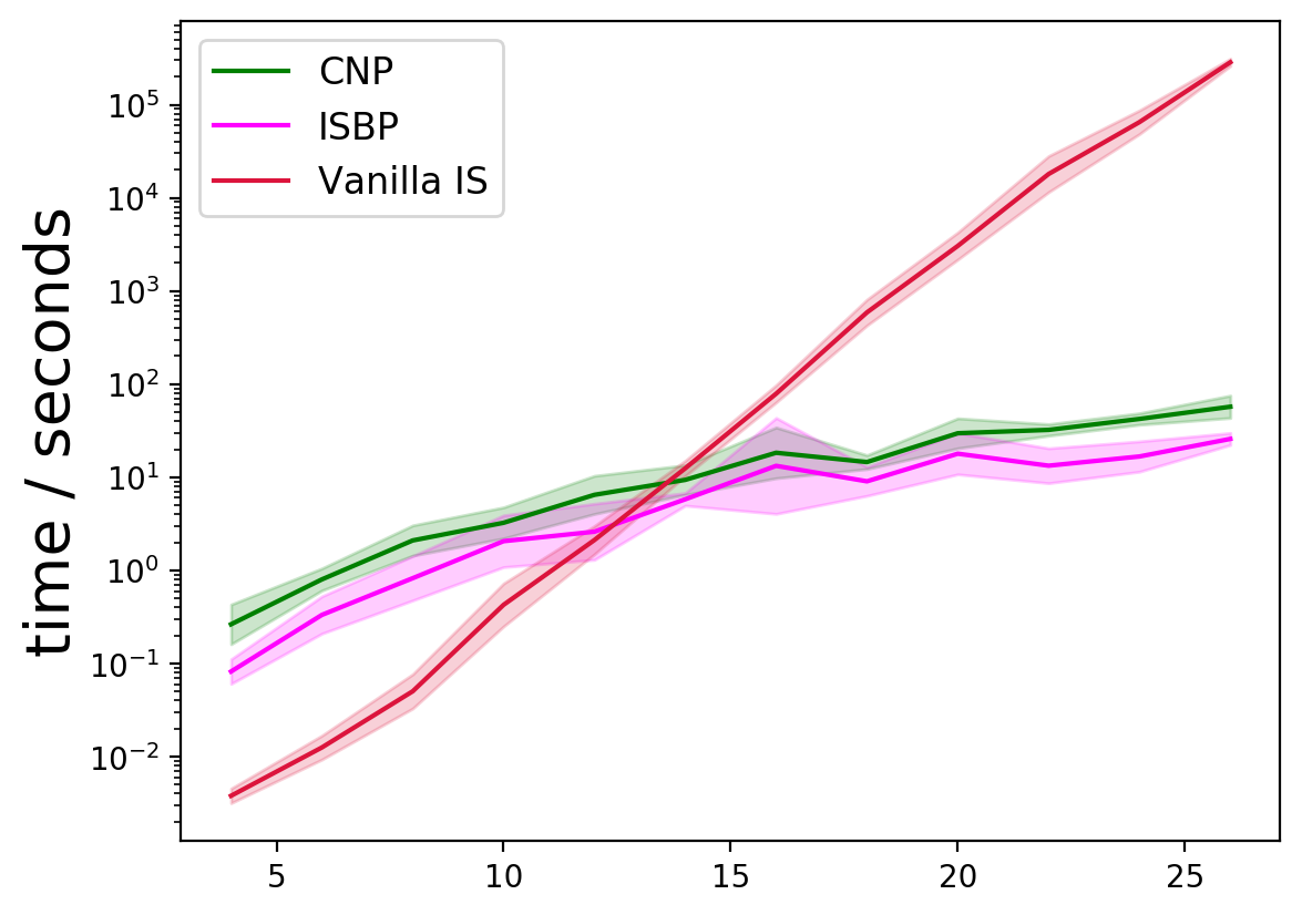
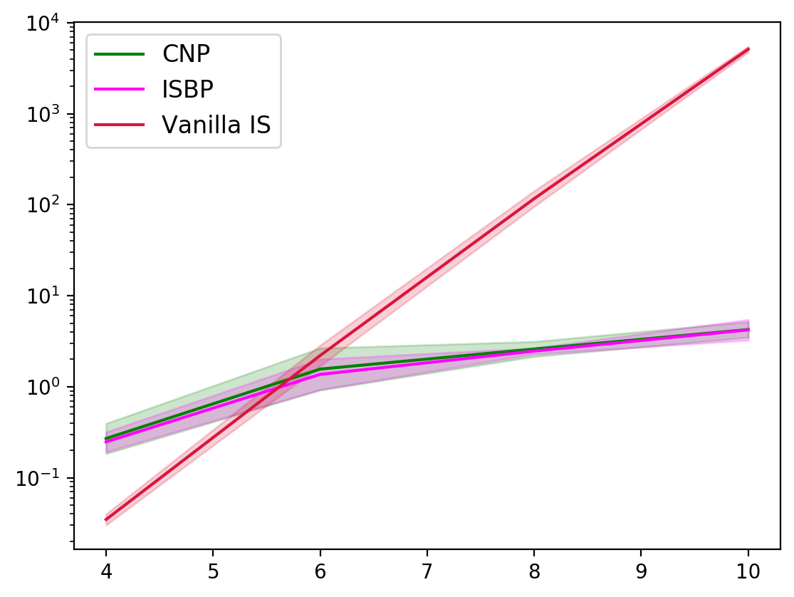
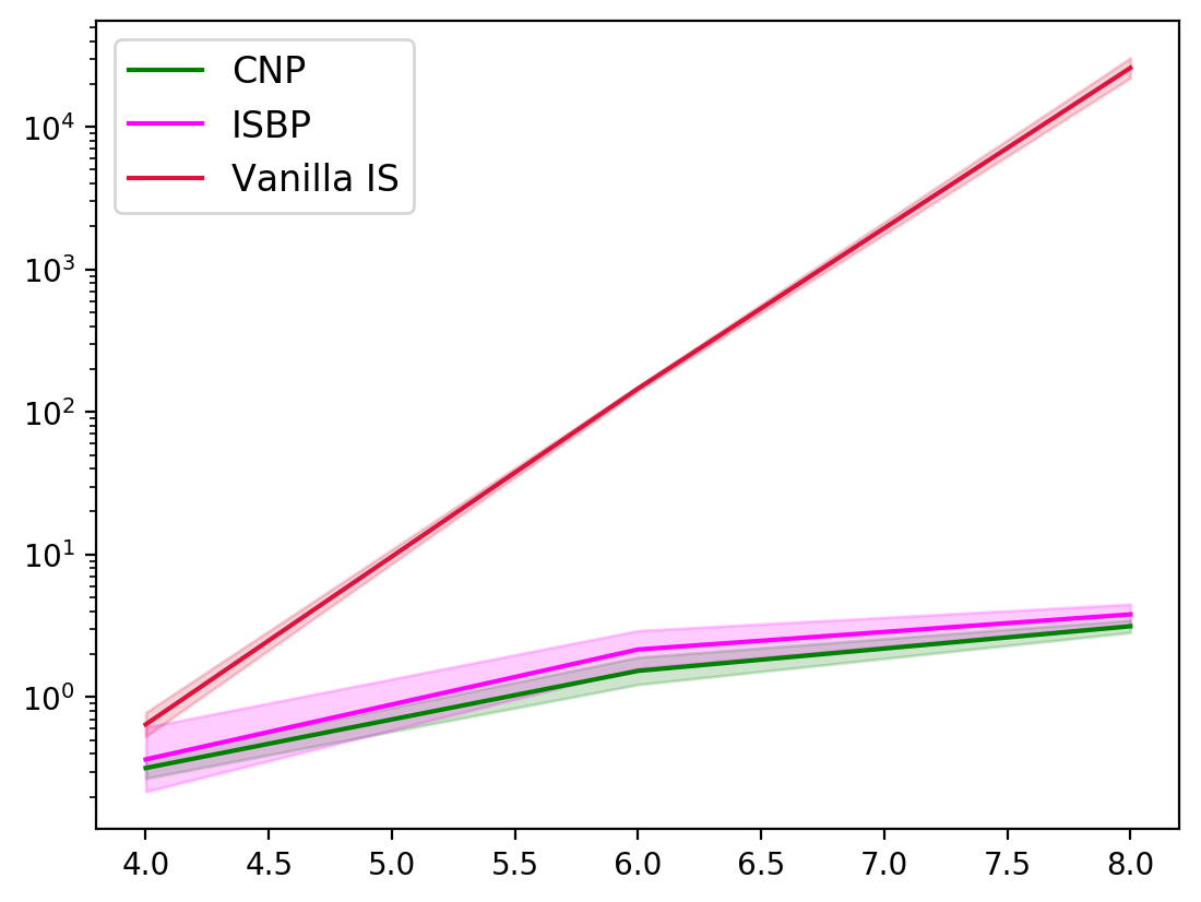
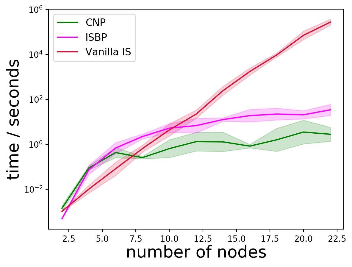
Multi-marginal optimal transport and
probabilistic graphical models

Isabel Haasler, Rahul Singh, Qinsheng Zhang, Johan Karlsson, and Yongxin Chen This work was supported by the Swedish Research Council (VR), grant 2014-5870, SJTU-KTH cooperation grant and the NSF under grant 1901599 and 1942523. I. Haasler and J. Karlsson are with the Division of Optimization and Systems Theory, Department of Mathematics, KTH Royal Institute of Technology, Stockholm, Sweden. haasler@kth.se, johan.karlsson@math.kth.seR. Singh, Q. Zhang and Y. Chen are with the School of Aerospace Engineering, Georgia Institute of Technology, Atlanta, GA, USA. {qzhang419,rasingh,yongchen}@gatech.eduI. Haasler, R. Singh and Q. Zhang contribute equally to this paper.
Abstract

We study multi-marginal optimal transport problems from a probabilistic graphical model perspective. We point out an elegant connection between the two when the underlying cost for optimal transport allows a graph structure. In particular, an entropy regularized multi-marginal optimal transport is equivalent to a Bayesian marginal inference problem for probabilistic graphical models with the additional requirement that some of the marginal distributions are specified. This relation on the one hand extends the optimal transport as well as the probabilistic graphical model theories, and on the other hand leads to fast algorithms for multi-marginal optimal transport by leveraging the well-developed algorithms in Bayesian inference. Several numerical examples are provided to highlight the results.

Index Terms:
Optimal transport, Probabilistic graphical models, Belief Propagation, Norm-product, Iterative Scaling, Bayesian inference.

I Introduction

Optimal transport (OT) theory [1, 2] is a powerful tool in the study of probability distributions. The subject dates back to 1781, when the civil engineer Monge aimed to find an optimal strategy to move soil to road construction sites. Over 200 years of development have brought OT far beyond a civil engineering problem to a compelling mathematical framework which has found applications in economics, signal and image processing, systems and controls, statistics, and machine learning [3, 4, 5, 6, 7, 8, 9]. The inherent properties of OT make it especially suitable for handling high-dimensional data with low-dimensional structure, which is the case in most machine learning settings. Thanks to the discoveries of several efficient algorithms such as iterative scaling, also called Sinkhorn iterations [10], OT has become a powerful framework for a range of machine learning problems. In the 30s this algorithm has also been studied in the statistics community under the name contingence table [11].

The aim of standard OT problems is to find a joint distribution of two given marginals that minimizes the total transportation cost between them. In some applications, such as incompressible fluid flow modeling, video prediction, tomography, and information fusion problems, more than two marginal distributions are given. To tackle these problems, a multi-marginal generalization of OT has been developed, known as multi-marginal optimal transport (MOT) [12, 13, 14, 15, 16]. MOT was first proposed in [14] as a theoretical extension to OT. Since then, the problem has been studied from a theoretical viewpoint [15] as well as computational perspective [16]. It has found applications in signal processing [17], fluid dynamics [18], density functional theory [19, 20], and estimation and control [21, 22]. Many results for the standard OT problem have been extended to the multi-marginal setting. In particular, the iterative scaling method [10] has been generalized to MOT [23]. However, for the multi-marginal setting the computational complexity remains high, especially when the number of marginal distributions is large [16, 24].

On a seemingly different topic, probabilistic graphical models (PGMs) [25, 26, 27] provide a framework for multi-dimensional random variables. They have been used for a large variety of applications including speech recognition, computer vision, communications, and bioinformatics [28, 29, 25, 26]. PGMs capture the dependencies of a set of random variables compactly as a graph, and are an efficient and robust tool to study the relationship of several probabilistic quantities. Moreover, prior knowledge can be easily incorporated in the model. During the last decades, many efficient algorithms have been developed for inference and learning of PGMs. These algorithms leverage the underlying graph structure, making it possible to solve many otherwise extremely difficult problems. Well-known algorithms for the inference problem include, e.g., belief propagation, and the junction tree algorithm [30, 31, 32, 33, 34].

The purpose of this paper is to point out a surprising connection between MOT and PGMs. More precisely, the main contribution of this work is to establish an equivalence between regularized MOT problems, where the cost function is structured according to a graph, and the inference problem for a PGM on the same graph, where some marginal distributions are fixed. This connection leads to a novel interpretation for both MOT and PGMs. On the one hand, MOT can be viewed as an inference problem of a PGM with constraints on some of the marginals, that is, constrained inference problems, and on the other hand, the inference problem of a PGM is a MOT problem, where the available marginals are Dirac distributions.

From a numerical point of view, this connection allows for adapting existing PGM algorithms to this class of MOT problems with graphical structured cost. In this work, we focus on belief propagation (BP) [35, 30] and an extension of it known as norm-product algorithm [36]. These belong to the so called message passing algorithms which exploit the underlying graphical structure, and rely on exchanging information between the nodes. Thus, only local updates are needed, which greatly reduces the computational complexity of the inference problem. If the graphical model is a tree, these algorithms converge globally to the exact conditional marginal distributions in a finite number of iterations. For general PGMs with cycles, there is no convergence guarantee, but both methods usually work well in practice and provide relatively accurate approximations of the marginals. In this work, we develop algorithms for solving entropy regularized MOT problems, or equivalently constrained inference problems, by combining these message passing algorithms with the iterative scaling method. Moreover, we build on earlier results and establish global convergence of our algorithms for tree graphs. Similar constrained inference problems have previously been studied in [37]. Interestingly, the algorithm presented therein is comparable to our proposed extension of the BP algorithm. With the connections to MOT, we provide a new motivation for studying this problem, which also leads to a more complete picture of the algorithms.

A promising application of our framework are in the inference problems for collective dynamics, for instance, in the estimation of the behavior of large groups from only aggregate measurements. Such types of filtering methods are crucial for collective dynamics since it is usually impossible to track the trajectories of each single agent in a large population, due to exploding computational complexity, lack of sensor data or for privacy considerations. Related problems have been studied under the name collective graphical models (CGMs) [38, 39, 40]. These works consider a large collection of identical graphical models, which are observed simultaneously, and aim to infer aggregate distribution over the nodes. Several heuristic algorithms [40] have been proposed to solve the resulting inference problems. Our MOT framework suggest a different observation model [41, 42], which is reasonable in many scenarios. More importantly, our algorithms, which enjoy global convergence guarantee, provide a reliable machine to estimate collective dynamics in these models.

The rest of this paper is structured as follows. In Section II we review some background knowledge in optimal transport and probabilistic graphical models. In Section III we provide the main theoretical result in this paper, which is the equivalence between entropy regularized MOT and the inference problem for PGMs. We also modify the belief propagation algorithm to solve MOT problems. Another algorithm based on the norm-product algorithm is introduced in Section IV. We test and verify our results through several numerical examples in Section V. This is followed by a brief concluding remark in Section VI.

Notation: The notation used throughout is mostly standard. However, with exp()\exp(\cdot), ln()\ln(\cdot), direct-product\odot, and ././ we denote the element-wise exponential, logarithm, multiplication, and division of vectors, matrices, and tensors, respectively. Moreover, tensor-product\otimes denotes the outer product. By 𝟏1{\bf 1} we denote a vector of ones, the size of which will be clear from the context. Throughout, we use bold symbols to represent vectors, e.g., 𝐛j,𝝁jsubscript𝐛𝑗subscript𝝁𝑗{\mathbf{b}}_{j},\boldsymbol{\mu}_{j}, and regular symbol for the corresponding entries, e.g., bj(xj),μj(xj)subscript𝑏𝑗subscript𝑥𝑗subscript𝜇𝑗subscript𝑥𝑗b_{j}(x_{j}),\mu_{j}(x_{j}).

II Preliminaries

In this section, we provide a quick overview of optimal transport theory, probabilistic graphical models and belief propagation algorithm. We only cover material that is most relevant to this work. The reader is referred to [2, 25, 26] for more details.

II-A Optimal transport

In optimal transport (OT) problems, one seeks an optimal plan that transports mass from a source distribution to a target distribution with minimum cost. In its original formulation [43], OT was studied over Euclidean space. However, in general, OT problems can be formulated in both continuous space and discrete space. In this work, we focus on optimal transport over discrete space.

Let 𝝁1+d1,𝝁2+d2formulae-sequencesubscript𝝁1superscriptsubscriptsubscript𝑑1subscript𝝁2superscriptsubscriptsubscript𝑑2\boldsymbol{\mu}_{1}\in{\mathbb{R}}_{+}^{d_{1}},\boldsymbol{\mu}_{2}\in{\mathbb{R}}_{+}^{d_{2}} be two discrete distributions, viz., nonnegative vectors, with equal mass, that is i1μ1(i1)=i2μ2(i2)subscriptsubscript𝑖1subscript𝜇1subscript𝑖1subscriptsubscript𝑖2subscript𝜇2subscript𝑖2\sum_{i_{1}}\mu_{1}(i_{1})=\sum_{i_{2}}\mu_{2}(i_{2}). Here μ1(i)subscript𝜇1𝑖\mu_{1}(i) denotes the amount of mass in the source distribution at location i𝑖i and μ2(i)subscript𝜇2𝑖\mu_{2}(i) denotes the amount of mass in the target distribution at location i𝑖i. Without loss of generality, we assume that both 𝝁1subscript𝝁1\boldsymbol{\mu}_{1} and 𝝁2subscript𝝁2\boldsymbol{\mu}_{2} are probability vectors, that is, the total mass is i1μ1(i1)=i2μ2(i2)=1subscriptsubscript𝑖1subscript𝜇1subscript𝑖1subscriptsubscript𝑖2subscript𝜇2subscript𝑖21\sum_{i_{1}}\mu_{1}(i_{1})=\sum_{i_{2}}\mu_{2}(i_{2})=1. The transport cost of moving a unit mass from point i1subscript𝑖1i_{1} to i2subscript𝑖2i_{2} is denoted by C(i1,i2)𝐶subscript𝑖1subscript𝑖2C(i_{1},i_{2}), and collected in the matrix 𝐂=[C(i1,i2)]d1×d2𝐂delimited-[]𝐶subscript𝑖1subscript𝑖2superscriptsubscript𝑑1subscript𝑑2{\bf C}=[C(i_{1},i_{2})]\in{\mathbb{R}}^{d_{1}\times d_{2}}. In the Kantorovich formulation [44] of OT, the goal is to find a transport plan between the two marginal distributions 𝝁1subscript𝝁1\boldsymbol{\mu}_{1} and 𝝁2subscript𝝁2\boldsymbol{\mu}_{2} that minimizes the total transport cost. A transport plan is encoded in a joint probability matrix 𝐁=[B(i1,i2)]+d1×d2𝐁delimited-[]𝐵subscript𝑖1subscript𝑖2superscriptsubscriptsubscript𝑑1subscript𝑑2{\mathbf{B}}=[B(i_{1},i_{2})]\in{\mathbb{R}}_{+}^{d_{1}\times d_{2}} of 𝝁1,𝝁2subscript𝝁1subscript𝝁2\boldsymbol{\mu}_{1},\boldsymbol{\mu}_{2}. Then the total transport cost is i1,i2C(i1,i2)B(i1,i2)=trace(𝐂T𝐁)subscriptsubscript𝑖1subscript𝑖2𝐶subscript𝑖1subscript𝑖2𝐵subscript𝑖1subscript𝑖2tracesuperscript𝐂𝑇𝐁\sum_{i_{1},i_{2}}C(i_{1},i_{2})B(i_{1},i_{2})=\operatorname{trace}({\bf C}^{T}{\mathbf{B}}) and therefore the OT problem reads

min𝐁+d1×d2subscript𝐁superscriptsubscriptsubscript𝑑1subscript𝑑2\displaystyle\min_{{\mathbf{B}}\in{\mathbb{R}}_{+}^{d_{1}\times d_{2}}}{} trace(𝐂T𝐁)tracesuperscript𝐂𝑇𝐁\displaystyle\operatorname{trace}({\bf C}^{T}{\mathbf{B}}) (1)
subject to 𝐁𝟏=𝝁1𝐁𝟏subscript𝝁1\displaystyle{\mathbf{B}}{\bf 1}=\boldsymbol{\mu}_{1}
𝐁T𝟏=𝝁2,superscript𝐁𝑇1subscript𝝁2\displaystyle{\mathbf{B}}^{T}{\bf 1}=\boldsymbol{\mu}_{2},

where 𝟏1{\bf 1} denotes a vector of ones of proper dimension. The constraints are to enforce that 𝐁𝐁{\mathbf{B}} is a joint distribution between 𝝁1subscript𝝁1\boldsymbol{\mu}_{1} and 𝝁2subscript𝝁2\boldsymbol{\mu}_{2}.

Even though the above OT problem (1) is a linear program, in many practical applications it is too difficult to be solved directly using standard solvers due to the large number of variables [23, 17], especially in the case where the marginal distributions 𝝁1,𝝁2subscript𝝁1subscript𝝁2\boldsymbol{\mu}_{1},\boldsymbol{\mu}_{2} come from discretizations of continuous measures. Recently, a regularization of OT [10] was proposed that greatly reduces the computational complexity of (approximately) solving OT problems over discrete space. In this method, an entropy term

(𝐁)=i1,i2B(i1,i2)lnB(i1,i2)𝐁subscriptsubscript𝑖1subscript𝑖2𝐵subscript𝑖1subscript𝑖2𝐵subscript𝑖1subscript𝑖2{\mathcal{H}}({\mathbf{B}})=-\sum_{i_{1},i_{2}}B(i_{1},i_{2})\ln\,B(i_{1},i_{2}) (2)

is added to regularize the problem, leading to

min𝐁+d1×d2subscript𝐁superscriptsubscriptsubscript𝑑1subscript𝑑2\displaystyle\min_{{\mathbf{B}}\in{\mathbb{R}}_{+}^{d_{1}\times d_{2}}}{} trace(𝐂T𝐁)ϵ(𝐁)tracesuperscript𝐂𝑇𝐁italic-ϵ𝐁\displaystyle\operatorname{trace}({\bf C}^{T}{\mathbf{B}})-\epsilon{\mathcal{H}}({\mathbf{B}}) (3)
subject to 𝐁𝟏=𝝁1𝐁𝟏subscript𝝁1\displaystyle{\mathbf{B}}{\bf 1}=\boldsymbol{\mu}_{1}
𝐁T𝟏=𝝁2,superscript𝐁𝑇1subscript𝝁2\displaystyle{\mathbf{B}}^{T}{\bf 1}=\boldsymbol{\mu}_{2},

where ϵ>0italic-ϵ0\epsilon>0 is a regularization parameter. The entropy regularized OT problem (3) is strictly convex and thus the solution is unique. More importantly, it can be solved efficiently via the Sinkhorn algorithm [45, 10], also known as iterative scaling [11, 46]. Let 𝐊=[K(i1,i2)]d1×d2𝐊delimited-[]𝐾subscript𝑖1subscript𝑖2superscriptsubscript𝑑1subscript𝑑2{\bf K}=[K(i_{1},i_{2})]\in{\mathbb{R}}^{d_{1}\times d_{2}} be defined as K(i1,i2)=exp(C(i1,i2)/ϵ)𝐾subscript𝑖1subscript𝑖2𝐶subscript𝑖1subscript𝑖2italic-ϵK(i_{1},i_{2})=\exp(-C(i_{1},i_{2})/\epsilon), then the iterative scaling updates alternate between the two steps

𝐮1𝝁1./𝐊𝐮2,𝐮2𝝁2./𝐊T𝐮1,{\mathbf{u}}_{1}\leftarrow\boldsymbol{\mu}_{1}./{\bf K}{\mathbf{u}}_{2},\quad{\mathbf{u}}_{2}\leftarrow\boldsymbol{\mu}_{2}./{\bf K}^{T}{\mathbf{u}}_{1}, (4)

where ././ denotes element-wise division. The algorithm converges linearly to a unique pair of vectors 𝐮1d1,𝐮2d2formulae-sequencesubscript𝐮1superscriptsubscript𝑑1subscript𝐮2superscriptsubscript𝑑2{\mathbf{u}}_{1}\in{\mathbb{R}}^{d_{1}},{\mathbf{u}}_{2}\in{\mathbb{R}}^{d_{2}} up to a normalization [46]. Given the limit point of the iteration, the solution to (3) has the form

𝐁=diag(𝐮1)𝐊diag(𝐮2),𝐁diagsubscript𝐮1𝐊diagsubscript𝐮2{\mathbf{B}}=\operatorname{diag}({\mathbf{u}}_{1}){\bf K}\operatorname{diag}({\mathbf{u}}_{2}), (5)

that is, B(i1,i2)=K(i1,i2)u1(i1)u2(i2)𝐵subscript𝑖1subscript𝑖2𝐾subscript𝑖1subscript𝑖2subscript𝑢1subscript𝑖1subscript𝑢2subscript𝑖2B(i_{1},i_{2})=K(i_{1},i_{2})u_{1}(i_{1})u_{2}(i_{2}) for all 1i1d1,1i2d2formulae-sequence1subscript𝑖1subscript𝑑11subscript𝑖2subscript𝑑21\leq i_{1}\leq d_{1},1\leq i_{2}\leq d_{2}.

II-B Probabilistic graphical models

A probabilistic graphical model (PGM) is a graph-based representation of a collection of random vectors that captures the conditional dependencies between them. It provides a compact representation of their joint distributions through factorization: a graphical model consists of a collection of distributions that factorize according to an underlying graph structure. In this work we focus on undirected graphs, which represent Markov random fields [25]. Note that directed graphs represent Bayesian networks, and can always be transformed into a Markov random field [26].

Among the many representations for Markov random fields, the factor graph representation has been widely used due to its elegance and flexibility [25], and is also used in this paper. Consider a graphical model with underlying factor graph G=(V,F,E)𝐺𝑉𝐹𝐸G=(V,\,F,\,E) where V𝑉V denotes the set of variable nodes, F𝐹F denotes the set and factor nodes, and E𝐸E stands for the edges connecting them (see Figure 1 for an example). In such a factor graph G𝐺G, the neighbors of a node jV𝑗𝑉j\in V consists of factor nodes, N(j)F𝑁𝑗𝐹N(j)\subset F, and the neighbors of a factor node αF𝛼𝐹\alpha\in F are variable nodes N(α)V𝑁𝛼𝑉N(\alpha)\subset V. Therefore, G𝐺G is a bipartite graph [47]. Each variable node jV𝑗𝑉j\in V is associated with a random variable xjsubscript𝑥𝑗x_{j} which can be either discrete or continuous. Here we consider only the discrete cases and assume that the random variable xjsubscript𝑥𝑗x_{j} can take djsubscript𝑑𝑗d_{j} possible values. Each factor node αF𝛼𝐹\alpha\in F corresponds to the dependence between the variable nodes connected to α𝛼\alpha, which are compactly denoted by 𝐱α:={xj;jN(α)}assignsubscript𝐱𝛼subscript𝑥𝑗𝑗𝑁𝛼{\bf x}_{\alpha}:=\{x_{j}~{};~{}j\in N(\alpha)\}. In Markov random fields with underlying factor graph G𝐺G, the joint probability is assumed to be of the form

p(𝐱):=p(x1,x2,,xJ)=1ZjVϕj(xj)αFψα(𝐱α)assign𝑝𝐱𝑝subscript𝑥1subscript𝑥2subscript𝑥𝐽1𝑍subscriptproduct𝑗𝑉subscriptitalic-ϕ𝑗subscript𝑥𝑗subscriptproduct𝛼𝐹subscript𝜓𝛼subscript𝐱𝛼p({\bf x}):=p(x_{1},x_{2},\ldots,x_{J})=\frac{1}{Z}\prod_{j\in V}\phi_{j}(x_{j})\prod_{\alpha\in F}\psi_{\alpha}({\mathbf{x}}_{\alpha}) (6)

where ϕjsubscriptbold-italic-ϕ𝑗\boldsymbol{\phi}_{j} is the node/local potential corresponding to node j𝑗j, 𝝍αsubscript𝝍𝛼\boldsymbol{\psi}_{\alpha} is the factor node potential corresponding to factor node α𝛼\alpha, and Z𝑍Z is a normalization constant. A factor node potential ψαsubscript𝜓𝛼\psi_{\alpha} describes the dependence between random variables in {xj;jN(α)}subscript𝑥𝑗𝑗𝑁𝛼\{x_{j}~{};~{}j\in N(\alpha)\}. The node potentials normally come from two sources: prior belief and evidence from measurements. In the latter, ϕj(xj)subscriptitalic-ϕ𝑗subscript𝑥𝑗\phi_{j}(x_{j}) is short for ϕj(xj,yj)subscriptitalic-ϕ𝑗subscript𝑥𝑗subscript𝑦𝑗\phi_{j}(x_{j},y_{j}) [33] with yjsubscript𝑦𝑗y_{j} being the measurement. In cases where all the local potentials are induced by evidence, a more precise formula for the model is

p(𝐱)=1ZjVϕj(xj,yj)αFψα(𝐱α).𝑝𝐱1𝑍subscriptproduct𝑗𝑉subscriptitalic-ϕ𝑗subscript𝑥𝑗subscript𝑦𝑗subscriptproduct𝛼𝐹subscript𝜓𝛼subscript𝐱𝛼p({\bf x})=\frac{1}{Z}\prod_{j\in V}\phi_{j}(x_{j},y_{j})\prod_{\alpha\in F}\psi_{\alpha}({\mathbf{x}}_{\alpha}). (7)

Since the measurement is usually specified in inference problems, yjsubscript𝑦𝑗y_{j} is often neglected to simplify the notation. In principle, the node potentials can be fully absorbed into the factor potentials, that is, the joint distribution becomes p(𝐱)αFψα(𝐱α)proportional-to𝑝𝐱subscriptproduct𝛼𝐹subscript𝜓𝛼subscript𝐱𝛼p({\bf x})\propto\prod_{\alpha\in F}\psi_{\alpha}({\mathbf{x}}_{\alpha}). For the ease of presentation, we adopt the formulation (6).

Apart from factor graphs, another popular representation of PGMs is the standard graph where the nodes are all variables. In the standard graph representation, the dependence between the variables are fully captured by the edges of the graphs. The two representations are equivalent and one can transform one to another easily as the following example illustrates.

Example 1.

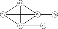
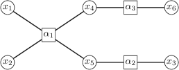
The factor graph in Figure 1(a) models the joint distribution

p(x1,,x6)=1Zψα1(𝐱α1)ψα2(𝐱α2)ψα3(𝐱α3)j=16ϕj(xj)𝑝subscript𝑥1subscript𝑥61𝑍subscript𝜓subscript𝛼1subscript𝐱subscript𝛼1subscript𝜓subscript𝛼2subscript𝐱subscript𝛼2subscript𝜓subscript𝛼3subscript𝐱subscript𝛼3superscriptsubscriptproduct𝑗16subscriptitalic-ϕ𝑗subscript𝑥𝑗p(x_{1},\ldots,x_{6})=\frac{1}{Z}\psi_{\alpha_{1}}({\bf x}_{\alpha_{1}})\psi_{\alpha_{2}}({\bf x}_{\alpha_{2}})\psi_{\alpha_{3}}({\bf x}_{\alpha_{3}})\prod_{j=1}^{6}\phi_{j}(x_{j})

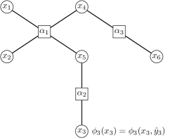
with 𝐱α1={x1,x2,x4,x5}subscript𝐱subscript𝛼1subscript𝑥1subscript𝑥2subscript𝑥4subscript𝑥5{\bf x}_{\alpha_{1}}=\{x_{1},x_{2},x_{4},x_{5}\}, 𝐱α2={x3,x5}subscript𝐱subscript𝛼2subscript𝑥3subscript𝑥5{\bf x}_{\alpha_{2}}=\{x_{3},x_{5}\}, 𝐱α3={x4,x6}subscript𝐱subscript𝛼3subscript𝑥4subscript𝑥6{\bf x}_{\alpha_{3}}=\{x_{4},x_{6}\}. To convert this into a standard graph representation, the dependence among variables induced by the three factors have to be translated to edges. This is straightforward for factors 𝛙α2subscript𝛙subscript𝛼2\boldsymbol{\psi}_{\alpha_{2}} and 𝛙α3subscript𝛙subscript𝛼3\boldsymbol{\psi}_{\alpha_{3}}. The factor 𝛙α1subscript𝛙subscript𝛼1\boldsymbol{\psi}_{\alpha_{1}} involves 444 variables and is more complicated. Without further assumptions on the structure of this factor, it may induce dependence among all of the 444 variables, and thus a complete graph connecting them is required (see Figure 1(b)).
Refer to caption
(a)
Refer to caption
(b)
Figure 1: Factor graph representation vs standard graph representation.

The two fundamental problems in PGMs are inference and learning. Learning refers to estimating the underlying graphical models (often the parametrized factors) using available data sampled from the models. In inference problems, the parameters of the models are given. Instead, the goal is to infer the statistics of the node variables. The two main approaches to inference problems are maximum a posteriori estimation and Bayesian marginal inference [25]. Given a set of measurements {y1,y2,,yJ}subscript𝑦1subscript𝑦2subscript𝑦𝐽\{y_{1},y_{2},\ldots,y_{J}\}, the aim of maximum a posteriori estimation is to find the most likely variable value {x1,x2,,xJ}subscript𝑥1subscript𝑥2subscript𝑥𝐽\{x_{1},x_{2},\ldots,x_{J}\} given the model and measurements. Instead, Bayesian inference calculates the posterior marginal distributions of each node. The focus of this paper is most relevant to Bayesian/marginal inference.

Formally, given a graphical model (6), the objective of Bayesian inference is to calculate marginal distributions p(xj)𝑝subscript𝑥𝑗p(x_{j}) for jV𝑗𝑉j\in V. In cases where the nodes variables are discrete, the marginal p(xj)𝑝subscript𝑥𝑗p(x_{j}) is defined to be

p(xj)=x1,,xj1,xj+1,,xJp(𝐱)=1Zx1,,xj1,xj+1,,xJiVϕi(xi)αFψα(𝐱α).𝑝subscript𝑥𝑗subscriptsubscript𝑥1subscript𝑥𝑗1subscript𝑥𝑗1subscript𝑥𝐽𝑝𝐱1𝑍subscriptsubscript𝑥1subscript𝑥𝑗1subscript𝑥𝑗1subscript𝑥𝐽subscriptproduct𝑖𝑉subscriptitalic-ϕ𝑖subscript𝑥𝑖subscriptproduct𝛼𝐹subscript𝜓𝛼subscript𝐱𝛼p(x_{j})=\sum_{x_{1},\ldots,x_{j-1},x_{j+1},\ldots,x_{J}}p({\bf x})=\frac{1}{Z}\sum_{x_{1},\ldots,x_{j-1},x_{j+1},\ldots,x_{J}}\prod_{i\in V}\phi_{i}(x_{i})\prod_{\alpha\in F}\psi_{\alpha}(\mathbf{x}_{\alpha}). (8)

The Bayesian inference problem can be reformulated as the optimization problem of minimizing

min𝐛(𝐛):=𝒰(𝐛)(𝐛),assignsubscript𝐛𝐛𝒰𝐛𝐛\min_{\mathbf{b}}{\mathcal{F}}({\mathbf{b}}):={\mathcal{U}}({\mathbf{b}})-{\mathcal{H}}({\mathbf{b}}), (9)

with

𝒰(𝐛)=𝐱b(𝐱)(jVlnϕj(xj)+αFlnψα(𝐱α))𝒰𝐛subscript𝐱𝑏𝐱subscript𝑗𝑉subscriptitalic-ϕ𝑗subscript𝑥𝑗subscript𝛼𝐹subscript𝜓𝛼subscript𝐱𝛼{\mathcal{U}}({\mathbf{b}})=-\sum_{\bf x}b({\bf x})\left(\sum_{j\in V}\ln\phi_{j}(x_{j})+\sum_{\alpha\in F}\ln\psi_{\alpha}(\mathbf{x}_{\alpha})\right) (10)

and

(𝐛)=b(𝐱)lnb(𝐱)𝐛𝑏𝐱𝑏𝐱{\mathcal{H}}({\mathbf{b}})=-\sum b({\bf x})~{}\ln~{}b({\bf x}) (11)

over the space of all the probability distributions on 𝐱𝐱{\bf x}. By convention, ,𝒰,𝒰{\mathcal{F}},{\mathcal{U}},{\mathcal{H}} are known as free energy, average energy and entropy respectively due to their similarity to thermodynamics [48]. To see this, we note that the Kullback-Leibler (KL) divergence [49] between b(𝐱)𝑏𝐱b({\bf x}) and p(𝐱)𝑝𝐱p({\bf x}) is

KL(𝐛𝐩):=𝐱b(𝐱)lnb(𝐱)p(𝐱)=𝐱b(𝐱)lnb(𝐱)1/ZjVϕj(xj)αFψα(𝐱α)=F(𝐛)+lnZ.assignKLconditional𝐛𝐩subscript𝐱𝑏𝐱𝑏𝐱𝑝𝐱subscript𝐱𝑏𝐱𝑏𝐱1𝑍subscriptproduct𝑗𝑉subscriptitalic-ϕ𝑗subscript𝑥𝑗subscriptproduct𝛼𝐹subscript𝜓𝛼subscript𝐱𝛼𝐹𝐛𝑍{\rm KL}({\mathbf{b}}\mid{\mathbf{p}}):=\sum_{\bf x}b({\bf x})\ln\frac{b({\bf x})}{p({\bf x})}=\sum_{\bf x}b({\bf x})\ln\frac{b({\bf x})}{1/Z\prod_{j\in V}\phi_{j}(x_{j})\prod_{\alpha\in F}\psi_{\alpha}(\mathbf{x}_{\alpha})}=F({\mathbf{b}})+\ln Z.

Since the KL divergence is nonnegative and equals 00 only if 𝐛=𝐩𝐛𝐩{\mathbf{b}}={\mathbf{p}}, the unique minimizer of (𝐛)𝐛{\mathcal{F}}({\mathbf{b}}) is 𝐩𝐩{\mathbf{p}} with the associated minimum being lnZ𝑍-\ln Z. The optimization formulation (9) of Bayesian inference is the basis for variational inference [25], one of the most popular approximate inference techniques. In the variational inference approach, the approximate distribution 𝐛𝐛{\mathbf{b}} is usually assumed to have some simple structure to ease the optimization, e.g., the mean field approximation b(𝐱)=b1(x1)bJ(xJ)𝑏𝐱subscript𝑏1subscript𝑥1subscript𝑏𝐽subscript𝑥𝐽b({\bf x})=b_{1}(x_{1})\cdots b_{J}(x_{J}) [50]. This work is not concerned with variational inference; (9) simply serves as a link to connect Bayesian inference with optimization. In the PGM literature [51, 36], it is common to introduce a temperature coefficient ϵ>0italic-ϵ0\epsilon>0 into (9), which leads to a slightly more general optimization problem

min𝐛(𝐛)=𝒰(𝐛)ϵ(𝐛).subscript𝐛𝐛𝒰𝐛italic-ϵ𝐛\min_{\mathbf{b}}~{}{\mathcal{F}}({\mathbf{b}})={\mathcal{U}}({\mathbf{b}})-\epsilon{\mathcal{H}}({\mathbf{b}}). (12)

It corresponds to the Bayesian inference for the model

pϵ(𝐱)=1ZjVϕj(xj)ϵαFψα(𝐱α)ϵ.subscript𝑝italic-ϵ𝐱1𝑍subscriptproduct𝑗𝑉subscriptitalic-ϕ𝑗superscriptsubscript𝑥𝑗italic-ϵsubscriptproduct𝛼𝐹subscript𝜓𝛼superscriptsubscript𝐱𝛼italic-ϵp_{\epsilon}({\bf x})=\frac{1}{Z}\prod_{j\in V}\phi_{j}(x_{j})^{\epsilon}\prod_{\alpha\in F}\psi_{\alpha}(\mathbf{x}_{\alpha})^{\epsilon}.

From an optimization point of view, (12) is a regularized version of the linear program

min𝐛𝒰(𝐛).subscript𝐛𝒰𝐛\min_{\mathbf{b}}~{}{\mathcal{U}}({\mathbf{b}}).

Interestingly, this linear program in fact corresponds to the maximum a posteriori problem [36] for the model (6).

II-C Belief Propagation

In principle, Bayesian inference is achievable through the definition (8) by calculating the marginals using brute force summation. The complexity of this summation however scales exponentially as the number of variable nodes J𝐽J goes up [33]. Also the normalization factor Z𝑍Z is extremely difficult to calculate when J𝐽J is large due to the same reason.

During the last two decades, many methods have been developed to solve or approximately solve Bayesian marginal inference problems. One of the most widely used methods is a message-passing algorithm called Belief Propagation [35]. It updates the marginal distribution of each node through communications of beliefs/messages between them. In the factor graph representation, it reads

mαj(xj)subscript𝑚𝛼𝑗subscript𝑥𝑗\displaystyle m_{\alpha\rightarrow j}(x_{j}) proportional-to\displaystyle\propto 𝐱α\xjψα(𝐱α)iN(α)\jniα(xi)subscript\subscript𝐱𝛼subscript𝑥𝑗subscript𝜓𝛼subscript𝐱𝛼subscriptproduct𝑖\𝑁𝛼𝑗subscript𝑛𝑖𝛼subscript𝑥𝑖\displaystyle\sum_{{\bf x}_{\alpha}\backslash x_{j}}\psi_{\alpha}({\bf x}_{\alpha})\prod_{i\in N(\alpha)\backslash j}n_{i\rightarrow\alpha}(x_{i}) (13a)
njα(xj)subscript𝑛𝑗𝛼subscript𝑥𝑗\displaystyle n_{j\rightarrow\alpha}(x_{j}) proportional-to\displaystyle\propto ϕj(xj)βN(j)\αmβj(xj),subscriptitalic-ϕ𝑗subscript𝑥𝑗subscriptproduct𝛽\𝑁𝑗𝛼subscript𝑚𝛽𝑗subscript𝑥𝑗\displaystyle\phi_{j}(x_{j})\prod_{\beta\in N(j)\backslash\alpha}m_{\beta\rightarrow j}(x_{j}), (13b)

where mαj(xj)subscript𝑚𝛼𝑗subscript𝑥𝑗m_{\alpha\rightarrow j}(x_{j}) denotes the message from factor node α𝛼\alpha to variable node j𝑗j, and njα(xj)subscript𝑛𝑗𝛼subscript𝑥𝑗n_{j\rightarrow\alpha}(x_{j}) represents the message from variable node j𝑗j to factor node α𝛼\alpha. The symbol proportional-to\propto means “proportional to” and indicates that often a normalization is applied in the Belief Propagation algorithm. The messages in (13) are updated iteratively over the factor graph.

The Belief Propagation algorithm was first invented to solve Bayesian inference program over trees, in which case global convergence is guaranteed [35, 33]. This method was later generalized to deal with inference problems involving general graphs under the name Loopy Belief Propagation [30]. Even though there is no convergence proof and the algorithm does diverge in some occasions, it works well in practice and is widely adopted. When the algorithm converges, one can calculate the beliefs on the variables and factors by

bj(xj)subscript𝑏𝑗subscript𝑥𝑗\displaystyle b_{j}(x_{j}) proportional-to\displaystyle\propto ϕj(xj)αN(j)mαj(xj)subscriptitalic-ϕ𝑗subscript𝑥𝑗subscriptproduct𝛼𝑁𝑗subscript𝑚𝛼𝑗subscript𝑥𝑗\displaystyle\phi_{j}(x_{j})\prod_{\alpha\in N(j)}m_{\alpha\rightarrow j}(x_{j}) (14a)
bα(𝐱α)subscript𝑏𝛼subscript𝐱𝛼\displaystyle b_{\alpha}({\bf x}_{\alpha}) proportional-to\displaystyle\propto ψα(𝐱α)jN(α)njα(xj).subscript𝜓𝛼subscript𝐱𝛼subscriptproduct𝑗𝑁𝛼subscript𝑛𝑗𝛼subscript𝑥𝑗\displaystyle\psi_{\alpha}({\bf x}_{\alpha})\prod_{j\in N(\alpha)}n_{j\rightarrow\alpha}(x_{j}). (14b)

In cases where the factor graph has no cycles (i.e., it is a tree), the beliefs in (14) coincide with the true posterior marginals, that is,

p(xj)𝑝subscript𝑥𝑗\displaystyle p(x_{j}) =\displaystyle= bj(xj),jV,xjformulae-sequencesubscript𝑏𝑗subscript𝑥𝑗for-all𝑗𝑉for-allsubscript𝑥𝑗\displaystyle b_{j}(x_{j}),~{}~{}\forall j\in V,~{}\forall x_{j} (15a)
p(𝐱α)𝑝subscript𝐱𝛼\displaystyle p({\bf x}_{\alpha}) =\displaystyle= bα(𝐱α),αF,𝐱α.formulae-sequencesubscript𝑏𝛼subscript𝐱𝛼for-all𝛼𝐹for-allsubscript𝐱𝛼\displaystyle b_{\alpha}({\bf x}_{\alpha}),~{}~{}\forall\alpha\in F,~{}\forall{\bf x}_{\alpha}. (15b)

For general graphs with cycles, convergence is not guaranteed and even if it does converge, the beliefs in (14) are only approximations of the true marginals p(xj),p(𝐱α)𝑝subscript𝑥𝑗𝑝subscript𝐱𝛼p(x_{j}),\,p({\bf x}_{\alpha}). A remarkable discovery [30, 31] related to (Loopy) Belief Propagation is that if the updates (13) converge, then the beliefs in (14) form a fixed point of the Bethe free energy [30, 31]

Bethe(𝐛)=𝒰Bethe(𝐛)Bethe(𝐛),subscriptBethe𝐛subscript𝒰Bethe𝐛subscriptBethe𝐛{\mathcal{F}}_{\rm Bethe}({\mathbf{b}})={\mathcal{U}}_{\rm Bethe}({\mathbf{b}})-{\mathcal{H}}_{\rm Bethe}({\mathbf{b}}), (16)

where 𝒰Bethe(𝐛)subscript𝒰Bethe𝐛{\mathcal{U}}_{\rm Bethe}({\mathbf{b}}) is the Bethe average energy

𝒰Bethe(𝐛)=αF𝐱αbα(𝐱α)lnψα(𝐱α)jVxjbj(xj)lnϕj(xj)subscript𝒰Bethe𝐛subscript𝛼𝐹subscriptsubscript𝐱𝛼subscript𝑏𝛼subscript𝐱𝛼subscript𝜓𝛼subscript𝐱𝛼subscript𝑗𝑉subscriptsubscript𝑥𝑗subscript𝑏𝑗subscript𝑥𝑗subscriptitalic-ϕ𝑗subscript𝑥𝑗{\mathcal{U}}_{\rm Bethe}({\mathbf{b}})=-\sum_{\alpha\in F}\sum_{{\bf x}_{\alpha}}b_{\alpha}({\bf x}_{\alpha})\ln\psi_{\alpha}({\bf x}_{\alpha})-\sum_{j\in V}\sum_{x_{j}}b_{j}(x_{j})\ln\phi_{j}(x_{j}) (17)

and Bethe(𝐛)subscriptBethe𝐛{\mathcal{H}}_{\rm Bethe}({\mathbf{b}}) is the Bethe entropy

Bethe(𝐛)=αF𝐱αbα(𝐱α)lnbα(𝐱α)+jV(Nj1)xjbj(xj)lnbj(xj)subscriptBethe𝐛subscript𝛼𝐹subscriptsubscript𝐱𝛼subscript𝑏𝛼subscript𝐱𝛼subscript𝑏𝛼subscript𝐱𝛼subscript𝑗𝑉subscript𝑁𝑗1subscriptsubscript𝑥𝑗subscript𝑏𝑗subscript𝑥𝑗subscript𝑏𝑗subscript𝑥𝑗{\mathcal{H}}_{\rm Bethe}({\mathbf{b}})=-\sum_{\alpha\in F}\sum_{{\bf x}_{\alpha}}b_{\alpha}({\bf x}_{\alpha})\ln b_{\alpha}({\bf x}_{\alpha})+\sum_{j\in V}(N_{j}-1)\sum_{x_{j}}b_{j}(x_{j})\ln b_{j}(x_{j}) (18)

with Njsubscript𝑁𝑗N_{j} denoting the degree of the variable node j𝑗j, i.e., Nj=|N(j)|subscript𝑁𝑗𝑁𝑗N_{j}=|N(j)|. In (16), we define 𝐛={𝐛j,𝐛α:jV,αF}𝐛conditional-setsubscript𝐛𝑗subscript𝐛𝛼formulae-sequence𝑗𝑉𝛼𝐹{\mathbf{b}}=\{{\mathbf{b}}_{j},\,{\mathbf{b}}_{\alpha}~{}:~{}j\in V,\,\alpha\in F\}. This is different to 𝐛𝐛{\mathbf{b}} in (9), which is a J𝐽J-mode tensor. For the sake of conciseness, by abuse of notation, we use 𝐛𝐛{\mathbf{b}} in both settings. For a factor tree, the two are connected through the relation b(𝐱)(αFbα(𝐱α))(jVbj(xj)1Nj)similar-to𝑏𝐱subscriptproduct𝛼𝐹subscript𝑏𝛼subscript𝐱𝛼subscriptproduct𝑗𝑉subscript𝑏𝑗superscriptsubscript𝑥𝑗1subscript𝑁𝑗b({\bf x})\sim(\prod_{\alpha\in F}b_{\alpha}({\bf x}_{\alpha}))(\prod_{j\in V}b_{j}(x_{j})^{1-N_{j}}) [25]. In terms of Bethe free energy, the Bayesian inference problem reads

min𝐛subscript𝐛\displaystyle\min_{{\mathbf{b}}} Bethe(𝐛)subscriptBethe𝐛\displaystyle{\mathcal{F}}_{\rm Bethe}({\mathbf{b}}) (19a)
subject to 𝐱α\xjbα(𝐱α)=bj(xj),jV,αN(j),formulae-sequencesubscript\subscript𝐱𝛼subscript𝑥𝑗subscript𝑏𝛼subscript𝐱𝛼subscript𝑏𝑗subscript𝑥𝑗formulae-sequencefor-all𝑗𝑉𝛼𝑁𝑗\displaystyle\sum_{{\bf x}_{\alpha}\backslash x_{j}}b_{\alpha}({\bf x}_{\alpha})=b_{j}(x_{j}),\quad\forall j\in V,\alpha\in N(j), (19c)
𝐱αbα(𝐱α)=1,αF.formulae-sequencesubscriptsubscript𝐱𝛼subscript𝑏𝛼subscript𝐱𝛼1for-all𝛼𝐹\displaystyle\sum_{{\bf x}_{\alpha}}b_{\alpha}({\bf x}_{\alpha})=1,\quad\forall\alpha\in F.

The constraint (19c) is to ensure that 𝐛α,𝐛jsubscript𝐛𝛼subscript𝐛𝑗{\mathbf{b}}_{\alpha},{\mathbf{b}}_{j} are compatible and (19c) is to guarantee that they are in the probability simplex. It is easy to check that when the factor graph has no cycles, the Bethe free energy (16) is strictly convex in the feasible set defined by the constraints (19c)-(19c), and is equal to the free energy (9), i.e., Bethe=subscriptBethe{\mathcal{F}}_{\rm Bethe}={\mathcal{F}}. Thus, (19) is again a convex optimization problem. For general graphs, the Bethe free energy serves as a good approximation of the free energy [31], but is no longer convex.

III Multimarginal optimal transport as Bayesian inference

Multimarginal optimal transport (MOT) extends the OT framework (1) to the setting involving multiple distributions. In particular, in MOT, one aims to find a transport plan among a set of marginals 𝝁1,,𝝁Jsubscript𝝁1subscript𝝁𝐽\boldsymbol{\mu}_{1},\dots,\boldsymbol{\mu}_{J} with J2𝐽2J\geq 2. In this setting, the transport cost is encoded in a tensor 𝐂=[C(i1,i2,,iJ)]d1×d2××dJ𝐂delimited-[]𝐶subscript𝑖1subscript𝑖2subscript𝑖𝐽superscriptsubscript𝑑1subscript𝑑2subscript𝑑𝐽{\bf C}=[C(i_{1},i_{2},\ldots,i_{J})]\in{\mathbb{R}}^{d_{1}\times d_{2}\times\cdots\times d_{J}} where C(i1,i2,,iJ)𝐶subscript𝑖1subscript𝑖2subscript𝑖𝐽C(i_{1},i_{2},\ldots,i_{J}) denotes the unit transporting cost corresponding to the locations i1,i2,,iJsubscript𝑖1subscript𝑖2subscript𝑖𝐽i_{1},i_{2},\ldots,i_{J}, and the transport plan is in the same way described by a J𝐽J-mode tensor 𝐁+d1×d2××dJ𝐁superscriptsubscriptsubscript𝑑1subscript𝑑2subscript𝑑𝐽{\mathbf{B}}\in{\mathbb{R}}_{+}^{d_{1}\times d_{2}\times\cdots\times d_{J}}.

For a given transport plan 𝐁𝐁{\mathbf{B}}, the total cost of transportation is

𝐂,𝐁:=i1,i2,,iJC(i1,i2,,iJ)B(i1,i2,,iJ).assign𝐂𝐁subscriptsubscript𝑖1subscript𝑖2subscript𝑖𝐽𝐶subscript𝑖1subscript𝑖2subscript𝑖𝐽𝐵subscript𝑖1subscript𝑖2subscript𝑖𝐽\langle{\bf C},{\mathbf{B}}\rangle:=\sum_{i_{1},i_{2},\ldots,i_{J}}C(i_{1},i_{2},\ldots,i_{J})B(i_{1},i_{2},\ldots,i_{J}).

Thus, similar to (1), MOT has a linear programming formulation

min𝐁+d1××dJsubscript𝐁superscriptsubscriptsubscript𝑑1subscript𝑑𝐽\displaystyle\min_{{\mathbf{B}}\in{\mathbb{R}}_{+}^{d_{1}\times\dots\times d_{J}}} 𝐂,𝐁𝐂𝐁\displaystyle\langle{\bf C},{\mathbf{B}}\rangle (20)
subject to Pj(𝐁)=𝝁j, for jΓ,formulae-sequencesubscript𝑃𝑗𝐁subscript𝝁𝑗 for 𝑗Γ\displaystyle P_{j}({\mathbf{B}})=\boldsymbol{\mu}_{j},\text{ for }j\in\Gamma,

where Γ{1,2,,J}Γ12𝐽\Gamma\subset\{1,2,\dots,J\} is an index set specifying which marginal distributions are given, and the projection on the j𝑗j-th marginal of 𝐁𝐁{\mathbf{B}} is computed as

Pj(𝐁)=i1,,ij1,ij+1,iJB(i1,,ij1,ij,ij+1,,iJ).subscript𝑃𝑗𝐁subscriptsubscript𝑖1subscript𝑖𝑗1subscript𝑖𝑗1subscript𝑖𝐽𝐵subscript𝑖1subscript𝑖𝑗1subscript𝑖𝑗subscript𝑖𝑗1subscript𝑖𝐽P_{j}({\mathbf{B}})=\sum_{i_{1},\dots,i_{j-1},i_{j+1},i_{J}}B(i_{1},\dots,i_{j-1},i_{j},i_{j+1},\dots,i_{J}). (21)

Note that the standard bi-marginal OT problem (1) is a special case of the MOT problem (20) with J=2𝐽2J=2 and Γ={1,2}Γ12\Gamma=\{1,2\}.

In the original MOT formulation [12, 15], constraints are given on all the marginal distributions, viz., the index set Γ={1,2,,J}Γ12𝐽\Gamma=\{1,2,\dots,J\}. However, in many applications [15, 16, 52], only a subset of marginal distributions are explicitly given. For instance, the Barycenter problem [53] is a MOT where the target distribution is not given. In this work we consider the setting where constraints are only imposed on a subset of marginals, i.e., Γ{1,2,,J}Γ12𝐽\Gamma\subset\{1,2,\dots,J\}.

III-A Entropy regularized MOT

Although MOT (20) is a standard linear program, its complexity grows exponentially as J𝐽J increases. This computational burden can be partly alleviated in an analogous manner as for the classical bi-marginal problem (1), which again yields an iterative scaling algorithm. In particular, similarly to (3), one can add an entropy term

(𝐁)=i1,,iJB(i1,,iJ)lnB(i1,,iJ)𝐁subscriptsubscript𝑖1subscript𝑖𝐽𝐵subscript𝑖1subscript𝑖𝐽𝐵subscript𝑖1subscript𝑖𝐽{\mathcal{H}}({\mathbf{B}})=-\sum_{i_{1},\dots,i_{J}}B(i_{1},\dots,i_{J})\ln~{}B(i_{1},\dots,i_{J}) (22)

to (20) to regularize the problem, resulting in the strictly convex optimization problem

min𝐁d1××dJsubscript𝐁superscriptsubscript𝑑1subscript𝑑𝐽\displaystyle\min_{{\mathbf{B}}\in{\mathbb{R}}^{d_{1}\times\dots\times d_{J}}} 𝐂,𝐁ϵ(𝐁)𝐂𝐁italic-ϵ𝐁\displaystyle\langle{\bf C},{\mathbf{B}}\rangle-\epsilon{\mathcal{H}}({\mathbf{B}}) (23)
subject to Pj(𝐁)=𝝁j, for jΓformulae-sequencesubscript𝑃𝑗𝐁subscript𝝁𝑗 for 𝑗Γ\displaystyle P_{j}({\mathbf{B}})=\boldsymbol{\mu}_{j},\text{ for }j\in\Gamma

with ϵ>0italic-ϵ0\epsilon>0 being a regularization parameter.

For the bi-marginal case, (23) reduces to problem (3). The iterative scaling algorithm (4) can be generalized to the multi-marginal setting [46] in order to solve (23). From an optimization perspective, the iterative scaling algorithm amounts to a coordinate ascent method [54] in the dual problem of (23). The introduction of the entropy term in (23) allows for closed-form expressions for the updates of the dual variables [17]. Utilizing Lagrangian duality theory, one can show that the optimal solution to (23) is of the form

𝐁=𝐊𝐔,𝐁direct-product𝐊𝐔{\mathbf{B}}={\bf K}\odot{\bf U}, (24)

where direct-product\odot denotes element-wise multiplication and the tensors are given by

𝐊=exp(𝐂/ϵ)𝐊𝐂italic-ϵ{\bf K}=\exp(-{\bf C}/\epsilon) (25)

and

𝐔=𝐮1𝐮2𝐮J,𝐔tensor-productsubscript𝐮1subscript𝐮2subscript𝐮𝐽{\bf U}={\mathbf{u}}_{1}\otimes{\mathbf{u}}_{2}\otimes\dots\otimes{\mathbf{u}}_{J}, (26)

where the vectors 𝐮jdjsubscript𝐮𝑗superscriptsubscript𝑑𝑗{\mathbf{u}}_{j}\in\mathbb{R}^{d_{j}} are given by

𝐮j={exp(1J𝝀jϵ), if jΓexp(1J)𝟏, otherwise,subscript𝐮𝑗cases1𝐽subscript𝝀𝑗italic-ϵ if 𝑗Γ1𝐽1 otherwise,{\mathbf{u}}_{j}=\begin{cases}\exp\left(-\frac{1}{J}-\frac{\boldsymbol{\lambda}_{j}}{\epsilon}\right),&\text{ if }j\in\Gamma\\ \exp\left(-\frac{1}{J}\right){\bf 1},&\text{ otherwise,}\end{cases} (27)

and 𝝀jdjsubscript𝝀𝑗superscriptsubscript𝑑𝑗\boldsymbol{\lambda}_{j}\in\mathbb{R}^{d_{j}} is the dual variable corresponding to the constraint Pj(𝐁)=𝝁jsubscript𝑃𝑗𝐁subscript𝝁𝑗P_{j}({\mathbf{B}})=\boldsymbol{\mu}_{j} on the j𝑗j-th marginal. Moreover, the dual of (23) is

max{𝝀j,jΓ}ϵ𝐊,𝐔jΓ𝝀jT𝝁j.subscriptsubscript𝝀𝑗𝑗Γitalic-ϵ𝐊𝐔subscript𝑗Γsuperscriptsubscript𝝀𝑗𝑇subscript𝝁𝑗\max_{\{\boldsymbol{\lambda}_{j},j\in\Gamma\}}-\epsilon\langle{\bf K},{\bf U}\rangle-\sum_{j\in\Gamma}\boldsymbol{\lambda}_{j}^{T}\boldsymbol{\mu}_{j}. (28)

We emphasis that in (28), 𝐔𝐔{\bf U} is a function of the multipliers {𝝀j,jΓ}subscript𝝀𝑗𝑗Γ\{\boldsymbol{\lambda}_{j},j\in\Gamma\} as defined in (26)-(27).

The iterative scaling algorithm iteratively updates the vectors 𝐮jsubscript𝐮𝑗{\mathbf{u}}_{j}, for jΓ𝑗Γj\in\Gamma, in (27) according to

𝐮j𝐮j𝝁j./Pj(𝐊𝐔),{\mathbf{u}}_{j}\leftarrow{\mathbf{u}}_{j}\odot\boldsymbol{\mu}_{j}./P_{j}({\bf K}\odot{\bf U}), (29)

for all jΓ𝑗Γj\in\Gamma. For future reference, we summarize the steps in Algorithm 1.

Algorithm 1 Iterative Scaling Algorithm for MOT
  Compute 𝐊=exp(𝐂/ϵ)𝐊𝐂italic-ϵ{\bf K}=\exp(-{\bf C}/\epsilon)
  Initialize 𝐮1,𝐮2,,𝐮Jsubscript𝐮1subscript𝐮2subscript𝐮𝐽{\mathbf{u}}_{1},{\mathbf{u}}_{2},\ldots,{\mathbf{u}}_{J} to exp(1J)𝟏1𝐽1\exp(-\frac{1}{J})\mathbf{1}
  while not converged do
     for jΓ𝑗Γj\in\Gamma do
        Compute 𝐔=𝐮1𝐮2𝐮J𝐔tensor-productsubscript𝐮1subscript𝐮2subscript𝐮𝐽{\bf U}={\mathbf{u}}_{1}\otimes{\mathbf{u}}_{2}\otimes\dots\otimes{\mathbf{u}}_{J}
        Update 𝐮jsubscript𝐮𝑗{\mathbf{u}}_{j} as 𝐮j𝐮j𝝁j./Pj(𝐊𝐔){\mathbf{u}}_{j}\leftarrow{\mathbf{u}}_{j}\odot\boldsymbol{\mu}_{j}./P_{j}({\bf K}\odot{\bf U})
     end for
  end while

The Iterative Scaling algorithm (Algorithm 1) is a special case of the iterative Bregman projection algorithm [55, 23], which itself is a special case of a dual block coordinate ascent method [56, 57], and thus enjoys a global convergence guarantee [55, 57].

Note that the standard Sinkhorn iterations (4) for the two-marginal case (3) is a special case of Algorithm 1 when J=2𝐽2J=2 and Γ={1,2}Γ12\Gamma=\{1,2\}. Indeed, in this case, Algorithm 1 boils down to iterating

𝐮1𝐮1𝝁1./P1(𝐊𝐔),𝐮2𝐮2𝝁2./P2(𝐊𝐔).{\mathbf{u}}_{1}\leftarrow{\mathbf{u}}_{1}\odot\boldsymbol{\mu}_{1}./P_{1}({\bf K}\odot{\bf U}),\qquad{\mathbf{u}}_{2}\leftarrow{\mathbf{u}}_{2}\odot\boldsymbol{\mu}_{2}./P_{2}({\bf K}\odot{\bf U}).

With P1(𝐊𝐔)=diag(𝐮1)𝐊diag(𝐮2)𝟏=diag(𝐮1)(𝐊𝐮2)=𝐮1(𝐊𝐮2)subscript𝑃1direct-product𝐊𝐔diagsubscript𝐮1𝐊diagsubscript𝐮21diagsubscript𝐮1subscript𝐊𝐮2direct-productsubscript𝐮1subscript𝐊𝐮2P_{1}({\bf K}\odot{\bf U})=\operatorname{diag}({\mathbf{u}}_{1}){\bf K}\operatorname{diag}({\mathbf{u}}_{2}){\bf 1}=\operatorname{diag}({\mathbf{u}}_{1})({\bf K}{\mathbf{u}}_{2})={\mathbf{u}}_{1}\odot({\bf K}{\mathbf{u}}_{2}) and similarly P2(𝐊𝐔)=𝐮2(𝐊T𝐮1)subscript𝑃2direct-product𝐊𝐔direct-productsubscript𝐮2superscript𝐊𝑇subscript𝐮1P_{2}({\bf K}\odot{\bf U})={\mathbf{u}}_{2}\odot({\bf K}^{T}{\mathbf{u}}_{1}), it follows

𝐮1𝝁1./𝐊𝐮2,𝐮2𝝁2./𝐊T𝐮1,{\mathbf{u}}_{1}\leftarrow\boldsymbol{\mu}_{1}./{\bf K}{\mathbf{u}}_{2},\qquad{\mathbf{u}}_{2}\leftarrow\boldsymbol{\mu}_{2}./{\bf K}^{T}{\mathbf{u}}_{1},

which coincide with (4).

Although Algorithm 1 is easy to implement and considerably faster than general linear programming solvers, its complexity still scales exponentially as J𝐽J grows since the number of elements in 𝐁𝐁{\mathbf{B}} are d1d2dJsubscript𝑑1subscript𝑑2subscript𝑑𝐽d_{1}d_{2}\ldots d_{J}. The computational bottleneck of it lies in the calculation of the projections Pj(𝐁)subscript𝑃𝑗𝐁P_{j}({\mathbf{B}}), for jΓ𝑗Γj\in\Gamma, in (21). Generally, this computational burden is inevitable. However, in some cases it is possible to utilize structures in the cost tensor 𝐂𝐂{\bf C} to make the computation of the projections more accessible [23, 17, 52]. In Section III-B we consider MOT problems with cost tensors that can be decomposed according to a graph. This graphical structure allows us to leverage the Bayesian inference tools [26] in PGMs to compute the projections efficiently. Other than providing a workhorse for solving MOT problems with graphical structured cost, this connection between MOT and PGMs also presents new elements and perspective to Bayesian inference in PGMs, which is discussed in details in Section III-C.

III-B MOT with graphical structures

Consider the cases where the cost tensor 𝐂𝐂{\bf C} can be decomposed according to a factor graph. More specifically, the cost tensor 𝐂𝐂{\bf C} has the form

C(𝐱)=αFCα(𝐱α),𝐶𝐱subscript𝛼𝐹subscript𝐶𝛼subscript𝐱𝛼C({\bf x})=\sum_{\alpha\in F}C_{\alpha}({\bf x}_{\alpha}), (30)

where F𝐹F denotes the set of factors of a graph. Here, to be consistent with the notations in PGMs, we write the cost of associating i1,i2,,iJsubscript𝑖1subscript𝑖2subscript𝑖𝐽i_{1},i_{2},\ldots,i_{J} by C(𝐱)=C(x1,x2,,xJ)𝐶𝐱𝐶subscript𝑥1subscript𝑥2subscript𝑥𝐽C({\bf x})=C(x_{1},x_{2},\ldots,x_{J}) instead of C(i1,i2,,iJ)𝐶subscript𝑖1subscript𝑖2subscript𝑖𝐽C(i_{1},i_{2},\ldots,i_{J}), but the two have exactly the same meaning; both xjsubscript𝑥𝑗x_{j} and ijsubscript𝑖𝑗i_{j} take values in a set with djsubscript𝑑𝑗d_{j} elements. Thus, by abuse of notation, we use C(𝐱)𝐶𝐱C({\bf x}) and C(i1,i2,,iJ)𝐶subscript𝑖1subscript𝑖2subscript𝑖𝐽C(i_{1},i_{2},\ldots,i_{J}) interchangeably.

A graph structured cost tensor (30) occurs in various applications of the OT framework [23, 17]. For instance, in Barycenter problems [53], the cost 𝐂𝐂{\bf C} can be decomposed into the sum of pairwise costs between the target distribution and each given marginal distribution. For general cost functions, it might be possible to approximate them using the structured cost (30). Thus the framework we establish can also be viewed as an efficient method to approximate the solution to any MOT problem.

Denote the factor graph associated with the cost (30) by G=(V,F,E)𝐺𝑉𝐹𝐸G=(V,F,E). Then the j𝑗j-th mode of 𝐂𝐂{\bf C} corresponds to node jV𝑗𝑉j\in V and the marginal distribution of the j𝑗j-th mode is the same as the marginal distribution of xjsubscript𝑥𝑗x_{j} at node j𝑗j. In this paper, we only consider the cases where the factor graph G𝐺G is connected but does not have any loop, that is, G𝐺G is a factor tree. We associate the cost 𝐂𝐂{\bf C} with a probabilistic graphical model

p(𝐱)=1ZαFKα(𝐱α)𝑝𝐱1𝑍subscriptproduct𝛼𝐹subscript𝐾𝛼subscript𝐱𝛼p({\bf x})=\frac{1}{Z}\prod_{\alpha\in F}K_{\alpha}({\bf x}_{\alpha})

where

Kα(𝐱α)=exp(Cα(𝐱α)/ϵ).subscript𝐾𝛼subscript𝐱𝛼subscript𝐶𝛼subscript𝐱𝛼italic-ϵK_{\alpha}({\bf x}_{\alpha})=\exp(-C_{\alpha}({\bf x}_{\alpha})/\epsilon). (31)

Clearly, 𝐊𝐊{\bf K} in (25) has the form

𝐊=[K(i1,i2,,iJ)]=[K(𝐱)]=[αFKα(𝐱α)],𝐊delimited-[]𝐾subscript𝑖1subscript𝑖2subscript𝑖𝐽delimited-[]𝐾𝐱delimited-[]subscriptproduct𝛼𝐹subscript𝐾𝛼subscript𝐱𝛼{\bf K}=[K(i_{1},i_{2},\ldots,i_{J})]=[K({\bf x})]=[\prod_{\alpha\in F}K_{\alpha}({\bf x}_{\alpha})],

and

𝐊𝐔=[K(𝐱)U(𝐱)]=[(αFKα(𝐱α))(jVuj(xj))].direct-product𝐊𝐔delimited-[]𝐾𝐱𝑈𝐱delimited-[]subscriptproduct𝛼𝐹subscript𝐾𝛼subscript𝐱𝛼subscriptproduct𝑗𝑉subscript𝑢𝑗subscript𝑥𝑗{\bf K}\odot{\bf U}=[K({\bf x})U({\bf x})]=[\left(\prod_{\alpha\in F}K_{\alpha}({\bf x}_{\alpha})\right)\left(\prod_{j\in V}u_{j}(x_{j})\right)]. (32)

From a PGM point of view, the (transformed) Lagrangian multipliers 𝐮jsubscript𝐮𝑗{\mathbf{u}}_{j}, for jΓ𝑗Γj\in\Gamma, introduced by the Iterative Scaling algorithm are local potentials of the modified graphical model K(𝐱)U(𝐱)𝐾𝐱𝑈𝐱K({\bf x})U({\bf x}). The Lagrangian approach of solving the constrained optimization problem (23) seeks multipliers 𝐮jsubscript𝐮𝑗{\mathbf{u}}_{j}, for jΓ𝑗Γj\in\Gamma, such that the tensor 𝐁=𝐊𝐔𝐁direct-product𝐊𝐔{\mathbf{B}}={\bf K}\odot{\bf U} satisfies all the constraints Pj(𝐁)=𝝁jsubscript𝑃𝑗𝐁subscript𝝁𝑗P_{j}({\mathbf{B}})=\boldsymbol{\mu}_{j}, for jΓ𝑗Γj\in\Gamma. Thus, in the language of PGMs, to solve the MOT problem (23), one can search for a proper set of artificial local potentials 𝐮jsubscript𝐮𝑗{\mathbf{u}}_{j}, for jΓ𝑗Γj\in\Gamma, such that the modified graphical model K(𝐱)U(𝐱)𝐾𝐱𝑈𝐱K({\bf x})U({\bf x}) in (32) has the specified marginal distribution 𝝁jsubscript𝝁𝑗\boldsymbol{\mu}_{j} on the j𝑗j-th variable node for each jΓ𝑗Γj\in\Gamma. Note that 𝐮j=exp(1/J)𝟏subscript𝐮𝑗1𝐽1{\mathbf{u}}_{j}=\exp(-1/J)\mathbf{1} is a uniform potential for all jΓ𝑗Γj\notin\Gamma and thus does not affect the graphical model 𝐊𝐔direct-product𝐊𝐔{\bf K}\odot{\bf U}.

For fixed multipliers 𝐮1,𝐮2,,𝐮Jsubscript𝐮1subscript𝐮2subscript𝐮𝐽{\mathbf{u}}_{1},{\mathbf{u}}_{2},\ldots,{\mathbf{u}}_{J}, calculating (with proper normalization) the projection Pj(𝐊𝐔)subscript𝑃𝑗direct-product𝐊𝐔P_{j}({\bf K}\odot{\bf U}) is exactly a Bayesian inference problem of inferring the j𝑗j-th variable node over the modified graphical model K(𝐱)U(𝐱)𝐾𝐱𝑈𝐱K({\bf x})U({\bf x}). When G𝐺G does not have any loops, a condition we assume throughout, Bayesian inference can be achieved efficiently using the Belief Propagation algorithm. Generally, the marginal constraints Pj(𝐁)=𝝁jsubscript𝑃𝑗𝐁subscript𝝁𝑗P_{j}({\mathbf{B}})=\boldsymbol{\mu}_{j} can be imposed on any variable node jV𝑗𝑉j\in V. However, a marginal constraint on a non-leaf node will decompose the MOT problem (23) into several independent MOT problems with constraints only on leaf nodes, see [52]. Thus, without loss of generality, we assume marginal constraints on leaf nodes only, that is, ΓLΓ𝐿\Gamma\subset L where LV𝐿𝑉L\subset V denotes the set of leaf nodes of G𝐺G.

Example 2.

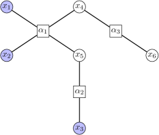
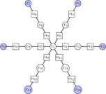
Figure 2 depicts a factor graph with leaf nodes L={1,2,3,6}𝐿1236L=\{1,2,3,6\}. The shaded nodes in the figure represent the fixed distribution variables, thus, in this example, Γ={1,2,3}LΓ123𝐿\Gamma=\{1,2,3\}\subset L.

Refer to caption
Figure 2: Factor graph with some marginal distribution constraints on nodes {x1,x2,x3}subscript𝑥1subscript𝑥2subscript𝑥3\{x_{1},x_{2},x_{3}\}.

Leveraging the graphical structure (30) of the cost, based on the discussions above, we obtain a simple strategy to solve the MOT problem (23): We apply the Iterative Scaling algorithm and utilize the Belief Propagation algorithm to carry out the computation of Pj(𝐊𝐔)subscript𝑃𝑗direct-product𝐊𝐔P_{j}({\bf K}\odot{\bf U}) with the current multiplier 𝐔𝐔{\bf U}. The acceleration is tremendous for MOT problems with a large number of marginals; the Belief Propagation algorithm scales well for large problem while the complexity of the brute force projection using definition (21) grows exponentially as the dimension increases. It turns out that some more tricks can be adopted to further improve the speed of the projection step Pj(𝐊𝐔)subscript𝑃𝑗direct-product𝐊𝐔P_{j}({\bf K}\odot{\bf U}). The full algorithm, which we call Iterative Scaling Belief Propagation (ISBP) algorithm will be presented and discussed in details in Section III-D.

III-C MOT and Bayesian inference

In the previous section, we have seen that in cases where the cost tensor 𝐂𝐂{\bf C} in MOT problem (23) has a graphical structure, one can take advantage of PGM methods, in particular the Belief Propagation algorithm, to accelerate the Iterative Scaling algorithm. In this section, we establish further connections between MOT and PGMs. These links add novel components to both the MOT theory and PGM theory. These connections also bring new insight and interpretation of Iterative Scaling Belief Propagation.

Clearly, the objective function of the entropy regularized MOT problem (23) is exactly the free energy {\mathcal{F}} in (12) with

ψα(𝐱α)=exp(Cα(𝐱α)),αF,𝐱αϕj(xj)=1,jV,xj.formulae-sequencesubscript𝜓𝛼subscript𝐱𝛼subscript𝐶𝛼subscript𝐱𝛼formulae-sequencefor-all𝛼𝐹for-allsubscript𝐱𝛼formulae-sequencesubscriptitalic-ϕ𝑗subscript𝑥𝑗1for-all𝑗𝑉for-allsubscript𝑥𝑗\psi_{\alpha}({\mathbf{x}}_{\alpha})=\exp(-C_{\alpha}({\mathbf{x}}_{\alpha})),\ \forall\alpha\in F,\forall{\mathbf{x}}_{\alpha}\qquad\phi_{j}(x_{j})=1,\ \forall j\in V,\forall x_{j}. (33)

Thus, the MOT problem (23) can be written as

min𝐁+d1××dJsubscript𝐁superscriptsubscriptsubscript𝑑1subscript𝑑𝐽\displaystyle\min_{{\mathbf{B}}\in{\mathbb{R}}_{+}^{d_{1}\times\dots\times d_{J}}} (𝐁)𝐁\displaystyle~{}{\mathcal{F}}({\mathbf{B}}) (34)
subject to Pj(𝐁)=𝝁j,jΓ.formulae-sequencesubscript𝑃𝑗𝐁subscript𝝁𝑗for-all𝑗Γ\displaystyle~{}P_{j}({\mathbf{B}})=\boldsymbol{\mu}_{j},\quad\forall j\in\Gamma.

Therefore, the entropic regularized MOT problem (23) with cost function that decouples according to a graph structure as in (30) is equivalent to a Bayesian inference problem in a PGM with additional constraints on the marginal distributions of a set of variable nodes. In other words, (34) is a constrained version of a Bayesian inference problem.

On the other hand, any Bayesian inference problem in a PGM can be rewritten in the constrained form (34). More specifically, consider the problem of inferring the posterior distribution of

1ZjΓϕj(xj,yj)αFψα(𝐱α),1𝑍subscriptproduct𝑗Γsubscriptitalic-ϕ𝑗subscript𝑥𝑗subscript𝑦𝑗subscriptproduct𝛼𝐹subscript𝜓𝛼subscript𝐱𝛼\frac{1}{Z}\prod_{j\in\Gamma}\phi_{j}(x_{j},y_{j})\prod_{\alpha\in F}\psi_{\alpha}(\mathbf{x}_{\alpha}),

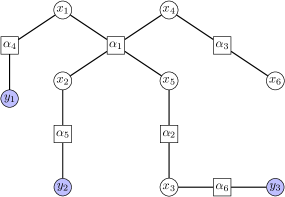
where yjsubscript𝑦𝑗y_{j} is the observation associated with the variable node potential ϕjsubscriptitalic-ϕ𝑗\phi_{j}. When the observations are fixed, say yj=y^jsubscript𝑦𝑗subscript^𝑦𝑗y_{j}=\hat{y}_{j}, then the standard Bayesian inference method replaces ϕj(xj,yj)subscriptitalic-ϕ𝑗subscript𝑥𝑗subscript𝑦𝑗\phi_{j}(x_{j},y_{j}) by a local potential ϕj(xj)subscriptitalic-ϕ𝑗subscript𝑥𝑗\phi_{j}(x_{j}) and infers the marginal distributions of the resulting graphical model with only the nodes {xj,𝐱α}subscript𝑥𝑗subscript𝐱𝛼\{x_{j},\,{\mathbf{x}}_{\alpha}\}. Alternatively, the measurement yj=y^jsubscript𝑦𝑗subscript^𝑦𝑗y_{j}=\hat{y}_{j} can be viewed as constraints on the node yjsubscript𝑦𝑗y_{j} of an augmented graphical model which includes also the observation variable node yjsubscript𝑦𝑗y_{j}. In particular, the constraint is of the form p(yj)=δ(yjy^j)𝑝subscript𝑦𝑗𝛿subscript𝑦𝑗subscript^𝑦𝑗p(y_{j})=\delta(y_{j}-\hat{y}_{j}), where δ𝛿\delta denotes Dirac distribution. Thus, the posterior distribution can also be obtained by solving the constrained Bayesian inference problem (34) over the augmented graphical models under the constraints that p(yj)=δ(yjy^j)𝑝subscript𝑦𝑗𝛿subscript𝑦𝑗subscript^𝑦𝑗p(y_{j})=\delta(y_{j}-\hat{y}_{j}), for jΓ𝑗Γj\in\Gamma. This equivalence is illustrated in Figure 3. Therefore, from this point of view, the constrained Bayesian inference problem (34) can also be viewed as a generalization of standard Bayesian inference.
Refer to caption
(a) Standard
Refer to caption
(b) Constrained
Figure 3: Equivalence between standard Bayesian inference and constrained Bayesian inference: (a) The local potentials of variables x1,x2,x3subscript𝑥1subscript𝑥2subscript𝑥3x_{1},~{}x_{2},~{}x_{3} are induced by measurements y1=y^1,y2=y^2,y3=y^3formulae-sequencesubscript𝑦1subscript^𝑦1formulae-sequencesubscript𝑦2subscript^𝑦2subscript𝑦3subscript^𝑦3y_{1}=\hat{y}_{1},~{}y_{2}=\hat{y}_{2},~{}y_{3}=\hat{y}_{3} respectively, namely, ϕ1(x1)=ϕ1(x1,y^1),ϕ2(x2)=ϕ2(x2,y^2),ϕ3(x3)=ϕ3(x3,y^3)formulae-sequencesubscriptitalic-ϕ1subscript𝑥1subscriptitalic-ϕ1subscript𝑥1subscript^𝑦1formulae-sequencesubscriptitalic-ϕ2subscript𝑥2subscriptitalic-ϕ2subscript𝑥2subscript^𝑦2subscriptitalic-ϕ3subscript𝑥3subscriptitalic-ϕ3subscript𝑥3subscript^𝑦3\phi_{1}(x_{1})=\phi_{1}(x_{1},\hat{y}_{1}),~{}\phi_{2}(x_{2})=\phi_{2}(x_{2},\hat{y}_{2}),~{}\phi_{3}(x_{3})=\phi_{3}(x_{3},\hat{y}_{3}); (b) The graph is augmented by the nodes y1,y2,y3subscript𝑦1subscript𝑦2subscript𝑦3y_{1},~{}y_{2},~{}y_{3} and factors ψα4=ϕ1(x1,y1)subscript𝜓subscript𝛼4subscriptitalic-ϕ1subscript𝑥1subscript𝑦1\psi_{\alpha_{4}}=\phi_{1}(x_{1},y_{1}), ψα5=ϕ2(x2,y2)subscript𝜓subscript𝛼5subscriptitalic-ϕ2subscript𝑥2subscript𝑦2\psi_{\alpha_{5}}=\phi_{2}(x_{2},y_{2}), and ψα6=ϕ3(x3,y3)subscript𝜓subscript𝛼6subscriptitalic-ϕ3subscript𝑥3subscript𝑦3\psi_{\alpha_{6}}=\phi_{3}(x_{3},y_{3}). The measurements become marginal constraints p(y1)=δ(y1y^1),p(y2)=δ(y2y^2),p(y3)=δ(y3y^3)formulae-sequence𝑝subscript𝑦1𝛿subscript𝑦1subscript^𝑦1formulae-sequence𝑝subscript𝑦2𝛿subscript𝑦2subscript^𝑦2𝑝subscript𝑦3𝛿subscript𝑦3subscript^𝑦3p(y_{1})=\delta(y_{1}-\hat{y}_{1}),~{}p(y_{2})=\delta(y_{2}-\hat{y}_{2}),~{}p(y_{3})=\delta(y_{3}-\hat{y}_{3}).

When the underlying factor graph associated with the cost function (30) is in fact a factor tree, the free energy (𝐁)𝐁{\mathcal{F}}({\mathbf{B}}) is equal to the Bethe free energy (see Section II-C)

Bethe(𝐁)=αF𝐱αBα(𝐱α)lnψα(𝐱α)+ϵαF𝐱αBα(𝐱α)lnBα(𝐱α)ϵjV(Nj1)xjBj(xj)lnBj(xj),subscriptBethe𝐁subscript𝛼𝐹subscriptsubscript𝐱𝛼subscript𝐵𝛼subscript𝐱𝛼subscript𝜓𝛼subscript𝐱𝛼italic-ϵsubscript𝛼𝐹subscriptsubscript𝐱𝛼subscript𝐵𝛼subscript𝐱𝛼subscript𝐵𝛼subscript𝐱𝛼italic-ϵsubscript𝑗𝑉subscript𝑁𝑗1subscriptsubscript𝑥𝑗subscript𝐵𝑗subscript𝑥𝑗subscript𝐵𝑗subscript𝑥𝑗{\mathcal{F}}_{\rm Bethe}({\mathbf{B}})=-\sum_{\alpha\in F}\sum_{{\bf x}_{\alpha}}B_{\alpha}({\bf x}_{\alpha})\ln\psi_{\alpha}({\bf x}_{\alpha})+\epsilon\,\sum_{\alpha\in F}\sum_{{\bf x}_{\alpha}}B_{\alpha}({\bf x}_{\alpha})\ln B_{\alpha}({\bf x}_{\alpha})-\epsilon\,\sum_{j\in V}(N_{j}-1)\sum_{x_{j}}B_{j}(x_{j})\ln B_{j}(x_{j}), (35)

where 𝐁αsubscript𝐁𝛼{\mathbf{B}}_{\alpha} is the marginal distribution on factor node α𝛼\alpha and 𝐁jsubscript𝐁𝑗{\mathbf{B}}_{j} denotes the marginal on variable node j𝑗j, namely, Bα(𝐱α)=𝐱\𝐱αB(𝐱)subscript𝐵𝛼subscript𝐱𝛼subscript\𝐱subscript𝐱𝛼𝐵𝐱B_{\alpha}({\mathbf{x}}_{\alpha})=\sum_{{\mathbf{x}}\backslash{\mathbf{x}}_{\alpha}}B({\mathbf{x}}), and Bj(xj)=𝐱\xjB(𝐱)subscript𝐵𝑗subscript𝑥𝑗subscript\𝐱subscript𝑥𝑗𝐵𝐱B_{j}(x_{j})=\sum_{{\mathbf{x}}\backslash x_{j}}B({\mathbf{x}}). In (35), 𝐁𝐁{\mathbf{B}} is the collection of marginal distributions, that is, 𝐁={𝐁j,𝐁α:jV,αF}𝐁conditional-setsubscript𝐁𝑗subscript𝐁𝛼formulae-sequence𝑗𝑉𝛼𝐹{\mathbf{B}}=\{{\mathbf{B}}_{j},{\mathbf{B}}_{\alpha}~{}:~{}j\in V,\alpha\in F\}. This is different from the J𝐽J-mode tensor 𝐁𝐁{\mathbf{B}} in (34). However, with slight abuse of notation, we use the same symbol 𝐁𝐁{\mathbf{B}} in both contexts. Again, due to tree structure, the two have a one-to-one correspondence with each other.

The marginals 𝐁αsubscript𝐁𝛼{\mathbf{B}}_{\alpha} and 𝐁jsubscript𝐁𝑗{\mathbf{B}}_{j} capture only local information around a factor variable or node variable and they have to satisfy certain conditions in order to be feasible marginal distributions of some joint distribution. In particular, they have to be compatible in the sense

𝐱α\xjBα(𝐱α)=Bj(xj),jV,xj.formulae-sequencesubscript\subscript𝐱𝛼subscript𝑥𝑗subscript𝐵𝛼subscript𝐱𝛼subscript𝐵𝑗subscript𝑥𝑗for-all𝑗𝑉for-allsubscript𝑥𝑗\sum_{{\bf x}_{\alpha}\backslash x_{j}}B_{\alpha}({\bf x}_{\alpha})=B_{j}(x_{j}),\quad\forall j\in V,\,\forall x_{j}.

In terms of local marginals, the constraints in (34) read

Bj(xj)=μj(xj),jΓ,xj.formulae-sequencesubscript𝐵𝑗subscript𝑥𝑗subscript𝜇𝑗subscript𝑥𝑗for-all𝑗Γfor-allsubscript𝑥𝑗B_{j}(x_{j})=\mu_{j}(x_{j}),\quad\forall j\in\Gamma,\,\forall x_{j}.

Therefore, the MOT problem (34) can be reformulated as

min𝐁subscript𝐁\displaystyle\min_{{\mathbf{B}}} Bethe(𝐁)subscriptBethe𝐁\displaystyle{\mathcal{F}}_{\rm Bethe}({\mathbf{B}}) (36a)
subject to Bj(xj)=μj(xj),jΓ,xjformulae-sequencesubscript𝐵𝑗subscript𝑥𝑗subscript𝜇𝑗subscript𝑥𝑗for-all𝑗Γfor-allsubscript𝑥𝑗\displaystyle B_{j}(x_{j})=\mu_{j}(x_{j}),\quad\forall j\in\Gamma,~{}\forall x_{j} (36d)
𝐱α\xjBα(𝐱α)=Bj(xj),jV,αN(j),xjformulae-sequencesubscript\subscript𝐱𝛼subscript𝑥𝑗subscript𝐵𝛼subscript𝐱𝛼subscript𝐵𝑗subscript𝑥𝑗formulae-sequencefor-all𝑗𝑉𝛼𝑁𝑗for-allsubscript𝑥𝑗\displaystyle\sum_{{\bf x}_{\alpha}\backslash x_{j}}B_{\alpha}({\bf x}_{\alpha})=B_{j}(x_{j}),\quad\forall j\in V,\alpha\in N(j),~{}\forall x_{j}
𝐱αBα(𝐱α)=1,αF,formulae-sequencesubscriptsubscript𝐱𝛼subscript𝐵𝛼subscript𝐱𝛼1for-all𝛼𝐹\displaystyle\sum_{{\bf x}_{\alpha}}B_{\alpha}({\bf x}_{\alpha})=1,\quad\forall\alpha\in F,

where the last constraint (36d) is to ensure that the optimization variables {𝐁j,𝐁α:jV,αF}conditional-setsubscript𝐁𝑗subscript𝐁𝛼formulae-sequence𝑗𝑉𝛼𝐹\{{\mathbf{B}}_{j},{\mathbf{B}}_{\alpha}~{}:~{}j\in V,\alpha\in F\} are in the probability simplex. Since the Bethe free energy is convex for factor trees, and the constraints are linear, Problem (36) is a convex optimization problem. One advantage of (36) over (34) is that the size of optimization variables in (36) is considerably smaller than that in (34). More specifically, the optimization variables of (36) are local marginals which are either vectors 𝐁jsubscript𝐁𝑗{\mathbf{B}}_{j} or low-dimensional tensors 𝐁αsubscript𝐁𝛼{\mathbf{B}}_{\alpha}, which is in contrast to the high-dimensional J𝐽J-mode tensor 𝐁𝐁{\mathbf{B}} in (34).

III-D Iterative Scaling Belief Propagation algorithm

In this section, we present the full Iterative Scaling Belief Propagation algorithm for the entropy regularized MOT problem (23) (or equivalently (34) and (36)). We start with a characterization of the solution to (36).

Theorem 3.

The solution to the MOT problem (36) is given by

Bα(𝐱α)subscript𝐵𝛼subscript𝐱𝛼\displaystyle B_{\alpha}({\bf x}_{\alpha}) proportional-to\displaystyle\propto Kα(𝐱α)jN(α)njα(xj),αFsubscript𝐾𝛼subscript𝐱𝛼subscriptproduct𝑗𝑁𝛼subscript𝑛𝑗𝛼subscript𝑥𝑗for-all𝛼𝐹\displaystyle K_{\alpha}({\bf x}_{\alpha})\prod_{j\in N(\alpha)}n_{j\rightarrow\alpha}(x_{j}),\quad\forall\alpha\in F (37a)
Bj(xj)subscript𝐵𝑗subscript𝑥𝑗\displaystyle B_{j}(x_{j}) proportional-to\displaystyle\propto αN(j)mαj(xj),jΓsubscriptproduct𝛼𝑁𝑗subscript𝑚𝛼𝑗subscript𝑥𝑗for-all𝑗Γ\displaystyle\prod_{\alpha\in N(j)}m_{\alpha\rightarrow j}(x_{j}),~{}\forall j\notin\Gamma (37b)
Bj(xj)subscript𝐵𝑗subscript𝑥𝑗\displaystyle B_{j}(x_{j}) =\displaystyle= μj(xj),jΓsubscript𝜇𝑗subscript𝑥𝑗for-all𝑗Γ\displaystyle\mu_{j}(x_{j}),~{}\forall j\in\Gamma (37c)

where mαj,njαsubscript𝑚𝛼𝑗subscript𝑛𝑗𝛼m_{\alpha\rightarrow j},\,n_{j\rightarrow\alpha} are fixed points of the following iterations

mαj(xj)subscript𝑚𝛼𝑗subscript𝑥𝑗\displaystyle m_{\alpha\rightarrow j}(x_{j}) proportional-to\displaystyle\propto 𝐱α\xjKα(𝐱α)iN(α)\jniα(xi);jV,αN(j),xj,formulae-sequencesubscript\subscript𝐱𝛼subscript𝑥𝑗subscript𝐾𝛼subscript𝐱𝛼subscriptproduct𝑖\𝑁𝛼𝑗subscript𝑛𝑖𝛼subscript𝑥𝑖for-all𝑗𝑉for-all𝛼𝑁𝑗for-allsubscript𝑥𝑗\displaystyle\sum_{{\bf x}_{\alpha}\backslash x_{j}}K_{\alpha}({\bf x}_{\alpha})\prod_{i\in N(\alpha)\backslash j}n_{i\rightarrow\alpha}(x_{i});\quad\forall j\in V,~{}\forall\alpha\in N(j),~{}\forall x_{j}, (38a)
njα(xj)subscript𝑛𝑗𝛼subscript𝑥𝑗\displaystyle n_{j\rightarrow\alpha}(x_{j}) proportional-to\displaystyle\propto βN(j)\αmβj(xj);jΓ,αN(j),xj,formulae-sequencesubscriptproduct𝛽\𝑁𝑗𝛼subscript𝑚𝛽𝑗subscript𝑥𝑗for-all𝑗Γfor-all𝛼𝑁𝑗for-allsubscript𝑥𝑗\displaystyle\prod_{\beta\in N(j)\backslash\alpha}m_{\beta\rightarrow j}(x_{j});\quad\forall j\notin\Gamma,~{}\forall\alpha\in N(j),~{}\forall x_{j}, (38b)
njα(xj)subscript𝑛𝑗𝛼subscript𝑥𝑗\displaystyle n_{j\rightarrow\alpha}(x_{j}) proportional-to\displaystyle\propto μj(xj)(mαj(xj))1;jΓ,xj.formulae-sequencesubscript𝜇𝑗subscript𝑥𝑗superscriptsubscript𝑚𝛼𝑗subscript𝑥𝑗1for-all𝑗Γfor-allsubscript𝑥𝑗\displaystyle\mu_{j}(x_{j})(m_{\alpha\rightarrow j}(x_{j}))^{-1};\quad\forall j\in\Gamma,~{}\forall x_{j}. (38c)

Here proportional-to\propto indicates that a normalization step is needed.

Proof.

In order to solve the constrained optimization problem (36), we introduce Lagrange multipliers ηαsubscript𝜂𝛼\eta_{\alpha} for the simplex constraints (36d), 𝝀j,αsubscript𝝀𝑗𝛼\boldsymbol{\lambda}_{j,\alpha} for the marginalization compatibility constraints (36d), and 𝝂jsubscript𝝂𝑗\boldsymbol{\nu}_{j} for the fixed-marginal constraints (36d), yielding the Lagrangian

=1ϵBethe(𝐁)+αηα(𝐱αBα(𝐱α)1)+j,xjαN(j)λj,α(xj)(𝐱α\xjBα(𝐱α)Bj(xj))+jΓxjνj(xj)(Bj(xj)μj(xj)).1italic-ϵsubscriptBethe𝐁subscript𝛼subscript𝜂𝛼subscriptsubscript𝐱𝛼subscript𝐵𝛼subscript𝐱𝛼1subscript𝑗subscript𝑥𝑗subscript𝛼𝑁𝑗subscript𝜆𝑗𝛼subscript𝑥𝑗subscript\subscript𝐱𝛼subscript𝑥𝑗subscript𝐵𝛼subscript𝐱𝛼subscript𝐵𝑗subscript𝑥𝑗subscript𝑗Γsubscriptsubscript𝑥𝑗subscript𝜈𝑗subscript𝑥𝑗subscript𝐵𝑗subscript𝑥𝑗subscript𝜇𝑗subscript𝑥𝑗{\mathcal{L}}=\frac{1}{\epsilon}{\mathcal{F}}_{\rm Bethe}({\mathbf{B}})+\sum_{\alpha}\eta_{\alpha}\left(\sum_{{\bf x}_{\alpha}}B_{\alpha}({\bf x}_{\alpha})-1\right)+\sum_{j,x_{j}}\sum_{\alpha\in N(j)}\lambda_{j,\alpha}(x_{j})\left(\sum_{{\mathbf{x}}_{\alpha}\backslash x_{j}}B_{\alpha}({\bf x}_{\alpha})-B_{j}(x_{j})\right)+\sum_{j\in\Gamma}\sum_{x_{j}}\nu_{j}(x_{j})\left(B_{j}(x_{j})-\mu_{j}(x_{j})\right). (39)

Note that we have used a scaled version 1ϵBethe1italic-ϵsubscriptBethe\frac{1}{\epsilon}{\mathcal{F}}_{\rm Bethe} of the objective function. In view of (33), (35) and (31),

1ϵBethe(𝐁)=αF𝐱αBα(𝐱α)lnKα(𝐱α)+αF𝐱αBα(𝐱α)lnBα(𝐱α)jV(Nj1)xjBj(xj)lnBj(xj).1italic-ϵsubscriptBethe𝐁subscript𝛼𝐹subscriptsubscript𝐱𝛼subscript𝐵𝛼subscript𝐱𝛼subscript𝐾𝛼subscript𝐱𝛼subscript𝛼𝐹subscriptsubscript𝐱𝛼subscript𝐵𝛼subscript𝐱𝛼subscript𝐵𝛼subscript𝐱𝛼subscript𝑗𝑉subscript𝑁𝑗1subscriptsubscript𝑥𝑗subscript𝐵𝑗subscript𝑥𝑗subscript𝐵𝑗subscript𝑥𝑗\frac{1}{\epsilon}{\mathcal{F}}_{\rm Bethe}({\mathbf{B}})=-\sum_{\alpha\in F}\sum_{{\bf x}_{\alpha}}B_{\alpha}({\bf x}_{\alpha})\ln K_{\alpha}({\bf x}_{\alpha})+\sum_{\alpha\in F}\sum_{{\bf x}_{\alpha}}B_{\alpha}({\bf x}_{\alpha})\ln B_{\alpha}({\bf x}_{\alpha})-\sum_{j\in V}(N_{j}-1)\sum_{x_{j}}B_{j}(x_{j})\ln B_{j}(x_{j}).

Setting the derivatives of the Lagrangian with respect to the local marginals 𝐁αsubscript𝐁𝛼{\mathbf{B}}_{\alpha} and 𝐁jsubscript𝐁𝑗{\mathbf{B}}_{j} to zero, we get that the minimizer satisfies

Bα(𝐱α)subscript𝐵𝛼subscript𝐱𝛼\displaystyle B_{\alpha}({\bf x}_{\alpha}) =\displaystyle= Kα(𝐱α)exp(1jN(α)λj,α(xj)ηα),subscript𝐾𝛼subscript𝐱𝛼1subscript𝑗𝑁𝛼subscript𝜆𝑗𝛼subscript𝑥𝑗subscript𝜂𝛼\displaystyle K_{\alpha}({\bf x}_{\alpha})~{}\exp\left(-1-\sum_{j\in N(\alpha)}\lambda_{j,\alpha}(x_{j})-\eta_{\alpha}\right), (40a)
Bj(xj)subscript𝐵𝑗subscript𝑥𝑗\displaystyle B_{j}(x_{j}) =\displaystyle= exp(11Nj1αN(j)λj,α(xj))ifNj>111subscript𝑁𝑗1subscript𝛼𝑁𝑗subscript𝜆𝑗𝛼subscript𝑥𝑗ifsubscript𝑁𝑗1\displaystyle\exp\left(-1-\frac{1}{N_{j}-1}\sum_{\alpha\in N(j)}\lambda_{j,\alpha}(x_{j})\right)\quad~{}\mbox{if}~{}N_{j}>1 (40b)
00\displaystyle 0 =\displaystyle= αN(j)λj,α(xj)ifNj=1,jΓformulae-sequencesubscript𝛼𝑁𝑗subscript𝜆𝑗𝛼subscript𝑥𝑗ifsubscript𝑁𝑗1𝑗Γ\displaystyle\sum_{\alpha\in N(j)}\lambda_{j,\alpha}(x_{j})\quad~{}\mbox{if}~{}N_{j}=1,j\notin\Gamma (40c)
00\displaystyle 0 =\displaystyle= αN(j)λj,α(xj)νj(xj)ifjΓsubscript𝛼𝑁𝑗subscript𝜆𝑗𝛼subscript𝑥𝑗subscript𝜈𝑗subscript𝑥𝑗if𝑗Γ\displaystyle\sum_{\alpha\in N(j)}\lambda_{j,\alpha}(x_{j})-\nu_{j}(x_{j})\quad~{}\mbox{if}~{}j\in\Gamma (40d)

Denote

njα(xj)subscript𝑛𝑗𝛼subscript𝑥𝑗\displaystyle n_{j\rightarrow\alpha}(x_{j}) :=assign\displaystyle:= exp(λj,α(xj))subscript𝜆𝑗𝛼subscript𝑥𝑗\displaystyle\exp(-\lambda_{j,\alpha}(x_{j})) (41a)
mαj(xj)subscript𝑚𝛼𝑗subscript𝑥𝑗\displaystyle m_{\alpha\rightarrow j}(x_{j}) :=assign\displaystyle:= 𝐱α\xjKα(𝐱α)iN(α)\jniα(xi).subscript\subscript𝐱𝛼subscript𝑥𝑗subscript𝐾𝛼subscript𝐱𝛼subscriptproduct𝑖\𝑁𝛼𝑗subscript𝑛𝑖𝛼subscript𝑥𝑖\displaystyle\sum_{{\mathbf{x}}_{\alpha}\backslash x_{j}}K_{\alpha}({\mathbf{x}}_{\alpha})\prod_{i\in N(\alpha)\backslash j}n_{i\rightarrow\alpha}(x_{i}). (41b)

The relation (37a) follows immediately from (40a) and (41a). This together with the constraint (36d) and (41b) leads to

Bj(xj)=𝐱α\xjBα(𝐱α)njα(xj)mαj(xj).subscript𝐵𝑗subscript𝑥𝑗subscript\subscript𝐱𝛼subscript𝑥𝑗subscript𝐵𝛼subscript𝐱𝛼proportional-tosubscript𝑛𝑗𝛼subscript𝑥𝑗subscript𝑚𝛼𝑗subscript𝑥𝑗B_{j}(x_{j})=\sum_{{\bf x}_{\alpha}\backslash x_{j}}B_{\alpha}({\bf x}_{\alpha})\propto n_{j\rightarrow\alpha}(x_{j})m_{\alpha\rightarrow j}(x_{j}). (42)

By (40c), we obtain

njα(xj)=1ifNj=1,jΓ.formulae-sequencesubscript𝑛𝑗𝛼subscript𝑥𝑗1ifsubscript𝑁𝑗1𝑗Γn_{j\rightarrow\alpha}(x_{j})=1~{}\mbox{if}~{}N_{j}=1,j\notin\Gamma.

It follows that

Bj(xj)mαj(xj)ifNj=1,jΓ,formulae-sequenceproportional-tosubscript𝐵𝑗subscript𝑥𝑗subscript𝑚𝛼𝑗subscript𝑥𝑗ifsubscript𝑁𝑗1𝑗ΓB_{j}(x_{j})\propto m_{\alpha\rightarrow j}(x_{j})~{}\mbox{if}~{}N_{j}=1,j\notin\Gamma,

which is (37b) for leaf nodes. We next show (37b) when Nj>1subscript𝑁𝑗1N_{j}>1. To this end, we plug (40a) and (40b) into the constraint (36d) and arrive at

njγ(xj)mγj(xj)subscript𝑛𝑗𝛾subscript𝑥𝑗subscript𝑚𝛾𝑗subscript𝑥𝑗\displaystyle n_{j\rightarrow\gamma}(x_{j})m_{\gamma\rightarrow j}(x_{j}) proportional-to\displaystyle\propto 𝐱γ\xjBγ(𝐱γ)subscript\subscript𝐱𝛾subscript𝑥𝑗subscript𝐵𝛾subscript𝐱𝛾\displaystyle\sum_{{\bf x}_{\gamma}\backslash x_{j}}B_{\gamma}({\bf x}_{\gamma})
=\displaystyle= Bj(xj)exp(11Nj1βN(j)λj,β(xj))proportional-tosubscript𝐵𝑗subscript𝑥𝑗11subscript𝑁𝑗1subscript𝛽𝑁𝑗subscript𝜆𝑗𝛽subscript𝑥𝑗\displaystyle B_{j}(x_{j})\propto\exp\left(-1-\frac{1}{N_{j}-1}\sum_{\beta\in N(j)}\lambda_{j,\beta}(x_{j})\right)
proportional-to\displaystyle\propto βN(j)njβ(xj)1Nj1.subscriptproduct𝛽𝑁𝑗subscript𝑛𝑗𝛽superscriptsubscript𝑥𝑗1subscript𝑁𝑗1\displaystyle\prod_{\beta\in N(j)}n_{j\rightarrow\beta}(x_{j})^{\frac{1}{N_{j}-1}}.

For fixed j𝑗j, the above holds for all γN(j)𝛾𝑁𝑗\gamma\in N(j). Multiplying the above equation for all γN(j)\α𝛾\𝑁𝑗𝛼\gamma\in N(j)\backslash\alpha yields

γN(j)\α(njγ(xj)mγj(xj))βN(j)njβ(xj),proportional-tosubscriptproduct𝛾\𝑁𝑗𝛼subscript𝑛𝑗𝛾subscript𝑥𝑗subscript𝑚𝛾𝑗subscript𝑥𝑗subscriptproduct𝛽𝑁𝑗subscript𝑛𝑗𝛽subscript𝑥𝑗\prod_{\gamma\in N(j)\backslash\alpha}\left(n_{j\rightarrow\gamma}(x_{j})m_{\gamma\rightarrow j}(x_{j})\right)\propto\prod_{\beta\in N(j)}n_{j\rightarrow\beta}(x_{j}),

which is (38b) after canceling out equal terms. Thus, in view of (42),

Bj(xj)njα(xj)mαj(xj)αN(j)mαj(xj),ifNj>1.formulae-sequenceproportional-tosubscript𝐵𝑗subscript𝑥𝑗subscript𝑛𝑗𝛼subscript𝑥𝑗subscript𝑚𝛼𝑗subscript𝑥𝑗proportional-tosubscriptproduct𝛼𝑁𝑗subscript𝑚𝛼𝑗subscript𝑥𝑗ifsubscript𝑁𝑗1B_{j}(x_{j})\propto n_{j\rightarrow\alpha}(x_{j})m_{\alpha\rightarrow j}(x_{j})\propto\prod_{\alpha\in N(j)}m_{\alpha\rightarrow j}(x_{j}),~{}\mbox{if}~{}N_{j}>1.

Finally, (37c) is clearly true due to constraints. This together with (42) leads to (38c), which completes the proof. ∎

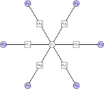
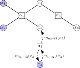
The updates in (38) resemble the standard Belief Propagation algorithm (13). In particular, the updates (38a) and (38b) are exactly the same as (13). The update (38c) is new and is due to the constraints (36d) on the marginal distributions. Pictorially the message 𝐦αjsubscript𝐦𝛼𝑗{\mathbf{m}}_{\alpha\rightarrow j} sent to a constrained node j𝑗j from node α𝛼\alpha bounces back to α𝛼\alpha, in form of 𝐧jαsubscript𝐧𝑗𝛼{\mathbf{n}}_{j\rightarrow\alpha}. This is illustrated in Figure 4. The update (38c) in fact corresponds to the scaling step (29) of the Iterative Scaling algorithm (Algorithm 1). In particular, the multipliers {𝐮j:jΓ}conditional-setsubscript𝐮𝑗𝑗Γ\{{\mathbf{u}}_{j}~{}:~{}j\in\Gamma\} in (27) relate to the messages as 𝐮j=𝐧jαsubscript𝐮𝑗subscript𝐧𝑗𝛼{\mathbf{u}}_{j}={\mathbf{n}}_{j\rightarrow\alpha}, for jΓ𝑗Γj\in\Gamma. To see this, we note that the projection Pj(𝐊𝐔)subscript𝑃𝑗direct-product𝐊𝐔P_{j}({\bf K}\odot{\bf U}) requires solving a Bayesian inference problem with respect to the modified graphical model

p(𝐱)=1ZαFKα(𝐱α)jΓuj(xj).𝑝𝐱1𝑍subscriptproduct𝛼𝐹subscript𝐾𝛼subscript𝐱𝛼subscriptproduct𝑗Γsubscript𝑢𝑗subscript𝑥𝑗p({\mathbf{x}})=\frac{1}{Z}\prod_{\alpha\in F}K_{\alpha}({\mathbf{x}}_{\alpha})\prod_{j\in\Gamma}u_{j}(x_{j}). (43)

Upon convergence of the Belief Propagation algorithm (13), it holds Pj(𝐊𝐔)=𝐮j𝐦αjsubscript𝑃𝑗direct-product𝐊𝐔subscript𝐮𝑗subscript𝐦𝛼𝑗P_{j}({\bf K}\odot{\bf U})={\mathbf{u}}_{j}{\mathbf{m}}_{\alpha\rightarrow j}, where α𝛼\alpha is the only factor node in N(j)𝑁𝑗N(j) since jΓ𝑗Γj\in\Gamma is a leaf node. Thus, the projection step (29) reads
𝐮j𝝁j./Pj(𝐊𝐔)=𝝁j./𝐦αj=𝐧jα.{\mathbf{u}}_{j}\odot\boldsymbol{\mu}_{j}./P_{j}({\bf K}\odot{\bf U})=\boldsymbol{\mu}_{j}./{\mathbf{m}}_{\alpha\rightarrow j}={\mathbf{n}}_{j\rightarrow\alpha}.
Refer to caption
Figure 4: Messages in ISBP

Therefore, the updates (38) contain all the components of our ISBP algorithm with (38a)-(38b) being the Belief Propagation part and (38c) being the Iterative Scaling part. ISBP is a scheduling of these updates in a certain order. As discussed in Section III-B, the key idea of ISBP is to implement the projection Pj(𝐊𝐔)subscript𝑃𝑗direct-product𝐊𝐔P_{j}({\bf K}\odot{\bf U}) in the iterative scaling step (29) using Belief Propagation. In the contexts of the updates (38), it is equivalent to run (38a)-(38b) sufficiently many iterations to obtain the precise projection Pj(𝐊𝐔)subscript𝑃𝑗direct-product𝐊𝐔P_{j}({\bf K}\odot{\bf U}) and then run (38c), which is essentially (29). How many iterations of (38a)-(38b) are enough? One option is to run Belief Propagation over the whole graph G𝐺G with the most recent modified model 𝐊𝐔direct-product𝐊𝐔{\bf K}\odot{\bf U} to compute Pj(𝐊𝐔)subscript𝑃𝑗direct-product𝐊𝐔P_{j}({\bf K}\odot{\bf U}) for all jV𝑗𝑉j\in V. This is clearly sufficient but it is not necessary. Let j1,j2,subscript𝑗1subscript𝑗2j_{1},j_{2},\ldots be a sequence taking values in ΓΓ\Gamma in arbitrary order and suppose the Iterative Scaling algorithm is carried out in this order. Then after the k𝑘k-th step, 𝐮jksubscript𝐮subscript𝑗𝑘{\mathbf{u}}_{j_{k}} is updated, and the only projection required in the next step is Pjk+1(𝐊𝐔)subscript𝑃subscript𝑗𝑘1direct-product𝐊𝐔P_{j_{k+1}}({\bf K}\odot{\bf U}). It turns out that to evaluate Pjk+1(𝐊𝐔)subscript𝑃subscript𝑗𝑘1direct-product𝐊𝐔P_{j_{k+1}}({\bf K}\odot{\bf U}), it suffices to update all the messages on the path from jksubscript𝑗𝑘j_{k} to jk+1subscript𝑗𝑘1j_{k+1}. Compared to the naive Belief Propagation over the whole graph, this local updating strategy is considerably faster. The steps of the ISBP algorithm are summarized in Algorithm 2.

Algorithm 2 Iterative Scaling Belief Propagation (ISBP) Algorithm for MOT
  Initialize the messages mαj(xj)subscript𝑚𝛼𝑗subscript𝑥𝑗m_{\alpha\rightarrow j}(x_{j}) and njα(xj)subscript𝑛𝑗𝛼subscript𝑥𝑗n_{j\rightarrow\alpha}(x_{j})
  Update mαj(xj)subscript𝑚𝛼𝑗subscript𝑥𝑗m_{\alpha\rightarrow j}(x_{j}) and njα(xj)subscript𝑛𝑗𝛼subscript𝑥𝑗n_{j\rightarrow\alpha}(x_{j}) using (38a)-(38b) until convergence
  while not converged do
     Update njkα(xjk)subscript𝑛subscript𝑗𝑘𝛼subscript𝑥subscript𝑗𝑘n_{j_{k}\rightarrow\alpha}(x_{j_{k}}) using (38c)
     Update all the messages on the path from node jksubscript𝑗𝑘j_{k} to node jk+1subscript𝑗𝑘1j_{k+1} according to (38a) and (38b)
  end while

Upon convergence of Algorithm 2, the solution to Problem (36) can be obtained through (37). The whole belief tensor 𝐁𝐁{\mathbf{B}} can also be obtained through 𝐁=𝐊𝐔𝐁direct-product𝐊𝐔{\mathbf{B}}={\bf K}\odot{\bf U} with 𝐔=𝐮1𝐮2𝐮J𝐔tensor-productsubscript𝐮1subscript𝐮2subscript𝐮𝐽{\bf U}={\mathbf{u}}_{1}\otimes{\mathbf{u}}_{2}\otimes\ldots\otimes{\mathbf{u}}_{J}, where 𝐮j=𝐧jαsubscript𝐮𝑗subscript𝐧𝑗𝛼{\mathbf{u}}_{j}={\mathbf{n}}_{j\rightarrow\alpha} for jΓ𝑗Γj\in\Gamma, and 𝐮j=exp(1J)𝟏subscript𝐮𝑗1𝐽1{\mathbf{u}}_{j}=\exp(-\frac{1}{J})\mathbf{1} otherwise.

IV Constrained Norm-product algorithm

One potential drawback of the ISBP algorithm lies in the fact that it is a two-loop algorithm with the outer loop being iterative scaling and inner loop being belief propagation. Such a two-loop structure might slow down the convergence rate, especially when the underlying graph is large. Moreover, the two loops have to coordinate closely to guarantee convergence. Such coordination is even more difficult, or impossible if a distributed implementation is needed. Thus, we seek to develop a single loop algorithm for the entropy regularized MOT problems. A natural question to ask is whether we can borrow ideas from the Bayesian inference literature. After all, the Belief Propagation algorithm is not the only algorithm for Bayesian inference.

The answer is affirmative. In this section, we examine the Norm-product algorithm [36], another powerful Bayesian inference method, and extend it to a single loop algorithm for our MOT problems. Below we first review Norm-product algorithm for standard Bayesian inference problems in Section IV-A. The extensions to entropy regularized MOT, or equivalently, constrained Bayesian inference problems are presented in Section IV-B.

IV-A The Norm-product algorithm

Consider the Bayesian inference problem (9). The Norm-product algorithm [36] for Bayesian inference is based on the so called fractional entropy approximation

frac(𝐛)=αFc¯α(𝐛α)+jVc¯j(𝐛j),subscriptfrac𝐛subscript𝛼𝐹subscript¯𝑐𝛼subscript𝐛𝛼subscript𝑗𝑉subscript¯𝑐𝑗subscript𝐛𝑗{\mathcal{H}}_{\rm frac}({\mathbf{b}})=\sum_{\alpha\in F}\bar{c}_{\alpha}{\mathcal{H}}({\mathbf{b}}_{\alpha})+\sum_{j\in V}\bar{c}_{j}{\mathcal{H}}({\mathbf{b}}_{j}), (44)

of the entropy (𝐛)𝐛{\mathcal{H}}({\mathbf{b}}) in (11). The coefficients c¯αsubscript¯𝑐𝛼\bar{c}_{\alpha}, for αF𝛼𝐹\alpha\in F, and c¯jsubscript¯𝑐𝑗\bar{c}_{j}, for jV𝑗𝑉j\in V are defined as

c¯α=subscript¯𝑐𝛼absent\displaystyle\bar{c}_{\alpha}= cα+jN(α)cjα,subscript𝑐𝛼subscript𝑗𝑁𝛼subscript𝑐𝑗𝛼\displaystyle\ c_{\alpha}+\sum_{j\in N(\alpha)}c_{j\alpha}, (45)
c¯j=subscript¯𝑐𝑗absent\displaystyle\bar{c}_{j}= cjαN(j)cjα,subscript𝑐𝑗subscript𝛼𝑁𝑗subscript𝑐𝑗𝛼\displaystyle\ c_{j}-\sum_{\alpha\in N(j)}c_{j\alpha},

for a set of real numbers cαsubscript𝑐𝛼c_{\alpha}, cjsubscript𝑐𝑗c_{j}, and cjαsubscript𝑐𝑗𝛼c_{j\alpha}, for jV𝑗𝑉j\in V and αF𝛼𝐹\alpha\in F, which are known as counting numbers [58]. Clearly, an equivalent formulation of the fractional entropy (44) is

frac(𝐛)=αFcα(𝐛α)+jVcj(𝐛j)+jVαN(j)cjα((𝐛α)(𝐛j)).subscriptfrac𝐛subscript𝛼𝐹subscript𝑐𝛼subscript𝐛𝛼subscript𝑗𝑉subscript𝑐𝑗subscript𝐛𝑗subscript𝑗𝑉subscript𝛼𝑁𝑗subscript𝑐𝑗𝛼subscript𝐛𝛼subscript𝐛𝑗{\mathcal{H}}_{\rm frac}({\mathbf{b}})=\sum_{\alpha\in F}c_{\alpha}{\mathcal{H}}({\mathbf{b}}_{\alpha})+\sum_{j\in V}c_{j}{\mathcal{H}}({\mathbf{b}}_{j})+\sum_{j\in V}\sum_{\alpha\in N(j)}c_{j\alpha}({\mathcal{H}}({\mathbf{b}}_{\alpha})-{\mathcal{H}}({\mathbf{b}}_{j})). (46)

The fractional entropy resembles the Bethe entropy (18). In fact, for the choice of counting numbers cj=1Njsubscript𝑐𝑗1subscript𝑁𝑗c_{j}=1-N_{j}, cjα=0subscript𝑐𝑗𝛼0c_{j\alpha}=0, and cα=1subscript𝑐𝛼1c_{\alpha}=1, the fractional entropy (46) reduces to the Bethe entropy. Moreover, just like the Bethe entropy, the fractional entropy approximation can be made exact when the underlying graph is a tree (see Section IV-D).

With the fractional entropy representation (46), the total free energy (12) is modified to the fractional free energy

frac(𝐛)=𝒰frac(𝐛)ϵfrac(𝐛),subscriptfrac𝐛subscript𝒰frac𝐛italic-ϵsubscriptfrac𝐛{\mathcal{F}}_{\rm frac}({\mathbf{b}})={\mathcal{U}}_{\rm frac}({\mathbf{b}})-\epsilon\,{\mathcal{H}}_{\rm frac}({\mathbf{b}}), (47)

where

𝒰frac(𝐛)=𝒰(𝐛)=αF𝐱αbα(𝐱α)lnψα(𝐱α)jVxjbj(xj)lnϕj(xj)subscript𝒰frac𝐛𝒰𝐛subscript𝛼𝐹subscriptsubscript𝐱𝛼subscript𝑏𝛼subscript𝐱𝛼subscript𝜓𝛼subscript𝐱𝛼subscript𝑗𝑉subscriptsubscript𝑥𝑗subscript𝑏𝑗subscript𝑥𝑗subscriptitalic-ϕ𝑗subscript𝑥𝑗{\mathcal{U}}_{\rm frac}({\mathbf{b}})={\mathcal{U}}({\mathbf{b}})=-\sum_{\alpha\in F}\sum_{{\bf x}_{\alpha}}b_{\alpha}({\bf x}_{\alpha})\ln\psi_{\alpha}({\bf x}_{\alpha})-\sum_{j\in V}\sum_{x_{j}}b_{j}(x_{j})\ln\phi_{j}(x_{j})

is the average energy defined as in (10). Thus, in terms of fractional free energy, the Bayesian inference problem (9) reads

min𝐛subscript𝐛\displaystyle\min_{{\mathbf{b}}} frac(𝐛)subscriptfrac𝐛\displaystyle{\mathcal{F}}_{\rm frac}({\mathbf{b}}) (48a)
subject to 𝐱α\xjbα(𝐱α)=bj(xj),jV,αN(j),formulae-sequencesubscript\subscript𝐱𝛼subscript𝑥𝑗subscript𝑏𝛼subscript𝐱𝛼subscript𝑏𝑗subscript𝑥𝑗formulae-sequencefor-all𝑗𝑉𝛼𝑁𝑗\displaystyle\sum_{{\bf x}_{\alpha}\backslash x_{j}}b_{\alpha}({\bf x}_{\alpha})=b_{j}(x_{j}),\quad\forall j\in V,\alpha\in N(j), (48c)
𝐱αbα(𝐱α)=1,αF.formulae-sequencesubscriptsubscript𝐱𝛼subscript𝑏𝛼subscript𝐱𝛼1for-all𝛼𝐹\displaystyle\sum_{{\bf x}_{\alpha}}b_{\alpha}({\bf x}_{\alpha})=1,\quad\forall\alpha\in F.

The constraints (48c)-(48c) are to ensure that 𝐛α,𝐛jsubscript𝐛𝛼subscript𝐛𝑗{\mathbf{b}}_{\alpha},{\mathbf{b}}_{j} are indeed marginal distributions of some certain joint distribution. For a given graphical model, there are infinitely many different fractional free energy approximations determined by the counting numbers cj,cα,cjαsubscript𝑐𝑗subscript𝑐𝛼subscript𝑐𝑗𝛼c_{j},\,c_{\alpha},c_{j\alpha}; some of them are convex and some of them are not. A sufficient condition for the convexity of the fractional free energy is as follows.

Lemma 4 ([36]).

When the counting numbers satisfy cj0,cjα0formulae-sequencesubscript𝑐𝑗0subscript𝑐𝑗𝛼0c_{j}\geq 0,\,c_{j\alpha}\geq 0, and cα>0subscript𝑐𝛼0c_{\alpha}>0, for jV𝑗𝑉j\in V and αF𝛼𝐹\alpha\in F, then the fractional free energy fracsubscriptfrac{\mathcal{F}}_{\rm frac} is strictly convex over the set defined by the constraints (48c)-(48c).

Denote the two sets corresponding to the constraints (48c) and (48c) by

={𝐛:𝐱α\xjbα(𝐱α)=bj(xj),jV,αN(j)}conditional-set𝐛formulae-sequencesubscript\subscript𝐱𝛼subscript𝑥𝑗subscript𝑏𝛼subscript𝐱𝛼subscript𝑏𝑗subscript𝑥𝑗formulae-sequencefor-all𝑗𝑉𝛼𝑁𝑗{\mathcal{M}}=\Big{\{}{\mathbf{b}}:\sum_{{\bf x}_{\alpha}\backslash x_{j}}b_{\alpha}({\bf x}_{\alpha})=b_{j}(x_{j}),\quad\forall j\in V,\alpha\in N(j)\Big{\}} (49)

and

𝒫={𝐛:𝐱αbα(𝐱α)=1,αF},𝒫conditional-set𝐛formulae-sequencesubscriptsubscript𝐱𝛼subscript𝑏𝛼subscript𝐱𝛼1for-all𝛼𝐹{\mathcal{P}}=\Big{\{}{\mathbf{b}}:\sum_{{\bf x}_{\alpha}}b_{\alpha}({\bf x}_{\alpha})=1,\quad\forall\alpha\in F\Big{\}}, (50)

respectively, and define

f^(𝐛)=αF𝐱αbα(𝐱α)lnψα(𝐱α)αFϵcα(𝐛α)^𝑓𝐛subscript𝛼𝐹subscriptsubscript𝐱𝛼subscript𝑏𝛼subscript𝐱𝛼subscript𝜓𝛼subscript𝐱𝛼subscript𝛼𝐹italic-ϵsubscript𝑐𝛼subscript𝐛𝛼\hat{f}({\mathbf{b}})=-\sum_{\alpha\in F}\sum_{{\mathbf{x}}_{\alpha}}b_{\alpha}({\mathbf{x}}_{\alpha})\ln\psi_{\alpha}({\mathbf{x}}_{\alpha})-\sum_{\alpha\in F}\epsilon\,c_{\alpha}{\mathcal{H}}({\mathbf{b}}_{\alpha}) (51)

and

h^j(𝐛)=xjbj(xj)lnϕj(xj)ϵcj(𝐛j)αN(j)ϵcjα((𝐛α)(𝐛j)).subscript^𝑗𝐛subscriptsubscript𝑥𝑗subscript𝑏𝑗subscript𝑥𝑗subscriptitalic-ϕ𝑗subscript𝑥𝑗italic-ϵsubscript𝑐𝑗subscript𝐛𝑗subscript𝛼𝑁𝑗italic-ϵsubscript𝑐𝑗𝛼subscript𝐛𝛼subscript𝐛𝑗\hat{h}_{j}({\mathbf{b}})=-\sum_{x_{j}}b_{j}(x_{j})\ln\phi_{j}(x_{j})-\epsilon\,c_{j}{\mathcal{H}}({\mathbf{b}}_{j})-\sum_{\alpha\in N(j)}\epsilon\,c_{j\alpha}({\mathcal{H}}({\mathbf{b}}_{\alpha})-{\mathcal{H}}({\mathbf{b}}_{j})). (52)

Further denote f(𝐛)=f^(𝐛)+δ𝒫(𝐛)𝑓𝐛^𝑓𝐛subscript𝛿𝒫𝐛f({\mathbf{b}})=\hat{f}({\mathbf{b}})+\delta_{\mathcal{P}}({\mathbf{b}}) and hj(𝐛)=h^j(𝐛)+δ(𝐛)subscript𝑗𝐛subscript^𝑗𝐛subscript𝛿𝐛h_{j}({\mathbf{b}})=\hat{h}_{j}({\mathbf{b}})+\delta_{\mathcal{M}}({\mathbf{b}}) where δ𝛿\delta is the indicator function. Then the Bayesian inference problem (48) can be reformulated as

min𝐛f(𝐛)+j=1Jhj(𝐛).subscript𝐛𝑓𝐛superscriptsubscript𝑗1𝐽subscript𝑗𝐛\min_{{\mathbf{b}}}f({\mathbf{b}})+\sum_{j=1}^{J}h_{j}({\mathbf{b}}). (53)

In cases where cj0,cjα0formulae-sequencesubscript𝑐𝑗0subscript𝑐𝑗𝛼0c_{j}\geq 0,\,c_{j\alpha}\geq 0, and cα>0subscript𝑐𝛼0c_{\alpha}>0, for jV𝑗𝑉j\in V and αF𝛼𝐹\alpha\in F, by Lemma (4), f^^𝑓\hat{f} is strictly convex and h^jsubscript^𝑗\hat{h}_{j} is convex for each 1jJ1𝑗𝐽1\leq j\leq J for 𝐛𝒫𝐛𝒫{\mathbf{b}}\in{\mathcal{M}}\cap{\mathcal{P}}. The Norm-product algorithm relies on the reformulation (53). In particular, it leverages a powerful primal-dual ascent algorithm (stated below in Lemma 5) that is well studied in the convex optimization community to solve problem with the special structure of (53). The primal-dual ascent in Lemma 5 is derived from a more general algorithm known as dual block ascent [57] and thus inherit the nice convergence property of the latter. We refer the read to [36] for more details on these algorithms.

Lemma 5 ([36]).

Consider the convex optimization problem minf+j=1Jhj𝑓superscriptsubscript𝑗1𝐽subscript𝑗\min f+\sum_{j=1}^{J}h_{j} with f(𝐛)=f^(𝐛)+δ(𝐛)𝑓𝐛^𝑓𝐛subscript𝛿𝐛f({\mathbf{b}})=\hat{f}({\mathbf{b}})+\delta_{\mathcal{B}}({\mathbf{b}}) where ={𝐛:A𝐛=𝐜}conditional-set𝐛𝐴𝐛𝐜\mathcal{B}=\left\{{\mathbf{b}}:A{\mathbf{b}}=\mathbf{c}\right\}. The primal-dual ascent algorithm initializes 𝛌1=0,,𝛌J=0formulae-sequencesubscript𝛌10subscript𝛌𝐽0\boldsymbol{\lambda}_{1}=0,\dots,\boldsymbol{\lambda}_{J}=0 and repeatedly iterates the following steps for j=1,,J𝑗1𝐽j=1,\dots,J until convergence:

𝝂jsubscript𝝂𝑗\displaystyle\boldsymbol{\nu}_{j} \displaystyle\leftarrow ij𝝀isubscript𝑖𝑗subscript𝝀𝑖\displaystyle\sum_{i\neq j}\boldsymbol{\lambda}_{i} (54a)
𝐛superscript𝐛\displaystyle{\mathbf{b}}^{*} \displaystyle\leftarrow argmin𝐛dom(f)dom(hj){f(𝐛)+hj(𝐛)+𝐛T𝝂j}subscriptargmin𝐛𝑑𝑜𝑚𝑓𝑑𝑜𝑚subscript𝑗𝑓𝐛subscript𝑗𝐛superscript𝐛𝑇subscript𝝂𝑗\displaystyle\operatorname{argmin}_{{\mathbf{b}}\in dom(f)\cap dom(h_{j})}\left\{f({\mathbf{b}})+h_{j}({\mathbf{b}})+{\mathbf{b}}^{T}\boldsymbol{\nu}_{j}\right\} (54b)
𝝀jsubscript𝝀𝑗\displaystyle\boldsymbol{\lambda}_{j} \displaystyle\leftarrow 𝝂jf^(𝐛)+AT𝝈 where 𝝈 is an arbitrary vector.subscript𝝂𝑗^𝑓superscript𝐛superscript𝐴𝑇𝝈 where 𝝈 is an arbitrary vector.\displaystyle-\boldsymbol{\nu}_{j}-\nabla\hat{f}({\mathbf{b}}^{*})+A^{T}\boldsymbol{\sigma}\text{ where $\boldsymbol{\sigma}$ is an arbitrary vector.} (54c)

Suppose f^^𝑓\hat{f} is strictly convex and smooth, and hj,j=1,,Jformulae-sequencesubscript𝑗𝑗1𝐽h_{j},\,j=1,\ldots,J are convex and continuous over their domains, then 𝐛superscript𝐛{\mathbf{b}}^{*} in the above iteration converges to the unique global minimizer of f+j=1Jhj𝑓superscriptsubscript𝑗1𝐽subscript𝑗f+\sum_{j=1}^{J}h_{j}.

The Norm-product algorithm [36] (Algorithm 3) is a direct application of the primal-dual ascent algorithm to the formulation (53) of the Bayesian inference problem (48). It can be seen as a message-passing type algorithm for problem (48), where the dual variables 𝝀jsubscript𝝀𝑗\boldsymbol{\lambda}_{j} in the primal-dual ascent algorithm work as “messages” between neighboring nodes. To see this, note that hj(𝐛)subscript𝑗𝐛h_{j}({\mathbf{b}}) depends only on 𝐛αsubscript𝐛𝛼{\mathbf{b}}_{\alpha}, where αN(j)𝛼𝑁𝑗\alpha\in N(j), and thus the corresponding dual variable 𝝀jsubscript𝝀𝑗\boldsymbol{\lambda}_{j} depends only on 𝐱αsubscript𝐱𝛼{\bf x}_{\alpha}, where αN(j)𝛼𝑁𝑗\alpha\in N(j). This sparsity is encoded by the representation 𝝀j={λj,α(𝐱α)}subscript𝝀𝑗subscript𝜆𝑗𝛼subscript𝐱𝛼\boldsymbol{\lambda}_{j}=\{\lambda_{j,\alpha}({\bf x}_{\alpha})\}. The relation between the dual variables 𝝀jsubscript𝝀𝑗\boldsymbol{\lambda}_{j} in Lemma 5 and messages in Algorithm 3 is given by njα(𝐱α)=exp(λj,α(𝐱α))subscript𝑛𝑗𝛼subscript𝐱𝛼subscript𝜆𝑗𝛼subscript𝐱𝛼n_{j\rightarrow\alpha}({\bf x}_{\alpha})=\exp(-\lambda_{j,\alpha}({\bf x}_{\alpha})).

Algorithm 3 The Norm-product Algorithm
  Initialize njα(𝐱α)=1subscript𝑛𝑗𝛼subscript𝐱𝛼1n_{j\rightarrow\alpha}({\mathbf{x}}_{\alpha})=1 for all j=1,,J𝑗1𝐽j=1,\cdots,J, αN(j)𝛼𝑁𝑗\alpha\in N(j) and 𝐱αsubscript𝐱𝛼{\mathbf{x}}_{\alpha}
  while not converged do
     for j=1,2,,J𝑗12𝐽j=1,2,\ldots,J do
        
mαj(xj)subscript𝑚𝛼𝑗subscript𝑥𝑗\displaystyle m_{\alpha\rightarrow j}(x_{j}) =\displaystyle= (𝐱αxj(ψα(𝐱α)iN(α)jniα(𝐱α))1/ϵc^jα)ϵc^jα,αN(j),xjformulae-sequencesuperscriptsubscriptsubscript𝐱𝛼subscript𝑥𝑗superscriptsubscript𝜓𝛼subscript𝐱𝛼subscriptproduct𝑖𝑁𝛼𝑗subscript𝑛𝑖𝛼subscript𝐱𝛼1italic-ϵsubscript^𝑐𝑗𝛼italic-ϵsubscript^𝑐𝑗𝛼for-all𝛼𝑁𝑗for-allsubscript𝑥𝑗\displaystyle\left(\sum_{{\mathbf{x}}_{\alpha}\setminus x_{j}}\left(\psi_{\alpha}({\mathbf{x}}_{\alpha})\prod_{i\in N(\alpha)\setminus j}n_{i\rightarrow\alpha}({\mathbf{x}}_{\alpha})\right)^{1/\epsilon\hat{c}_{j\alpha}}\right)^{\epsilon\hat{c}_{j\alpha}},~{}\forall\alpha\in N(j),\forall x_{j}
njα(𝐱α)subscript𝑛𝑗𝛼subscript𝐱𝛼\displaystyle n_{j\rightarrow\alpha}({\mathbf{x}}_{\alpha}) proportional-to\displaystyle\propto (ϕj1/c^j(xj)βN(j)mβj1/c^j(xj)mαj1/c^jα(xj))cα(ψα(𝐱α)iN(α)jniα(𝐱α))cjα/c^jα,αN(j),𝐱αformulae-sequencesuperscriptsuperscriptsubscriptitalic-ϕ𝑗1subscript^𝑐𝑗subscript𝑥𝑗subscriptproduct𝛽𝑁𝑗superscriptsubscript𝑚𝛽𝑗1subscript^𝑐𝑗subscript𝑥𝑗superscriptsubscript𝑚𝛼𝑗1subscript^𝑐𝑗𝛼subscript𝑥𝑗subscript𝑐𝛼superscriptsubscript𝜓𝛼subscript𝐱𝛼subscriptproduct𝑖𝑁𝛼𝑗subscript𝑛𝑖𝛼subscript𝐱𝛼subscript𝑐𝑗𝛼subscript^𝑐𝑗𝛼for-all𝛼𝑁𝑗for-allsubscript𝐱𝛼\displaystyle\left(\frac{\phi_{j}^{1/\hat{c}_{j}}(x_{j})\prod_{\beta\in N(j)}m_{\beta\rightarrow j}^{1/\hat{c}_{j}}(x_{j})}{m_{\alpha\rightarrow j}^{1/\hat{c}_{j\alpha}}(x_{j})}\right)^{c_{\alpha}}\left(\psi_{\alpha}({\mathbf{x}}_{\alpha})\prod_{i\in N(\alpha)\setminus j}n_{i\rightarrow\alpha}({\mathbf{x}}_{\alpha})\right)^{-c_{j\alpha}/\hat{c}_{j\alpha}},~{}\forall\alpha\in N(j),\forall{\mathbf{x}}_{\alpha}
     end for
  end while

For more details on the derivation of the Norm-product algorithm as a primal-dual ascent method, see [36]. Moreover, our development of the constrained Norm-product algorithm (Algorithm 4) is similar to this, and is provided in the appendix. Upon convergence of Algorithm 3, the solution to (48) has the form

bj(xj)subscript𝑏𝑗subscript𝑥𝑗\displaystyle b_{j}(x_{j}) proportional-to\displaystyle\propto (ϕj(xj)αN(j)mαj(xj))1/ϵc^j,superscriptsubscriptitalic-ϕ𝑗subscript𝑥𝑗subscriptproduct𝛼𝑁𝑗subscript𝑚𝛼𝑗subscript𝑥𝑗1italic-ϵsubscript^𝑐𝑗\displaystyle\left(\phi_{j}(x_{j})\prod_{\alpha\in N(j)}m_{\alpha\rightarrow j}(x_{j})\right)^{1/\epsilon\hat{c}_{j}}, (55a)
bα(𝐱α)subscript𝑏𝛼subscript𝐱𝛼\displaystyle b_{\alpha}({\bf x}_{\alpha}) proportional-to\displaystyle\propto (ψα(𝐱α)jN(α)njα(𝐱α))1/ϵcα,superscriptsubscript𝜓𝛼subscript𝐱𝛼subscriptproduct𝑗𝑁𝛼subscript𝑛𝑗𝛼subscript𝐱𝛼1italic-ϵsubscript𝑐𝛼\displaystyle\left(\psi_{\alpha}({\mathbf{x}}_{\alpha})\prod_{j\in N(\alpha)}n_{j\rightarrow\alpha}({\mathbf{x}}_{\alpha})\right)^{1/\epsilon c_{\alpha}}, (55b)

where again proportional-to\propto indicates that a normalization step might be needed. Finally, note that for the special choice of counting numbers cj=1Njsubscript𝑐𝑗1subscript𝑁𝑗c_{j}=1-N_{j}, cjα=0subscript𝑐𝑗𝛼0c_{j\alpha}=0, and cα=1subscript𝑐𝛼1c_{\alpha}=1, the Norm-product algorithm reduces to the Belief Propagation algorithm (13). However, note that this choice of counting number does not satisfy the conditions in Lemma 4 for convergence of the algorithm, although it is well known that the Belief Propagation algorithm is guaranteed to converge for trees [50]. Therefore, even though formally the Norm-product algorithm can be viewed as a unifying framework for many message-passing algorithms, its convergence proof is restricted in some sense due to the strong requirement on the counting numbers.

IV-B Constrained Norm-product algorithm

In this section, we develop a Norm-product type algorithm for the entropy regularized MOT problem (23), or equivalently the constrained Bayesian inference problem (34). Consider a modification of problem (48) with constrained marginal distributions, which reads

min𝐛subscript𝐛\displaystyle\min_{{\mathbf{b}}} frac(𝐛)subscriptfrac𝐛\displaystyle{\mathcal{F}}_{\rm frac}({\mathbf{b}}) (56a)
subject to bj(xj)=μj(xj),jΓ,formulae-sequencesubscript𝑏𝑗subscript𝑥𝑗subscript𝜇𝑗subscript𝑥𝑗for-all𝑗Γ\displaystyle b_{j}(x_{j})=\mu_{j}(x_{j}),\quad\forall j\in\Gamma, (56d)
𝐱αxjbα(𝐱α)=bj(xj)jV,αN(j)formulae-sequencesubscriptsubscript𝐱𝛼subscript𝑥𝑗subscript𝑏𝛼subscript𝐱𝛼subscript𝑏𝑗subscript𝑥𝑗formulae-sequencefor-all𝑗𝑉𝛼𝑁𝑗\displaystyle\sum_{{\mathbf{x}}_{\alpha}\setminus x_{j}}b_{\alpha}({\mathbf{x}}_{\alpha})=b_{j}(x_{j})\quad\forall j\in V,\alpha\in N(j)
𝐱αbα(𝐱α)=1αF.formulae-sequencesubscriptsubscript𝐱𝛼subscript𝑏𝛼subscript𝐱𝛼1for-all𝛼𝐹\displaystyle\sum_{{\mathbf{x}}_{\alpha}}b_{\alpha}({\mathbf{x}}_{\alpha})=1\quad\forall\alpha\in F.

Problem (56) can be seen in the light of the entropy regularized MOT problem formulated as a free energy minimization problem (34). In particular, if the free energy {\mathcal{F}} is approximated by the fractional free energy fracsubscriptfrac{\mathcal{F}}_{\rm frac}, then (34) becomes (56). Recall that in the MOT problem the factor and node potentials are 𝝍α=exp(𝐂α)subscript𝝍𝛼subscript𝐂𝛼\boldsymbol{\psi}_{\alpha}=\exp(-{\bf C}_{\alpha}) and ϕj1subscriptbold-italic-ϕ𝑗1\boldsymbol{\phi}_{j}\equiv 1 (cf. (33)). However, the constrained Norm-product algorithm, which we develop in the following solves the Bayesian inference problem (56) for any potentials 𝝍αsubscript𝝍𝛼\boldsymbol{\psi}_{\alpha} and ϕjsubscriptbold-italic-ϕ𝑗\boldsymbol{\phi}_{j}.

Note that compared to (48), the modified problem (56) is only augmented by one linear constraint (56d). Thus, problem (56) can be formulated as in (53) by changing the set {\mathcal{M}} in hj(𝐛)=h^j(𝐛)+δ(𝐛)subscript𝑗𝐛subscript^𝑗𝐛subscript𝛿𝐛h_{j}({\mathbf{b}})=\hat{h}_{j}({\mathbf{b}})+\delta_{\mathcal{M}}({\mathbf{b}}) to

={𝐛:𝐱α\xjbα(𝐱α)=bj(xj),jV,αN(j),bj(xj)=μj(xj),jΓ},conditional-set𝐛formulae-sequencesubscript\subscript𝐱𝛼subscript𝑥𝑗subscript𝑏𝛼subscript𝐱𝛼subscript𝑏𝑗subscript𝑥𝑗formulae-sequencefor-all𝑗𝑉formulae-sequence𝛼𝑁𝑗formulae-sequencesubscript𝑏𝑗subscript𝑥𝑗subscript𝜇𝑗subscript𝑥𝑗for-all𝑗Γ{\mathcal{M}}=\Big{\{}{\mathbf{b}}:\sum_{{\bf x}_{\alpha}\backslash x_{j}}b_{\alpha}({\bf x}_{\alpha})=b_{j}(x_{j}),\forall j\in V,\alpha\in N(j),\,b_{j}(x_{j})=\mu_{j}(x_{j}),\,\forall j\in\Gamma\Big{\}}, (57)

instead of (49), and defining all other components of (53) as in (50)-(52). The primal-dual ascent algorithm in Lemma 5 can then be applied to (56). The resulting Constrained Norm-product (CNP) algorithm is presented in Algorithm 4. For a detailed derivation of the method see Appendix -A.

Algorithm 4 Constrained Norm-product (CNP) algorithm
  Set njα(𝐱α)=1subscript𝑛𝑗𝛼subscript𝐱𝛼1n_{j\rightarrow\alpha}({\mathbf{x}}_{\alpha})=1 for all j=1,,J𝑗1𝐽j=1,\cdots,J, αN(j)𝛼𝑁𝑗\alpha\in N(j) and 𝐱αsubscript𝐱𝛼{\mathbf{x}}_{\alpha}
  while not converged do
     for j=1,2,,J𝑗12𝐽j=1,2,\ldots,J do
        
mαj(xj)=(𝐱αxj(ψα(𝐱α)iN(α)jniα(𝐱α))1/ϵc^jα)ϵc^jα,αN(j),xjformulae-sequencesubscript𝑚𝛼𝑗subscript𝑥𝑗superscriptsubscriptsubscript𝐱𝛼subscript𝑥𝑗superscriptsubscript𝜓𝛼subscript𝐱𝛼subscriptproduct𝑖𝑁𝛼𝑗subscript𝑛𝑖𝛼subscript𝐱𝛼1italic-ϵsubscript^𝑐𝑗𝛼italic-ϵsubscript^𝑐𝑗𝛼for-all𝛼𝑁𝑗for-allsubscript𝑥𝑗m_{\alpha\rightarrow j}(x_{j})=\left(\sum_{{\mathbf{x}}_{\alpha}\setminus x_{j}}\left(\psi_{\alpha}({\mathbf{x}}_{\alpha})\prod_{i\in N(\alpha)\setminus j}n_{i\rightarrow\alpha}({\mathbf{x}}_{\alpha})\right)^{1/\epsilon\hat{c}_{j\alpha}}\right)^{\epsilon\hat{c}_{j\alpha}},~{}\forall\alpha\in N(j),\forall x_{j}
        
        if jΓ𝑗Γj\notin\Gamma then
           
njα(𝐱α)(ϕj1/c^j(xj)βN(j)mβj1/c^j(xj)mαj1/c^jα(xj))cα(ψα(𝐱α)iN(α)jniα(𝐱α))cjα/c^jα,αN(j),𝐱αformulae-sequenceproportional-tosubscript𝑛𝑗𝛼subscript𝐱𝛼superscriptsuperscriptsubscriptitalic-ϕ𝑗1subscript^𝑐𝑗subscript𝑥𝑗subscriptproduct𝛽𝑁𝑗superscriptsubscript𝑚𝛽𝑗1subscript^𝑐𝑗subscript𝑥𝑗superscriptsubscript𝑚𝛼𝑗1subscript^𝑐𝑗𝛼subscript𝑥𝑗subscript𝑐𝛼superscriptsubscript𝜓𝛼subscript𝐱𝛼subscriptproduct𝑖𝑁𝛼𝑗subscript𝑛𝑖𝛼subscript𝐱𝛼subscript𝑐𝑗𝛼subscript^𝑐𝑗𝛼for-all𝛼𝑁𝑗for-allsubscript𝐱𝛼n_{j\rightarrow\alpha}({\mathbf{x}}_{\alpha})\propto\left(\frac{\phi_{j}^{1/\hat{c}_{j}}(x_{j})\prod_{\beta\in N(j)}m_{\beta\rightarrow j}^{1/\hat{c}_{j}}(x_{j})}{m_{\alpha\rightarrow j}^{1/\hat{c}_{j\alpha}}(x_{j})}\right)^{c_{\alpha}}\left(\psi_{\alpha}({\mathbf{x}}_{\alpha})\prod_{i\in N(\alpha)\setminus j}n_{i\rightarrow\alpha}({\mathbf{x}}_{\alpha})\right)^{-c_{j\alpha}/\hat{c}_{j\alpha}},~{}\forall\alpha\in N(j),\forall{\mathbf{x}}_{\alpha}
        else if jΓ𝑗Γj\in\Gamma then
           
njα(𝐱α)(μj(xj)mαj1/ϵc^jα(xj))ϵcα(ψα(𝐱α)iN(α)jniα(𝐱α))cjα/c^jα,αN(j),𝐱αformulae-sequenceproportional-tosubscript𝑛𝑗𝛼subscript𝐱𝛼superscriptsubscript𝜇𝑗subscript𝑥𝑗superscriptsubscript𝑚𝛼𝑗1italic-ϵsubscript^𝑐𝑗𝛼subscript𝑥𝑗italic-ϵsubscript𝑐𝛼superscriptsubscript𝜓𝛼subscript𝐱𝛼subscriptproduct𝑖𝑁𝛼𝑗subscript𝑛𝑖𝛼subscript𝐱𝛼subscript𝑐𝑗𝛼subscript^𝑐𝑗𝛼for-all𝛼𝑁𝑗for-allsubscript𝐱𝛼n_{j\rightarrow\alpha}({\mathbf{x}}_{\alpha})\propto\left(\frac{\mu_{j}(x_{j})}{m_{\alpha\rightarrow j}^{1/\epsilon\hat{c}_{j\alpha}}(x_{j})}\right)^{\epsilon c_{\alpha}}\left(\psi_{\alpha}({\mathbf{x}}_{\alpha})\prod_{i\in N(\alpha)\setminus j}n_{i\rightarrow\alpha}({\mathbf{x}}_{\alpha})\right)^{-c_{j\alpha}/\hat{c}_{j\alpha}},~{}\forall\alpha\in N(j),\forall{\mathbf{x}}_{\alpha}
        end if
     end for
  end while

Upon convergence of Algorithm 4, the solution to (56) is of the form (55), as in the standard Norm-product algorithm. Moreover, the optimal marginal calculated through (55) satisfies the constraint 𝐛j=𝝁jsubscript𝐛𝑗subscript𝝁𝑗{\mathbf{b}}_{j}=\boldsymbol{\mu}_{j} for all jΓ𝑗Γj\in\Gamma. Algorithm 4 is presented for general constrained Bayesian inference problems (56). Recall that the entropy regularized MOT problem (34) is recovered as the special case, where the potentials are given by 𝝍α=exp(𝐂α)subscript𝝍𝛼subscript𝐂𝛼\boldsymbol{\psi}_{\alpha}=\exp(-{\bf C}_{\alpha}) and ϕj1subscriptbold-italic-ϕ𝑗1\boldsymbol{\phi}_{j}\equiv 1, as in (33).

Compared with the standard Norm-product algorithm, the messages from variable nodes with marginal constraint to the neighboring factor nodes, i.e., 𝐧jαsubscript𝐧𝑗𝛼{\mathbf{n}}_{j\rightarrow\alpha}, for jΓ,αN(j)formulae-sequence𝑗Γ𝛼𝑁𝑗j\in\Gamma,\,\alpha\in N(j), depend not only on the incoming messages to j𝑗j and α𝛼\alpha, but also the given marginal 𝝁jsubscript𝝁𝑗\boldsymbol{\mu}_{j}. Moreover, in the case when the marginal constraint (56d) is absent, namely, Γ=Γ\Gamma=\emptyset, Algorithm 4 reduces to the standard Norm-product belief algorithm 3.

Remark 6.

The message updates in Algorithm 4 can be problematic when the denominators become zero. This scenario can occur when either the factor or node potentials ψα(𝐱α)subscript𝜓𝛼subscript𝐱𝛼\psi_{\alpha}({\mathbf{x}}_{\alpha}) or ϕj(xj)subscriptitalic-ϕ𝑗subscript𝑥𝑗\phi_{j}(x_{j}) contain zero elements. Note that zero entries in the potential let the average energy (10) be unbounded if bj(xj)subscript𝑏𝑗subscript𝑥𝑗b_{j}(x_{j}) or bα(𝐱α)subscript𝑏𝛼subscript𝐱𝛼b_{\alpha}({\mathbf{x}}_{\alpha}) are nonzero on the corresponding entries. In implementations, this can be avoided by ignoring the updates involving zero denominators. See [36, Appendix F] for a more detailed discussions of this issue.

IV-C Relations to Iterative Scaling Belief Propagation algorithm

Compared to the ISBP algorithm, the CNP algorithm is a single loop algorithm. Each iteration of Algorithm 4 requires visiting every variable node only once. In contrast, since Algorithm 2 has a double-loop structure and each inner-loop iteration requires updating throughout an entire path between two leaf nodes, the messages associated with most variable nodes will be updated multiple times in one iteration of the algorithm. Thus, the iteration complexity of the ISBP algorithm is higher than that of the CNP algorithm. This difference becomes more significant as the diameter/size of the underlying graph increases; for larger graphs, the inner-loop iteration of ISBP algorithm takes more updates. Apart from the iteration complexity, another potential advantage of the CNP algorithm is that its single loop structure allows for more flexible scheduling of the message passing/updating. In particular, it does not require any communication between inner and outer loop updates. Thus, it is easier to parallelize the Constrained Norm-product algorithm or develop a distributed version of it.

Recall from Section IV-A that the standard Norm-product method with counting numbers chosen as cα=1subscript𝑐𝛼1c_{\alpha}=1, cj=1Njsubscript𝑐𝑗1subscript𝑁𝑗c_{j}=1-N_{j} and cjα=0subscript𝑐𝑗𝛼0c_{j\alpha}=0 reduces to the standard Belief propagation method as given in (13). It turns out that similar results can be established to relate the Iterative Scaling Belief Propagation algorithm and the Constrained Norm-product algorithm. In particular, with this set of counting numbers, the constrained Norm-Product algorithm reads

mαj(xj)subscript𝑚𝛼𝑗subscript𝑥𝑗\displaystyle m_{\alpha\rightarrow j}(x_{j}) =\displaystyle= 𝐱αxj(ψα(𝐱α)iN(α)jniα(xj)),αN(j),xjformulae-sequencesubscriptsubscript𝐱𝛼subscript𝑥𝑗subscript𝜓𝛼subscript𝐱𝛼subscriptproduct𝑖𝑁𝛼𝑗subscript𝑛𝑖𝛼subscript𝑥𝑗for-all𝛼𝑁𝑗for-allsubscript𝑥𝑗\displaystyle\sum_{{\mathbf{x}}_{\alpha}\setminus x_{j}}\left(\psi_{\alpha}({\mathbf{x}}_{\alpha})\prod_{i\in N(\alpha)\setminus j}n_{i\rightarrow\alpha}(x_{j})\right),\quad\forall\alpha\in N(j),\forall x_{j} (58a)
njα(xj)subscript𝑛𝑗𝛼subscript𝑥𝑗\displaystyle n_{j\rightarrow\alpha}(x_{j}) proportional-to\displaystyle\propto (ϕj(xj)βN(i)αmβj(xj)),jΓ,αN(j),xjformulae-sequencesubscriptitalic-ϕ𝑗subscript𝑥𝑗subscriptproduct𝛽𝑁𝑖𝛼subscript𝑚𝛽𝑗subscript𝑥𝑗for-all𝑗Γfor-all𝛼𝑁𝑗for-allsubscript𝑥𝑗\displaystyle\left(\phi_{j}(x_{j})\prod_{\beta\in N(i)\setminus\alpha}m_{\beta\rightarrow j}(x_{j})\right),\quad\forall j\notin\Gamma,\forall\alpha\in N(j),\forall x_{j} (58b)
njα(xj)subscript𝑛𝑗𝛼subscript𝑥𝑗\displaystyle n_{j\rightarrow\alpha}(x_{j}) proportional-to\displaystyle\propto μj(xj)(mαj(xj))1,jΓ,αN(j),xj.formulae-sequencesubscript𝜇𝑗subscript𝑥𝑗superscriptsubscript𝑚𝛼𝑗subscript𝑥𝑗1for-all𝑗Γfor-all𝛼𝑁𝑗for-allsubscript𝑥𝑗\displaystyle\mu_{j}(x_{j})(m_{\alpha\rightarrow j}(x_{j}))^{-1},\quad\forall j\in\Gamma,\forall\alpha\in N(j),\forall x_{j}. (58c)

Note that in general the messages 𝐧jαsubscript𝐧𝑗𝛼{\mathbf{n}}_{j\rightarrow\alpha} in the Constrained Norm-product algorithm depend on 𝐱αsubscript𝐱𝛼{\mathbf{x}}_{\alpha}, but for this special choice of counting numbers, they depend only on xjsubscript𝑥𝑗x_{j}. The messages (58) are exactly the same as the messages (38) in the ISBP algorithm. If the messages in (58) are scheduled in a specific way, then this becomes the Iterative Scaling Belief Propagation Algorithm 2. In particular, this is achieved by cycling through the nodes in ΓΓ\Gamma, where for two successive nodes j1,j2Γsubscript𝑗1subscript𝑗2Γj_{1},j_{2}\in\Gamma, one schedules the messages (58a) and (58b) on the path from j1subscript𝑗1j_{1} to j2subscript𝑗2j_{2}, and finally the message 𝐧j2αsubscript𝐧subscript𝑗2𝛼{\mathbf{n}}_{j_{2}\rightarrow\alpha} as in (58c). In this light, Algorithm 2 may not only be understood as Iterative scaling Belief propagation, but also as constrained Belief propagation, i.e., an extension of the standard Belief propagation method, where the marginals on some nodes are fixed.

What if we update the messages (58) following the scheduling of Algorithm 4? In fact, this is a single-loop version of the ISBP algorithm, and we have empirically observed good convergence properties of it. However, the choice of counting numbers cα=1subscript𝑐𝛼1c_{\alpha}=1, cj=1Njsubscript𝑐𝑗1subscript𝑁𝑗c_{j}=1-N_{j} and cjα=0subscript𝑐𝑗𝛼0c_{j\alpha}=0 does not yield a strictly convex objective function decomposition in the associated fractional variational inference problem (56) as discussed in Lemma 4. Thus, the convergence proof of Algorithm 4 does not apply to this setting, and a global convergence proof remains an open problem.

IV-D Counting numbers of fractional entropy

One way to guarantee the convergence of the Constrained Norm-product algorithm is to choose the counting numbers for the fractional entropy fracsubscriptfrac{\mathcal{H}}_{\rm frac} such that they satisfy the convexity conditions in Lemma 4. Thus, a crucial question is whether, given a graphical model, such a choice of counting numbers exists, and how to find them. This question has been discussed in [36, Appendix E] where several optimization based methods have been proposed. In this section, we present a structured method to construct a feasible set of counting numbers that satisfy the assumptions in Lemma 4, viz., cj0,cjα0,cα>0formulae-sequencesubscript𝑐𝑗0formulae-sequencesubscript𝑐𝑗𝛼0subscript𝑐𝛼0c_{j}\geq 0,\,c_{j\alpha}\geq 0,c_{\alpha}>0, for factor graphs, which are trees. In particular, we provide a closed form expression for the choice of counting numbers, which makes parameter tuning for the Constrained-norm product algorithm simple and intuitive.

The fractional entropy decomposition requires the fractional entropy frac(𝐛)subscriptfrac𝐛{\mathcal{H}}_{\rm frac}({\mathbf{b}}) to be equal to the entropy (𝐛)𝐛{\mathcal{H}}({\mathbf{b}}), that is

(𝐛)=frac(𝐛)=αFcα(𝐛α)+jVcj(𝐛j)+jV,αN(j)cjα((𝐛α)(𝐛j)).𝐛subscriptfrac𝐛subscript𝛼𝐹subscript𝑐𝛼subscript𝐛𝛼subscript𝑗𝑉subscript𝑐𝑗subscript𝐛𝑗subscriptformulae-sequence𝑗𝑉𝛼𝑁𝑗subscript𝑐𝑗𝛼subscript𝐛𝛼subscript𝐛𝑗{\mathcal{H}}({\mathbf{b}})={\mathcal{H}}_{\rm frac}({\mathbf{b}})=\sum_{\alpha\in F}c_{\alpha}{\mathcal{H}}({\mathbf{b}}_{\alpha})+\sum_{j\in V}c_{j}{\mathcal{H}}({\mathbf{b}}_{j})+\sum_{j\in V,\alpha\in N(j)}c_{j\alpha}({\mathcal{H}}({\mathbf{b}}_{\alpha})-{\mathcal{H}}({\mathbf{b}}_{j})).

On the other hand, for a factor tree, the entropy equals the Bethe entropy, namely,

(𝐛)=Bethe(𝐛)=αF(𝐛α)jV(Nj1)(𝐛j).𝐛subscriptBethe𝐛subscript𝛼𝐹subscript𝐛𝛼subscript𝑗𝑉subscript𝑁𝑗1subscript𝐛𝑗{\mathcal{H}}({\mathbf{b}})={\mathcal{H}}_{\rm Bethe}({\mathbf{b}})=\sum_{\alpha\in F}{\mathcal{H}}({\mathbf{b}}_{\alpha})-\sum_{j\in V}(N_{j}-1){\mathcal{H}}({\mathbf{b}}_{j}).

It follows that

jV(1Nj)(𝐛j)+αF(𝐛α)=jV(cjαN(j)ciα)(𝐛j)+αF(cα+iN(j)cjα)(𝐛α).subscript𝑗𝑉1subscript𝑁𝑗subscript𝐛𝑗subscript𝛼𝐹subscript𝐛𝛼subscript𝑗𝑉subscript𝑐𝑗subscript𝛼𝑁𝑗subscript𝑐𝑖𝛼subscript𝐛𝑗subscript𝛼𝐹subscript𝑐𝛼subscript𝑖𝑁𝑗subscript𝑐𝑗𝛼subscript𝐛𝛼\sum_{j\in V}(1-N_{j}){\mathcal{H}}({\mathbf{b}}_{j})+\sum_{\alpha\in F}{\mathcal{H}}({\mathbf{b}}_{\alpha})=\sum_{j\in V}(c_{j}-\sum_{\alpha\in N(j)}c_{i\alpha}){\mathcal{H}}({\mathbf{b}}_{j})+\sum_{\alpha\in F}(c_{\alpha}+\sum_{i\in N(j)}c_{j\alpha}){\mathcal{H}}({\mathbf{b}}_{\alpha}).

Hence, by identifying the coefficients, we see that finding a set of feasible convex counting numbers is achieved by finding cα>0,cj0,cjα0formulae-sequencesubscript𝑐𝛼0formulae-sequencesubscript𝑐𝑗0subscript𝑐𝑗𝛼0c_{\alpha}>0,c_{j}\geq 0,c_{j\alpha}\geq 0 that satisfy the following equations

cjαN(j)cjα=1Nj,subscript𝑐𝑗subscript𝛼𝑁𝑗subscript𝑐𝑗𝛼1subscript𝑁𝑗\displaystyle c_{j}-\sum_{\alpha\in N(j)}c_{j\alpha}=1-N_{j}, (59a)
cα+jN(α)cjα=1.subscript𝑐𝛼subscript𝑗𝑁𝛼subscript𝑐𝑗𝛼1\displaystyle c_{\alpha}+\sum_{j\in N(\alpha)}c_{j\alpha}=1. (59b)

A direct consequence of (59) is

jVcj+αFcα=1.subscript𝑗𝑉subscript𝑐𝑗subscript𝛼𝐹subscript𝑐𝛼1\sum_{j\in V}c_{j}+\sum_{\alpha\in F}c_{\alpha}=1. (60)

To see this, sum up (59a) and (59b) over all variable nodes and factor nodes. The left hand side becomes jVcj+αFcαsubscript𝑗𝑉subscript𝑐𝑗subscript𝛼𝐹subscript𝑐𝛼\sum_{j\in V}c_{j}+\sum_{\alpha\in F}c_{\alpha} as all the terms cjαsubscript𝑐𝑗𝛼c_{j\alpha} get canceled. The right hand side becomes

jV(1Nj)+αF1=jVNj+jV1+αF1=|E|+|V|=1.subscript𝑗𝑉1subscript𝑁𝑗subscript𝛼𝐹1subscript𝑗𝑉subscript𝑁𝑗subscript𝑗𝑉1subscript𝛼𝐹1𝐸𝑉1\sum_{j\in V}(1-N_{j})+\sum_{\alpha\in F}1=-\sum_{j\in V}N_{j}+\sum_{j\in V}1+\sum_{\alpha\in F}1=-|E|+|V|=1.

The last equality is due to the fact that the factor graph is a tree (acyclic).

The property (60) can be generalized to subgraphs of G𝐺G. Let (j,α)subscript𝑗subscript𝛼(j_{*},\alpha_{*}) be any edge of G𝐺G. If we cut this edge, then the tree G𝐺G is split into two trees G1subscript𝐺1G_{1} and G2subscript𝐺2G_{2}, where G1subscript𝐺1G_{1} contains the variable node jsubscript𝑗j_{*} and G2subscript𝐺2G_{2} contains the factor node αsubscript𝛼\alpha_{*}. This is illustrated in Figure 5.

Refer to caption
Figure 5: Subgraphs G1subscript𝐺1G_{1} and G2subscript𝐺2G_{2} of G𝐺G by cutting edge (2,α2)2subscript𝛼2(2,\alpha_{2}).

Let G1=(V1,F1,E1)subscript𝐺1subscript𝑉1subscript𝐹1subscript𝐸1G_{1}=(V_{1},F_{1},E_{1}), then

cjα=jV1cj+αF1cα.subscript𝑐subscript𝑗subscript𝛼subscript𝑗subscript𝑉1subscript𝑐𝑗subscript𝛼subscript𝐹1subscript𝑐𝛼c_{j_{*}\alpha_{*}}=\sum_{j\in V_{1}}c_{j}+\sum_{\alpha\in F_{1}}c_{\alpha}. (61)

This relation (61) can be established similarly to (60). It determines values for cjαsubscript𝑐𝑗𝛼c_{j\alpha} given cj,jVsubscript𝑐𝑗𝑗𝑉c_{j},j\in V and cα,αFsubscript𝑐𝛼𝛼𝐹c_{\alpha},\alpha\in F. Moreover, it guarantees that cjαsubscript𝑐𝑗𝛼c_{j\alpha} is non-negative, as long as cjsubscript𝑐𝑗c_{j} and cαsubscript𝑐𝛼c_{\alpha} are non-negative. Hence, based on (60) and (61), we obtain a remarkably simple strategy to get a set of convex counting numbers cα>0,cj0,cjα0formulae-sequencesubscript𝑐𝛼0formulae-sequencesubscript𝑐𝑗0subscript𝑐𝑗𝛼0c_{\alpha}>0,c_{j}\geq 0,c_{j\alpha}\geq 0.

Proposition 1.

The following procedures lead to a feasible set of counting numbers cα>0,cj0,cjα0formulae-sequencesubscript𝑐𝛼0formulae-sequencesubscript𝑐𝑗0subscript𝑐𝑗𝛼0c_{\alpha}>0,c_{j}\geq 0,c_{j\alpha}\geq 0 that solves (59):

  • i)

    Choose cα>0,cj0formulae-sequencesubscript𝑐𝛼0subscript𝑐𝑗0c_{\alpha}>0,c_{j}\geq 0 for jV,αFformulae-sequence𝑗𝑉𝛼𝐹j\in V,\alpha\in F such that (60) is satisfied;

  • ii)

    Iterate over each edge in the graph, split the graph along the edge and calculate the corresponding cjαsubscript𝑐𝑗𝛼c_{j\alpha} through (61).

Proof.

Obviously, by construction, cα>0,cj0,cjα0formulae-sequencesubscript𝑐𝛼0formulae-sequencesubscript𝑐𝑗0subscript𝑐𝑗𝛼0c_{\alpha}>0,c_{j}\geq 0,c_{j\alpha}\geq 0 for all jV,αFformulae-sequence𝑗𝑉𝛼𝐹j\in V,\alpha\in F. We next show that they satisfy (59). To this end, denote the two subgraphs G1subscript𝐺1G_{1} and G2subscript𝐺2G_{2} discussed earlier by cutting edge (j,α)𝑗𝛼(j,\alpha) by G1,jα=(V1,jα,F1,jα,E1,jα)subscript𝐺1𝑗𝛼subscript𝑉1𝑗𝛼subscript𝐹1𝑗𝛼subscript𝐸1𝑗𝛼G_{1,j\alpha}=(V_{1,j\alpha},F_{1,j\alpha},E_{1,j\alpha}) and G2,jα=(V2,jα,F2,jα,E2,jα)subscript𝐺2𝑗𝛼subscript𝑉2𝑗𝛼subscript𝐹2𝑗𝛼subscript𝐸2𝑗𝛼G_{2,j\alpha}=(V_{2,j\alpha},F_{2,j\alpha},E_{2,j\alpha}), respectively. It follows, for any jV𝑗𝑉j\in V,

cjαN(j)cjαsubscript𝑐𝑗subscript𝛼𝑁𝑗subscript𝑐𝑗𝛼\displaystyle c_{j}-\sum_{\alpha\in N(j)}c_{j\alpha} =cjαN(j)(iV1,jαci+βF1,jαcβ)absentsubscript𝑐𝑗subscript𝛼𝑁𝑗subscript𝑖subscript𝑉1𝑗𝛼subscript𝑐𝑖subscript𝛽subscript𝐹1𝑗𝛼subscript𝑐𝛽\displaystyle=c_{j}-\sum_{\alpha\in N(j)}(\sum_{i\in V_{1,j\alpha}}c_{i}+\sum_{\beta\in F_{1,j\alpha}}c_{\beta})
=cjαN(j)(1iV2,jαciβF2,jαcβ)absentsubscript𝑐𝑗subscript𝛼𝑁𝑗1subscript𝑖subscript𝑉2𝑗𝛼subscript𝑐𝑖subscript𝛽subscript𝐹2𝑗𝛼subscript𝑐𝛽\displaystyle=c_{j}-\sum_{\alpha\in N(j)}(1-\sum_{i\in V_{2,j\alpha}}c_{i}-\sum_{\beta\in F_{2,j\alpha}}c_{\beta})
=iVci+βFcβNj×1=1Nj,absentsubscript𝑖𝑉subscript𝑐𝑖subscript𝛽𝐹subscript𝑐𝛽subscript𝑁𝑗11subscript𝑁𝑗\displaystyle=\sum_{i\in V}c_{i}+\sum_{\beta\in F}c_{\beta}-N_{j}\times 1=1-N_{j},

where the second last equality is due to the fact that V={cj}(αN(j)V2,jα)𝑉subscript𝑐𝑗subscript𝛼𝑁𝑗subscript𝑉2𝑗𝛼V=\{c_{j}\}\cup(\cup_{\alpha\in N(j)}V_{2,j\alpha}) and F=αN(j)F2,jα𝐹subscript𝛼𝑁𝑗subscript𝐹2𝑗𝛼F=\cup_{\alpha\in N(j)}F_{2,j\alpha}. This establishes (59a). The proof of (59b) is similar. ∎

Proposition 1 makes constructing a feasible set of counting numbers that induces convex fractional free energy (see Lemma 4) as easy as finding cα>0,cj0,jV,αFformulae-sequencesubscript𝑐𝛼0formulae-sequencesubscript𝑐𝑗0formulae-sequence𝑗𝑉𝛼𝐹c_{\alpha}>0,c_{j}\geq 0,j\in V,\alpha\in F that satisfy (60). One choice we found effective is

cj=cα=1|V|+|F|subscript𝑐𝑗subscript𝑐𝛼1𝑉𝐹c_{j}=c_{\alpha}=\frac{1}{|V|+|F|}

for all jV,αFformulae-sequence𝑗𝑉𝛼𝐹j\in V,\alpha\in F. For the specific example in Figure 5, this choice leads to cj=cα=111subscript𝑐𝑗subscript𝑐𝛼111c_{j}=c_{\alpha}=\frac{1}{11}. The value of c2α2subscript𝑐2subscript𝛼2c_{2\alpha_{2}} is 711711\frac{7}{11} by (61).

V Numerical examples

In this section we present two sets of numerical experiments based on our framework. The first set of experiments is to validate the correctness of Constrained Norm-Product and Iterative Scaling Belief Propagation algorithm, and compare their performance. The second experiment is to illustrate potential applications of our framework in nonlinear filtering for collective dynamics.

V-A Performance evaluation

We implement three algorithms: Constrained Norm-Product (CNP) (Algorithm 4), Iterative Scaling Belief Propagation (ISBP) (Algorithm 2) and Vanilla Iterative Scaling (Vanilla IS) (Algorithm 1) on four different type of graphs: line graphs, hidden Markov models (HMMs), and two star shape graphs (see Figure 6).

Refer to caption
(a) Line
Refer to caption
(b) HMM
Refer to caption
(c) Star
Refer to caption
(d) Long Star
Figure 6: Testing graphical models

For the line graph (Figure 6(a)), the constraints of marginal distribution are on the head and tail nodes. This corresponds to a standard OT problem with two marginals. HMMs (Figure 6(b)) are widely used in many real applications. In the standard HMM framework, the measurements are deterministic values, which can be equivalently viewed as Dirac distributions on the observation/measurement nodes. In our MOT framework, these observation nodes are associated with marginal distribution constraints, which can be viewed as a relaxation of the standard HMM where the deterministic measurement are replaced with “soft” stochastic measurements. The star graph (Figure 6(c)) structure has marginal constraints on all the leaf nodes. This corresponds to the Barycenter problem over the Wasserstein space [53], which has found applications in information fusion [17].

We test the algorithms with several different configurations. In particular, we vary the number of discrete states at each variable node d1=d2==dJ=dsubscript𝑑1subscript𝑑2subscript𝑑𝐽𝑑d_{1}=d_{2}=\cdots=d_{J}=d as well as the number of nodes J𝐽J in the tests. Throughout, we let ϵ=1italic-ϵ1\epsilon=1. The factor potentials and the counting numbers are set consistently for all the experiments. In particular, the factor potentials are chosen in a way such that the variable nodes connecting to a common factor node are strongly correlated. In our examples, all the factors are connected to only two variable nodes. This choice amounts to taking diagonally dominant matrices as potentials. The counting numbers are selected using the strategy in Proposition 1 by setting cj=0,jVformulae-sequencesubscript𝑐𝑗0for-all𝑗𝑉c_{j}=0,\,\forall j\in V and cα=cβ,α,βFformulae-sequencesubscript𝑐𝛼subscript𝑐𝛽for-all𝛼𝛽𝐹c_{\alpha}=c_{\beta},\,\forall\alpha,\beta\in F. In all our experiments, we observe that the three algorithms converge to the same solutions. To fairly compare the computation complexity of the three algorithms, we use a unified stopping criteria; the algorithms stop when the relative error with respect to the “ground truth” 𝐛superscript𝐛{\mathbf{b}}^{*} in terms of the 1-norm is less than 104superscript10410^{-4}. The “ground truth” 𝐛superscript𝐛{\mathbf{b}}^{*} is obtained by running one of the algorithms (e.g., Vanilla IS) for sufficiently many iterations so that the duality gap is less than 108superscript10810^{-8}.

Refer to caption
Refer to caption
Refer to caption
Refer to caption
Refer to caption
Refer to caption
Refer to caption
(a) d=2𝑑2d=2
Refer to caption
(b) d=5𝑑5d=5
Refer to caption
(c) d=10𝑑10d=10
Figure 7: Comparison among CNP, ISBP and Vanilla IS. The three rows, from top to bottom, correspond to examples with line graph, HMM, and star graph, respectively. The subplots in the same column have the same value of d𝑑d.

Figure 7 depicts the evaluation results of the three algorithms under different configurations. The y𝑦y-axis shows the total time consumption of the algorithms before they stop. The x𝑥x-axis represents the size of the graphs, more specifically, the number of nodes J𝐽J of the graphs being used. Thus, each subplot showcases the relation between computational efficiency and the number of nodes of the graphs. The dependence of the computational complexity on the number d𝑑d of discrete states at each node can be understood by comparing the subplots along each rows. Each row of subplots corresponds to a type of graph. Thus, the effect of the graph topology on the computational complexity can be captured by comparing the subplots in the same column. From the results it can be seen that, for all types of graphs, and all values of d𝑑d, the complexity of the Vanilla Iterative Scaling grows exponentially as the number of nodes J𝐽J increases. In contrast, both CNP and ISBP scale much better than Vanilla IS when J𝐽J increases. Moreover, CNP and ISBP seem to be less sensitive to the number of discrete states d𝑑d at each node, compared with Vanilla IS.

To comprehensively compare the performances of ISBP and CNP, we conduct several more experiments on graphs of larger sizes where the Vanilla Iterative Scaling is no longer applicable. Besides the three graphs used in the previous experiment, we study an additional star shape graph with more nodes on each branch (Figure 6(d)). The stopping criteria is the same as before; the algorithms stop when the relative error with respect to a “ground truth” 𝐛superscript𝐛{\mathbf{b}}^{*} in terms of 1-norm is less than 104superscript10410^{-4}. Since Vanilla IS is computationally forbidden for large J𝐽J, we run the ISBP algorithm for sufficiently many iterations to obtain 𝐛superscript𝐛{\mathbf{b}}^{*}. The experiments results are summarized in Figure 8. The presentation of the results in Figure 8 is similar to that in Figure 7, so that we can understand the dependence of the computational complexity over the number of discrete states d𝑑d, number of nodes J𝐽J and graph topology. From the figures we can see that the two algorithms CNP and ISBP, have comparable performances. Both of them scale well when J𝐽J and d𝑑d increase. ISBP behaves better on line graphs and HMMs, while CNP is faster on star shaped graphs.
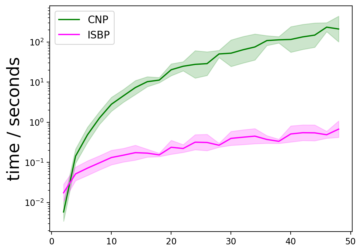
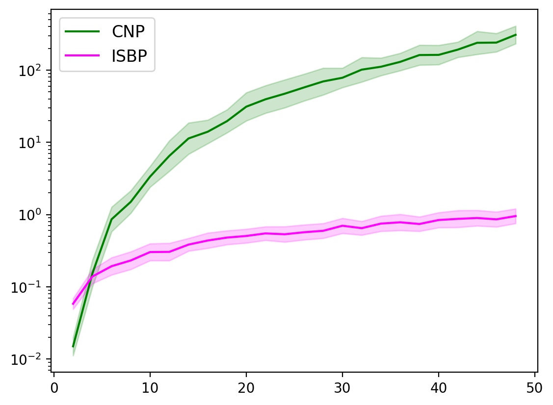
Refer to caption
Refer to caption
Refer to caption
Refer to caption
Refer to caption
Refer to caption
Refer to caption
Refer to caption
Refer to caption
Refer to caption
Refer to caption
Refer to caption
Refer to caption
(a) d=2𝑑2d=2
Refer to caption
(b) d=5𝑑5d=5
Refer to caption
(c) d=10𝑑10d=10
Refer to caption
(d) d=20𝑑20d=20
Figure 8: Performance evaluation of CNP and ISBP. The four rows, from top to bottom, are associated with line graph, HMM, star graph and long star graph respectively. The subplots in the same column share the same value of d𝑑d.

V-B Filtering for collective dynamics

To demonstrate the performance of the methods developed in this paper, we present an example to demonstrate the effectiveness of our MOT framework in filtering problems for collective dynamics. Consider a synthetic particle ensemble with 100001000010000 agents moving over a 20×20202020\times 20 grid, aiming from bottom-left corner to top-right corner. The dynamics of the agents follow a log-linear distribution characterized by four factors: the distance between two positions, the angle between the movements direction and an external force, the angle between the direction of movement and the direction to the goal, and the preference to stay in the original cell. The weights for the log-linear model associated with these four factors are set to be (3,5,5,10)35510(3,5,5,10). This model has been used to model the migration of birds [40, 42].

There are 16 sensors placed over the grid as shown in Figure 9(a). These sensors can not measure the exact locations of the agents. Instead, the measurement of each sensor is a count of agents it currently observes. The probability of an observation decreases exponentially as the distance between the sensor and the agent increases.This type of sensors show up in many real applications. For instance, the sensors can be Wi-Fi hotspots, or cell phone based stations, which can measure the number of phones connected to them. Our goal is to estimate the movement of the whole population using this limited sensor information.

This filtering problem for collective dynamics can be modeled as a MOT problem, or equivalently a constrained marginal inference problem in our framework. In particular, the agents form a HMM and the sensor measurements correspond to constraints on marginal distributions over the observation nodes. The number of discrete states at each node is d=20×20=400𝑑2020400d=20\times 20=400 and the number of nodes depends on the number of time steps. We simulate the model for 15 time steps and run both ISBP and CNP to infer the marginal distributions of the free nodes in order to estimate the group behavior of the 100001000010000 agents. The agents start in two clusters: one in the left-bottom and one in the center-bottom; both aim to reach the right-top corner of the grid in 15 time steps. The results are depicted in Figure 9(b). Both CNP and ISBP give the same estimation result and thus we only display one of them in the figures. As can be seen from the plots, even though the sensor data (center column) is hard to interpret visually, our constrained marginal inference framework can still infer the population movements to a satisfying accuracy.
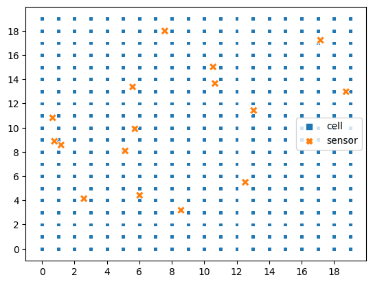
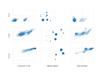
Refer to caption
(a) Sensor locations
Refer to caption
(b) Simulation results
Figure 9: Movement estimation of 10000 agents over a 20×20202020\times 20 grid for 15 time steps: (a) displays the grid and the locations of the sensors; (b) shows the estimation results. The three columns, from left to right, represents the simulated movement of agents at three time steps t=2,9,15𝑡2915t=2,9,15, the sensor measurements, and the estimated agent distributions respectively. The size of the blue dots is proportional to the number of agents.

VI Conclusion

We studied multi-marginal optimal transport problems and pointed out an unexpected connection to probabilistic graphical models. This relation between MOT on graphs and constrained PGMs provides a completely new perspective of both MOT and PGMs, which may have far reaching impact in the future development of both subjects, in both theory and applications. This connection also enables us to adapt the rich class of algorithms in PGMs to tackle difficult MOT problems. In this work, to highlight the key idea of this line of research, we focused on MOT on trees with discrete states. The next step is to generalize the results to more general graphs with cycles as well as continuous state spaces. These are more challenging problems in PGMs, for which exact Bayesian inference is usually too expensive, and one needs to turn to variational inference or sampling based methods [26].

-A Derivation of Constrained Norm-product algorithm (Algorithm 4)

We follow the primal-dual ascent algorithm stated in Lemma 5. Denote 𝝀j={λj,α(𝐱α)}subscript𝝀𝑗subscript𝜆𝑗𝛼subscript𝐱𝛼\boldsymbol{\lambda}_{j}=\left\{\lambda_{j,\alpha}({\mathbf{x}}_{\alpha})\right\} and 𝝂j={νj,α(𝐱α)}subscript𝝂𝑗subscript𝜈𝑗𝛼subscript𝐱𝛼\boldsymbol{\nu}_{j}=\left\{\nu_{j,\alpha}({\mathbf{x}}_{\alpha})\right\}. For the sake of convenience, we introduce the following notation

ψ^j,α(𝐱α)subscript^𝜓𝑗𝛼subscript𝐱𝛼\displaystyle\hat{\psi}_{j,\alpha}({\mathbf{x}}_{\alpha}) :=ψα(𝐱α)exp(νj,α(𝐱α)),assignabsentsubscript𝜓𝛼subscript𝐱𝛼subscript𝜈𝑗𝛼subscript𝐱𝛼\displaystyle:=\psi_{\alpha}({\mathbf{x}}_{\alpha})\exp(-\nu_{j,\alpha}({\mathbf{x}}_{\alpha})), (62)
c^jαsubscript^𝑐𝑗𝛼\displaystyle\hat{c}_{j\alpha} :=cα+cjα,assignabsentsubscript𝑐𝛼subscript𝑐𝑗𝛼\displaystyle:=c_{\alpha}+c_{j\alpha},
c^jsubscript^𝑐𝑗\displaystyle\hat{c}_{j} :=cj+αN(j)cα.assignabsentsubscript𝑐𝑗subscript𝛼𝑁𝑗subscript𝑐𝛼\displaystyle:=c_{j}+\sum_{\alpha\in N(j)}c_{\alpha}.

For a fixed 1jJ1𝑗𝐽1\leq j\leq J, the step (54b) in the primal-dual ascent algorithm requires solving

min𝐛dom(f)dom(hj)f(𝐛)+hj(𝐛)+𝐛T𝝂j.subscript𝐛𝑑𝑜𝑚𝑓𝑑𝑜𝑚subscript𝑗𝑓𝐛subscript𝑗𝐛superscript𝐛𝑇subscript𝝂𝑗\min_{{\mathbf{b}}\in dom(f)\cap dom(h_{j})}f({\mathbf{b}})+h_{j}({\mathbf{b}})+{\mathbf{b}}^{T}\boldsymbol{\nu}_{j}.

Recall that f(𝐛)=f^(𝐛)+δ𝒫(𝐛)𝑓𝐛^𝑓𝐛subscript𝛿𝒫𝐛f({\mathbf{b}})=\hat{f}({\mathbf{b}})+\delta_{\mathcal{P}}({\mathbf{b}}), hj(𝐛)=h^j(𝐛)+δ(𝐛)subscript𝑗𝐛subscript^𝑗𝐛subscript𝛿𝐛h_{j}({\mathbf{b}})=\hat{h}_{j}({\mathbf{b}})+\delta_{\mathcal{M}}({\mathbf{b}}) where

\displaystyle{\mathcal{M}} =\displaystyle= {𝐛:𝐱α\xjbα(𝐱α)=bj(xj),jV,αN(j),bj(xj)=μj(xj),jΓ},conditional-set𝐛formulae-sequencesubscript\subscript𝐱𝛼subscript𝑥𝑗subscript𝑏𝛼subscript𝐱𝛼subscript𝑏𝑗subscript𝑥𝑗formulae-sequencefor-all𝑗𝑉formulae-sequence𝛼𝑁𝑗formulae-sequencesubscript𝑏𝑗subscript𝑥𝑗subscript𝜇𝑗subscript𝑥𝑗for-all𝑗Γ\displaystyle\Big{\{}{\mathbf{b}}:\sum_{{\bf x}_{\alpha}\backslash x_{j}}b_{\alpha}({\bf x}_{\alpha})=b_{j}(x_{j}),\forall j\in V,\alpha\in N(j),\,b_{j}(x_{j})=\mu_{j}(x_{j}),\,\forall j\in\Gamma\Big{\}},
𝒫𝒫\displaystyle{\mathcal{P}} =\displaystyle= {𝐛:𝐱αbα(𝐱α)=1,αF},conditional-set𝐛formulae-sequencesubscriptsubscript𝐱𝛼subscript𝑏𝛼subscript𝐱𝛼1for-all𝛼𝐹\displaystyle\Big{\{}{\mathbf{b}}:\sum_{{\bf x}_{\alpha}}b_{\alpha}({\bf x}_{\alpha})=1,\quad\forall\alpha\in F\Big{\}},
f^(𝐛)^𝑓𝐛\displaystyle\hat{f}({\mathbf{b}}) =\displaystyle= 𝐱α,αFbα(𝐱α)lnψα(𝐱α)αFϵcα(𝐛α),subscriptsubscript𝐱𝛼𝛼𝐹subscript𝑏𝛼subscript𝐱𝛼subscript𝜓𝛼subscript𝐱𝛼subscript𝛼𝐹italic-ϵsubscript𝑐𝛼subscript𝐛𝛼\displaystyle-\sum_{{\mathbf{x}}_{\alpha},\alpha\in F}b_{\alpha}({\mathbf{x}}_{\alpha})\ln\psi_{\alpha}({\mathbf{x}}_{\alpha})-\sum_{\alpha\in F}\epsilon\,c_{\alpha}{\mathcal{H}}({\mathbf{b}}_{\alpha}),
h^j(𝐛)subscript^𝑗𝐛\displaystyle\hat{h}_{j}({\mathbf{b}}) =\displaystyle= xjbj(xj)lnϕj(xj)ϵcj(𝐛j)αN(j)ϵcjα((𝐛α)(𝐛j)).subscriptsubscript𝑥𝑗subscript𝑏𝑗subscript𝑥𝑗subscriptitalic-ϕ𝑗subscript𝑥𝑗italic-ϵsubscript𝑐𝑗subscript𝐛𝑗subscript𝛼𝑁𝑗italic-ϵsubscript𝑐𝑗𝛼subscript𝐛𝛼subscript𝐛𝑗\displaystyle-\sum_{x_{j}}b_{j}(x_{j})\ln\phi_{j}(x_{j})-\epsilon\,c_{j}{\mathcal{H}}({\mathbf{b}}_{j})-\sum_{\alpha\in N(j)}\epsilon\,c_{j\alpha}({\mathcal{H}}({\mathbf{b}}_{\alpha})-{\mathcal{H}}({\mathbf{b}}_{j})).

Thus, for any fixed 1jJ1𝑗𝐽1\leq j\leq J, step (54b) of the primal-dual ascent algorithm can be reformulated as

min𝐛j,𝐛α,αN(j)subscriptsubscript𝐛𝑗subscript𝐛𝛼𝛼𝑁𝑗\displaystyle\min_{{\mathbf{b}}_{j},{\mathbf{b}}_{\alpha},\alpha\in N(j)}\!\!\!\! {xjbj(xj)lnϕj(xj)αN(j)𝐱αbα(𝐱α)lnψ^j,α(𝐱α)ϵc^j(𝐛j)αN(j)ϵc^jα((𝐛α)(𝐛j))}subscriptsubscript𝑥𝑗subscript𝑏𝑗subscript𝑥𝑗subscriptitalic-ϕ𝑗subscript𝑥𝑗subscript𝛼𝑁𝑗subscriptsubscript𝐱𝛼subscript𝑏𝛼subscript𝐱𝛼subscript^𝜓𝑗𝛼subscript𝐱𝛼italic-ϵsubscript^𝑐𝑗subscript𝐛𝑗subscript𝛼𝑁𝑗italic-ϵsubscript^𝑐𝑗𝛼subscript𝐛𝛼subscript𝐛𝑗\displaystyle\!\!\!\!\Bigg{\{}\!-\!\sum_{x_{j}}b_{j}(x_{j})\ln\phi_{j}(x_{j})\!-\!\sum_{\alpha\in N(j)}\sum_{{\mathbf{x}}_{\alpha}}b_{\alpha}({\mathbf{x}}_{\alpha})\ln\hat{\psi}_{j,\alpha}({\mathbf{x}}_{\alpha})\!-\!\epsilon\hat{c}_{j}{\mathcal{H}}({\mathbf{b}}_{j})\!-\!\sum_{\alpha\in N(j)}\epsilon\hat{c}_{j\alpha}({\mathcal{H}}({\mathbf{b}}_{\alpha})-{\mathcal{H}}({\mathbf{b}}_{j}))\Bigg{\}} (63a)
subject to 𝐱αbα(𝐱α)=1,𝐱α\xjbα(𝐱α)=bj(xj),xj,αN(j),formulae-sequencesubscriptsubscript𝐱𝛼subscript𝑏𝛼subscript𝐱𝛼1formulae-sequencesubscript\subscript𝐱𝛼subscript𝑥𝑗subscript𝑏𝛼subscript𝐱𝛼subscript𝑏𝑗subscript𝑥𝑗for-allsubscript𝑥𝑗𝛼𝑁𝑗\displaystyle\!\!\!\!\sum_{{\mathbf{x}}_{\alpha}}b_{\alpha}({\mathbf{x}}_{\alpha})=1,\quad\sum_{{\mathbf{x}}_{\alpha}\backslash x_{j}}b_{\alpha}({\mathbf{x}}_{\alpha})=b_{j}(x_{j}),\quad\forall x_{j},\alpha\in N(j), (63c)
bj(xj)=μj(xj),xj,ifjΓ.formulae-sequencesubscript𝑏𝑗subscript𝑥𝑗subscript𝜇𝑗subscript𝑥𝑗for-allsubscript𝑥𝑗if𝑗Γ\displaystyle\!\!\!\!b_{j}(x_{j})=\mu_{j}(x_{j}),\quad\forall x_{j},~{}\mbox{if}~{}j\in\Gamma.

Note that when jΓ𝑗Γj\in\Gamma, the above problem has an extra constraint (63c) compared to the cases where jΓ𝑗Γj\notin\Gamma.

We next derive a closed form solution 𝐛j,𝐛αsuperscriptsubscript𝐛𝑗superscriptsubscript𝐛𝛼{\mathbf{b}}_{j}^{*},{\mathbf{b}}_{\alpha}^{*} to (63). The constraint (63c) implies that 𝐛jsubscript𝐛𝑗{\mathbf{b}}_{j} is a marginal distribution of 𝐛αsubscript𝐛𝛼{\mathbf{b}}_{\alpha}, thus, 𝐛αsubscript𝐛𝛼{\mathbf{b}}_{\alpha} can be rewritten in terms of conditional distribution 𝐛αjsubscript𝐛conditional𝛼𝑗{\mathbf{b}}_{\alpha\mid j} as

bα(𝐱α)=bj(xj)bαj(𝐱αxj).subscript𝑏𝛼subscript𝐱𝛼subscript𝑏𝑗subscript𝑥𝑗subscript𝑏conditional𝛼𝑗conditionalsubscript𝐱𝛼subscript𝑥𝑗b_{\alpha}({\mathbf{x}}_{\alpha})=b_{j}(x_{j})b_{\alpha\mid j}({\mathbf{x}}_{\alpha}\mid x_{j}). (64)

The entropy (𝐛α)subscript𝐛𝛼{\mathcal{H}}({\mathbf{b}}_{\alpha}) can be rewritten as [59]

(𝐛α)=(𝐛j)+xjbj(xj)(𝐛α|j)subscript𝐛𝛼subscript𝐛𝑗subscriptsubscript𝑥𝑗subscript𝑏𝑗subscript𝑥𝑗subscript𝐛conditional𝛼𝑗{\mathcal{H}}({\mathbf{b}}_{\alpha})={\mathcal{H}}({\mathbf{b}}_{j})+\sum_{x_{j}}b_{j}(x_{j}){\mathcal{H}}({\mathbf{b}}_{\alpha|j})

where

(𝐛α|j)=𝐱α\xjbαj(𝐱αxj)lnbαj(𝐱αxj).subscript𝐛conditional𝛼𝑗subscript\subscript𝐱𝛼subscript𝑥𝑗subscript𝑏conditional𝛼𝑗conditionalsubscript𝐱𝛼subscript𝑥𝑗subscript𝑏conditional𝛼𝑗conditionalsubscript𝐱𝛼subscript𝑥𝑗{\mathcal{H}}({\mathbf{b}}_{\alpha|j})=-\sum_{{\mathbf{x}}_{\alpha}\backslash x_{j}}b_{\alpha\mid j}({\mathbf{x}}_{\alpha}\mid x_{j})\ln b_{\alpha\mid j}({\mathbf{x}}_{\alpha}\mid x_{j}).

Thus, in terms of new variables 𝐛j,𝐛αj,αN(j)subscript𝐛𝑗subscript𝐛conditional𝛼𝑗𝛼𝑁𝑗{\mathbf{b}}_{j},{\mathbf{b}}_{\alpha\mid j},\alpha\in N(j), the optimization problem (63) reads

min𝐛j{xjbj(xj)lnϕj(xj)ϵc^j(𝐛j)+xjbj(xj)αN(j)ϵc^jα[min𝐛αj𝐱αxjbαj(𝐱αxj)lnψ^j,α1/(ϵc^jα)(𝐱α)(𝐛αj)]}subscriptsubscript𝐛𝑗subscriptsubscript𝑥𝑗subscript𝑏𝑗subscript𝑥𝑗subscriptitalic-ϕ𝑗subscript𝑥𝑗italic-ϵsubscript^𝑐𝑗subscript𝐛𝑗subscriptsubscript𝑥𝑗subscript𝑏𝑗subscript𝑥𝑗subscript𝛼𝑁𝑗italic-ϵsubscript^𝑐𝑗𝛼delimited-[]subscriptsubscriptsubscript𝐛conditional𝛼𝑗subscriptsubscript𝐱𝛼subscript𝑥𝑗subscript𝑏conditional𝛼𝑗conditionalsubscript𝐱𝛼subscript𝑥𝑗superscriptsubscript^𝜓𝑗𝛼1italic-ϵsubscript^𝑐𝑗𝛼subscript𝐱𝛼subscript𝐛conditional𝛼𝑗\min_{{\mathbf{b}}_{j}}\Bigg{\{}-\sum_{x_{j}}b_{j}(x_{j})\ln\phi_{j}(x_{j})-\epsilon\hat{c}_{j}{\mathcal{H}}({\mathbf{b}}_{j})+\sum_{x_{j}}b_{j}(x_{j})\sum_{\alpha\in N(j)}\epsilon\hat{c}_{j\alpha}\bigg{[}\underbrace{\min_{{\mathbf{b}}_{\alpha\mid j}}-\sum_{{\mathbf{x}}_{\alpha}\setminus x_{j}}b_{\alpha\mid j}({\mathbf{x}}_{\alpha}\mid x_{j})\ln\hat{\psi}_{j,\alpha}^{1/(\epsilon\hat{c}_{j\alpha})}({\mathbf{x}}_{\alpha})-{\mathcal{H}}({\mathbf{b}}_{\alpha\mid j})}_{\star}\bigg{]}\Bigg{\}} (65)

together with the extra constraint 𝐛j=𝝁jsubscript𝐛𝑗subscript𝝁𝑗{\mathbf{b}}_{j}=\boldsymbol{\mu}_{j} if jΓ𝑗Γj\in\Gamma. One advantage of this reformulation is that the problem now can be optimized over 𝐛αjsubscript𝐛conditional𝛼𝑗{\mathbf{b}}_{\alpha\mid j} first and then over 𝐛jsubscript𝐛𝑗{\mathbf{b}}_{j}.

Minimizing (65) over 𝐛αjsubscript𝐛conditional𝛼𝑗{\mathbf{b}}_{\alpha\mid j} is a standard exercise, and the minimizer is

bαj(𝐱αxj)=ψ^j,α(𝐱α)1/ϵc^jα/𝐱αxjψ^j,α(𝐱α)1/ϵc^jα.superscriptsubscript𝑏conditional𝛼𝑗conditionalsubscript𝐱𝛼subscript𝑥𝑗subscript^𝜓𝑗𝛼superscriptsubscript𝐱𝛼1italic-ϵsubscript^𝑐𝑗𝛼subscriptsubscript𝐱𝛼subscript𝑥𝑗subscript^𝜓𝑗𝛼superscriptsubscript𝐱𝛼1italic-ϵsubscript^𝑐𝑗𝛼b_{\alpha\mid j}^{*}({\mathbf{x}}_{\alpha}\mid x_{j})=\hat{\psi}_{j,\alpha}({\mathbf{x}}_{\alpha})^{1/\epsilon\hat{c}_{j\alpha}}/\sum_{{\mathbf{x}}_{\alpha}\setminus x_{j}}\hat{\psi}_{j,\alpha}({\mathbf{x}}_{\alpha})^{1/\epsilon\hat{c}_{j\alpha}}.

Thus, the value for block ()(\star) is

()=ln𝐱αxjψ^j,α(𝐱α)1/ϵc^jα.subscriptsubscript𝐱𝛼subscript𝑥𝑗subscript^𝜓𝑗𝛼superscriptsubscript𝐱𝛼1italic-ϵsubscript^𝑐𝑗𝛼\displaystyle(\star)=-\ln{\sum_{{\mathbf{x}}_{\alpha}\setminus x_{j}}\hat{\psi}_{j,\alpha}({\mathbf{x}}_{\alpha})^{1/\epsilon\hat{c}_{j\alpha}}}.

Denote

mαj(xj)=(𝐱αxjψ^j,α(𝐱α)1/ϵc^jα)ϵc^jα,subscript𝑚𝛼𝑗subscript𝑥𝑗superscriptsubscriptsubscript𝐱𝛼subscript𝑥𝑗subscript^𝜓𝑗𝛼superscriptsubscript𝐱𝛼1italic-ϵsubscript^𝑐𝑗𝛼italic-ϵsubscript^𝑐𝑗𝛼m_{\alpha\rightarrow j}(x_{j})=\left(\sum_{{\mathbf{x}}_{\alpha}\setminus x_{j}}\hat{\psi}_{j,\alpha}({\mathbf{x}}_{\alpha})^{1/\epsilon\hat{c}_{j\alpha}}\right)^{\epsilon\hat{c}_{j\alpha}}, (66)

then (65) with optimal 𝐛αjsubscript𝐛conditional𝛼𝑗{\mathbf{b}}_{\alpha\mid j} can be simplified as

min𝐛j[(𝐛j)xjbj(xj)lnϕj1/ϵc^j(xj)αN(j)mαj1/ϵc^j(xj)].subscriptsubscript𝐛𝑗subscript𝐛𝑗subscriptsubscript𝑥𝑗subscript𝑏𝑗subscript𝑥𝑗superscriptsubscriptitalic-ϕ𝑗1italic-ϵsubscript^𝑐𝑗subscript𝑥𝑗subscriptproduct𝛼𝑁𝑗superscriptsubscript𝑚𝛼𝑗1italic-ϵsubscript^𝑐𝑗subscript𝑥𝑗\min_{{\mathbf{b}}_{j}}\left[-{\mathcal{H}}({\mathbf{b}}_{j})-\sum_{x_{j}}b_{j}(x_{j})\ln\phi_{j}^{1/\epsilon\hat{c}_{j}}(x_{j})\prod_{\alpha\in N(j)}m_{\alpha\rightarrow j}^{1/\epsilon\hat{c}_{j}}(x_{j})\right]. (67)

When jΓ𝑗Γj\in\Gamma, 𝐛j=𝝁jsubscript𝐛𝑗subscript𝝁𝑗{\mathbf{b}}_{j}=\boldsymbol{\mu}_{j} is the only feasible point; 𝐛j=𝝁jsuperscriptsubscript𝐛𝑗subscript𝝁𝑗{\mathbf{b}}_{j}^{*}=\boldsymbol{\mu}_{j}. When jΓ𝑗Γj\notin\Gamma, (67) is again a standard exercise with the unique minimizer being

bj(xj)(ϕj(xj)αN(j)mαj(xj))1/ϵc^j.proportional-tosuperscriptsubscript𝑏𝑗subscript𝑥𝑗superscriptsubscriptitalic-ϕ𝑗subscript𝑥𝑗subscriptproduct𝛼𝑁𝑗subscript𝑚𝛼𝑗subscript𝑥𝑗1italic-ϵsubscript^𝑐𝑗b_{j}^{*}(x_{j})\propto\left(\phi_{j}(x_{j})\prod_{\alpha\in N(j)}m_{\alpha\rightarrow j}(x_{j})\right)^{1/\epsilon\hat{c}_{j}}. (68)

Combining 𝐛jsuperscriptsubscript𝐛𝑗{\mathbf{b}}_{j}^{*} and 𝐛α|jsuperscriptsubscript𝐛conditional𝛼𝑗{\mathbf{b}}_{\alpha|j}^{*}, we obtain

bα(𝐱α)=bj(xj)bα|j(𝐱α|xj)=bj(xj)mαj1/ϵc^jα(xj)ψ^j,α(𝐱α)1/ϵc^jα.superscriptsubscript𝑏𝛼subscript𝐱𝛼superscriptsubscript𝑏𝑗subscript𝑥𝑗superscriptsubscript𝑏conditional𝛼𝑗conditionalsubscript𝐱𝛼subscript𝑥𝑗superscriptsubscript𝑏𝑗subscript𝑥𝑗superscriptsubscript𝑚𝛼𝑗1italic-ϵsubscript^𝑐𝑗𝛼subscript𝑥𝑗subscript^𝜓𝑗𝛼superscriptsubscript𝐱𝛼1italic-ϵsubscript^𝑐𝑗𝛼b_{\alpha}^{*}({\mathbf{x}}_{\alpha})=b_{j}^{*}(x_{j})b_{\alpha|j}^{*}({\mathbf{x}}_{\alpha}|x_{j})=\frac{b_{j}^{*}(x_{j})}{m_{\alpha\rightarrow j}^{1/\epsilon\hat{c}_{j\alpha}}(x_{j})}\hat{\psi}_{j,\alpha}({\mathbf{x}}_{\alpha})^{1/\epsilon\hat{c}_{j\alpha}}. (69)

Next, we move to step (54c) of the primal-dual ascent algorithm (Lemma 5), which reads

𝝀j𝝂jf^(𝐛)+AT𝝈subscript𝝀𝑗subscript𝝂𝑗^𝑓superscript𝐛superscript𝐴𝑇𝝈\boldsymbol{\lambda}_{j}\leftarrow-\boldsymbol{\nu}_{j}-\nabla\hat{f}({\mathbf{b}}^{*})+A^{T}\boldsymbol{\sigma}

with 𝝈𝝈\boldsymbol{\sigma} being an arbitrary vector. The vector AT𝝈superscript𝐴𝑇𝝈A^{T}\boldsymbol{\sigma} spans the orthogonal space to the domain {\mathcal{B}} (see Lemma 5) of f𝑓f. In our problem, =𝒫𝒫{\mathcal{B}}={\mathcal{P}} is the probability simplex, thus AT𝝈superscript𝐴𝑇𝝈A^{T}\boldsymbol{\sigma} is in alignment with 𝟏1{\bf 1}, the vector with all 1 entries. It follows that

λj,α(𝐱α)=νj,α(𝐱α)f^(bα(𝐱α))+σα𝟏.subscript𝜆𝑗𝛼subscript𝐱𝛼subscript𝜈𝑗𝛼subscript𝐱𝛼^𝑓superscriptsubscript𝑏𝛼subscript𝐱𝛼subscript𝜎𝛼1\lambda_{j,\alpha}({\mathbf{x}}_{\alpha})=-\nu_{j,\alpha}({\mathbf{x}}_{\alpha})-\nabla\hat{f}(b_{\alpha}^{*}({\mathbf{x}}_{\alpha}))+\sigma_{\alpha}{\bf 1}. (70)

The value of f^(bα(𝐱α))^𝑓superscriptsubscript𝑏𝛼subscript𝐱𝛼\nabla\hat{f}(b_{\alpha}^{*}({\mathbf{x}}_{\alpha})) is

f^(bα(𝐱α))=lnψα(𝐱α)+ϵcα(lnbα(𝐱α)+1).^𝑓superscriptsubscript𝑏𝛼subscript𝐱𝛼subscript𝜓𝛼subscript𝐱𝛼italic-ϵsubscript𝑐𝛼superscriptsubscript𝑏𝛼subscript𝐱𝛼1\nabla\hat{f}(b_{\alpha}^{*}({\mathbf{x}}_{\alpha}))=-\ln{\psi_{\alpha}({\mathbf{x}}_{\alpha})}+\epsilon c_{\alpha}\left(\ln{b_{\alpha}^{*}({\mathbf{x}}_{\alpha})+1}\right).

Define njα(𝐱α)subscript𝑛𝑗𝛼subscript𝐱𝛼n_{j\rightarrow\alpha}({\mathbf{x}}_{\alpha}) as

njα(𝐱α):=exp(λj,α(𝐱α)),assignsubscript𝑛𝑗𝛼subscript𝐱𝛼subscript𝜆𝑗𝛼subscript𝐱𝛼n_{j\rightarrow\alpha}({\mathbf{x}}_{\alpha}):=\exp(-\lambda_{j,\alpha}({\mathbf{x}}_{\alpha})), (71)

then, in view of (69),

njα(𝐱α)subscript𝑛𝑗𝛼subscript𝐱𝛼\displaystyle n_{j\rightarrow\alpha}({\mathbf{x}}_{\alpha}) exp(νj,α(𝐱α)lnψα(𝐱α))(bα(𝐱α))ϵcαproportional-toabsentsubscript𝜈𝑗𝛼subscript𝐱𝛼subscript𝜓𝛼subscript𝐱𝛼superscriptsuperscriptsubscript𝑏𝛼subscript𝐱𝛼italic-ϵsubscript𝑐𝛼\displaystyle\propto\exp(\nu_{j,\alpha}({\mathbf{x}}_{\alpha})-\ln\psi_{\alpha}({\mathbf{x}}_{\alpha}))(b_{\alpha}^{*}({\mathbf{x}}_{\alpha}))^{\epsilon c_{\alpha}}
=ψ^j,α1(𝐱α)(bj(xj)mαj1/ϵc^jα(xj))ϵcαψ^j,αcα/c^jα(𝐱α)absentsuperscriptsubscript^𝜓𝑗𝛼1subscript𝐱𝛼superscriptsuperscriptsubscript𝑏𝑗subscript𝑥𝑗superscriptsubscript𝑚𝛼𝑗1italic-ϵsubscript^𝑐𝑗𝛼subscript𝑥𝑗italic-ϵsubscript𝑐𝛼superscriptsubscript^𝜓𝑗𝛼subscript𝑐𝛼subscript^𝑐𝑗𝛼subscript𝐱𝛼\displaystyle=\hat{\psi}_{j,\alpha}^{-1}({\mathbf{x}}_{\alpha})\left(\frac{b_{j}^{*}(x_{j})}{m_{\alpha\rightarrow j}^{1/\epsilon\hat{c}_{j\alpha}}(x_{j})}\right)^{\epsilon c_{\alpha}}\hat{\psi}_{j,\alpha}^{c_{\alpha}/\hat{c}_{j\alpha}}({\mathbf{x}}_{\alpha})
=(bj(xj)mαj1/ϵc^jα(xj))ϵcαψ^j,αcα/c^jα1(𝐱α)absentsuperscriptsuperscriptsubscript𝑏𝑗subscript𝑥𝑗superscriptsubscript𝑚𝛼𝑗1italic-ϵsubscript^𝑐𝑗𝛼subscript𝑥𝑗italic-ϵsubscript𝑐𝛼superscriptsubscript^𝜓𝑗𝛼subscript𝑐𝛼subscript^𝑐𝑗𝛼1subscript𝐱𝛼\displaystyle=\left(\frac{b_{j}^{*}(x_{j})}{m_{\alpha\rightarrow j}^{1/\epsilon\hat{c}_{j\alpha}}(x_{j})}\right)^{\epsilon c_{\alpha}}\hat{\psi}_{j,\alpha}^{c_{\alpha}/\hat{c}_{j\alpha}-1}({\mathbf{x}}_{\alpha})
=(bj(xj)mαj1/ϵc^jα(xj))ϵcαψ^j,αcjα/c^jα(𝐱α),absentsuperscriptsuperscriptsubscript𝑏𝑗subscript𝑥𝑗superscriptsubscript𝑚𝛼𝑗1italic-ϵsubscript^𝑐𝑗𝛼subscript𝑥𝑗italic-ϵsubscript𝑐𝛼superscriptsubscript^𝜓𝑗𝛼subscript𝑐𝑗𝛼subscript^𝑐𝑗𝛼subscript𝐱𝛼\displaystyle=\left(\frac{b_{j}^{*}(x_{j})}{m_{\alpha\rightarrow j}^{1/\epsilon\hat{c}_{j\alpha}}(x_{j})}\right)^{\epsilon c_{\alpha}}\hat{\psi}_{j,\alpha}^{-c_{j\alpha}/\hat{c}_{j\alpha}}({\mathbf{x}}_{\alpha}), (72)

where the last equation is due to c^jα=cα+cjαsubscript^𝑐𝑗𝛼subscript𝑐𝛼subscript𝑐𝑗𝛼\hat{c}_{j\alpha}=c_{\alpha}+c_{j\alpha}. By step (54a) of the primal-dual ascent algorithm, νj,α=iN(α)jλi,α(𝐱α)subscript𝜈𝑗𝛼subscript𝑖𝑁𝛼𝑗subscript𝜆𝑖𝛼subscript𝐱𝛼\nu_{j,\alpha}=\sum_{i\in N(\alpha)\setminus j}\lambda_{i,\alpha}({\mathbf{x}}_{\alpha}). Combining it with (62) and (71) yields

ψ^j,α(𝐱α)subscript^𝜓𝑗𝛼subscript𝐱𝛼\displaystyle\hat{\psi}_{j,\alpha}({\mathbf{x}}_{\alpha}) =\displaystyle= ψα(𝐱α)iN(α)jexp(λi,α(𝐱α))subscript𝜓𝛼subscript𝐱𝛼subscriptproduct𝑖𝑁𝛼𝑗subscript𝜆𝑖𝛼subscript𝐱𝛼\displaystyle\psi_{\alpha}({\mathbf{x}}_{\alpha})\prod_{i\in N(\alpha)\setminus j}\exp(-\lambda_{i,\alpha}({\mathbf{x}}_{\alpha})) (73)
=\displaystyle= ψα(𝐱α)iN(α)jniα(𝐱α).subscript𝜓𝛼subscript𝐱𝛼subscriptproduct𝑖𝑁𝛼𝑗subscript𝑛𝑖𝛼subscript𝐱𝛼\displaystyle\psi_{\alpha}({\mathbf{x}}_{\alpha})\prod_{i\in N(\alpha)\setminus j}n_{i\rightarrow\alpha}({\mathbf{x}}_{\alpha}).

Finally, plugging (73) into (66) leads to

mαj(xj)=(𝐱αxj(ψα(𝐱α)iN(α)jniα(𝐱α))1/ϵc^jα)ϵc^jα.subscript𝑚𝛼𝑗subscript𝑥𝑗superscriptsubscriptsubscript𝐱𝛼subscript𝑥𝑗superscriptsubscript𝜓𝛼subscript𝐱𝛼subscriptproduct𝑖𝑁𝛼𝑗subscript𝑛𝑖𝛼subscript𝐱𝛼1italic-ϵsubscript^𝑐𝑗𝛼italic-ϵsubscript^𝑐𝑗𝛼m_{\alpha\rightarrow j}(x_{j})=\left(\sum_{{\mathbf{x}}_{\alpha}\setminus x_{j}}\left(\psi_{\alpha}({\mathbf{x}}_{\alpha})\prod_{i\in N(\alpha)\setminus j}n_{i\rightarrow\alpha}({\mathbf{x}}_{\alpha})\right)^{1/\epsilon\hat{c}_{j\alpha}}\right)^{\epsilon\hat{c}_{j\alpha}}.

Plugging (73) into (72), in view of the different forms of 𝐛jsuperscriptsubscript𝐛𝑗{\mathbf{b}}_{j}^{*} for jΓ𝑗Γj\in\Gamma and jΓ𝑗Γj\notin\Gamma, we obtain

njα(𝐱α)(ϕj1/c^j(xj)βN(j)mβj1/c^j(xj)mαj1/c^jα(xj))cα(ψα(𝐱α)iN(α)jniα(𝐱α))cjα/c^jαproportional-tosubscript𝑛𝑗𝛼subscript𝐱𝛼superscriptsuperscriptsubscriptitalic-ϕ𝑗1subscript^𝑐𝑗subscript𝑥𝑗subscriptproduct𝛽𝑁𝑗superscriptsubscript𝑚𝛽𝑗1subscript^𝑐𝑗subscript𝑥𝑗superscriptsubscript𝑚𝛼𝑗1subscript^𝑐𝑗𝛼subscript𝑥𝑗subscript𝑐𝛼superscriptsubscript𝜓𝛼subscript𝐱𝛼subscriptproduct𝑖𝑁𝛼𝑗subscript𝑛𝑖𝛼subscript𝐱𝛼subscript𝑐𝑗𝛼subscript^𝑐𝑗𝛼n_{j\rightarrow\alpha}({\mathbf{x}}_{\alpha})\propto\left(\frac{\phi_{j}^{1/\hat{c}_{j}}(x_{j})\prod_{\beta\in N(j)}m_{\beta\rightarrow j}^{1/\hat{c}_{j}}(x_{j})}{m_{\alpha\rightarrow j}^{1/\hat{c}_{j\alpha}}(x_{j})}\right)^{c_{\alpha}}\left(\psi_{\alpha}({\mathbf{x}}_{\alpha})\prod_{i\in N(\alpha)\setminus j}n_{i\rightarrow\alpha}({\mathbf{x}}_{\alpha})\right)^{-c_{j\alpha}/\hat{c}_{j\alpha}}

for jΓ𝑗Γj\notin\Gamma, and

njα(𝐱α)(μj(xj)mαj1/ϵc^jα(𝐱α))ϵcα(ψα(𝐱α)iN(α)jniα(𝐱α))cjα/c^jαproportional-tosubscript𝑛𝑗𝛼subscript𝐱𝛼superscriptsubscript𝜇𝑗subscript𝑥𝑗superscriptsubscript𝑚𝛼𝑗1italic-ϵsubscript^𝑐𝑗𝛼subscript𝐱𝛼italic-ϵsubscript𝑐𝛼superscriptsubscript𝜓𝛼subscript𝐱𝛼subscriptproduct𝑖𝑁𝛼𝑗subscript𝑛𝑖𝛼subscript𝐱𝛼subscript𝑐𝑗𝛼subscript^𝑐𝑗𝛼n_{j\rightarrow\alpha}({\mathbf{x}}_{\alpha})\propto\left(\frac{\mu_{j}(x_{j})}{m_{\alpha\rightarrow j}^{1/\epsilon\hat{c}_{j\alpha}}({\mathbf{x}}_{\alpha})}\right)^{\epsilon c_{\alpha}}\left(\psi_{\alpha}({\mathbf{x}}_{\alpha})\prod_{i\in N(\alpha)\setminus j}n_{i\rightarrow\alpha}({\mathbf{x}}_{\alpha})\right)^{-c_{j\alpha}/\hat{c}_{j\alpha}}

for jΓ𝑗Γj\in\Gamma. This concludes the derivation.

References

  • [1] L. C. Evans and W. Gangbo, Differential equations methods for the Monge-Kantorovich mass transfer problem.   American Mathematical Soc., 1999, vol. 653.
  • [2] C. Villani, Topics in optimal transportation.   American Mathematical Soc., 2003, no. 58.
  • [3] S. Haker, L. Zhu, A. Tannenbaum, and S. Angenent, “Optimal mass transport for registration and warping,” International Journal of Computer Vision, vol. 60, no. 3, pp. 225–240, 2004.
  • [4] M. Mueller, P. Karasev, I. Kolesov, and A. Tannenbaum, “Optical flow estimation for flame detection in videos,” IEEE Transactions on image processing, vol. 22, no. 7, pp. 2786–2797, 2013.
  • [5] Y. Chen, T. T. Georgiou, and M. Pavon, “On the relation between optimal transport and Schrödinger bridges: A stochastic control viewpoint,” Journal of Optimization Theory and Applications, vol. 169, no. 2, pp. 671–691, 2016.
  • [6] Y. Chen, T. T. Georgiou, and M. Pavon, “Optimal transport over a linear dynamical system,” IEEE Transactions on Automatic Control, vol. 62, no. 5, pp. 2137–2152, 2017.
  • [7] A. Galichon, Optimal Transport Methods in Economics.   Princeton University Press, 2016.
  • [8] Y. Chen, “Modeling and control of collective dynamics: From Schrödinger bridges to optimal mass transport,” Ph.D. dissertation, University of Minnesota, 2016.
  • [9] M. Arjovsky, S. Chintala, and L. Bottou, “Wasserstein generative adversarial networks,” in International conference on machine learning, 2017, pp. 214–223.
  • [10] M. Cuturi, “Sinkhorn distances: Lightspeed computation of optimal transport,” in Advances in neural information processing systems, 2013, pp. 2292–2300.
  • [11] W. E. Deming and F. F. Stephan, “On a least squares adjustment of a sampled frequency table when the expected marginal totals are known,” The Annals of Mathematical Statistics, vol. 11, no. 4, pp. 427–444, 1940.
  • [12] W. Gangbo and A. Świech, “Optimal maps for the multidimensional Monge-Kantorovich problem,” Communications on Pure and Applied Mathematics: A Journal Issued by the Courant Institute of Mathematical Sciences, vol. 51, no. 1, pp. 23–45, 1998.
  • [13] G. Carlier, “On a class of multidimensional optimal transportation problems,” Journal of convex analysis, vol. 10, no. 2, pp. 517–530, 2003.
  • [14] B. Pass, “On the local structure of optimal measures in the multi-marginal optimal transportation problem,” Calculus of Variations and Partial Differential Equations, vol. 43, no. 3-4, pp. 529–536, 2012.
  • [15] B. Pass, “Multi-marginal optimal transport: theory and applications,” ESAIM: Mathematical Modelling and Numerical Analysis, vol. 49, no. 6, pp. 1771–1790, 2015.
  • [16] L. Nenna, “Numerical methods for multi-marginal optimal transportation,” Ph.D. dissertation, 2016.
  • [17] F. Elvander, I. Haasler, A. Jakobsson, and J. Karlsson, “Multi-marginal optimal transport using partial information with applications in robust localization and sensor fusion,” Signal Processing, p. 107474, 2020.
  • [18] J.-D. Benamou, G. Carlier, and L. Nenna, “Generalized incompressible flows, multi-marginal transport and Sinkhorn algorithm,” Numerische Mathematik, vol. 142, no. 1, pp. 33–54, 2019.
  • [19] G. Buttazzo, L. De Pascale, and P. Gori-Giorgi, “Optimal-transport formulation of electronic density-functional theory,” Physical Review A, vol. 85, no. 6, p. 062502, 2012.
  • [20] Y. Khoo, L. Lin, M. Lindsey, and L. Ying, “Semidefinite relaxation of multi-marginal optimal transport for strictly correlated electrons in second quantization,” arXiv preprint arXiv:1905.08322, 2019.
  • [21] Y. Chen, G. Conforti, and T. T. Georgiou, “Measure-valued spline curves: An optimal transport viewpoint,” SIAM Journal on Mathematical Analysis, vol. 50, no. 6, pp. 5947–5968, 2018.
  • [22] Y. Chen and J. Karlsson, “State tracking of linear ensembles via optimal mass transport,” IEEE Control Systems Letters, vol. 2, no. 2, pp. 260–265, 2018.
  • [23] J.-D. Benamou, G. Carlier, M. Cuturi, L. Nenna, and G. Peyré, “Iterative bregman projections for regularized transportation problems,” SIAM Journal on Scientific Computing, vol. 37, no. 2, pp. A1111–A1138, 2015.
  • [24] T. Lin, N. Ho, M. Cuturi, and M. I. Jordan, “On the complexity of approximating multimarginal optimal transport,” arXiv preprint arXiv:1910.00152, 2019.
  • [25] M. J. Wainwright and M. I. Jordan, “Graphical models, exponential families, and variational inference,” Foundations and Trends® in Machine Learning, vol. 1, no. 1–2, pp. 1–305, 2008.
  • [26] D. Koller and N. Friedman, Probabilistic graphical models: principles and techniques.   MIT press, 2009.
  • [27] H. Attias, “A variational Baysian framework for graphical models,” in Advances in neural information processing systems, 2000, pp. 209–215.
  • [28] J. Bilmes and G. Zweig, “The graphical models toolkit: An open source software system for speech and time-series processing,” in 2002 IEEE International Conference on Acoustics, Speech, and Signal Processing, vol. 4.   IEEE, 2002, pp. IV–3916.
  • [29] P. Larranaga, B. Calvo, R. Santana, C. Bielza, J. Galdiano, I. Inza, J. A. Lozano, R. Armananzas, G. Santafé, A. Pérez, et al., “Machine learning in bioinformatics,” Briefings in bioinformatics, vol. 7, no. 1, pp. 86–112, 2006.
  • [30] J. S. Yedidia, W. T. Freeman, and Y. Weiss, “Generalized belief propagation,” in Advances in neural information processing systems, 2001, pp. 689–695.
  • [31] J. S. Yedidia, W. T. Freeman, and Y. Weiss, “Constructing free-energy approximations and generalized belief propagation algorithms,” IEEE Transactions on information theory, vol. 51, no. 7, pp. 2282–2312, 2005.
  • [32] K. P. Murphy, Y. Weiss, and M. I. Jordan, “Loopy belief propagation for approximate inference: An empirical study,” in Proceedings of the Fifteenth conference on Uncertainty in artificial intelligence.   Morgan Kaufmann Publishers Inc., 1999, pp. 467–475.
  • [33] J. S. Yedidia, W. T. Freeman, and Y. Weiss, “Understanding belief propagation and its generalizations,” Exploring artificial intelligence in the new millennium, vol. 8, pp. 236–239, 2003.
  • [34] S. M. Aji and R. J. McEliece, “The generalized distributive law,” IEEE transactions on Information Theory, vol. 46, no. 2, pp. 325–343, 2000.
  • [35] J. Pearl, “Probabilistic reasoning in intelligent systems: Networks of plausible inference,” Morgan Kaufmann Publishers Inc, 1988.
  • [36] T. Hazan and A. Shashua, “Norm-product belief propagation: Primal-dual message-passing for approximate inference,” IEEE Transactions on Information Theory, vol. 56, no. 12, pp. 6294–6316, 2010.
  • [37] Y. W. Teh and M. Welling, “The unified propagation and scaling algorithm,” in Advances in neural information processing systems, 2002, pp. 953–960.
  • [38] D. R. Sheldon and T. G. Dietterich, “Collective graphical models,” in Advances in Neural Information Processing Systems, 2011, pp. 1161–1169.
  • [39] D. Sheldon, T. Sun, A. Kumar, and T. Dietterich, “Approximate inference in collective graphical models,” in International Conference on Machine Learning, 2013, pp. 1004–1012.
  • [40] T. Sun, D. Sheldon, and A. Kumar, “Message passing for collective graphical models,” in International Conference on Machine Learning, 2015, pp. 853–861.
  • [41] I. Haasler, A. Ringh, Y. Chen, and J. Karlsson, “Estimating ensemble flows on a Hidden Markov Chain,” IEEE 58th Conference on Decision and Control, 2019.
  • [42] R. Singh, I. Haasler, Q. Zhang, J. Karlsson, and Y. Chen, “Inference with aggregate data: An optimal transport approach,” arXiv preprint arXiv:2003.13933, 2020.
  • [43] G. Monge, Mémoire sur la théorie des déblais et des remblais.   De l’Imprimerie Royale, 1781.
  • [44] L. V. Kantorovich, “On the transfer of masses,” in Dokl. Akad. Nauk. SSSR, vol. 37, no. 7-8, 1942, pp. 227–229.
  • [45] R. Sinkhorn, “A relationship between arbitrary positive matrices and doubly stochastic matrices,” The annals of mathematical statistics, vol. 35, no. 2, pp. 876–879, 1964.
  • [46] J. Franklin and J. Lorenz, “On the scaling of multidimensional matrices,” Linear Algebra and its applications, vol. 114, pp. 717–735, 1989.
  • [47] A. S. Asratian, T. M. Denley, and R. Häggkvist, Bipartite graphs and their applications.   Cambridge university press, 1998, vol. 131.
  • [48] P. Atkins, The laws of thermodynamics: A very short introduction.   OUP Oxford, 2010.
  • [49] S. Kullback and R. A. Leibler, “On information and sufficiency,” The annals of mathematical statistics, vol. 22, no. 1, pp. 79–86, 1951.
  • [50] M. I. Jordan, Z. Ghahramani, T. S. Jaakkola, and L. K. Saul, “An introduction to variational methods for graphical models,” Machine learning, vol. 37, no. 2, pp. 183–233, 1999.
  • [51] Y. Weiss, C. Yanover, and T. Meltzer, “MAP estimation, linear programming and belief propagation with convex free energies,” in Proceedings of the Twenty-Third Conference on Uncertainty in Artificial Intelligence, 2007, pp. 416–425.
  • [52] I. Haasler, A. Ringh, Y. Chen, and J. Karlsson, “Multi marginal optimal transport and Schödinger bridges on trees,” arXiv preprint arXiv:2004.06909, 2020.
  • [53] M. Agueh and G. Carlier, “Barycenters in the Wasserstein space,” SIAM Journal on Mathematical Analysis, vol. 43, no. 2, pp. 904–924, 2011.
  • [54] S. J. Wright, “Coordinate descent algorithms,” Mathematical Programming, vol. 151, no. 1, pp. 3–34, 2015.
  • [55] H. H. Bauschke and A. S. Lewis, “Dykstras algorithm with Bregman projections: A convergence proof,” Optimization, vol. 48, no. 4, pp. 409–427, 2000.
  • [56] P. Tseng, “Dual ascent methods for problems with strictly convex costs and linear constraints: A unified approach,” SIAM Journal on Control and Optimization, vol. 28, no. 1, pp. 214–242, 1990.
  • [57] Z.-Q. Luo and P. Tseng, “On the convergence rate of dual ascent methods for linearly constrained convex minimization,” Mathematics of Operations Research, vol. 18, no. 4, pp. 846–867, 1993.
  • [58] O. Meshi, A. Jaimovich, A. Globerson, and N. Friedman, “Convexifying the Bethe free energy,” in Proceedings of the Twenty-Fifth Conference on Uncertainty in Artificial Intelligence.   AUAI Press, 2009, pp. 402–410.
  • [59] T. M. Cover and J. A. Thomas, Elements of information theory.   John Wiley & Sons, 2012.