Sustaining a Warm Corona in Active Galactic Nuclei Accretion Discs

Abstract

Warm coronae, thick ($\tau_{\mathrm{T}}\approx 10$–$20$, where $\tau_{\mathrm{T}}$ is the Thomson depth) Comptonizing regions with temperatures of $\sim 1$ keV, are proposed to exist at the surfaces of accretion discs in active galactic nuclei (AGNs). By combining with the reflection spectrum, warm coronae may be responsible for producing the smooth soft excess seen in AGN X-ray spectra. This paper studies how a warm corona must adjust in order to sustain the soft excess through large changes in the AGN flux. Spectra from one-dimensional constant density and hydrostatic warm coronae models are calculated assuming the illuminating hard X-ray power-law, gas density, Thomson depth and coronal heating strength vary in response to changes in the accretion rate. We identify models that produce warm coronae with temperatures between $0.3$ and $1.1$ keV, and measure the photon indices and emitted fluxes in the $0.5$–$2$ keV and $2$–$10$ keV bands. Correlations and anti-correlations between these quantities depend on the evolution and structure of the warm corona. Tracing the path that an AGN follows through these correlations will constrain how warm coronae are heated and connected to the accretion disc. Variations in the density structure and coronal heating strength of warm coronae will lead to a variety of soft excess strengths and shapes in AGNs. A larger accretion rate will, on average, lead to a warm corona that produces a stronger soft excess, consistent with observations of local Seyfert galaxies.

1 Introduction

One of the goals of studying the X-ray spectra of active galactic nuclei (AGNs) is to understand the physics of accretion discs around compact objects. Although the X-ray luminosity comprises only $\approx 10$–$20$% of the bolometric luminosity produced by the disc (e.g., Elvis et al., 1994; Vasudevan & Fabian, 2007; Netzer, 2019; Duras et al., 2020), the X-rays are produced close to the center of the disc ($\la 10$ gravitational radii; e.g., Kara et al. 2016), in close proximity to where dissipation in the disc is expected to peak (e.g., Shakura & Sunyaev, 1973; Frank et al., 2002). The hard X-ray power-law is likely produced outside the bulk of the disc in a hot, optically-thin corona (e.g., Galeev et al., 1979; Haardt & Maraschi, 1991, 1993; Svensson & Zdziarski, 1994; Petrucci et al., 2001), and will irradiate the disc surface, probing its metallicity, density and dynamical structure (e.g., Ross & Fabian, 1993; Ballantyne et al., 2002; Fabian & Ross, 2010; García et al., 2013; Ballantyne, 2017). Examining the details of the power-law itself can also reveal how energy from the disc is deposited in the hot corona (e.g., Fabian et al., 2017). Below $\approx 2$ keV most AGNs exhibit an excess of X-ray emission above what is expected from extrapolating the power-law to lower energies (e.g., Walter & Fink, 1993; Gierliński & Done, 2004; Bianchi et al., 2009; Gliozzi & Williams, 2020). The origin of this ‘soft excess’ is still not understood, but this emission must be connected to the energy released by the accretion disc. Therefore, the AGN soft excess may provide another window through which to view the underlying physics of accretion flows.

In recent years two alternative models for the soft excess in AGNs have been debated in the literature. In one scenario, the excess is produced by the sum of recombination lines and bremsstrahlung emission from the heated surface of a disc that is illuminated by the external power-law (e.g., García et al., 2019). If the irradiated disc is close to the central black hole (which it must be in many cases; e.g., Reis & Miller 2013) then relativistic effects will smear and broaden the emission so that it appears as a featureless continuum arising out of the observed power-law (Crummy et al., 2006). This scenario also naturally explains the soft X-ray reverberation lags observed in some AGNs (e.g., Lobban et al., 2018; Mallick et al., 2018; De Marco & Ponti, 2019). In the second model, the soft excess is produced by Comptonization of thermal disc photons by a warm ($\sim 1$ keV) and optically thick ($\tau_{\mathrm{T}}\approx 10$–$20$) layer of gas situated at the surface of the disc (e.g., Magdziarz et al., 1998; Czerny et al., 2003; Kubota & Done, 2018; Petrucci et al., 2018). This ‘warm corona’ is distinct from the hot corona that produces the hard X-ray power-law, but both must be heated by energy released in and transported from the accretion disc. Broadband X-ray spectra of bright AGNs can be successfully fit by both models (e.g., Petrucci et al., 2018; García et al., 2019), with the debate focusing on which scenario is the most physically plausible (García et al., 2019).

As the hard X-ray power-law appears to always be present in AGNs (e.g., Liu et al., 2017), these two models are not physically distinct and the irradiation from the power-law must be included when calculating warm coronae properties. Ballantyne (2020) modeled the physical conditions of warm coronae that included the effects of the external power-law, and showed that a soft excess can be produced by the combination of both Comptonized emission through a warm corona and reprocessed power-law radiation (see also Keek & Ballantyne 2016). However, Ballantyne (2020) found that warm coronae with temperatures necessary to generate a smooth, Compton dominated soft excess exist in a ‘Goldilocks’ zone of coronal heating and cooling (see also Petrucci et al. 2020). The cooling rates of the gas are strong functions of density, so if too much accretion energy is dissipated in the warm skin for a given density, then the gas overheats and the emitted spectrum is a Comptonized bremsstrahlung spectrum extending to several keV. Alternatively, if the outer layers of the disc are not heated enough then the gas can efficiently cool and significant line emission is predicted in the soft excess below 2 keV. Both of the overheating and overcooling spectral shapes are inconsistent with observations, so if a warm corona is an important contributor to the soft excess, tight constraints can, in principle, be placed on the heat transport and dissipation processes in accretion discs.

Observational campaigns on bright AGNs show that the soft excess remains a prominent feature in the spectrum over a wide range of flux levels (e.g., Scott et al., 2012; Winter et al., 2012; Ricci et al., 2017; Gliozzi & Williams, 2020). In addition, there is evidence that the shape and strength of the soft excess is correlated with changes in the hard X-ray power-law and the overall accretion rate through the disc (e.g., Middei et al., 2019; Gliozzi & Williams, 2020). Given that producing a warm corona appears to require specific limits on the heating and cooling processes in order to produce the necessary spectral shape, the observed persistence and changes of the soft excess in AGNs provide additional constraints on the applicability of warm coronae. In this paper, we extend the warm corona models of Ballantyne (2020) to examine the requirements necessary to maintain a soft excess in AGN spectra. We investigate changes in the warm corona optical depth, density, irradiation conditions and heating rate, and identify how these properties must vary in order to maintain a soft excess in the observed spectra. Moreover, we measure how the soft excess strength and shape varies as the warm corona parameters change, which then can be tested against observations. As anticipated, soft excesses can only be maintained by a warm corona if the parameters describing the corona change in specific ways. The next section outlines the calculations described in the paper, with results presented in Sect. 3 and discussed more broadly in Sect. 4. The conclusions are presented in Sect. 5.

2 Calculations

The warm corona models follow the procedure laid out by Ballantyne (2020) and consists of a one-dimensional calculation of the thermal and ionization balance of a constant density slab (with Thomson depth $\tau_{\mathrm{T}}$) irradiated from above by a hard X-ray power-law and from below by a blackbody. Following the warm corona hypothesis, a fraction $h_{f}$ of the energy dissipated by accretion ($D(R)$, where $R$ is the disc radius; e.g., Shakura & Sunyaev 1973) is deposited into the layer with the following heating function (in erg cm³ s^-1)

$$\mathcal{H}={h_{f}D(R)\sigma_{\mathrm{T}}\over\tau_{\mathrm{T}}n_{\mathrm{H}}},$$ (1)

where $\sigma_{\mathrm{T}}$ is the Thomson cross-section, and $n_{\mathrm{H}}$ is the density of the slab. The X-ray reflection code of Ballantyne et al. (2002) is used to solve the thermal and ionization structure of the slab, and to predict the X-ray spectra emitted from the surface of the gas, including the effects of Comptonization (Ross, 1979; Ross & Fabian, 1993).

The energy dissipated by accretion, $D(R)$, provides the total energy budget available for irradiating and heating the slab. A fraction $f_{\mathrm{X}}$ of the energy is transported outside the disc and released in the hot corona. Therefore, the hard X-ray power-law impinging the surface of the slab has a flux $f_{\mathrm{X}}D(R)$. The power-law has a photon-index of $\Gamma=1.9$ and exponential cutoff energies at $30$ eV and $220$ keV (Ricci et al., 2017, 2018). As seen in Eq. 1, a separate fraction ($h_{f}D(R)$) is released as heat in the slab, with a constant heating rate per particle. Any remaining energy, $(1-h_{f}-f_{\mathrm{X}})D(R)$, is released into the lowest zone of the layer as a blackbody with a temperature given by the standard blackbody equation. This thermal emission is not considered to be the source of the seed photons for the hard X-ray power-law; therefore, the shape of the power-law is not affected by the value of $h_{f}$. The physical picture is that the computational domain corresponds to the top $\tau_{\mathrm{T}}$ at the surface of an accretion disc at radius $R$, with the hot, X-ray emitting corona physically distinct from this warm layer. We defer a two-dimensional model with closer coupling between the hot and warm coronae to future work.

Ballantyne (2020) considered a fixed $D(R)$ and $f_{\mathrm{X}}$, and examined the emitted spectra and physical conditions in the slab for different $\tau_{\mathrm{T}}$ and $n_{\mathrm{H}}$. As mentioned above, a Compton dominated warm corona with $kT\sim 1$ keV that leads to a reasonable soft excess in the emitted X-ray spectrum can be produced as long as the gas is neither too hot nor too cold. Therefore, if the ‘correct’ warm corona conditions are satisfied for a particular $D(R)$, corresponding to a certain accretion rate through the accretion disc, then a large enough change in $D(R)$ could substantially alter the heating and cooling balance and lead to a layer too hot or cold to maintain a soft excess. However, if one of the other parameters, such as $f_{\mathrm{X}}$, $n_{\mathrm{H}}$ or $\tau_{\mathrm{T}}$, also varies with $D(R)$ in just the right way, then they could compensate for the change in $D(R)$ and maintain the soft excess in the emitted spectrum. Thus, if maintaining a warm corona is necessary to explain AGN X-ray spectra, this could lead to specific constraints on the behaviour of the disc properties due to changes in the underlying accretion rate.

3 Results

In this section, results are presented for experiments where the energy distribution and properties of the irradiated slab are varied in response to a change in the dissipated accretion power, $D(R)$. The goal is to search for one or more relationships that will maintain a $\sim 1$ keV warm corona, and its resulting soft excess, as the flux passing through the layer changes.

3.1 Varying the Hot Corona Fraction $f_{\mathrm{X}}$

A fraction $f_{\mathrm{X}}$ of the accretion power in the inner accretion disc must be transported outside the disc and dissipated in an optically thin, hot corona that produces the hard X-ray power-law (e.g., Haardt & Maraschi, 1991; Petrucci et al., 2001). Ballantyne (2020) found that the irradiation from this power-law was important in the development of a warm corona, as it provided a base level of heat and ionization in the outer few Thomson depths of the heated slab. This background ionization ensured that the soft excess emitted by the warm corona was not swamped by absorption lines (e.g., García et al., 2019).

Observations of AGNs have shown that the fraction of bolometric luminosity that is emitted at energies $>2$ keV falls at larger accretion rates (e.g., Duras et al., 2020). Thus, if a warm corona exists at some initial accretion rate, corresponding to an initial dissipation $D_{i}(R)$ and $f_{\mathrm{X}}$, then a change in accretion rate will lead to a change in the external X-ray irradiation striking the disc. If $f_{\mathrm{X}}$ falls too far as $D(R)$ increases, then its possible it may no longer provide enough ionization to ensure the absence of absorption lines; similarly, if $f_{\mathrm{X}}$ rises too fast as $D(R)$ decreases, then the external X-rays may provide too much heating and destroy the warm corona.

To check the resilience of the warm corona to changes in $f_{\mathrm{X}}$, we calculated models of a heated slab with a fixed density of $10^{14}$ cm^-3 and Thomson depth $\tau_{\mathrm{T}}=10$. The initial accretion flux is $D_{i}(R)=5.175\times 10^{16}$ erg cm^-2 s^-1, corresponding to the dissipated flux (per disc side) at a radius of $5$ Schwarzschild radii from a $6.25\times 10^{6}$ M_⊙ black hole accreting at $0.15\times$ its Eddington rate (Svensson & Zdziarski, 1994). The hot corona fraction is set to $f_{\mathrm{X}}=0.1$ at $D_{i}(R)$, and is assumed to vary as $f_{\mathrm{X}}\propto D(R)^{-0.77}$ (Stella & Rosner, 1984). With this setup as the starting point, we calculate the emitted spectra with different coronal heating fractions, $h_{f}$, for $D(R)/D_{i}(R)=0.25,0.5,1$ and $2$. The resulting spectra for $h_{f}=0.3$ are shown as the solid black lines in Figure 1.

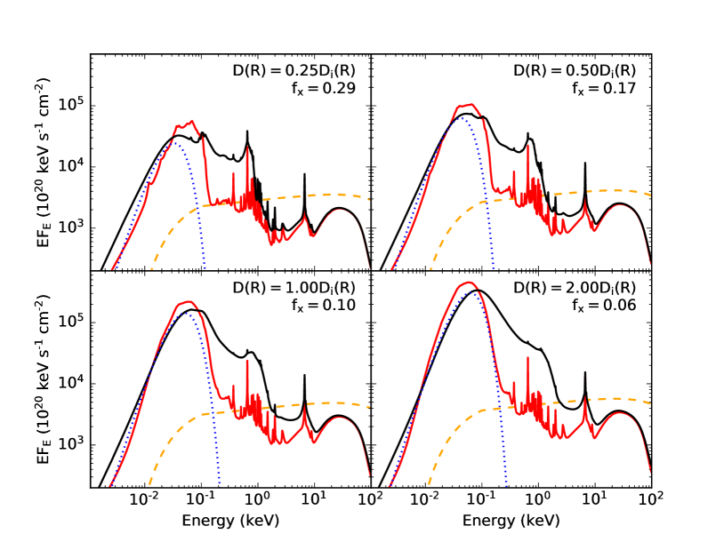
Figure 1: The black lines plot the spectrum emitted from the surface of a constant density slab with $n_{\mathrm{H}}=10^{14}$ cm^-3 and $\tau_{\mathrm{T}}=10$ illuminated by a cutoff power-law from above (dashed orange line) and a blackbody (dotted blue line) from below. A total energy flux $D(R)$ is available to the model, with $f_{\mathrm{X}}D(R)$ going into the external power-law, $h_{f}D(R)$ uniformly injected as heat into the slab (see Eq. 1), and the blackbody taking up the remainder. Each panel in the figure shows the results for $h_{f}=0.3$ when $D(R)$ is varied above and below its initial value ($D_{i}(R)=5.175\times 10^{16}$ erg cm^-2 s^-1) under the assumption $f_{\mathrm{X}}\propto D(R)^{-0.77}$ (Stella & Rosner, 1984). The solid red line in each panel is the spectrum that results with no coronal heating. These plots show that $f_{\mathrm{X}}$ plays a minor role in the ability to maintain a soft excess in an AGN spectrum as $D(R)$ varies.

The figure shows the impact of increasing and decreasing $f_{\mathrm{X}}$ as a result of varying $D(R)$. The top-left panel plots the case where nearly 30% of $D(R)$ is released in the hot corona. Despite the strong external illumination, which corresponds to an ionization parameter ($\xi=4\pi f_{\mathrm{X}}D(R)/n_{\mathrm{H}}$) of $1886$ erg cm s^-1, the surface temperature of the slab is $\approx 0.35$ keV, and Compton cooling does not dominate at any point in the slab. Thus, only a weak soft excess, covered with recombination lines, is produced by this model. As $D(R)$ increases, the flux illuminating the outer surface of the slab falls, but the heating function $\mathcal{H}$ (Eq. 1) grows, releasing more and more energy into the slab. As a result, both the surface temperature and the importance of Compton cooling in the gas increases with $D(R)$, generating a stronger and smoother soft excess in the emitted spectrum. Indeed, when $D(R)/D_{i}(R)=2$, Compton cooling dominates the entire slab and the surface temperature reaches $\approx 1.3$ keV, exceeding the values typically inferred from observations (Petrucci et al., 2018). Clearly, when compared to changes in $\mathcal{H}$, the value of $f_{\mathrm{X}}$ is not important in determining the strength or shape of the soft excess produced by a warm corona. However, the presence of the hard power-law is still required to maintain the base level of surface ionization and avoid strong absorption lines blanketing the emitted spectrum. In the following calculations, we continue to assume $f_{\mathrm{X}}\propto D(R)^{-0.77}$.

3.2 Varying the Density and Thomson Depth

The above experiment indicates that maintaining an appropriate warm corona through changes in an AGN accretion rate must involve the regulation of the coronal heating function, $\mathcal{H}$ (Eq. 1). As found by Ballantyne (2020), if $\mathcal{H}$ is too large or too small, then the warm corona is either too hot or too cold to produce a soft excess consistent with observations. Therefore, other quantities affecting $\mathcal{H}$ must adjust while $D(R)$ changes in order for a warm corona to continuously produce an AGN soft excess.

Models of accretion discs provide some guidance on how discs adjust due to changes in accretion rates. Jiang et al. (2019) ran two global radiation magnetohydrodynamics simulations of AGN discs separated by nearly a factor of 3 in accretion rate. They find that the surface density in the inner part of the disc rises with the accretion rate. As a result, the disc density falls more slowly with height at the larger accretion rate. These results indicate that both the density and optical depth of a heated warm corona might increase in a disc with a larger accretion rate. In addition, Jiang et al. (2019) find that the dissipation fraction in optically thin material is reduced in the higher accretion rate simulation. This result is consistent with the drop in $f_{\mathrm{X}}$ inferred from observations, and could indicate that $h_{f}$, the fraction of accretion powered released in a warm corona, will increase as the accretion rate grows.

To evaluate how the structural changes in the disc found by the simulations will impact maintaining an appropriate warm corona, we calculate the spectra produced by irradiated, heated slabs where $\tau_{\mathrm{T}}\propto D(R)^{3/5}$ and $n_{\mathrm{H}}\propto D(R)^{2/5}$. These relationships are taken from the predictions of gas-pressure dominated $\alpha$-discs (Svensson & Zdziarski, 1994) and both qualitatively follow the same trends with accretion rate suggested by the numerical simulations of Jiang et al. (2019). The baseline model has $D(R)=D_{i}(R)$, $n_{\mathrm{H}}=10^{14}$ cm^-3, $f_{\mathrm{X}}=0.1$, and $\tau_{\mathrm{T}}=8$. This value of $\tau_{\mathrm{T}}$ is consistent with the smallest optical depths inferred for warm coronae (Petrucci et al., 2018). From this baseline model we compute the properties of the slab for $D(R)/D_{i}(R)=1,2,4$ and $8$, with the density, optical depth, and $f_{\mathrm{X}}$ appropriately scaled using the above relationships. In addition, for each value of $D(R)$, the fraction of energy dissipated as heat into the slab, $h_{f}$, is varied from $0.1$ to $0.8$ (in steps of $0.1$) in order to consider a wide range of warm corona properties in each setup.

Figure 2 shows the results from four models, one at each value of $D(R)$, that produce a Compton-dominated warm corona and a smooth soft excess.

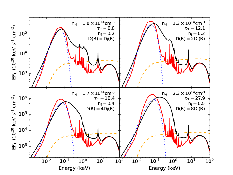
Figure 2: Predictions of the emitted spectrum from an illuminated constant density slab with density $n_{\mathrm{H}}$ and Thomson depth $\tau_{\mathrm{T}}$. In these models, the density, Thomson depth, and fraction of energy released in the hard X-ray power-law ($f_{\mathrm{X}}$) are all functions of the dissipated accretion energy $D(R)$ (see text). The plots show a scenario where $h_{f}$, the fraction of the accretion energy heating the warm corona, increases with $D(R)$ and maintains a Compton dominated soft excess. The line styles are the same as in Figure 1.

The figures show a situation where as $D(R)$ increases, driving growth in both $n_{\mathrm{H}}$ and $\tau_{\mathrm{T}}$, the heating fraction $h_{f}$ also grows to maintain a warm corona with similar properties (see, e.g., Eq. 1). The surface temperatures of the four slabs are not widely different, ranging from $\approx 0.78$ keV for the $D(R)/D_{i}(R)=1$ model (top-left panel) to $\approx 0.9$ keV for the remaining scenarios. The shape of the soft excess predicted in these four models changes significantly as the density and optical depth increases. In the $\tau_{\mathrm{T}}=8$ model, the soft excess still exhibits features due to spectral lines and edges, and shows a modest Compton-scattered continuum formed from the high-energy tail of the blackbody. However, as both $\tau_{\mathrm{T}}$ and $n_{\mathrm{H}}$ increase, the spectral features are erased from the soft excess, and a larger fraction of the blackbody is Compton scattered to form a strong soft excess. This is a result of the blackbody having to pass through a thicker ionized layer as $D(R)$ increases. In fact, the critical optical depth at which Comptonization saturates for a $10$ eV photon passing through a $1$ keV gas is $\tau_{\mathrm{T,crit}}\approx 28$, which is nearly identical to the optical depth used in our models with $D(R)/D_{i}(R)=8$. Thus, we expect that models with larger values of $\tau_{\mathrm{T}}$ will yield spectral shapes similar to the $\tau_{\mathrm{T}}=27.9$ model shown here.

To determine how X-ray observations of AGNs may probe the effects of a changing $n_{\mathrm{H}}$, $\tau_{\mathrm{T}}$ and $h_{f}$ within warm coronae, we add the illuminating power-law to the predicted emitted and reflected spectrum in each model (assuming a reflection fraction of $0.7$; Zappacosta et al. 2018), and calculate the photon index ($\Gamma$) and flux in both the $0.5$–$2$ keV and $2$–$10$ keV bands. The results for models with surface temperatures in the range $0.3$–$1.1$ keV are plotted in Figure 3. These temperatures select warm corona models that span the range found by spectral modeling (e.g., Petrucci et al., 2018).

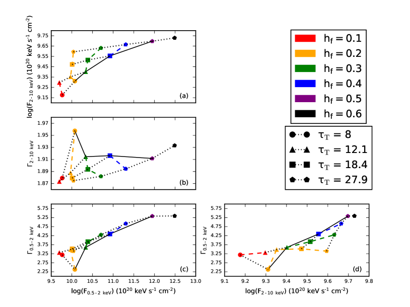
Figure 3: Trends of observational parameters in the X-ray spectra produced by the constant density warm corona models where $\tau_{\mathrm{T}}$, $n_{\mathrm{H}}$ and $f_{\mathrm{X}}$ are all functions of $D(R)$ (see text). Only models with a surface temperature between $0.3$ and $1.1$ keV are included in this analysis to ensure they produce warm coronae consistent with observations (Petrucci et al., 2018). The photon indices and fluxes are calculated from spectra that combine the predicted emission and reflection spectrum (black solid lines in Fig. 2) with the illuminating power-law (dashed lines in Fig. 2), assuming a reflection fraction of $0.7$ (e.g., Zappacosta et al., 2018). The different symbols denote the results from the different $\tau_{\mathrm{T}}$ while the colours indicate the value of $h_{f}$ used in the model. Dotted lines in each panel connect results with the same $\tau_{\mathrm{T}}$, and the coloured dashed lines connect results with the same $h_{f}$. The solid black line in each panel traces out the path of the four models from Fig. 2. The fluxes are calculated in units of emitting area.

In order to isolate the effects of the changing parameters, different symbols are used to indicate warm coronae with different $\tau_{\mathrm{T}}$ and colours are used to distinguish models with different values of $h_{f}$. Dotted lines connect models with equal $\tau_{\mathrm{T}}$ and coloured dashed lines connect models with equal $h_{f}$. An AGN with a soft excess produced by a constant density warm corona will be observed to move through the panels of Fig. 3 on a particular trajectory as its accretion rate changes. For example, the four models shown in Fig. 2 trace out the solid black lines in each panel.

Panel (a) of Fig. 3 plots the predicted $2$–$10$ keV flux versus the $0.5$–$2$ keV flux from the sample of warm coronae. The fluxes are calculated directly from the total spectra and are in units of emitting area. The distribution of points show that warm coronae with a constant $\tau_{\mathrm{T}}$ (dotted lines) are nearly orthogonal in this plane to those with fixed $h_{f}$ (coloured dashed lines). Horizontal movement across the plot is largely driven by increasing $h_{f}$ (i.e., releasing more energy in the warm corona) which enhances the soft flux. In contrast, increases in the hard X-ray flux requires more total energy dissipated in the X-ray power-law, which is most easily achieved by a larger $D(R)$ which, in turn, produces a larger $\tau_{\mathrm{T}}$. However, as $f_{\mathrm{X}}\propto D(R)^{-0.77}$, these changes in $D(R)$ lead to only modest increases in the $2$–$10$ keV flux. Interestingly, strong Comptonization effects when $\tau_{\mathrm{T}}\ga 20$ will also moderately increase the soft flux even if $h_{f}$ is held constant. We conclude that an AGN with a constant density warm corona subject to a variable $h_{f}$ will move horizontally through this flux-flux plot, while changes in $\tau_{\mathrm{T}}$ will cause slight changes in the vertical direction. An example of such a path is shown as the solid black like which is measured from the four spectra shown in Fig. 2.

A similar pattern is seen in Fig. 3(b) which plots $\Gamma_{\mathrm{2-10\ keV}}$ against the soft X-ray flux. The model calculations assume a fixed $\Gamma=1.9$, and only minor changes from this value are observed due to changes in $h_{f}$ and $\tau_{\mathrm{T}}$. The one exception is the $h_{f}=0.2$, $\tau_{\mathrm{T}}=8$ model, shown in the upper-left panel of Fig. 2, as its spectrum is strongly influenced by X-ray reflection features. Consequently, we also expect that constant density warm coronae will move largely horizontally in this plane, driven by changes in $h_{f}$ (solid black line). Changes in the warm corona heating and structural properties will not lead to significant vertical shifts in the plot.

The lower-left panel of Figure 3 shows that soft excesses produced by these constant density warm coronae predict a correlation between $\Gamma_{\mathrm{0.5-2\ keV}}$ and the $0.5$–$2$ keV flux. Basically, as the soft excess gets stronger, it also produces a softer spectrum. As before, the horizontal movement through the plot is driven by the increase in $h_{f}$. A larger $h_{f}$ and $\tau_{\mathrm{T}}$ both yield a softer $\Gamma_{\mathrm{0.5-2\ keV}}$, as each contribute to the importance of Compton cooling in the slabs.

Finally, panel (d) of Fig. 3 shows an interesting separation between low and high $\tau_{\mathrm{T}}$ models in a plot of $\Gamma_{\mathrm{0.5-2\ keV}}$ versus the $2$–$10$ keV flux. As noted above, the hard X-ray flux is primarily affected by $D(R)$, so low $\tau_{\mathrm{T}}$ models are on the left hand side of the plot and more Thomson thick ones are on the right side. Therefore, changes in accretion rate will move an AGN horizontally through this plot. The extent of the vertical motion due to any changes in $h_{f}$ depends on $\tau_{\mathrm{T}}$. Increasing the dissipation in a thick layer enhances Compton cooling, which leads to a softer and stronger soft excess. These effects are weaker for lower values of $\tau_{\mathrm{T}}$ as bremsstrahlung and line-cooling processes can take on larger roles in the cooling of the slab (e.g., Ballantyne, 2020). Indeed, these effects can lead to significant changes in the spectrum when $\tau_{\mathrm{T}}=8$ and the slab is not dominated by Compton cooling. An AGN that has both a variable $\tau_{\mathrm{T}}$ and $h_{f}$ in response to changes to $D(R)$ (e.g., Fig. 2) would then trace out a diagonal path through this plane (black solid line).

In summary, we find that constant density models can maintain appropriate warm coronae (with surface temperatures in the range $0.3$–$1.1$ keV) through changes in $D(R)$ when both the density and optical depth of the corona increase with $D(R)$. In addition, $h_{f}$ will likely also increase with $D(R)$ if the soft excess is to maintained through large increases of $D(R)$. These changes in the structural and heating properties of warm coronae are reflected in the predicted spectral shapes. Comparing the observed changes of AGN soft excesses with the tracks predicted in Fig. 3 will provide an important test for the constant density warm corona model.

3.3 Hydrostatic Models

While useful, constant density slabs are clearly idealizations of the density structure at the surface of accretion discs. Therefore, it is important to consider how a warm corona can be sustained under a more realistic density profile. Ballantyne (2020) showed that the rapidly falling density within a hydrostatic atmosphere will reduce the rate of 2-body cooling processes, and therefore the response of a warm corona to changes in accretion rate could be qualitatively different from the constant density models described above.

We repeat the experiment from Sect. 3.2 with irradiated and heated hydrostatic atmospheres assumed to be at the surface of a radiation-pressure dominated accretion disc (Svensson & Zdziarski, 1994). As before, we define a baseline model with $\tau_{\mathrm{T}}=8$ and $f_{\mathrm{X}}=0.1$, where $\tau_{\mathrm{T}}\propto D(R)^{3/5}$ and $f_{\mathrm{X}}\propto D(R)^{-0.77}$. The density at the base of the atmosphere is initially set by the Svensson & Zdziarski (1994) radiation-pressure dominated disc equations, but the density structure is ultimately determined by requiring the atmosphere to be in hydrostatic balance (Ballantyne et al., 2001). The base densities therefore depend both on $D(R)$ and $h_{f}$, and typically vary over a small range for the models with interesting warm corona with values $\sim 10^{13}$ cm^-3. To compensate for the lower densities, the initial dissipation flux used in the hydrostatic models is set to $D(R)_{i,H}=3.59\times 10^{15}$ erg cm ^-2 s^-1, equivalent to the accretion flux produced at a radius of $5$ Schwarzschild radii around a $3\times 10^{7}$ M_⊙ black hole accreting at $5$% of its Eddington rate. The emission and reflection spectra are then computed for atmospheres with $D(R)/D_{i,H}=1,2$ and $4$, varying $h_{f}$ between $0.1$ and $0.8$ for each value of $D(R)$.

Figure 4 shows three examples of the spectra produced by the irradiated and heated atmospheres, one at each value of $D(R)$, with all producing a strong, smooth soft excess.

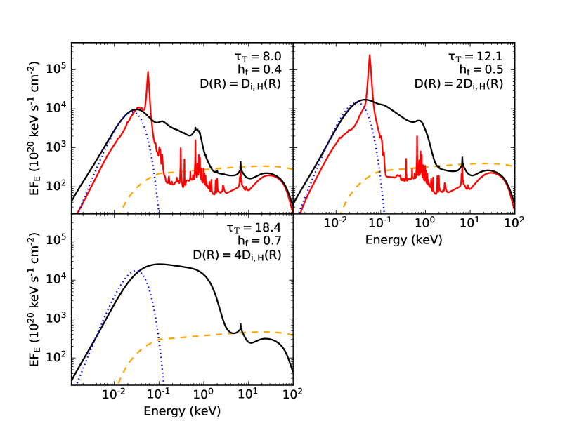
Figure 4: As in Figure 2, but now the modeled layer is a hydrostatic atmosphere at the surface of a radiation-pressure dominated accretion disc (Svensson & Zdziarski, 1994). The baseline accretion flux for this set of calculations is $D_{i,H}(R)=3.59\times 10^{15}$ erg cm² s^-1. The line styles are the same as in Fig. 2. The $\tau_{\mathrm{T}}=18.4$ calculation with no warm coronal heating failed because the gas pressure fell too low at the base of the layer; hence, there is no solid red line in this panel. All three models produce strong soft excesses with the $\tau_{\mathrm{T}}=18.4$ spectrum showing an extreme example of the impact of strong heating in the warm corona. This spectrum is affected by a hot ‘skin’ formed at the surface of the atmosphere which further upscatters the radiation escaping from the atmosphere.

For hydrostatic models, the steep fall off in density with height causes a large increase in coronal heating and gas temperature close to the surface (e.g., Eq. 1). Therefore, it is most useful to examine the properties of the atmospheres at $\tau_{\mathrm{T}}=1$, which occurs close to the transition in the density profile, and is the location which largely determines the properties of the emitted spectrum (e.g., Ballantyne et al., 2001). At this optical depth, the gas temperature is $\approx 0.83$ keV when $D(R)/D_{i,H}(R)=1$, $\approx 0.87$ keV at $D(R)/D_{i,H}(R)=2$ and $\approx 1$ keV when $D(R)/D_{i,H}(R)=4$. All these temperatures are consistent with the warm corona temperatures inferred by Petrucci et al. (2018) from their modeling of XMM-Newton spectra.

The evolution of the soft excess with $D(R)$ in these hydrostatic models appears to follow the same trends as the ones seen in the constant density warm corona (Fig. 2). The soft excess is imprinted with spectral features when $\tau_{\mathrm{T}}=8$ which are then smoothed out at larger optical depths, when Compton cooling processes dominate throughout the atmosphere. However, the spectrum produced by the $\tau_{\mathrm{T}}=18.4$ model in Fig. 4 shows a very extreme soft excess that extends above $2$ keV.

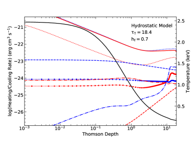
Figure 5: Details on the physical conditions of the $\tau_{\mathrm{T}}=18.4$, $h_{f}=0.7$ hydrostatic warm corona model whose spectrum is shown in the bottom panel of Fig. 4. The red and blue lines show the heating and cooling rates, respectively, as a function of Thomson depth into the atmosphere, and should be read using the left-hand axis. The different processes are denoted by different line styles: Compton heating and cooling (dotted lines), bremsstrahlung heating and cooling (short-dashed lines), photo-ionization heating and line cooling (dot-dashed lines), and recombination heating and cooling (thick dotted lines). The coronal heating function, $\mathcal{H}$ (Eq. 1), is plotted as the solid red line. This rate increases steadily at $\tau_{\mathrm{T}}\la 1$ due to the drop in gas density. The solid black line plots the gas temperature through the atmosphere (read with the right-hand axis). In this model, a Compton dominated warm corona exists throughout the atmosphere, but the strong heating generates a ‘hot skin’ at its surface which provides additional broadening to the emitted spectrum.

As seen in Figure 5, this spectrum is produced by a warm corona that is Compton dominated throughout the atmosphere, but the rapid decline in density leads to a ‘hot skin’ situated at the surface (e.g., Nayakshin & Kallman, 2001). This hot skin provides an additional Compton screen through which deeper emission must pass through. Due to its high temperature, upscattering in the skin smears the emitted spectrum toward higher energies. These extreme soft excesses can only occur in models where a hot skin forms at the disc surface, and therefore are not found in our set of constant density models. As discussed below, the hot skin spectra lead to interesting observational properties.

Figure 6 shows the observational characteristics of the emission and reflected spectra produced by the hydrostatic warm corona models. The layout of the panels is the same as the one for the constant density calculations (Fig. 3).

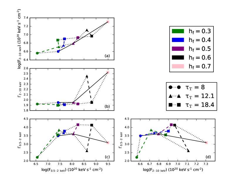
Figure 6: Trends of observational parameters in the X-ray spectra produced by the hydrostatic warm corona models where $\tau_{\mathrm{T}}$ and $f_{\mathrm{X}}$ are functions of $D(R)$. Only models with a temperature at $\tau_{\mathrm{T}}=1$ between $0.3$ and $1.1$ keV are included in this analysis. The photon indices and fluxes are calculated from spectra that combine the predicted emitted/reflected spectrum (black solid lines in Fig. 4) with the illuminating power-law (dashed lines in Fig. 4), assuming a reflection fraction of $0.7$. The different symbols denote the results from the different $\tau_{\mathrm{T}}$ while the colours indicate the value of $h_{f}$ used in the model. Dotted lines in each panel connect results with the same $\tau_{\mathrm{T}}$, and the coloured dashed lines connect results with the same $h_{f}$. The three models shown in Fig. 4 follow the solid black line in each panel. The fluxes are calculated in units of emitting area.

The hydrostatic atmospheres plotted in the Figure are selected to all have temperatures at $\tau_{\mathrm{T}}=1$ between $0.3$ and $1.1$ keV to ensure they bracket the inferred properties of warm absorbers (e.g. Petrucci et al., 2018). As in Fig. 3, the measurements are made from spectra that have a reflection fraction of $0.7$.

Many of the trends observed in Fig. 6 are similar to the ones in Fig. 3. For example, in panel (a), horizontal motion across the figure is driven by increasing $h_{f}$, while increases in the $2$–$10$ keV flux, which drives vertical motion, is largely achieved by increasing $D(R)$ (and, hence, larger $\tau_{\mathrm{T}}$). However, there are two interesting exceptions. The first is a significant increase in the soft X-ray flux in the $\tau_{\mathrm{T}}=8$ models when $h_{f}$ is changed from $0.3$ to $0.4$ due to the development of a Compton cooled warm corona. The second exception is the large jump in $F_{\mathrm{2-10\ keV}}$ due to the $h_{f}=0.7$, $\tau_{\mathrm{T}}=18.4$ model (bottom spectrum in Fig. 4). The extreme soft excess in that spectrum actually extends above $2$ keV enhancing the flux in the hard X-ray band. An AGN that is subject to significant heating in the warm corona may therefore trace a steep trajectory in this flux-flux plane (e.g., the solid black line, which follows the three models shown in Fig. 4).

The hard X-ray photon index, $\Gamma_{\mathrm{2-10\ keV}}$, predicted by the hydrostatic warm corona models is relatively insensitive to the affects of the corona heating (Fig. 6(b)), with values close to the input slope of $1.9$. This result is consistent with the results of the constant density models (Fig 3). Interestingly, there are two significant outliers to this trend which both show $\Gamma_{\mathrm{2-10\ keV}}\approx 2.5$. These two warm corona generate extreme soft excesses that extends to energies $>2$ keV due to the formation of a ‘hot skin’ that upscatters the emitted radiation field (e.g., the bottom panel of Fig. 4). Thus, even though the irradiating power law has a $\Gamma=1.9$, the inferred $\Gamma_{\mathrm{2-10\ keV}}$ would be significantly steeper.

Panel (c) of Fig. 6 shows a more complex relationship between $\Gamma_{\mathrm{0.5-2\ keV}}$ and $F_{\mathrm{0.5-2\ keV}}$ for the hydrostatic warm coronae than shown in Fig. 3(c) for the constant density models. We again see a correlation between the photon index and the soft X-ray flux that traces the development of a Compton cooled warm corona. Once this is established, then increases in $h_{f}$ only changes $\Gamma_{\mathrm{0.5-2\ keV}}$ by a small amount until the temperature of the warm corona increases to the point that the hot skin forms and contributes to the soft excess. Once this stage is achieved, the soft X-ray photon index begins to drop with X-ray flux, as the shape of the spectrum is flattened by Comptonization in the hot skin. Thus, an AGN that follows a declining trajectory in this plane may be showing evidence for the development of a strongly heated warm corona (e.g., the solid black line in panel (b)).

A similar effect is seen in the final panel of Fig. 6 which plots $\Gamma_{\mathrm{0.5-2\ keV}}$ against the $2$–$10$ keV flux calculated from the hydrostatic warm corona models. There is little change in $\Gamma_{\mathrm{0.5-2\ keV}}$ once a Compton cooled warm corona develops, but a large change in the photon index and $F_{\mathrm{2-10\ keV}}$ occurs when an extreme soft excess is produced by strong coronal heating. As described above (and seen in the bottom panel of Fig. 4), the soft excess in this case is impacted by Comptonization in a hot skin that flattens the soft X-ray spectrum and extends it into the hard X-ray band. Thus, these models will lead to an increase in $F_{\mathrm{2-10\ keV}}$ accompanied by a drop in $\Gamma_{\mathrm{0.5-2\ keV}}$. This change in slope occurs faster when coronal heating increases in atmospheres with smaller $\tau_{\mathrm{T}}$ (comparing the triangles to the squares in the panel (d)).

The above results show that a strong soft excess produced by a hydrostatic warm corona can be sustained through large changes in dissipated flux by appropriate increases in the optical depth and $h_{f}$. The rapidly declining density structure of the hydrostatic atmosphere allows the production of more extreme soft excesses when the coronal heating is large. These soft excesses still have temperatures at $\tau_{\mathrm{T}}=1$ of $\sim 1$ keV but produce a broader and flatter soft excess (due to Comptonization in a hot skin) that extends above $2$ keV. The resulting spectra will be observed to have a steep $\Gamma_{\mathrm{2-10\ keV}}$, and their development will lead to negative correlations between $\Gamma_{\mathrm{0.5-2\ keV}}$ and the observed soft and hard fluxes.

4 Discussion

Recent work by Ballantyne (2020) and Petrucci et al. (2020) have shown that a warm corona with $\tau_{\mathrm{T}}\approx 10$–$20$ at the surface of an accretion disc can, under certain conditions, produce a strong, smooth soft excess that is qualitatively consistent with observations. This paper explores the question of how the warm corona and heating properties change in order to sustain the soft excess while the underlying accretion flux, $D(R)$, varies. The results shown above show that maintaining a warm corona of the right properties can be accomplished if $\tau_{\mathrm{T}}$, and, to a lesser extent, $n_{\mathrm{H}}$ increases with $D(R)$. The fraction of accretion energy dissipated in the warm corona, $h_{f}$, may also change with $D(R)$, depending on the value of $\tau_{\mathrm{T}}$. The range of possible $h_{f}$ that yields a warm corona is narrower for smaller $\tau_{\mathrm{T}}$. Thus, it is easier to maintain a warm corona when $\tau_{\mathrm{T}}$ is large (e.g., Fig. 3). In this section, we compare the results shown in Sect. 3 to recent observations measuring changes in AGN soft excesses. As the warm coronae models are calculated only at a single disc radius, the comparison to observations will necessarily be qualitative. Model accretion disc spectra incorporating both a hard X-ray power-law and a warm corona is planned for future work.

Figures 3 and 6 show how the observed properties of soft excesses predicted by the warm corona models vary with flux. These soft excesses are produced by the combination of Comptonized blackbody emission passing through the warm corona, plus bremsstrahlung and recombination line radiation due to illumination from the external hard X-ray power-law. Both panels assume the final spectrum has a fixed reflection fraction of $0.7$. Figure 3 shows the changes in the soft excess as the warm corona properties are modified to be sustained over a factor of 8 increase in $D(R)$. The soft excess grows stronger and softer as the accretion flux increases, with the strength of the dependence varying on the details of $h_{f}$ (e.g., Fig. 3). However, these changes often have a very minor effect on the shape of the $2$–$10$ keV spectrum. In contrast, Fig. 6 shows how a strongly heated warm corona can produce an extreme soft excess that extends above $2$ keV. In this scenario, the stronger and softer relationships seen in the previous case inverts, and the spectrum becomes both harder on the soft band and softer in the hard band with a $\Gamma_{\mathrm{2-10\ keV}}\approx 2.5$. These extreme soft excesses are produced in strongly heated hydrostatic atmosphere due to the formation of a hot skin at the surface which further Compton upscatters the emitted spectrum. The hard X-ray spectra of many AGNs appear to soften as their flux increases (e.g., Keek & Ballantyne, 2016), and there is tentative evidence that $\Gamma_{\mathrm{2-10\ keV}}$ is correlated with the Eddington ratio (e.g., Trakhtenbrot et al., 2017). The formation of this hot skin and its dependence on $h_{f}$ is a possible explanation for these relationships. If more accretion energy is dissipated in a warm corona at larger Eddington ratios than a ‘hot skin’ will also develop at larger accretion rates. Comptonization in this hot skin will steepen the observed $2$–$10$ keV spectrum, independent of the shape of the illuminating power-law. The effectiveness of the process will depend on the details of the heating in both the warm and hot coronae, and could naturally account for the observed scatter in the relationships between photon index and Eddington ratio. The impact of the extreme soft excess on the spectrum will be less important at energies $\ga 10$ keV, and the spectrum will appear to harden at these energies. Therefore, a power-law fit to such a spectrum (e.g., one observed by NuSTAR) will return a large reflection fraction. AGNs with steep power-laws and strong reflection fractions (e.g., Jiang et al., 2018) may therefore be explained by a strongly heated hydrostatic warm corona.

AGNs with soft excesses will trace out trajectories through the panels of Figs. 3 and 6. By comparing these trajectories to the different relationships plotted in the figures, we can determine if these trajectories are consistent with a warm corona model that has a constant $\tau_{\mathrm{T}}$ or $h_{f}$, or one that has a variable structure. For example, Ursini et al. (2020) recently studied five joint XMM-Newton and NuSTAR observations of the ‘bare’ Seyfert 1 galaxy HE 1143-1810. All five observations of the AGN show a strong soft excess, and the five observations span a factor of $\approx 2$ in flux. Ursini et al. (2020) considered a two corona model that includes emission from both a hot and warm Comptonizing corona. The authors found that the photon index of the warm corona was anti-correlated with the soft flux, and there was also a correlation between the hard and soft fluxes. A correlation between the soft and hard band fluxes is a common prediction of the warm corona models described here, with a shallow slope for a constant $\tau_{\mathrm{T}}$, and a steeper one if $\tau_{\mathrm{T}}$ is changing (e.g., Fig. 6(a)). Interestingly, an anti-correlation between the soft photon index and soft flux is only seen in Fig. 6(c) when $\tau_{\mathrm{T}}$ is constant and $h_{f}$ is increasing (e.g., the triangles in Fig. 6(c)). Ursini et al. (2020) note that there is very little change in the inferred $\tau_{\mathrm{T}}$ of the warm corona between the low and high flux states (with $\tau_{\mathrm{T}}\approx 17$–$18$). Therefore, qualitatively, the soft excess of HE 1143-1810 is consistent with a hydrostatic warm corona at a fixed $\tau_{\mathrm{T}}$ with $h_{f}$ increasing with flux.

Similar results were found by Middei et al. (2019) who analyzed 5 XMM-Newton and NuSTAR observations of the Seyfert galaxy NGC 4593 with a two corona model. These data spanned approximately a factor of 2 in flux, and Middei et al. (2019) determined that the soft X-ray photon index was anti-correlated with the hard X-ray ($2$–$10$ keV) flux, but, as with HE 1143-1810, the hard and soft band fluxes were correlated. Fig. 6(a) and (d) indicate that evolution at a fixed $\tau_{\mathrm{T}}$ is consistent with these trends. Interestingly, Middei et al. (2019) also find an anti-correlation between the photon indices of the soft and hard components.

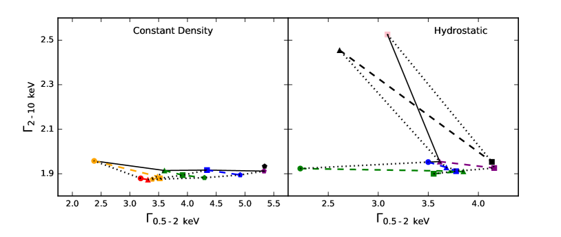
Figure 7: Potential relationships between the hard and soft X-ray photon indices measured from the constant density (left-hand panel) and hydrostatic (right-hand panel) warm corona models. The plotted points and lines are the same as the ones from Figs. 3 and 6. The constant density warm corona models with temperatures between $0.3$ and $1.1$ keV produce only very small changes in $\Gamma_{\mathrm{2-10\ keV}}$, even if the soft X-ray photon index varies significantly. In contrast, if a hot skin forms on the surface of a hydrostatic model (e.g., Fig. 5), then this will significantly alter the observed $\Gamma_{\mathrm{2-10\ keV}}$, even though the spectrum emitted by the hot corona is unchanged.

Fig. 7 shows that no relationship between the photon indices is found from the constant density warm corona models with surface temperatures of $0.3$–$1.1$ keV, despite large changes in $\Gamma_{\mathrm{0.5-2\ keV}}$ due to an increasing soft excess. However, an anti-correlation between the two photon-indices can be seen in hydrostatic warm coronae with a fixed $\tau_{\mathrm{T}}$ (right-hand panel of Fig. 7), due to the development of the ‘hot skin’ at the surface of the atmosphere (e.g., Fig. 5). Although a quantitative comparison is not yet possible, such an anti-correlation may be an indication of a changing coronal heating fraction. However, Middei et al. (2019) do not find any correlations (neither positive nor negative) between the soft photon index and the soft X-ray flux. Given the other observed correlations seen from this AGN, it is challenging to explain this lack of correlation with the simple warm corona models considered here. Clearly, there is a need for models that encompasses a larger fraction of the accretion disc with which to compare against observations.

A common observational measurement of the strength of a soft excess in the spectrum of an AGN is SX1, which is defined as the $0.5$–$2$ keV flux of a blackbody fit to the soft excess, divided by the flux of the hard X-ray power-law extrapolated into the same band. This parameter therefore gives an estimate of the amount of ‘excess’ flux above what is expected from the hard X-ray power-law. A recent analysis by Gliozzi & Williams (2020) of 89 type-1 AGNs find that SX1 tends to be larger for more rapidly accreting AGNs, such as narrow-line Seyfert 1 galaxies, albeit with a large amount of scatter. To see if the soft excesses produced by the warm corona models also show a similar trend we compute

$$\mathrm{SX1}=\left({F^{\mathrm{refl}}_{\mathrm{0.5-2\ keV}}\over F^{\mathrm{pl}}_{\mathrm{0.5-2\ keV}}}\right),$$ (2)

where $F^{\mathrm{refl}}_{\mathrm{0.5-2\ keV}}$ is the $0.5$–$2$ keV flux of the emission/reflection spectrum emitted by the warm corona (i.e., the black lines in Figs. 2 and 4), and $F^{\mathrm{pl}}_{\mathrm{0.5-2\ keV}}$ is the $0.5$–$2$ keV flux of the power-law (i.e., the orange dashed lines in the same figures). We compute SX1 for all the constant density and hydrostatic warm corona models plotted in Figs. 3 and 6. In agreement with Gliozzi & Williams (2020), Figure 8 shows that SX1 is correlated with $D(R)$, the dissipated accretion energy which is proportional to the AGN accretion rate.

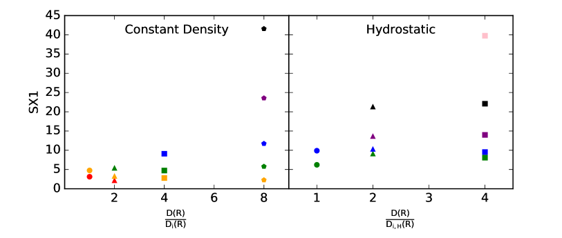
Figure 8: (Left) Plot of SX1 (Eq. 2) versus $D(R)/D_{i}(R)$ for the constant density warm corona models shown in Fig. 3. The colours and shapes of the points are the same as in that Figure. (Right) As in the other panel, but now for the hydrostatic warm corona models shown in Fig. 6. In both cases, the value of SX1 can vary significantly at a given accretion flux, depending on the value of $h_{f}$. This is consistent with observations showing a loose correlation between the strength of an AGN soft excess and its Eddington ration (e.g., Gliozzi & Williams, 2020).

Furthermore, warm corona models naturally explain the large observed scatter in the relationship as the coronal heating fraction $h_{f}$ can vary significantly from source to source. Because a broader range of $h_{f}$ is allowable in warm coronae with larger $D(R)$ (i.e., a larger $\tau_{\mathrm{T}}$), then the scatter of SX1 values is larger at higher accretion rates, than at lower ones, in agreement with the results of Gliozzi & Williams (2020). Therefore, warm coronae with $\tau_{\mathrm{T}}$ correlated with the accretion rate (and a variable $h_{f}$), appear to be a viable explanation for the observed trends in the soft excess strength.

5 Conclusions

Any model explaining the origin of the soft excess in AGNs must be able to account for its ubiquity, its persistence to changes in luminosity, and both its short and long time-scale variability. A soft excess produced by a combination of a warm corona and reflected emission has many qualities consistent with these properties. Reflection from an external hard X-ray power-law will naturally produce a soft excess that can then be strengthened and smoothed by Comptonized thermal emission from a warm corona. Thus, as long as the hard X-ray and optically thick accretion disc are present, a soft excess should be a common feature in AGNs. As shown above, variations in the external X-ray flux, and, in particular, in the structure and heating of the warm corona, will sustain the soft excess through changes in the underlying accretion rate, and drive variations in the observed spectra (e.g., Figs. 3 and 6). AGN observing campaigns that trace the changes in the soft excess spectral properties with flux will be able to constrain the heating properties of the warm corona. For example, comparing the warm corona models with the soft excess changes seen in HE 1143-1810 (Ursini et al., 2020) and NGC 4593 (Middei et al., 2019) indicates that a variable heating fraction in a hydrostatic warm corona is the primary driver of the observed changes. More rigorous results will be obtained by using datasets that span a larger range of flux variations, perhaps by exploiting archival data.

Significant work remains in order to determine if warm coronae are an important contributor to the soft excess of all AGNs, or are only relevant for a smaller population of sources (e.g., those that exhibit ionized Fe K$\alpha$ lines). The one-dimensional models described here and by Petrucci et al. (2020) need to be extended to account for emission from a larger fraction of the accretion disc before a rigorous comparison to AGN spectra can be performed. Similarly, additional theoretical and numerical work on the structure and heating of the outermost layers of accretion flows is needed to inform the construction of spectral models such as the ones presented in this paper. For example, magnetic heating (e.g., Gronkiewicz & Różańska, 2020) will provide a different vertical heating profile than the uniform heating function used here (Eq. 1), and could affect how changes in the warm corona impact the emitted spectrum.

Our results show that the combination of a warm corona and hard X-ray reflection produce a diversity of soft excess shapes and strengths. Changes to the density, optical depth and/or coronal heating strength will sustain a soft excess through large changes in accretion rate. Overall, our results reinforce the idea that not only can a warm corona be an important contributor to the AGN soft excess, but also illustrates how observations of the soft excess can provide new insights into the physics of accretions discs around black holes.

Data Availability

The data underlying this article will be shared on reasonable request to the corresponding author.

References

- Ballantyne (2017) Ballantyne D. R., 2017, MNRAS, 472, L60
- Ballantyne (2020) Ballantyne D. R., 2020, MNRAS, 491, 3553
- Ballantyne et al. (2001) Ballantyne D. R., Ross R. R., Fabian A. C., 2001, MNRAS, 327, 10
- Ballantyne et al. (2002) Ballantyne D. R., Ross R. R., Fabian A. C., 2002, MNRAS, 336, 867
- Bianchi et al. (2009) Bianchi S., Guainazzi M., Matt G., Fonseca Bonilla N., Ponti G., 2009, A&A, 495, 421
- Crummy et al. (2006) Crummy J., Fabian A. C., Gallo L., Ross R. R., 2006, MNRAS, 365, 1067
- Czerny et al. (2003) Czerny B., Nikołajuk M., Różańska A., Dumont A. M., Loska Z., Zycki P. T., 2003, A&A, 412, 317
- De Marco & Ponti (2019) De Marco B., Ponti G., 2019, Astronomische Nachrichten, 340, 290
- Duras et al. (2020) Duras F., et al., 2020, A&A, 636, A73
- Elvis et al. (1994) Elvis M., et al., 1994, ApJS, 95, 1
- Fabian & Ross (2010) Fabian A. C., Ross R. R., 2010, Space Sci. Rev., 157, 167
- Fabian et al. (2017) Fabian A. C., Lohfink A., Belmont R., Malzac J., Coppi P., 2017, MNRAS, 467, 2566
- Frank et al. (2002) Frank J., King A., Raine D. J., 2002, Accretion Power in Astrophysics: Third Edition. Cambridge University Press
- Galeev et al. (1979) Galeev A. A., Rosner R., Vaiana G. S., 1979, ApJ, 229, 318
- García et al. (2013) García J., Dauser T., Reynolds C. S., Kallman T. R., McClintock J. E., Wilms J., Eikmann W., 2013, ApJ, 768, 146
- García et al. (2019) García J. A., et al., 2019, ApJ, 871, 88
- Gierliński & Done (2004) Gierliński M., Done C., 2004, MNRAS, 349, L7
- Gliozzi & Williams (2020) Gliozzi M., Williams J. K., 2020, MNRAS, 491, 532
- Gronkiewicz & Różańska (2020) Gronkiewicz D., Różańska A., 2020, A&A, 633, A35
- Haardt & Maraschi (1991) Haardt F., Maraschi L., 1991, ApJ, 380, L51
- Haardt & Maraschi (1993) Haardt F., Maraschi L., 1993, ApJ, 413, 507
- Jiang et al. (2018) Jiang J., et al., 2018, MNRAS, 477, 3711
- Jiang et al. (2019) Jiang Y.-F., Blaes O., Stone J. M., Davis S. W., 2019, ApJ, 885, 144
- Kara et al. (2016) Kara E., Alston W. N., Fabian A. C., Cackett E. M., Uttley P., Reynolds C. S., Zoghbi A., 2016, MNRAS, 462, 511
- Keek & Ballantyne (2016) Keek L., Ballantyne D. R., 2016, MNRAS, 456, 2722
- Kubota & Done (2018) Kubota A., Done C., 2018, MNRAS, 480, 1247
- Liu et al. (2017) Liu T., et al., 2017, ApJS, 232, 8
- Lobban et al. (2018) Lobban A. P., Vaughan S., Pounds K., Reeves J. N., 2018, MNRAS, 476, 225
- Magdziarz et al. (1998) Magdziarz P., Blaes O. M., Zdziarski A. A., Johnson W. N., Smith D. A., 1998, MNRAS, 301, 179
- Mallick et al. (2018) Mallick L., et al., 2018, MNRAS, 479, 615
- Middei et al. (2019) Middei R., et al., 2019, MNRAS, 483, 4695
- Nayakshin & Kallman (2001) Nayakshin S., Kallman T. R., 2001, ApJ, 546, 406
- Netzer (2019) Netzer H., 2019, MNRAS, 488, 5185
- Petrucci et al. (2001) Petrucci P. O., et al., 2001, ApJ, 556, 716
- Petrucci et al. (2018) Petrucci P. O., Ursini F., De Rosa A., Bianchi S., Cappi M., Matt G., Dadina M., Malzac J., 2018, A&A, 611, A59
- Petrucci et al. (2020) Petrucci P. O., et al., 2020, A&A, 634, A85
- Reis & Miller (2013) Reis R. C., Miller J. M., 2013, ApJ, 769, L7
- Ricci et al. (2017) Ricci C., et al., 2017, ApJS, 233, 17
- Ricci et al. (2018) Ricci C., et al., 2018, MNRAS, 480, 1819
- Ross (1979) Ross R. R., 1979, ApJ, 233, 334
- Ross & Fabian (1993) Ross R. R., Fabian A. C., 1993, MNRAS, 261, 74
- Scott et al. (2012) Scott A. E., Stewart G. C., Mateos S., 2012, MNRAS, 423, 2633
- Shakura & Sunyaev (1973) Shakura N. I., Sunyaev R. A., 1973, A&A, 500, 33
- Stella & Rosner (1984) Stella L., Rosner R., 1984, ApJ, 277, 312
- Svensson & Zdziarski (1994) Svensson R., Zdziarski A. A., 1994, ApJ, 436, 599
- Trakhtenbrot et al. (2017) Trakhtenbrot B., et al., 2017, MNRAS, 470, 800
- Ursini et al. (2020) Ursini F., et al., 2020, A&A, 634, A92
- Vasudevan & Fabian (2007) Vasudevan R. V., Fabian A. C., 2007, MNRAS, 381, 1235
- Walter & Fink (1993) Walter R., Fink H. H., 1993, A&A, 274, 105
- Winter et al. (2012) Winter L. M., Veilleux S., McKernan B., Kallman T. R., 2012, ApJ, 745, 107
- Zappacosta et al. (2018) Zappacosta L., et al., 2018, ApJ, 854, 33