Pseudospectral approximation of Hopf bifurcation for delay differential equations

Abstract

Pseudospectral approximation reduces DDE (delay differential equations) to ODE (ordinary differential equations). Next one can use ODE tools to perform a numerical bifurcation analysis. By way of an example we show that this yields an efficient and reliable method to qualitatively as well as quantitatively analyse certain DDE. To substantiate the method, we next show that the structure of the approximating ODE is reminiscent of the structure of the generator of translation along solutions of the DDE. Concentrating on the Hopf bifurcation, we then exploit this similarity to reveal the connection between DDE and ODE bifurcation coefficients and to prove the convergence of the latter to the former when the dimension approaches infinity.

AMS Subject Classification: 34K18, 37M20, 65P30, 65L03, 92D25

1 Introduction

Numerical bifurcation analysis [20, 24] is nowadays a powerful method for analysing dynamical systems that arise in applications. For ordinary differential equations (ODE) trustworthy tools, such as Auto [1] and MatCont [10], exist (here ‘trustworthy’ indicates that they are tested and maintained, i.e., adapted when the software or hardware environment in which they are embedded changes). For delay differential equations (DDE) there are trustworthy tools too, e.g., DDE-BIFTOOL [17, 18] and KNUT [2], but these can handle only specific classes of DDE, such as equations with point delays, and it seems fair to say that both maintenance and testing is somewhat vulnerable, because it relies on the efforts of just a few individuals, if not just one. So if we manage to systematically approximate infinite dimensional dynamical systems corresponding to DDE by finite dimensional systems corresponding to ODE, we may lose some precision in the numerical bifurcation analysis, but we would be able to handle a much larger class of equations.

In [6] pseudospectral approximation is advocated as a promising approach to achieve exactly this. The aim of the present paper is to make a next step by verifying that the generic Hopf bifurcation in DDE is faithfully captured by Hopf bifurcations in the approximating ODE systems. Our theoretical results concern the limit when the dimension of the approximating system goes to infinity. In practice we of course at best verify that a bifurcation diagram remains essentially unchanged when the dimension is increased by a finite amount (for example doubled). The theoretical results generate confidence that the bifurcation diagram of the approximating ODE captures the DDE dynamics if it is robust under increase of the dimension.

In the following we take a famous example from mathematical biology, namely the ‘Nicholson’s blowflies’ equation, as a testing ground to illustrate some features of the approach. However, we remark that the methodology presented here (pseudospectral approximation combined with software for bifurcation analysis of ODE) can be applied in a much more general setting: it is indeed a promising procedure to study differential equations with distributed, state-dependent, and even infinite delays [6, 22, 19], as well as nonlinear renewal equations [7] and first order partial differential equations [31]. The advantage of considering Nicholson’s blowflies equation in this context is due to the fact that explicit comparisons are possible, both with analytically computed quantities and with alternative numerical approximations, as will become clear later on.

2 A motivating example: ‘Nicholson’s blowflies’ equation

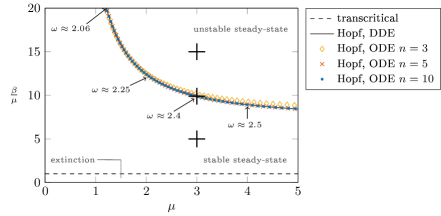
Figure 1: Stability diagram of (2.1) and its pseudospectral approximation for $\tau=1$ and $h(x)=e^{-x}$. The horizontal black dashed line indicates the transcritical bifurcation in (2.1) and its pseudospectral approximation. The Hopf bifurcation curves are computed analytically, both for the DDE (black solid) and the pseudospectral approximation (colors), see Appendix. The different values of $\omega$ indicated along the Hopf bifurcation curve specify the position of the critical root of the characteristic equation on the positive imaginary axis. The black crosses refer to parameter values used in Figure 2.

In the paper [21], Gurney, Blythe and Nisbet showed that Nicholson’s classic laboratory blowfly data are in good quantitative agreement with various characteristics of solutions of the DDE

$$N^{\prime}(t)=-\mu N(t)+\beta N(t-\tau)h(N(t-\tau)),\quad t\geq 0.$$ (2.1)

Here $N$ corresponds to the size of the population of adults, where newborns become adult after a maturation delay $\tau$. The parameter $\mu\geq 0$ refers to the per capita death rate and $\beta\geq 0$ to the maximum per capita egg production rate. The graph of the recruitment function $N\mapsto Nh(N)$ is assumed to be humped. This form reflects scramble competition for the experimentally controlled limited amount of protein resource: female adults need a certain quantity of protein in order to be able to produce eggs.

So (2.1) has a very respectable background in population biology. Here we want to demonstrate that the pseudospectral methodology enables a quick and efficient numerical bifurcation analysis of (2.1) with relatively little effort. In addition we shall pay attention to the accuracy of the approximation. Equation (2.1) is rather well suited to do so, as several features (in particular the stability boundary in a two-parameter space, see Figure 1) can be derived analytically.

Using the pseudospectral technique, equation (2.1) is approximated by a system of $n+1$ ODE for the variables $y_{0},\dots,y_{n}$, where the first equation reads

$$y_{0}^{\prime}=-\mu y_{0}+\beta y_{n}h(y_{n}),$$ (2.2)

and captures the rule for extension (2.1), with $y_{0}(t)$ and $y_{n}(t)$ approximating $N(t)$ and $N(t-\tau)$, respectively. The remaining $n$ equations are needed to describe translation along the solution, and are in fact independent of the specific delay equation. We refer to Section 4 for the details of the pseudospectral approximation.

Under the assumption that $h$ is decreasing and vanishing at infinity, with $h(0)=1$, for every $\beta>\mu$ there exists a positive equilibrium of both equation (2.1) and the corresponding approximating system. Moreover, for both equations the stability boundary (in a two-parameter plane) of the positive equilibrium can be computed analytically. We shall do so in Appendix A.

We find that for $\beta<\mu$ the trivial equilibrium is asymptotically stable and the population goes extinct. For $\beta=\mu$ the trivial and non-trivial equilibrium exchange stability in a transcritical bifurcation. If we then follow a one-parameter path in the $(\mu,\beta/\mu)$-plane that crosses the Hopf bifurcation curve (see Figure 1) transversally, the positive equilibrium of (2.1) loses its stability in a Hopf bifurcation. Figure 1 gives the stability diagram for (2.1) and its pseudospectral approximation, for various values of the discretisation parameter $n$.

One of the main advantages of the pseudospectral approximation is that the resulting system can be analysed with software for the numerical bifurcation analysis of ODE. Throughout the following sections, we will illustrate the obtained results by comparing analytical computations for (2.1) with numerical bifurcation results of the approximating ODE. In Section 8 we will explore the dynamics beyond the Hopf bifurcation curve and show that, using numerical approximations, one can transcend a pen-and-paper analysis and investigate more complex objects like periodic solutions and their bifurcations.

In the following sections we will study the convergence of the approximations in the limit $n\to\infty$. In this perspective, Figure 1 and later figures lift up our spirits by showing that, in practice, the approximation of the stability curves and associated quantities is extremely good already for low values of $n$.

3 The Hopf bifurcation theorem: a quick refresher

In this section, we recall the Hopf bifurcation theorem for general ODE and for scalar DDE. For proofs of (equivalent formulations of) the results, as well as additional references, see [14, Chapter X, Theorems 2.1, 2.7, 3.1 and 3.9] and [25].

Consider the ODE

$$x^{\prime}(t)=A(\alpha)x(t)+f(x(t),\alpha),\qquad t\geq 0$$ (3.1)

with $\alpha\in\mathbb{R}$, $A(\alpha):\mathbb{R}^{d}\to\mathbb{R}^{d}$ linear and $f:\mathbb{R}^{d}\times\mathbb{R}\to\mathbb{R}^{d}$ for some $d\in\mathbb{N}$. We summarise the relevant requirements on $A$ and $f$ in a hypothesis.

Hypothesis 1.

1. $f:\mathbb{R}^{d}\times\mathbb{R}\to\mathbb{R}^{d}$ and $\alpha\mapsto A(\alpha)$ are $C^{k}$ smooth for some $k\geq 3$;

2. $f(0,\alpha)=0$ and $D_{1}f(0,\alpha)=0$ for all $\alpha\in\mathbb{R}$.

Under this hypothesis, system (3.1) has an equilibrium $x=0$ for all $\alpha\in\mathbb{R}$, but in the results presented below only a small neighbourhood of a specific value $\alpha_{0}$ matters. The linearisation of (3.1) at this equilibrium is given by

$$\dot{x}(t)=A(\alpha)x(t).$$

For two vectors $v,w\in\mathbb{C}^{d}$, we define

$$v\cdot w=\sum_{i=1}^{n}v_{i}w_{i}.$$

Note that this differs from the inner product between $v$ and $w$, which is $v\cdot\overline{w}$ (or $\overline{v}\cdot w$) in the present notation.

Theorem 3.1 (Hopf bifurcation theorem for ODE).

Consider system (3.1) and assume that Hypothesis 1 is satisfied. If there exist $\alpha_{0}\in\mathbb{R}$ and $\omega_{0}>0$ such that

1. $i\omega_{0}$ is a simple eigenvalue of $A(\alpha_{0})$;

2. the branch of eigenvalues of $A(\alpha)$ through $i\omega_{0}$ at $\alpha=\alpha_{0}$ intersects the imaginary axis transversally, i.e., the real part of the derivative of the eigenvalues along the branch is non-zero. If we denote by $p,q\in\mathbb{C}^{d}\backslash\{0\}$ vectors such that $A(\alpha_{0})p=i\omega_{0}p,\ A(\alpha_{0})^{T}q=i\omega_{0}q$ and $q\cdot p=1$, then this condition amounts to

   $$\mbox{Re}\,\left(q\cdot A^{\prime}(\alpha_{0})p\right)\neq 0;$$ (3.2)

3. $ki\omega_{0}$ is not an eigenvalue of $A(\alpha_{0})$ for $k=0,2,3,\ldots$

then a Hopf bifurcation occurs for $\alpha=\alpha_{0}$. This means that there exist $C^{k-1}$ functions $\epsilon\mapsto\alpha^{\ast}(\epsilon),\ \epsilon\mapsto\omega^{\ast}(\epsilon)$ taking values in $\mathbb{R}$ and $\epsilon\mapsto x^{\ast}(\epsilon)\in{\color[rgb]{0,0,0}C_{b}(\mathbb{R},\mathbb{R}^{d})}$, all defined for $\epsilon$ sufficiently small, such that for $\alpha=\alpha^{\ast}(\epsilon)$, $x^{\ast}(\epsilon)$ is a periodic solution of (3.1) with period $2\pi/\omega^{\ast}(\epsilon)$. Moreover, $\alpha^{\ast}$ and $\omega^{\ast}$ are even functions, $\alpha^{\ast}(0)=\alpha_{0},\ \omega^{\ast}(0)=\omega_{0}$ and if $x$ is a small periodic solution of (3.1) for $\alpha$ close to $\alpha_{0}$ and minimal period close to $2\pi/\omega_{0}$, then $x(t)=x^{\ast}(\epsilon)(t+\theta^{\ast})$ and $\alpha=\alpha^{\ast}(\epsilon)$ for some $\epsilon$ and some $\theta^{\ast}\in[0,2\pi/\omega^{\ast}(\epsilon))$.

Moreover, $\alpha^{\ast}$ has the expansion $\alpha^{\ast}(\epsilon)=\alpha_{0}+a_{20}\epsilon^{2}+o(\epsilon^{2})$, with $a_{20}$ given by

$$a_{20}=-\frac{\mbox{Re}\,c}{\mbox{Re}\,\left(q\cdot A^{\prime}(\alpha_{0})p\right)}$$

with

$$c= \frac{1}{2}q\cdot D_{1}^{3}f(0,\alpha_{0})(p,p,\overline{p})+q\cdot D_{1}^{2}f(0,\alpha_{0})\bigl{(}-A(\alpha_{0})^{-1}D_{1}^{2}f(0,\alpha_{0})(p,\overline{p}),p\bigr{)}$$

$$\qquad+\frac{1}{2}q\cdot D_{1}^{2}f(0,\alpha_{0})\bigl{(}(2i\omega_{0}-A(\alpha_{0}))^{-1}D_{1}^{2}f(0,\alpha_{0})(p,p),\overline{p}\bigr{)}.$$

For a proof that condition (3.2) is equivalent to a transversal crossing of the eigenvalues at the bifurcation point, see [14, Appendix XIII, Lemma 1.15].

We refer to the coefficient $a_{20}$ as the direction coefficient; the quantity $\frac{1}{\omega_{0}}\mbox{Re}\,c$ is usually referred to as the first Lyapunov coefficient (as it is the sign that matters, it is tempting to also refer to Re c as the Lyapunov coefficient; below we shall allow ourselves such sloppiness). In the expression for the direction coefficient, the denominator captures whether dimension of the unstable subspace of the steady state increases or decreases as we vary the parameter across the bifurcation point. At the bifurcation point, the steady state is not hyperbolic; provided the Lyapunov coefficient is non-zero, it determines whether the steady state is stable or unstable at the bifurcation point [24].

Next we consider the scalar DDE

$$x^{\prime}(t)=L(\alpha)x_{t}+g(x_{t},\alpha),\quad t\geq 0$$ (3.3)

with state space $X=C\left([-1,0],\mathbb{R}\right)$, $\alpha\in\mathbb{R}$ a parameter, $L(\alpha):X\to\mathbb{R}$ a bounded linear operator and $g:X\times\mathbb{R}\to\mathbb{R}$. Without loss of generality, we have taken the maximal delay to be 1. We summarise the relevant requirements on $L$ and $g$ in a hypothesis.

Hypothesis 2.

1. $g:X\times\mathbb{R}\to\mathbb{R}$ and $\alpha\mapsto L(\alpha)$ are $C^{k}$ smooth for some $k\geq 3$;

2. $g(0,\alpha)=0$ and $D_{1}g(0,\alpha)=0$ for all $\alpha\in\mathbb{R}$.

Under this hypothesis, system (3.3) has an equilibrium $x=0$ for all $\alpha\in\mathbb{R}$. The linearisation of (3.3) has a solution $t\mapsto e^{\lambda t}$ if and only if $\lambda$ is a root of the characteristic equation

$$\Delta_{0}(\lambda,\alpha)=0\qquad\mbox{with}\quad\Delta_{0}(\lambda,\alpha):=\lambda-L(\alpha)\varepsilon_{\lambda},$$ (3.4)

where $\varepsilon_{\lambda}\in X$ denotes the exponential function

$$\varepsilon_{\lambda}(\theta)=e^{\lambda\theta},\ \theta\in[-1,0].$$ (3.5)

The roots of the characteristic equation (3.4) correspond to the eigenvalues of the generator of the linearised semiflow of (3.3), cf. [14, Section IV.3].

DDE like (3.3) can have only a finite number of characteristic roots on the imaginary axis, resulting in the existence of a finite dimensional center manifold. On this finite dimensional center manifold, which is by construction invariant under the flow, the DDE reduces to an ODE. This allows one to ‘lift’ the Hopf bifurcation theorem from ODE to DDE. This is done in detail in [14, Chapter X], in this section we just state the main result.

Theorem 3.2 (Hopf bifurcation theorem for scalar DDE).

Consider equation (3.3) and suppose that Hypothesis 2 is satisfied. If there exist $\alpha_{0}\in\mathbb{R}$ and $\omega_{0}>0$ such that

1. $i\omega_{0}$ is a simple root of $\Delta_{0}(\lambda,\alpha_{0})=0$;

2. The branch of roots of $\Delta_{0}(\lambda,\alpha)=0$ through $i\omega_{0}$ at $\alpha=\alpha_{0}$ intersects the imaginary axis transversally, i.e. the real part of the derivative of the roots along the branch is non-zero. This condition amounts to

   $$\mbox{Re}\,\left(D_{1}\Delta_{0}(i\omega_{0},\alpha_{0})^{-1}D_{2}\Delta_{0}(i\omega_{0},\alpha_{0})\right)\neq 0;$$

3. $ki\omega_{0}$ is not a root of $\Delta_{0}(\lambda,\alpha_{0})=0$ for $k=0,2,3,\ldots$

then a Hopf bifurcation occurs for $\alpha=\alpha_{0}$. This means that there exist $C^{k-1}$-functions $\epsilon\mapsto\alpha^{\ast}(\epsilon)$, $\epsilon\mapsto\omega^{\ast}(\epsilon)$ taking values in $\mathbb{R}$ and $\epsilon\mapsto x^{\ast}(\epsilon)\in{\color[rgb]{0,0,0}C_{b}\left(\mathbb{R},\mathbb{R}\right)}$, all defined for $\epsilon$ sufficiently small, such that for $\alpha=\alpha^{\ast}(\epsilon),\ x^{\ast}(\epsilon)$ is a periodic solution of (3.3) with period $2\pi/\omega^{\ast}(\epsilon)$. Moreover, $\alpha^{\ast}$ and $\omega^{\ast}$ are even functions, $\alpha^{\ast}(0)=\alpha_{0},\ \omega^{\ast}(0)=\omega_{0}$ and if $x$ is a small periodic solution of (3.3) for $\alpha$ close to $\alpha_{0}$ and minimal period close to $2\pi/\omega_{0}$, then $x(t)=x^{\ast}(\epsilon)(t+\theta^{\ast})$ and $\alpha=\alpha^{\ast}(\epsilon)$ for some $\epsilon$ and some $\theta^{\ast}\in[0,2\pi/\omega^{\ast}(\epsilon))$.

Moreover, $\alpha^{\ast}$ has the expansion $\alpha^{\ast}(\epsilon)=\alpha_{0}+a_{20}\epsilon^{2}+o(\epsilon^{2})$, with $a_{20}$ given by

$$a_{20}=\frac{\mbox{Re}\,c_{0}}{\mbox{Re}\,\left(D_{1}\Delta_{0}(i\omega_{0},\alpha_{0})^{-1}D_{2}\Delta_{0}(i\omega_{0},\alpha_{0})\right)}$$

where

$$c_{0}= (D_{1}\Delta_{0}(i\omega_{0},\alpha_{0}))^{-1}\frac{1}{2}D_{1}^{3}g(0,\alpha_{0})(\phi,\phi,\overline{\phi})$$ (3.6)

$$\qquad+(D_{1}\Delta_{0}(i\omega_{0},\alpha_{0}))^{-1}D_{1}^{2}g(0,\alpha_{0})\bigl{(}\varepsilon_{0}\Delta_{0}(0,\alpha_{0})^{-1}D_{1}^{2}g(0,\alpha_{0})(\phi,\overline{\phi}),\phi\bigr{)}$$

$$\qquad+(D_{1}\Delta_{0}(i\omega_{0},\alpha_{0}))^{-1}\frac{1}{2}D_{1}^{2}g(0,\alpha_{0})\bigl{(}\varepsilon_{2i\omega_{0}}\Delta_{0}(2i\omega_{0},\alpha_{0})^{-1}D_{1}^{2}g(0,\alpha_{0})(\phi,\phi),\overline{\phi}\bigr{)}$$

with $\phi:=\varepsilon_{i\omega_{0}}$.

4 Pseudospectral approximation

In order to approximate the infinite dimensional dynamical system corresponding to the DDE (3.3) by a finite dimensional ODE, we first approximate elements of the state space

$$X=C\left([-1,0],\mathbb{R}\right)$$

by polynomials interpolating their values in a chosen set of mesh points.

Given $n\in\mathbb{N}$ and given a mesh $-1\leq\theta_{n}<\ldots<\theta_{0}=0$, the corresponding Lagrange polynomials $\ell_{j}:[-1,0]\to\mathbb{R}$ are defined by

$$\ell_{j}(\theta)=\prod_{\begin{subarray}{c}0\leq m\leq n\\ m\neq j\end{subarray}}\frac{\theta-\theta_{m}}{\theta_{j}-\theta_{m}},\quad-1\leq\theta\leq 0,\qquad j=0,1,\ldots,n.$$ (4.1)

The properties

$$\sum_{j=0}^{n}\ell_{j}(\theta)\equiv 1\quad\mbox{and}\quad\ell_{j}(\theta_{i})=\delta_{ij}=\begin{cases}1\quad\mbox{if }i=j\\ 0\quad\mbox{if }i\neq j\end{cases}$$ (4.2)

make the Lagrange polynomials suitable building blocks for interpolation, especially since Lagrange interpolation can be implemented in a stable and efficient way by using barycentric interpolation [4].

A DDE is a rule for extending a known history. It defines a dynamical system on the state space of history functions by shifting along the extended function, i.e., by updating the history. This involves that we distinguish the time variable $t$ from the bookkeeping variable $\theta$, needed to describe the history. In particular, we approximate

$$x(t+\theta)\sim\sum_{j=0}^{n}\ell_{j}(\theta)y_{j}(t),\qquad-1\leq\theta\leq 0.$$ (4.3)

For the left hand side of (4.3), the derivative with respect to $t$ equals the derivative with respect to $\theta$. The idea of collocation is to require that this is also true for the right hand side of (4.3) at the mesh points $\theta_{k},k=1,\ldots,n$. This condition leads to the following system of differential equations

$$y_{k}^{\prime}(t)=\sum_{j=0}^{n}\ell_{j}^{\prime}(\theta_{k})y_{j}(t),\quad k=1,\ldots n.$$ (4.4)

By defining

$$D:\mathbb{R}^{n}\to\mathbb{R}^{n},\qquad D_{ij}=\ell_{j}^{\prime}(\theta_{i}),\quad i,j=1,\ldots,n$$ (4.5)

and taking into account that (4.2) implies that

$$\ell_{0}^{\prime}(\theta)=-\sum_{j=1}^{n}\ell_{j}^{\prime}(\theta)$$

we can rewrite (4.4), using the notation $\mathbf{1}=(1,\ldots,1)^{T}\in\mathbb{R}^{n}$, as

$$y^{\prime}=Dy-y_{0}D\mathbf{1},$$ (4.6)

where $y$ is the $n$-vector with components $y_{k},k=1,\ldots,n$. Note that (4.6) is universal in the sense that it does not depend on the specific DDE under consideration.

The differential equation (4.6) approximately captures the translation aspect of the dynamics. The equation for $y_{0}$ (corresponding to the value of $x_{t}$ in $\theta_{0}=0$) captures the specific rule for extension specified by the DDE. Define $P:\mathbb{R}^{n}\to X$ and $P_{0}:\mathbb{R}\times\mathbb{R}^{n}\to X$ as, respectively,

$$(Py)(\theta) =\sum_{j=1}^{n}\ell_{j}(\theta)y_{j},$$ (4.7a)

$$\bigl{(}P_{0}(y_{0},y)\bigr{)}(\theta) =y_{0}\ell_{0}(\theta)+(Py)(\theta),$$ (4.7b)

where $\ell_{j}$, $j=0,1,\ldots,n$, are defined by (4.1). We add to (4.6) the differential equation

$$y_{0}^{\prime}=LP_{0}(y_{0},y)+g\bigl{(}P_{0}(y_{0},y)\bigr{)}$$ (4.8)

to mimic the specific scalar DDE

$$x^{\prime}(t)=Lx_{t}+g(x_{t})$$ (4.9)

with $L:X\to\mathbb{R}$ bounded linear and $g:X\to\mathbb{R}$.

So we approximate the infinite dimensional dynamical system corresponding to (4.9) with the finite dimensional dynamical system generated by the ODE (4.6) $\&$ (4.8). This is summarised in the following definition:

Definition 4.1.

The pseudospectral approximation to the parameterised DDE (recall (3.3))

$$x^{\prime}(t)=L(\alpha)x_{t}+g(x_{t},\alpha)$$ (4.10)

is given by the parameterised system of ODE

$$\frac{d}{dt}\begin{pmatrix}y_{0}\\ y\end{pmatrix}=A_{n}(\alpha)\begin{pmatrix}y_{0}\\ y\end{pmatrix}+g(P_{0}(y_{0},y),\alpha)\begin{pmatrix}1\\ 0\end{pmatrix},\quad t\geq 0,$$ (4.11)

where $A_{n}(\alpha):\mathbb{R}\times\mathbb{R}^{n}\to\mathbb{R}\times\mathbb{R}^{n}$ is given by

$$A_{n}(\alpha)=\begin{pmatrix}L(\alpha)\ell_{0}&L(\alpha)P\\ -D\mathbf{1}&D\end{pmatrix}.$$ (4.12)

Here $y_{0}\in\mathbb{R},\ y\in\mathbb{R}^{n}$, $P$ is defined in (4.7a), $P_{0}$ is defined in (4.7b), the matrix $D$ is defined in (4.5), and the dimension $n$ is a parameter that we have suppressed in the notation and in the terminology.

In the definition above, there is no restriction on the nodes. The theoretical results that we shall present below are, however, based on the following assumption:

Assumption 4.2.

If we consider the reduced mesh $\{\theta_{1},\dots,\theta_{n}\}$ and the corresponding Lagrange polynomials

$$\tilde{\ell}_{j}(\theta)=\prod_{\begin{subarray}{c}1\leq m\leq n\\ m\neq j\end{subarray}}\frac{\theta-\theta_{m}}{\theta_{j}-\theta_{m}},\quad-1\leq\theta\leq 0,\qquad j=1,\ldots,n,$$ (4.13)

then the associated Lebesgue constant

$$\tilde{\Lambda}_{n}:=\max_{\theta\in[-1,0]}\sum_{j=1}^{n}\left|\tilde{\ell}_{j}(\theta)\right|$$

satisfies $\lim_{n\to\infty}\frac{\tilde{\Lambda}_{n}}{n}=0$.

Assumption 4.2 is satisfied by the nodes

$$\theta_{0} =0$$ (4.14a)

$$\theta_{k} =\frac{1}{2}\left(\cos\left(\frac{2k-1}{2n}\pi\right)-1\right),\qquad k=1,\ldots,n,$$ (4.14b)

which are the Chebyshev zeros (4.14b) with an added node at $\theta=0$ [27, Chapter 1.4.6].

The numerical computations in this paper are made using the Chebyshev extremal nodes

$$\theta_{j}=\frac{1}{2}\left(\cos\left(\frac{j\pi}{n}\right)-1\right),\quad 0\leq j\leq n.$$ (4.15)

We choose to work with the Chebyshev extremal nodes (rather than with (4.14a)–(4.14b)) since for Chebyshev extremal nodes the matrix $D$ in (4.5) can be numerically computed in a reliable and efficient way [34]. However, if we consider the reduced mesh $\{\theta_{1},\dots,\theta_{n}\}$, then the corresponding Lebesgue constant $\tilde{\Lambda}_{n}$ is only known to behave like $O(n)$ [27, Chapter 4.2]. So based on this estimate, the nodes (4.15) do not satisfy Assumption 4.2. Yet in practice we observe the fast convergence expected from meshes of nodes satisfying Assumption 4.2, see also [13]. So a remaining challenge is to find an analytical argument that also covers the nodes (4.15).

We remark that if $\overline{x}$ is a steady state of (4.10), then (4.11) has a steady state $y_{0}=\overline{x},\ y=\overline{x}\textbf{1}$. Conversely, if $(\overline{y}_{0},\overline{y})$ is a steady state of (4.11), then (4.4) implies that

$$P_{0}(\overline{y}_{0},y)^{\prime}(\theta)=\ell_{0}^{\prime}(\theta)\overline{y}_{0}+\sum_{j=1}^{n}\ell_{j}^{\prime}(\theta)y_{j}$$

is zero at $\theta=\theta_{1},\ldots,\theta_{n}$. So $P_{0}(\overline{y}_{0},y)^{\prime}$ is a polynomial of degree $n-1$ with $n$ zeros, which implies that $P_{0}(\overline{y}_{0},y)^{\prime}\equiv 0$ and $P_{0}(\overline{y}_{0},y)$ is the constant function taking the value $\overline{y}_{0}$. Therefore $\overline{y}_{0}$ is a steady state of (4.10). So, steady states of (4.10) and (4.11) are in one-to-one correspondence.

Note that in the pseudospectral approximation (4.11), the nonlinear terms only appear in the equation for $y_{0}$ and hence the range of the nonlinear perturbation is contained in a one-dimensional subspace. The formula

$$y(t)=-\int_{-\infty}^{t}y_{0}(\tau)e^{(t-\tau)D}D\mathbf{1}\,d\tau$$

expresses $y$ explicitly in terms of $y_{0}$ when we consider $y_{0}$ as given on $(-\infty,t]$. If we substitute this into the differential equation for $y_{0}$, we obtain a DDE with infinite delay [11]. Note that periodic $y_{0}$ yields periodic (with the same period) $y$. The remark about steady states amounts to: constant $y_{0}$ yield $y(t)=y_{0}\mathbf{1}$.

Characteristic equation

If $g(0,\alpha)=0$ and $D_{1}g(0,\alpha)=0$, then the linearisation of (4.10) around zero, i.e.,

$$x^{\prime}(t)=L(\alpha)x_{t},\quad t\geq 0$$ (4.16)

has, as mentioned before, a nonzero solution of the form $x(t)=e^{\lambda t}$ if and only if $\lambda$ is a root of the characteristic equation (3.4).

The linearisation of the pseudospectral approximation (4.11) of (4.10) around zero has a nontrivial solution of the form $e^{\lambda t}(\zeta_{0},\zeta)$ if and only if $\lambda$ is an eigenvalue of (4.12) with eigenvector $(\zeta_{0},\zeta)$, i.e., if and only if

$$\lambda\zeta_{0} =L(\alpha)(\zeta_{0}\ell_{0}+P\zeta)$$ (4.17a)

$$\lambda\zeta =D\zeta-\zeta_{0}D\mathbf{1}$$ (4.17b)

has a nontrivial solution $(\zeta_{0},\zeta)\in\mathbb{C}^{n+1}$. We prove in Lemma 5.1 that for $\lambda$ in a given right compact subset of $\mathbb{C}$, $D-\lambda I$ is invertible for $n$ large enough. Equation (4.17b) then implies that

$$\zeta=\zeta_{0}(D-\lambda I)^{-1}D\mathbf{1}$$ (4.18)

and inserting this into (4.17a) we obtain that

$$\bigl{[}\lambda-L(\alpha)\left(\ell_{0}+P(D-\lambda I)^{-1}D\mathbf{1}\right)\bigr{]}\zeta_{0}=0.$$ (4.19)

This shows that eigenvalues of $A_{n}(\alpha)$ as defined in (4.12) correspond to roots of the characteristic equation

$$\Delta_{n}(\lambda,\alpha)=0\quad\mbox{with}\quad\Delta_{n}(\lambda,\alpha):=\lambda-L(\alpha)\left(\ell_{0}+P(D-\lambda I)^{-1}D\mathbf{1}\right).$$ (4.20)

Here the subscript $n$ in the definition of $\Delta_{n}(\lambda,\alpha)$ specifies the dimension of the approximation. If $\lambda$ is a root of (4.20), then a corresponding eigenvector of $A_{n}(\alpha)$ is given by

$$(p_{\ast},\tilde{p})=(1,(D-\lambda I)^{-1}D\textbf{1}).$$ (4.21)

The correspondence between eigenvalues of $A_{n}(\alpha)$ and roots of $\Delta_{n}(\lambda,\alpha)=0$ is analogous to the correspondence between eigenvalues of the generator of translation along solutions of the linearised DDE (4.16) and the roots of the characteristic equation $\Delta_{0}(\lambda,\alpha)=0$.

Hopf bifurcation for the pseudospectral approximation

In order to relate Hopf bifurcation for the DDE (4.10) to Hopf bifurcation for the pseudospectral approximation (4.11), we first reformulate Theorem 3.1 for ODE of the special form (4.11).

The resolvent of $A_{n}(\alpha):\mathbb{C}\times\mathbb{C}^{n}\to\mathbb{C}\times\mathbb{C}^{n}$ defined by the complexification of (4.12) can be computed explicitly. From $(\lambda I-A_{n}(\alpha))^{-1}(\zeta_{0},\zeta)=(\eta_{0},\eta)$ it follows that

$$\zeta_{0} =\lambda\eta_{0}-L(\alpha)\ell_{0}\eta_{0}-L(\alpha)P\eta$$ (4.22a)

$$\zeta =\lambda\eta+D\mathbf{1}\eta_{0}-D\eta$$ (4.22b)

Since $D-\lambda I$ is invertible for $n$ large enough, we can solve for $\eta$ in terms of $\zeta$ and $\eta_{0}$ from (4.22b). Substitution of the result in (4.22a) then yields

$$(\lambda I-A_{n}(\alpha))^{-1}\begin{pmatrix}\zeta_{0}\\ \zeta\end{pmatrix}=\Delta_{n}(\lambda,\alpha)^{-1}\bigl{(}\zeta_{0}+L(\alpha)P(\lambda I-D)^{-1}\zeta\bigr{)}\begin{pmatrix}1\\ (D-\lambda I)^{-1}D\mathbf{1}\end{pmatrix}+\begin{pmatrix}0\\ (\lambda I-D)^{-1}\zeta\end{pmatrix}.$$ (4.23)

If $\Delta_{n}(\lambda,\alpha)=0$ and $D_{1}\Delta_{n}(\lambda,\alpha)\not=0$, the residue of the right hand side of (4.23) in $\lambda$ defines a projection operator

$$Q_{n}\begin{pmatrix}\zeta_{0}\\ \zeta\end{pmatrix}=D_{1}\Delta_{n}(\lambda,\alpha)^{-1}\bigl{(}\zeta_{0}+L(\alpha)P(\lambda I-D)^{-1}\zeta\bigr{)}\begin{pmatrix}1\\ (D-\lambda I)^{-1}D\mathbf{1}\end{pmatrix}$$ (4.24)

which is of the form

$$Q_{n}\begin{pmatrix}\zeta_{0}\\ \zeta\end{pmatrix}=\bigl{(}q_{\ast}\cdot\zeta_{0}+\tilde{q}\cdot\zeta\bigr{)}\begin{pmatrix}1\\ (D-\lambda I)^{-1}D\mathbf{1}\end{pmatrix}$$

with $(q_{\ast},\tilde{q})$ the adjoint eigenvector to the eigenvalue $\lambda$ of $A_{n}(\alpha)$, normalised such that

$$(q_{\ast},\ \tilde{q})\cdot\begin{pmatrix}p_{\ast}\\ \tilde{p}\end{pmatrix}=1.$$

Since $L(\alpha)P\tilde{y}=\sum_{j=1}^{n}L(\alpha)\ell_{j}\tilde{y}_{j}$ we find that

$$q_{\ast}=\frac{1}{D_{1}\Delta_{n}(\lambda,\alpha)},\qquad\tilde{q}=\frac{1}{D_{1}\Delta_{n}(\lambda,\alpha)}(\lambda I-D^{T})^{-1}\begin{pmatrix}L(\alpha)\ell_{1}\\ \vdots\\ L(\alpha)\ell_{n}\end{pmatrix}.$$ (4.25)

We can also compute the adjoint eigenvector from (4.12), giving the same result.

Recall the condition

$$\mbox{Re}\,\left(q\cdot A^{\prime}(\alpha_{0})p\right)\neq 0,$$

in Theorem 3.1. From the definition of $A_{n}(\alpha)$ in (4.12) we obtain

$$A_{n}^{\prime}(\alpha)=\begin{pmatrix}D_{\alpha}L(\alpha)\ell_{0}&D_{\alpha}L(\alpha)P\\ 0&0\end{pmatrix}.$$ (4.26)

So using the definitions for the right eigenvector $(p_{\ast},\tilde{p})$ in (4.21) and the left eigenvector $(q_{\ast},\tilde{q})$ in (4.25) for $\lambda=i\omega$, it follows that

$$(q_{\ast},\tilde{q})\cdot A_{n}^{\prime}(\alpha)\begin{pmatrix}p_{\ast}\\ \tilde{p}\end{pmatrix}=-D_{1}\Delta_{n}(i\omega,\alpha)^{-1}D_{2}\Delta_{n}(i\omega,\alpha).$$

Finally observe from (4.11) that the nonlinearity only acts in the first component of the equation. Therefore the formula for $c$ in Theorem 3.1 becomes in the present setting

$$c= D_{1}\Delta_{n}(i\omega,\alpha)^{-1}\frac{1}{2}D_{1}^{3}g(0,\alpha)\bigl{(}P_{0}p,P_{0}p,P_{0}\overline{p}\bigr{)}$$

$$\qquad+D_{1}\Delta_{n}(i\omega,\alpha)^{-1}D_{1}^{2}g(0,\alpha)\Bigl{(}-P_{0}\left(A_{n}(\alpha)^{-1}\begin{pmatrix}1\\ 0\end{pmatrix}\right)D_{1}^{2}g(0,\alpha)\bigl{(}P_{0}p,P_{0}\overline{p}\bigr{)},P_{0}p\Bigr{)}$$

$$\qquad+D_{1}\Delta_{n}(2i\omega,\alpha)^{-1}\frac{1}{2}D_{1}^{2}g(0,\alpha)\Bigl{(}P_{0}\left((2i\omega-A_{n}(\alpha))^{-1}\begin{pmatrix}1\\ 0\end{pmatrix}\right)D_{1}^{2}g(0,\alpha)\bigl{(}P_{0}p,P_{0}p\bigr{)},P_{0}\overline{p}\Bigr{)}$$

with $p=(1,(D-i\omega)^{-1}D\textbf{1})$. From (4.23) it follows that

$$(\lambda I-A_{n}(\alpha))^{-1}\begin{pmatrix}1\\ 0\end{pmatrix}=\Delta_{n}(\lambda,\alpha)^{-1}\begin{pmatrix}1\\ (D-\lambda I)^{-1}D\mathbf{1}\end{pmatrix}.$$

We are now ready to apply Theorem 3.1 to the pseudospectral approximation (4.11).

Theorem 4.1 (Hopf bifurcation in pseudospectral ODE).

Consider the system (4.11) and suppose that Hypothesis 2 is satisfied. If there exist $\alpha_{n}\in\mathbb{R}$ and $\omega_{n}>0$ such that

1. $i\omega_{n}$ is a simple root of $\Delta_{n}(\lambda,\alpha_{n})=0$;

2. the branch of roots of $\Delta_{n}(\lambda,\alpha)=0$ through $i\omega_{n}$ at $\alpha=\alpha_{n}$ intersects the imaginary axis transversally, i.e., the real part of the derivative of the roots along the branch is non-zero. This condition amounts to

   $$\mbox{Re}\,\bigl{(}D_{1}\Delta_{n}(i\omega_{n},\alpha_{n})^{-1}D_{2}\Delta_{n}(i\omega_{n},\alpha_{n})\bigr{)}\neq 0,$$

3. $ki\omega_{n}$ is not a root of $\Delta_{n}(\lambda,\alpha_{n})=0$ for $k=0,2,3,\ldots$

then a Hopf bifurcation occurs for $\alpha=\alpha_{n}$.

Moreover, $\alpha^{\ast}$ as in Theorem 3.1 has the expansion $\alpha^{\ast}(\epsilon)=\alpha_{n}+a_{2n}\epsilon^{2}+o(\epsilon^{2})$, with $a_{2n}$ given by

$$a_{2n}=\frac{\mbox{Re}\,c_{n}}{\mbox{Re}\,\bigl{(}D_{1}\Delta_{n}(i\omega_{n},\alpha_{n})^{-1}D_{2}\Delta_{n}(i\omega_{n},\alpha_{n})\bigr{)}}$$

with

$$c_{n}= D_{1}\Delta_{n}(i\omega_{n},\alpha_{n})^{-1}\frac{1}{2}D_{1}^{3}g(0,\alpha_{n})\bigl{(}P_{0}p,P_{0}p,P_{0}\overline{p}\bigr{)}$$ (4.27)

$$\qquad+D_{1}\Delta_{n}(i\omega_{n},\alpha_{n})^{-1}D_{1}^{2}g(0,\alpha_{n})\Bigl{(}\Delta_{n}(0,\alpha_{n})^{-1}P_{0}\begin{pmatrix}1\\ \mathbf{1}\end{pmatrix}D_{1}^{2}g(0,\alpha_{n})\bigl{(}P_{0}p,P_{0}\overline{p}\bigr{)},P_{0}p\Bigr{)}$$

$$\qquad+D_{1}\Delta_{n}(i\omega_{n},\alpha_{n})^{-1}\frac{1}{2}D_{1}^{2}g(0,\alpha_{n})\Bigl{(}\Delta_{n}(2i\omega_{n},\alpha_{n})^{-1}P_{0}\begin{pmatrix}1\\ (D-2i\omega_{n}I)^{-1}D\mathbf{1}\end{pmatrix}D_{1}^{2}g(0,\alpha_{n})\bigl{(}P_{0}p,P_{0}p\bigr{)},P_{0}\overline{p}\Bigr{)}.$$

and $p=(1,(D-i\omega_{n})^{-1}D\textbf{1})$ the right eigenvector to $A_{n}(\alpha_{n})$ with eigenvalue $i\omega_{n}$.

In the following sections we investigate the issue of convergence.

5 Approximation of spectral data of linear problems

Comparing the characteristic equations (3.4) and (4.20), we see that the following variant of a result from [8, Lemma 3.2], [9, Proposition 5.1] is relevant; we include its proof for completeness.

Lemma 5.1.

Let $U\subseteq\mathbb{C}$ be a compact subset. Then there exist a positive integer $N=N(U)$ and a constant $C>0$ such that for $n\geq N$ and $\lambda\in U$, $D-\lambda I$ is invertible and

$$\left\lVert\ell_{0}+P(D-\lambda I)^{-1}D\textbf{1}-\varepsilon_{\lambda}\right\rVert\leq\frac{1}{\sqrt{n}}\left(\frac{C}{n}\right)^{n}$$ (5.1)

with $\varepsilon_{\lambda}$ defined as in (3.5).

Proof.

Fix $\lambda\in U$ and $\zeta_{0}\in\mathbb{C}$. We want to solve

$$(D-\lambda I)\zeta=\zeta_{0}D\textbf{1}$$ (5.2)

for $\zeta\in\mathbb{C}^{n}$. If $\zeta$ satisfies (5.2), then $d:=\ell_{0}\zeta_{0}+P\zeta$ is a polynomial of degree $n$ that satisfies

$$d^{\prime}(\theta_{k}) =\ell_{0}^{\prime}(\theta_{k})\zeta_{0}+\sum_{j=1}^{n}\ell_{j}^{\prime}(\theta_{k})\zeta_{j}$$

$$=\left(-\zeta_{0}D\textbf{1}\right)_{k}+\left(D\zeta\right)_{k}$$

$$=\lambda\zeta_{k}$$

$$=\lambda d(\theta_{k})$$

for $k=1,\ldots,n$. So $d$ has to satisfy

$$\begin{cases}d^{\prime}(\theta)&=\lambda d(\theta),\quad\theta=\theta_{1},\ldots,\theta_{n}\\ d(0)&=\zeta_{0}.\end{cases}$$ (5.3)

Vice versa, if $d$ is a polynomial of degree $n$, then

$$d(\theta)=\sum_{j=0}^{n}\ell_{j}(\theta)\zeta_{j}$$

with $\zeta_{j}=d(\theta_{j})$, $j=0,\ldots,n$. So if $d$ additionally satisfies (5.3), then

$$\ell_{0}^{\prime}(\theta_{k})\zeta_{0}+\sum_{j=1}^{n}\ell_{j}^{\prime}(\theta_{k})\zeta_{j}=\lambda\zeta_{k}$$

for $k=1,\ldots,n$, and $\zeta=(d(\theta_{1}),\ldots,d(\theta_{n}))$ is a solution of (5.2). So finding a solution $\zeta\in\mathbb{C}^{n}$ of (5.2) is equivalent to finding a polynomial of degree $n$ that satisfies (5.3).

Define the operators

$$L_{n}:X\to X, \qquad L_{n}\phi=\sum_{j=1}^{n}\tilde{\ell}_{j}(.)\phi(\theta_{j}),$$

$$K:X\to X, \qquad(K\phi)(\theta)=\int_{0}^{\theta}\phi(s)ds$$

with $\tilde{\ell}_{j}$ as in (4.13) for $j=1,\ldots,n$. If $d$ is a polynomial of degree $n$ satisfying (5.3), then

$$d^{\prime}=\lambda L_{n}d.$$ (5.4)

Since $d(\theta)=(Kd)^{\prime}(\theta)+\zeta_{0}$ for $\theta\in[-1,0]$, (5.4) gives

$$d^{\prime}=\lambda L_{n}Kd^{\prime}+\lambda\zeta_{0},$$

where $\zeta_{0}$ denotes the function taking the constant value $\zeta_{0}$ and where we have used that $L_{n}\zeta_{0}=\zeta_{0}$. So if $d$ is a polynomial of degree $n$ satisfying (5.3), then $d$ solves

$$d^{\prime}(\theta) =\lambda(L_{n}Kd^{\prime})(\theta)+\lambda\zeta_{0},\quad\theta\in[-1,0],$$ (5.5a)

$$d(0) =\zeta_{0}.$$ (5.5b)

Vice versa, if $d$ is a solution of (5.5a)–(5.5b), then $d^{\prime}$ is a polynomial of degree $n-1$ and therefore $d$ is a polynomial of degree $n$. Moreover, for $k=1,\ldots,n$ we find that

$$d^{\prime}(\theta_{k}) =\lambda(Kd^{\prime})(\theta_{k})+\lambda\zeta_{0}$$

$$=\lambda(d(\theta_{k})-\zeta_{0})+\lambda\zeta_{0}$$

$$=\lambda d(\theta_{k})$$

so $d$ satisfies (5.3). We conclude that $d$ is a polynomial of degree $n$ satisfying (5.3) if and only if $d$ solves (5.5a)–(5.5b).

Define $y:=\varepsilon_{\lambda}\zeta_{0}$, then $y$ satisfies

$$\begin{cases}y^{\prime}(\theta)=\lambda y(\theta),\quad\theta\in[-1,0]\\ y(0)=\zeta_{0}.\end{cases}$$ (5.6)

Since $y(\theta)=(Ky^{\prime})(\theta)+\zeta_{0}$, $\theta\in[-1,0]$, (5.6) gives

$$y^{\prime}=\lambda Ky^{\prime}+\lambda\zeta_{0}$$ (5.7)

where $\zeta_{0}$ denotes the function taking the constant value $\zeta_{0}$. Now suppose that $d$ satisfies (5.5a)–(5.5b). Then $e_{n}:=d^{\prime}-y^{\prime}$ satisfies

$$e_{n}=\lambda L_{n}Ke_{n}+\lambda\left(L_{n}-I\right)Ky^{\prime}.$$ (5.8)

Vice versa, if $e_{n}$ satisfies (5.8), then $d^{\prime}:=e_{n}+y^{\prime}$ satisfies (5.5a) and hence $d(\theta):=(Kd^{\prime})(\theta)+\zeta_{0},\ \theta\in[-1,0]$ satisfies (5.5a)–(5.5b).

For $\phi\in X$, $K\phi$ is a Lipschitz function. Since by Assumption 4.2 the Lebesgue constant $\tilde{\Lambda}_{n}$ associated to the nodes $\{\theta_{1},\dots,\theta_{n}\}$ satisfies $\lim_{n\to\infty}\frac{\tilde{\Lambda}_{n}}{n}=0$, it follows from standard interpolation theory that $\lim_{n\to\infty}L_{n}K=K$ in operator norm, see for example [30, Sections 4.1–4.2].

Since $K$ is Volterra, $(I-\lambda K)$ is invertible for $\lambda\in\mathbb{C}$. Therefore $(I-\lambda L_{n}K)$ is invertible for $n$ large enough and $\lim_{n\to\infty}(I-\lambda L_{n}K)^{-1}=(I-\lambda K)^{-1}$. From here it follows for $n$ large enough, (5.8) has a unique solution $e_{n}$:

$$e_{n}=(I-\lambda L_{n}K)^{-1}\lambda\left(L_{n}-I\right)Ky^{\prime}.$$ (5.9)

Thus, there is a unique function $d^{\prime}=e_{n}^{\prime}+y^{\prime}$ satisfying (5.5a) and therefore a unique function $d(\theta):=(Kd^{\prime})(\theta)+\zeta_{0},\ \theta\in[-1,0]$ satisfying (5.5a)–(5.5b). So there is a unique $\zeta\in\mathbb{C}^{n}$ satisfying (5.2).

For $\zeta_{0}=0$, this implies that the kernel of $D-\lambda I$ is trivial and hence the map $D-\lambda I:\mathbb{C}^{n}\to\mathbb{C}^{n}$ is invertible. So we can now also truthfully write $\zeta=\zeta_{0}(D-\lambda I)^{-1}D\textbf{1}$.

Standard error estimates for polynomial interpolation (note that $Ky^{\prime}$ is analytic) give that

$$\left\lVert\left(L_{n}-I\right)Ky^{\prime}\right\rVert\leq C_{1}\frac{\left|\lambda\right|^{n}}{n!}\left|\zeta_{0}\right|,$$

for some $C_{1}>0$; see for example [30, Theorem 1.5]. Moreover, since $\lim_{n\to\infty}(I-\lambda L_{n}K)^{-1}=(I-\lambda K)^{-1}$, the sequence $(\|(I-\lambda L_{n}K)^{-1}\|)_{n\in\mathbb{N}}$ is bounded. So (5.9) gives that

$$\left\lVert e_{n}\right\rVert\leq C_{2}\frac{\left|\lambda\right|^{n}}{n!}\left|\zeta_{0}\right|$$

for some $C_{2}>0$. Together with Stirling’s formula this then yields the error estimate (5.1) for $\zeta_{0}=1$. ∎

Corollary 5.2.

Let $\Delta_{0}(\lambda,\alpha)$ and $\Delta_{n}(\lambda,\alpha)$ be given by, respectively, (3.4) and (4.20). Let $U\subseteq\mathbb{C}\times\mathbb{R}$ be a compact subset. Then there exists a $C>0$ such that

$$\left|\Delta_{0}(\lambda,\alpha)-\Delta_{n}(\lambda,\alpha)\right|<\frac{1}{\sqrt{n}}\left(\frac{C}{n}\right)^{n}$$

for $n\in\mathbb{N}$ large enough and $(\lambda,\alpha)\in U$.

Next we will exploit the fact that both $\Delta_{0}$ and $\Delta_{n}$ are analytic functions in $\lambda$ to prove convergence of the derivatives as well, as $n$ tends to infinity. First an auxiliary lemma.

Lemma 5.3.

Let $h_{0}:\mathbb{C}\to\mathbb{C}$ and $h_{n}:\mathbb{C}\to\mathbb{C}$, $n\in\mathbb{N}$, be analytic functions. Assume

$$h_{0}(z)=\lim_{n\to\infty}h_{n}(z)\qquad\mbox{uniformly for }z\mbox{ in compact subsets of }\mathbb{C}.$$

Fix a compact subset $U\subseteq\mathbb{C}$ and let $V\subseteq\mathbb{C}$ be a compact set such that $U$ is contained in the interior of $V$. Let $(\rho_{n})_{n\in\mathbb{N}}=\left(\rho_{n}(V)\right)_{n\in\mathbb{N}}$ be a sequence such that

$$\left|h_{n}(z)-h_{0}(z)\right|\leq\rho_{n}\qquad\mbox{for all }n\in\mathbb{N}\mbox{ and }z\in V.$$

Moreover, fix $k\in\{0,1,2,\ldots\}$ and denote the $k$-th derivative of $h$ by $h^{(k)}$. Then there exists a constant $C_{k}>0$ such that

$$\left|h_{n}^{(k)}(z)-h^{(k)}_{0}(z)\right|\leq C_{k}\rho_{n}$$

for $n\in\mathbb{N}$ and $z\in U$.

Proof.

By the Cauchy Integral Formula, we have that

$$h_{n}(z)=\frac{1}{2\pi i}\int_{\partial V}\frac{h_{n}(s)}{(s-z)}ds,\qquad h_{0}(z)=\frac{1}{2\pi i}\int_{\partial V}\frac{h_{0}(s)}{(s-z)}ds$$

for all $z\in U$. This yields that

$$h_{n}^{(k)}(z)=\frac{1}{2\pi i}k!\int_{\partial V}\frac{h_{n}(s)}{(s-z)^{k+1}}ds,\qquad h_{0}^{(k)}(z)=\frac{1}{2\pi i}k!\int_{\partial V}\frac{h_{0}(s)}{(s-z)^{k+1}}ds$$

for $k\in\{0,1,2,\ldots\}$ and $z\in U$. Since $U,V$ are compact sets and $U$ is contained in the interior of $V$, we find that there exists a $\delta>0$ such that $\left|z-s\right|>\delta$ for all $z\in U,s\in\partial V$. Thus, we see that

$$\left|h_{n}^{(i)}(z)-h_{0}^{(i)}(z)\right| =\frac{1}{2\pi}k!\left|\int_{\partial V}\frac{h_{n}(s)-h_{0}(s)}{(s-z)^{k+1}}ds\right|$$

$$\leq\frac{1}{2\pi}k!\frac{1}{\delta^{k+1}}\tilde{C}\rho_{n}$$

for some $\tilde{C}>0$, which proves the claim. ∎

Corollary 5.4.

Let $\Delta_{0}(\lambda,\alpha)$ and $\Delta_{n}(\lambda,\alpha)$ be given by, respectively, (3.4) and (4.20). Let $U\subseteq\mathbb{C}\times\mathbb{R}$ be a compact subset. Then there exists a $C>0$ such that

$$\left|D_{1}\Delta_{0}(\lambda,\alpha)-D_{1}\Delta_{n}(\lambda,\alpha)\right|<\frac{1}{\sqrt{n}}\left(\frac{C}{n}\right)^{n}$$

for $n\in\mathbb{N}$ large enough and $(\lambda,\alpha)\in U$.

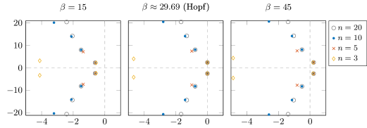
Figure 2: Pseudospectral approximation to (2.1) with $\tau=1$ and $h(x)=e^{-x}$: roots of the characteristic equation at the positive equilibrium for $\mu=3$ and different values of $\beta$ as indicated at the top (corresponding to the three black crosses in Figure 1). The eigenvalues are approximated with MatCont.

6 Hopf bifurcation in the pseudospectral limit

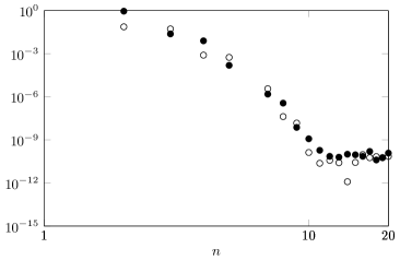
Figure 3: Equation (2.1) with $\tau=1$ and $h(x)=e^{-x}$: log-log plot of the error in the detection of Hopf point (bullets) and in the approximation of the imaginary part of the rightmost roots of the characteristic equation at Hopf (circles), at $\mu=3$. The errors are calculated by requiring a tolerance of $10^{-9}$ in MatCont computations, and by calculating the absolute value of the difference between the MatCont output and the analytic values. Note the exponential decay until the accuracy $10^{-10}$ is reached.

In the following, we denote a generic Hopf bifurcation by the triple $(\alpha,\omega,a_{2})$, where $\alpha$ is the bifurcation point, $i\omega$ the root of the characteristic equation on the imaginary axis and $a_{2}$ the direction coefficient. Here we use the word generic to indicate the three standard conditions ($1.$ simple root of the characteristic equation; $2.$ transversal crossing; $3.$ non-resonance) and we do not require that the direction coefficient is non-zero. To show that the Hopf bifurcation in the pseudospectral approximation is a faithful representation of the Hopf bifurcation in the DDE, we have to answer the following questions:

Question 1.

If the DDE has a generic Hopf bifurcation $(\alpha_{0},\omega_{0},a_{20})$, do the pseudospectral ODE have Hopf bifurcations $(\alpha_{n},\omega_{n},a_{2n})$ with $\lim_{n\to\infty}(\alpha_{n},\omega_{n},a_{2n})=(\alpha_{0},\omega_{0},a_{20})$?

Question 2.

Vice versa, if the pseudospectral ODE have generic Hopf bifurcations $(\alpha_{n},\omega_{n},a_{2n})$ with

$$\lim_{n\to\infty}(\alpha_{n},\omega_{n},a_{2n})=(\alpha_{0},\omega_{0},a_{20}),$$

does the DDE have a Hopf bifurcation $(\alpha_{0},\omega_{0},a_{20})$?

Answering these questions involves checking the following conditions:

1. At the bifurcation point, there is a simple root of the characteristic equation on the imaginary axis.

2. This root of the characteristic equation on the imaginary axis crosses the axis transversely if we vary the parameter.

3. At the bifurcation point, there are no roots of the characteristic equation in resonance with the root on the imaginary axis.

4. Convergence of the direction coefficients.

We first answer Question 1. To check conditions $1$ and $2$, we use the following lemma, which can be viewed as a version of the Implicit Function Theorem with a (discrete) parameter living in $\mathbb{N}$. It is inspired by [29, Theorem A.1] where the parameter belongs to a general metric space.

Lemma 6.1.

Let $h_{0}:\mathbb{R}^{d}\to\mathbb{R}^{d}$ and $h_{n}:\mathbb{R}^{d}\to\mathbb{R}^{d},\ n\in\mathbb{N},$ be $C^{1}$ functions with

$$h_{0}(x)=\lim_{n\to\infty}h_{n}(x)\quad\mbox{and}\quad Dh_{0}(x)=\lim_{n\to\infty}Dh_{n}(x)$$ (6.1)

uniformly for $x$ in compact subsets of $\mathbb{R}^{d}$. Given a compact subset $U\subset\mathbb{R}^{d}$, let $(\rho_{n})_{n\in\mathbb{N}}=(\rho_{n}(U))_{n\in\mathbb{N}}$ be a sequence such that

$$\left\lVert h_{n}(x)-h_{0}(x)\right\rVert\leq\rho_{n}\quad\mbox{for all }n\in\mathbb{N}\mbox{ and }x\in U.$$ (6.2)

Assume that there exists $x_{0}\in\mathbb{R}^{d}$ such that $h_{0}(x_{0})=0$ and $Dh_{0}(x_{0})$ is invertible. Then there exists a sequence $(x_{n})_{n\in\mathbb{N}}$ such that for $n$ large enough, $h_{n}(x_{n})=0$ and $Dh_{n}(x_{n})$ is invertible. Moreover, there exists a constant $C>0$ such that

$$\left\lVert x_{n}-x_{0}\right\rVert\leq C\rho_{n},\quad n\in\mathbb{N}\quad\mbox{ with }\rho_{n}=\rho_{n}(U).$$

Proof.

Define the functions

$$f_{0}(x)=x-Dh_{0}(x_{0})^{-1}h_{0}(x),\quad f_{n}(x)=x-Dh_{0}(x_{0})^{-1}h_{n}(x)$$

so that zero’s of $h_{n},h_{0}$ correspond to fixed points of $f_{n},f_{0}$, respectively. Note that $Df_{0}(x_{0})=0$ and

$$\lim_{n\to\infty}Df_{n}(x)=Df_{0}(x)\qquad\mbox{uniformly for }x\mbox{ in compact subsets}.$$

Therefore we can find a $\rho>0$ and a $0<q<1$ such that $\|Df_{n}(x)\|<q$ for all $n\in\mathbb{N},\ x\in B(x_{0},\rho)$. From the Mean Value Theorem we obtain that, for all $n\in\mathbb{N}$, $f_{n}:B(x_{0},\rho)\to\mathbb{R}^{d}$ is Lipschitz with Lipschitz constant $q$. From the Contraction Mapping Principle, it follows that for all $n\in\mathbb{N}$, $f_{n}$ has a unique fixed point $x_{n}$ in $B(x_{0},\rho)$. Moreover, if we let $U$ be a neighbourhood of $x_{0}$ and $(\rho_{n})_{n\in\mathbb{N}}$ be as in (6.2), then

$$\left\lVert x_{n}-x_{0}\right\rVert \leq\left\lVert f_{n}(x_{n})-f_{n}(x_{0})\right\rVert+\left\lVert f_{n}(x_{0})-f_{0}(x_{0})\right\rVert$$

$$<q\left\lVert x_{n}-x_{0}\right\rVert+\left\lVert Dh_{0}(x_{0})^{-1}\right\rVert\rho_{n}.$$

This yields the estimate

$$\left\lVert x_{n}-x_{0}\right\rVert\leq\frac{\rho_{n}}{1-q}\|Dh_{0}(x_{0})^{-1}\|.$$

Moreover, since $\lim_{n\to\infty}Dh_{n}(x_{n})=Dh_{0}(x_{0})$ and $Dh(x_{0})$ is invertible, $Dh_{n}(x_{n})$ is invertible for $n$ large enough. ∎

Proposition 6.2.

Consider system (3.3) and suppose that Hypothesis 2 is satisfied. Moreover, suppose that there exist $\alpha_{0}\in\mathbb{R}$ and $\omega_{0}>0$ such that

1. $i\omega_{0}$ is a simple root of $\Delta_{0}(\lambda,\alpha_{0})=0$;

2. The branch of roots of $\Delta_{0}(\lambda,\alpha)=0$ through $i\omega_{0}$ at $\alpha=\alpha_{0}$ intersects the imaginary axis transversally, i.e.,

   $$\mbox{Re}\,\left(D_{1}\Delta_{0}(i\omega_{0},\alpha_{0})^{-1}D_{2}\Delta_{0}(i\omega_{0},\alpha_{0})\right)\neq 0.$$ (6.3)

Then, for $n$ large enough, there exist $\alpha_{n}\in\mathbb{R}$, $\omega_{n}>0$ such that

1. $i\omega_{n}$ is a simple root of $\Delta_{n}(\lambda,\alpha_{n})=0$;

2. the branch of roots of $\Delta_{n}(\lambda,\alpha)=0$ through $i\omega_{n}$ at $\alpha=\alpha_{n}$ intersects the imaginary axis transversally, i.e.

   $$\mbox{Re}\,\bigl{(}D_{1}\Delta_{n}(i\omega_{n},\alpha_{n})^{-1}D_{2}\Delta_{n}(i\omega_{n},\alpha_{n})\bigr{)}\neq 0.$$ (6.4)

Moreover, there exists a $C>0$ such that

$$\left\lVert(\alpha_{n},\omega_{n})-(\alpha_{0},\omega_{0})\right\rVert\leq\frac{1}{\sqrt{n}}\left(\frac{C}{n}\right)^{n},\quad\mbox{for }n\in\mathbb{N}\mbox{ large enough}.$$ (6.5)

Proof.

Define the functions $h_{n},h_{0}:\mathbb{R}^{2}\to\mathbb{R}^{2}$ as

$$h_{n}(\omega,\alpha)=\begin{pmatrix}\mbox{Re}\,\Delta_{n}(i\omega,\alpha)\\ \mbox{Im}\,\Delta_{n}(i\omega,\alpha)\end{pmatrix},\qquad h_{0}(\omega,\alpha)=\begin{pmatrix}\mbox{Re}\,\Delta_{0}(i\omega,\alpha)\\ \mbox{Im}\,\Delta_{0}(i\omega,\alpha)\end{pmatrix}.$$

Then $h_{0}(\omega_{0},\alpha_{0})=0$ and (6.1) is satisfied by Corollary 5.2 and Corollary 5.4. In order to apply Lemma 6.1, we only have to check that $Dh_{0}(\omega_{0},\alpha_{0})$ is invertible.

For $\sigma,\omega\in\mathbb{R}$, write

$$\Delta_{0}(\sigma+i\omega,\alpha_{0})=f_{1}(\sigma,\omega)+if_{2}(\sigma,\omega)$$

with $f_{1},f_{2}\in\mathbb{R}$. With this notation $Dh_{0}(\omega_{0},\alpha_{0})$ becomes

$$Dh_{0}(\omega_{0},\alpha_{0})=\begin{pmatrix}D_{2}f_{1}(0,\omega_{0})&\mbox{Re}\,D_{2}\Delta_{0}(i\omega_{0},\alpha_{0})\\ D_{2}f_{2}(0,\omega_{0})&\mbox{Im}\,D_{2}\Delta_{0}(i\omega_{0},\alpha_{0})\end{pmatrix}.$$

The Cauchy-Riemann equations read

$$D_{2}f_{1}(\sigma,\omega)=-D_{1}f_{2}(\sigma,\omega),\qquad D_{2}f_{2}(\sigma,\omega)=D_{1}f_{1}(\sigma,\omega)$$

and hence

$$Dh_{0}(\omega_{0},\alpha_{0})=\begin{pmatrix}-D_{1}f_{2}(0,\omega_{0})&\mbox{Re}\,D_{2}\Delta_{0}(i\omega_{0},\alpha_{0})\\ D_{1}f_{1}(0,\omega_{0})&\mbox{Im}\,D_{2}\Delta_{0}(i\omega_{0},\alpha_{0})\end{pmatrix}.$$ (6.6)

But now note that if we compute $D_{1}\Delta_{0}(i\omega_{0},\alpha_{0})$, we may as well compute the difference quotient by taking the limit over the real axis, so

$$\mbox{Re}\,D_{1}\Delta_{0}(i\omega_{0},\alpha_{0})=D_{1}f_{1}(0,\omega_{0}),\qquad\mbox{Im}\,D_{1}\Delta_{0}(i\omega_{0},\alpha_{0})=D_{1}f_{2}(0,\omega_{0})$$

and (6.6) becomes

$$Dh_{0}(\omega_{0},\alpha_{0})=\begin{pmatrix}-\mbox{Im}\,D_{1}\Delta_{0}(i\omega_{0},\alpha_{0})&\mbox{Re}\,D_{2}\Delta_{0}(i\omega_{0},\alpha_{0})\\ \mbox{Re}\,D_{1}\Delta_{0}(i\omega_{0},\alpha_{0})&\mbox{Im}\,D_{2}\Delta_{0}(i\omega_{0},\alpha_{0})\end{pmatrix}.$$

The invertibility of the matrix $Dh_{0}(\omega_{0},\alpha_{0})$ is equivalent to the condition (6.3). So we can apply Lemma 6.1 to find a sequences $(i\omega_{n})_{n\in\mathbb{N}},(\alpha_{n})_{n\in\mathbb{N}}$ with $\Delta_{n}(i\omega_{n},\alpha_{n})=0$ and with the error estimate (6.5). Moreover, a similar argument as before gives that the invertibility of $Dh_{n}(\omega_{n},\alpha_{n})$ is equivalent to the condition (6.4). ∎

For equation (2.1), the statements of Proposition 6.2 are illustrated in Figure 2–3. In Figure 2, the roots of the characteristic equation of the pseudospectral approximation of (2.1) are plotted for different values of the parameter $\beta$. Figure 3 shows the error in the detection of the Hopf point and the imaginary part of the root of the characteristic equation for the pseudospectral approximation. We see that the desired tolerance level is obtained for relatively low values of the discretisation index ($n\approx 10$).

Next we look at the non-resonance condition. Suppose that $\Delta_{0}(i\omega_{0},\alpha_{0})=0$ but $\Delta_{0}(ki\omega_{0},\alpha_{0})\neq 0$ for all $k=0,2,\ldots$. Corollary 5.2 gives that for fixed $k$, there exists a $N=N(k)$ such that $\Delta_{n}(ki\omega_{n},\alpha_{n})\neq 0$ for $n\geq N(k)$. However, this does not imply that we can choose this $N$ to be uniform in $k$, i.e., that we can find a $N$ such that

$$\Delta_{n}(ki\omega_{n},\alpha_{n})\neq 0\quad\mbox{for all }n\geq N\mbox{ and all }\ k=0,2,3,\ldots.$$ (6.7)

So Corollary 5.2 does not exclude that for every $n\in\mathbb{N}$ large enough there exists a $k(n)$ such that $\Delta_{n}(k(n)i\omega_{n},\alpha_{n})=0$. This is clearly a non-generic situation, but in order to answer the third condition listed below Question 2, we have to exclude it explicitly. See also Section 8.

Concerning the convergence of the direction coefficient we find:

Lemma 6.3.

Consider system (3.3) and suppose that the hypotheses of Theorem 3.2 are satisfied. Let $(\alpha_{n},\omega_{n})$ be as in Proposition 6.2. Then $\lim_{n\to\infty}a_{2n}=a_{20}$. Moreover, if the nonlinearity $g:X\times\mathbb{R}\to X$ is $C^{4}$, then there exists a $C>0$ such that

$$\left|a_{2n}-a_{20}\right|\leq\frac{1}{\sqrt{n}}\left(\frac{C}{n}\right)^{n}\qquad\mbox{for }n\in\mathbb{N}\mbox{ large enough}.$$

Proof.

Throughout the proof, we use the symbol $C$ to denote a generic constant whose actual value may differ from line to line. For instance, an upper bound $C_{1}C^{n}$, with $C_{1}>1$ , is replaced by the upperbound $C^{n}$ , with the second $C$ slightly larger than the first $C$.

We first prove that $\lim_{n\to\infty}c_{n}=c_{0}$, with $c_{n}$ defined as in (4.27) and $c_{0}$ defined as in (3.6). Given a compact neighbourhood $U$ of $i\omega_{0}$, Lemma 5.1 gives a constant $C>0$ such that

$$\left\lVert\varepsilon_{\lambda}-P_{0}(1,(D-\lambda I)^{-1}D\textbf{1})\right\rVert\leq\frac{1}{\sqrt{n}}\left(\frac{C}{n}\right)^{n}$$ (6.8)

for all $\lambda\in U$. By Proposition 6.2, there exists a $C>0$ such that $\left\lVert(i\omega_{n},\alpha_{n})-(i\omega_{0},\alpha_{0})\right\rVert<\frac{1}{\sqrt{n}}\left(\frac{C}{n}\right)^{n}$. Since the map $\lambda\mapsto\varepsilon_{\lambda}(\theta)$ is locally Lipschitz continuous, uniformly for $\theta\in[-1,0]$, we can find a $C>0$ such that

$$\left\lVert\varepsilon_{i\omega_{0}}-\varepsilon_{i\omega_{n}}\right\rVert\leq\frac{1}{\sqrt{n}}\left(\frac{C}{n}\right)^{n}$$ (6.9)

holds. Using (6.8) and (6.9) we obtain the estimate

$$\left\lVert\varepsilon_{i\omega_{0}}-P_{0}(1,(D-i\omega_{n}I)^{-1}D\textbf{1})\right\rVert \leq\left\lVert\varepsilon_{i\omega_{0}}-\varepsilon_{i\omega_{n}}\right\rVert+\left\lVert\varepsilon_{i\omega_{n}}-P_{0}(1,(D-i\omega_{n}I)^{-1}D\textbf{1})\right\rVert$$ (6.10)

$$\leq\frac{1}{\sqrt{n}}\left(\frac{C}{n}\right)^{n}.$$

We compare the first term of $c_{n}$ defined in (4.27) with the first term of $c_{0}$ defined in (3.6). Writing $p=(1,(D-i\omega_{n})^{-1}D\textbf{1})$ and $\phi=\varepsilon_{i\omega_{0}}$, we estimate

$$\left\lVert D_{1}^{3}g(0,\alpha_{n})(P_{0}p,P_{0}p,P_{0}\overline{p})-D_{1}^{3}g(0,\alpha_{0})(\phi,\phi,\overline{\phi})\right\rVert\leq \left\lVert D_{1}^{3}g(0,\alpha_{n})(\phi,\phi,\overline{\phi})-D_{1}^{3}g(0,\alpha_{0})(\phi,\phi,\overline{\phi})\right\rVert$$ (6.11)

$$+\left\lVert D_{1}^{3}g(0,\alpha_{n})(\phi,\phi,\overline{\phi})-D_{1}^{3}g(0,\alpha_{n})(P_{0}p,P_{0}p,P_{0}\overline{p})\right\rVert$$

Since the map $\alpha\mapsto D_{1}^{3}g(0,\alpha)$ is continuous and $\alpha_{n}\to\alpha_{0}$ as $n\to\infty$, we obtain that

$$\left\lVert D_{1}^{3}g(0,\alpha_{n})(\phi,\phi,\overline{\phi})-D_{1}^{3}g(0,\alpha_{0})(\phi,\phi,\overline{\phi})\right\rVert\to 0$$

as $n\to\infty$. If $g$ is $C^{4}$, then the map $\alpha\mapsto D_{1}^{3}g(0,\alpha)(\phi,\phi,\overline{\phi})$ is locally Lipschitz and we obtain

$$\left\lVert D_{1}^{3}g(0,\alpha_{n})(\phi,\phi,\overline{\phi})-D_{1}^{3}g(0,\alpha_{0})(\phi,\phi,\overline{\phi})\right\rVert \leq C\left|\alpha_{n}-\alpha_{0}\right|$$ (6.12)

$$\leq\frac{1}{\sqrt{n}}\left(\frac{C}{n}\right)^{n}.$$

Since the map $(u,v,w)\mapsto D_{1}^{3}g(0,\alpha_{n})(u,v,w)$ is linear in every argument, we can rewrite

$$D_{1}^{3}g(0,\alpha_{n})(\phi,\phi,\overline{\phi})-D_{1}^{3}g(0,\alpha_{n})(P_{0}p,P_{0}p,P_{0}\overline{p})$$

$$=D_{1}^{3}g(0,\alpha_{n})(\phi-P_{0}p,\phi,\overline{\phi})+D_{1}^{3}g(0,\alpha_{n})(P_{0}p,\phi-P_{0}p,\overline{\phi})+D_{1}^{3}g(0,\alpha_{n})(P_{0}p,P_{0}p,\overline{\phi}-P_{0}\overline{p}).$$

Combining this with (6.10), we obtain the estimate

$$\left\lVert D_{1}^{3}g(0,\alpha_{n})(\phi,\phi,\overline{\phi})-D_{1}^{3}g(0,\alpha_{n})(P_{0}p,P_{0}p,P_{0}\overline{p})\right\rVert\leq\frac{1}{\sqrt{n}}\left(\frac{C}{n}\right)^{n}.$$ (6.13)

So from (6.11), (6.12) and (6.13) we conclude that

$$\lim_{n\to\infty}D_{1}^{3}g(0,\alpha_{n})(P_{0}p,P_{0}p,P_{0}\overline{p})=D_{1}^{3}g(0,\alpha_{0})(\phi,\phi,\overline{\phi})$$

and if $g$ is $C^{4}$, then

$$\left\lVert D_{1}^{3}g(0,\alpha_{n})(P_{0}p,P_{0}p,P_{0}\overline{p})-D_{1}^{3}g(0,\alpha_{0})(\phi,\phi,\overline{\phi})\right\rVert\leq\frac{1}{\sqrt{n}}\left(\frac{C}{n}\right)^{n}.$$ (6.14)

Now suppose that $(x_{n})_{n\in\mathbb{N}}\subseteq\mathbb{C},\ (y_{n})_{n\in\mathbb{N}}\subseteq\mathbb{C}\backslash\{0\}$ are sequences with $\lim_{n\to\infty}x_{n}=x_{0},\ \lim_{n\to\infty}y_{n}=y_{0}\neq 0$. Then we find for their fraction

$$\left|\frac{x_{n}}{y_{n}}-\frac{x_{0}}{y_{0}}\right|=\left|\frac{x_{n}y_{0}-x_{0}y_{n}}{y_{n}y_{0}}\right|\leq\left|\frac{(x_{n}-x_{0})y_{0}}{y_{n}y_{0}}\right|+\left|\frac{x_{0}(y_{n}-y_{0})}{y_{n}y_{0}}\right|\leq C\left(\left|x_{n}-x_{0}\right|+\left|y_{n}-y_{0}\right|\right).$$ (6.15)

By Corollary 5.4, there exists a $C>0$ such that

$$\left|D_{1}\Delta_{n}(i\omega_{n},\alpha_{n})-D_{1}\Delta_{0}(i\omega_{0},\alpha_{0})\right|\leq\frac{1}{\sqrt{n}}\left(\frac{C}{n}\right)^{n}.$$

So if we apply (6.15) with $x_{n}=D_{1}^{3}g(0,\alpha_{n})(P_{0}p,P_{0}p,P_{0}\overline{p})$ and $y_{n}=D_{1}\Delta_{n}(i\omega_{n},\alpha_{n})$, we see that

$$\left\lVert D_{1}\Delta_{n}(i\omega_{n},\alpha_{n})^{-1}D_{1}^{3}g(0,\alpha_{n})(P_{0}p,P_{0}p,P_{0}\overline{p})-D_{1}\Delta_{0}(i\omega_{0},\alpha_{0})^{-1}D_{1}^{3}g(0,\alpha_{0})(\phi,\phi,\overline{\phi})\right\rVert\to 0\mbox{ as }n\to\infty$$

and if $g$ is $C^{4}$, then

$$\left\lVert D_{1}\Delta_{n}(i\omega_{n},\alpha_{n})^{-1}D_{1}^{3}g(0,\alpha_{n})(P_{0}p,P_{0}p,P_{0}\overline{p})-D_{1}\Delta_{0}(i\omega_{0},\alpha_{0})^{-1}D_{1}^{3}g(0,\alpha_{0})(\phi,\phi,\overline{\phi})\right\rVert\leq\frac{1}{\sqrt{n}}\left(\frac{C}{n}\right)^{n}.$$

Applying similar arguments to the second and third term of $c_{n}$, we find that $\lim_{n\to\infty}c_{n}=c_{0}$; if $g$ is $C^{4}$, we obtain the error estimate

$$\left|c_{n}-c_{0}\right|\leq\frac{1}{\sqrt{n}}\left(\frac{C}{n}\right)^{n}.$$

To analyse the convergence of the direction coefficient $a_{2n}$, we apply (6.15) with $x_{n}=\mbox{Re}\,c_{n}$ and $y_{n}=\mbox{Re}\,\left(D_{1}\Delta_{n}(i\omega_{n},\alpha_{n})^{-1}D_{2}\Delta_{n}(i\omega_{n},\alpha_{n})\right)$. We conclude that

$$\left|a_{2n}-a_{20}\right|\to 0\quad\mbox{as }n\to\infty$$

and if $g$ is $C^{4}$, then

$$\left|a_{2n}-a_{20}\right|\leq\frac{1}{\sqrt{n}}\left(\frac{C}{n}\right)^{n}$$

which proves the claim. ∎

Summarising, we find the following answer to Question 1:

Proposition 6.4.

Consider system (3.3) and suppose that the hypotheses of Theorem 3.2 are satisfied. Moreover, with $\alpha_{n},\omega_{n}$ as in Proposition 6.2, assume that

$$\mbox{for }n\in\mathbb{N}\mbox{ large enough, }\qquad\Delta_{n}(ki\omega_{n},\alpha_{n})\neq 0\qquad\mbox{ for }k=0,2,3,\ldots$$ (6.16)

Then the hypotheses of Theorem 4.1 are satisfied and $\lim_{n\to\infty}a_{2n}=a_{20}$. Moreover, if the nonlinearity $g:X\times\mathbb{R}\to X$ is $C^{4}$, then there exists a $C>0$ such that

$$\left|a_{2n}-a_{20}\right|\leq\frac{1}{\sqrt{n}}\left(\frac{C}{n}\right)^{n}\qquad\mbox{for }n\in\mathbb{N}\mbox{ large enough}.$$

We now consider Question 2. Suppose that we have sequences $(\alpha_{n})_{n\in\mathbb{N}}$, $(\omega_{n})_{n\in\mathbb{N}}$ with $\lim_{n\to\infty}\alpha_{n}=\alpha\in\mathbb{R},\ \lim_{n\to\infty}\omega_{n}=\omega_{0}\neq 0$. Suppose that $i\omega_{n}$ is a simple root of $\Delta_{n}(\lambda,\alpha_{n})=0$ and such that this root crosses the axis transversely if we vary $\alpha$. Then $\Delta_{0}(i\omega_{0},\alpha_{0})=0$ but we have to make additional assumptions to make sure that this root is simple and it crosses the axis transversely if we vary $\alpha$. Similarly, if for $n\in\mathbb{N}$ large enough, it holds that $\Delta_{n}(ki\omega_{n},\alpha_{n})\neq 0$ for $k=0,2,3,\ldots$, we have to make additional assumptions to ensure that $\Delta_{0}(ki\omega_{0},\alpha_{0})\neq 0$ for $k=0,2,3\ldots$.

Proposition 6.5.

Consider system (3.3) and suppose that there exists a $N_{0}\in\mathbb{N}$ such that for $n\in\mathbb{N},\ n\geq N_{0}$ the hypotheses of Theorem 4.1 are satisfied with $\lim_{n\to\infty}\alpha_{n}=\alpha_{0},\ {\color[rgb]{0,0,0}\lim_{n\to\infty}\omega_{n}=\omega_{0}\neq 0}$ and $\lim_{n\to\infty}a_{2n}=a_{20}^{\prime}$. Moreover, suppose that

1. The sequence $(D_{1}\Delta_{n}(i\omega_{n},\alpha_{n}))_{n\geq N_{0}}$ is uniformly bounded away from zero;

2. The sequence $\left(\mbox{Re}\,\left(D_{1}\Delta_{n}(i\omega_{n},\alpha_{n})^{-1}D_{2}\Delta_{n}(i\omega_{n},\alpha_{n})\right)\right)_{n\geq N_{0}}$ is uniformly bounded away from zero;

3. For each $k=0,2,3\ldots$, the sequence $(\Delta_{n}(ki\omega_{n},\alpha_{n}))_{n\geq N_{0}}$ is uniformly bounded away from zero.

Then the Hypotheses of Theorem 3.2 are satisfied and the direction coefficient is given by $a_{20}^{\prime}$, i.e. $a_{20}=a_{20}^{\prime}$.

Proof.

Taking the limit in $\Delta_{n}(i\omega_{n},\alpha_{n})=0$ gives that $\Delta_{0}(i\omega_{0},\alpha_{0})=0$. The conditions (1), (2) and (3) ensure that $D_{1}\Delta_{0}(i\omega_{0},\alpha_{0})\neq 0$, $\mbox{Re}\,\left((D_{1}\Delta(i\omega_{0},\alpha_{0}))^{-1}D_{2}\Delta(i\omega_{0},\alpha_{0})\right)\neq 0$ and $\Delta_{0}(ki\omega_{0},\alpha_{0})\neq 0$ for $k=0,2,3,\ldots$. Moreover, as in the proof of Lemma 6.3 we find that $\lim_{n\to\infty}a_{2n}=a_{20}$, which implies that $a_{20}=a_{20}^{\prime}$. ∎

7 Systems

We formulate the relevant definitions and results for systems of DDE.

Let $d\in\mathbb{N}$ and consider the system

$$x^{\prime}(t)=L(\alpha)x_{t}+g(x_{t},\alpha),\quad t\geq 0$$ (7.1)

with state space $X=C\left([-1,0],\mathbb{R}^{d}\right)$, $\alpha\in\mathbb{R}$ a parameter, $L(\alpha):X\to\mathbb{R}^{d}$ a bounded linear operator and $g:X\times\mathbb{R}\to\mathbb{R}^{d}$. We summarise the relevant assumptions on $L$ and $g$ in the following hypothesis:

Hypothesis 3.

1. $g:X\times\mathbb{R}\to\mathbb{R}^{d}$ and $\alpha\to L(\alpha)$ are $C^{k}$ smooth for some $k\geq 3$;

2. $g(0,\alpha)=0$ and $D_{1}g(0,\alpha)=0$ for all $\alpha\in\mathbb{R}$.

Under this hypothesis, (7.1) has an equilibrium $x=0$ for all $\alpha\in\mathbb{R}$. The linearisation of (7.1) has a solution of the form $t\mapsto e^{\lambda t}c,\ c\in\mathbb{C}^{d}$ if and only if $\lambda$ is a root of the characteristic equation

$$\det\Delta_{0}(\lambda,\alpha)=0$$

where the operator $\Delta_{0}(\lambda,\alpha):\mathbb{C}^{d}\to\mathbb{C}^{d}$ is defined as

$$\Delta_{0}(\lambda,\alpha)=\lambda I_{d}-L(\alpha)\varepsilon_{\lambda}$$ (7.2)

with $I_{d}:\mathbb{C}^{d}\to\mathbb{C}^{d}$ is the identity operator and $\varepsilon_{\lambda}$ defined as in (3.5). In (7.2), $L(\alpha)\varepsilon_{\lambda}$ maps $\mathbb{C}^{d}$ to $\mathbb{C}^{d}$ in the following way: given $v\in\mathbb{C}^{d}$, the function $(\varepsilon_{\lambda}v)(\theta)=\varepsilon_{\lambda}(\theta)v$ is an element of $C\left([-1,0],\mathbb{C}^{d}\right)$; then $L(\alpha)\left(\varepsilon_{\lambda}v\right)$ is a vector in $\mathbb{C}^{d}$.

If $i\omega_{0}$ is a simple root of $\det\Delta_{0}(\lambda,\alpha_{0})=0$, then $\Delta_{0}(i\omega_{0},\alpha_{0})$ has a one-dimensional kernel. Moreover, if $p,q\in\mathbb{C}^{d}\backslash\{0\}$ are such that $\Delta_{0}(i\omega_{0},\alpha_{0})p=0,\ \Delta_{0}(i\omega_{0},\alpha_{0})^{T}q=0$, then $q\cdot D_{1}\Delta_{0}(i\omega_{0},\alpha_{0})p\neq 0$, see [14, Exercise IV.3.12]. In particular, we can (and will) scale $p,q$ such that $q\cdot D_{1}\Delta_{0}(i\omega_{0},\alpha_{0})p=1$.

Theorem 7.1 (Hopf bifurcation theorem for systems of DDE).

Consider system (7.1) and suppose that Hypothesis 3 is satisfied. Moreover, suppose that there exist $\alpha_{0}\in\mathbb{R}$ and $\omega_{0}>0$ such that

1. $i\omega_{0}$ is a simple root of $\det\Delta_{0}(\lambda,\alpha_{0})=0$;

2. The branch of roots of $\det\Delta_{0}(\lambda,\alpha)=0$ through $i\omega_{0}$ at $\alpha=\alpha_{0}$ intersects the imaginary axis transversally, i.e., the real part of the derivative of the roots along the branch is non-zero. If we denote by $p,q\in\mathbb{C}^{d}\backslash\{0\}$ the vectors such that $\Delta_{0}(i\omega_{0},\alpha_{0})p=0,\ \Delta_{0}(i\omega_{0},\alpha_{0})^{T}q=0$ and $q\cdot D_{1}\Delta_{0}(i\omega_{0},\alpha_{0})p=1$, then this condition amounts to

   $$\mbox{Re}\,\left(q\cdot D_{2}\Delta_{0}(i\omega_{0},\alpha_{0})p\right)\neq 0;$$

3. $ki\omega_{0}$ is not a root of $\det\Delta_{0}(\lambda,\alpha_{0})$ for $k=0,2,3,\ldots$

Then a Hopf bifurcation occurs for $\alpha=\alpha_{0}$. This means that there exist $C^{k-1}$-functions $\epsilon\mapsto\alpha^{\ast}(\epsilon)$, $\epsilon\mapsto\omega^{\ast}(\epsilon)$ taking values in $\mathbb{R}$ and $\epsilon\mapsto x^{\ast}(\epsilon)\in C_{b}\left(\mathbb{R},\mathbb{R}^{d}\right)$, all defined for $\epsilon$ sufficiently small, such that for $\alpha=\alpha^{\ast}(\epsilon),\ x^{\ast}(\epsilon)$ is a periodic solution of (7.1) with period $2\pi/\omega^{\ast}(\epsilon)$. Moreover, $\alpha^{\ast},\omega^{\ast}$ are even functions, $\alpha^{\ast}(0)=\alpha_{0},\ \omega^{\ast}(0)=\omega_{0}$ and if $x$ is any small periodic solution of(7.1) for $\alpha$ close to $\alpha_{0}$ and minimal period close to $2\pi/\omega_{0}$, then $x(t)=x^{\ast}(\epsilon)(t+\theta^{\ast})$ and $\alpha=\alpha^{\ast}(\epsilon)$ for some $\epsilon$ and some $\theta\in[0,2\pi/\omega^{\ast}(\epsilon))$.

Moreover, $\alpha^{\ast}$ has the expansion $\alpha^{\ast}(\epsilon)=\alpha_{0}+a_{20}\epsilon^{2}+o(\epsilon^{2})$, with $a_{20}$ given by

$$a_{20}=\frac{\mbox{Re}\,c}{\mbox{Re}\,\left(q\cdot D_{2}\Delta_{0}(i\omega_{0},\alpha_{0})p\right)}$$

where

$$c= \frac{1}{2}q\cdot D_{1}^{3}g(0,\alpha_{0})(\phi,\phi,\overline{\phi})$$ (7.3)

$$\qquad+q\cdot D_{1}^{2}g(0,\alpha_{0})\bigl{(}\varepsilon_{0}\Delta_{0}(0,\alpha_{0})^{-1}D_{1}^{2}g(0,\alpha_{0})(\phi,\overline{\phi}),\phi\bigr{)}$$

$$\qquad+\frac{1}{2}q\cdot D_{1}^{2}g(0,\alpha_{0})\bigl{(}\varepsilon_{2i\omega_{0}}\Delta_{0}(2i\omega_{0},\alpha_{0})^{-1}D_{1}^{2}g(0,\alpha_{0})(\phi,\phi),\overline{\phi}\bigr{)}\bigr{)}$$

with $\phi:=\varepsilon_{i\omega_{0}}p$.

To write down the pseudospectral approximation to (7.1), let for $j=0,\ldots,n$

$$y_{j}(t)\in\mathbb{R}^{d}$$

and denote the components of this vector as

$$y_{j}(t)(k),\qquad k=1,\ldots d.$$

We define the interpolation operators $P:\mathbb{R}^{nd}\to X,\ P_{0}:\mathbb{R}^{d}\times\mathbb{R}^{nd}\to X$ componentwise as

$$\left(Py\right)_{k}(\theta) :=\sum_{j=1}^{n}\ell_{j}(\theta)y_{j}(k)$$

$$\left(P_{0}(y_{0},y)\right)_{k} :=\ell_{0}(\theta)y_{0}(k)+\left(Py\right)_{k}(\theta)$$

where $\ell_{j},\ j=0,1,\ldots,n$ are defined by (4.1). We approximate

$$x_{k}(t+\theta)\sim\sum_{j=0}^{n}\ell_{j}(\theta)y_{j}(t)(k),\qquad k=1,\ldots d$$

and by collocation on the meshpoints $\theta_{1},\ldots,\theta_{n}$ we obtain

$$y_{i}^{\prime}(t)(k)=\sum_{j=1}^{n}D_{ij}y_{j}(t)(k)-y_{0}(t)(k)\left[D\textbf{1}\right]_{i},\qquad i=1,\ldots,n$$ (7.4)

with $D$ as in (4.5). To approximate the rule for extension, we supplement (7.4) with

$$y_{0}^{\prime}(t)=L(\alpha)P_{0}(y_{0},y)+g(P_{0}(y_{0},y),\alpha).$$ (7.5)

Suppressing the index $i$ in the notation we write (7.4) as

$$y^{\prime}(t)(k)=Dy(t)(k)-y_{0}(t)(k)D\textbf{1},\qquad k=1,\ldots d$$ (7.6)

and next, by suppressing $k$, abbreviate to

$$y^{\prime}=Dy-y_{0}D\textbf{1}$$

where this expression is to be understood $d$-componentwise as in (7.6). With this notation, the pseudospectral approximation to (7.1) becomes

$$y_{0}^{\prime}(t) =L(\alpha)P_{0}(y_{0},y)+g(P_{0}(y_{0},y),\alpha),$$ (7.7)

$$y^{\prime}(t) =Dy(t)-y_{0}(t)D\textbf{1}.$$

The linearisation of (7.7) around $x=0$ has a solution of the form $\varepsilon_{\lambda}(\zeta_{0},\zeta)$ if and only if

$$\lambda\zeta_{0} =L(\alpha)\ell_{0}\zeta_{0}+L(\alpha)P\zeta$$ (7.8a)

$$\lambda\zeta =D\zeta-\zeta_{0}D\textbf{1}$$ (7.8b)

with $\zeta_{j}\in\mathbb{C}^{d}$ for $j=0,\ldots,n$. The $d$-componentwise nature of (7.8b) allows us to write

$$\zeta_{j}(k)=\zeta_{0}(k)\left[(D-\lambda I)^{-1}D\textbf{1}\right]_{j},\qquad j=0,\ldots,n,\quad k=1,\ldots,d,$$

which we abbreviate in the compact notation

$$\zeta=\zeta_{0}(D-\lambda I)^{-1}D\textbf{1}.$$ (7.9)

Substituting (7.9) into (7.8a) gives that (7.8a)–(7.8b) has a nontrivial solution if and only if

$$\det\Delta_{n}(\lambda,\alpha)\neq 0$$

with

$$\Delta_{n}(\lambda,\alpha)=\lambda I_{d}-L(\alpha)\left(\ell_{0}I_{d}+P(D-\lambda I)^{-1}D\textbf{1}\right).$$

If $\det\Delta_{n}(\lambda,\alpha)=0$, then (7.8a)–(7.8b) has a non-trivial solution of the form $(p_{\ast},p_{\ast}(D-\lambda I)^{-1}D\textbf{1})$, where $p_{\ast}\neq 0$ satisfies $\Delta_{n}(\lambda,\alpha)p_{\ast}=0$.

Applying Theorem 3.1 to system (7.7) we obtain:

Theorem 7.2 (Hopf bifurcation in pseudospectral ODE).

Consider the system (7.1) and suppose that Hypothesis 3 is satisfied. If there exist $\alpha_{n}\in\mathbb{R}$ and $\omega_{n}>0$ such that

1. $i\omega_{n}$ is a simple root of $\det\Delta_{n}(\lambda,\alpha_{n})=0$;

2. the branch of roots of $\det\Delta_{n}(\lambda,\alpha)=0$ through $i\omega_{n}$ at $\alpha=\alpha_{n}$ intersects the imaginary axis transversally, i.e. the real part of the derivative of the roots along the branch is non-zero. If $p_{\ast},q_{\ast}\in\mathbb{C}^{n}\backslash\{0\}$ are vectors such that $\Delta_{n}(i\omega_{n},\alpha_{n})p_{\ast}=0,\ \Delta_{n}(i\omega_{n},\alpha_{n})^{T}q_{\ast}=0$ and $q_{\ast}\cdot D_{1}\Delta_{n}(i\omega_{n},\alpha_{n})p_{\ast}=1$, then this condition amounts to

   $$\mbox{Re}\,\bigl{(}q_{\ast}\cdot D_{2}\Delta_{n}(i\omega_{n},\alpha_{n})p_{\ast})\neq 0,$$

3. $ki\omega_{n}$ is not a root of $\det\Delta_{n}(\lambda,\alpha_{n})=0$ for $k=0,2,3\ldots$

then a Hopf bifurcation occurs for $\alpha=\alpha_{n}$.

Moreover, $\alpha^{\ast}$ as in Theorem 3.1 has the expansion $\alpha^{\ast}(\epsilon)=\alpha_{n}+a_{2n}\epsilon^{2}+o(\epsilon^{2})$, with $a_{2n}$ given by

$$a_{2n}=\frac{\mbox{Re}\,c_{n}}{\mbox{Re}\,\bigl{(}q_{\ast}\cdot D_{2}\Delta_{n}(i\omega_{n},\alpha_{n})p_{\ast}\bigr{)}}$$

with

$$c_{n}= \frac{1}{2}q_{\ast}\cdot D_{1}^{3}g(0,\alpha_{n})\bigl{(}P_{0}p,P_{0}p,P_{0}\overline{p}\bigr{)}$$ (7.10)

$$\qquad+q_{\ast}\cdot D_{1}^{2}g(0,\alpha_{n})\Bigl{(}\Delta_{n}(0,\alpha_{n})^{-1}D_{1}^{2}g(0,\alpha_{n})\bigl{(}P_{0}p,P_{0}\overline{p}\bigr{)}P_{0}\begin{pmatrix}1\\ \textbf{1}\end{pmatrix},P_{0}p\Bigr{)}$$

$$\qquad+\frac{1}{2}q_{\ast}\cdot D_{1}^{2}g(0,\alpha_{n})\bigl{(}\Delta_{n}(2i\omega_{n},\alpha_{n})^{-1}D_{1}^{2}g(0,\alpha_{n})\bigl{(}P_{0}p,P_{0}p\bigr{)}P_{0}\begin{pmatrix}1\\ (D-2i\omega_{n}I)^{-1}D\mathbf{1}\end{pmatrix},P_{0}\overline{p}\Bigr{)}.$$

with $p=(p_{\ast},p_{\ast}(D-i\omega_{n})^{-1}D\textbf{1})$.

Regarding the approximation of the Hopf bifurcation in the pseudospectral scheme, we have the following results (cf Proposition 6.4 and Proposition 6.5):

Proposition 7.3.

Consider system (7.1) and assume that the hypotheses of Theorem 7.1 are satisfied. Then for $n\in\mathbb{N}$ large enough, there exist $\alpha_{n},\omega_{n}$ such that $i\omega_{n}$ is a simple root of $\det\Delta_{n}(\lambda,\alpha_{n})=0$ and here exists a $C_{1}>0$ such that

$$\left|(\alpha_{n},\omega_{n})-(\alpha_{0},\omega_{0})\right|\leq\frac{1}{\sqrt{n}}\left(\frac{C_{1}}{n}\right)^{n}$$

for all $n\in\mathbb{N}$ large enough.

Assume moreover that for $n$ large enough, $\det\Delta_{n}(ki\omega_{n},\alpha_{n})\neq 0$ for $k=0,2,3\ldots$. Then the hypotheses of Theorem 7.2 are satisfied and $\lim_{n\to\infty}a_{2n}=a_{20}$. Moreover, if the nonlinearity $g:X\times\mathbb{R}\to X$ is $C^{4}$, then there exists a $C_{2}>0$ such that

$$\left|a_{2n}-a_{20}\right|\leq\frac{1}{\sqrt{n}}\left(\frac{C_{2}}{n}\right)^{n}$$

for all $n\in\mathbb{N}$ large enough.

Proposition 7.4.

Consider system (7.1) and suppose that there exist a $N_{0}\in\mathbb{N}$ such that for $n\in\mathbb{N},\ n\geq N_{0}$, the hypotheses of Theorem 7.2 are satisfied with $\lim_{n\to\infty}\alpha_{n}=\alpha_{0},\ \lim_{n\to\infty}\omega_{n}=\omega_{0}\neq 0$ and $\lim_{n\to\infty}a_{2n}=a_{20}^{\prime}$. Moreover, suppose that

1. The sequence $\left(\det D_{1}\Delta_{n}(i\omega_{n},\alpha_{n})\right)_{n\in\mathbb{N}}$ is uniformly bounded away from zero;

2. If we denote by $p_{\ast},q_{\ast}$ the vector such that $\Delta_{n}(i\omega_{n},\alpha_{n})p_{\ast}=0,\ \Delta_{n}(i\omega_{n},\alpha_{n})^{T}q_{\ast}=0$ and
   $q_{\ast}\cdot D_{1}\Delta_{n}(i\omega_{n},\alpha_{n})p_{\ast}=1$, then the sequence $\left(\mbox{Re}\,\left(q_{\ast}\cdot D_{2}\Delta_{n}(i\omega_{n},\alpha_{n})p_{\ast}\right)\right)_{n\in\mathbb{N}}$ is uniformly bounded away from zero;

3. For each $k=0,2,\ldots$, the sequences $\left(\det\Delta_{n}(ki\omega_{n},\alpha_{n})\right)_{n\in\mathbb{N}}$ are uniformly bounded away from zero.

Then the hypotheses of Theorem 7.1 are satisfied and the direction coefficient is given by $a_{20}^{\prime}$, i.e. $a_{20}=a_{20}^{\prime}$.

8 Outlook

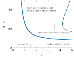
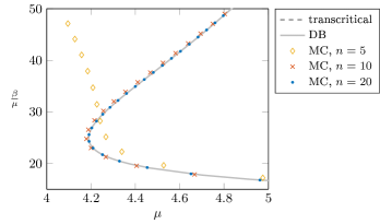
Figure 4: Stability diagram of (2.1) and its pseudospectral approximation for $\tau=1$ and $h(x)=e^{-x}$. The Hopf and period doubling bifurcation curves are approximated numerically with DDE-BIFTOOL (gray solid, DB), and MatCont (colors, MC). The right panel focusses on the approximation of the period doubling curve for different dimensions of the ODE system. We can observe the convergence of the approximated curve to that obtained with DDE-BIFTOOL when increasing the dimension $n$ (although larger dimension is required compared to the approximation of the Hopf bifurcation).

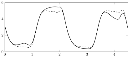
Figure 5: Periodic solutions of (2.1), approximated with MatCont and $n=20$, for $\mu=7$ and $\beta=105$ (after the period doubling bifurcation, which is detected at $\beta\approx 98.22$). The dashed line shows the periodic solution on the unstable branch (period $T\approx 2.24$); the solid line shows the periodic solution on the stable branch emerging from the period doubling bifurcation (period $T\approx 4.47$).

In the Introduction and in Section 2 we claimed that the combination of pseudospectral discretisation and MatCont enables a reliable bifurcation analysis without requiring excessive computational efforts. Indeed, by using numerical bifurcation software one can push the analysis beyond the Hopf bifurcation and approximate the branch of periodic orbits emerging from Hopf, as well as its bifurcations. The DDE (2.1), which has only one discrete point delay, can be directly analysed also by existing and well-established numerical software for delay differential equations, like DDE-BIFTOOL. We indeed use DDE-BIFTOOL as a benchmark for validating the output of the pseudospectral discretisation. In Figure 4 we show more detailed stability regions of equation (2.1) in the plane $(\mu,\frac{\beta}{\mu})$, including not only the Hopf bifurcation curve, but also the curve of period doubling bifurcations, approximated with DDE-BIFTOOL (version 3.1) and MatCont (version 7p1), running on Matlab 2019a. At the period doubling bifurcation, the branch of periodic solutions originating from the Hopf point switches stability and becomes unstable, whereas a new stable branch of periodic solutions arises. The stability change is observed from the approximated multipliers at the periodic orbit, with one multiplier exiting the unit circle and crossing -1 as $\beta$ increases. Two examples of coexisting periodic solutions are plotted in Figure 5, taken from the unstable and stable branches.

In both the package DDE-BIFTOOL and MatCont, each periodic orbit is approximated via collocation of a boundary value problem in the period interval (see for example [16, 3]). This requires the specification of a number of discretisation intervals and the degree of the collocation polynomial in each interval (we stress however that such mesh and polynomial degree are different from and independent of the mesh points and polynomial degree used to discretise the delay interval in the pseudospectral approach). In all the computations of this section we have taken a piecewise mesh of 40 intervals in the period interval, and polynomial approximations of degree 4 in each interval. These values guarantee sufficient accuracy in the approximation of the periodic orbits, so that the dominating errors in Figure 4 are those due to the chosen polynomial degree of the pseudospectral approximation.

As a further illustration we consider the system of equations

$$w^{\prime}(t) =1-\frac{kw(t)w(t-1)}{2}q(t)$$ (8.1)

$$q^{\prime}(t) =w(t)-c,$$ (8.2)

for $k,c\in\mathbb{R}_{+}$. Equations (8.1) – (8.2) correspond to a fluid flow of information between sender and receiver; $w$ refers to the average size of the sent information packages, $q$ to the average queue length and the total roundtrip time has been normalised to $1$ [23, 28].

The stability regions in the plane $(k,c)$ are plotted in Figure 6: the lower curve represents the Hopf bifurcation, whereas the upper curve is a period doubling bifurcation. Two periodic solutions are plotted in Figure 7.

Numerical software like MatCont, among their output parameters, normally return also the value of the first Lyapunov coefficient at the Hopf bifurcation. We remark, however, that the output of MatCont applied to the pseudospectral approximation can not be directly taken as approximation of the direction coefficient of the DDE, since the scaling of the left and right eigenvectors traditionally used for ODE differs from the scaling used for DDE. For DDE, indeed, the eigenvectors are scaled by taking the first component equal to 1, whereas for ODE systems the eigenvector is normalised by requiring the 2-norm to be equal 1.

So far we did not manage to treat the non-resonance condition in a completely satisfactory manner, and we explicitly assumed condition (6.16). For retarded functional differential equations, there are no roots of the characteristic equation high up the imaginary axis. So checking the non-resonance condition is executable. One would expect that for the approximating pseudospectral ODE systems similar bounds can be found, but our initial (and somewhat half-hearted) attempt to derive them failed. When the dimension of the ODE system increases, so does the number of roots. Numerical observations (also in other contexts) suggest that these ‘additional’ roots have real parts moving towards minus infinity. In particular, they do not even come close to the imaginary axis. For the ‘trivial’ DDE $y^{\prime}(t)=0$, where the ‘spurious’ eigenvalues are simply the eigenvalues of the matrix $D$, it is indeed proved that they go to minus infinity when the dimension increases [15, 35]. For more general DDE, one could try to prove that the number of roots to the right of any vertical line in the complex plane is preserved if the dimension of the approximation is large enough (in the spirit of the preservation of the dimension of the unstable manifold treated for instance in [26]). As far as we know, there are as yet no theoretical results for the pseudospectral approximation considered here.

The (numerical) bifurcation theory of delay equations is well developed, see for instance [5] and the references given there. Our analysis of the Hopf bifurcation can be seen as a proof of principle that pseudospectral approximation yields a reliable bifurcation diagram, a reliable ‘picture’. But checking the details case by case for the entire catalogue of bifurcations would, we think, provide only negligible additional insight. An attractive alternative might be to try to show, as a next step, that the centre manifold of a delay equation is (in a sense to be specified) approximated by the centre manifold of the pseudospectral ODE system.

The technical difficulties of state-dependent delay equations disappear in the pseudospectral approximation, for the very simple reason that polynomials are infinitely many times differentiable. So while here we focused on showing that known results for delay equations are well approximated by corresponding results for pseudospectral ODE, we might try to prove results for state-dependent delay equations by showing that the limit of results for pseudospectral ODE systems exists and provides information about (behaviour of) solutions of the delay equation. A concrete challenge would be to provide a rigorous underpinning for the results derived in [33].

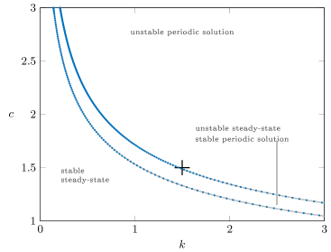
Figure 6: Stability regions of system (8.1)–(8.2) and its pseudospectral approximation, approximated with DDE-BIFTOOL (gray curve) and MatCont with $n=20$ (blue dots). The lower curve corresponds to the Hopf bifurcation, the upper curve to the period doubling bifurcation.

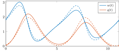
Figure 7: Periodic solutions of system (8.1)–(8.2), approximated with MatCont and $n=20$, for $c=k=1.5$ (beyond the period doubling bifurcation). The dashed line shows the periodic solution on the unstable branch (period $T\approx 5.57$); the solid line shows the periodic solution on the stable branch emerging from the period doubling bifurcation (period $T\approx 11.15$).

Appendix A Stability charts for the ‘Nicholson’s blowflies’ equation

We collect some results concerning the DDE

$$N^{\prime}(t)=-\mu N(t)+\beta N(t-1)h(N(t-1))$$ (A.1)

with parameters $\beta,\mu\geq 0$. We pay special attention to the case

$$h(x)=e^{-x}.$$ (A.2)

Equation (2.1) can be brought in the form (A.1) by scaling of time with a factor $\tau$. This entails the introduction of dimensionless parameters

$$\mu_{new}=\tau\mu_{old},\qquad\beta_{new}=\tau\beta_{old},$$

where “new” refers to (A.1) and “old” refers to (2.1). Note, incidentally, that $\beta_{old}$ also incorporates the survival of the juvenile period and that one can make this explicit by putting

$$\beta_{old}=\beta_{0}e^{-\tau\mu_{old}};$$

but we will not elaborate on this further. Finally, note that the case $h(x)=e^{-\sigma x}$ can be reduced to (A.2) by scaling of $N$ with a factor $\sigma$.

In [12] it is argued that using two parameters in Hopf bifurcation studies has great advantages. As (A.1) naturally has two parameters, we are in the ideal situation.

Nontrivial steady states $\overline{N}$ of (A.1) are characterised by the equation

$$h\left(\overline{N}\right)=\frac{\mu}{\beta}.$$ (A.3)

Under the assumptions

• $h(0)=1$;

• $h$ is monotonically decreasing;

• $\lim_{x\to\infty}h(x)=0$

equation (A.3) has a unique positive solution for $\beta>\mu$. In the parameter plane the line $\beta=\mu$ corresponds to a transcritical bifurcation. For $\beta<\mu$ the population goes extinct. For $\beta$ slightly larger than $\mu$, the nontrivial steady state is asymptotically stable. Our first aim is to investigate whether or not $\overline{N}$ can lose its stability by way of a Hopf bifurcation. See also [32] for an analysis of the occurrence of a Hopf bifurcation in system (A.1) and [36] for an analysis of the direction of this bifurcation.

As a first step we put

$$N(t)=\overline{N}+x(t)$$

and rewrite (A.1) as

$$x^{\prime}(t)=b_{1}x(t)+b_{2}x(t-1)+\mathcal{G}(x(t-1),\mu,\beta)$$

where

$$b_{1}=-\mu,\qquad b_{2}=\beta(h(\overline{N})+\overline{N}h^{\prime}(\overline{N}))$$ (A.4)

and

$$\mathcal{G}(x,\mu,\beta)=\beta\overline{N}\left(h(\overline{N}+x)-h(\overline{N})-h^{\prime}(\overline{N})x\right)+\beta\left(h(\overline{N}+x)-h(\overline{N})\right)x.$$ (A.5)

So the characteristic equation corresponding to the linearised equation reads

$$\lambda-b_{1}-b_{2}e^{-\lambda}=0.$$ (A.6)

This equation is analysed in great detail in [14, Section XI.2], to which we refer for justification of some statements below.

Substituting $\lambda=i\omega$ into (A.6) and solving for $b_{1}$ and $b_{2}$ we obtain

$$b_{1}=\frac{\omega\cos\omega}{\sin\omega},\qquad b_{2}=-\frac{\omega}{\sin\omega}.$$ (A.7)

The stability region in the $(b_{1},b_{2})$-plane is bounded by the line

$$b_{1}+b_{2}=0,\qquad b_{1}\leq 1$$

(corresponding to $\lambda=0$ being a root of (A.6)) and the curve defined by (A.7) with

$$0\leq\omega<\pi.$$ (A.8)

Note that the curve and the line intersect at $(b_{1},b_{2})=(1,-1)$ corresponding to $\lambda=0$ being a double root of (A.6). The root $\lambda=i\omega$ is simple for $\omega>0$.

If one follows a one-parameter path in the $(b_{1},b_{2})$-plane that crosses the curve defined by (A.7), (A.8) transversally, the root of (A.6) crosses the imaginary axis transversally.

There are no roots on the imaginary axis if $(b_{1},b_{2})$ is not of the form (A.7). By adjusting the domain of definition of $\omega$, one obtains via (A.7) countably many curves in the $(b_{1},b_{2})$-plane such that (A.6) has a root on the imaginary axis. These curves do not intersect the curve corresponding to (A.8) nor each other. We conclude that the non-resonance condition is satisfied. We refer to [14, Figure XI.1, page 306] for a graphical summary.

The next step is to translate the results from the $(b_{1},b_{2})$-plane to the $(\mu,\beta)$-plane or, for that matter, the $(\mu,\beta/\mu)$-plane. Here it becomes useful to adopt (A.2) since in that case (A.4) amounts to

$$b_{1}=-\mu,\qquad b_{2}=\mu\left(1-\ln\left(\frac{\beta}{\mu}\right)\right)$$

with inverse

$$\mu=-b_{1},\qquad\beta=-b_{1}e^{1+\frac{b_{2}}{b_{1}}}.$$ (A.9)

By combining (A.7), (A.8) and (A.9) we obtain the curve depicted in Figure 1, albeit in the $(\mu,\beta/\mu)$-plane. Note, however, that the interpretation requires $\mu\geq 0$ and that accordingly we should restrict to $\pi/2\leq\omega\leq\pi$.

The conclusion is that if we follow a one-parameter path in the $(\mu,\beta)$- or $(\mu,\beta/\mu)$-plane that crosses the stability boundary transversally, all assumptions of Theorem 3.2 are satisfied.

We now compute the stability boundaries for the pseudospectral approximation to (A.1). The pseudospectral approximation to (A.1) reads

$$y_{0}^{\prime}(t) =-\mu y_{0}(t)+\beta y_{n}(t)h(y_{n}(t))$$ (A.10)

$$y^{\prime}(t) =Dy(t)-D\textbf{1}y_{0}(t)$$

where we have written $(y_{0},\ldots,y_{n})=(y_{0},y)\in\mathbb{R}^{n+1}$. Equilibria of (A.1) are in one-to-one correspondence with equilibria of (A.10), so (A.10) has a non-trivial equilibrium $\overline{N}\textbf{1}$ with $h(\overline{N})=\mu/\beta$ for $\beta>\mu$. We shift the non-trivial equilibrium to zero via the coordinate transform $(y_{0},y)=\overline{N}\textbf{1}+(x_{0},x)$; then (A.10) becomes

$$x_{0}^{\prime}(t) =b_{1}x_{0}(t)+b_{2}x_{n}(t)+\mathcal{G}(x_{n}(t),\mu,\beta)$$ (A.11)

$$x^{\prime}(t) =Dx(t)-D\textbf{1}x_{0}(t)$$

with $b_{1},b_{2}$ and $\mathcal{G}$ defined in (A.4)–(A.5). The characteristic equation corresponding to the linearisation of (A.11) becomes (cf (4.20))

$$\lambda-b_{1}-b_{2}\left[(D-\lambda I)^{-1}D\textbf{1}\right]_{n}=0.$$ (A.12)

We compute the stability boundary by setting $\lambda=i\omega$ and solving for $b_{1},b_{2}$:

$$b_{1}=-\frac{\omega\mbox{Re}\,\left[(D-i\omega I)^{-1}D\textbf{1}\right]_{n}}{\mbox{Im}\,\left[(D-i\omega I)^{-1}D\textbf{1}\right]_{n}},\qquad b_{2}=\frac{\omega}{\mbox{Im}\,\left[(D-i\omega I)^{-1}D\textbf{1}\right]_{n}}.$$ (A.13)

Note that the expressions for $b_{1},b_{2}$ have singularities but at different values than the expressions for $b_{1},b_{2}$ in (A.7). By defining $h_{0}(x)=-\sin(x)$ and $h_{n}(x)=\mbox{Im}\,\left[(D-ix)^{-1}D\textbf{1}\right]_{n}$ and applying Lemma 6.1, we see that the singularities of $b_{1},b_{2}$ defined in (A.13) approximate the singularities of $b_{1},b_{2}$ defined in (A.7). Moreover, the expressions (A.13) converge to the expressions (A.7) for $n\to\infty$ and for $\omega$ in compact intervals; see Figure 10.

We now want to determine whether the root $i\omega$ crosses the imaginary axis transversely if we cross the curves (A.13) transversely. For ease of computation we restrict to varying $b_{2}$. If $i\omega$ is a simple root of (A.12), then it lies on a branch of roots $\lambda(b_{2})$ and the derivative along this branch is given by

$${\color[rgb]{0,0,0}\lambda^{\prime}(b_{2})=\frac{\left[(D-i\omega I)^{-1}D\textbf{1}\right]_{n}}{1-b_{2}\left[(D-i\omega I)^{-2}D\textbf{1}\right]_{n}}.}$$ (A.14)

with $b_{2}$ defined in (A.13). So if the real part of the right hand side of (A.14) is non-zero, the root on the imaginary axis crosses transversely if we vary $b_{2}$.

Note that by Lemma 5.1 and Corollary 5.4, $i\omega$ is a simple zero of (A.12) for $n$ large enough; moreover, the expression in (A.14) is non-zero for $n$ large enough. However, for fixed values of $n$ one has to check these conditions explicitly. We now do this for the case $n=2$.

For $n=2$, the matrices $D$ and $A_{2}$ are given by

$$D=\begin{pmatrix}0&-1\\ 4&-3\end{pmatrix},\qquad A_{2}=\begin{pmatrix}b_{1}&0&b_{2}\\ 1&0&-1\\ -1&4&-3\end{pmatrix}.$$ (A.15)

We first compute the characteristic equation for the eigenvalues of $A_{2}$. With $D$ as in (A.15), (A.12) becomes

$$\lambda-b_{1}-b_{2}\frac{4-\lambda}{\lambda^{2}+3\lambda+4}=0.$$ (A.16)

As a sanity check, we compute the eigenvalues of $A_{2}$ as roots of $\det(\lambda I-A_{2})=0$. We find that the eigenvalues are roots of the equation

$$(\lambda-b_{1})\left(\lambda^{2}+3\lambda+4\right)-b_{2}(4-\lambda)=0.$$ (A.17)

and indeed we see that the roots of (A.16) are exactly the roots of (A.17).

We now compute the stability boundary. Equation (A.17) has a root $\lambda=0$ if

$$b_{1}=-b_{2}$$ (A.18)

(the fact that steady states of DDE and the approximating ODE are in one-to-one correspondence guarantees that steady state bifurcation conditions are too). Substituting $\lambda=i\omega$ in (A.16) and solving for $b_{1},b_{2}$ (or, equivalently, computing (A.13) for $D$ as in (A.15)) gives

$$b_{1}(\omega)=\frac{7\omega^{2}-16}{\omega^{2}-16},\qquad b_{2}(\omega)=\omega^{2}-4+3\cdot\frac{7\omega^{2}-16}{\omega^{2}-16}.$$ (A.19)

Note that the expressions for $b_{1},b_{2}$ have singularities at $\omega=\pm 4$; the stability region in the $(b_{1},b_{2})$-plane is bounded by the line (A.18) and the curve define by (A.19) with

$$-4\leq\omega\leq 4;$$ (A.20)

see Figure 8.

If we cross the curve (A.19), (A.20) by varying $b_{2}$, we find that the derivative of the eigenvalue along the branch is given by

$$\lambda^{\prime}(\omega) =\frac{i\omega-4}{-3\omega^{2}+6i\omega+4-2i\omega b_{1}(\omega)-3b_{1}(\omega)+b_{2}(\omega)}$$ (A.21)

$$=\frac{i\omega-4}{\omega\left(-2\omega+6i-2b_{1}(\omega)i\right)}$$

The real part of the denominator of (A.21) is non-zero for $\omega\neq 0$; hence the denominator of (A.21) is non-zero for $\omega\neq 0$, which means that $\omega\neq 0$ is a simple zero of (A.17) for $b_{1},b_{2}$ defined in (A.19). The real part of (A.21) becomes

$$\mbox{Re}\,\lambda^{\prime}(\omega)=\frac{14-2b_{1}(\omega)}{4\omega^{2}+(6-2b_{1}(\omega))^{2}}.$$

On the interval $(-4,4)$ the expression for $b_{1}$ in (A.19) attains its maximum $b_{1}=1$ for $\omega=0$. Therefore $\mbox{Re}\,\lambda^{\prime}(\omega)\neq 0$ along the curve (A.19)–(A.20). Moreover, since $A_{2}$ has exactly three eigenvalues (counting multiplicity), the non-resonance condition is in this case easy to check. A resonance between eigenvalues $i\omega$ and $ki\omega$, $k>0$, would require 4 eigenvalues and can therefore not happen. A resonance between $i\omega$, $\omega>0$ and 0 can also not happen because the curve defined by (A.19) with $\omega\neq 0$ does not intersect the curve $b_{1}=-b_{2}$. So the conclusion is that if we cross the stability boundary (A.19) transversally, a Hopf bifurcation of system (A.10) with $n=2$ occurs.

For higher values of $n$, we can also explicitly compute the stability boundary $(b_{1},b_{2})$ as defined in (A.13). For $n=3$, the characteristic equation becomes

$$\lambda-b_{1}-b_{2}\frac{3\lambda^{2}-32\lambda+96}{3\lambda^{3}+19\lambda^{2}+64\lambda+96}=0$$

and the stability boundary as defined in (A.13) becomes

$$b_{1}(\omega)=17+\frac{2048\bigl{(}7\omega^{2}-72\bigr{)}}{9\omega^{4}-1088\omega^{2}+9216},\qquad b_{2}(\omega)=-\frac{9\omega^{6}-23\omega^{4}+448\omega^{2}+9216}{9\omega^{4}-1088\omega^{2}+9216}.$$ (A.22)

For $n\geq 4$, the formula’s can still be computed explicitly in terms of the mesh points $\theta_{j}$ but become rather long. Furthermore, for $n\geq 4$, we need numerical approximations for $\theta_{j}$ to plot the parametric curves.

We have plotted the stability boundary (A.22) together with (A.18) in Figure 9. Note that the curves defined by (A.22) and (A.18) do not self intersect and do not intersect each other; so there is never a resonance between two roots on the imaginary axis. Moreover, we see that Figure 9 has an extra curve compared to Figure 8. So it seems that the infinite number of curves defined by (A.7) get approximated one by one as we increase the discretisation index $n$.

In Figure 10 we have plotted the graphs of the functions defined by (A.13) for $n=3,4,5$. We see that for $n=3,4$, there are two curves within the depicted window. We see that as $n$ increases, the curves within the depicted window lie closer together. For $n=5$ a third curve appears in the window.

For the case where $h$ is given as in (A.2), we analyse the Lyapunov coefficient along the stability boundary for the DDE (A.1). For $\pi/2<\omega<\pi$, define the functions

$$B_{10}(\omega)=\frac{e^{-i\omega}}{1+b_{2}(\omega)e^{-i\omega}},\qquad B_{20}(\omega)=\frac{e^{-2i\omega}}{2i\omega-b_{1}(\omega)-b_{2}(\omega)e^{-2i\omega}}B_{10}(\omega)$$

with $b_{1}(\omega),b_{2}(\omega)$ as defined in (A.7). Then $c_{0}$ as defined in (3.6) becomes

$$c_{0}=\frac{1}{2}D_{1}^{3}\mathcal{G}(0,\mu,\beta)B_{10}(\omega)-\frac{(D_{1}^{2}\mathcal{G}(0,\mu,\beta))^{2}}{b_{1}+b_{2}}B_{10}(\omega)+\frac{1}{2}(D_{1}^{2}\mathcal{G}(0,\mu,\beta))^{2}B_{20}(\omega)$$ (A.23)

with

$$D_{1}^{2}\mathcal{G}(0,\mu,\beta)=\mu\ln\left(\frac{\beta}{\mu}\right)-2\mu,\qquad D_{1}^{3}\mathcal{G}(0,\mu,\beta)=-\mu\ln\left(\frac{\beta}{\mu}\right)+3\mu.$$ (A.24)

For $\pi/2<\omega<\pi$, $\mbox{Re}\,c_{0}$ is plotted in Figure 11. Note in particular that $\mbox{Re}\,c_{0}$ is always negative along the stability boundary (A.7)–(A.8).

To compute the Lyapunov coefficient of the system (A.11) when $h$ is given by (A.2), define the functions

$$B_{1n}(\omega)=\frac{\left(((D-i\omega I)^{-1}D\textbf{1})_{n}\right)^{2}\left((D+i\omega I)^{-1}D\textbf{1}\right)_{n}}{1-b_{2}(\omega)\left((D-i\omega I)^{-2}D\textbf{1}\right)_{n}},\quad B_{2n}(\omega)=\frac{\left((D-2i\omega I)^{-1}D\textbf{1}\right)_{n}}{2i\omega-b_{1}-b_{2}\left((D-i\omega I)^{-1}D\textbf{1}\right)_{n}}B_{1n}(\omega)$$

with $b_{1}(\omega),b_{2}(\omega)$ defined in (A.13). Then $c_{n}$ defined in (4.27) becomes

$$c_{n}=\frac{1}{2}D_{1}^{3}\mathcal{G}(0,\mu,\beta)B_{1n}(\omega)-\frac{(D_{1}^{2}\mathcal{G}(0,\mu,\beta))^{2}}{b_{1}+b_{2}}B_{1n}(\omega)+\frac{1}{2}(D_{1}^{2}\mathcal{G}(0,\mu,\beta))^{2}B_{2n}(\omega)$$ (A.25)

with $D_{1}^{2}\mathcal{G}(0,\mu,\beta),\ D_{1}^{3}\mathcal{G}(0,\mu,\beta)$ defined in (A.24). For $n=1,2$, we have plotted $\mbox{Re}\,c_{n}$ in Figure 11. We note that both for $n=2$ and $n=3$ the Lyapunov coefficient is negative. This reinforces our earlier conclusions that already for low values of $n$, we find good qualitative agreement between the behaviour of the DDE and the pseudospectral ODE.

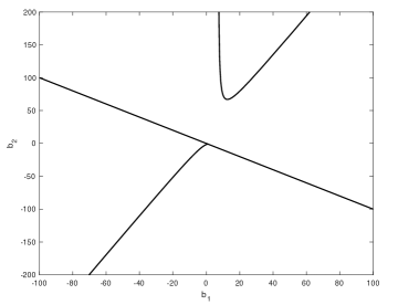
Figure 8: The curves defined by (A.18), (A.19).

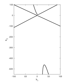
Figure 9: The curves defined by (A.18), (A.22).

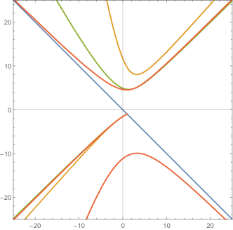
Figure 10: Parametric plot of the graphs of the functions defined by (A.13) for different values of $n$ in the $(b_{1},b_{2})$-plane: $n=3$ (brown, light, see expression (A.22)), $n=4$ (green) and $n=5$ (brown, dark). The blue line corresponds to the line defined by (A.18).

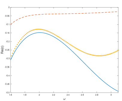
Figure 11: The Lyapunov coefficient (A.23) (blue line), and the Lyapunov coefficient (A.25) for $n=2$ (orange dashed line) and $n=3$ (yellow crosses).

References

[1]
Auto.
[2]
Knut.
[3]
A. Andò and D. Breda.
Convergence analysis of collocation methods for computing periodic
solutions of retarded functional differential equations.
SIAM J. Numer. Anal., to appear, 2020.
[4]
J-P. Berrut and L. Trefethen.
Barycentric lagrange interpolation.
SIAM Review, 46:501–517, 2004.
[5]
M.M. Bosschaert, S.G. Janssens, and Yu.A. Kuznetsov.
Switching to nonhyperbolic cycles from codimension two bifurcations
of equilibria of delay differential equations.
SIAM J. Appl. Dyn. Syst., 19:252–303, 2020.
[6]
D. Breda, O. Diekmann, M. Gyllenberg, F. Scarabel, and R. Vermiglio.
Pseudospectral discretization of nonlinear delay equations: New
prospects for numerical bifurcation analysis.
SIAM Journal on Applied Dynamical Systems, 15:1–23, 2016.
[7]
D. Breda, O. Diekmann, D. Liessi, and F. Scarabel.