Are Type Ia Supernovae in Restframe $H$ Brighter in More Massive Galaxies?

Abstract

We analyze 143 Type Ia supernovae (SNeIa) observed in $H$ band (1.6–1.8 $\mu$m) and find SNeIa are intrinsically brighter in $H$-band with increasing host galaxy stellar mass. We find SNeIa in galaxies more massive than $10^{10.43}M_{\odot}$ are $0.13\pm 0.04$ mag brighter in $H$ than SNeIa in less massive galaxies. The same set of SNeIa observed at optical wavelengths, after width-color-luminosity corrections, exhibit a $0.10\pm 0.03$ mag offset in the Hubble residuals. We observe an outlier population ($|\Delta H_{\rm max}|>0.5$ mag) in the $H$ band and show that removing the outlier population moves the mass threshold to $10^{10.65}M_{\odot}$ and reduces the step in $H$ band to $0.08\pm 0.04$ mag, but the equivalent optical mass step is increased to $0.13\pm 0.04$ mag. We conclude the outliers do not drive the brightness–host-mass correlation. Less massive galaxies preferentially host more higher-stretch SNeIa, which are intrinsically brighter and bluer. It is only after correction for width-luminosity and color-luminosity relationships that SNeIa have brighter optical Hubble residuals in more massive galaxies. Thus finding SNeIa are intrinsically brighter in $H$ in more massive galaxies is an opposite correlation to the intrinsic (pre-width-luminosity correction) optical brightness. If dust and the treatment of intrinsic color variation were the main driver of the host galaxy mass correlation, we would not expect a correlation of brighter $H$-band SNeIa in more massive galaxies.

1 Introduction

Since the late 1990s, Type Ia supernovae (SNeIa) have been used as standard candles to measure the accelerating expansion of the Universe (Riess et al., 1998; Perlmutter et al., 1999). Much work has gone into further standardizing inferred optical brightness of SNeIa by including corrections based on the stretch (Phillips, 1993) and color (Riess et al., 1996; Tripp, 1998) of the lightcurve. More recent work has started including an additional correction term associated with the stellar mass of the host galaxy of the SNeIa (Betoule et al., 2014; Scolnic et al., 2018; Brout et al., 2019; Smith et al., 2020).

Lightcurves observed at near infrared (NIR) wavelengths ($1~{}\mu$ m$<\lambda<2.5~{}\mu$ m) are more standard and require no or smaller corrections to their lightcurves to yield the same precision as optical lightcurves (Kasen, 2006; Wood-Vasey et al., 2008; Folatelli et al., 2010; Kattner et al., 2012; Barone-Nugent et al., 2012; Dhawan et al., 2018; Burns et al., 2018). We here compile one of the largest publicly available NIR SN Ia data sets to further test the standard nature of SNeIa. We explore different possible correlations between global host galaxy properties and $H$-band luminosity.

The past decade has seen an extensive history of looking for correlations between the standardized optical luminosity of SNeIa and the properties of their host galaxies. Many papers have studied relationships with global host galaxy properties such as stellar mass, metallicity, star formation rates, and age using galaxy photometry and stellar population synthesis codes (Sullivan et al., 2006; Gallagher et al., 2008; Kelly et al., 2010; Sullivan et al., 2010; Lampeitl et al., 2010; Gupta et al., 2011; D’Andrea et al., 2011; Hayden et al., 2013; Johansson et al., 2013; Childress et al., 2013a, b; Moreno-Raya et al., 2016; Campbell et al., 2016; Wolf et al., 2016; Roman et al., 2018; Uddin et al., 2017a; Jones et al., 2018; Rose et al., 2019). These papers have found several correlations between standardized brightness and host galaxy properties with the most significant one being host galaxy stellar mass. Some interpret this as a result of a correlation between galaxy stellar mass and things more physically related to the SN Ia explosion, such as progenitor metallicity, progenitor age, or dust (Kelly et al., 2010; Hayden et al., 2013; Childress et al., 2013b; Brout & Scolnic, 2020). These analyses show that the standardized brightness of SNeIa hosted in higher-mass galaxies is brighter by $\sim$0.08 mag (Childress et al., 2013b) than SNeIa hosted in galaxies with stellar mass less than $10^{10}M_{\odot}$. The mass “step” was also implemented in one of the recent studies to produce cosmological constraints: the Joint Lightcurve Analysis (JLA; Betoule et al., 2014), where they independently measured a correlation with host galaxy stellar mass and implemented a step function to account for it. Others have focused on local properties of host galaxies such as recent star formation rates within 1–5 kpc of the supernova position using spectroscopy or ultraviolet (UV) photometry (Rigault et al., 2013, 2015, 2018; Kelly et al., 2015; Uddin et al., 2017b). These local property studies find that the standardized brightness of SNeIa in locally passive regions is $\sim$0.094 mag (Rigault et al., 2015) brighter than those in locally star forming regions. Furthermore, Kelly et al. (2015) showed that SNeIa in locally star forming regions were more standard than those in non-star forming ones.

However, not every analysis suggests that there is a correlation with host galaxy properties. Kim et al. (2014) used an updated lightcurve analysis that is more flexible to intrinsic variations in SNeIa (introduced in Kim et al., 2013) and found any potential correlations with host galaxy stellar mass, specific star formation rates, and metallicity to be consistent with zero. Jones et al. (2015) found no evidence of a correlation between host galaxy local star formation rates derived from UV photometry by using a larger sample size than previous studies and using different selection criteria. Scolnic et al. (2014) described the systematics utilized in the Pan-STARRS SN Ia cosmology analysis (Rest et al., 2014) and found a correlation with host galaxy stellar mass with a step size of $0.037\pm 0.032$ mag, which is consistent with 0 and is 2-$\sigma$ inconsistent with the previously reported sizes in the literature of $\sim 0.1$ mag. With twice as many SNeIa, the subsequent Pan-STARRS analysis (Scolnic et al., 2018) recovered a very similar small step size of $0.039\pm 0.016$ mag, but now with a clear deviation from 0. Scolnic et al. (2018) noted that if they did not apply the BEAMS with Bias Correction (BBC; Kessler & Scolnic, 2017) method in their analysis they would have found a mass step of $0.064\pm 0.018$ mag. The Dark Energy Survey (DES; Dark Energy Survey Collaboration et al., 2016; Abbott et al., 2019; Brout et al., 2019) originally found no evidence of a host galaxy stellar mass step for 329 SNeIa with 207 observed in the first three years of DES and the rest from low-redshift samples. However, Smith et al. (2020) showed that the DES data do exhibit a mass step if a JLA-like analysis is run, which strongly suggests that such a mass step was being corrected for by the BBC method used in the DES SN cosmology papers to date.

We see much evidence to warrant continued exploration of this parameter space to understand whether we are searching for a real correlation or if we need to improve the analysis of SNeIa lightcurves.

The majority of the previous analyses of host galaxy properties versus SN Ia corrected brightness have examined correlations using only optical lightcurves. Doing a similar analysis using NIR lightcurves will help shed light on physical mechanisms and color-dependent intrinsic dispersions. For example, the NIR is less sensitive to dust such that if there is no correlation found in the NIR, but a correlation found at optical wavelengths, it would provide evidence that the host mass correlation is actually an unaccounted for dust correlation.

In the restframe NIR there have been far fewer studies of host galaxy correlations. Dhawan et al. (2018) looked at the $J$-band and, with a small sample of 30 SNeIa, found low dispersion ($\sim 0.10$ mag) and no obvious trend with host galaxy morphology. A more in-depth study was done using the Carnegie Supernova Project (CSP) sample by Burns et al. (2018), which compared $H$-band brightnesses to host galaxy stellar mass estimates from $K$-band photometry following the mass-to-light ratio method of McGaugh & Schombert (2014). Uddin et al. (2020) expanded this analysis to examine correlations from optical to NIR lightcurves with new observations of each host galaxy. Uddin et al. (2020) found a small $\sim 1\sigma$ linear correlation and $\sim 2\sigma$ step function ($0.093\pm 0.043$ mag) between the restframe $H$-band and host galaxy stellar mass for their sample of $113$ SNeIa. We here analyze a data set with significantly more SN Ia in low-mass host galaxies, $M<10^{10}M_{\sun}$, the canonical break point for the mass step.

SNeIa in the $H$-band have been shown to be standard to $0.15$–$0.2$ mag without lightcurve corrections (Wood-Vasey et al., 2008; Folatelli et al., 2010; Barone-Nugent et al., 2012; Kattner et al., 2012; Weyant et al., 2014; Stanishev et al., 2018; Avelino et al., 2019) whereas optical lightcurves before brightness standardization have significantly larger scatter of $\sim 0.8$ mag (Hamuy et al., 1995). However, there are only $\sim$220 NIR lightcurves publicly available compared to the over $>1,000$ available for optically observed SNeIa.

We use SNooPy (Burns et al., 2011, 2014) for lightcurve fits as it is has the most developed treatment of NIR templates. We combine optical and NIR lightcurves to improve fits with the $s_{BV}$ parameter from Burns et al. (2014). Most previous analyses have explored host galaxy correlations with standardized brightnesses calculated from SALT2 (Guy et al., 2007) and/or MLCS2k2 (Jha et al., 2007) fitters (e.g., Kelly et al., 2010).

This paper is organized as follows: Section 2 explains the supernova sample we use and how we collected optical, UV, and NIR photometry of the host galaxies. Section 3 details how we fit lightcurves and created the restframe $H$-band and optical Hubble diagrams. Section 4 examines the host galaxy stellar mass correlation and shows that the $H$-band Hubble residuals and the optical width-luminosity corrected Hubble residuals are both more negative in higher-mass galaxies. Section 5 explores the statistical significance of these correlations. We present our conclusions and recommendations for future work in Section 6.

2 SN Ia and Host Galaxy Sample

The improved ability to determine standard distances, together with the reduced sensitivity to dust extinction, have motivated several recent projects to pursue larger samples of SNeIa observed in the restframe NIR: CSP-I, II (Contreras et al., 2010; Stritzinger et al., 2011; Kattner et al., 2012; Krisciunas et al., 2017; Phillips et al., 2019); CfA (Wood-Vasey et al., 2008; Friedman et al., 2015); RAISINS (Kirshner, 2012); SweetSpot (Weyant et al., 2014, 2018); and SIRAH (Jha et al., 2019). Section 2.1 overviews the NIR sample currently available and used in this analysis.

To gather host galaxy properties, we used publicly available galaxy catalogs from Sloan Digital Sky Survey (SDSS), Panoramic Survey Telescope and Rapid Response System (Pan-STARRS), DECam Legacy Survey (DECaLS), Galaxy Evolution Explorer (GALEX), and Two Micron All-Sky Survey (2MASS). We used kcorrect (Blanton & Roweis, 2007) to estimate estimate galaxy properties including the stellar mass of the host galaxies. We detail this process in Section 2.2.

2.1 SNeIa

We start with the compilation of literature SNeIa gathered in Weyant et al. (2014). We assigned each SN Ia to “belong” to a given survey to be able to examine properties as a function of survey. If a SN Ia was found in multiple surveys, we labeled that object with the survey name containing the most lightcurve points in $H$; however, lightcurve points from all surveys were included when running the lightcurve fits. We used the following survey codes: K+, CSP, BN12, F15, W18.

• K+ is the miscellaneous early sample (Jha et al., 1999; Hernandez et al., 2000; Krisciunas et al., 2000, 2003, 2004a, 2004b, 2007; Valentini et al., 2003; Phillips et al., 2006; Pastorello et al., 2007a, b; Stanishev et al., 2007; Pignata et al., 2008) and named for extensive early work by Kevin Krisciunas and originally defined in Weyant et al. (2014).

• CSP refers to the lightcurves released from Contreras et al. (2010, C10) and Stritzinger et al. (2011, S11). There were NIR observations of 71 SNeIa in the C10+S11 samples. One of these, SN 2004eo, is placed in the K+ sample and 11 are placed in the CfA sample.

• BN12 covers the SNeIa from Barone-Nugent et al. (2012).

• We renamed the CfA sample from WV08 (Wood-Vasey et al., 2008) to F15 due to the 74 additional SNeIa from the final data release (Friedman et al., 2015). We do not use any of the peculiar Iax supernovae (Foley et al., 2013) from Friedman et al. (2015). 5 of the F15 SNeIa overlap with and are placed in the CSP sample and 1 F15 SN Ia is placed in the BN12 sample.

• The SweetSpot W14 sample is replaced by W18 due to the addition of 34 SNeIa from SweetSpot’s first data release (Weyant et al., 2018).

All of the SNeIa from BN12 were discovered in the non-targeted PTF survey. The other samples here have SNeIa mostly discovered in surveys targeted on known galaxies.

Our full sample of SNeIa $H$-band lightcurves consists of 220 SNeIa. Table 1 gives the breakdown per survey. We used the Open Supernova Catalog (OSC; Guillochon et al., 2017) to retrieve all lightcurve data. We inspected the filter choices and definitions listed in the OSC compilation and spot-checked data against the published tables in the original papers.

We removed the 10 91bg-like SNeIa, two 02cx-like SNeIa, and two more generically peculiar SNeIa as reported in their classification spectra. We removed SN 2011aa because its lightcurve in F15 seems to be in error as its almost flat over 40 days in $J$, $H$, and $K$. We then fit these SNeIa with SNooPy (see Section 3). In order to be included on the Hubble diagram, a supernova was required to have at least 3 observations with a signal-to-noise greater than 3.5 and have a fit with a chi-square per degree of freedom less than 3. These cuts removed 41 SNeIa nominally successful SNooPy fits. Table 1 shows how many SNeIa have lightcurve fits that pass the quality cuts (“Pass LC Fit Cuts”). The left side of Figure 1 shows the redshift distribution of the full sample compared to the distribution of the Hubble diagram sample used for the analysis below. The full sample has a median redshift of 0.026 while the Hubble diagram sample has a slightly lower median redshift of 0.022.

We were not able to obtain reliable host galaxy photometry for SN 2004S. Thus out of the 144 SNeIa, 143 have sufficient host galaxy photometry to derive stellar masses (see Section 2.2).

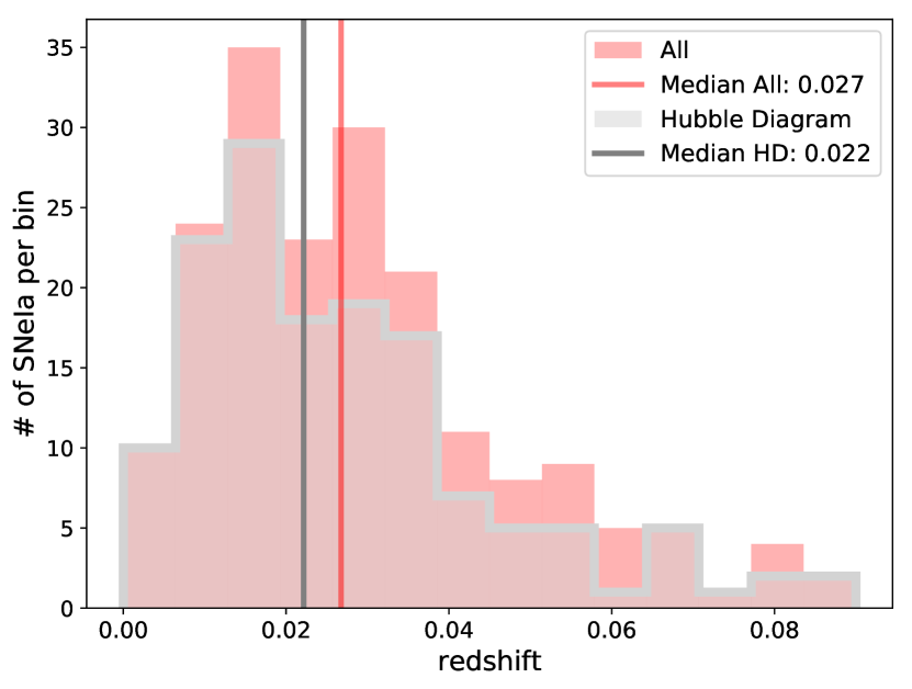
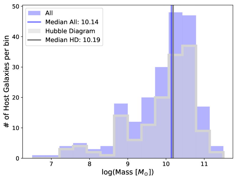
Figure 1: Left: Redshift distribution of the publicly available NIR sample of 220 SNeIa and the Hubble Diagram sample of 144 SNeIa. Right: Mass distribution of the host galaxies in log space of the publicly available NIR sample and the Hubble Diagram sample.

The right side of Figure 1 compares the mass distribution of the full sample versus those SNe Ia that are in the Hubble diagram sample. The medians for both distributions are comparable and the distribution shapes are consistent. Table 1 details how many SNeIa each sample have a successful SNooPy lightcurve fit, pass the quality cuts, and have sufficient information to calculate a host stellar mass (“Pass LC + Host Mass”).

For all 220 SNeIa with $H$-band lightcurves, we used the OSC to download any available corresponding optical lightcurves. Some surveys such as CSP and F15 obtained complementary optical lightcurves as a part of their survey; however, other surveys such as BN12 and W18 did not. All optical lightcurves go through the same quality cuts as the the NIR sample. 103 SNeIa observed in optical wavelengths passed the LC fit cuts and had usable host galaxy masses. The optical sample contains 99 SNeIa that are also in the NIR sample.

Table 1: Number of SNeIa from NIR Surveys

SN Survey	Total	Pass LC Fit Cuts	Pass LC+Host Mass
K+	23	11	10
CSP	59	47	47
BN12	12	12	12
F15	92	56	56
W18	34	18	18
Total	220	144	143

2.2 Host Galaxies

The host galaxy for all 220 SNeIa was identified from the IAU list of supernovae and the NASA Extragalactic Database (NED). The procedure to confirm a host galaxy started with either the suggested host from the transient announcement or a distance search in NED. We confirmed each host redshift matched the supernova redshift and visually examined other potential hosts in the vicinity. We used NED to collect the host galaxy name, coordinates, and the heliocentric redshift for each galaxy. If NED did not have a spectroscopic redshift, we recorded the redshift of the hosted supernova from the classification spectrum.

We obtained optical photometry from the SDSS Data Release 13 (SDSS Collaboration et al., 2016), the DECam Legacy Survey (DECaLS; Dey et al., 2019), and the Pan-STARRS1 Data Release 2 (PS1; Chambers et al., 2016; Flewelling et al., 2016; Magnier et al., 2016). The SDSS and PS1 photometry were downloaded using their respective CasJobs websites. For SDSS photometry, we used the $ugriz$ “modelMag” magnitudes, which are based on the best fit de Vaucouleurs or Exponential profile in the $r$-band. Though “cmodelMag” magnitudes give a more accurate description of the total flux in each filter, “modelMag” magnitudes are better for color studies because the flux is measured consistently across all filters (Stoughton et al., 2002).

We also obtained the PS1 stacked Kron (Kron, 1980) magnitudes, which uses the first moment of an image to determine the radius out to which flux should be integrated. This photometry and the masses derived using them are referred to as “PS1”. PS1 does not always have all five $grizy$ magnitudes for all of our objects. If $gi$ magnitudes were not available in PS1, we did not use that host galaxy photometry as we could not calculate extinction coefficients (Tonry et al., 2012).

We used the Astro Data Lab at NSF’s National Optical-Infrared Astronomy Research Laboratory cross-match service to query the DECaLS catalog. DECaLS uses Tractor (Lang et al., 2016) to fit a morphological type to each source and then extracts the photometry measured in AB magnitudes This method is conceptually similar to what is done in SDSS. We only use the optical filters available ($grz$) from DECaLS.

We obtained GALEX GR6/GR7 (Bianchi et al., 2014) far ultraviolet (FUV/$F$) and near ultraviolet (NUV/$N$) information where available from the MAST data archive. We used the photometry that is the result of the elliptical aperture method “MAG$\_$AUTO”, which is similar to the Kron radius calculation, in Source Extractor (Bertin & Arnouts, 1996). GALEX often reported detections in only one of FUV or NUV magnitudes, but we only required one of these to mark an object as having UV data.

We also gathered $JHK_{s}$ magnitudes from the 2MASS All-Sky Extended Source Catalog (XSC; Skrutskie et al., 2006) using the NASA/IPAC Infrared Science Archive (IRSA). We used the total magnitude calculated from the extrapolated radial surface brightness profile. One object (PGC 1361264, host of SN 2010ho) had an $H$-band uncertainty of zero and a magnitude significantly inconsistent with its $JK_{s}$ magnitudes, so that $H$-band photometric point was not used to determine the mass of PGC 1361264.

There were 5 galaxies that did not have optical photometry in any of these three surveys or GALEX UV photometry and measurements only from 2MASS were not sufficient to get a reliable host galaxy mass. We supplemented those 5 galaxies with optical photometry from Uddin et al. (2020, U20 hereafter). U20 compared their galaxy photometry with SDSS and derived the best fit linear offsets (U20 Table 1). We applied these offsets to their photometry and treated them as SDSS measurements to determine host galaxy mass. This set of host galaxies is labeled as “CSP Host Phot” to distinguish it from the CSP subsample of SNeIa.

We use kcorrect (Blanton et al., 2003; Blanton & Roweis, 2007) to transform the photometry to the restframe and infer physical parameters such as stellar mass. kcorrect fits galaxy spectral energy distributions from the UV to NIR and relies on Bruzual & Charlot (2003) stellar evolution synthesis models using the Chabrier (2003) stellar initial mass function (IMF). The physical parameters that kcorrect reports are based on those of the galaxy templates from these models. Adding the UV and NIR photometry to the optical photometry gives sharper constraints on dust absorption and thus help distinguish the different galaxy models that overlap at optical wavelengths. Figure 2 shows an example where a spiral and elliptical galaxy largely agree in optical wavelengths, but are clearly distinguished with the addition of UV and NIR measurements. All magnitudes are converted to the AB magnitude system and are extinction corrected for Milky Way dust before being input into kcorrect. We derive $K$-corrections and host galaxy stellar mass by combining optical photometry plus GALEX and 2MASS for each host galaxy. If there was no optical photometry, we required the galaxy to have four observations between GALEX and 2MASS to ensure at least one point in the UV and in the NIR. Table 2 lists how many SN Ia host galaxies have photometry for each of the surveys that are in our analysis.

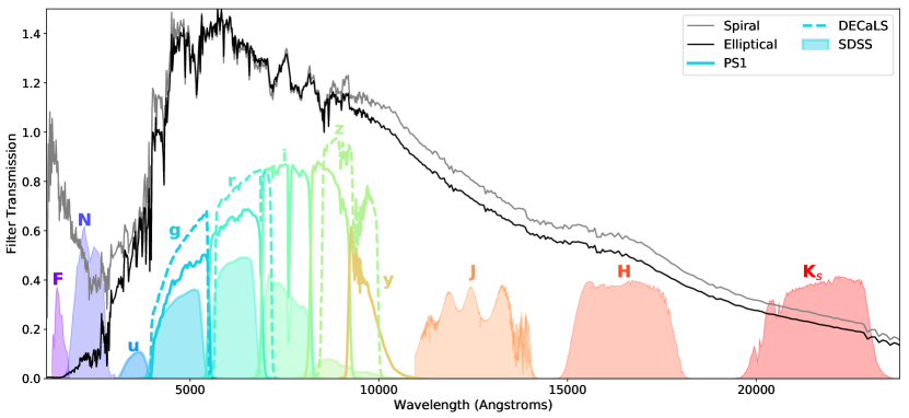
Figure 2: System transmission functions for GALEX ($F$, $N$), SDSS ($ugriz$), DECaLS ($grz$), PS1 ($grizy$), and 2MASS ($JHK_{s}$). These transmission functions accounts for the detector, optics, filter, and atmosphere. Over-plotted is the normalized spectral energy distribution (SED) for a Sc spiral galaxy in grey and an elliptical galaxy in black from the SWIRE Template Library (Polletta et al., 2007). For both spiral and elliptical galaxies, the majority of their flux is emitted at restframe optical wavelengths peaking in $gri$ bands. The Sc spiral galaxies have a small bulge and obvious spiral arms containing young stars emitting heavily in the UV. Though having optical photometry observes most of the flux, observing UV and NIR can help constrain the spectrum.

Figure 2 illustrates the wavelength coverage from these surveys. All 144 lightcurves have host galaxy photometry available in at least one of these catalogs but only 143 galaxies meet our requirement for a robust host galaxy stellar mass measurement. The redshift and host galaxy mass distributions of our final sample versus the full sample is presented in of Figure 1.

Figure 3 shows a histogram of the galaxies in the Hubble diagram sample that have photometry in each survey. There is a large overlap between the galaxies observed by SDSS, DECaLS, PS1, and CSP Host Phot. Figure 4 shows the final breakdown of photometry used in this analysis. We preferentially chose SDSS over DECaLS over PS1 (See Section 2.2.2). We summarize the photometric data in Table 14 for all 220 SNeIa.

Table 2: Number of Host Galaxies Observed in Our Sample per Galaxy Catalog.

Sample	Survey	Optical	GALEX	2MASS	GALEX+2MASS	Total
All	SDSS	14	14	14	55	97
	DECaLS	7	2	18	32	59
	PS1	3	1	16	21	41
	CSP Host Phot	0	0	5	0	5
	None	$\cdots$	$\cdots$	2	16	18
	Total	24	17	55	124	220
Hubble	SDSS	9	8	10	32	59
Diagram	DECaLS	4	2	14	19	39
	PS1	3	0	13	15	31
	CSP Host Phot	0	0	5	0	5
	None	$\cdots$	$\cdots$	1	9	10
	Total	16	10	43	75	144

Note. — The Survey column denotes in which survey the optical photometry was used. The Optical column presents how many objects had only optical data. The GALEX column are galaxies with optical and UV observations. The 2MASS column are galaxies with optical and NIR observations. The GALEX+2MASS column presents how many galaxies have observations in all three optical, UV, and NIR catalogs.

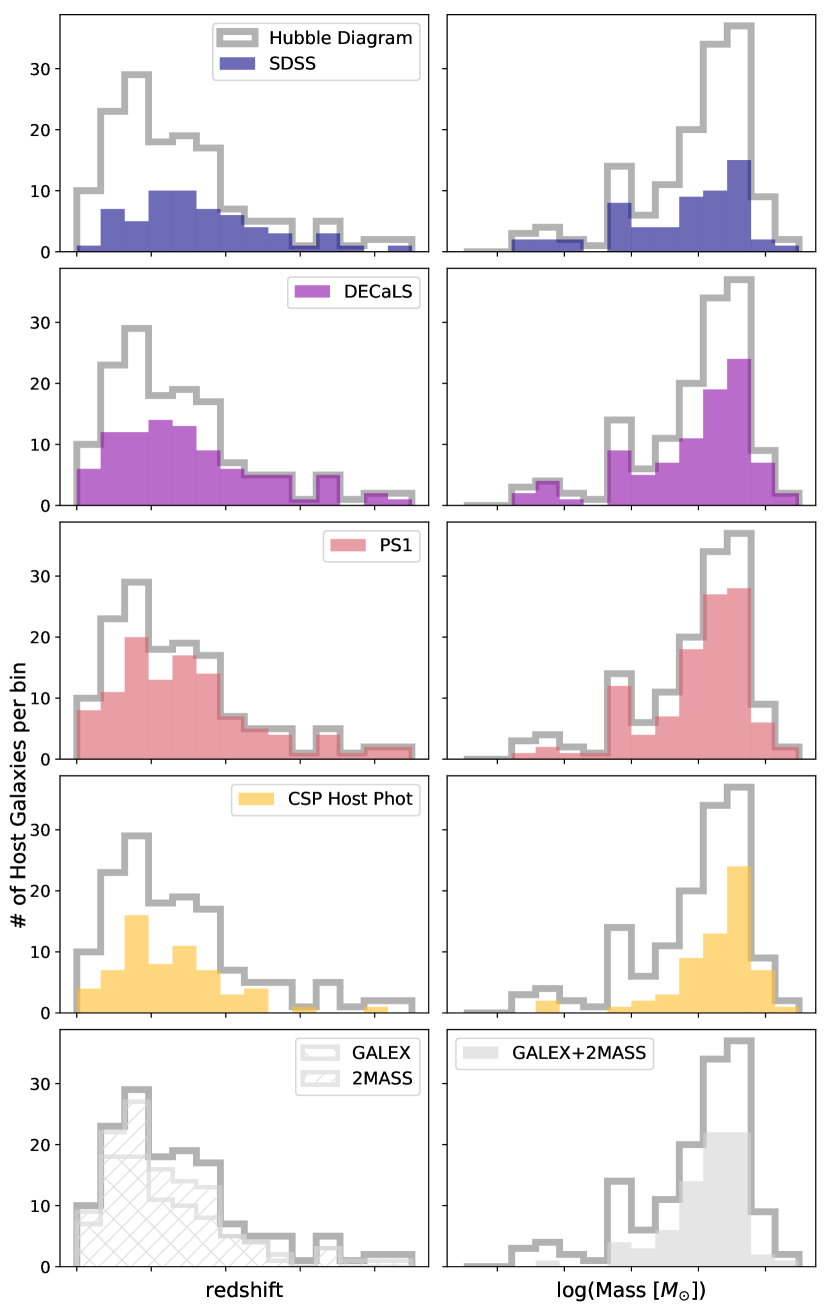
Figure 3: The redshift (left) and host galaxy mass (right) histograms of the total available host galaxy photometry in SDSS, DECaLS, PS1, and CSP Host Phot for the 144 SNeIa used in the Hubble diagram analysis, which is outlined in grey for all plots. The bottom left histogram shows the total coverage in redshift for GALEX and 2MASS separately; however, in the bottom right mass histogram we required both GALEX and 2MASS measurements to ensure more reliable mass measurements.

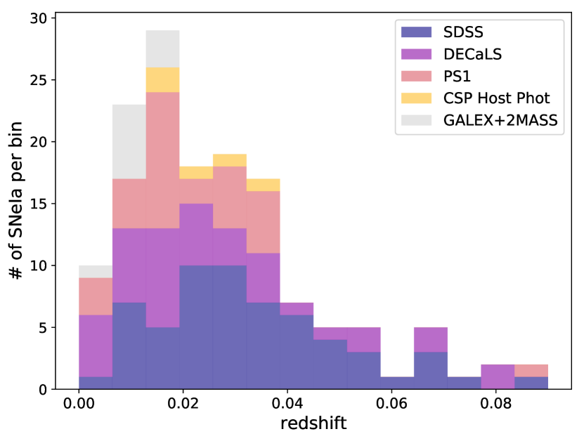
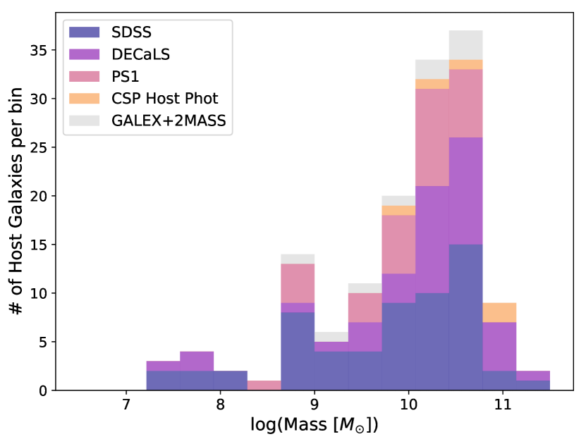
Figure 4: Left: Redshift distribution identifying which survey’s photometry was used to determine the host galaxy mass the final sample of 144 SNeIa used in the Hubble residual analysis. In addition to optical photometry, most host galaxies also have photometry in GALEX and/or 2MASS but the grey “GALEX+2MASS” indicates that no optical photometry was used to determine the mass. Right: Mass distribution of the 143 host galaxies in log space separated by which survey was used to determine the mass.

2.2.1 Special Cases for Optical Galaxy Photometry

A few galaxies observed by SDSS and PS1 could not be handled using the normal catalog searches. In SDSS, the host galaxy for SN 2011fe is M101. SN 2011fe was not used in the Hubble diagram analysis, but the mass was used in Figure 1. We had to use special large galaxy catalogs for SDSS (DR7; Adelman-McCarthy & et al., 2009), the GALEX Ultraviolet Atlas of Nearby Galaxies (Gil de Paz et al., 2007), the 2MASS Large Galaxy Atlas (Jarrett et al., 2003).

In PS1, there are two objects that are in galaxy pairs: SN 2007sr located in the Antennae Galaxies (NGC 4038/NGC 4039) and SN 2011aa located in UGC 3906. For both of these, we kept photometry for each galaxy and averaged the host galaxy mass from kcorrect. SN 2011aa is not used in the Hubble diagram analysis.

Three host galaxies had observations in PS1 but no associated catalog photometry. Here we list the galaxy, associated supernova, and probable cause for the failure of a catalog measurement:

1. UGC 3329, SN 1999ek, Two bright stars in the foreground;

2. Unnamed host of PTF13dad, Galaxy is faint;

3. Unnamed host of PS1-13dkh, There is a live SN in the images and has a bright star nearby.

After masking the bright stars and SN, we performed aperture photometry from a derived Kron radius using the calibration information provided by PS1. We counted these as PS1 magnitudes.

The host galaxy for SN 2004S (ESO 427-G6) did have some imaging from PS1, but it was at a low declination causing the survey to cut off close to the observation. No catalog information was available and we were unable to use these images with our own algorithms. ESO 427-G6 was also missing information from GALEX and 2MASS-only photometry is not sufficient to measure a mass. This is the only object missing a mass estimate in the Hubble sample. NGC 4679, the host of SN 2001cz, was not used in the Hubble diagram analysis but should have been included in Figure 1; however, it only has measurements from 2MASS and was excluded.

If any of the surveys observed a host galaxy when the respective SN Ia was active, the SN Ia could contaminate the measured flux. We cross matched the years that SDSS, PS1, DECaLS, GALEX, and 2MASS were active with the time of maximum light of our supernovae and examined the respective galaxy images if there was an overlap in time. The only contamination (PS1-13dkh in PS1) we discovered was already accounted for in this section.

2.2.2 Comparing Masses Derived using Different Surveys

We used galaxies in Stripe 82 (Abazajian et al., 2009) at redshifts between 0.001 and 0.1 to compare the masses derived with photometry from different optical surveys. We downloaded the galaxies from SDSS and then matched on their coordinates to catalogs from DECaLS, PS1, GALEX, and 2MASS. The different sets of optical photometry were used in kcorrect to derive masses, as is done for the SNeIa host galaxies. We also compared different combinations of data including only optical data, optical plus GALEX plus 2MASS, optical plus GALEX, and optical plus 2MASS.

Figure 5 shows the mass histograms for the Stripe 82 galaxies for the different combinations of multi-wavelength photometry. Each photometry combination in the different frames contains the same galaxies such that each frame is comparing the same set of objects. Table 3 shows the number of galaxies used in each frame. Overlaid on each frame is are the galaxy mass measurements for objects with no optical photometry. These mass measurements are required to have both GALEX and 2MASS information; however, this excludes many low mass objects from our comparison as they are too dim to be detected by 2MASS. For the optical photometry-only mass measurements, the low mass galaxies observed with DECaLS and PS1 follow the same distribution relative to SDSS as the higher mass galaxies.

Figure 5: Left: Masses derived for galaxies in Stripe 82. Top left is using only optical photometry. Top right uses optical photometry and GALEX and 2MASS. Bottom left uses only optical and GALEX photometry. Bottom right uses only optical and 2MASS photometry. For comparison, we have also included the histogram for the GALEX+2MASS (“GX+2M”) derived masses where no optical photometry is used. The legends contain the median mass in log solar masses. Right: The difference between the median mass derived with photometry from DECaLS, PS1, and GALEX+2MASS (no optical) compared to the median mass from SDSS. Each set of comparisons corresponds to a frame on the left side of this figure. The error bars are the 16th and 84th ($1~{}\sigma$) percentiles. The grey area corresponds to the estimated error on galaxy mass at 0.32 dex (Section 2.2.4).

The right side of Figure 5 shows the difference of each optical photometry source compared to SDSS with the estimated error on SDSS mass in grey (see Section 2.2.4). It further shows how each survey difference changes depending on which supplementary photometry is included. In all cases, DECaLS has a nearly zero median offset from SDSS indicating that it is the most similar to kcorrect masses derived with SDSS photometry. PS1 is systematically offset to lower masses.

To determine how the surveys differ in a one-to-one galaxy mass comparison, we calculated the root mean square (RMS) error while taking the measurement from SDSS to be the truth. Table 3 summarizes these results and shows that DECaLS is consistently more aligned with SDSS than PS1. Though the distribution of masses for GALEX+2MASS aligns slightly better with SDSS than PS1 (Figure 5), PS1 does better when comparing individual galaxies.

Table 3: RMS Difference in Mass Compared to SDSS for Stripe 82 Galaxies.

Photometry Combination	$\#$	PS1	DECaLS	GALEX+2MASS
Optical Only	2603	0.18	0.14	0.17
GALEX + Optical + 2MASS	1627	0.16	0.13	0.18
GALEX + Optical	1627	0.18	0.16	0.19
Optical + 2MASS	2601	0.16	0.13	0.17

Note. — RMS units in $\log_{10}(M_{\odot})$

Since kcorrect was intended to be used for SDSS photometric observations, we gave priority to SDSS photometry first. Comparing other optical photometry to SDSS, we preferentially used the DECaLS optical photometry for objects without SDSS photometry. We then used PS1 if neither SDSS nor DECaLS photometry were available. We give the lowest priority to observations without optical photometry. Table 2 gives the final number breakdown for which optical photometry was used.

Figure 6 compares kcorrect-derived properties for SDSS versus SDSS+UV, SDSS+NIR, or SDSS+UV+NIR for the 1627 Stripe 82 galaxies with optical, GALEX, and 2MASS photometry. All the optical surveys show similar correlations as SDSS does in this figure. The high-mass galaxies agree with the optical-only measurements, because they have less dust and star formation such that the mass-age degeneracy that is broken by adding UV and/or NIR information is less relevant. At masses $<10^{10}M_{\odot}$, there are differences between the SDSS-only and SDSS+ results with additional discrepancies between SDSS+UV versus SDSS+NIR in the derived mass. Adding UV and NIR wavelength coverage improves estimates of low mass galaxies as long as the templates cover the same parameter space. GALEX+2MASS is the most discrepant, but as shown in Figure 5, the overall distribution is in agreement with SDSS and the errors are within the estimated mass error.

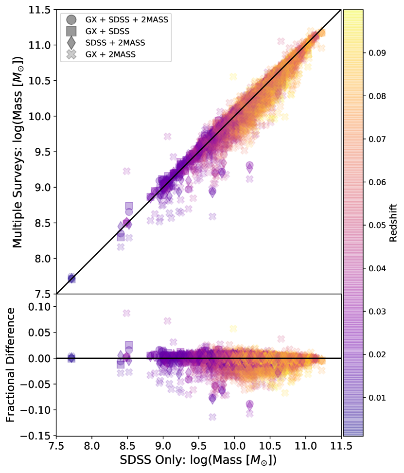
Figure 6: Comparison of the derived mass from kcorrect for Stripe 82 galaxies when only optical SDSS data is used versus GALEX+SDSS+2MASS (squares), GALEX+SDSS (circles), SDSS+2MASS (diamonds), and GALEX+2MASS (x). Top: One-to-one mass comparisons. Bottom: Fractional difference between the SDSS-only derived masses and the masses derived from other or additional sources. The color map indicates the redshift of the host galaxy. Most high mass galaxies are in agreement with the optical only measurements; however, low mass galaxies show more variation.

Though the photometry should be similar to SDSS, we compared the CSP host galaxy photometry masses derived using kcorrect to those calculated using SDSS and DECaLS photometry in Figure 7. We cannot use Stripe 82 galaxies in this comparison, so we used the 29 host galaxies that overlap between U20 and this paper’s sample. The median offset between SDSS (DECaLS) photometry-derived masses and CSP photometry-derived masses is 0.022 (0.035) dex. These offsets are well within the estimated errors that we derive for kcorrect in Section 2.2.4.

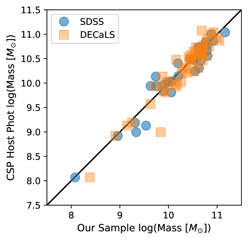
Figure 7: Comparison of masses derived from kcorrect using SDSS (circles) and DECaLS (squares) photometry versus CSP photometry. Median offset of 0.022-0.035 dex. Standard deviation of 0.18-0.34 dex. These offsets are well within the estimated errors that we derive for kcorrect in Section 2.2.4. The black line is a one-to-one comparison to guide the eye.

Of the 29 host galaxies in common with the U20 derived masses, one host mass derived using CSP photometry APMUKS(BJ) B051529.79-235009.8 for SN 2006is had a discrepancy of almost $2~{}\log(M_{\odot})$ compared to the mass determined using DECaLS. The galaxy is very faint with only $griJ$ observations from U20. No other object in the CSP sample is missing both $u$ and $H$ measurements. The DECaLS derived mass matches within the error bar of the U20 mass measurement. All 5 galaxies from U20 used in this analysis have a mass equal to or greater than $10^{10}$ and $ugriJH$ (one is missing $u$) and should be consistent with the other surveys.

2.2.3 Aperture Photometry from Different Surveys

When using photometry from the different surveys, we did not extract new photometry with equivalent effective radii to ensure that each survey was measuring the same area of flux.

SDSS and DECaLS are calculated in similar ways such that each object is fit with an exponential profile and a de Vaucouleurs profile. We downloaded all of the measured effective radii for the Stripe 82 galaxies. We then sorted the effective radii into groups based on whether they were classified as having an exponential profile or a de Vaucouleurs profile. Figure 8 shows a one-to-one comparison of effective radii for DECaLS versus SDSS effective radii. There is a tight correlation with the SDSS radius with a median difference of approximately zero, specifically $-0.02\pm 0.01^{\prime\prime}$. The outliers at low magnitudes ($\sim 22$ mag) correspond to very small and dim galaxies in SDSS that were not detected in DECaLS but did have a brighter object nearby. In some cases the dim objects are subsections of larger galaxies in SDSS that are matched the whole galaxy in DECaLS. Large ($>10$″) outliers are due to crowded fields, mix-ups in object identification, extremely faint objects, clumpy/highly structured objects, or irregular shaped galaxies that confuse the algorithms. We visually inspected images for all of the galaxies in our sample to check for possible erroneous magnitude measurements. In general, these two surveys are using similar effective radii to SDSS to do their aperture photometry.

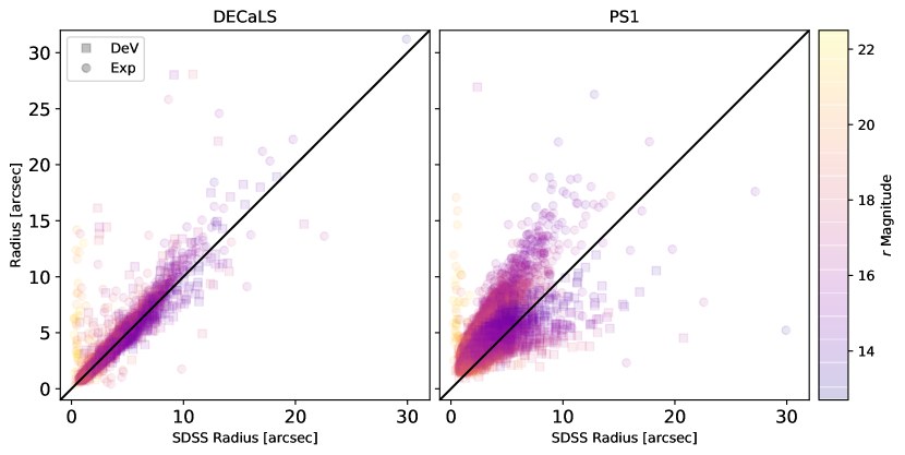
Figure 8: One-to-one comparison of the effective radii compared to SDSS for DECaLS and PS1. The squares correspond to a de Vaucouleurs (DeV) profile fit and the circules correspond to an Exponential (Exp) profile fit. The color scheme corresponds to the SDSS $r$ model magnitude. The black line is a one-to-one comparison to guide the eye. The dim objects with small radii in SDSS and large radii in the other surveys are mismatches between the surveys. The SDSS objects are typically small galaxies that are too faint for DECaLS or PS1. The PS1 Kron radii have been adjusted to account for the DeV or Exp scaling factor provided in Graham & Driver (2005).

The PS1 sample uses Kron magnitudes that are measured using a different algorithm than the other optical photometry. They are measured using the first radial moment and contains $~{}90\%$ of the total flux. We expect the total flux to be underestimated and we see from Figure 5 that the PS1 mass measurements are systematically offset by about 0.1 dex. To compare the Kron radii to the effective radii for the profile fitting from the other surveys, we use the relationships from Graham & Driver (2005) for the exponential ($r_{\rm Kron}=1.19r_{\rm effective}$) and de Vaucouleurs ($r_{\rm Kron}=2.29r_{\rm effective}$) profile. We applied these two corrections and compared the two profiles in Figure 8. There is a much larger scatter and offset compared to SDSS than with DECaLS with a median and standard deviation of $-2.32\pm 0.41^{\prime\prime}$ for the exponential profile and $-0.62\pm 0.24^{\prime\prime}$ for the de Vaucouleurs profile.

Though there are differences in the photometry from the different surveys, the measurement of galaxy mass has wide error bars which keeps the masses derived from different optical photometry consistent.

For GALEX and 2MASS, kcorrect was written to work with SDSS-matched GALEX and 2MASS catalog data as presented in Blanton & Roweis (2007) so we will not present an analysis of their different apertures.

2.2.4 Bias in Calculated Host Galaxy Mass

Twelve of our SNeIa with SDSS photometry overlapped with those used in the Kelly et al. (2010) analysis. Kelly et al. (2010) fit ugriz photometry to different spectral energy distributions from PEGASE2 (Fioc & Rocca-Volmerange, 1997, 1999) stellar population synthesis models using LePhare (Arnouts et al., 1999; Ilbert et al., 2006) using the IMF from Rana & Basu (1992). We found that our host galaxy masses using SDSS-only photometry are consistently lower than those reported in Kelly et al. (2010) by a median value of 0.35 dex. However, with the large uncertainties on host mass, we are consistent within $1$–$3~{}\sigma$.

The kcorrect approach derives lower masses because it calculates the current mass of the stars in a galaxy instead of the mass from integrating the total star formation rate over time which includes stars that died before we observed the galaxy. To explore the bias in our data, we compared our kcorrect-derived masses in Stripe 82 to the photometric mass estimates from the MPA/JHU originally presented in Kauffmann et al. (2003) for SDSS DR4 (Adelman-McCarthy et al., 2006) and updated for SDSS DR7 (Abazajian et al., 2009). The original Kauffmann et al. (2003) analysis used the Kroupa (2001) IMF, but the updated version used the Chabrier (2003) IMF which matches the IMF used in kcorrect. Kelly et al. (2010) compared their derived masses with Kauffmann et al. (2003) as well and found a mean bias of 0.033 dex with a dispersion of 0.15 dex, which is consistent with the Kauffmann et al. (2003) data.

In our Stripe 82 sample of SDSS photometry, 8707 have overlapping information in MPA/JHU. Figure 9 plots the MPA/JHU DR7 masses versus our kcorrect masses and it is clear kcorrect systematically underestimates masses. This offset is linear in log mass with a slope of 1.07 and an intercept of $-0.43~{}\log(M_{\odot})$ such that the effect increases as mass increases. Both Bernardi et al. (2010) and Moustakas et al. (2013) have previously reported that kcorrect produces lower masses for high mass, elliptical galaxies. Blanton & Roweis (2007) compared their kcorrect-derived masses to those calculated in Kauffmann et al. (2003) (on which MPA/JHU DR7 is based) and showed that the results agreed to within 0.2 dex with a 0.1 dex scatter, which roughly agrees with our findings with a mean bias of 0.29 dex and a dispersion of 0.12 dex.

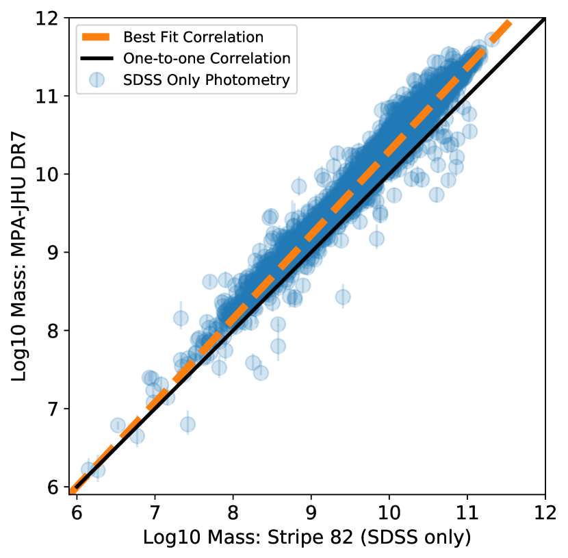
Figure 9: Comparison of kcorrect-derived Stripe 82 galaxy masses and the masses from the MPA-JHU sample originally presented in Kauffmann et al. (2003) with DR4 data and updated for DR7. The fit slope is 1.07 with offset -0.43 dex.

If we assume that the error in kcorrect can be estimated by the root-mean-square of the difference between kcorrect and MPA/JHU, then the error is $\sim 0.32$ dex. This error estimate is also consistent with the error determined in Rose et al. (2019). With this estimate of the mass error, we can confirm that our derived masses are systematically lower than those see in Kelly et al. (2010). But these differences are not significant on the scale of the mass range of the host galaxies, and most importantly, do not preferentially change the ordering of galaxies in mass.

3 Hubble Diagram

We here present the NIR and optical Hubble diagram from the current global collection of literature data on SNeIa observed in restframe $H$.

3.1 Lightcurves

We used the SNooPy fitter of Burns et al. (2011) to estimate maximum magnitudes in $H$ with the “max_model” for the collected sample of supernovae. We fit the optical lightcurves with the SNooPy “EBV_model2”. For both models, we use the parameterization based on the updated $s_{BV}$ width parameter introduced in Burns et al. (2014).

We adopted the same approach as in Weyant et al. (2014) of fitting separately in each band using the “max_model” SNooPy model. Unlike in Weyant et al. (2014), where we held $\Delta m_{15}=1.1$ fixed, we here fit for the width parameter $s_{BV}$. We first fit with the reported time of maximum B-band light, T${}_{B_{\rm max}}$, from the original spectroscopic confirmation announcement (generally ATel or CBET). For most of the SNeIa, we had constraining lightcurve information in the optical or NIR that started before peak brightness, we generated an updated T${}_{B_{\rm max}}$ from a lightcurve fit to all available data. We then recorded these updated T${}_{B_{\rm max}}$ values along with the original estimates for those not updated and ran the final lightcurve fits with T${}_{B_{\rm max}}$ fixed.

In total, there are 36 objects without optical or NIR observations before T${}_{B_{\rm max}}$; however, only 16 of these objects pass the cuts to be in either the NIR or optical Hubble diagrams. For these 16 SNeIa that had no optical or NIR lightcurve points before T${}_{B_{\rm max}}$, we used the spectroscopic original T${}_{B_{\rm max}}$. Two of them, PTF11qri and PTF13ddg, did have raw lightcurves of the transient as published by PTF DR3.^, These lightcurves did not include explicit host-galaxy subtraction and so are unreliable for determining accurate brightness, but the relative magnitudes of the lightcurves are useful to determine a time of T${}_{B_{\rm max}}$. We used these lightcurves to confirm that the time of maximum light from the optical photometry was consistent with the spectroscopic estimate.

The sample of SNeIa came from several surveys and the different transmission curves were accounted for in SNooPy using the corresponding CSP transmission curves, WHIRC transmission curves, and 2MASS (for PAIRITEL) transmission curves.

We used the default SNooPy $K$-corrections using the Hsiao et al. (2007) spectral templates, but we did not warp the spectral templates to match the observed color (“mangle=False”). We do not apply any color-luminosity correction as we do not assume a relationship between the different filters in our “max_model” fitting.

We did not use lightcurves that were observed before 1990, had no known optical T${}_{B_{\rm max}}$, or were known to be SN 1991bg-like or other peculiar types (although we include SN 1991T-like events). We excluded from the Hubble residual analysis any SN Ia that had fewer than three lightcurve points in the $H$-band. After these quality cuts, we have a sample of 144 SNeIa.

The lightcurve fits to SNe Ia presented here are shown in Figures 10–10.2. Errorbars are included on the plot but are smaller than the markers. We did not use non-detections in these fits.

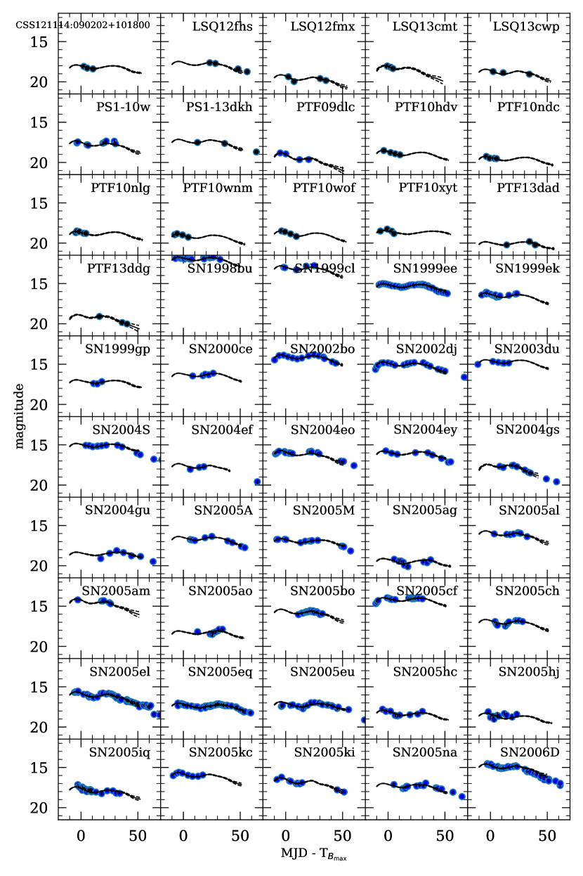
Figure 10: The SNooPy $H_{\rm max}$ lightcurve fits to 144 SNeIa. Error bars are smaller than the markers.

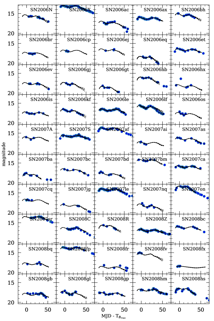
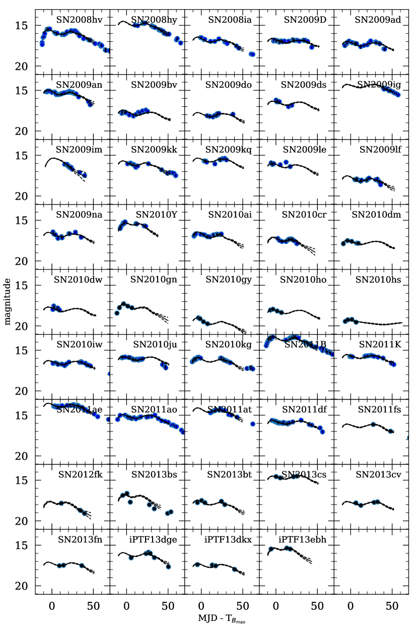
Figure 10.1: The SNooPy $H_{\rm max}$ lightcurve fits to 144 SNeIa. Error bars are smaller than the markers.

Figure 10.2: The SNooPy $H_{\rm max}$ lightcurve fits to 144 SNeIa. Error bars are smaller than the markers.

The $H$-band magnitudes are reported as the fit apparent magnitude based on the “max_model” template for the given $s_{BV}$. The SNooPy “max_model” templates are normalized to a magnitude of 0 at maximum light individually for each filter and for all values of $s_{BV}$. We apply no correction to the $H$-band apparent magnitude based on $s_{BV}$. For the optical fits, we do include the $s_{BV}$ correction to the apparent brightness through the default use of the SNooPy “EBV_model2” which includes the stretch-luminosity correction as part of the fit and estimation of distance modulus. The “max_model” and “EBV_model2” do not account explicitly for intrinsic color variations, but both models do remove Milky Way reddening (Schlafly & Finkbeiner, 2011). “EBV_model2” also accounts for host galaxy extinction using all of the optical filters by fitting for E(B-V) while holding $R_{V}$ constant. To emphasize this distinction we quote the $H$-band fits in terms of apparent magnitude and the optical fit results in terms of distance modulus ($\mu$).

3.2 Hubble Diagram

We compare our measured SN Ia apparent brightness to that predicted by a flat LCDM model with $H_{0}=72$ km s^-1 Mpc^-1 and $\Omega_{M}=0.28$ (Perlmutter et al., 1999; Freedman et al., 2001). We calculated the weighted best fit value of the absolute magnitude, after adding both an intrinsic dispersion of 0.08 mag (as reported in Barone-Nugent et al., 2012) and the equivalent magnitude uncertainty from a peculiar velocity of 300 km s^-1 in quadrature to the reported statistical fit uncertainty from SNooPy. We redid the full analysis at 150 km s^-1 and found minimal differences. These additions to the uncertainty were used in computing the weighted average, but are not included in the errors plotted on the residual plots or reported in Table 15. While SNooPy “max_model” reports apparent brightness and “EBV_model2” returns distance modulus, the actual calculation of residuals follows the same process. The absolute magnitude is entirely degenerate with the chosen value for $H_{0}$. As we are here looking at residual relative brightness, the absolute brightness and value of $H_{0}$ are not directly relevant. This model was then subtracted from the data points to yield the residuals that were used to compare against properties of the host galaxies.

The results from these fits are tabulated in Table 15 and the resulting Hubble diagram with residuals is shown in Figure 13.

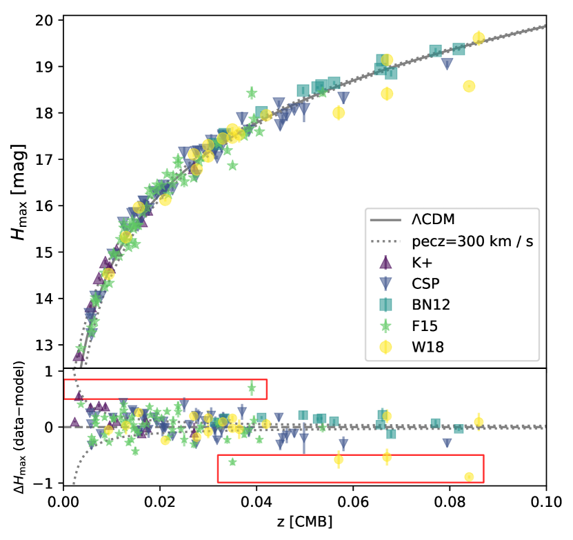
Figure 13: Top: SN Ia $H$-band Hubble diagram for the sample considered in this paper. Bottom: The residuals from the apparent $H$ magnitude at maximum light (data$-$model) for the best-fit $\Lambda$CDM cosmology. The points are coded in different shapes to indicate the source of the SN Ia lightcurve data. The 6 outliers referred to in Section 5.3 are highlighted in the red boxes. The additional intrinsic scatter (0.08 mag) and the error from peculiar velocities are not included in the error bars.

4 Analysis

In this section, we examine the host galaxy stellar mass correlations with the restframe $H$-band residuals and the optical width-luminosity-corrected distance modulus residuals. Though we present an in-depth study of host galaxy stellar mass since it is the largest trend seen in the literature with optical lightcurves, we have done the same studies examining restframe $K$-corrected absolute $r$-band magnitude as well as briefly exploring other properties of the supernova environment ($g-r$ color, Hubble flow, NUV colors, and distance from center of host galaxy). These studies are summarized in Appendix A.

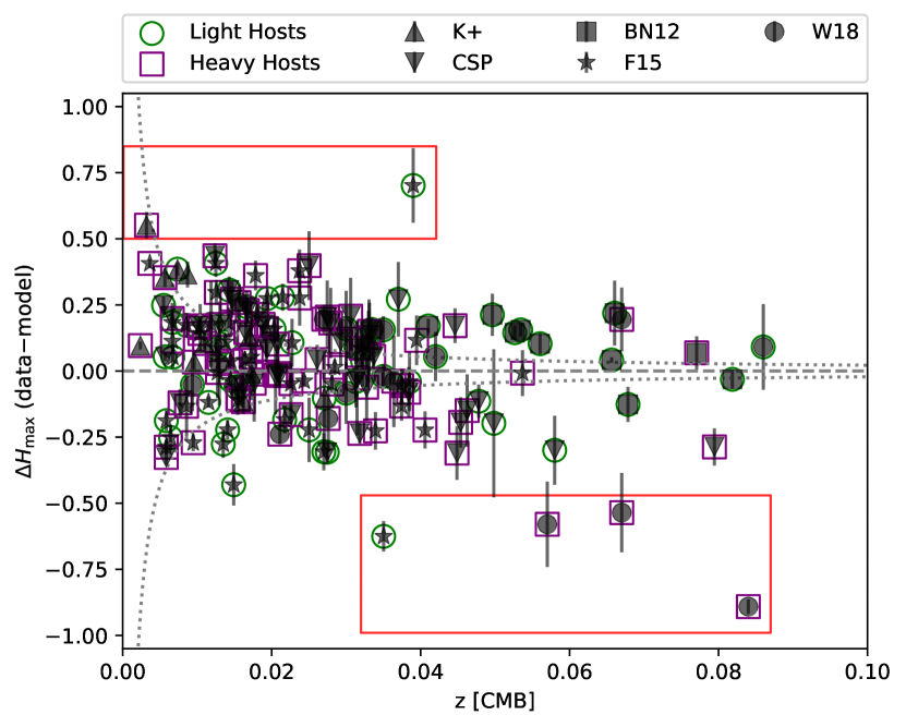
Figure 14: The residuals from the apparent $H$ magnitude at maximum light (data$-$model) for the best-fit $\Lambda$CDM cosmology. The points are coded in different shapes to indicate the source of the SN Ia lightcurve data. If no host galaxy mass was calculated, the point does not have a circle or square around it. Overlaid on the points are the classification of their host galaxy: green circles are galaxies with mass $<10^{10}M_{\odot}$ and purple squares are galaxies with mass $>10^{10}M_{\odot}$. The 6 outliers referred to in Section 5.3 are highlighted in the red boxes. The additional intrinsic scatter (0.08 mag) and the error from peculiar velocities are not included in the error bars.

4.1 Statistical Properties of the Distributions

Having collected UV, optical, and/or NIR data allows us to estimate stellar masses for 143 out of 144 host galaxies. We separate this sample by mass where the “Light” population corresponds to galaxies with masses less than $10^{10}~{}M_{\odot}$ and the “Heavy” population corresponds to galaxies with masses greater than $10^{10}~{}M_{\odot}$. Figure 14 shows the Hubble residuals as a function of redshift with Light and Heavy galaxies highlighted. Those with no indicator do not have sufficient host galaxy photometry to estimate mass. We observe a population of 4 bright (residual $<-0.5$ mag) SNeIa at $z>0.03$ plus 2 additional dim outlier (residuals $>0.5$ mag). We see no clear trend in host galaxy mass versus redshift.

The top left plot of Figure 15 shows the $H_{\rm max}$ Hubble residuals ($\Delta H_{\rm max}$) versus host galaxy mass and the top right plot shows a histogram of the Hubble residuals grouped by mass with the full sample included in grey for comparison. Table 4 shows the full details of the fits for the different populations including their peak residual magnitude, weighted peak residual magnitude, $\chi^{2}$, $\chi^{2}$/DoF, standard deviation, interquartile range (IQR), the standard error on the mean (SEM), and the intrinsic standard deviation that would result in a reduced $\chi^{2}=1$.

Figure 15: Top Left: SN Ia Hubble residuals vs host galaxy mass. The points are coded in different shapes to indicate the source of the SN Ia lightcurve data. Overlaid on the points are the classification of their host galaxy: green circles are galaxies with mass $<10^{10}M_{\odot}$ and purple squares are galaxies with mass $>10^{10}M_{\odot}$. Bottom Left: Same as top left but for the distance modulus from optical lightcurves. Top Right: Histogram of Hubble residuals (data$-$model) for the SNeIa of the full sample (grey dashdotted). The dotted vertical lines correspond to the weighted averages of the full (grey), light (green), and heavy (purple) samples. Bottom Right: Same as top right but for the distance modulus from optical lightcurves. The additional intrinsic scatter (0.08 mag) and the error from peculiar velocities are not included in the error bars.

We find that the measured unweighted standard deviation of the whole sample is 0.229 mag and the IQR equivalent to $1~{}\sigma$ assuming a Gaussian distribution is 0.207 mag. The standard deviation (IQR) of SN Ia residuals in Light hosts is 0.223 (0.208) mag, while the standard deviation (IQR) of SNeIa residuals in Heavy hosts is 0.231 (0.206) mag.

The weighted average residual of the Light population is 0.027 $\pm$ 0.029 mag and the weighted average residual of the Heavy population is -0.024 $\pm$ 0.025 mag. The difference in average weighted residuals is 0.051 $\pm$ 0.038 mag with more massive galaxies hosting brighter SNeIa, which is not a detection at 1.34-$\sigma$ but has an amplitude in agreement with the literature.

If we remove the outlier population at $|\Delta H_{\rm max}|\geq 0.5$ mag, the separation between the peaks drops to 0.002 $\pm$ 0.039 mag, a 0.005-$\sigma$ significance (Table 4) indicating these outliers are driving the $\sim 1$-$\sigma$ shift seen in the full sample. We will explore this “outlier population” further in Section 5.3.

Table 4: NIR SN Sample Mean and Std Deviations

Sample	SNeIa	residual	wgt residual	$\chi^{2}$	$\chi^{2}$/DoF	stddev	IQR	SEM	Implied $\sigma_{H}^{int}$	Notes
		$\mathrm{mag}$	$\mathrm{mag}$			mag	$\mathrm{mag}$	mag	$\mathrm{mag}$
All	144	0.031	-0.000	346.2	2.40	0.229	0.207	0.019	0.174
Light	59	0.032	0.027	125.2	2.12	0.223	0.208	0.029	0.171	$M<$ 1e+10 $M_{\odot}$
Heavy	84	0.026	-0.024	219.1	2.61	0.231	0.206	0.025	0.175	$M\geq$ 1e+10 $M_{\odot}$
Light	57	0.032	0.037	79.6	1.40	0.190	0.202	0.025	0.120	$M<$ 1e+10 $M_{\odot}$,
										$|\Delta H_{\rm max}|<0.5$ mag
Heavy	80	0.046	0.022	97.3	1.22	0.182	0.177	0.020	0.105	$M\geq$ 1e+10 $M_{\odot}$,
										$|\Delta H_{\rm max}|<0.5$ mag
Hubble Flow	80	-0.013	-0.028	282.0	3.53	0.236	0.214	0.026	0.208	$z>0.02$
Hubble Light	35	0.020	0.022	97.0	2.77	0.226	0.196	0.038	0.193	$z>0.02$, $M<$ 1e+10 $M_{\odot}$
Hubble Heavy	45	-0.038	-0.073	185.1	4.11	0.240	0.208	0.036	0.218	$z>0.02$, $M\geq$ 1e+10 $M_{\odot}$
Hubble Light	33	0.019	0.034	51.3	1.55	0.166	0.191	0.029	0.127	$z>0.02$, $M<$ 1e+10 $M_{\odot}$
										$|\Delta H_{\rm max}|<0.5$ mag
Hubble Heavy	42	0.007	-0.012	63.9	1.52	0.172	0.180	0.027	0.126	$z>0.02$, $M\geq$ 1e+10 $M_{\odot}$
										$|\Delta H_{\rm max}|<0.5$ mag

4.1.1 Correlations with Corresponding Optical Lightcurves

Host galaxy correlations have been well studied in the optical wavelengths. To compare our results to these studies, we repeated the analysis with optical lightcurves of SNeIa observed in the $H$-band. The optical data set is only 104 SNeIa in total and 103 with host galaxy mass estimates. The bottom panels in Figure 15 shows the distributions from host galaxy stellar mass compared with the optical distance modulus ($\mu$) residuals. Table 5 presents the resulting weighted residuals and standard deviations. Here we see no difference in the Light and Heavy host galaxies with a difference in average weighted residuals $0.058\pm 0.039$ mag, which is $\sim 1.5~{}\sigma$. The $\Delta H_{\rm max}$ outliers are not outliers in this sample and no objects have $|\Delta\mu|\geq 0.5$ mag.

Comparing the NIR and optical data sets, the NIR sample is $41\%$ low mass galaxies while the optical sample consists of only $32\%$ low mass host galaxies. The low mass galaxies are more represented in the NIR than in the optical, but from Figure 15 we can see that the low mass distributions have similar shapes. We used the Z-test statistic to compare how similar the NIR and optical low mass galaxy residual distributions were and found a value of 0.07, which corresponds to a p-value of 0.47, indicating they are from the same distribution. Though the low mass galaxies may be a smaller percentage of the total population, they are still representative of the full distribution.

In this histogram analysis, we found no statistically significant trends between restframe $H$ or optical SN Ia brightness and host galaxy mass.

Table 5: Optical SN Sample Mean and Std Deviations

Sample	SNeIa	residual	wgt residual	$\chi^{2}$	$\chi^{2}$/DoF	stddev	IQR	SEM	Implied $\sigma_{\mu}^{int}$	Notes
		$\mathrm{mag}$	$\mathrm{mag}$			mag	$\mathrm{mag}$	mag
All	104	0.022	-0.000	165.4	1.59	0.190	0.196	0.019	0.128
Light	33	0.057	0.039	52.5	1.59	0.185	0.168	0.032	0.132	$M<$ 1e+10 $M_{\odot}$
Heavy	70	-0.000	-0.019	110.1	1.57	0.185	0.171	0.022	0.124	$M\geq$ 1e+10 $M_{\odot}$
Hubble Flow	52	-0.009	-0.017	112.8	2.17	0.170	0.178	0.024	0.147	$z>0.02$
Hubble Light	15	0.052	0.033	36.4	2.43	0.183	0.160	0.047	0.165	$z>0.02$, $M<$ 1e+10 $M_{\odot}$
Hubble Heavy	37	-0.034	-0.038	76.3	2.06	0.158	0.157	0.026	0.140	$z>0.02$, $M\geq$ 1e+10 $M_{\odot}$

4.2 Functional Form of Correlation

In the previous section, we compared the weighted mean residuals of SNeIa separated by host galaxy mass. However, there is no strong reason to model any host-galaxy brightness dependence by a simple step function. To further test the significance of this correlation, we explore different function forms for to relationship between SN Ia Hubble diagram residuals and the host galaxy stellar mass.

4.2.1 Different Models to Fit

We fit 7 different models using scipy.optimize.curve$\_$fit: a constant function corresponding to a single population and no correlation, a linear function, a step function with a break corresponding to the threshold used in the previous section ($10^{10}M_{\odot}$), a step function that fits for the location of the break as well as the amplitude and y-intercept, and several logistic functions. We fit three logistic functions: one where the threshold was held constant at $10^{10}~{}M_{\odot}$, one where it was allowed to float, and the generalized logistic equation. The error on the fitted model parameters corresponds to the diagonal elements of the resulting covariance matrix.

After fitting the different functions to our data, we compare which model describes the data better using two different information criteria (ICs): the Akaike Information Criterion (AIC; Akaike, 1974) and the Bayesian/Schwartz Information Criterion (BIC; Schwarz, 1978). We use the updated AIC_c (Sugiura, 1978), which is more suitable for smaller samples.

Information criteria allow for a comparison of different models by balancing an improved $\chi^{2}$ versus an increase in the number of fit parameters. However, AIC_c and BIC cannot be used to determine the absolute goodness-of-fit of the model; they can only establish which model the data favor compared to another model. We calculate $\Delta$AIC_c and $\Delta$BIC relative to the constant model. If the difference in IC is $>2$, a constant model is preferred; $>5$, a constant model is strongly preferred; $<-2$, the compared model is preferred; and $<-5$ the compared model is strongly preferred. When $0<$ IC $<2$, there is a preference for a constant model, but not a statistically significant one. Likewise, an IC between $-2$ and $0$ shows a preference for the compared model, but it is not significant.

Figure 16: Results from finding the best fit step location and fitting several functions to the residuals versus host galaxy mass. Top: Best fit location of the step function threshold shown using the AIC_c. The grey band highlights the area that we consider for the step function break such that the lower or higher mass bin has at least $20\%$ of the total SNeIa. Bottom: Various functions fit to the host galaxy mass versus Hubble residuals. The blue, dashed line shows the best fit step function is the outliers are removed (Section 5.3). These plots do show the additional 0.08 mag intrinsic scatter that was introduced as a lower bound and the peculiar velocity errors. Left: Results from using the $H_{\rm max}$ Hubble residuals. Right: Results from using the distance modulus ($\mu$) optical lightcurve Hubble residuals. The additional intrinsic scatter (0.08 mag) and the error from peculiar velocities are included in the error bars for both $H_{\rm max}$ and $\mu$.

4.2.2 $H$-band and Optical Results

To estimate the best site of the break (step function) or midpoint (logistic function), we fixed the position at a range of values between $7<\log_{10}{({\rm mass}/M_{\odot})}<12$ and fit for the other parameters in the respective models. We then use the ICs to compare the model at each transition location versus the model with the step or midpoint located at the original threshold of $10^{10}~{}M_{\odot}$ and chose the location with the lowest IC. The top panels of Figure 16 show the results from doing this procedure for the step function for $\Delta H_{\rm max}$ and the optical distance modulus ($\Delta\mu$).

The top left panel is the result of fitting 143 $H_{\rm max}$ residuals and has a minimum at $10^{10.43}~{}M_{\odot}$. Below a mass of $10^{8.96}~{}M_{\odot}$, the lower mass bin has less than $20\%$ of the total number of SNeIa making it more susceptible to edge effects during fitting. The same is true for the higher mass bin above a mass of $10^{10.65}~{}M_{\odot}$. Therefore, we only consider breaks in the step function between $10^{8.96}~{}M_{\odot}$ and $10^{10.65}~{}M_{\odot}$, which is indicated in the grey band in the top panels in Figure 16. The top right panel finds the best fit location for the 103 optical lightcurves favors a threshold at $10^{10.65}~{}M_{\odot}$.

The ICs strongly prefer a break at $10^{10.43}~{}M_{\odot}$ over $10^{10}~{}M_{\odot}$ for $H_{\rm max}$ residuals but prefer a larger mass $10^{10.65}~{}M_{\odot}$ for the break in $\mu$ residuals. Both the $H_{\rm max}$ and $\mu$ residuals favor a mass step that is in between the typical number found at $10^{10}~{}M_{\odot}$ (e.g., Sullivan et al., 2010; Lampeitl et al., 2010; Gupta et al., 2011; Childress et al., 2013b) and $10^{10.8}~{}M_{\odot}$ found in Kelly et al. (2010).

The bottom panels of Figure 16 show the models from the best fits: constant, linear, and the best-fit step function. Table 6 summarizes the best fit models using ICs and Table 7 outlines the significance in the slope of the linear function, the step size of the best-fit step function, and the step size of the step function with a break at the original threshold. We recover a $2$-$\sigma$ detection of a small slope but the ICs do not have a significant preference for a linear or constant model ($-2<$ ICs $<2$). However, the AIC_c strongly prefers a step function at the best-fit break over a constant model while the BIC favors a step function without being conclusive. The best-fit step at $10^{10.43}~{}M_{\odot}$ finds a $0.13\pm 0.04$ mag step at $3.25~{}\sigma$.

Table 6: Information Criteria Results for Different Models

Residual	Fit	$\Delta$ AICc	$\Delta$ BIC
$H_{\rm max}$	Constant	0.00	0.00
	Linear	-1.68	1.23
	Step: 10.00	0.45	3.35
	Step: 10.43	-5.27	-0.51
	Modified Logistic: 10.65	0.62	9.25
	Modified Logistic: 10.00	0.41	6.19
	Generalized Logistic	10.59	24.81
$\mu$	Constant	0.00	0.00
	Linear	-5.22	-2.66
	Step: 10.00	-0.44	2.11
	Step: 10.65	-9.06	-3.99
	Modified Logistic: 10.65	-6.58	0.96
	Modified Logistic: 10.00	-3.75	1.32
	Generalized Logistic	10.84	23.17

Table 7: Significance of Linear and Step Function Fits

Residual	Fit	Constant	$\sigma_{\rm Constant}$	Slope${\rm|}$Step	$\sigma_{\rm Slope|Step}$	Units
$H_{\rm max}$	Constant	0.00	0.02			mag
	Linear	0.42	0.22	-0.04	0.02	mag (log $M_{\odot}$)-1
	Step: 10.00	0.03	0.03	-0.05	0.04	mag
	Step: 10.43	0.04	0.02	-0.13	0.04	mag
$\mu$	Constant	0.00	0.02			mag
	Linear	0.53	0.20	-0.05	0.03	mag (log $M_{\odot}$)-1
	Step: 10.00	0.04	0.04	-0.06	0.04	mag
	Step: 10.65	0.03	0.02	-0.14	0.04	mag

The ICs from distance modulus residuals favor a non-constant model more frequently than the $H_{\rm max}$ residuals. A linear correlation is found at a $1.67$-$\sigma$ significance level and the ICs favor/strongly favor a linear model over the constant model. The best-fit step function was found at a 3.5-$\sigma$ significance level and the ICs favor to strongly favor this model over the constant model. The best-fit step at $10^{10.65}~{}M_{\odot}$ finds a $0.14\pm 0.04$ mag step, but if we move the step to match the $H_{\rm max}$ residuals, the step size is reduced in size to $0.10\pm 0.03$ mag with similar significance. We do not measure a significant step at $10^{10}~{}M_{\odot}$ as found previously in the literature.

The modified logistic function provides a smooth transition between two populations unlike a step function which is an abrupt change; however, this model introduces an additional free parameter. For both residuals, the best fit midpoint is at the highest allowed mass. With the additional free parameter, the ICs more clearly favor a constant model with the AIC_c preferring no model and the BIC strongly preferring a constant function. No transition between populations was found when using a modified logistic function at the $10^{10}~{}M_{\odot}$ midpoint and the ICs prefer a constant model. Given the ICs favor the step function more when compared to a constant model, we do not show the curves in Figure 16 or include any of the fit parameters.

For the $H_{\rm max}$ and $\mu$ residuals, the generalized logistic function returned a straight line which completely overlaps with the constant model; however, the ICs do not prefer this model due to the additional parameters it introduced. Since the ICs were strongly against these models in every scenario, we do not include the fit on the plots or the fit parameters.

We showed here that there is evidence of a trend between host galaxy mass and the $H_{\rm max}$ NIR lightcurves in which more massive galaxies host SNeIa that are brighter than those hosted in lower mass galaxies by $0.13\pm 0.04$ mag. We also measured a trend between host galaxy mass and optical lightcurves in which more massive galaxies host SNeIa that have more negative width-luminosity corrected optical brightnesses by $0.14\pm 0.04$ mag. Our results also agree with the literature (Childress et al., 2013b) in that a step function is more preferred over a linear function to describe the correlation between residuals and host galaxy mass. Though we found some evidence for a trend, the information criteria failed to provide strong, conclusive support in $H_{\rm max}$ lightcurves. However, the ICs do enforce the trend measured with the optical lightcurves.

5 Discussion

In this section we will further explore the statistical significance of our analysis by studying the dependence on the number of pre-maximum lightcurve points, effects from using a heterogeneous set of SNeIa, the outlier population, modeling the underlying distribution with a Gaussian Mixture Model, joint data samples, the dependence on the location of the step, and finally whether we are adding new information by including the NIR. We also compare our result to U20 and discuss the physical interpretation of the results.

Figure 17: Left: SN Ia Hubble residuals vs the of number of lightcurve points before T${}_{B_{\rm max}}$. Right: Histogram of $H$-band residuals with 0 pre-max points in any band (grey dashed) and those with at least one pre-max point (blue, solid). There is no dependence of the residuals on the number of pre-maximum points. The brightest outlier, PTF13ddg, has no pre-maximum published lightcurve observations. It does, however, have unsubtracted photometry from the PTF lightcurve database that shows behavior consistent with its quoted T${}_{B_{\rm max}}$.

5.1 Residuals are Not Dependent on Number of Pre-Maximum Lightcurve Points

One reasonable concern is that the number of lightcurve points observed before T${}_{B_{\rm max}}$could affect the reliability of inferred maximum brightness. As discussed in Section 3.1, there were 14 SNeIa with no pre-maximum lightcurve points. Figure 17 shows that the Hubble diagram residuals were not dependent on the number of pre-maximum lightcurve points. We thus conclude that our brightness measurements are robust to the number of pre-maximum lightcurve points.

5.2 Comparison of Residuals per Sample

Here we look at the statistical properties of the residuals if we separate them per sample, which are summarized in Table 8. Figure 18 shows the $H_{\rm max}$ residuals colored by SN lightcurve source (Sample). The difference in weighted mean residuals between the brightest (W18) and dimmest (BN12) samples is 0.24 mag and 0.20 mag for the $H_{\rm max}$ and $\mu$ residuals, respectively (see Table 8). This difference between surveys is larger than any step size we see based on any host-galaxy feature. However, the brightest population comes from W18 which features 3 of the bright outlier SNeIa. These 3 SNeIa also factor into the larger standard deviation and intrinsic dispersion seen in W18. BN12, the dimmest sample, has the tightest standard deviation. We note that BN12 reported a small range in $B$-band stretch for their lightcurves indicating a data set lacking in intrinsic variation of SNeIa and 8 out of 9 BN12 SNeIa with host galaxy photometry are in blue galaxies.

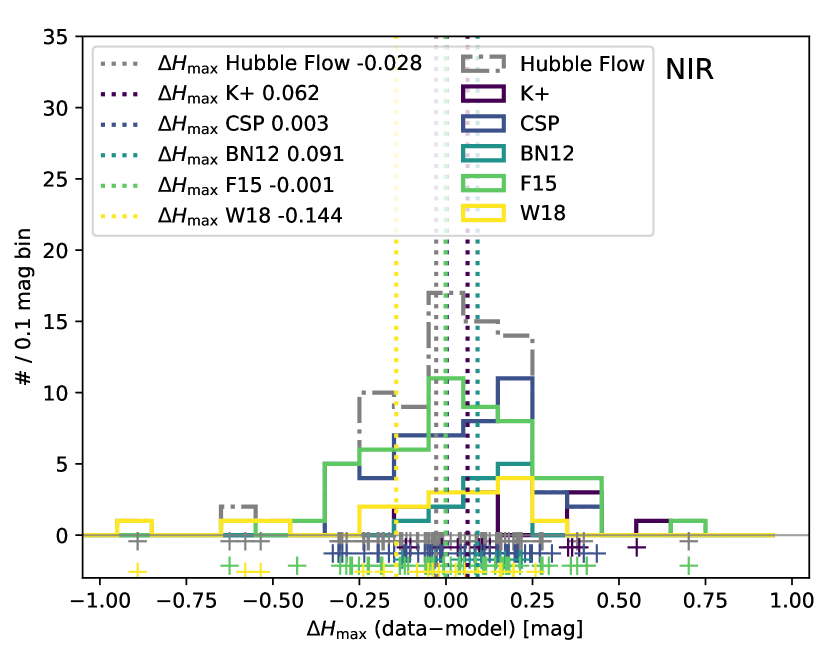
Figure 18: The $H$-band residuals for all Hubble flow SNeIa (grey dashed) and for each sample. The individual points are shown below the $y=0$ axis for ease of reference to the original data. The dotted vertical lines correspond to the weighted averages of the individual samples.

Table 8 has an additional column denoted “Step” which is the size and direction of the step function assuming a mass step break at $10^{10}M_{\odot}$. The $H_{\rm max}$ residuals per sample are all consistent with zero except the W18 sample. W18 contains most of the NIR outliers (Section 5.3). If these objects are removed, the size of the step, $-0.06\pm 0.09$ mag and $-0.08\pm 0.09$ mag for peculiar velocities of 300 km s^-1 and 150 km s^-1, respectively, is consistent with zero and the other samples. The $\mu$ residuals are more complicated with respect to the step. F15 shows $\sim 2$-$\sigma$ step inline with the literature. W18 exhibits a large, significant step that is not affected by the $H_{\rm max}$ outliers; however, there are only 8 objects in this sample and small number statistics is the likely driver of this result.

While the surveys have different mean properties in their residuals, they overall appear to form a continuous distribution. We thus assert that using SNeIa from different samples is not greatly biasing our results. A possible exception is BN12, which shows little variation in host galaxy type and may contain an intrinsically different distribution of SNeIa.

In Table 8, the K+ sample does not have a reported intrinsic dispersion for the $H_{\rm max}$ residuals. To determine the intrinsic dispersion, we set the $\chi^{2}$/DoF equal to one and solve for the intrinsic dispersion. For K+, this dispersion would have to be imaginary since the $\chi^{2}$/DoF is less than one. The K+ sample has a lower redshift distribution than the other surveys (see the purple triangles in Figure 13). The imaginary implied intrinsic dispersion is a manifestation of the high peculiar velocity choice of 300 km s^-1. The K+ sample is the lowest redshift collection (you can piece this out of Figure 13) and is thus most sensitive to the peculiar velocity assumed. If the assumed peculiar velocity is reduced to 150 km s^-1, the implied intrinsic dispersion for $H_{\rm max}$ residuals is $0.159$ mag. For all other surveys, the intrinsic dispersion changes by $\sim$-0.005$\pm$0.029 mag if the peculiar velocity is 150 km s^-1. We see a similar response to the change in peculiar velocities from the $\mu$ residuals. Though we do see small differences noted in Table 8, reducing the peculiar velocity has no affect on the outcome of this analysis.

The intrinsic dispersion assumed in the fitting analysis (0.08 mag) is clearly underestimating the intrinsic dispersion as reported in Table 8. We continue to use 0.08 mag as it represents a lower limit on what the intrinsic dispersion could be for a single, well-sampled survey. However, we reran the analysis while increasing the intrinsic dispersion to match the full sample implied $\sigma^{\rm int}$ from Table 8. For $\Delta H_{\rm max}$, the size of the step is reduced to $0.10\pm 0.04$ mag at $10^{10.43}M_{\odot}$, but $10^{10.43}M_{\odot}$ is still the location of the best fit step. The AIC_c is negative but favors no model and the BIC favors a constant model. The slope of the linear function is consistent with zero. For $\Delta\mu_{\rm max}$, the slope and step results from Table 7 are still valid but the ICs are reduced slightly. The step function at $10^{10.65}M_{\odot}$ is still strongly preferred over a constant model. Increasing the intrinsic dispersion degraded the step between host galaxy mass and $H$ residuals to 2.5-$\sigma$ but had no effect on the step for $\mu$ residuals.

Table 8: SN Sample Mean and Std Deviations - Surveys

Residual	Pec. Vel.	Sample	SNeIa	residual	wgt residual	$\chi^{2}$	$\chi^{2}$/DoF	stddev	IQR	SEM	Implied $\sigma^{\rm int}$	Step
	km s-1			$\mathrm{mag}$	$\mathrm{mag}$			mag	$\mathrm{mag}$	mag	mag	mag
$H_{\rm max}$	300	All	144	0.031	0.000	346.2	2.40	0.229	0.207	0.019	0.174	$-0.05\pm 0.04$
		K+	11	0.162	0.063	6.6	0.60	0.209	0.258	0.063	$\cdots$	$-0.01\pm 0.14$
		W18	18	-0.077	-0.144	135.6	7.53	0.301	0.219	0.071	0.291	$-0.36\pm 0.17$
		F15	56	0.022	-0.001	115.6	2.06	0.233	0.222	0.031	0.174	$0.05\pm 0.06$
		CSP	47	0.034	0.003	69.5	1.48	0.195	0.214	0.029	0.130	$0.06\pm 0.06$
		BN12	12	0.100	0.091	19.0	1.59	0.097	0.073	0.028	0.115	$-0.02\pm 0.11$
$H_{\rm max}$	150	All	144	0.017	0.000	474.0	3.29	0.229	0.207	0.019	0.197	$-0.03\pm 0.04$
		K+	11	0.148	0.080	18.0	1.64	0.209	0.258	0.063	0.159	$-0.13\pm 0.16$
		W18	18	-0.091	-0.131	153.4	8.52	0.301	0.219	0.071	0.297	$-0.30\pm 0.17$
		F15	56	0.008	-0.008	180.4	3.22	0.233	0.222	0.031	0.203	$0.05\pm 0.06$
		CSP	47	0.020	0.007	103.3	2.20	0.195	0.214	0.029	0.160	$0.04\pm 0.07$
		BN12	12	0.086	0.081	19.0	1.59	0.097	0.073	0.028	0.110	$-0.03\pm 0.11$
$\mu$	300	All	104	0.022	0.000	165.4	1.59	0.190	0.196	0.019	0.128	$-0.05\pm 0.06$
		K+	11	0.157	0.050	11.1	1.01	0.205	0.251	0.062	0.082	$0.17\pm 0.12$
		W18	8	-0.157	-0.091	23.7	2.96	0.201	0.165	0.071	0.214	$-0.39\pm 0.09$
		F15	39	0.048	0.042	54.4	1.40	0.171	0.162	0.027	0.118	$-0.10\pm 0.05$
		CSP	44	-0.006	-0.024	74.1	1.68	0.173	0.157	0.026	0.126	$0.05\pm 0.06$
		BN12	2	0.112	0.109	2.1	1.06	0.013	0.010	0.009	0.084	$\cdots$
$\mu$	150	All	104	0.012	-0.000	292.0	2.81	0.190	0.196	0.019	0.165	$-0.06\pm 0.04$
		K+	11	0.147	0.061	25.0	2.28	0.205	0.251	0.062	0.182	$0.11\pm 0.13$
		W18	8	-0.167	-0.128	39.4	4.92	0.201	0.165	0.071	0.245	$-0.34\pm 0.11$
		F15	39	0.038	0.041	102.4	2.63	0.171	0.162	0.027	0.157	$-0.11\pm 0.06$
		CSP	44	-0.016	-0.023	123.1	2.80	0.173	0.157	0.026	0.155	$0.06\pm 0.06$
		BN12	2	0.103	0.100	2.1	1.05	0.013	0.010	0.009	0.083	$\cdots$

5.3 Impact of the NIR Outlier Population

Out of 144 SNeIa there are 6 SNeIa with $|\Delta H_{\rm max}|>0.5$ mag as listed in Table 9. The four bright outliers SNeIa are LSQ13cmt, LSQ13cwp, PTF13ddg, and SN 2005eu. The two faint outliers are SN 1999cl and SN 2008fr.

Table 9: Outlier SNeIa

SN	Sample	$z$	$\sigma_{{\rm out},H}$	$\Delta H_{\rm max}$	$\Delta\mu$	$s_{BV,H}$	$N_{H}$	Phot	Profile	Mass	$g-r$	$M_{r}$	PGCD
				mag	mag					log${}_{10}(M_{\odot})$	mag	mag	Mpc
LSQ13cmt	W18	0.057	2.49	-0.57	–	0.68	3	DT	DeV	11.27	0.81	-23.56	0.0383
LSQ13cwp	W18	0.067	2.31	-0.53	-0.32	0.91	3	DT	DeV	11.00	0.78	-22.87	0.0153
PTF13ddg	W18	0.084	3.84	-0.88	–	0.70	3	ST	DeV	10.47	0.72	-21.50	0.0728
SN 2005eu	F15	0.035	2.71	-0.62	–	1.11	23	D	REX	9.02	0.49	-18.71	0.0009
SN 2008fr	F15	0.039	3.05	0.70	-0.00	1.10	6	S	DeV	7.90	0.38	-17.11	0.0008
SN 1999cl	K+	0.003	2.40	0.55	0.40	0.93	5	KT	EXP	10.55	–	–	0.0034

We excluded the 6 outliers and repeated the $\Delta H_{\rm max}$ fits versus host galaxy mass from Section 4.2. Table 10 presents the number of supernovae, the step size, and the best fit (BF) step location for the original sample and for the sample without the large outliers. The size of the step drops from $0.13\pm 0.04$ mag to $0.08\pm 0.04$ mag and the location of the best-fit step moved to $10^{10.64}M_{\odot}$, which is more similar to the optical residuals’ mass split location. The step function with outliers and without the outliers is directly comparable in Figure 16. The slope from the linear model was consistent with zero. All of the ICs either favor no model or the constant model.

3 out of 6 outlier SNeIa were also present in the optical data set with host galaxy mass, but none are also an outlier in that sample. The size of the step decreased by 0.01 mag which is a $3$-$\sigma$ detection and the best fit break stays the same, see Table 10. The ICs are now more conflicted with the the step function at $10^{10.65}M_{\odot}$ being strongly preferred by the AIC_c but the BIC has no model preference.

In the NIR, removing these large $H$-band outliers reduced the significance of the step reported above to $2$-$\sigma$ and moves the location of the step to $10^{10.65}~{}M_{\odot}$, which is the edge of the allowed range. The global minimum is closer to $10^{10.8}~{}M_{\odot}$ where there are fewer objects. The correlation is no longer partially preferred by the ICs over a constant model. If we force the step to be at $10^{10.43}~{}M_{\odot}$, the step size is $0.06\pm 0.03$ mag and the ICs do not prefer a step function over a constant model ($\Delta$ AIC_c=-1.53, $\Delta$ BIC=1.33). Part of the trend in the NIR was driven by the outlier population, mostly at $\Delta H_{\rm max}\leq-0.5$ mag, but a $2$-$\sigma$ detection still remains.

The outlier population impacts but does not fully determine the correlation of brighter SNeIa in more massive galaxies.

Table 10: Number of SNeIa for Different Sections

Section	Type	# $H_{\rm max}$	Step $H_{\rm max}$	BF Step Loc $H_{\rm max}$	AICc	BIC	# $\mu$	Step $\mu$	BF Step Loc $\mu$	AICc	BIC
			mag	log10 $M_{\odot}$			mag	log10 $M_{\odot}$
4.2.2	Original	143	$0.13\pm 0.04$	$10.43$	-5.3	-0.5	103	$0.14\pm 0.04$	$10.65$	-9.1	-4.0
5.3	No Outlier	137	$0.08\pm 0.04$	$10.64$	-0.3	5.4	100	$0.13\pm 0.04$	$10.65$	-6.5	-1.5
5.5	Joint	99	$0.12\pm 0.06$	$9.22$	0.1	5.0	99	$0.12\pm 0.04$	$10.55$	-7.4	-2.5

Note. — The ICs are relative to a constant model.

5.3.1 A Closer Look at the Outlier Population

We examined each outlier lightcurve more closely and found nothing unusual for LSQ13cmt or SN 2005eu. Though LSQ13cwp helped to discover a lensed galaxy system due to its proximity to it, this supernova is removed enough from the system to not be affected by the lens (Galbany et al., 2018a). PTF13ddg is notable because it is the largest outlier but it is at a redshift of 0.084 and only has 3 data points in the $H$-band. SN 2005eu from F15 has 23 lightcurve points in the $H$-band while the W18 SNeIa all have only 3 data points per lightcurve.

There are also two dim outliers. SN 1999cl is at a very low redshift of 0.003. While it is $>0.5$ mag dimmer, its significantly greater uncertainty from peculiar velocity makes it a non-significant outlier. The other dim outlier, SN 2008fr, is notable because it has no pre-max optical data (See Figure 17) – but it does have good sampling after T${}_{B_{\rm max}}$ such that we are confident that its time of maximum is reasonably accurate.

The W18 outlier population are located far from the center of the galaxy when compared to the bulk of the sample, see Figure 19. The median projected galactocentric distance (PGCD) for our full sample is $\sim 0.006$ Mpc and these SNeIa have values $0.015-0.073$ Mpc. The outliers from F15 and K+ are much closer to their host galaxies. The one feature (other than $z>0.03$) that is common amongst the 5 outliers not from peculiar velocities is that they are all in elliptical-like galaxies. The W18 outliers are from red ellipticals while the F15 galaxies are from small, blue, and round galaxies.

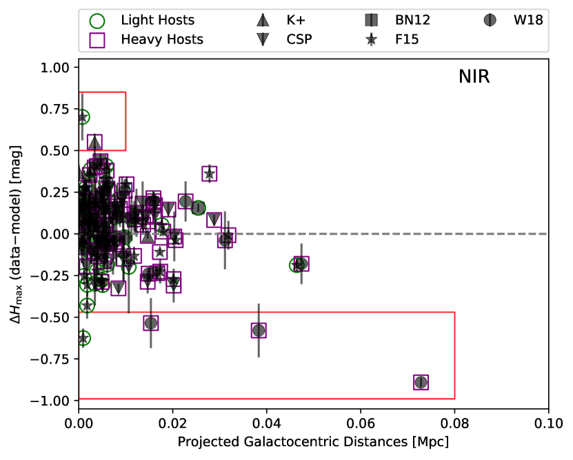
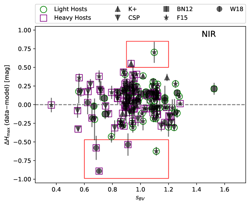
Figure 19: Left: SN Ia Hubble residuals vs projected galactocentric distances between the supernova and its host galaxy. Right: SN Ia Hubble residuals vs $s_{BV}$ stretch factor. For both figures, the points are coded in different shapes to indicate the source of the SN Ia lightcurve data. Overlaid on the points are the classification of their host galaxy: green circles are galaxies with mass $<10^{10}M_{\odot}$ and purple squares are galaxies with mass $>10^{10}M_{\odot}$. The six outliers referred to in Section 5.3 are highlighted in the red boxes. The additional intrinsic scatter (0.08 mag) and the error from peculiar velocities are not included in the error bars.

The right side of Figure 19 presents the distribution of the $s_{BV}$ values for the $H_{\rm max}$ model. These objects fall well within the distribution of the wider sample.

The column $\sigma_{{\rm out},H}$ in Table 9 presents how many sigma outside of the distribution these objects are. Only PTF13ddg and SN 2008fr are more than $3$-$\sigma$ outliers but all objects are within $4$ $\sigma$ of the distribution. For any cosmological-based analysis with this data set, we suggest removing this outlier population based on its large Hubble residual, but it is unclear that these are true outliers and not statistical fluctuations.

5.4 Gaussian Mixture Model

If a step function is an appropriate parameterization of the residual data, then a Gaussian Mixture Model (GMM) with two subpopulations should model the underlying distribution. Ponder et al. (2016) fit a GMM model assuming an evolution in the relative weights of two populations as a function of redshift. Here, we similarly fit for an evolution in population as function of host galaxy mass.

The scipy.optimize.curve$\_$fit function used for the different parameterizations cannot handle fitting for GMM parameters. Instead, we implemented the GMM likelihood in a Stan (Carpenter et al., 2017) model using PyStan (Riddell et al., 2018) which creates the full posterior distribution using a Hamiltonian Monte Carlo method. We fit a GMM with a mass evolution and without a mass evolution for the full sample and with the outliers removed. For the GMM with evolution, we normalized the $\log_{10}$ mass data by subtracting the mean and dividing by the standard deviation so that the fits were more stable. To compare how well this model performed, we used the AIC_c and BIC where the comparison is made to a single Gaussian model, which we took as the mean and standard deviation results from Tables 4 and 5.

Table 11: Information Criteria Results for Gaussian Mixture Models versus Single Gaussian Models

Residual	Fit	$\Delta$ AICc	$\Delta$ BIC
$H_{\rm max}$	Single Gaussian	0.00	0.00
	GMM	-4.75	-13.02
	GMM: No Evolution	-7.27	-15.54
	GMM: No Outliers	-2.16	14.96
	GMM: No Outliers/Evolution	-4.65	12.47
$\mu$	Single Gaussian	0.00	0.00
	GMM	1.58	13.97
	GMM: No Evolution	-0.57	11.82
	GMM: No Outliers	-6.64	4.26
	GMM: No Outliers/Evolution	-8.49	2.41

Table 12: GMM Fits

Residual	Fit	MeanA	$\sigma_{\rm intrinsic,A}$	MeanB	$\sigma_{\rm intrinsic,B}$	wA/slope	intercept
$H_{\rm max}$	GMM	-0.187	0.313	0.054	0.087	0.001	0.217
	GMM: No Evolution	-0.110	0.272	0.062	0.052	0.304
	GMM: No Outliers	-0.055	0.080	0.086	0.050	0.023	0.435
	GMM: No Outliers/Evolution	-0.054	0.079	0.089	0.043	0.437
$\mu$	GMM	-0.054	0.062	0.125	0.190	0.084	0.629
	GMM: No Evolution	-0.054	0.065	0.082	0.100	0.532
	GMM: No Outliers	-0.051	0.057	0.133	0.086	0.085	0.639
	GMM: No Outliers/Evolution	-0.051	0.060	0.089	0.098	0.537

The PDFs of the results of these fits can be examined in Figure 20 with the IC information is in Table 11 and the parameter values given in Table 12. The GMM with $H_{\rm max}$ is finding a second population mostly driven by the bright outliers. The ICs strongly favor a GMM with the outliers but are split between a single Gaussian model and GMM once they are removed. The $\mu$ residuals strongly favor a single Gaussian model with the outliers, but have some preference for a GMM once they are removed.

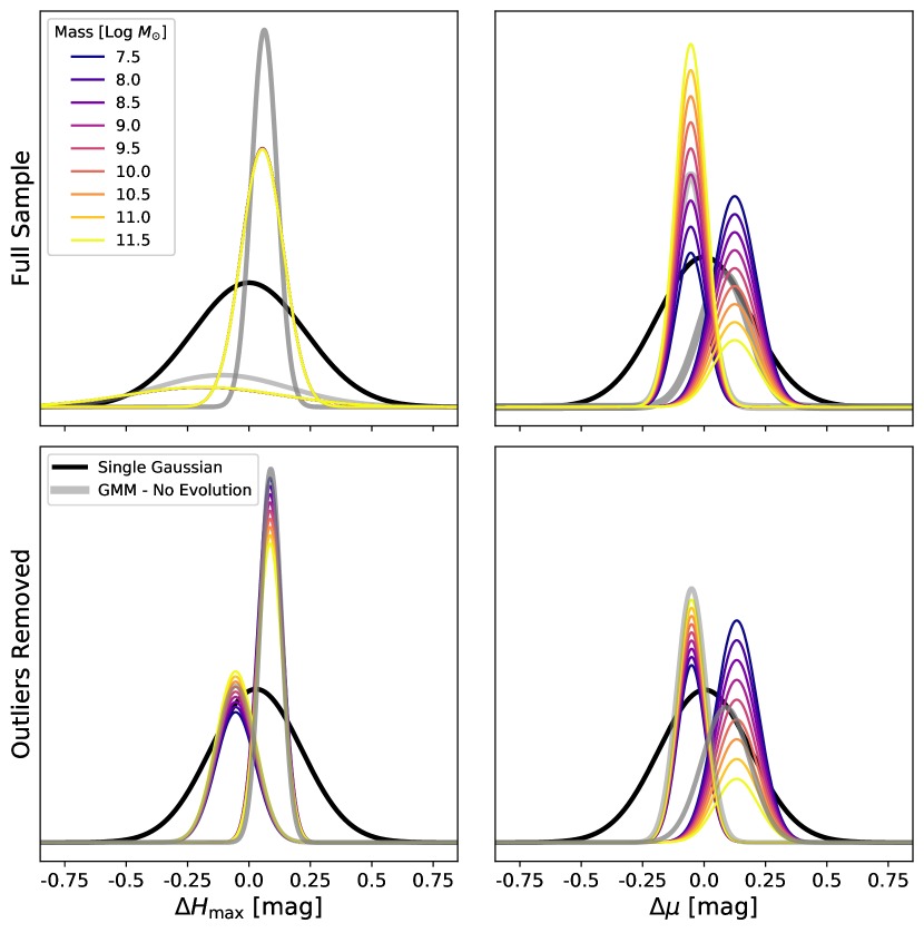
Figure 20: Fits of different Gaussian Mixture Models (GMMs) to $H$-band residuals (Left) and the optical residuals (Right) for the full samples (Top) and with the $H_{\rm max}$ outliers removed (Bottom). The multi-colored curves correspond to a GMM that evolves as a function of host galaxy mass. The grey curves are a GMM with no evolution and the black curves is a single Gaussian fit to the data.

The slope of the evolving GMM is larger for $\Delta\mu$ residuals than $H_{\rm max}$ indicating that the optical residuals may be more sensitive to changes in host galaxy mass.

A non-evolving GMM is more favored in the ICs than the evolving GMM partially because there is one less parameter to fit. Typically, the evolving GMM yields a larger difference in means except for $H_{\rm max}$ without outliers.

The bright $H_{\rm max}$ outliers are partially driving two populations in the $H$-band data but the optical data favors a GMM more when they are removed.

5.5 SNeIa with Both $H$-band and Optical Lightcurves

We here explore the results from limiting the data set to only the SNeIa that have both $H$-band and optical lightcurves. A summary of the results is presented in Table 10 under “Joint”.

99 SNeIa with host galaxy stellar masses measured have both NIR and optical lightcurves that satisfy our quality cuts for inclusion in the Hubble analysis. The $H$-band brightness residuals favor a step function at $10^{9.22}M_{\odot}$ with a decreased step of $0.12\pm 0.06$ mag and the BIC strong prefers a constant model while the AIC_c prefers no model. If we measure the step at $10^{10.43}M_{\odot}$, it is reduced to $0.07\pm 0.04$ mag. The optical correlation step size decreased by 0.02 mag but the location of the step moved to $10^{10.55}M_{\odot}$. The ICs are equivalent to those for the full sample. If we hold the step at $10^{10.65}M_{\odot}$, the step size is $0.07\pm 0.04$ mag.

The joint sample produced very different best fit step locations but neither had a strong preference with the ICs. If we measure both the optical and NIR step at the best fit location for the full sample, they both produce the same step amplitude at a $\sim 2$-$\sigma$ correlation.

5.6 Importance of the Location of the Step

To explore what is happening at low and high mass, we fit a constant model excluding the $\pm 0.2$ dex region surrounding the best fit break of $10^{10.43}M_{\odot}$. The constant fit model is consistent with the weighted average. Figure 21 shows the results of this fit with the best fit step function for the full sample as reference. The data in Figure 21 is binned with evenly distributed number of objects. It is easier to see the evolution and offsets between high and low mass in this reduced form. The difference between the low and high mass samples is $0.09\pm 0.05$ mag for $H_{\rm max}$ and $0.11\pm 0.05$ mag for $\mu$. Without the outliers, we measure a difference between the two is $0.07\pm 0.04$ mag for $H_{\rm max}$ and $0.10\pm 0.05$ mag for $\mu$.

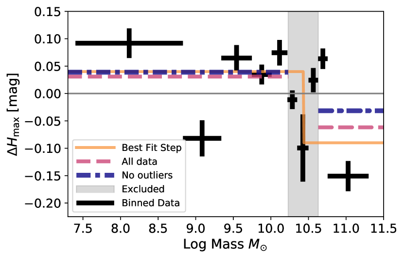
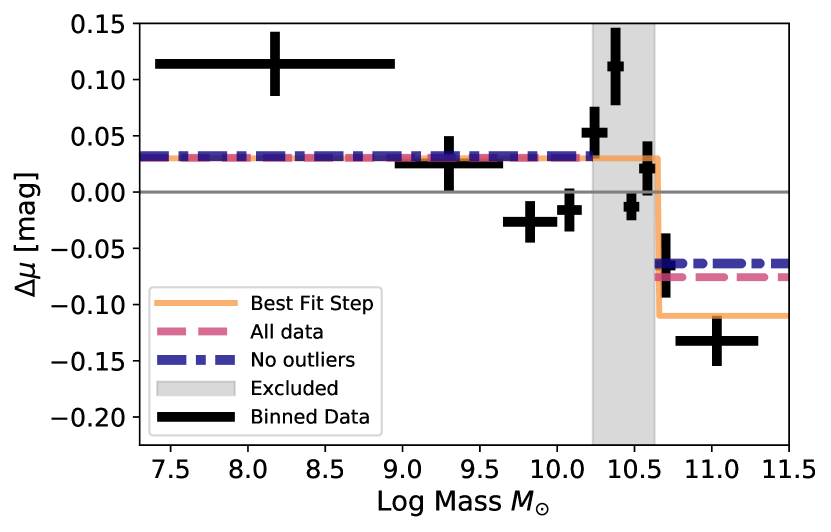
Figure 21: Left: The $H$-band residuals in 10 mass bins where the three lowest bins have 15 objects and the rest have 14 objects. The highest bin has a large offset from the others. The best fit break is at 10.43 log Mass $M_{\odot}$. The orange solid line is the best fit step function from Figure 16. The greyed area is the $\pm~{}0.2$ dex surrounded that break. The pink dashed line are the fits to the low and high mass objects on either side of the excluded area. The blue dash dotted line is the same as the pink line but with the outliers removed. The difference in the high and low mass fits are 0.09 mag and 0.07 mag for the full sample and the sample without outliers, respectively. Right: Same as left except for the $\mu$ residuals in 10 mass bins where the three lowest bins have 11 objects and the rest have 10 objects. The different in the high and low mass fits are 0.10 mag and 0.10 mag for the full sample and the sample without outliers, respectively.

5.7 Location of the Step Compared to Other Analyses

The best fit step locations ($10^{10.43}M_{\odot}$/$10^{10.65}M_{\odot}$) are higher than typically reported in other analyses. Since the masses here may be underestimated by 0.3 dex, the mass values are closer to $10^{11}M_{\odot}$. We examined 13 of the papers measuring a host galaxy mass step in the last 10 years and found that the majority of them assigned the value of $10^{10}M_{\odot}$ because it was used in Sullivan et al. (2010). Sullivan et al. (2010) used $10^{10}M_{\odot}$ because it was the median of the sample; however, they did also fit for a step function at $10^{10.5}M_{\odot}$ and found a $\sim 4$-$\sigma$ step. If an analysis did not use $10^{10}M_{\odot}$, then they used the median of their own sample which was typically much larger than $10^{10}M_{\odot}$ ($10^{10.5}M_{\odot}$-$10^{10.8}M_{\odot}$). It is of note that Sullivan et al. (2010) has the highest median redshift (0.65) of all the analyses which typically have a median redshift $\sim 0.03$ or $\sim 0.3$.

In summary, literature analyses either use the median of their host galaxy mass sample or use the break location from Sullivan et al. (2010); however, we fit for the location that maximized the size of the step. We leave the discussion of what should be the best location for a break to future analyses.

5.8 Are the NIR Residuals Adding More Information to the Optical Residuals?

Is the NIR analysis an independent test of host galaxy correlations or degenerate with the tests done at optical wavelengths? Figure 22 presents the $H_{\rm max}$ residuals plotted against the $\mu$ residuals for the 99 supernovae that have both NIR and optical data.

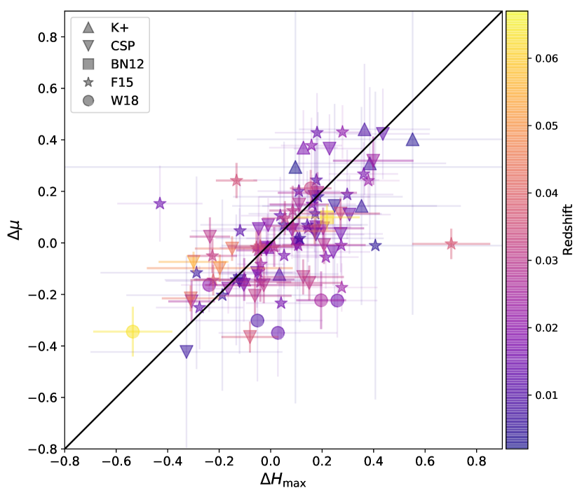
Figure 22: Optical Hubble residuals ($\mu$) vs. $H_{\rm max}$ residuals. The errors from peculiar velocities are included in the error bars for both $H_{\rm max}$ and $\mu$ but not the additional intrinsic scatter (0.08 mag). All objects in the smooth Hubble flow have thicker and less transparent error bars to improve readability. As in previous figures, the different shapes indicate the source of the SN Ia lightcurve data. The color map indicates the redshift of the host galaxy. The black line illustrates a one-to-one relationship to guide the eye. The Pearson r-coefficient is 0.59.

One source of potential correlation is a mis-estimate of the cosmological redshift for a supernova. If we use the wrong cosmological redshift for an object, we would expect to see strong correlations between the optical and NIR brightnesses due to using the wrong cosmological redshift rather than due to any intrinsic physics about the supernova. In particular, the lower redshift supernovae ($z<0.02$) are affected by larger peculiar velocities. In Table 13, we present the mean, weighted mean, standard error on the mean, standard deviation and Pearson correlation coefficient ($r$) for the full sample and if the sample was split at $z=0.02$. The samples of $z<0.02$ and $>0.02$ have offset weighted means but they are within $2~{}\sigma$ of each other. Both samples have a strong correlation between optical and NIR supernovae indicating that peculiar velocities are not a driving their correlation.

The optical and $H$ Hubble residuals are clearly and strongly correlated. This is not a surprise as effectively similar relationships are found when considering large sets of lightcurves in training lightcurve fitters. But we here we have answered the question from a data-driven exploration with Hubble residuals directly from a significant selection of supernovae not involved in the construction of the SNooPy templates.

Table 13: Optical - $H$ Hubble Residuals

Sample	# SNeIa	Mean	Wgt Mean	SEM	Std. Dev.	Pearson’s $r$
		mag	mag	mag	mag
All	99	0.05	0.02	0.02	0.19	0.59
$z<0.02$	51	0.06	0.06	0.03	0.18	0.61
$z>0.02$	48	0.04	0.00	0.03	0.18	0.54

5.9 Comparison to the Carnegie Supernova Project

We measured a $3.25$-$\sigma$ correlation between $H_{\rm max}$ residuals and host galaxy mass which dropped to $2$-$\sigma$ (at the best-fit step break) when removing the outliers. These results are in agreement with U20. A key difference between the CSP sample and our sample is that U20 had substantially fewer lower-mass galaxies, see Figure 23. U20 used the “max_model” fitting for the optical and NIR filters such that we can directly compare our $H_{\rm max}$ residuals but not the $\mu$ residuals since each optical filter was fit independently. A constant location of the break for the step function was used in U20 which was the median of the sample at $10^{10.48}M_{\odot}$. In contrast, the median of the sample in this paper is $10^{10.20}M_{\odot}$, but our models favor a step at a mass closer to the median from CSP. We compared our results their “All” sample and find their $H$-band step magnitude in agreement with any of our subsamples. Furthermore, examining all the optical filters, their measured step has an amplitude ranging from 0.147 mag to 0.074 mag with the trend ranging from 2.5 to $3.3~{}\sigma$. This agrees with the recovered step magnitude for $\mu$ in this paper.

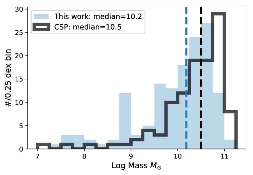
Figure 23: Mass distribution of this work compared to that of Uddin et al. (2020). This work has more lower-mass objects

5.10 Direction of the $H$ versus Optical Correlation

The trend we observed in the $H$-band peak magnitudes is that larger galaxies, which are also more red and more likely to be ellipticals, host brighter supernova than lower mass galaxies, which are bluer and more likely spirals. This correlation is the opposite of the trend observed in uncorrected optical brightness. Hamuy et al. (1995) first found that galaxies with a younger stellar population hosted brighter supernova. Continued works such as Hamuy et al. (1996) and Sullivan et al. (2006) found correlations with the lightcurve shape parameters $\Delta m_{B}$ and stretch $s$, respectively, where faster declining (dimmer) SNeIa were hosted in elliptical and higher-mass galaxies whereas slower declining (brighter) SNeIa were hosted in spiral and lower-mass galaxies. All subsequent analyses have found a correlation between host galaxy properties and the shape of the width of the lightcurve. However, after width-luminosity standardization, the correlation with host galaxy properties for optical SNeIa switches such that larger mass galaxies have brighter residuals than lower mass galaxies.

5.11 Physical Interpretation

We interpret the results above as an indication that more massive galaxies host SNeIa that are brighter in the NIR than those hosted in less massive host galaxies. This result is not strongly supported by all of the statistical tests implemented but it is supported at a $2$-$\sigma$ level. Our interpretation of the data here is in agreement with the results from the U20 paper which is not affected by potential biases from multiple SNeIa surveys.

Brout & Scolnic (2020) claim that the host galaxy stellar mass dependence seen at optical wavelengths is due to the correlation of dust in different galaxies. Because NIR is less sensitive to dust, we should not see any significant correlations between the NIR residuals and host galaxy mass if the correlation is driven by dust. This analysis has found some evidence to support a correlation between the NIR and host galaxy stellar mass; however, the trend is only seen at a $2$-$\sigma$ level. Therefore; we cannot conclude if the correlation is driven by dust alone.

5.12 A Caveat on K-Corrections

We note that the state of K-corrections in NIR SNeIa photometry remains in its beginning stages and we express concern that the K-corrections used here are not the final word. The two significant previously explicitly published K-corrections are those of Krisciunas et al. (2004b) and Hsiao et al. (2007). The community has continued to gather NIR spectra, but these have not yet been compiled into a new set of spectral templates. Stanishev et al. (2018) presented their own K-correction methodology, but do not provide an updated set of spectral templates. If SNeIa were all the same in the NIR, then the excellent NIR spectral series on SN 2011fe (Hsiao et al., 2013) or SN 2014J (Marion et al., 2015) would provide sufficient data for good K-corrections. But while SNeIa NIR exhibit less scatter in the $H$-band than the optical, there is still clear evidence for some variation: single- vs. double-hump (e.g., the dromedarian SN 2005hk detailed in Phillips et al., 2007), and bridge objects such as iPTF13ebh (Hsiao et al., 2015). We remain of the opinion that a new effort in K-corrections for SNeIa in the NIR would be a worthwhile endeavor with a clear benefit to the community.

6 Conclusion

We have collected and analyzed a data sample of 220 SNeIa with observations in the restframe $H$-band. We fit the lightcurves using SNooPy, and found 144 of the SNeIa had lightcurve fits suitable for inclusion in a Hubble diagram. We combined measurements from SDSS, DECaLS, PS1, 2MASS, and GALEX to determine photometric stellar masses for the host galaxies of 143 of these 144 SNeIa.

We explored possible correlations between $H_{\rm max}$ residuals from the SNooPy fitter and host galaxy properties. Though we only presented the results from host galaxy stellar mass in the main text, further studies are presented in Appendix A. Using the 143 SNeIa with host galaxy stellar mass measurements, we report a $0.13\pm 0.04$ mag step at $10^{10.43}M_{\odot}$ in agreement with the step seen at optical wavelengths. However, the AIC_c and BIC only mildly prefer this step function over a constant model. By further investigating the sample, we have shown that the correlation with $H$-band brightnesses is partially driven by outliers and removing these from the sample lowers the significance of the step to $2~{}\sigma$ at $10^{10.64}M_{\odot}$, but the ICs mildly prefer a constant model. We showed that a GMM is strongly favored compared to a single Gaussian when the outlier population is present, but the ICs are split with them removed.

The apparent outlier population of SNeIa in the $H$-band is located within the smooth Hubble flow ($0.03<z<0.09$) except for one dim, low redshift object whose residual is within peculiar velocity uncertainties. The set of 3 bright outliers from the W18 sample have a residual brightness $\leq-0.5$ mag after correction and are hosted in massive ($M>10^{10}M_{\odot}$), bright ($M_{r}>-21.5$ mag), and red ($0.6<g-r<0.8$ mag), elliptical galaxies. However, the host galaxy for the bright outlier SN 2005eu is a low mass, dim, and blue galaxy but it is small in angular size and possibly an elliptical galaxy. SN 2008fr is similarly located in a low mass, dim, and blue galaxy but it is dimmer than expected unlike the other outliers. These objects are not $5$-$\sigma$ outliers but without a clear reason for their large offsets, they should not be used for a cosmological analysis.

Using the optical lightcurves corresponding to the sample of NIR lightcurves, we measured a host galaxy mass step of $\sim$0.1 mag around $10^{10.43}M_{\odot}$ and 0.14 mag at the best fit step of $10^{10.65}M_{\odot}$. This measurement not affected by the removal of the corresponding $H$-band outliers. Interestingly, a GMM is more preferred in the optical once the outliers have been removed. Since the ICs are split in preference between the GMM and single Gaussian, we cannot make a definitive conclusion. Showing this trend using a third lightcurve fitter provides further evidence of either a physical phenomenon or that there is some intrinsic property that is not well understood in optical wavelengths.

The correlation found between $H$-band residuals and host galaxy mass is the opposite correlation seen with optical residuals. In the NIR, high-mass galaxies host brighter SNeIa than low-mass galaxies, but in optical wavelengths the uncorrected residuals show that brighter SNeIa are hosted in lower-mass galaxies. But after correction for stretch and color, the correlation of optical Hubble residuals goes the other way, with more negative Hubble residuals in more massive galaxies.

If the cause of the host galaxy mass trend is dust, then we would expect to see no correlation in the NIR since SNeIa in the NIR are less sensitive to dust. As we find inconclusive evidence of a correlation, our results cannot distinguish between the possible drivers of the host galaxy mass correlation.

Based on our analysis, we conclude that SNeIa in $H$ show some evidence of correlations with host galaxy mass, but this is only a $2$-$\sigma$ signal without the outliers. With more data imminent (CSP II, SIRAH, SweetSpot), we will be able to increase the sample size to test for the correlations again and to determine if there is a correlation or if there is a persistent outlier population. Now is the time to examine these relationships in low redshift NIR lightcurve data to improve our NIR models in preparation for the $\sim$2,500 high-redshift NIR SNeIa that will be observed by Nancy Grace Roman Space Telescope (Spergel et al., 2015).

Appendix A Other Explored Correlations

We ran the same analysis from Section 4.1 on many different host properties including absolute $r$-band magnitude ($M_{r}$), $g-r$ color, galaxy morphology, NUV colors, smooth Hubble flow, and distance from the host galaxy. The $M_{r}$ and $g-r$ color properties exhibited $\sim 1$–$2$-$\sigma$ correlations with the Hubble residuals, so we continued those two properties through every analysis step. However, no significant correlation was found with these host galaxy properties, but we include summaries of the findings here for completeness.

A.1 Absolute $r$-band Magnitude

The restframe absolute $r$-band magnitude shows a similar correlation as with host galaxy mass for the distributions. We define a “bright” and “dim” population with a threshold at between them at $r=-21.0$ mag, which was chosen to correspond with the typical brightness of a galaxy with mass $\sim 10^{10}M_{\odot}$. The outlier population found in mostly high mass and red galaxies is present here as well in the bright population. The weighted means of the distributions for NIR result in $\sim 2~{}\sigma$ detection and the optical residuals result in $\sim 1~{}\sigma$ detection.

We used 63 $H_{\rm max}$ and 70 $\mu$ residuals to test the functional form of correlations with the restframe, absolute $r$-band magnitude, $M_{r}$. When fitting the step function with a floating break, we limited the range to $-21.96<M_{r}<-19.4$ mag to ensure each bin had at least $20\%$ of the total SNeIa. The model that most favors a correlation with the $H_{\rm max}$ residuals is the best-fit step function with a break at $-21.46$ mag. The size of the best-fit step is $0.10\pm 0.04$ mag, a $2.5~{}\sigma$ detection, but the ICs have no preference between a constant model or step function. The distance modulus residuals prefer a break at $-21.76$ mag with an amplitude of $0.10\pm 0.03$ mag. The AIC is around -4 and the BIC around 0.5 showing some preference for this step but not a large one.

We then ran the same sample changes presented in Section 5. If the outlier population is removed, $H_{\rm max}$ correlations are degraded with the best-fit step function size stays the same but the break is moved to $M_{r}=-21.96$ mag. Without the outliers, the $\mu$ residuals still prefer a step at $-21.76$ mag with a slight degradation of the significance of the step down to $3~{}\sigma$. For the joint sample, the $H_{\rm max}$ residuals moves up to $-21.96$ mag again with a $\sim 2~{}\sigma$ step as in the host mass analysis. The joint sample for optical residuals showed a $2.75~{}\sigma$ step function correlation with a break at $-21.76$ mag, and the AIC_c prefers a step function but the BIC showed no model preference. These results match the mass results fairly well in significance and step size. This evidence for a correlation between the $M_{r}$ of the host galaxy and optical brightnesses is unsurprising since our galaxies show a linear relationship between the log of the galaxy mass and absolute brightness.

A.2 Other Correlations

Other correlations that we tested are:

• Restframe $g-r$ Color: No significant correlation was found in either the NIR or optical using 132 and 94 objects, respectively. Our initial study of $g-r$ color returned a $\sim 1~{}\sigma$ correlation when comparing the distribution parameters from Section 4.1. We found no correlations when running the analysis from Section 4.2.

• Smooth Hubble Flow: We tested the effects of using SNe with $z>0.02$ corresponding to the smooth Hubble Flow. This cut reduced our sample size by half and produced the same results as the full sample. Table 4 includes the results of using only Hubble flow SNeIa for three different host galaxy properties, and they are all labeled starting with “Hubble”. The distributions of residuals of SNeIa with $z<0.02$ in mass, color, and $M_{r}$ are the same as the distributions of SNeIa residuals with $z>0.02$. Therefore, we find no evidence for evolution with redshift. The one exception is the outlier group not from peculiar velocity of 5 SNeIa only appear at $z>0.03$, but there are so few of them it is unclear if this is a real trend or a coincidence of small sample size.

• NUV colors: By using $NUV-H$, we are picking out young, blue stars versus old, red stars, which should act as a tracer for recent star formation. We found that the SN Ia Hubble residuals versus $NUV-H$ color histograms are mostly identical in scatter with a negligible offset. $NUV-g$ exhibits the same distribution.

• Distance from host galaxy: We found no discernible correlation in projected distances of supernovae from their host galaxies, except for the W18 outlier population which are all very separated from their host galaxy.

Appendix B Host Galaxy Photometry Table

Here is the table of host galaxy photometry and derived masses.

Table 14: Host Galaxy Summary Table

Name	Host Galaxy	$F$		$N$		$u$		$g$		$r$		$i$		$z$		$y$		$J$		$H$		$K$		Mass	LC
CSS121006:232854+085452	SDSS J232854.54+085452.3	–		–		–		19.87		19.72		–		19.59		–		–		–		–		8.52	N
CSS121009:011101-172841	2MASX J01105973-1728527	–		20.77		–		16.56		15.55		–		14.67		–		14.19		13.77		13.87		10.39	N
CSS121114:090202+101800	SDSS J090202.19+101759.7	19.59		19.35		18.77		17.87		17.57		17.37		17.24		–		–		–		–		8.76	Y
LSQ12fhs	2MASX J22522347-2036373	18.13		17.67		–		16.13		15.75		15.56		15.53		15.35		15.27		15.46		15.31		9.54	Y
LSQ12fmx	2MASX J031252.93-001223.8	18.96		18.58		17.9		16.77		16.24		15.93		15.72		–		15.41		15.28		15.28		10.14	Y
LSQ13cmt	ESO 541- G 013	–		–		–		14.37		13.45		–		12.76		–		12.54		12.28		12.36		11.27	Y
LSQ13cwp	2MASX J04035024-0239275	–		–		–		15.41		14.51		–		13.85		–		13.33		13.13		13.43		11.0	Y
PS1-10w	CGCG 290-062	18.33		17.96		16.92		15.72		15.13		14.83		14.64		–		14.7		14.65		14.98		9.91	Y
PS1-13dkh	Unnamed	–		–		–		18.51		17.78		17.34		17.23		16.7		–		–		–		8.89	Y
PTF09dlc	SDSS J214630.02+062507.1	–		–		21.16		19.82		19.6		19.35		19.23		–		–		–		–		8.18	Y
PTF10bjs	MCG +09-21-83	–		–		–		–		–		–		–		–		–		–		–		–	N
PTF10hdv	SDSS J120745.44+412928.7	–		–		21.01		20.27		20.34		20.2		20.6		–		–		–		–		7.53	Y
PTF10icb	MCG +10-19-1	–		–		–		–		–		–		–		–		–		–		–		–	N
PTF10ndc	SDSS J171949.85+284201.7	–		–		–		19.98		19.44		–		19.07		–		–		–		–		8.88	Y
PTF10nlg	2MASS J16503452+6016345	–		–		–		17.43		17.0		–		16.69		–		–		–		–		9.43	Y
PTF10wnm	SDSS J002203.68+270221.5	18.84		18.37		17.97		16.86		16.42		16.11		15.93		–		15.7		15.9		15.24		9.99	Y
PTF10wof	SDSS J233241.42+152131.5	19.81		19.55		18.72		17.61		17.14		16.87		16.7		–		–		–		–		9.51	Y
PTF10xyt	SDSS J231902.41+134726.2	–		–		19.54		18.54		18.06		17.8		17.64		–		–		–		–		9.07	Y
PTF11moy	SDSS J170618.19+383218.5	–		–		22.35		21.27		20.87		20.71		21.07		–		–		–		–		7.73	N
PTF11qmo	2MASX J10064866-0741124	18.34		–		–		15.76		15.04		–		14.53		–		14.12		14.1		13.95		10.53	N
PTF11qri	LCRS B124431.1-060321	–		–		18.68		17.56		17.08		16.83		16.65		–		–		–		–		9.53	N
PTF13dad	Unnamed	–		–		–		22.92		21.4		21.39		21.27		20.45		–		–		–		8.41	Y
PTF13ddg	2MASX J004753.23+314848.1	–		–		19.33		17.32		16.44		16.06		15.78		–		15.47		15.4		15.54		10.47	Y
SN 1998bu	NGC 3368	–		14.78		–		10.1		9.28		–		8.63		–		8.13		7.95		8.16		10.33	Y
SN 1999ac	NGC 6063	16.03		15.6		–		13.38		12.77		–		12.29		–		12.26		12.09		12.39		9.81	N
SN 1999cl	NGC 4501	–		–		–		10.46		–		10.73		–		9.79		8.09		7.93		8.11		10.55	Y
SN 1999cp	NGC 5468	–		–		–		12.24		11.79		–		11.42		–		11.82		11.71		12.24		9.62	N
SN 1999ee	IC 5179	15.18		14.53		–		–		–		–		–		–		10.55		10.33		10.47		10.5	Y
SN 1999ek	UGC 3329	–		–		–		13.46		12.66		12.35		12.15		11.89		12.53		12.43		12.09		10.44	Y
SN 1999gp	UGC 1993	–		–		–		15.69		15.2		14.76		–		–		12.45		12.19		12.53		9.98	Y
SN 2000E	NGC 6951	–		–		–		–		–		–		–		–		–		–		–		–	N
SN 2000bh	ESO 573-14	–		–		–		–		–		–		–		–		–		–		–		–	N
SN 2000bk	NGC 4520	–		–		–		–		–		–		–		–		–		–		–		–	N
SN 2000ca	ESO 383-32	–		–		–		–		–		–		–		–		–		–		–		–	N
SN 2000ce	UGC 4195	16.76		16.11		15.28		13.83		13.08		12.71		12.42		–		12.15		12.02		12.19		10.27	Y
SN 2001ba	MCG -05-28-1	–		–		–		–		–		–		–		–		–		–		–		–	N
SN 2001bt	IC 4830	–		–		–		–		–		–		–		–		–		–		–		–	N
SN 2001cn	IC 4758	–		–		–		–		–		–		–		–		–		–		–		–	N
SN 2001cz	NGC 4679	–		–		–		–		–		–		–		–		–		–		–		–	N
SN 2001el	NGC 1448	–		–		–		–		–		–		–		–		–		–		–		–	N
SN 2002bo	NGC 3190	18.02		15.95		–		11.26		10.39		–		9.69		–		9.4		9.15		9.3		10.16	Y
SN 2002dj	NGC 5018	–		15.58		–		11.43		10.83		10.51		10.33		10.05		9.51		9.38		9.56		10.72	Y
SN 2003du	UGC 9391	–		15.97		16.68		15.12		14.67		14.58		14.57		–		–		–		–		8.7	Y
SN 2004S	MCG -05-16-21	–		–		–		–		–		–		–		–		12.72		12.6		12.79		–	Y
SN 2004ef	UGC 12158	–		16.41		15.82		14.19		13.43		13.08		12.83		–		12.82		12.62		12.71		10.71	Y
SN 2004eo	NGC 6928	18.53		16.39		–		–		11.87		–		11.09		–		10.64		10.41		10.56		10.68	Y
SN 2004ey	UGC 11816	16.04		15.61		15.76		14.48		13.86		13.56		13.39		–		13.04		12.87		13.26		9.74	Y
SN 2004gs	MCG +03-22-20	20.05		19.18		16.29		14.49		13.7		13.31		13.02		–		13.01		12.76		12.88		10.5	Y
SN 2004gu	FGC 175A	21.27		20.83		19.1		17.37		16.49		16.04		15.64		–		15.02		14.77		14.86		9.89	Y
SN 2005A	NGC 958	15.92		15.27		–		12.03		11.25		–		10.53		–		10.76		10.48		10.64		10.99	Y
SN 2005M	NGC 2930	15.86		15.58		16.3		15.75		15.6		15.53		15.44		–		13.86		13.82		13.83		9.34	Y
SN 2005ag	2MASX J14564322+0919361	–		–		–		16.15		15.33		–		14.67		–		14.51		14.34		14.25		10.83	Y
SN 2005al	NGC 5304	19.56		17.8		–		–		–		–		–		–		11.31		11.11		11.35		10.39	Y
SN 2005am	NGC 2811	–		–		–		12.0		11.28		10.89		10.65		10.41		9.81		9.6		9.81		10.43	Y
SN 2005ao	NGC 6462	17.34		16.61		16.06		14.45		13.76		13.42		13.12		–		12.93		12.72		12.86		10.74	Y
SN 2005bl	NGC 4070	–		18.52		15.17		13.34		12.5		12.13		11.9		–		11.62		11.39		11.59		10.88	N
SN 2005bo	NGC 4708	15.98		–		–		13.49		14.56		13.47		–		12.89		12.04		11.89		11.98		9.74	Y
SN 2005cf	MCG -01-39-3	15.91		15.07		–		–		–		–		–		–		12.92		12.83		13.12		8.69	Y
SN 2005ch	APMUKS(BJ) B141934.25+021314.0	21.19		21.27		22.17		19.95		19.65		19.38		19.54		–		–		–		–		7.71	Y
SN 2005el	NGC 1819	–		–		–		13.72		12.41		12.13		11.84		11.76		11.14		10.88		11.05		10.42	Y
SN 2005eq	MCG -01-9-6	17.1		16.63		15.65		14.24		13.47		13.09		12.75		–		12.63		12.46		12.63		10.61	Y
SN 2005eu	NSF J022743.32+281037.6	–		–		–		17.67		17.16		–		16.75		–		–		–		–		9.02	Y
SN 2005hc	MCG +00-6-3	–		18.56		17.42		15.79		15.03		14.68		14.42		–		13.87		13.76		13.83		10.44	Y
SN 2005hj	SDSS J012648.45-011417.3	–		–		20.15		18.82		18.15		17.8		17.54		–		–		–		–		9.31	Y
SN 2005hk	UGC 272	16.45		16.14		16.31		14.84		14.38		14.18		14.09		–		15.08		14.1		14.83		9.17	N
SN 2005iq	MCG -03-1-8	17.51		17.33		–		15.03		14.41		14.12		14.08		13.74		13.38		13.15		13.59		10.3	Y
SN 2005kc	NGC 7311	–		15.77		14.44		12.61		11.8		11.42		11.15		–		10.77		10.53		10.75		10.76	Y
SN 2005ke	NGC 1371	–		–		–		–		–		–		–		–		–		–		–		–	N
SN 2005ki	NGC 3332	–		–		15.02		13.02		12.23		11.84		11.62		–		11.25		11.1		11.22		10.8	Y
SN 2005ku	SDSS J225942.66-000048.8	19.1		18.56		17.88		16.74		16.29		16.03		15.85		–		15.32		15.29		15.5		9.63	N
SN 2005ls	MCG +07-7-1	16.42		15.75		15.37		14.46		13.94		13.72		13.52		–		13.1		13.08		13.19		9.98	N
SN 2005na	UGC 3634	–		–		–		14.07		13.32		12.93		12.66		12.41		11.94		11.68		11.91		10.66	Y
SN 2006D	MCG -01-33-34	15.88		15.49		–		13.64		12.99		–		12.55		–		12.34		12.16		12.33		9.63	Y
SN 2006E	NGC 5338	–		–		–		–		–		–		–		–		–		–		–		–	N
SN 2006N	MCG +11-8-12	–		18.61		–		15.26		13.71		–		13.71		–		11.93		11.76		11.96		9.73	Y
SN 2006X	NGC 4321	–		–		–		10.72		10.03		–		9.47		–		8.35		8.2		8.43		10.35	Y
SN 2006ac	NGC 4619	15.67		15.21		–		13.06		12.38		–		11.9		–		11.72		11.59		11.73		10.75	Y
SN 2006ax	NGC 3663	15.99		15.31		–		–		–		–		–		–		11.61		11.39		11.73		10.43	Y
SN 2006bd	UGC 6609	20.57		18.61		16.02		14.05		13.25		12.87		12.57		–		12.28		11.99		12.16		10.63	N
SN 2006bh	NGC 7329	–		14.53		–		–		–		–		–		–		10.69		10.49		10.72		10.53	Y
SN 2006br	NGC 5185	–		–		–		13.61		12.76		–		12.09		–		12.09		11.94		12.08		10.72	Y
SN 2006bt	CGCG 108-013	–		–		16.02		14.14		13.37		13.0		12.74		–		12.42		12.24		12.43		10.81	N
SN 2006cp	UGC 7357	16.7		–		15.4		14.33		13.85		13.65		13.5		–		13.99		13.7		13.98		9.67	Y
SN 2006cz	MCG -01-38-2	–		16.28		–		14.05		13.34		–		12.8		–		12.73		12.51		12.56		10.97	N
SN 2006ej	NGC 191	–		16.98		15.47		13.56		12.73		12.33		12.05		–		11.43		11.14		11.41		10.67	Y
SN 2006eq	SDSS J12837.60+011348.6	20.97		20.1		18.78		17.24		16.47		16.06		15.76		–		15.55		14.98		15.19		9.92	Y
SN 2006et	NGC 232	–		18.12		–		14.13		13.15		–		12.34		–		11.93		11.64		11.72		10.56	Y
SN 2006ev	UGC 11758	–		–		–		14.42		13.53		–		12.79		–		12.33		12.07		12.15		10.64	Y
SN 2006gj	UGC 2650	–		–		–		14.98		14.07		–		13.35		–		12.83		12.74		12.88		10.4	Y
SN 2006gr	UGC 12071	–		–		15.88		14.55		13.81		13.41		13.12		–		–		–		–		10.64	N
SN 2006gt	2MASX J00561810-0137327	–		22.04		18.53		16.8		16.0		15.63		15.34		–		15.45		15.32		15.34		10.06	Y
SN 2006hb	MCG -04-12-34	–		–		–		13.7		12.95		–		12.4		–		12.09		11.91		12.11		10.27	Y
SN 2006hx	PGC 73820	–		20.22		–		16.07		15.3		–		14.73		–		14.8		14.36		14.59		10.26	Y
SN 2006is	ESO 486- G 049	–		–		–		19.14		18.96		–		18.89		–		–		–		–		7.84	Y
SN 2006kf	UGC 2829	–		–		15.5		13.68		12.87		12.48		12.19		–		11.84		11.63		11.83		10.65	Y
SN 2006le	UGC 3218	15.2		14.18		–		14.29		14.59		12.76		11.77		–		10.92		10.74		10.95		10.06	Y
SN 2006lf	UGC 3108	–		–		–		13.51		13.81		13.52		–		–		11.08		10.95		11.13		9.76	Y
SN 2006lu	2MASX J09151727-2536001	18.84		18.52		–		16.49		15.94		15.6		15.53		15.28		14.91		14.76		14.99		10.07	N
SN 2006mq	ESO 494-G26	–		–		–		–		–		–		–		–		–		–		–		–	N
SN 2006mr	NGC 1316	–		–		–		–		–		–		–		–		–		–		–		–	N
SN 2006ob	UGC 1333	18.5		17.94		17.07		15.13		14.28		13.86		13.56		–		13.15		12.92		13.3		10.92	N
SN 2006os	UGC 2384	–		–		–		14.61		13.85		13.61		13.19		12.91		12.61		12.41		12.49		10.63	Y
SN 2006ot	ESO 544-G31	–		20.2		–		14.66		13.77		–		13.11		–		12.68		12.56		12.69		11.09	N
SN 2007A	NGC 105	–		–		14.88		13.76		13.12		12.82		12.6		–		–		–		–		10.25	Y
SN 2007N	MCG -01-33-12	–		–		–		–		–		–		–		–		–		–		–		–	N
SN 2007S	UGC 5378	16.83		16.33		15.69		14.27		13.83		13.51		13.28		–		13.06		12.95		13.18		9.75	Y
SN 2007af	NGC 5584	–		13.57		14.07		12.86		12.28		11.97		12.2		–		11.72		11.42		11.79		9.54	Y
SN 2007ai	MCG -04-38-4	–		–		–		12.54		12.25		12.36		–		–		11.51		11.01		–		10.52	Y
SN 2007as	ESO 18-G18	–		–		15.45		13.12		13.11		12.75		–		–		11.99		11.48		–		10.33	Y
SN 2007ax	NGC 2577	–		–		–		–		–		–		–		–		–		–		–		–	N
SN 2007ba	UGC 9798	19.34		18.62		–		14.58		13.72		–		13.05		–		12.6		12.32		12.49		10.8	Y
SN 2007bc	UGC 6332	–		–		15.61		13.79		12.95		12.58		12.32		–		12.06		11.79		11.96		10.58	Y
SN 2007bd	UGC 4455	17.47		17.12		16.32		14.51		13.7		13.32		13.01		–		12.98		12.73		12.76		10.63	Y
SN 2007bm	NGC 3672	–		13.79		13.47		12.0		11.25		10.86		10.63		–		10.08		9.93		10.11		10.2	Y
SN 2007ca	MCG -02-34-61	–		16.32		–		–		–		–		–		–		13.4		13.27		13.41		9.58	Y
SN 2007co	MCG +05-43-16	–		–		–		14.35		13.76		–		13.29		–		13.06		12.9		13.15		10.34	N
SN 2007cq	2MASX J22144070+0504435	18.14		17.73		16.99		15.81		15.32		15.09		14.89		–		14.72		14.6		14.68		9.64	Y
SN 2007fb	UGC 12859	–		17.26		–		14.28		13.53		–		12.95		–		12.7		12.52		12.79		10.18	N
SN 2007hx	SDSS J020626.74-005400.4	–		–		–		–		–		–		–		–		–		–		–		–	N
SN 2007if	J011051.37+152739	–		–		–		–		–		–		–		–		–		–		–		–	N
SN 2007jg	SDSS J032950.83+000316.0	19.64		19.37		18.99		17.95		17.52		17.33		17.33		–		–		–		–		8.96	Y
SN 2007jh	CGCG 391-014	–		–		–		–		–		–		–		–		–		–		–		–	N
SN 2007le	NGC 7721	–		14.04		–		11.94		11.29		–		10.79		–		10.41		10.25		10.52		10.14	Y
SN 2007nq	UGC 595	20.76		19.48		15.77		14.04		13.2		12.82		12.48		–		12.54		12.41		12.39		11.16	Y
SN 2007on	NGC 1404	–		15.2		–		10.87		10.09		–		9.46		–		8.67		8.47		8.67		10.69	Y
SN 2007qe	NSF J235412.09+272432.3	–		–		–		–		–		–		–		–		–		–		–		–	N
SN 2007rx	BATC J234012.05+272512.23	–		–		–		23.61		23.11		–		22.45		–		–		–		–		6.66	N
SN 2007sr	NGC 4038/4039	–		–		–		16.96		16.23		15.9		15.87		15.66		–		–		–		8.95	Y
SN 2008A	NGC 634	18.27		17.29		–		14.18		13.04		12.7		12.37		12.1		11.63		11.4		11.57		10.29	N
SN 2008C	UGC 3611	–		–		–		14.32		13.66		13.37		13.13		12.91		12.38		12.13		12.3		9.95	Y
SN 2008R	NGC 1200	18.91		17.51		–		12.94		12.12		–		11.44		–		10.43		10.21		10.41		10.52	Y
SN 2008Z	SDSS J094315.36+361709.2	–		–		18.9		17.6		16.97		16.63		16.36		–		–		–		–		8.82	Y
SN 2008ae	IC 577	16.78		16.3		15.98		14.82		14.3		13.91		13.72		–		13.34		13.2		13.36		10.28	N
SN 2008af	UGC 9640	–		–		–		–		–		–		–		–		–		–		–		–	N
SN 2008bc	KK 1524	–		–		14.85		13.23		12.76		12.66		–		–		12.5		11.54		–		10.0	Y
SN 2008bq	ESO 308-G25	–		–		17.33		13.89		13.54		13.06		–		–		12.03		11.29		–		10.87	Y
SN 2008fp	ESO 428-G14	–		16.04		–		–		–		–		–		–		10.57		10.36		10.57		9.98	Y
SN 2008fr	SDSS J011149.19+143826.5	–		–		20.6		19.4		19.09		18.92		19.11		–		–		–		–		7.9	Y
SN 2008fv	NGC 3147	14.31		13.67		–		11.23		10.5		–		9.97		–		9.26		9.14		9.25		10.76	Y
SN 2008fx	2MASX J02113233+2353074	–		–		18.75		16.93		16.1		15.73		15.42		–		15.26		14.75		14.91		10.28	Y
SN 2008gb	UGC 2427	–		16.99		–		15.37		14.73		14.4		14.27		14.05		14.06		13.95		14.09		10.32	Y
SN 2008gl	UGC 881	21.15		19.63		16.28		14.4		13.57		13.17		12.88		–		12.55		12.43		12.54		10.79	Y
SN 2008gp	MCG +00-9-74	–		–		–		14.41		13.83		–		13.39		–		12.8		12.72		12.82		10.46	Y
SN 2008ha	UGC 12682	–		–		–		–		–		–		–		–		–		–		–		–	N
SN 2008hm	2MFGC 02845	–		–		–		15.52		14.91		14.6		14.46		14.35		13.52		13.34		13.39		9.43	Y
SN 2008hs	NGC 910	–		18.41		–		13.38		12.6		12.8		12.39		12.12		11.03		10.81		11.04		10.37	Y
SN 2008hv	NGC 2765	19.78		17.62		14.33		12.59		11.83		11.53		11.19		–		11.05		10.86		11.06		10.55	Y
SN 2008hy	IC 334	19.43		–		–		11.98		11.27		11.85		11.11		10.8		9.48		9.24		9.5		10.24	Y
SN 2008ia	ESO 125-6	–		–		14.43		12.35		12.06		11.72		–		–		11.13		10.68		–		10.97	Y
SN 2008s1	UGC 8472	–		–		–		–		–		–		–		–		–		–		–		–	N
SN 2009D	MCG -03-10-52	16.96		16.55		–		14.76		14.08		–		13.51		–		13.12		12.89		13.06		10.16	Y
SN 2009F	NGC 1725	–		–		–		–		–		–		–		–		–		–		–		–	N
SN 2009Y	NGC 5728	–		–		–		–		–		–		–		–		–		–		–		–	N
SN 2009ad	UGC 3236	–		17.35		–		15.04		14.32		13.94		13.73		13.49		13.18		12.93		13.1		10.31	Y
SN 2009al	NGC 3425	20.18		18.29		15.85		13.99		13.17		12.78		12.54		–		12.28		12.04		12.37		10.51	N
SN 2009an	NGC 4332	–		16.98		15.04		13.27		12.32		11.86		11.51		–		11.15		10.89		11.08		10.12	Y
SN 2009bv	MCG +06-29-39	–		–		16.62		15.38		14.79		14.5		14.28		–		14.15		13.96		14.2		10.22	Y
SN 2009dc	UGC 10064	–		–		–		–		–		–		–		–		–		–		–		–	N
SN 2009do	NGC 4537	–		–		–		14.24		13.37		–		12.78		–		12.63		12.4		12.47		10.96	Y
SN 2009ds	NGC 3905	–		15.24		–		–		–		–		–		–		11.83		11.62		11.72		10.55	Y
SN 2009fv	NGC 6173	19.66		18.19		–		12.79		11.92		–		11.35		–		11.16		10.99		11.21		11.22	N
SN 2009fw	ESO 597-6	–		–		–		–		–		–		–		–		–		–		–		–	N
SN 2009ig	NGC 1015	–		–		14.61		12.94		12.21		11.85		11.61		–		11.23		11.05		11.19		10.13	Y
SN 2009im	NGC 1355	–		–		–		13.41		12.69		–		12.17		–		11.81		11.64		11.84		10.23	Y
SN 2009jr	IC 1320	15.93		15.47		–		–		–		–		12.71		–		12.52		12.31		12.51		10.02	N
SN 2009kk	2MFGC 03182	–		–		–		15.01		14.25		–		13.7		–		13.43		13.22		13.5		9.59	Y
SN 2009kq	MCG +05-21-1	16.49		15.95		–		13.88		13.32		–		12.89		–		12.69		12.58		12.72		9.75	Y
SN 2009le	ESO 478-6	–		–		–		12.84		12.21		–		11.67		–		11.46		11.27		11.43		10.64	Y
SN 2009lf	2MASX J02014081+151952	–		–		17.39		15.67		14.89		14.54		14.27		–		14.34		14.04		14.21		10.14	Y
SN 2009na	UGC 5884	16.13		15.68		15.19		14.08		13.6		13.39		13.24		–		13.12		12.96		12.92		10.09	Y
SN 2010Y	NGC 3392	20.02		18.67		15.95		14.15		13.35		12.96		12.68		–		12.47		12.33		12.59		9.84	Y
SN 2010ae	ESO 162- G 017	–		–		–		–		–		–		–		–		–		–		–		–	N
SN 2010ag	UGC 10679	18.77		18.05		16.95		15.34		14.55		14.15		13.86		–		13.35		13.19		13.37		10.38	N
SN 2010ai	SDSS J125925.04+275948.2	–		21.76		19.63		17.58		16.86		16.51		16.29		–		–		–		–		8.91	Y
SN 2010cr	NGC 5177	–		19.59		–		14.67		13.92		–		13.34		–		13.48		13.03		13.19		10.16	Y
SN 2010dl	IC 1391	21.93		19.93		17.13		15.36		14.58		14.22		13.98		–		13.95		13.8		14.17		10.21	N
SN 2010dm	SDSS J121133.31+471628.6	–		–		20.78		19.62		19.19		19.05		18.91		–		–		–		–		8.01	Y
SN 2010dw	2MASX J15224062-0555214	–		–		–		16.26		15.63		15.27		15.09		14.93		14.52		14.36		14.57		9.99	Y
SN 2010ew	CGCG 173-018	17.67		–		–		15.32		14.8		14.66		14.5		14.45		14.35		14.17		14.47		9.71	N
SN 2010ex	CGCG 475-019	17.59		17.02		16.36		15.33		14.88		14.7		14.53		–		14.42		14.35		14.61		9.59	N
SN 2010gn	SDSS J171750.05+405252.5	–		20.06		19.15		18.1		17.62		17.38		17.38		–		–		–		–		8.83	Y
SN 2010gy	A022712-0432	–		23.21		–		23.66		22.93		–		22.57		–		–		–		–		7.54	Y
SN 2010ho	PGC 1361264	18.4		18.08		17.24		16.06		15.53		15.25		15.05		–		15.35		–		–		9.96	Y
SN 2010hs	2MASX J02253767+2445579	–		–		18.06		16.55		15.81		15.46		15.21		–		15.01		14.64		15.25		10.54	Y
SN 2010iw	UGC 4570	17.72		–		17.56		15.81		15.25		15.09		14.95		–		16.02		16.12		16.35		8.88	Y
SN 2010ju	UGC 3341	–		–		–		13.9		12.99		13.96		12.57		13.44		11.79		11.58		11.72		9.61	Y
SN 2010jv	NGC 2379	–		–		–		13.93		13.16		–		12.64		–		12.41		12.19		12.42		10.03	N
SN 2010kg	NGC 1633	16.33		15.71		–		14.1		13.31		12.86		12.66		12.54		12.07		11.9		12.14		10.23	Y
SN 2011B	NGC 2655	17.42		15.28		–		10.5		9.73		–		9.23		–		8.77		8.56		8.79		10.51	Y
SN 2011K	CSS J044530.38-072054.7	–		19.56		–		18.04		17.68		–		17.44		–		–		–		–		7.83	Y
SN 2011aa	UGC 3906	–		16.32		–		15.83		15.45		15.37		15.51		15.6		–		–		–		8.62	N
SN 2011ae	MCG -03-30-19	15.42		15.14		–		15.23		14.63		13.71		13.51		13.39		13.29		13.05		13.83		8.78	Y
SN 2011ao	IC 2973	15.94		15.58		15.09		14.13		13.71		13.54		13.39		–		13.54		13.31		13.58		9.28	Y
SN 2011at	MCG -02-24-27	16.46		15.92		–		–		–		–		–		–		12.49		12.15		12.46		9.21	Y
SN 2011by	NGC 3972	–		–		–		–		–		–		–		–		–		–		–		–	N
SN 2011de	UGC 10018	–		16.6		–		14.32		13.52		–		12.98		–		12.86		12.67		12.78		10.58	N
SN 2011df	NGC 6801	–		15.21		–		13.28		12.65		–		12.23		–		12.02		11.83		12.21		10.19	Y
SN 2011fe	M101	–		–		–		–		–		–		–		–		–		–		–		–	N
SN 2011fs	UGC 11975	16.65		15.8		–		14.67		14.58		14.04		13.0		12.51		11.9		11.76		11.88		10.09	Y
SN 2011gf	SDSS J211222.69-074913.9	–		–		–		–		–		–		–		–		–		–		–		–	N
SN 2011io	2MASX J23024668+0848186	–		20.89		18.18		16.22		15.34		14.93		14.61		–		14.17		13.95		14.23		10.23	N
SN 2011iy	NGC 4984	–		–		–		–		–		–		–		–		–		–		–		–	N
SN 2011jh	NGC 4682	–		–		–		–		–		–		–		–		–		–		–		–	N
SN 2012bh	UGC 7228	–		17.13		–		14.69		13.99		–		13.42		–		13.06		12.78		12.96		10.28	N
SN 2012bo	NGC 4726	–		–		–		–		–		–		–		–		–		–		–		–	N
SN 2012bp	SDSS J161812.44+362902.6	–		18.88		18.12		16.98		16.57		16.4		16.3		–		–		–		–		9.02	N
SN 2012em	CGCG 453-001	–		19.83		16.43		14.58		13.75		13.37		13.08		–		12.83		12.73		12.91		10.8	N
SN 2012fk	2MASX J023052.08+222832.6	–		–		–		16.54		15.78		–		15.26		–		15.02		14.75		14.67		9.85	Y
SN 2013ar	2MASX J083745.57+492840.0	–		–		–		–		–		–		–		–		–		–		–		–	N
SN 2013bs	NGC 6343	–		–		15.78		13.95		13.14		12.76		12.52		–		12.11		11.91		12.07		10.77	Y
SN 2013bt	PGC 51271	–		19.86		16.85		14.99		14.17		13.75		13.48		–		13.19		12.93		13.23		10.61	Y
SN 2013cs	ESO 576-17	–		16.05		–		15.75		14.93		14.7		14.4		14.51		14.57		14.07		14.14		8.94	Y
SN 2013cv	SDSS J162243.02+185733.8	–		–		21.86		20.05		19.93		19.74		19.44		–		–		–		–		7.48	Y
SN 2013fn	IC 1342	17.48		16.8		–		14.39		13.76		13.46		13.24		13.03		12.54		12.33		12.43		10.36	Y
SNF 20080522-000	SDSS J133647.59+050833.0	–		19.36		18.59		17.45		16.95		16.65		16.54		–		–		–		–		9.49	N
SNF 20080522-011	SDSS J151959.16+045411.2	–		–		24.41		22.41		21.01		20.48		20.28		–		–		–		–		7.95	N
iPTF13dge	NGC 1762	–		–		–		13.83		12.44		12.13		11.93		12.02		11.33		11.15		11.34		10.42	Y
iPTF13dkl	SDSS J234457.63+032337.9	19.8		19.37		18.75		17.47		16.93		16.65		16.4		–		–		–		–		9.38	N
iPTF13dkx	SDSS J012052.56+032023.0	19.32		19.01		18.52		17.6		17.21		17.03		16.88		–		–		–		–		8.85	Y
iPTF13ebh	NGC 890	–		17.06		–		12.27		11.59		11.21		11.21		11.13		10.06		9.84		10.07		10.66	Y

Note. — The errors on the photometry are hidden here to fit the page but are available in the full machine-readable table.

Appendix C SNeIa SNooPy Fits Table

Here is the table of SNooPy fits for the H-band “max_model” and Optical “EBV_model2”.

Table 15: SN H-band “max_model” and Optical “EBV_model2” $\mu$ fits

Name	$t_{\rm max}$	$t^{\rm err}_{\rm max}$	$z_{\rm cmb}$	$z^{\rm err}_{\rm cmb}$	$H_{\rm max}$	$H^{\rm err}_{\rm max}$	$N_{H}$	$s_{BV,H}$	$s^{\rm err}_{BV,H}$	$\mu$	$\mu^{\rm err}$	$N_{\mu}$	$s_{BV,\mu}$	$s^{\rm err}_{BV,\mu}$	Ref.	Samp.
	MJD	MJD			$\mathrm{mag}$	$\mathrm{mag}$				$\mathrm{mag}$	$\mathrm{mag}$
CSS121006:232854+085452	56207.0	0.07	0.0799	0.0008	19.945	0.168	2	0.955	0.0						W18	W18
CSS121009:011101-172841	56220.0	0.46	0.06	0.0006	18.162	2.079	2	0.666	0.949						W18	W18
CSS121114:090202+101800	56252.0	0.46	0.0419	0.0004	17.949	0.093	3	1.174	0.109						W18	W18
LSQ12fhs	56206.0	0.07	0.0329	0.0003	17.448	0.135	4	0.918	0.048						W18	W18
LSQ12fmx	56227.0	0.46	0.0669	0.0006	19.143	0.121	4	0.880	0.050						W18	W18
LSQ13cmt	56582.0	0.0	0.0569	0.0005	18.002	0.161	3	0.684	0.200						W18	W18
LSQ13cwp	56606.0	0.07	0.0669	0.0006	18.413	0.150	3	0.911	0.048	37.053	0.091	17	1.003	0.060	W18	W18
PS1-10w	55248.0	0.0	0.0322	0.0001	17.340	0.096	10	0.915	0.013						F15	F15
PS1-13dkh	56572.0	0.07	0.0300	0.0003	17.060	0.116	3	0.938	0.041	34.973	1.407	12	1.457	2.783	W18	W18
PTF09dlc	55073.0	0.0	0.0678	0.0001	18.850	0.066	4	0.748	0.049						BN12	BN12
PTF10hdv	55344.0	0.0	0.0534	0.0001	18.591	0.024	4	1.069	0.063						BN12	BN12
PTF10ndc	55390.0	0.0	0.0818	0.0001	19.375	0.037	4	1.087	0.068						BN12	BN12
PTF10nlg	55391.0	0.0	0.0560	0.0001	18.646	0.041	5	1.107	0.083						BN12	BN12
PTF10wnm	55477.0	0.0	0.0656	0.0001	18.943	0.010	4	0.983	0.033						BN12	BN12
PTF10wof	55474.0	0.0	0.0526	0.0001	18.547	0.026	4	1.004	0.052						BN12	BN12
PTF10xyt	55493.0	0.0	0.0496	0.0001	18.482	0.080	4	1.525	0.540						BN12	BN12
PTF11moy	55824.0	0.07	0.0600	0.0001	19.310	0.010	1	0.955	0.000						W18	W18
PTF11qmo	55894.0	0.46	0.0564	0.0001	18.345	0.073	2	1.174	0.074						W18	W18
PTF11qri	55897.0	0.46	0.0550	0.0001	19.218	0.342	2	1.35	0.291						W18	W18
PTF13dad	56547.0	0.07	0.0859	0.0008	19.610	0.162	3	1.174	0.125						W18	W18
PTF13ddg	56545.0	0.07	0.084	0.0008	18.574	0.027	3	0.705	0.008						W18	W18
SN 1998bu	50952.0	0.0	0.0023	0.0001	11.681	0.014	19	0.977	0.003	30.328	0.011	382	0.967	0.005	J99,H00	K+
SN 1999ac	51250.0	0.0	0.0100	0.0001	14.587	0.030	29	0.982	0.008						Ph06	K+
SN 1999cl	51342.0	0.0	0.0031	0.0002	12.786	0.05	5	0.933	0.01	31.085	0.018	175	0.922	0.011	K00	K+
SN 1999cp	51363.0	0.0	0.0097	0.0001	14.753	0.068	2	1.000	0.009	33.139	0.013	117	0.991	0.008	K00	K+
SN 1999ee	51469.0	0.0	0.0109	5.0034e-05	15.037	0.021	33	1.118	0.006	33.4	0.007	625	1.117	0.006	K04a	K+
SN 1999ek	51481.0	0.0	0.0173	3.3356e-05	15.918	0.018	15	0.973	0.03	34.362	0.026	56	0.948	0.014	K04b	K+
SN 1999gp	51550.0	0.07	0.027	6.0041e-05	16.813	0.178	3	1.242	0.011	35.222	0.02	150	1.128	0.022	K01	K+
SN 2000ce	51667.0	0.46	0.0170	0.0001	16.017	0.038	5	1.041	0.033	34.708	0.070	43	1.097	0.051	K01	K+
SN 2002bo	52356.0	0.0	0.0056	0.0001	13.834	0.036	14	0.956	0.007	32.073	0.015	374	0.952	0.008	K04b	K+
SN 2002dj	52450.0	0.0	0.0096	7.3384e-05	14.671	0.042	21	0.945	0.013	32.966	0.021	166	0.944	0.015	P08	K+
SN 2003du	52766.0	0.0	0.0073	0.0001	14.440	0.025	6	1.018	0.005	32.812	0.010	279	1.016	0.006	St07	K+
SN 2004S	53038.0	0.46	0.0086	0.0001	14.784	0.048	17	1.189	0.028	33.310	0.046	120	1.111	0.04	K07	K+
SN 2004ef	53263.0	0.46	0.0314	0.0001	17.223	0.217	4	0.897	0.009	35.535	0.009	393	0.845	0.004	C10	CSP
SN 2004eo	53278.0	0.0	0.0162	5.6705e-05	15.668	0.047	19	0.872	0.004						Pa07b,C10	K+
SN 2004ey	53303.0	0.0	0.0161	0.0001	15.72	0.074	9	1.116	0.017	34.105	0.008	269	1.042	0.006	C10	CSP
SN 2004gs	53355.0	0.0	0.0274	0.0001	17.152	0.138	10	0.710	0.01	35.454	0.014	356	0.629	0.010	C10	CSP
SN 2004gu	53361.0	0.0	0.0478	0.0002	18.071	0.063	7	1.261	0.02 0						C10	CSP
SN 2005A	53379.0	0.0	0.0188	4.0027e-05	16.292	0.073	10	0.982	0.009	34.626	0.039	196	1.108	0.030	C10	CSP
SN 2005M	53405.0	0.0	0.0274	0.0001	16.641	0.044	14	1.240	0.008	35.170	0.012	476	1.220	0.008	C10	CSP
SN 2005ag	53413.0	0.0	0.0794	0.0001	19.050	0.070	9	1.148	0.012						C10	CSP
SN 2005al	53430.0	0.0	0.0123	6.3377e-05	15.63	0.047	8	0.879	0.003	34.066	0.008	239	0.870	0.003	C10	CSP
SN 2005am	53436.0	0.0	0.0076	0.0001	14.033	0.052	6	0.772	0.003	32.455	0.007	483	0.752	0.003	C10	CSP
SN 2005ao	53439.0	0.07	0.0394	0.0004	17.871	0.094	8	1.117	0.226	36.242	0.457	27	1.116	0.213	F15	F15
SN 2005bl	53482.0	0.0	0.0245	0.0001	16.990	0.130	13	0.364	0.007						T08,F15	F15
SN 2005bo	53479.0	0.07	0.0140	7.3384e-05	15.253	0.037	16	0.857	0.003						F15	F15
SN 2005cf	53533.0	0.0	0.0067	3.6692e-05	13.912	0.041	17	1.070	0.010	32.379	0.009	401	0.998	0.005	F15	F15
SN 2005ch	53535.0	0.46	0.0269	0.0050	16.605	0.070	11	0.946	0.0490						F15	F15
SN 2005el	53646.0	0.0	0.0145	2.6685e-05	15.578	0.026	49	0.876	0.004	34.096	0.010	550	0.868	0.004	C10,F15	F15
SN 2005eq	53653.0	0.0	0.0284	8.3391e-05	17.042	0.028	43	1.283	0.005	35.461	0.012	454	1.135	0.010	C10,F15	F15
SN 2005eu	53659.0	0.0	0.0350	4.6698e-05	16.864	0.057	23	1.112	0.033						F15	F15
SN 2005hc	53666.0	0.0	0.0462	0.0001	17.961	0.137	9	1.202	0.006	36.537	0.009	504	1.133	0.008	C10	CSP
SN 2005hj	53674.0	0.0	0.0580	0.0001	18.321	0.130	10	1.2	0.008	36.996	0.012	247	1.194	0.009	S11	CSP
SN 2005hk	53685.0	0.0	0.0128	7.0048e-05	15.533	0.102	25	0.522	0.015						F15	F15
SN 2005iq	53687.0	0.0	0.0336	0.0001	17.458	0.059	20	0.902	0.005	35.948	0.014	207	0.899	0.007	C10,F15	CSP
SN 2005kc	53697.0	0.0	0.0154	5.6705e-05	15.575	0.061	8	0.922	0.012	33.965	0.024	131	0.908	0.014	C10	CSP
SN 2005ki	53705.0	0.0	0.0193	6.3377e-05	16.260	0.031	10	0.836	0.003	34.677	0.008	356	0.826	0.004	C10	CSP
SN 2005ku	53693.0	0.0	0.0454	0.0001	16.904	0.312	4	1.500	0.043						S11	CSP
SN 2005ls	53714.0	0.0	0.0214	0.0001	15.653	0.041	19	1.131	0.024						F15	F15
SN 2005na	53740.0	0.46	0.0261	8.6726e-05	16.879	0.056	16	0.973	0.018						C10,F15	CSP
SN 2006D	53756.0	0.0	0.0085	6.0041e-05	14.553	0.045	37	0.893	0.006	32.942	0.010	485	0.861	0.004	C10,F15	F15
SN 2006N	53760.0	0.46	0.0149	9.0062e-05	15.170	0.078	12	0.793	0.02	34.202	0.021	114	0.776	0.009	F15	F15
SN 2006X	53786.0	0.0	0.0036	6.6712e-05	12.926	0.017	75	0.972	0.005	30.958	0.020	686	0.934	0.009	C10,F15	F15
SN 2006ac	53781.0	0.46	0.0237	5.6705e-05	16.904	0.105	15	0.889	0.022	34.903	0.021	164	0.871	0.008	F15	F15
SN 2006ax	53826.0	0.0	0.0165	6.6712e-05	15.973	0.041	31	1.090	0.014	34.334	0.009	342	1.000	0.005	C10,F15	CSP
SN 2006bd	53822.0	0.46	0.0280	0.0001	17.275	0.117	2	0.346	0.028	35.682	0.025	56	0.363	0.012	S11	CSP
SN 2006bh	53833.0	0.0	0.0102	3.3356e-05	14.942	0.034	10	0.835	0.004	33.399	0.011	176	0.824	0.006	C10	CSP
SN 2006br	53849.0	0.46	0.0250	0.0001	17.140	0.130	5	0.946	0.034	35.510	0.036	60	0.950	0.024	S11	CSP
SN 2006bt	53858.0	0.0	0.0510	0.0001	16.798	0.125	5	1.189	0.012						S11	CSP
SN 2006cp	53897.0	0.46	0.0227	4.6698e-05	16.637	0.090	5	1.047	0.014	34.970	0.0260	93	1.029	0.018	F15	F15
SN 2006cz	53908.0	0.0	0.0420	0.0002	17.848	0.636	2	1.129	0.262						F15	F15
SN 2006ej	53974.0	0.0	0.0205	0.0001	16.287	0.148	3	0.902	0.022	34.734	0.018	225	0.872	0.007	S11	CSP
SN 2006eq	53976.0	0.0	0.0498	8.0055e-05	18.080	0.280	8	0.672	0.031	36.629	0.031	190	0.662	0.016	C10	CSP
SN 2006et	53993.0	0.0	0.0226	0.0001	16.354	0.034	13	1.212	0.007	34.790	0.009	205	1.189	0.006	S11	CSP
SN 2006ev	53987.0	0.46	0.0292	6.0041e-05	17.2	0.087	8	0.900	0.021	35.687	0.019	106	0.898	0.008	S11	CSP
SN 2006gj	53999.0	0.0	0.0279	3.0020e-05	17.166	0.133	4	0.718	0.010	35.628	0.017	153	0.640	0.011	S11	CSP
SN 2006gr	54012.0	0.0	0.0351	7.3384e-05	16.920	0.160	5	1.158	0.021						F15	F15
SN 2006gt	54003.0	0.0	0.0446	7.6719e-05	18.201	0.066	6	0.575	0.009	36.525	0.015	108	0.567	0.008	C10	CSP
SN 2006hb	54004.0	0.46	0.0146	0.0001	15.839	0.070	9	0.643	0.019	34.051	0.013	270	0.652	0.007	S11	CSP
SN 2006hx	54021.0	0.0	0.0453	0.0001	17.873	0.095	5	0.982	0.016						S11	CSP
SN 2006is	54009.0	0.46	0.0313	0.0001	17.200	0.098	7	1.137	0.034	35.537	0.034	206	1.132	0.022	S11	CSP
SN 2006kf	54041.0	0.0	0.0210	0.0001	16.347	0.048	11	0.751	0.004	34.789	0.011	194	0.708	0.006	S11	CSP
SN 2006le	54047.0	0.0	0.0180	4.0027e-05	16.232	0.042	36	1.112	0.014	34.412	0.018	287	1.115	0.015	F15	F15
SN 2006lf	54044.0	0.0	0.0135	3.3356e-05	15.107	0.052	41	0.873	0.012	33.581	0.021	224	0.838	0.009	F15	F15
SN 2006lu	54036.0	0.46	0.0534	0.0001	17.743	0.133	2	0.996	0.02	36.762	0.016	131	0.993	0.007	S11	CSP
SN 2006ob	54062.0	0.0	0.0590	0.0001	18.457	0.337	5	0.648	0.021	37.073	0.025	163	0.674	0.014	S11	CSP
SN 2006os	54063.0	0.46	0.0327	0.0001	17.278	0.126	5	0.951	0.023	35.583	0.027	114	0.937	0.011	S11	CSP
SN 2006ot	54069.0	0.0	0.0525	0.0001	18.025	0.253	7	0.683	0.032	36.370	0.055	130	0.662	0.037	S11	CSP
SN 2007A	54112.0	0.0	0.0176	0.0001	15.926	0.145	3	1.116	0.023	34.475	0.028	74	1.090	0.025	S11	CSP
SN 2007S	54143.0	0.0	0.0137	6.3377e-05	15.534	0.026	45	1.276	0.008	34.075	0.014	432	1.254	0.008	S11,F15	F15
SN 2007af	54173.0	0.0	0.0054	0.0001	13.661	0.034	24	1.086	0.010	32.006	0.005	976	0.939	0.002	S11	CSP
SN 2007ai	54173.0	0.0	0.0318	0.0001	17.040	0.039	6	1.220	0.007	35.749	0.031	132	1.129	0.025	S11	CSP
SN 2007as	54180.0	0.46	0.0167	0.0004	16.084	0.050	10	0.942	0.019	34.671	0.030	141	0.934	0.012	S11	CSP
SN 2007ba	54197.0	0.0	0.0383	0.0001	17.614	0.095	8	0.552	0.009	35.778	0.021	134	0.568	0.011	S11	CSP
SN 2007bc	54199.0	0.0	0.0207	0.0001	16.430	0.102	6	0.925	0.007	34.772	0.016	183	0.896	0.006	S11	CSP
SN 2007bd	54206.0	0.0	0.0306	0.0001	17.396	0.145	7	0.903	0.011	35.630	0.018	131	0.897	0.008	S11	CSP
SN 2007bm	54223.0	0.0	0.0066	9.6733e-05	14.035	0.059	7	0.953	0.009						S11	CSP
SN 2007ca	54226.0	0.0	0.0142	6.3377e-05	15.683	0.061	25	1.121	0.021	34.379	0.020	219	1.090	0.016	S11,F15	F15
SN 2007co	54265.0	0.0	0.0278	0.0001	17.308	0.170	6	0.956	0.007						F15	F15
SN 2007cq	54280.0	0.0	0.0250	0.0001	16.519	0.121	6	1.018	0.008						F15	F15
SN 2007fb	54287.0	0.46	0.0177	6.3377e-05	16.145	0.169	2	0.861	0.020						F15	F15
SN 2007hx	54354.0	0.0	0.0797	0.0001	18.730	0.141	4	1.022	0.023						S11	CSP
SN 2007jg	54366.0	0.0	0.0369	0.0001	17.882	0.141	5	0.944	0.005	36.174	0.016	303	0.931	0.007	S11	CSP
SN 2007le	54398.0	0.0	0.0066	0.0001	13.957	0.029	46	1.123	0.010	32.311	0.009	500	1.053	0.006	S11,F15	F15
SN 2007nq	54397.0	0.46	0.0448	0.0001	17.733	0.101	6	0.816	0.018	36.277	0.013	238	0.793	0.006	S11,F15	CSP
SN 2007on	54419.0	0.0	0.0058	3.3356e-05	13.225	0.027	25	0.555	0.005	31.577	0.006	453	0.577	0.003	S11	CSP
SN 2007rx	54442.0	0.07	0.0304	6.3377e-05	16.186	0.088	5	1.174	0.025						F15	F15
SN 2007sr	54446.0	0.46	0.0058	0.0001	13.369	0.038	31	1.108	0.030	31.803	0.016	405	1.174	0.011	F15	F15
SN 2008A	54479.0	0.0	0.0168	5.6705e-05	16.106	0.138	14	1.189	0.032						F15	F15
SN 2008C	54465.0	0.46	0.0166	2.6685e-05	16.085	0.059	21	0.973	0.02	34.256	0.014	291	0.963	0.007	S11,F15	CSP
SN 2008R	54494.0	0.0	0.0130	7.3384e-05	15.485	0.088	5	0.626	0.010	33.791	0.016	88	0.612	0.010	S11	CSP
SN 2008Z	54514.0	0.0	0.0214	0.0002	16.682	0.051	44	1.249	0.011	35.283	0.024	258	1.100	0.019	F15	F15
SN 2008bc	54549.0	0.0	0.0143	0.0001	15.816	0.051	11	1.091	0.013	34.069	0.014	223	1.075	0.011	S11	CSP
SN 2008bq	54563.0	0.0	0.0331	5.3370e-05	17.514	0.108	4	1.078	0.007	35.658	0.016	107	1.058	0.011	S11	CSP
SN 2008fp	54730.0	0.0	0.0056	0.0001	13.545	0.016	20	1.100	0.008						S11	CSP
SN 2008fr	54732.0	0.46	0.0379	0.002	18.430	0.141	6	1.098	0.027	36.174	0.020	114	1.063	0.012	F15	F15
SN 2008fv	54752.0	0.0	0.0104	5.0034e-05	14.977	0.088	3	0.794	0.121						F15	F15
SN 2008fx	54748.0	0.0	0.0536	8.3391e-05	18.438	0.086	5	2.846	3.637						F15	F15
SN 2008gb	54746.0	0.46	0.0374	4.3363e-05	17.584	0.064	14	1.040	0.027	36.070	0.024	108	1.025	0.014	F15	F15
SN 2008gl	54768.0	0.0	0.0339	0.0001	17.192	0.071	12	0.862	0.009	35.816	0.016	84	0.853	0.008	F15	F15
SN 2008gp	54778.0	0.0	0.0330	0.0001	17.488	0.144	9	1.117	0.023	35.678	0.018	136	1.012	0.010	S11	CSP
SN 2008hm	54804.0	0.0	0.0194	9.6733e-05	16.455	0.043	22	1.122	0.016	34.621	0.028	166	1.060	0.019	F15	F15
SN 2008hs	54812.0	0.0	0.0178	8.3391e-05	16.356	0.056	21	0.563	0.012	34.712	0.019	285	0.632	0.009	F15	F15
SN 2008hv	54816.0	0.0	0.0125	0.0001	15.523	0.048	45	0.898	0.006	33.862	0.008	633	0.863	0.003	S11,F15	F15
SN 2008hy	54800.0	0.07	0.0094	5.3370e-05	14.333	0.032	23	0.859	0.006						F15	F15
SN 2008ia	54812.0	0.0	0.0208	0.0001	16.329	0.052	14	0.888	0.006	34.857	0.014	135	0.874	0.006	S11	CSP
SN 2009D	54841.0	0.46	0.0243	4.3363e-05	16.645	0.023	24	1.186	0.024	35.049	0.035	138	1.174	0.022	F15	F15
SN 2009ad	54886.0	0.0	0.0280	1.6678e-05	16.949	0.033	20	1.028	0.010	35.418	0.018	150	1.025	0.010	F15	F15
SN 2009al	54896.0	0.0	0.0237	0.0001	16.514	0.049	22	1.189	0.019	34.912	0.040	146	0.953	0.024	F15	F15
SN 2009an	54898.0	0.0	0.0103	0.0001	14.946	0.022	29	0.855	0.006	33.321	0.012	205	0.846	0.006	F15	F15
SN 2009bv	54926.0	0.0	0.0374	8.0055e-05	17.505	0.055	13	1.118	0.029	36.328	0.036	100	1.105	0.026	F15	F15
SN 2009do	54945.0	0.46	0.0405	9.0062e-05	17.595	0.070	9	0.944	0.025	36.123	0.026	98	0.942	0.012	F15	F15
SN 2009ds	54960.0	0.0	0.0192	7.0048e-05	16.327	0.127	6	1.092	0.031	34.765	0.022	60	1.067	0.014	F15	F15
SN 2009fv	54995.0	0.46	0.0308	7.3384e-05	15.359	0.236	5	0.854	0.042						F15	F15
SN 2009ig	55080.0	0.0	0.0085	3.6692e-05	14.254	0.115	9	1.121	0.011	32.693	0.013	386	1.202	0.008	F15	F15
SN 2009im	55080.0	0.07	0.0127	0.0001	15.248	0.097	11	0.365	0.020						F15	F15
SN 2009jr	55119.0	0.0	0.0170	7.3384e-05	16.957	0.112	14	1.122	0.041						F15	F15
SN 2009kk	55126.0	0.46	0.0124	0.0001	15.621	0.052	17	0.889	0.019						F15	F15
SN 2009kq	55155.0	0.0	0.0126	6.0041e-05	15.316	0.051	11	0.989	0.006						F15	F15
SN 2009le	55165.0	0.0	0.0172	4.6698e-05	15.972	0.162	7	0.951	0.025	34.32	0.028	57	0.984	0.019	F15	F15
SN 2009lf	55148.0	0.46	0.0311	0.0004	17.374	0.080	16	0.838	0.025	35.802	0.030	98	0.841	0.014	F15	F15
SN 2009na	55201.0	0.0	0.0225	9.6733e-05	16.468	0.105	10	0.958	0.011	34.852	0.020	90	0.937	0.012	F15	F15
SN 2010Y	55247.0	0.0	0.0118	0.0001	15.278	0.162	10	0.560	0.012	33.794	0.018	250	0.626	0.009	F15	F15
SN 2010ag	55270.0	0.0	0.0347	0.0001	17.584	0.069	15	1.217	0.017	35.611	0.034	102	1.148	0.029	F15	F15
SN 2010ai	55277.0	0.0	0.0203	0.0001	16.441	0.052	17	0.834	0.008	35.11	0.016	135	0.826	0.007	F15	F15
SN 2010cr	55310.0	0.07	0.0237	0.0001	17.005	0.080	12	0.705	0.030	35.317	0.049	112	0.732	0.022	F15	F15
SN 2010dl	55339.0	0.46	0.0303	0.0001	17.168	0.158	3	1.202	0.354						F15	F15
SN 2010dm	55350.0	0.46	0.0333	5.3370e-05	17.540	0.044	6	1.262	0.037						BN12	BN12
SN 2010dw	55357.0	0.0	0.0384	0.0001	17.659	0.111	6	1.227	0.029	36.137	0.023	47	1.189	0.018	F15	F15
SN 2010ew	55381.0	0.46	0.0267	0.0001	16.297	0.260	4	0.681	0.224						F15	F15
SN 2010ex	55384.0	0.46	0.0227	7.6719e-05	16.664	0.363	2	0.672	0.421						F15	F15
SN 2010gn	55390.0	0.0	0.0313	0.0001	17.326	0.058	8	0.743	0.032	35.814	0.067	68	0.909	0.025	F15,BN12	BN12
SN 2010gy	55426.0	0.0	0.0660	0.0001	19.134	0.123	4	0.904	0.017	37.464	0.037	88	0.904	0.014	BN12	BN12
SN 2010ho	55442.0	0.0	0.0410	0.0001	18.012	0.027	4	1.039	0.067						BN12	BN12
SN 2010hs	55454.0	0.0	0.0770	0.0001	19.336	0.063	4	2.802	1.522						BN12	BN12
SN 2010iw	55496.0	0.46	0.0217	4.0027e-05	16.248	0.052	18	1.093	0.038						F15	F15
SN 2010ju	55523.0	0.0	0.0151	1.3342e-05	15.583	0.036	19	1.101	0.043						F15	F15
SN 2010jv	55519.0	0.0	0.0137	8.6726e-05	15.341	0.034	3	0.903	0.089						F15	F15
SN 2010kg	55543.0	0.0	0.0163	3.6692e-05	15.85	0.033	27	0.918	0.012	34.025	0.054	117	0.889	0.019	F15	F15
SN 2011B	55583.0	0.0	0.0058	5.3370e-05	13.263	0.027	43	0.882	0.009	31.884	0.035	222	0.871	0.012	F15	F15
SN 2011K	55577.0	0.0	0.0145	0.0010	15.504	0.022	16	1.174	0.016						F15	F15
SN 2011aa	55597.0	0.46	0.0132	9.6733e-05	14.414	0.042	28	2.391	0.075						F15	F15
SN 2011ae	55619.0	0.46	0.0064	9.6733e-05	13.507	0.048	31	0.940	0.026						F15	F15
SN 2011ao	55639.0	0.0	0.0115	6.3377e-05	14.917	0.020	29	1.010	0.012	33.531	0.039	178	1.038	0.016	F15	F15
SN 2011at	55634.0	0.46	0.0066	8.0055e-05	14.021	0.046	14	0.872	0.027	32.466	0.034	76	0.896	0.014	F15	F15
SN 2011de	55711.0	0.0	0.0302	5.0034e-05	15.998	0.060	24	1.804	0.099						F15	F15
SN 2011df	55716.0	0.0	0.0155	0.0001	15.581	0.019	25	1.090	0.016						F15	F15
SN 2011fs	55833.0	0.07	0.0211	0.0001	16.127	0.036	4	1.174	0.029	34.651	0.021	39	1.174	0.026	W18	W18
SN 2011io	55894.0	0.46	0.0396	0.0004	18.263	0.020	1	0.955	0.014						W18	W18
SN 2012bh	56016.0	0.46	0.0267	8.3391e-05	16.957	0.020	1	0.955	0.014						W18	W18
SN 2012bp	56013.0	0.46	0.0282	0.0002	17.104	0.020	1	0.955	0.014						W18	W18
SN 2012em	56187.0	0.46	0.0379	0.0003	18.120	0.020	1	0.955	0.014						W18	W18
SN 2012fk	56223.0	0.07	0.0350	0.0003	17.467	0.046	3	0.668	0.015						W18	W18
SN 2013bs	56408.0	0.07	0.0275	0.0002	16.78	0.122	7	0.654	0.072	35.020	0.345	21	0.656	0.074	W18	W18
SN 2013bt	56408.0	0.0	0.0363	0.0003	17.536	0.173	5	0.891	0.121						W18	W18
SN 2013cs	56436.0	0.0	0.0093	7.3384e-05	14.528	0.101	4	1.081	0.022	32.727	0.043	137	1.098	0.034	W18	W18
SN 2013cv	56429.0	0.0	0.0350	0.0003	17.643	0.052	11	1.111	0.023	36.148	0.035	159	1.114	0.026	W18	W18
SN 2013fn	56572.0	0.46	0.0269	0.0002	17.106	0.054	3	0.945	0.031	35.137	0.078	42	0.941	0.040	W18	W18
SNF20080522-000	54621.0	0.0	0.0471	0.0004	17.475	0.308	3	1.104	0.044	36.23	0.056	58	1.174	0.050	F15	F15
SNF20080522-011	54617.0	0.46	0.0377	0.0003	17.740	0.089	9	1.074	0.033	36.113	0.034	86	1.096	0.023	F15	F15
iPTF13dge	56558.0	0.0	0.0156	3.3356e-05	15.961	0.069	8	0.924	0.009	33.927	0.036	452	0.880	0.011	W18	W18
iPTF13dkl	56566.0	0.46	0.0400	0.0004	18.476	0.094	2	0.739	0.053	36.368	0.065	12	0.886	0.032	W18	W18
iPTF13dkx	56568.0	0.46	0.0300	0.0003	17.304	0.143	4	0.950	0.127						W18	W18
iPTF13ebh	56623.0	0.0	0.0129	0.0001	15.324	0.158	3	0.623	0.013	33.395	0.028	228	0.609	0.013	W18	W18

References

- Abazajian et al. (2009) Abazajian, K. N., Adelman-McCarthy, J. K., Agüeros, M. A., et al. 2009, ApJS, 182, 543, doi: 10.1088/0067-0049/182/2/543
- Abbott et al. (2019) Abbott, T. M. C., Allam, S., Andersen, P., et al. 2019, ApJ, 872, L30, doi: 10.3847/2041-8213/ab04fa
- Adelman-McCarthy & et al. (2009) Adelman-McCarthy, J. K., & et al. 2009, VizieR Online Data Catalog, II/294
- Adelman-McCarthy et al. (2006) Adelman-McCarthy, J. K., Agüeros, M. A., Allam, S. S., et al. 2006, ApJS, 162, 38, doi: 10.1086/497917
- Akaike (1974) Akaike, H. 1974, IEEE Transactions on Automatic Control, 19, 716
- Arnouts et al. (1999) Arnouts, S., Cristiani, S., Moscardini, L., et al. 1999, MNRAS, 310, 540, doi: 10.1046/j.1365-8711.1999.02978.x
- Astropy Collaboration et al. (2013) Astropy Collaboration, Robitaille, T. P., Tollerud, E. J., et al. 2013, A&A, 558, A33, doi: 10.1051/0004-6361/201322068
- Avelino et al. (2019) Avelino, A., Friedman, A. S., Mandel, K. S., et al. 2019, arXiv e-prints, arXiv:1902.03261. https://arxiv.org/abs/1902.03261
- Barone-Nugent et al. (2012) Barone-Nugent, R. L., Lidman, C., Wyithe, J. S. B., et al. 2012, MNRAS, 425, 1007, doi: 10.1111/j.1365-2966.2012.21412.x
- Bernardi et al. (2010) Bernardi, M., Shankar, F., Hyde, J. B., et al. 2010, MNRAS, 404, 2087, doi: 10.1111/j.1365-2966.2010.16425.x
- Bertin & Arnouts (1996) Bertin, E., & Arnouts, S. 1996, A&AS, 117, 393, doi: 10.1051/aas:1996164
- Betoule et al. (2014) Betoule, M., Kessler, R., Guy, J., et al. 2014, A&A, 568, A22, doi: 10.1051/0004-6361/201423413
- Bianchi et al. (2014) Bianchi, L., Conti, A., & Shiao, B. 2014, Advances in Space Research, 53, 900, doi: 10.1016/j.asr.2013.07.045
- Blanton & Roweis (2007) Blanton, M. R., & Roweis, S. 2007, AJ, 133, 734, doi: 10.1086/510127
- Blanton et al. (2003) Blanton, M. R., Brinkmann, J., Csabai, I., et al. 2003, AJ, 125, 2348, doi: 10.1086/342935
- Brout & Scolnic (2020) Brout, D., & Scolnic, D. 2020, arXiv e-prints, arXiv:2004.10206. https://arxiv.org/abs/2004.10206
- Brout et al. (2019) Brout, D., Scolnic, D., Kessler, R., et al. 2019, ApJ, 874, 150, doi: 10.3847/1538-4357/ab08a0
- Bruzual & Charlot (2003) Bruzual, G., & Charlot, S. 2003, MNRAS, 344, 1000, doi: 10.1046/j.1365-8711.2003.06897.x
- Burns et al. (2011) Burns, C. R., Stritzinger, M., Phillips, M. M., et al. 2011, AJ, 141, 19, doi: 10.1088/0004-6256/141/1/19
- Burns et al. (2014) —. 2014, ApJ, 789, 32, doi: 10.1088/0004-637X/789/1/32
- Burns et al. (2018) Burns, C. R., Parent, E., Phillips, M. M., et al. 2018, ApJ, 869, 56, doi: 10.3847/1538-4357/aae51c
- Campbell et al. (2016) Campbell, H., Fraser, M., & Gilmore, G. 2016, MNRAS, 457, 3470, doi: 10.1093/mnras/stw115
- Carpenter et al. (2017) Carpenter, B., Gelman, A., Hoffman, M. D., et al. 2017, Journal of Statistical Software, 76, 1, doi: 10.18637/jss.v076.i01
- Chabrier (2003) Chabrier, G. 2003, PASP, 115, 763, doi: 10.1086/376392
- Chambers et al. (2016) Chambers, K. C., Magnier, E. A., Metcalfe, N., et al. 2016, ArXiv e-prints. https://arxiv.org/abs/1612.05560
- Childress et al. (2013a) Childress, M., Aldering, G., Antilogus, P., et al. 2013a, ApJ, 770, 107, doi: 10.1088/0004-637X/770/2/107
- Childress et al. (2013b) —. 2013b, ApJ, 770, 108, doi: 10.1088/0004-637X/770/2/108
- Contreras et al. (2010) Contreras, C., Hamuy, M., Phillips, M. M., et al. 2010, AJ, 139, 519, doi: 10.1088/0004-6256/139/2/519
- D’Andrea et al. (2011) D’Andrea, C. B., Gupta, R. R., Sako, M., et al. 2011, ApJ, 743, 172, doi: 10.1088/0004-637X/743/2/172
- Dark Energy Survey Collaboration et al. (2016) Dark Energy Survey Collaboration, Abbott, T., Abdalla, F. B., et al. 2016, MNRAS, 460, 1270, doi: 10.1093/mnras/stw641
- Dey et al. (2019) Dey, A., Schlegel, D. J., Lang, D., et al. 2019, AJ, 157, 168, doi: 10.3847/1538-3881/ab089d
- Dhawan et al. (2018) Dhawan, S., Jha, S. W., & Leibundgut, B. 2018, A&A, 609, A72, doi: 10.1051/0004-6361/201731501
- Fioc & Rocca-Volmerange (1997) Fioc, M., & Rocca-Volmerange, B. 1997, A&A, 500, 507. https://arxiv.org/abs/astro-ph/9707017
- Fioc & Rocca-Volmerange (1999) —. 1999, arXiv e-prints, astro. https://arxiv.org/abs/astro-ph/9912179
- Flewelling et al. (2016) Flewelling, H. A., Magnier, E. A., Chambers, K. C., et al. 2016, ArXiv e-prints. https://arxiv.org/abs/1612.05243
- Folatelli et al. (2010) Folatelli, G., Phillips, M. M., Burns, C. R., et al. 2010, AJ, 139, 120, doi: 10.1088/0004-6256/139/1/120
- Foley et al. (2013) Foley, R. J., Challis, P. J., Chornock, R., et al. 2013, ApJ, 767, 57, doi: 10.1088/0004-637X/767/1/57
- Freedman et al. (2001) Freedman, W. L., Madore, B. F., Gibson, B. K., et al. 2001, ApJ, 553, 47, doi: 10.1086/320638
- Friedman et al. (2015) Friedman, A. S., Wood-Vasey, W. M., Marion, G. H., et al. 2015, ApJS, 220, 9, doi: 10.1088/0067-0049/220/1/9
- Galbany et al. (2018a) Galbany, L., Collett, T. E., Méndez-Abreu, J., et al. 2018a, MNRAS, 479, 262, doi: 10.1093/mnras/sty1448
- Galbany et al. (2018b) Galbany, L., Anderson, J. P., Sánchez, S. F., et al. 2018b, ApJ, 855, 107, doi: 10.3847/1538-4357/aaaf20
- Gallagher et al. (2008) Gallagher, J. S., Garnavich, P. M., Caldwell, N., et al. 2008, ApJ, 685, 752, doi: 10.1086/590659
- Gil de Paz et al. (2007) Gil de Paz, A., Boissier, S., Madore, B. F., et al. 2007, ApJS, 173, 185, doi: 10.1086/516636
- Graham & Driver (2005) Graham, A. W., & Driver, S. P. 2005, PASA, 22, 118, doi: 10.1071/AS05001
- Guillochon et al. (2017) Guillochon, J., Parrent, J., Kelley, L. Z., & Margutti, R. 2017, ApJ, 835, 64, doi: 10.3847/1538-4357/835/1/64
- Gupta et al. (2011) Gupta, R. R., D’Andrea, C. B., Sako, M., et al. 2011, ApJ, 740, 92, doi: 10.1088/0004-637X/740/2/92
- Guy et al. (2007) Guy, J., Astier, P., Baumont, S., et al. 2007, A&A, 466, 11, doi: 10.1051/0004-6361:20066930
- Hamuy et al. (1995) Hamuy, M., Phillips, M. M., Maza, J., et al. 1995, AJ, 109, 1, doi: 10.1086/117251
- Hamuy et al. (1996) Hamuy, M., Phillips, M. M., Suntzeff, N. B., et al. 1996, AJ, 112, 2391, doi: 10.1086/118190
- Hayden et al. (2013) Hayden, B. T., Gupta, R. R., Garnavich, P. M., et al. 2013, ApJ, 764, 191, doi: 10.1088/0004-637X/764/2/191
- Hernandez et al. (2000) Hernandez, M., Meikle, W. P. S., Aparicio, A., et al. 2000, MNRAS, 319, 223
- Hsiao et al. (2007) Hsiao, E. Y., Conley, A., Howell, D. A., et al. 2007, ApJ, 663, 1187, doi: 10.1086/518232
- Hsiao et al. (2013) Hsiao, E. Y., Marion, G. H., Phillips, M. M., et al. 2013, ApJ, 766, 72, doi: 10.1088/0004-637X/766/2/72
- Hsiao et al. (2015) Hsiao, E. Y., Burns, C. R., Contreras, C., et al. 2015, A&A, 578, A9, doi: 10.1051/0004-6361/201425297
- Hunter (2007) Hunter, J. D. 2007, Computing In Science & Engineering, 9, 90
- Ilbert et al. (2006) Ilbert, O., Arnouts, S., McCracken, H. J., et al. 2006, A&A, 457, 841, doi: 10.1051/0004-6361:20065138
- Jarrett et al. (2003) Jarrett, T. H., Chester, T., Cutri, R., Schneider, S. E., & Huchra, J. P. 2003, AJ, 125, 525, doi: 10.1086/345794
- Jha et al. (2007) Jha, S., Riess, A. G., & Kirshner, R. P. 2007, ApJ, 659, 122, doi: 10.1086/512054
- Jha et al. (1999) Jha, S., Garnavich, P. M., Kirshner, R. P., et al. 1999, ApJS, 125, 73, doi: 10.1086/313275
- Jha et al. (2019) Jha, S. W., Avelino, A., Burns, C., et al. 2019, Supernovae in the Infrared avec Hubble, HST Proposal
- Johansson et al. (2013) Johansson, J., Thomas, D., Pforr, J., et al. 2013, MNRAS, 435, 1680, doi: 10.1093/mnras/stt1408
- Jones et al. (2015) Jones, D. O., Riess, A. G., & Scolnic, D. M. 2015, ArXiv e-prints. https://arxiv.org/abs/1506.02637
- Jones et al. (2018) Jones, D. O., Riess, A. G., Scolnic, D. M., et al. 2018, ApJ, 867, 108, doi: 10.3847/1538-4357/aae2b9
- Kasen (2006) Kasen, D. 2006, ApJ, 649, 939, doi: 10.1086/506588
- Kattner et al. (2012) Kattner, S., Leonard, D. C., Burns, C. R., et al. 2012, PASP, 124, 114, doi: 10.1086/664734
- Kauffmann et al. (2003) Kauffmann, G., Heckman, T. M., White, S. D. M., et al. 2003, MNRAS, 341, 33, doi: 10.1046/j.1365-8711.2003.06291.x
- Kelly et al. (2015) Kelly, P. L., Filippenko, A. V., Burke, D. L., et al. 2015, Science, 347, 1459, doi: 10.1126/science.1261475
- Kelly et al. (2010) Kelly, P. L., Hicken, M., Burke, D. L., Mandel, K. S., & Kirshner, R. P. 2010, ApJ, 715, 743, doi: 10.1088/0004-637X/715/2/743
- Kessler & Scolnic (2017) Kessler, R., & Scolnic, D. 2017, ApJ, 836, 56, doi: 10.3847/1538-4357/836/1/56
- Kim et al. (2013) Kim, A. G., Thomas, R. C., Aldering, G., et al. 2013, ApJ, 766, 84, doi: 10.1088/0004-637X/766/2/84
- Kim et al. (2014) Kim, A. G., Aldering, G., Antilogus, P., et al. 2014, ApJ, 784, 51, doi: 10.1088/0004-637X/784/1/51
- Kirshner (2012) Kirshner, R. P. 2012, RAISIN: Tracers of cosmic expansion with SN IA in the IR HST Proposal 13046. http://archive.stsci.edu/proposal_search.php?id=13046&mission=hst
- Krisciunas et al. (2000) Krisciunas, K., Hastings, N. C., Loomis, K., et al. 2000, ApJ, 539, 658, doi: 10.1086/309263
- Krisciunas et al. (2004a) Krisciunas, K., Phillips, M. M., & Suntzeff, N. B. 2004a, ApJ, 602, L81, doi: 10.1086/382731
- Krisciunas et al. (2003) Krisciunas, K., Suntzeff, N. B., Candia, P., et al. 2003, AJ, 125, 166, doi: 10.1086/345571
- Krisciunas et al. (2004b) Krisciunas, K., Phillips, M. M., Suntzeff, N. B., et al. 2004b, AJ, 127, 1664
- Krisciunas et al. (2007) Krisciunas, K., Garnavich, P. M., Stanishev, V., et al. 2007, AJ, 133, 58, doi: 10.1086/509126
- Krisciunas et al. (2017) Krisciunas, K., Contreras, C., Burns, C. R., et al. 2017, AJ, 154, 211, doi: 10.3847/1538-3881/aa8df0
- Kron (1980) Kron, R. G. 1980, ApJS, 43, 305, doi: 10.1086/190669
- Kroupa (2001) Kroupa, P. 2001, MNRAS, 322, 231, doi: 10.1046/j.1365-8711.2001.04022.x
- Lampeitl et al. (2010) Lampeitl, H., Smith, M., Nichol, R. C., et al. 2010, ApJ, 722, 566, doi: 10.1088/0004-637X/722/1/566
- Lang et al. (2016) Lang, D., Hogg, D. W., & Mykytyn, D. 2016, The Tractor: Probabilistic astronomical source detection and measurement. http://ascl.net/1604.008
- Magnier et al. (2016) Magnier, E. A., Sweeney, W. E., Chambers, K. C., et al. 2016, ArXiv e-prints. https://arxiv.org/abs/1612.05244
- Marion et al. (2015) Marion, G. H., Sand, D. J., Hsiao, E. Y., et al. 2015, ApJ, 798, 39, doi: 10.1088/0004-637X/798/1/39
- McGaugh & Schombert (2014) McGaugh, S. S., & Schombert, J. M. 2014, AJ, 148, 77, doi: 10.1088/0004-6256/148/5/77
- Moreno-Raya et al. (2016) Moreno-Raya, M. E., Mollá, M., López-Sánchez, Á. R., et al. 2016, ApJ, 818, L19, doi: 10.3847/2041-8205/818/1/L19
- Moustakas et al. (2013) Moustakas, J., Coil, A. L., Aird, J., et al. 2013, ApJ, 767, 50, doi: 10.1088/0004-637X/767/1/50
- Pastorello et al. (2007a) Pastorello, A., Mazzali, P. A., Pignata, G., et al. 2007a, MNRAS, 377, 1531, doi: 10.1111/j.1365-2966.2007.11700.x
- Pastorello et al. (2007b) Pastorello, A., Taubenberger, S., Elias-Rosa, N., et al. 2007b, MNRAS, 376, 1301, doi: 10.1111/j.1365-2966.2007.11527.x
- Perlmutter et al. (1999) Perlmutter, S., Aldering, G., Goldhaber, G., et al. 1999, ApJ, 517, 565, doi: 10.1086/307221
- Phillips (1993) Phillips, M. M. 1993, ApJ, 413, L105, doi: 10.1086/186970
- Phillips et al. (2006) Phillips, M. M., Krisciunas, K., Suntzeff, N. B., et al. 2006, AJ, 131, 2615, doi: 10.1086/503108
- Phillips et al. (2007) Phillips, M. M., Li, W., Frieman, J. A., et al. 2007, PASP, 119, 360, doi: 10.1086/518372
- Phillips et al. (2019) Phillips, M. M., Contreras, C., Hsiao, E. Y., et al. 2019, Publications of the Astronomical Society of the Pacific, 131, 014001, doi: 10.1088/1538-3873/aae8bd
- Pignata et al. (2008) Pignata, G., Maza, J., Hamuy, M., et al. 2008, Central Bureau Electronic Telegrams, 1545
- Polletta et al. (2007) Polletta, M., Tajer, M., Maraschi, L., et al. 2007, ApJ, 663, 81, doi: 10.1086/518113
- Ponder et al. (2016) Ponder, K. A., Wood-Vasey, W. M., & Zentner, A. R. 2016, ApJ, 825, 35, doi: 10.3847/0004-637X/825/1/35
- Rana & Basu (1992) Rana, N. C., & Basu, S. 1992, A&A, 265, 499
- Rest et al. (2014) Rest, A., Scolnic, D., Foley, R. J., et al. 2014, ApJ, 795, 44, doi: 10.1088/0004-637X/795/1/44
- Riddell et al. (2018) Riddell, A., Hartikainen, A., Lee, D., et al. 2018, doi: 10.5281/zenodo.1456206
- Riess et al. (1996) Riess, A. G., Press, W. H., & Kirshner, R. P. 1996, ApJ, 473, 88, doi: 10.1086/178129
- Riess et al. (1998) Riess, A. G., Filippenko, A. V., Challis, P., et al. 1998, AJ, 116, 1009, doi: 10.1086/300499
- Rigault et al. (2013) Rigault, M., Copin, Y., Aldering, G., et al. 2013, A&A, 560, A66, doi: 10.1051/0004-6361/201322104
- Rigault et al. (2015) Rigault, M., Aldering, G., Kowalski, M., et al. 2015, ApJ, 802, 20, doi: 10.1088/0004-637X/802/1/20
- Rigault et al. (2018) Rigault, M., Brinnel, V., Aldering, G., et al. 2018, arXiv e-prints, arXiv:1806.03849. https://arxiv.org/abs/1806.03849
- Roman et al. (2018) Roman, M., Hardin, D., Betoule, M., et al. 2018, A&A, 615, A68, doi: 10.1051/0004-6361/201731425
- Rose et al. (2019) Rose, B. M., Garnavich, P. M., & Berg, M. A. 2019, ApJ, 874, 32, doi: 10.3847/1538-4357/ab0704
- Schlafly & Finkbeiner (2011) Schlafly, E. F., & Finkbeiner, D. P. 2011, ApJ, 737, 103, doi: 10.1088/0004-637X/737/2/103
- Schwarz (1978) Schwarz, G. 1978, Ann. Statist., 6, 461, doi: 10.1214/aos/1176344136
- Scolnic et al. (2014) Scolnic, D., Rest, A., Riess, A., et al. 2014, ApJ, 795, 45, doi: 10.1088/0004-637X/795/1/45
- Scolnic et al. (2018) Scolnic, D. M., Jones, D. O., Rest, A., et al. 2018, ApJ, 859, 101, doi: 10.3847/1538-4357/aab9bb
- SDSS Collaboration et al. (2016) SDSS Collaboration, Albareti, F. D., Allende Prieto, C., et al. 2016, ArXiv e-prints. https://arxiv.org/abs/1608.02013
- Skrutskie et al. (2006) Skrutskie, M. F., Cutri, R. M., Stiening, R., et al. 2006, AJ, 131, 1163, doi: 10.1086/498708
- Smith et al. (2020) Smith, M., Sullivan, M., Wiseman, P., et al. 2020, MNRAS, 494, 4426, doi: 10.1093/mnras/staa946
- Spergel et al. (2015) Spergel, D., Gehrels, N., Baltay, C., et al. 2015, ArXiv e-prints. https://arxiv.org/abs/1503.03757
- Stanishev et al. (2007) Stanishev, V., Goobar, A., Benetti, S., et al. 2007, A&A, 469, 645, doi: 10.1051/0004-6361:20066020
- Stanishev et al. (2018) Stanishev, V., Goobar, A., Amanullah, R., et al. 2018, A&A, 615, A45, doi: 10.1051/0004-6361/201732357
- Stoughton et al. (2002) Stoughton, C., Lupton, R. H., Bernardi, M., et al. 2002, AJ, 123, 485, doi: 10.1086/324741
- Stritzinger et al. (2011) Stritzinger, M. D., Phillips, M. M., Boldt, L. N., et al. 2011, AJ, 142, 156, doi: 10.1088/0004-6256/142/5/156
- Sugiura (1978) Sugiura, N. 1978, Commun. Stat. A-Theor., 7, 13
- Sullivan et al. (2006) Sullivan, M., Le Borgne, D., Pritchet, C. J., et al. 2006, ApJ, 648, 868, doi: 10.1086/506137
- Sullivan et al. (2010) Sullivan, M., Conley, A., Howell, D. A., et al. 2010, MNRAS, 406, 782, doi: 10.1111/j.1365-2966.2010.16731.x
- Tonry et al. (2012) Tonry, J. L., Stubbs, C. W., Lykke, K. R., et al. 2012, ApJ, 750, 99, doi: 10.1088/0004-637X/750/2/99
- Tripp (1998) Tripp, R. 1998, A&A, 331, 815
- Uddin et al. (2017a) Uddin, S. A., Mould, J., Lidman, C., Ruhlmann-Kleider, V., & Zhang, B. R. 2017a, ApJ, 848, 56, doi: 10.3847/1538-4357/aa8df7
- Uddin et al. (2017b) Uddin, S. A., Mould, J., & Wang, L. 2017b, ApJ, 850, 135, doi: 10.3847/1538-4357/aa93e9
- Uddin et al. (2020) Uddin, S. A., Burns, C. R., Phillips, M. M., et al. 2020, ApJ, 901, 143, doi: 10.3847/1538-4357/abafb7
- Valentini et al. (2003) Valentini, G., Di Carlo, E., Massi, F., et al. 2003, ApJ, 595, 779, doi: 10.1086/377448
- Weyant et al. (2014) Weyant, A., Wood-Vasey, W. M., Allen, L., et al. 2014, ApJ, 784, 105, doi: 10.1088/0004-637X/784/2/105
- Weyant et al. (2018) Weyant, A., Wood-Vasey, W. M., Joyce, R., et al. 2018, AJ, 155, 201, doi: 10.3847/1538-3881/aab901
- Wolf et al. (2016) Wolf, R. C., D’Andrea, C. B., Gupta, R. R., et al. 2016, ApJ, 821, 115, doi: 10.3847/0004-637X/821/2/115
- Wood-Vasey et al. (2008) Wood-Vasey, W. M., Friedman, A. S., Bloom, J. S., et al. 2008, ApJ, 689, 377, doi: 10.1086/592374