DETAILED SIMULATION OF VIRAL PROPAGATION IN THE BUILT ENVIRONMENT

Abstract.

A summary is given of the mechanical characteristics of virus contaminants and the transmission via droplets and aerosols. The ordinary and partial differential equations describing the physics of these processes with high fidelity are presented, as well as appropriate numerical schemes to solve them. Several examples taken from recent evaluations of the built environment are shown, as well as the optimal placement of sensors.

1. The Covid-19 Crisis

Starting in Wuhan, China, in the fall of 2019, the Covid-19 pandemic has claimed and will continue to claim millions of infected patients and hundreds of thousands of deaths. The lockdowns that followed its outbreak have led to mass unemployment, stalled economic development and loss of productivity that will take years to recover. Some changes in habits and lifestyles may be permanent: in the future, working from home or in a ‘socially distanced manner’ may be the prevalent modus operandi for large segments of society.
The present paper gives a short description of computational techniques that can elucidate the flow and propagation of viruses or other contaminants in built environments in order to mitigate or avoid infections.

2. Virus Infection

Before addressing the requirements for the numerical simulation of virus propagation a brief description of virus propagation and lifetime are given. Covid-19 is one of many corona-viruses. The virus is usually present in the air or some surface, and makes its way into the body either via inhalation (nose, mouth), ingestion (mouth) or attachment (eyes, hands, clothes). In many cases the victim inadvertedly touches an infected surface or viruses are deposited on its hands, and then the hands touch either the nose, the eyes or the mouth, thus allowing the virus to enter the body.
An open question of great importance for all that will follow is how many viruses it takes to overwhelm the body’s natural defense mechanism and trigger an infection. This number, which is sometimes called the viral load or the infectious dose will depend on numerous factors, among them the state of immune defenses of the individual, the timing of viral entry (all at once, piece by piece), and the amount of hair and mucous in the nasal vessels. In principle, a single organism in a favourable environment may replicate sufficiently to cause disease [98]. Data from research performed on biological warfare agents [37] suggests that both bacteria and viruses can produce disease with as few as 1-100 organisms (e.g. brucellosis 10-100, Q fever 1-10, tularaemia 10-50, smallpox 10-100, viral haemorrhagic fevers 1-10 organisms, tuberculosis 1). Compare these numbers and consider that as many as 3,000 organisms can be produced by talking for 5 minutes or a single cough, with sneezing producing many more [80, 55, 102, 87, 108]. Figure 1, reproduced from [102], shows a typical number and size distribution.

Figure 1. Counts of Particles of Various Diameters in Air Expelled by (90) Coughs [80].

3. Virus Lifetime Outside the Body

Current evidence points to lifetimes outside the body that can range from 1-2 hours in air to several days on particular surfaces [51, 106]. There has also been some documentation of lifetime variation depending on humidity.

4. Virus Transmission

4.1. Human Sneezing and Coughing

In the sequel, we consider human sneezing and coughing as the main conduits of virus transmission. Clearly, breathing and talking will lead to the exhalation of air, and, consequently the exhalation of viruses for infected victims [3, 4]. However, it stands to reason that the size and amount of particles released - and hence the amount of viruses in them - is much higher and much more concentrated when sneezing or coughing [36, 102, 50, 56, 3, 4].
The velocity of air at a person’s mouth during sneezing and coughing has been a source of heated debate, particularly in the media. The experimental evidence points to exit velocities of the order of 2-14 m/sec [40, 41, 100, 101]. A typical amount and size of particles can be seen in Figure 1.

4.2. Sink Velocities

If, for the sake of argument, we consider Stoke’s law for the drag of spherical particles, valid below Reynolds numbers of $Re=1$, the terminal sink velocity (also known as the settling velocity) of particles will be given by:

$$v_{s}={{(\rho_{p}-\rho_{g})g\cdot d^{2}}\over{18\mu}}~{}~{},$$

where $\rho_{p},\rho_{g},g,\mu,d$ denote the density of the particles (essentially water in the present case), density of the gas (air), gravity, dynamic viscosity of the gas and diameter of the particle respectively. The equivalent Reynolds’ number is:

$$Re={{\rho_{g}v_{s}d}\over{\mu}}={{\rho_{g}(\rho_{p}-\rho_{g})gd^{3}}\over{18\mu^{2}}}$$

With $\rho_{p}=1~{}gr/cc,\rho_{g}=0.0012~{}gr/cc,g=981~{}cm/sec^{2},\mu=1.81\cdot 10^{-4}~{}gr/(cm\cdot sec)$ this yields a limiting diameter for $Re=1$ of

$$d_{Re=1}=0.0079~{}cm~{}~{},$$

i.e. approximately 1/10th of a millimeter in diameter - a particle size that would still be perceived by the human eye. The corresponding sink velocity is given by:

$$v_{s}=3\cdot 10^{5}d^{2}cm/sec~{}~{},$$

with $d$ in $cm$, i.e. for $Re=1$

$$v_{s}(Re=1)=18~{}cm/sec~{}~{}.$$

Note the quadratic dependency of the sink velocity with diameter. Table 1 lists the sink velocities for water droplets of different diameters in air. One can see that below diameters of $O(0.1~{}mm)$ the sink velocity is very low, implying that these particles remain in and move with the air for considerable time (and possibly distances).

Table 1. Sink Velocities and Reynolds Number For Water Particles in Air

Diameter [mm]	sink velocity [m/sec]	Re
1.00E-00	3.01E+01	1.99E+03
1.00E-01	3.01E-01	1.99E+00
1.00E-02	3.01E-03	1.99E-03
1.00E-03	3.01E-05	1.99E-06
1.00E-04	3.01E-07	1.99E-09

4.3. Evaporation

Depending on the relative humidity and the temperature of the ambient air, the smaller particles can evaporate in milliseconds. However, as the mucous and saliva evaporate, they build a gel-like structure that surrounds the virus, allowing it to survive. This implies that extremely small particles with possible viruses will remain infectious for extended periods of times - up to an hour according to some studies.
An important question is then whether a particle/droplet will first reach the ground or evaporate. Figure 2, taken from [109], shows that below 120 $\mu m$ the particles evaporate before falling 2 m (i.e. reaching the ground).

Figure 2. Evaporation Time and Falling Time of Droplets of Varying Diameter ($T_{p0}=33^{o}C,T_{\infty}=18^{o}C,RH=0\%$) From [109]

4.4. Viral Load

A central question that requires an answer is then: how many viruses are in these small particles ? An approximate answer may be obtained from the experiments that are being carried out on animals to trace and monitor infections. For ferrets [53] $O(10^{5}-10^{6})$ have been used to infect via intranasal swabs, while for mice [104] $O(10^{4})$ seem to suffice. Viral titers can vary a lot, but one may assume on the order of $O(10^{6})$ viruses/ml for a nasopharyngeal swab [53, 104]. Table 2 lists the number of viruses per droplet and the number of droplets needed to contain just 1 virus. Note that while for a droplet with a diameter of 1 mm one can expect $O(500)$ viruses, only every 2,000th particle of diameter 10 $\mu m$ does contain a single virus.

Table 2. Estimated Number of Viruses For Different Particle Diameters

Droplet Diameter [mm]	Volume [mm3]	Viruses/droplet	Droplets Needed for 1 Virus
1.00E+00	5.24E-01	5.24E+02	1.00E+00
1.00E-01	5.24E-04	5.24E-01	1.91E+00
1.00E-02	5.24E-07	5.24E-04	1.91E+03
1.00E-03	5.24E-10	5.24E-07	1.91E+06

Similar numbers are seen in field studies as well. The size of viruses varies from 0.02-0.3 $\mu m$, while the size of bacteria varies from 0.5-10 $\mu m$. The influenza virus RNA detected by quantitative polymerase chain reaction in human exhaled breath suggests that it may be contained in fine particles generated during tidal breathing and not only coughs [36, 55, 56, 87]. Influenza RNA and Mycobacterium tuberculosis have been reported in particles that range in size from 0.5-4.0 $\mu m$ ([36, 55, 56, 87] and references cited therein).

5. Physical Modeling of Aerosol Propagation

When solving the two-phase equations, the air, as a continuum, is best represented by a set of partial differential equations (the Navier-Stokes equations) that are numerically solved on a mesh. Thus, the gas characteristics are calculated at the mesh points within the flowfield. However, as the droplets/particles may be relatively sparse in the flowfield, they can be modeled by either:

• A continuum description, i.e. in the same manner as the fluid flow, or

• A particle (or Lagrangian) description, where individual particles (or groups of particles) are monitored and tracked in the flow.

Although the continuum (so-called multi-fluid) method has been used for some applications, the inherent assumptions of the continuum approach lead to several disadvantages which may be countered with a Lagrangian treatment for dilute flows. The continuum assumption cannot robustly account for local differences in particle characteristics, particularly if the particles are polydispersed. In addition, the only boundary conditions that can be considered in a straightforward manner are slipping and sticking, whereas reflection boundary conditions, such as specular and diffuse reflection, may be additionally considered with a Lagrangian approach. Numerical diffusion of the particle density is eliminated by employing Lagrangian particles due to their pointwise spatial accuracy.
While a Lagrangian approach offers many potential advantages, this method also creates problems that need to be addressed. For instance, large numbers of particles may cause a Lagrangian analysis to be memory intensive. This problem is circumvented by treating parcels of particles, i.e. doing the detailed analysis for one particle and then applying the effect to many. In addition, continuous mapping and remapping of particles to their respective elements may increase computational requirements, particularly for unstructured grids.

5.1. Equations Describing the Motion of the Air

As seen from the experimental evidence, the velocities of air encountered during coughing and sneezing never exceed a Mach-number of $Ma=0.1$. Therefore, the air may be assumed as a Newtonian, incompressible liquid, where buoyancy effects are modeled via the Boussinesq approximation. The equations describing the conservation of momentum, mass and energy for incompressible, Newtonian flows may be written as

$$\rho{\bf v}_{,t}+\rho{\bf v}\cdot\nabla{\bf v}+\nabla p=\nabla\cdot\mu\nabla{\bf v}+\rho{\bf g}+\beta\rho{\bf g}(T-T_{0})+{\bf s}_{v}~{}~{},$$

$$\nabla\cdot{\bf v}=0~{}~{}.$$

$$\rho c_{p}T_{,t}+\rho c_{p}{\bf v}\cdot\nabla T=\nabla\cdot k\nabla T+s_{e}~{}~{},$$

Here $\rho,{\bf v},p,\mu,{\bf g},\beta,T,T_{0},c_{p},k$ denote the density, velocity vector, pressure, viscosity, gravity vector, coefficient of thermal expansion, temperature, reference temperature, specific heat coefficient and conductivity respectively, and ${\bf s}_{v},s_{e}$ momentum and energy source terms (e.g. due to particles or external forces/heat sources). For turbulent flows both the viscosity and the conductivity are obtained either from additional equations or directly via a large eddy simulation (LES) assumption through monotonicity induced LES (MILES) [20, 38, 39, 47].

5.2. Equations Describing the Motion of Particles/Droplets

In order to describe the interaction of particles/droplets with the flow, the mass, forces and energy/work exchanged between the flowfield and the particles must be defined. As before, we denote for fluid (air) by $\rho,p,T,k,v_{i},\mu$ and $c_{p}$ the density, pressure, temperature, conductivity, velocity in direction $x_{i}$, viscosity, and the specific heat at constant pressure. For the particles, we denote by $\rho_{p},T_{p},v_{pi},d,c_{pp}$ and $Q$ the density, temperature, velocity in direction $x_{i}$, equivalent diameter, and heat transferred per unit volume. In what follows, we will refer to droplet and particles, collectively as particles.
Making the classical assumptions that the particles may be represented by an equivalent sphere of diameter $d$, the drag forces ${\bf D}$ acting on the particles will be due to the difference of fluid and particle velocity:

$${\bf D}={{\pi d^{2}}\over 4}\cdot c_{D}\cdot{1\over 2}\rho|{\bf v}-{\bf v}_{p}|({\bf v}-{\bf v}_{p})~{}~{}.$$

The drag coefficient $c_{D}$ is obtained empirically from the Reynolds-number $Re$:

$$Re={{\rho|{\bf v}-{\bf v}_{p}|d}\over{\mu}}$$

as (see, e.g. [95]):

$$c_{D}=max\left(0.1,{24\over Re}\left(1+0.15Re^{0.687}\right)\right)$$

The lower bound of $c_{D}=0.1$ is required to obtain the proper limit for the Euler equations, when $Re\rightarrow\infty$. The heat transferred between the particles and the fluid is given by

$$Q={{\pi d^{2}}\over 4}\cdot\left[h_{f}\cdot(T-T_{p})+\sigma^{*}\cdot(T^{4}-T_{p}^{4})\right]~{}~{},$$

where $h_{f}$ is the film coefficient and $\sigma^{*}$ the radiation coefficient. For the class of problems considered here, the particle temperature and kinetic energy are such that the radiation coefficient $\sigma^{*}$ may be ignored. The film coefficient $h_{f}$ is obtained from the Nusselt-Number $Nu$:

$$Nu=2+0.459Pr^{0.333}Re^{0.55}~{}~{},$$

where $Pr$ is the Prandtl-number of the gas

$$Pr={k\over\mu}~{}~{},$$

as

$$h_{f}={{Nu\cdot k}\over d}~{}~{}.$$

Having established the forces and heat flux, the particle motion and temperature are obtained from Newton’s law and the first law of thermodynamics. For the particle velocities, we have:

$$\rho_{p}{{\pi d^{3}}\over 6}\cdot{{d{\bf v}_{p}}\over{dt}}={\bf D}+\rho_{p}{{\pi d^{3}}\over 6}{\bf g}~{}~{}.$$

This implies that:

$${{d{\bf v}_{p}}\over{dt}}={{3\rho}\over{4\rho_{p}d}}\cdot c_{d}|{\bf v}-{\bf v}_{p}|({\bf v}-{\bf v}_{p})+{\bf g}=\alpha_{v}|{\bf v}-{\bf v}_{p}|({\bf v}-{\bf v}_{p})+{\bf g}~{}~{}.$$

where $\alpha_{v}=3\rho c_{d}/(4\rho_{p}d)$. The particle positions are obtained from:

$${{d{\bf x}_{p}}\over{dt}}={\bf v}_{p}~{}~{}.$$

The temperature change in a particle is given by:

$$\rho_{p}c_{pp}{{\pi d^{3}}\over 6}\cdot{{dT_{p}}\over{dt}}=Q~{}~{},$$

which may be expressed as:

$${{dT_{p}}\over{dt}}={{3k}\over{4c_{pp}\rho_{p}d^{2}}}\cdot Nu\cdot(T-T_{p})=\alpha_{T}(T-T_{p})~{}~{},$$

with $\alpha_{T}=3k/(4c_{pp}\rho_{p}d^{2})$. Equations (15, 16, 18) may be formulated as a system of Ordinary Differential Equations (ODEs) of the form:

$${{d{\bf u}_{p}}\over{dt}}={\bf r}({\bf u}_{p},{\bf x},{\bf u}_{f})~{}~{},$$

where ${\bf u}_{p},{\bf x},{\bf u}_{f}$ denote the particle unknowns, the position of the particle and the fluid unknowns at the position of the particle.

5.3. Numerical Integration of the Motion of the Air

The last six decades have seen a large number of schemes that may be used to solve numerically the incompressible Navier-Stokes equations given by Eqns.(6.1-6.3). In the present case, the following design criteria were implemented:

• Spatial discretization using unstructured grids (in order to allow for arbitrary geometries and adaptive refinement);

• Spatial approximation of unknowns with simple linear finite elements (in order to have a simple input/output and code structure);

• Edge-based data structures (for reduced access to memory and indirect addressing);

• Temporal approximation using implicit integration of viscous terms and pressure (the interesting scales are the ones associated with advection);

• Temporal approximation using explicit, high-order integration of advective terms;

• Low-storage, iterative solvers for the resulting systems of equations (in order to solve large 3-D problems); and

• Steady results that are independent from the timestep chosen (in order to have confidence in convergence studies).

The resulting discretization in time is given by the following projection scheme [68, 71]:

• Advective-Diffusive Prediction: ${\bf v}^{n},p^{n}\rightarrow{\bf v}^{*}$

  $${\bf s}^{\prime}=-\nabla p^{n}+\rho{\bf g}+\beta\rho{\bf g}(T^{n}-T_{0})+{\bf s}_{v}~{}~{},$$

  $${\bf v}^{i}={\bf v}^{n}+\alpha^{i}\gamma{\Delta t}\left(-{\bf v}^{i-1}\cdot\nabla{\bf v}^{i-1}\nabla\cdot\mu\nabla{\bf v}^{i-1}+{\bf s}^{\prime}\right)~{}~{};~{}~{}i=1,k-1~{}~{};$$

  $$\left[{1\over{\Delta t}}-\theta\nabla\cdot\mu\nabla\right]\left({\bf v}^{k}-{\bf v}^{n}\right)+{\bf v}^{k-1}\cdot\nabla{\bf v}^{k-1}=\nabla\cdot\mu\nabla{\bf v}^{k-1}+{\bf s}^{\prime}~{}~{}.$$

• Pressure Correction: $p^{n}\rightarrow p^{n+1}$

  $$\nabla\cdot{\bf v}^{n+1}=0~{}~{};$$

  $${{{\bf v}^{n+1}-{\bf v}^{*}}\over{\Delta t}}+\nabla(p^{n+1}-p^{n})=0~{}~{};$$

• which results in

  $$\nabla^{2}(p^{n+1}-p^{n})={{\nabla\cdot{\bf v}^{*}}\over{\Delta t}}~{}~{};$$

• Velocity Correction: ${\bf v}^{*}\rightarrow{\bf v}^{n+1}$

  $${\bf v}^{n+1}={\bf v}^{*}-{\Delta t}\nabla(p^{n+1}-p^{n})~{}~{}.$$

$\theta$ denotes the implicitness-factor for the viscous terms ($\theta=1$: 1st order, fully implicit, $\theta=0.5$: 2nd order, Crank-Nicholson). $\alpha^{i}$ are the standard low-storage Runge-Kutta coefficients $\alpha^{i}=1/(k+1-i)$. The $k-1$ stages of Eqn. (21a) may be seen as a predictor (or replacement) of ${\bf v}^{n}$ by ${\bf v}^{k-1}$. The original right-hand side has not been modified, so that at steady-state ${\bf v}^{n}={\bf v}^{k-1}$, preserving the requirement that the steady-state be independent of the timestep ${\Delta t}$. The factor $\gamma$ denotes the local ratio of the stability limit for explicit timestepping for the viscous terms versus the timestep chosen. Given that the advective and viscous timestep limits are proportional to:

$${\Delta t}_{a}\approx{h\over{|{\bf v}|}}~{}~{};~{}~{}{\Delta t}_{v}\approx{{\rho h^{2}}\over\mu}~{}~{},$$

we immediately obtain

$$\gamma={{{\Delta t}_{v}}\over{{\Delta t}_{a}}}\approx{{\rho|{\bf v}|h}\over{\mu}}\approx Re_{h}~{}~{},$$

or, in its final form:

$$\gamma=min(1,Re_{h})~{}~{}.$$

In regions away from boundary layers, this factor is $O(1)$, implying that a high-order Runge-Kutta scheme is recovered. Conversely, for regions where $Re_{h}=O(0)$, the scheme reverts back to the usual 1-stage Crank-Nicholson scheme. Besides higher accuracy, an important benefit of explicit multistage advection schemes is the larger timestep one can employ. The increase in allowable timestep is roughly proportional to the number of stages used (and has been exploited extensively for compressible flow simulations [49]). Given that for an incompressible solver of the projection type given by Eqns.(20-25) most of the CPU time is spent solving the pressure-Poisson system Eqn.(24), the speedup achieved is also roughly proportional to the number of stages used.
At steady state, ${\bf v}^{*}={\bf v}^{n}={\bf v}^{n+1}$ and the residuals of the pressure correction vanish, implying that the result does not depend on the timestep ${\Delta t}$.
The spatial discretization of these equations is carried out via linear finite elements. The resulting matrix system is re-written as an edge-based solver, allowing the use of consistent numerical fluxes to stabilize the advection and divergence operators [71].
The energy (temperature) equation (Eqn.(6.3)) is integrated in a manner similar to the advective-diffusive prediction (Eqn(21)), i.e. with an explicit, high order Runge-Kutta scheme for the advective parts and an implicit, 2nd order Crank-Nicholson scheme for the conductivity.

5.4. Numerical Integration of the Motion of Particles/Droplets

The equations describing the position, velocity and temperature of a particle (Eqns. 15-19) may be formulated as a system of nonlinear Ordinary Differential Equations of the form:

$${{d{\bf u}_{p}}\over{dt}}={\bf r}({\bf u}_{p},{\bf x},{\bf u}_{f})~{}~{}.$$

They can be integrated numerically in a variety of ways. Due to its speed, low memory requirements and simplicity, we have chosen the following k-step low-storage Runge-Kutta procedure to integrate them:

$${\bf u}^{n+i}_{p}={\bf u}^{n}_{p}+\alpha^{i}\Delta t\cdot{\bf r}({\bf u}^{n+i-1}_{p},{\bf x}^{n+i-1},{\bf u}^{n+i-1}_{f})~{}~{},~{}~{}i=1,k~{}~{}.$$

For linear ODEs the choice

$$\alpha^{i}={1\over{k+1-i}}~{}~{},~{}~{}i=1,k$$

leads to a scheme that is $k$-th order accurate in time. Note that in each step the location of the particle with respect to the fluid mesh needs to be updated in order to obtain the proper values for the fluid unknowns. The default number of stages used is $k=4$. This would seem unnecessarily high, given that the flow solver is of second-order accuracy, and that the particles are integrated separately from the flow solver before the next (flow) timestep, i.e. in a staggered manner. However, it was found that the 4-stage particle integration preserves very well the motion in vortical structures and leads to less ‘wall sliding’ close to the boundaries of the domain [78]. The stability/ accuracy of the particle integrator should not be a problem as the particle motion will always be slower than the maximum wave speed of the fluid (fluid velocity).
The transfer of forces and heat flux between the fluid and the particles must be accomplished in a conservative way, i.e. whatever is added to the fluid must be subtracted from the particles and vice-versa. The finite element discretization of the fluid equations will lead to a system of ODE’s of the form:

$${\bf M}\Delta{\bf u}={\bf r}~{}~{},$$

where ${\bf M},\Delta{\bf u}$ and ${\bf r}$ denote, respectively, the consistent mass matrix, increment of the unknowns vector and right-hand side vector. Given the ‘host element’ of each particle, i.e. the fluid mesh element that contains the particle, the forces and heat transferred to ${\bf r}$ are added as follows:

$${\bf r}^{i}_{D}=\sum_{el~{}surr~{}i}N^{i}({\bf x}_{p}){\bf D}_{p}~{}~{}.$$

Here $N^{i}({\bf x}_{p})$ denotes the shape-function values of the host element for the point coordinates ${\bf x}_{p}$, and the sum extends over all elements that surround node $i$. As the sum of all shape-function values is unity at every point:

$$\sum N^{i}({\bf x})=1~{}~{}\forall{\bf x}~{}~{},$$

this procedure is strictly conservative.
From Eqns.(15-18) and their equivalent numerical integration via Eqn.(30), the change in momentum and energy for one particle is given by:

$${\bf f}_{p}=\rho_{p}{{\pi d^{3}}\over 6}{{\left({\bf v}^{n+1}_{p}-{\bf v}^{n}_{p}\right)}\over{\Delta t}}~{}~{},$$

$$q_{p}=\rho_{p}c_{pp}{{\pi d^{3}}\over 6}{{\left(T^{n+1}_{p}-T^{n}_{p}\right)}\over{\Delta t}}~{}~{}.$$

These quantities are multiplied by the number of particles in a packet in order to obtain the final values transmitted to the fluid. Before going on, we summarize the basic steps required in order to update the particles one timestep:

• Initialize Fluid Source-Terms: ${\bf r}=0$

• DO: For Each Particle:

• - DO: For Each Runge-Kutta Stage:

• - Find Host Element of Particle: IELEM, $N^{i}({\bf x})$

• - Obtain Fluid Variables Required

• - Update Particle: Velocities, Position, Temperature, …

• - ENDDO

• - Transfer Loads to Element Nodes

• ENDDO

5.4.1. Particle Parcels

For a large number of very small particles, it becomes impossible to carry every individual particle in a simulation. The solution is to:

• Agglomerate the particles into so-called packets of $N_{p}$ particles;

• Integrate the governing equations for one individual particle; and

• Transfer back to the fluid $N_{p}$ times the effect of one particle.

Beyond a reasonable number of particles per element (typically $>8$), this procedure produces accurate results without any deterioration in physical fidelity.

5.4.2. Other Numerics

In order to achieve a robust particle integrator, a number of additional precautions and algorithms need to be implemented. The most important of these are:

• Agglomeration/Subdivision of Particle Parcels: As the fluid mesh may be adaptively refined and coarsened in time, or the particle traverses elements of different sizes, it may be important to adapt the parcel concentrations as well. This is necessary to ensure that there is sufficient parcel representation in each element and yet, that there are not too many parcels as to constitute an inefficient use of CPU and memory.

• Limiting During Particle Updates: As the particles are integrated independently from the flow solver, it is not difficult to envision situations where for the extreme cases of very light or very heavy particles physically meaningless or unstable results may be obtained. In order to prevent this, the changes in particle velocities and temperatures are limited in order not to exceed the differences in velocities and temperature between the particles and the fluid [78].

• Particle Contact/Merging: In some situations, particles may collide or merge in a certain region of space.

• Particle Tracking: A common feature of all particle-grid applications is that the particles do not move far between timesteps. This makes physical sense: if a particle jumped ten gridpoints during one timestep, it would have no chance to exchange information with the points along the way, leading to serious errors. Therefore, the assumption that the new host elements of the particles are in the vicinity of the current ones is a valid one. For this reason, the most efficient way to search for the new host elements is via the vectorized neighbour-to-neighbour algorithm described in [59, 71].

6. Examples

The techniques described above were implemented in FEFLO, a general-purpose computational fluid dynamics (CFD) code based on the following general principles:

• Use of unstructured grids (automatic grid generation and mesh refinement);

• Finite element discretization of space;

• Separate flow modules for compressible and incompressible flows;

• Edge-based data structures for speed;

• Optimal data structures for different architectures;

• Bottom-up coding from the subroutine level to assure an open-ended, expandable architecture.

The code has had a long history of relevant applications involving compressible flow simulations in the areas of transonic flow [81, 82, 83, 84, 63, 85], store separation [7, 10, 12, 14, 15], blast-structure interaction [6, 8, 11, 13, 16], [66, 72, 94, 105, 97], incompressible flows [91, 93, 65, 68, 5, 76], free-surface hydrodynamics [62, 69, 70], dispersion [22, 23, 67, 24], patient-based haemodynamics [26, 63, 27, 1, 73] and aeroacoustics [57]. The code has been ported to vector [64], shared memory [61, 96], distributed memory [91, 60, 92, 74] and GPU-based [30, 31, 32, 33, 75] machines.

The cases shown all simulate sneezing/coughing in different environments. The ambient temperature was assumed to be $20^{o}$C. In order to simulate a sneeze/cough, the velocity and temperature in a spherical region of radius ($r=5~{}cm$) near the patient’s mouth was reset at the beginning of each timestep according to the following triangular function:

$$f(t)=\left\{\begin{array}[]{ll}{t\over t_{mid}\hfill}&~{}~{}\text{if}:0\leq t\leq t_{mid}\\ 1-{{t-t_{mid}}\over t_{mid}\hfill}&~{}~{}\text{if}:t_{mid}\leq t\leq 2t_{mid}\\ 0\hfill&~{}~{}\text{if}:2t_{mid}\leq t\end{array}\right.~{}~{}.$$

$$v(t)=5f(t)~{}[m/sec]~{}~{},~{}~{}T(t)=20+f(t)(37-20)~{}~{}.$$

The droplets were initialized with 4 different sizes and different velocities, and released every $0.005$ seconds during $0.1$ seconds. This resulted in a final number of particle packets of $n_{p}=25,662$. The temperature was set to $T_{p}=37^{o}C$ and the velocity to $v=5~{}m/sec$. Table 3 summarizes the diameters and resulting mass distribution.

Table 3. Initial Conditions for Particles

Droplet Diameter [mm]	Mass [gr3]	Nr. of Packets	Nr. of Particles
1.00E+00	5.50E+00	1.05E+03	1.05E+04
1.00E-01	0.11E+00	2.10E+03	2.10E+05
1.00E-02	0.58E-02	1.12E+04	1.12E+07
1.00E-03	0.58E-05	1.12E+04	1.12E+08

In the cases shown different temporal scales appear:

• The fast, ballistic drop of the larger ($d=1~{}mm$) particles, occurring in the range of $O(1)~{}sec$;

• The slower drop of particles of diameter $d=O(0.1)~{}mm$, occurring in the range of $O(10)~{}sec$; and

• The transport of the even smaller particles through the air, occurring in the range of $O(100)~{}sec$.

We have attempted to show these phases in the results, and for this reason the results are not displayed at equal time intervals. Unless otherwise noted, the particles have been colored according to the logarithm of the diameter, with red colors representing the largest and blue the smallest particles.
The examples given show clearly the dangers of droplet- and aerosol- based infections in the built environment.

6.1. Sneezing in Transportation Security Agency (TSA) Queues

One of the obvious vectors for viral contamination and spread are security and passport examination queues in airports. Air flow is moderate, passengers are in very close proximity, and in some airports queues wind back and forth in narrow lanes. Figure 3,4 show the arrangement of pedestrians, as well as the discretization chosen. Note the smaller elements close to the bodies and in the region of interest between the two pedestrians in the middle row. This particular mesh had 12.74Mels. The distribution of particles and the absolute value of the velocity in the centerplane over time can be discerned from Figures 5-7. One can see that the large (red) particles follow a ballistic path and have some influence on the flow (e.g. at time $t=0.20$). This ‘ballistic phase’ ends at about $t=1~{}sec$. The (green) particles of size $d=0.1~{}mm$ are quickly stopped by the air, and then sink slowly towards the floor in close proximity to the individual sneezing. The even smaller (cyan, blue) particles rise with the cloud of warmer air exhaled by the sneezing individual, and disperse much further at later times.

Figure 3. TSA Queue: Arrangement of Pedestrians and Surface Mesh

Figure 4. TSA Queue: Surface Mesh and Cut Plane

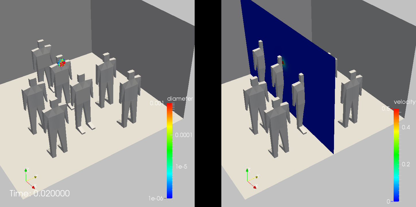
Figure 5. TSA Queue: Particle Distribution at $t=0.02~{}sec$

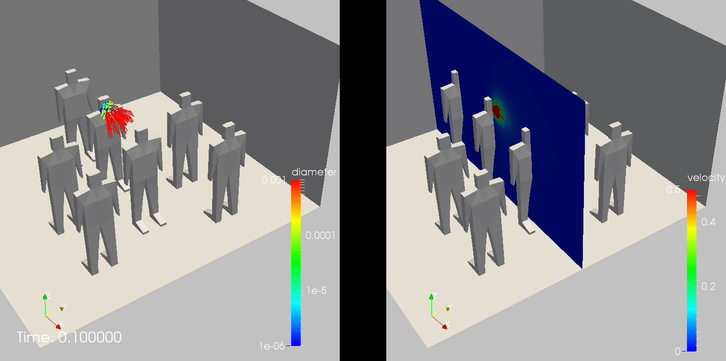
Figure 6. TSA Queue: Particle Distribution at $t=0.10~{}sec$

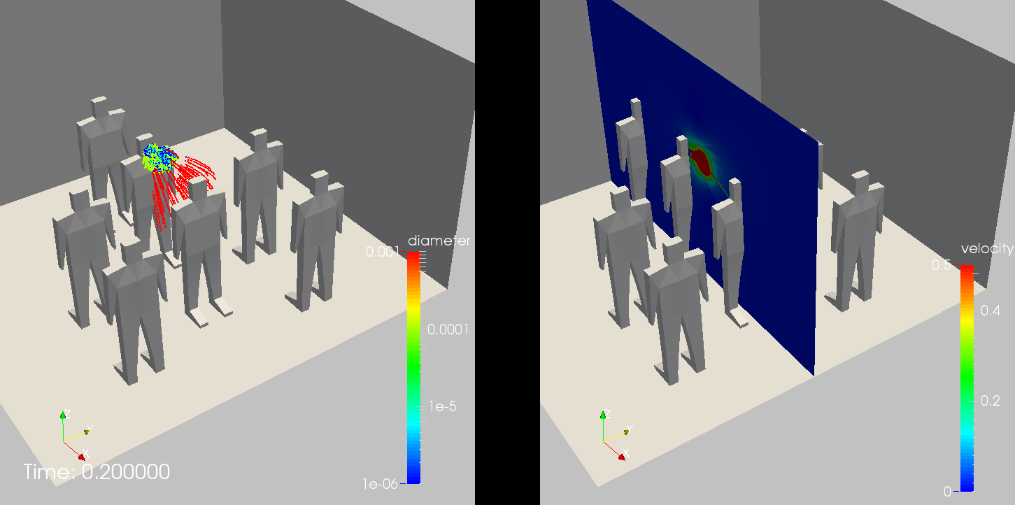
Figure 7. TSA Queue: Particle Distribution at $t=0.20~{}sec$

Figure 8. TSA Queue: Particle Distribution at $t=0.40~{}sec$

Figure 9. TSA Queue: Particle Distribution at $t=0.80~{}sec$

Figure 10. TSA Queue: Particle Distribution at $t=1.60~{}sec$

6.2. Sneezing in a Generic Hospital Room

This case considers a typical hospital room. Of interest here was the dispersion of particles in the first minute after coughing, in particular the reach into neighbouring halls and the amount of ‘negative pressure’ needed to keep all contaminants in the room. Figure 11 shows the arrangement of the room, with patient and caregiver clearly visible. This particular mesh had 2.25Mels. The distribution of particles over time can be discerned from Figures 12-22. As before, one can see that the large (red) particles follow a ballistic path. This ‘ballistic phase’ ends at about $t=1~{}sec$. The (green) particles of size $d=0.1~{}mm$ are quickly stopped by the air, and then sink slowly towards the patient. The even smaller (cyan, blue) particles rise with the cloud of warmer air exhaled by the sneezing individual, and disperse much further at later times, covering almost the entire room. The velocity distribution in the room may be inferred from Figure 23.

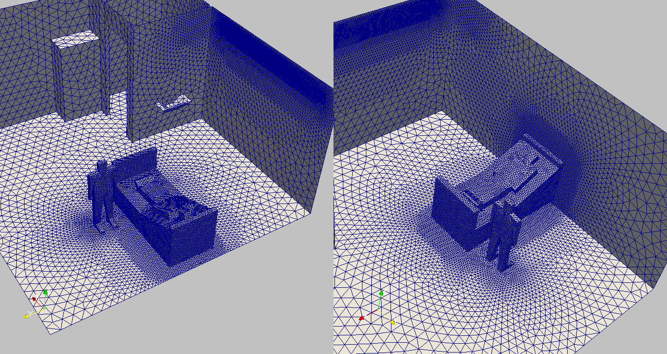
Figure 11. Hospital Room: Surface Mesh

Figure 12. Hospital Room: Particle Distribution at t=0.0 sec

Figure 13. Hospital Room: Particle Distribution at t=0.2 sec

Figure 14. Hospital Room: Particle Distribution at t=0.4 sec

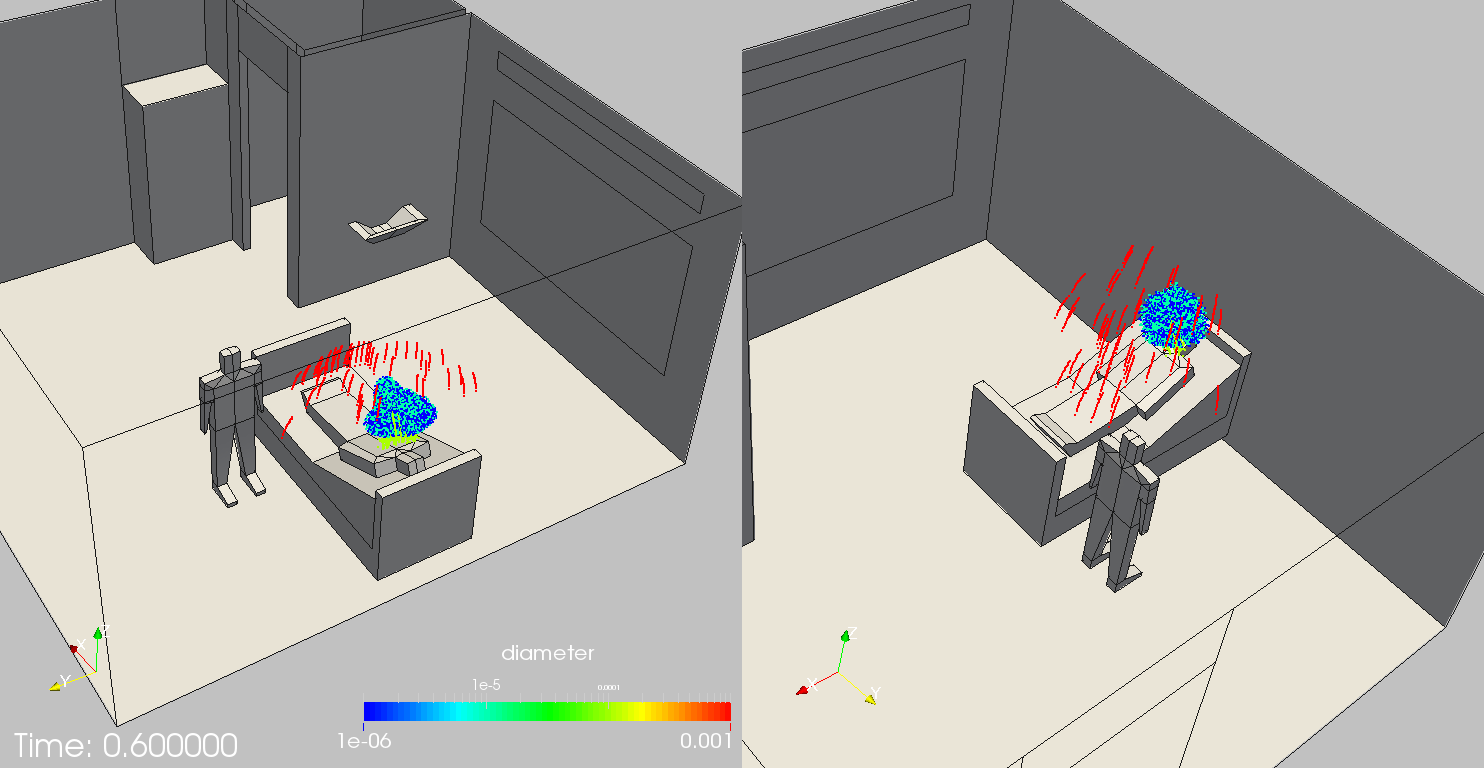
Figure 15. Hospital Room: Particle Distribution at t=0.6 sec

Figure 16. Hospital Room: Particle Distribution at t=1.0 sec

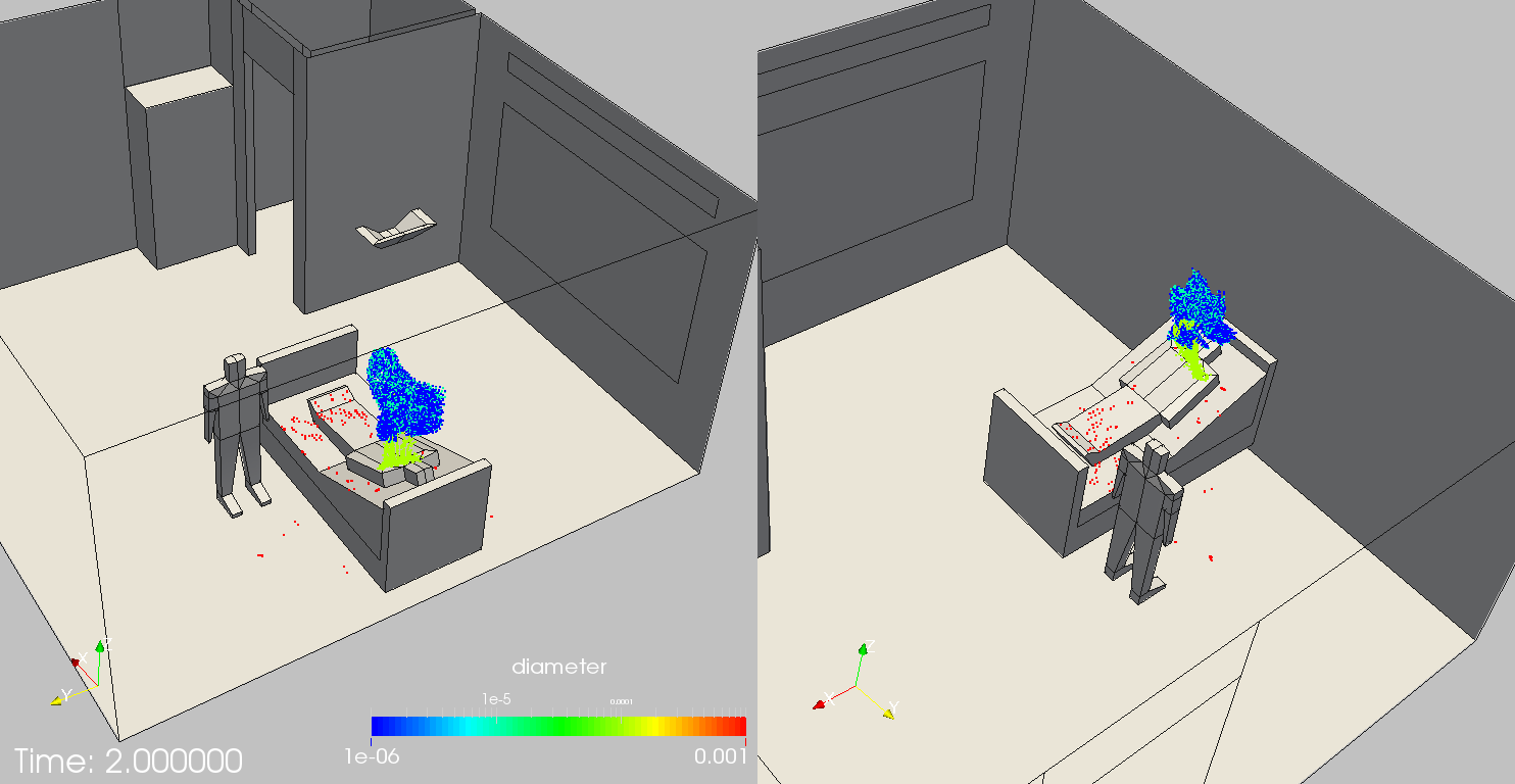
Figure 17. Hospital Room: Particle Distribution at t=2.0 sec

Figure 18. Hospital Room: Particle Distribution at t=4.0 sec

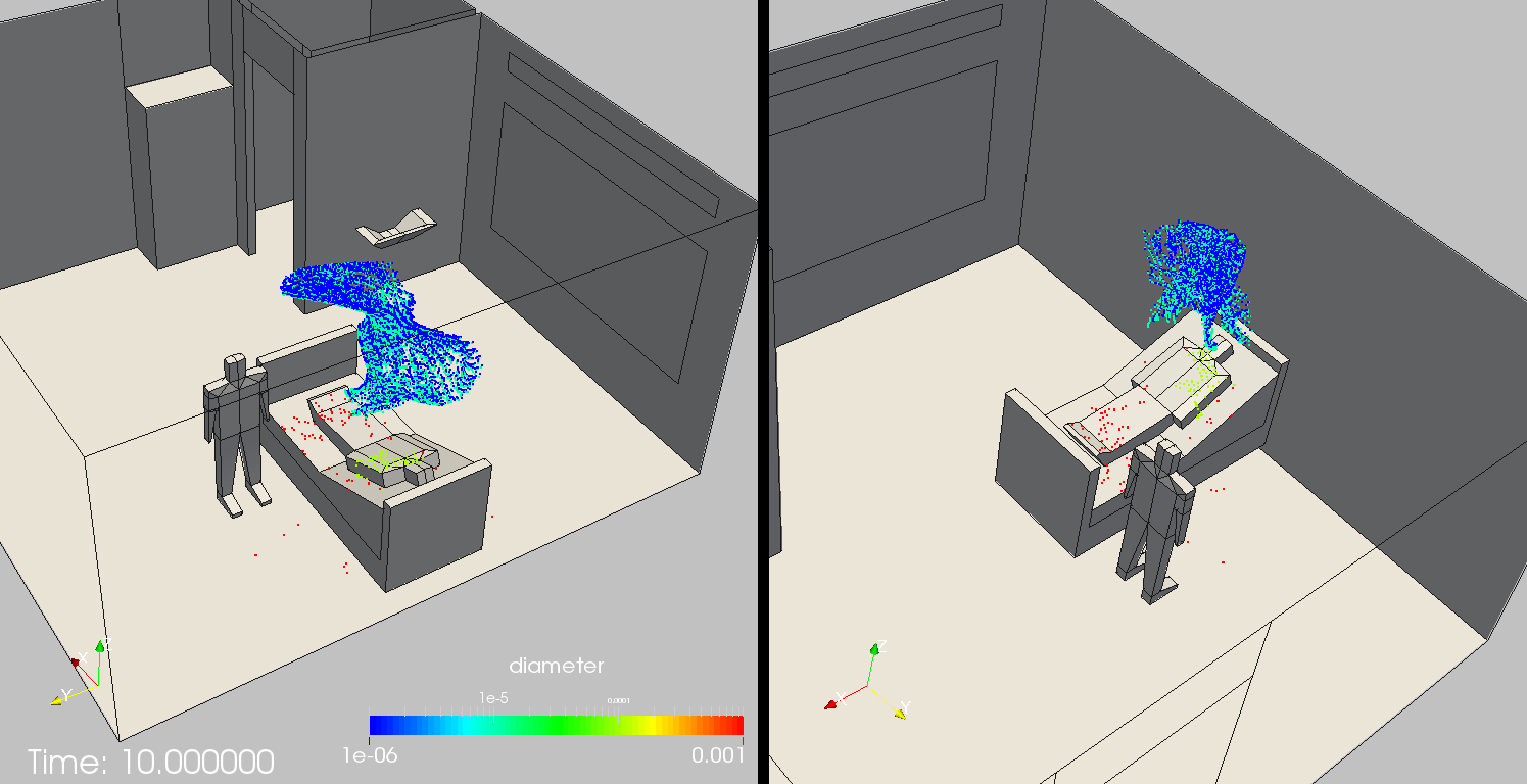
Figure 19. Hospital Room: Particle Distribution at t=10.0 sec

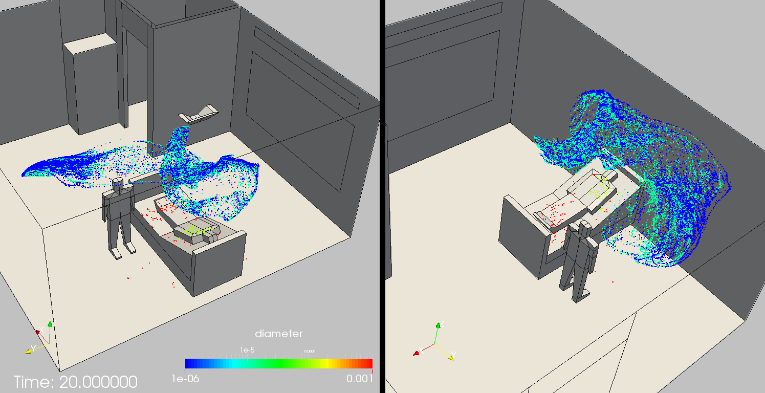
Figure 20. Hospital Room: Particle Distribution at t=20.0 sec

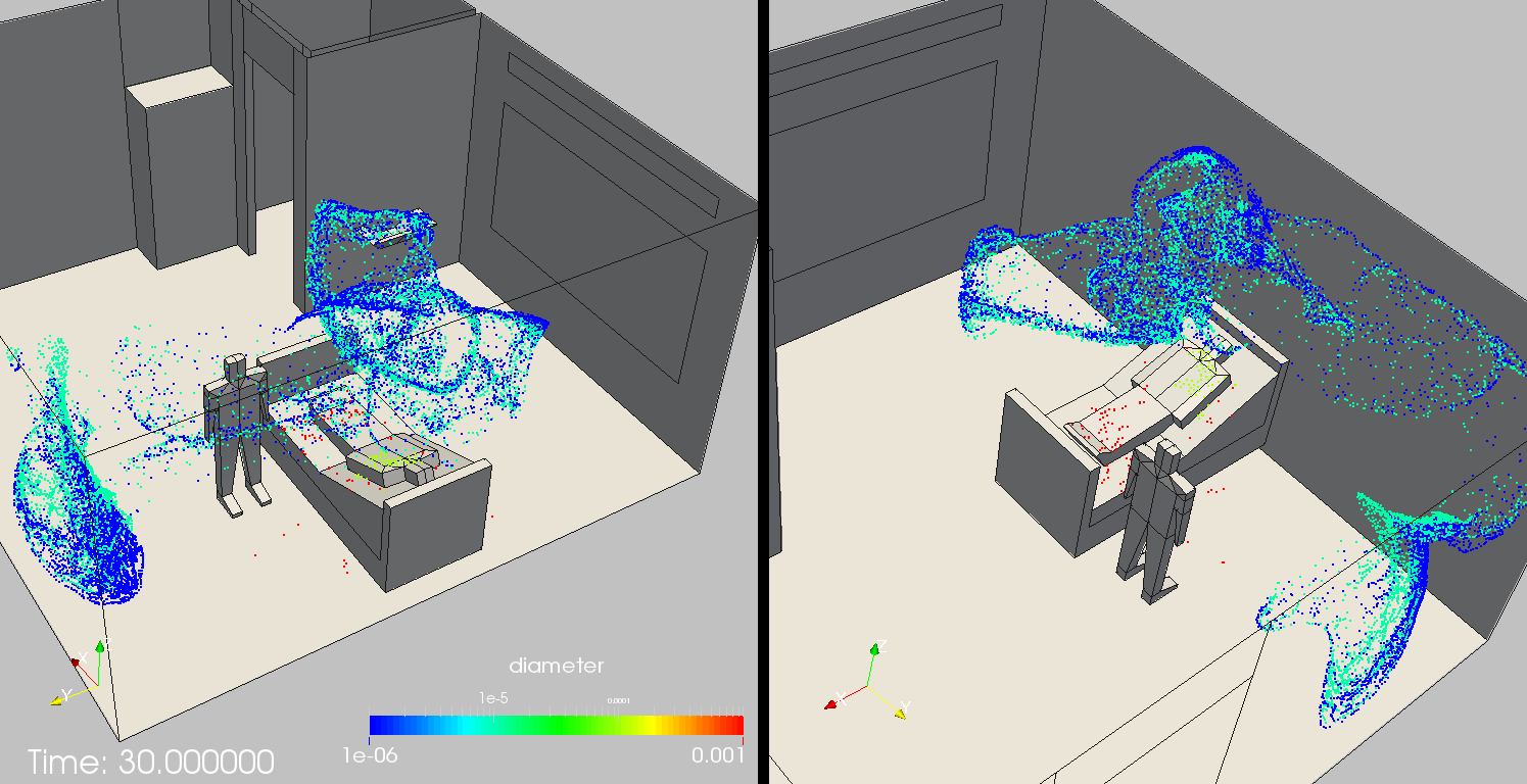
Figure 21. Hospital Room: Particle Distribution at t=30.0 sec

Figure 22. Hospital Room: Particle Distribution at t=50.0 sec

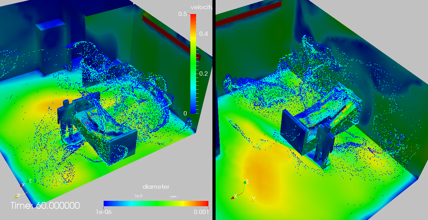
Figure 23. Hospital Room: Surface Velocities at t=60.0 sec

7. Reopening After the Crisis

A lingering question facing all levels of society is how and when to reopen facilities where people congregate in close proximity. One key technology that would allow opening is testing and sensing. We consider sensing in the sequel. Several vendors have announced measuring devices for Covid-19 in the next half year. Given that these sensors are expensive, and that a hospital or university many need hundreds of these, the question becomes how best to deploy them. In other words: given an arbitrary number of contamination or infection scenarios, which is the minimum number of sensors needed to detect them, and where should they be placed ? A partial answer to this non-trivial question was given in [67, 110]. If we assume a given number of sensors, every contaminant/infection scenario (location and amount of release, flow conditions, etc.) will lead to a sensor input. The data recorded from all the possible release scenarios at all possible sensor locations allows the identification of the best or optimal sensor locations. Clearly, if only one sensor is to be placed, it should be at the location that recorded the highest number of releases. This argument can be used recursively by removing from further consideration all releases already recorded by sensors previously placed. The procedure is repeated recursively until no undetected release cases are left, or the available sensors have been exhausted.
See [21, 45] for an in-depth analysis of robust sensor placement under uncertainty.

7.1. Hospital Room

This case considers the same hospital room as shown before. The boundary conditions determining the flow are assumed as steady, with air entering the room through vents 1-3 and exiting the room through the bathroom exhaust or the door. Figures 24-26 show the outlay of the room, average velocities and the ‘age of air’ after 5 minutes. Note the high values for the age of air in the corners and the back of the room. This particular mesh had 2.2Mels. Four contaminant release scenarios were considered: cases 1-3 assumed contaminant coming in through each of the vents (separately) during the first minute, while case 4 assumed virus production from the patient for a period of 10 seconds. The case was run for 5 minutes of real time, and the contaminant concentration was measured on all walls/ceilings. The maximum concentrations measured have been summarized in Figure 27. Note the different areas covered depending on the release scenario. It was assumed that sensors should only be allowed above a certain height, and should be located on a wall or the ceiling. Table 4 summarizes the points that measured data above a set threshold. As one can see, none of the possible sensor locations is able to measure/detect all 4 cases, and many possible sensor locations do not detect even a single case. There are many possible pairs of sensors that can detect all 4 cases. The pair selected is the one that achieves the highest relative measurement values, and is shown in Figure 28. Note that this makes good sense: one sensor close the HVAC exits, and one close to the patient.

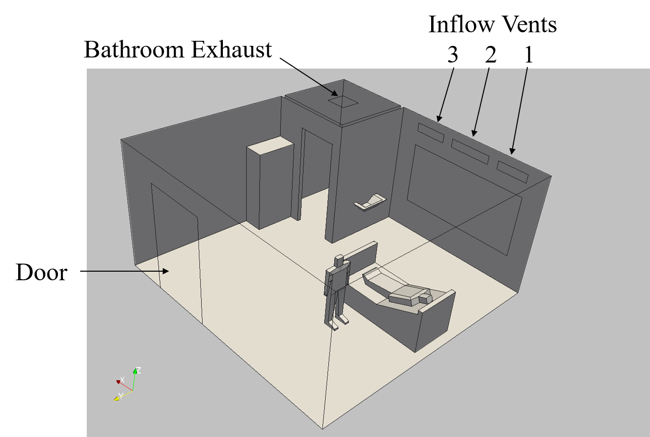
Figure 24. Hospital Room: Outlay of Room and Boundary Conditions

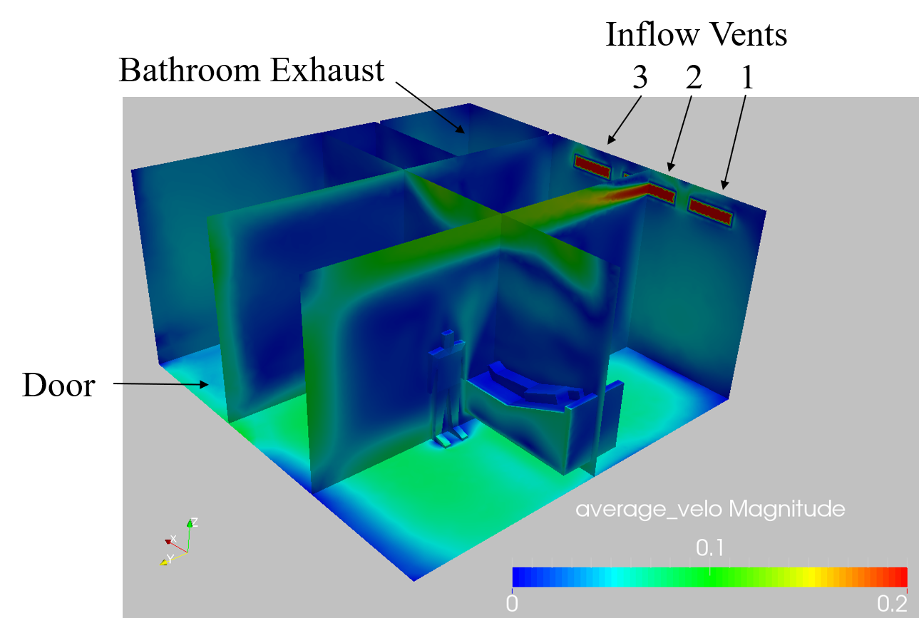
Figure 25. Hospital Room: Average Velocities (5 mins)

Figure 26. Hospital Room: Age of Air (5 mins)

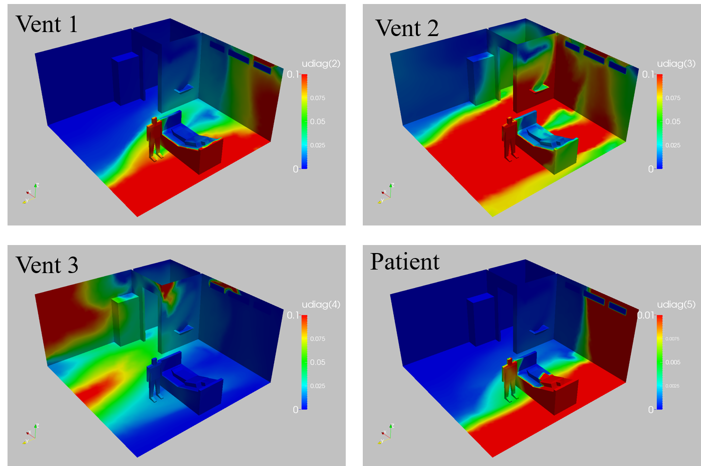
Figure 27. Hospital Room: Maximum Contaminant Concentration Over 5 Minutes

Table 4. Data Measurement Summary

Cases Measured	Number
0	4308
1	3377
2	1010
3	0
4	0

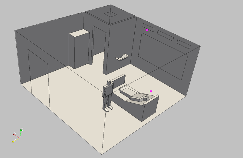
Figure 28. Hospital Room: Optimal Sensor Locations

8. Conclusions and Outlook

The present paper has summarized some of the mechanical characteristics of virus contaminants and the transmission via droplets and aerosols. The ordinary and partial differential equations describing the physics of these processes with high fidelity were given, as well as appropriate numerical schemes to solve them. Several examples taken from recent evaluations of the built environment were given, as well as the optimal placement of sensors.

Current efforts are directed at increasing the realism of the physical processes modeled (e.g. by adding the effect of moving pedestrians [79]), streamlining the simulation toolbox and workflow, and fielding these tools so that the post-pandemic opening can occur as smoothly as possible.

References

- [1] S. Appanaboyina, F. Mut, R. Löhner, C. M. Putman and J. R. Cebral - Computational Fluid Dynamics of Stented Intracranial Aneurysms Using Adaptive Embedded Unstructured Grids; Int. J. Num. Meth. Fluids 57, 5, 475-493 (2008).
- [2] S. Asadi, A.S. Wexler, C.D. Cappa, S. Barreda, N.M. Bouvier and W. Ristenpart - Aerosol Emission and Superemission During Human Speech Increase with Voice Loudness; Nature Scientific Reports 9, (1):2348 (2019). www.nature.com/scientificreports/ https://doi.org/10.1038/s41598-019-38808-z
- [3] S. Asadi, A.S. Wexler, C.D. Cappa, S. Barreda, N.M. Bouvier and W. Ristenpart - Effect of Voicing and Articulation Manner on Aerosol Particle Emission During Human Speech PLoS ONE 15(1):e0227699 (2020). https://doi.org/10.1371/journal.pone.0227699
- [4] S. Asadi, N.M. Bouvier, A.S. Wexler and W. Ristenpart - The Coronavirus Pandemic and Aerosols: Does COVID-19 Transmit via Expiratory Particles ? Aerosol Science and Technology (2020). https://doi.org/10.1080/02786826.2020.1749229
- [5] R. Aubry, F. Mut, R. Löhner and J. R. Cebral - Deflated Preconditioned Conjugate Gradient Solvers for the Pressure-Poisson Equation; J. Comp. Phys. 227, 24, 10196-10208 (2008).
- [6] J.D. Baum and R. Löhner - Numerical Simulation of Shock Interaction with a Modern Main Battlefield Tank; AIAA-91-1666 (1991).
- [7] J.D. Baum and R. Löhner - Numerical Simulation of Pilot/Seat Ejection from an F-16; AIAA-93-0783 (1993).
- [8] J.D. Baum. H. Luo and R. Löhner - Numerical Simulation of a Blast Inside a Boeing 747; AIAA-93-3091 (1993).
- [9] J.D. Baum, H. Luo and R. Löhner - Numerical Simulation of a Blast Withing a Multi-Room Shelter; pp. 451-463 in Proc. MABS-13 Conf. The Hague, Netherlands, September (1993).
- [10] J.D. Baum, H. Luo and R. Löhner - A New ALE Adaptive Unstructured Methodology for the Simulation of Moving Bodies; AIAA-94-0414 (1994).
- [11] J.D. Baum, H. Luo and R. Löhner - Numerical Simulation of Blast in the World Trade Center; AIAA-95-0085 (1995).
- [12] J.D. Baum, H. Luo and R. Löhner - Validation of a New ALE, Adaptive Unstructured Moving Body Methodology for Multi-Store Ejection Simulations; AIAA-95-1792 (1995).
- [13] J.D. Baum, H. Luo, R. Löhner, C. Yang, D. Pelessone and C. Charman - Coupled Fluid/Structure Modeling of Shock Interaction with a Truck; AIAA-96-0795 (1996).
- [14] J.D. Baum, H. Luo, R. Löhner, E. Goldberg and A. Feldhun - Application of Unstructured Adaptive Moving Body Methodology to the Simulation of Fuel Tank Separation from an F-16 c/d Fighter; AIAA-97-0166 (1997).
- [15] J.D. Baum, R. Löhner, T.J. Marquette and H. Luo - Numerical Simulation of Aircraft Canopy Trajectory; AIAA-97-1885 (1997).
- [16] J.D. Baum, H. Luo, E. Mestreau, R. Löhner, D. Pelessone and C. Charman - Coupled CFD/CSD Methodology for Modeling Weapon Detonation and Fragmentation; AIAA-99-0794 (1999).
- [17] J.D. Baum, E. Mestreau, H. Luo, R. Löhner, D. Pelessone, M.E. Giltrud and J.K. Gran - Modeling of Near-Field Blast Wave Evolution; AIAA-06-0191 (2006).
- [18] K. Balakrishnan and S. Menon - On the Role of Ambient Reactive Particles in the Mixing and Afterburn Behind Explosive Blast Waves; Combust. Sci. and Tech. 182, 186–214 (2010).
- [19] K. Benkiewicz and K. Hayashi - Two-Dimensional Numerical Simulations of Multi-Headed Detonations in Oxygen-Aluminum Mixtures Using an Adaptive Mesh Refinement; Shock Waves , 12, 5, 385-402 (2003).
- [20] J.P. Boris, F.F. Grinstein, E.S. Oran, and R.J. Kolbe - New Insights Into Large Eddy Simulation; Fluid Dynamics Research 10, 199-228 (1992).
- [21] J.A. Burns and C.N. Rautenberg - The Infinite-Dimensional Optimal Filtering Problem with Mobile and Stationary Sensor Networks; Numerical Functional Analysis and Optimization 36, 2, 181-224 (2015). https://doi.org/10.1080/01630563.2014.970647
- [22] F. Camelli and R. Löhner - Assessing Maximum Possible Damage for Contaminant Release Events; Engineering Computations 21, 7, 748-760 (2004).
- [23] F. Camelli, R. Löhner, W.C. Sandberg and R. Ramamurti - VLES Study of Ship Stack Gas Dynamics; AIAA-04-0072 (2004).
- [24] F. Camelli and R. Löhner - VLES Study of Flow and Dispersion Patterns in Heterogeneous Urban Areas; AIAA-06-1419 (2006).
- [25] F. Camelli, J. Lien, D. Dayong, D. W. Wong, M. Rice, R. Löhner and C. Yang - Generating Seamless Surfaces for Transport and Dispersion Modeling in GIS; submitted to GeoInformatica 16, 2, 207-327 (2012).
- [26] J.R. Cebral and R. Löhner - From Medical Images to Anatomically Accurate Finite Element Grids; Int. J. Num. Meth. Eng. 51, 985-1008 (2001).
- [27] J.R. Cebral and R. Löhner - Efficient Simulation of Blood Flow Past Complex Endovascular Devices Using an Adaptive Embedding Technique; IEEE Transactions on Medical Imaging 24, 4, 468-476 (2005).
- [28] C. Chao, M.P. Wan, L. Morawska, G. Johnson, R. Graham, Z. Ristovski M. Hargreaves, K. Mengersen, L. Kerrie C. Steve, Y. Li, X. Xie and S. Katoshevski - Characterization of Expiration Air Jets and Droplet Size Distributions Immediately at the Mouth Opening; J. of Aerosol Science 40, 2, 122-133 (2009).
- [29] R. Clift, J.R. Grace and M.E. Weber - Bubbles, Drops and Particles; Academic Press, New York (1978).
- [30] A. Corrigan, F. Camelli and R. Löhner - Porting Of An Edge-Based CFD Solver to GPUs; AIAA-10-0523 (2010).
- [31] A. Corrigan, F. Camelli, R. Löhner and F. Mut - Porting of FEFLO to GPUs; Proc. ECCOMAS CFD 2010 Conf. Lisbon, Portugal, June 14-17 (2010).
- [32] A. Corrigan, F.F. Camelli, R. Löhner and J. Wallin - Running Unstructured Grid Based CFD Solvers on Modern Graphics Hardware; Int. J. Num. Meth. Fluids 66, 221-229 (2011).
- [33] A. Corrigan and R. Löhner - Porting of FEFLO to Multi-GPU Clusters; AIAA-11-0948 (2011).
- [34] N.G. Deen, M. v.Sint Annaland and J.A.M. Kuipers - Direct Numerical Simulation of Particle Mixing in Dispersed Gas-Liquid-Solid Flows Using a Combined Volume of Fluid and Discrete Particle Approach; Proc. Fifth Int. Conf. on CFD in the Process Industries, CSIRO, Melbourne, Australia, 13-15 December (2006).
- [35] L. Dietz, P.F. Horve, D.A. Coil, M. Fretz, J.A. Eisen and L. van den Wymelenberg - 2019 Novel Coronavirus (COVID-19) Pandemic: Built Environment Considerations to Reduce Transmission; mSystems 5:e00245-20 (2020). doi:10.1128/mSystems.00245-20.
- [36] P. Fabian, J.J. McDevitt, W.H. Dehaan, R.O.P. Fung, B.J. Cowling, K.H. Chan, et al. - Influenza Virus in Human Exhaled Breath: An Observational Study; PLoS ONE 3:e2691 (2008).
- [37] D.R. Franz, P.B. Jahrling, A.M. Friedlander, et al. - Clinical Recognition and Management of Patients Exposed to Biological Warfare Agents; JAMA 278:399e411 (1997).
- [38] C. Fureby and F. Grinstein - Monotonically Integrated Large Eddy Simulation of Free Shear Flows; AIAA J. 37, 5, 544-556 (1999).
- [39] F.F. Grinstein and C. Fureby - Recent Progress on MILES for High-Reynolds-Number Flows; J. Fluids Engineering 124, 848-861 (2002).
- [40] J.K. Gupta, C-H. Lin and Q. Chen - Flow Dynamics and Characterization of a Cough; Indoor Air 19, 517–525 (2009).
- [41] J.K. Gupta, C-H. Lin and Q. Chen - Characterizing Exhaled Airflow from Breathing and Talking; Indoor Air 20, 31-39 (2010).
- [42] J.K. Gupta, C-H. Lin and Q. Chen - Inhalation of Expiratory Droplets in Aircraft Cabins; Indoor Air 21, 341-350 (2011). doi:10.1111/j.1600-0668.2011.00709.x
- [43] J.K. Gupta, C-H. Lin and Q. Chen - Transport of Expiratory Droplets in an Aircraft Cabin; Indoor Air 21, 3-11 (2011).
- [44] S.K. Halloran, A.S. Wexler and W.D. Ristenpart - A Comprehensive Breath Plume Model for Disease Transmission via Expiratory Aerosols; PLoS ONE 7(5):e37088 (2012). https://doi.org/10.1371/journal.pone.0037088
- [45] M. Hintermüller, C.N. Rautenberg, M. Mohammadi and M. Kanitsar - Optimal Sensor Placement: A Robust Approach; SIAM J. Control Optim. 55(6), 3609-3639 (2017). https://doi.org/10.1137/16M1088867
- [46] J. Hoberock and N. Bell - Thrust: Parallel Template Library, Version 1.3 (2010).
- [47] S.R. Idelsohn, N. Nigro, A. Larreteguy, J.M. Gimenez and P. Ryshakov - A Pseudo-DNS Method for the Simulation of Incompressible Fluid Flows with Instabilities at Different Scales; Int. J. Comp. Particle Mechanics (2019). https://doi.org/10.1007/s40571-019-00264-x
- [48] M. Ip, J.W. Tang, D.S.C. Hui, A.L.N. Wong, M.T.V. Chan, G.M. Joynt, A.T.P. So, S.D. Hall, P.K.S. Chan and J.J.Y. Sung - Airflow and Droplet Spreading Around Oxygen Masks: A Simulation Model for Infection Control Research; AJIC 35, 10, 684-689 (2007).
- [49] A. Jameson, W. Schmidt and E. Turkel - Numerical Solution of the Euler Equations by Finite Volume Methods using Runge-Kutta Time-Stepping Schemes; AIAA-81-1259 (1981).
- [50] G.R. Johnson, L. Morawska, Z.D. Ristovski, M. Hargreaves, K. Mengersen, C.Y.H. Chao, M.P. Wan, Y. Li , X. Xie, D. Katoshevski, S. Corbette - Modality of Human Expired Aerosol Size Distributions J. of Aerosol Science 42, 839-851 (2011).
- [51] G. Kampf, D. Todt, S. Pfaender, E. Steinmann - Persistence of Coronaviruses on Inanimate Surfaces and Their Inactivation With Biocidal Agents; J. of Hospital Infection 104, 3, 246-251, March 01 (2020). https://doi.org/10.1016/j.jhin.2020.01.022
- [52] C.K. Kim, J.G. Moon, J.S. Hwang, M.C. Lai and K.S. Im - Afterburning of TNT Explosive Products in Air With Aluminum Particles; AIAA-2008-1029 (2008).
- [53] Y.-I. Kim et al. - Infection and Rapid Transmission of SARS-CoV-2 in Ferrets; Cell Host and Microbe 27, 1-6 (2020). https://doi.org/10.1016/j.chom.2020.03.023
- [54] Y. Li et al. - Role of Ventilation in Airborne Transmission of Infactious Agents in the Built Environment - A Multidisciplinary Systematic Review; Indoor Air 17, 2-18 (2007).
- [55] W.G. Lindsley, F.M. Blachere, R.E. Thewlis, A. Vishnu, K.A. Davis, G. Cao, et al. - Measurements of Airborne Influenza Virus in Aerosol Particles from Human Coughs; PLoS ONE 5:e15100 (2010).
- [56] W.G. Lindsley, T.A. Pearce, J.B. Hudnall, K.A. Davis, S.M. Davis, M.A. Fisher, et al. - Quantity and Size Distribution of Cough-Generated Aerosol Particles Produced by Influenza Patients During and After Illness; J. Occup. Environ. Hyg. 9, 443-9. (2012).
- [57] J. Liu, K. Kailasanath, R. Ramamurti, D. Munday, E. Gutmark and R. Löhner - Large-Eddy Simulations of a Supersonic Jet and Its Near-Field Acoustic Properties; AIAA J. 47, 8, 1849-1864 (2009).
- [58] R. Löhner, K. Morgan, J. Peraire and M. Vahdati - Finite Element Flux-Corrected Transport (FEM-FCT) for the Euler and Navier-Stokes Equations; Int. J. Num. Meth. Fluids 7, 1093-1109 (1987).
- [59] R. Löhner and J. Ambrosiano - A Vectorized Particle Tracer for Unstructured Grids; J. Comp. Phys. 91, 1, 22-31 (1990).
- [60] R. Löhner and R. Ramamurti - A Load Balancing Algorithm for Unstructured Grids; Comp. Fluid Dyn. 5, 39-58 (1995).
- [61] R. Löhner - Renumbering Strategies for Unstructured-Grid Solvers Operating on Shared-Memory, Cache-Based Parallel Machines; Comp. Meth. Appl. Mech. Eng. 163, 95-109 (1998).
- [62] R. Löhner, C. Yang and E. Oñate - Viscous Free Surface Hydrodynamics Using Unstructured Grids; Proc. 22nd Symp. Naval Hydrodynamics, Washington, D.C., August (1998).
- [63] R. Löhner, Chi Yang, J. Cebral, O. Soto, F. Camelli, J.D. Baum, H. Luo, E. Mestreau, D. Sharov, R. Ramamurti, W. Sandberg and Ch. Oh - Advances in FEFLO; AIAA-01-0592 (2001).
- [64] R. Löhner and M. Galle - Minimization of Indirect Addressing for Edge-Based Field Solvers; Comm. Num. Meth. Eng. 18, 335-343 (2002).
- [65] R. Löhner - Multistage Explicit Advective Prediction for Projection-Type Incompressible Flow Solvers; J. Comp. Phys. 195, 143-152 (2004).
- [66] R. Löhner, J.D. Baum and D. Rice - Comparison of Coarse and Fine Mesh 3-D Euler Predictions for Blast Loads on Generic Building Configurations; Proc. MABS-18 Conf., Bad Reichenhall, Germany, September (2004).
- [67] R. Löhner and F. Camelli - Optimal Placement of Sensors for Contaminant Detection Based on Detailed 3-D CFD Simulations; Engineering Computations 22, 3, 260-273 (2005).
- [68] R. Löhner, Chi Yang, J.R. Cebral, F. Camelli, O. Soto and J. Waltz - Improving the Speed and Accuracy of Projection-Type Incompressible Flow Solvers; Comp. Meth. Appl. Mech. Eng. 195, 23-24, 3087-3109 (2006).
- [69] R. Löhner, Chi Yang and E. Oñate - On the Simulation of Flows with Violent Free Surface Motion; Comp. Meth. Appl. Mech. Eng. 195, 5597-5620 (2006).
- [70] R. Löhner, Chi Yang and E. Oñate - Simulation of Flows With Violent Free Surface Motion and Moving Objects Using Unstructured Grids; Int. J. Num. Meth. Fluids 53, 1315-1338 (2007).
- [71] R. Löhner - Applied CFD Techniques, Second Edition; J. Wiley & Sons (2008).
- [72] R. Löhner, H. Luo, J.D. Baum and D. Rice - Improvements in Speed for Explicit, Transient Compressible Flow Solvers; Int. J. Num. Meth. Fluids 56, 12, 2229-2244 (2008).
- [73] R. Löhner, J.R. Cebral, F.F. Camelli, S. Appanaboyina, J.D. Baum, E.L. Mestreau and O. Soto - Adaptive Embedded and Immersed Unstructured Grid Techniques; Comp. Meth. Appl. Mech. Eng. 197, 2173-2197 (2008).
- [74] R. Löhner, F. Mut and F.F. Camelli - Timings OF FEFLO on the SGI-ICE Machines; AIAA-11-1064 (2011).
- [75] R. Löhner and A. Corrigan - Semi-Automatic Porting if a General Fortran CFD Code to GPUs: The Difficult Modules; AIAA-11-3219 (2011).
- [76] R. Löhner, F. Mut, J.R. Cebral, R. Aubry and G. Houzeaux; Deflated Preconditioned Conjugate Gradient Solvers for the Pressure-Poisson Equation: Extensions and Improvements; Int. J. Num. Meth. Eng. 87, 1-5, 2-14 (2011).
- [77] R. Löhner - F2GPU - A General Fortran to GPU Translator; Proc. NVIDIA GTC Conf. , San Jose, CA, May (2012).
- [78] R. Löhner, F. Camelli, J.D. Baum, F. Togashi and O. Soto - On Mesh-Particle Techniques; Comp. Part. Mech. 1, 199-209 (2014).
- [79] R. Löhner and F. Camelli - Tightly Coupled Computational Fluid and Crowd Dynamics; pp. 505-509 in Proc. Pedestrian and Evacuation Dynamics 2016 (PED 2016), (W. Song, J. Ma and L. Fu eds.), University of Science and Technology Press, Hefei, China, Oct 17-21 (2016).
- [80] R.G. Loudon and R.M. Roberts - Droplet Expulsion from the Respiratory Tract; Am. Rev. Respir. Dis. 95, 3, 435–442 (1967).
- [81] H. Luo, J.D. Baum and R. Löhner - Edge-Based Finite Element Scheme for the Euler Equations; AIAA J. 32, 6, 1183-1190 (1994).
- [82] H. Luo, J.D. Baum, R. Löhner and J. Cabello - Implicit Finite Element Schemes and Boundary Conditions for Compressible Flows on Unstructured Grids; AIAA-94-0816 (1994).
- [83] H. Luo, J.D. Baum and R. Löhner - An Accurate, Fast, Matrix-Free Implicit Method for Computing Unsteady Flows on Unstructured Grids; AIAA-99-0937 (1999).
- [84] H. Luo, D. Sharov, J.D. Baum and R. Löhner - A Class of Matrix-free Implicit Methods for Compressible Flows on Unstructured Grids; First International Conference on Computational Fluid Dynamics, Kyoto, Japan, July 10-14 (2000).
- [85] H. Luo, J.D. Baum and R. Löhner - A Fast, Matrix-Free Implicit Method for Computing Low Mach Number Flows on Unstructured Grids; Int. J. CFD 14, 133-157 (2001).
- [86] D. Merrill and A. Grimshaw - Revisiting Sorting for GPGPU Stream Architectures; UVA CS Rep. CS2010-03, Charlottesville, VA (2010).
- [87] D.K. Milton, M.P. Fabian, B.J. Cowling, M.L. Grantham, J.J. McDevitt - Influenza Virus Aerosols in Human Exhaled Breath: Particle Size, Culturability, and Effect of Surgical Masks; PLoS Pathog. 9:e1003205 (2013).
- [88] NVIDIA Corporation. NVIDIA CUDA 3.2 Programming Guide (2010).
- [89] J. Peraire, M. Vahdati, K. Morgan and O.C. Zienkiewicz - Adaptive Remeshing for Compressible Flow Computations; J. Comp. Phys. 72, 449-466 (1987).
- [90] P. Peterson - F2PY: Tool for Connecting Fortran and Python Programs; Int. J. Computational Science and Engineering 4, 296-305 (2009).
- [91] R. Ramamurti and R. Löhner - Simulation of Flow Past Complex Geometries Using a Parallel Implicit Incompressible Flow Solver; pp. 1049,1050 in Proc. 11th AIAA CFD Conf. , Orlando, FL, July (1993).
- [92] R. Ramamurti and R. Löhner - A Parallel Implicit Incompressible Flow Solver Using Unstructured Meshes; Computers and Fluids 5, 119-132 (1996).
- [93] R. Ramamurti, W.C. Sandberg and R. Löhner - Computation of Unsteady Flow Past Deforming Geometries; Int. J. Comp. Fluid Dyn. , 83-99 (1999).
- [94] D.L. Rice, J.D. Baum, F. Togashi, R. Löhner and A. Amini - First-Principles Blast Diffraction Simulations on a Notebook: Accuracy, Resolution and Turn-Around Issues; Proc. MABS-20 Conf., Oslo, Norway, September (2008).
- [95] H. Schlichting - Boundary Layer Theory; McGraw-Hill (1979).
- [96] D. Sharov, H. Luo, J.D. Baum and R. Löhner - Implementation of Untructured Grid GMRES+LU-SGS Method on Shared-Memory, Cache-Based Parallel Computers; AIAA-00-0927 (2000).
- [97] A. Stück, F. Camelli and R. Löhner - Adjoint-Based Design of Shock Mitigation Devices; Int. J. Num. Meth. Fluids 64, 443-472 (2010).
- [98] J.W. Tang, Y. Li, I. Eames, P.K.S. Chan and G.L. Ridgway Factors Involved in the Aerosol Transmission of Infection and Control of Ventilation in Healthcare Premises; J. of Hospital Infection 64, 100-114 (2006).
- [99] J.W. Tang, C.J. Noakes, P.V. Nielsen, I. Eames, A. Nicolle, Y. Li and G.S. Settles - Observing and Quantifying Airflows in the Infection Control of Aerosol- and Airborne-Transmitted Diseases: An Overview of Approaches; J. of Hospital Infection 77 213-222 (2011).
- [100] J.W. Tang, A.D. Nicolle, J. Pantelic, G.C. Koh, L. Wang, M. Amin, C.A. Klettner, D.K.W. Cheong, C. Sekhar and K.W. Tham - Airflow Dynamics of Coughing in Healthy Human Volunteers by Shadowgraph Imaging: An Aid to Aerosol Infection Control; PLoS ONE 7, 4: e34818 (2012). doi:10.1371/journal.pone.0034818
- [101] J.W. Tang, A.D. Nicolle, C.A. Klettner, J. Pantelic, L. Wang, A. Bin Suhaimi, A.Y.L. Tan, G.W.X. Ong, R. Su, C. Sekhar, D.K.W. Cheong and K.W. Tham - Airflow Dynamics of Human Jets: Sneezing and Breathing - Potential Sources of Infectious Aerosols; PLoS ONE 8, 4: e59970 (2013). doi:10.1371/journal.pone.0059970
- [102] P.F.M. Teunis, N. Brienen, M.E.E. Kretzschmar - High Infectivity and Pathogenicity of Influenza A Virus Via Aerosol and Droplet Transmission; Epidemics 2, 215–222 (2010).
- [103] R. Tilch, A. Tabbal, M. Zhu, F. Decker and R. Löhner - Combination of Body-Fitted and Embedded Grids for External Vehicle Aerodynamics; Engineering Computations 25, 1, 28-41 (2008).
- [104] K. K.-W. To et al. - Temporal Profiles of Viral Load in Posterior Oropharyngeal Saliva Samples and Serum Antibody Responses During Infection by SARS-CoV-2: An Observational Cohort Study; Lancet Infect. Dis. (online) (2020). https://doi.org/10.1016/S1473-3099(20)30196-1
- [105] F. Togashi, J.D. Baum, E. Mestreau, R. Löhner, and D. Sunshine; Numerical Modeling of Long-Duration Blast Wave Evolution in Confined Facilities; AIAA-09-1531 (2009).
- [106] N. van Doremalen, T. Bushmaker, D.H. Morris, M.G. Holbrook, A. Gamble, B.N. Williamson, A. Tamin, J.L. Harcourt, N.J. Thornburg, S.I. Gerber, J.O. Lloyd-Smith, E. de Wit, V.J. Munster - Aerosol and Surface Stability of SARS-CoV-2 as Compared with SARS-CoV-1; The New England Journal of Medicine 382, 16, April 16 (2020). DOI: 10.1056/NEJMc2004973
- [107] A.W. Vreman, B.J. Geurts, N.G. Deen and J.A.M. Kuipers - Large-Eddy Simulation of a Particle Laden Turbulent Channel Flow; Proc. Direct and Large-Eddy Simulation V, ERCOFTAC Series Volume 9, pp 271-278 (2004).
- [108] J. Wei, Y. Li - Airborne Spread of Infectious Agents in the Indoor Environment; American J. of Infection Control 44, S102-S108 (2016). http://dx.doi.org/10.1016/j.ajic.2016.06.003
- [109] X. Xie, Y. Li, A.T.Y. Chwang, P.L. Ho, W.H. Seto - How Far Droplets Can Move in Indoor Environments - Revisiting the wells Evaporation-Falling Curve; Indoor Air 17, 211-225 (2007). doi:10.1111/j.1600-0668.2006.00469.x
- [110] T. Zhang, Q. Chen and C.-H. Lin - Optimal Sensor Placement for Airborne Contaminant Detection in an Aircraft Cabin; HVAC&R Research 13, 5, 683-696 (2007).
- [111] Y. Zhang, G. Feng, Z. Kang, Y. Bi and Y. Cai - Numerical Simulation of Coughed Droplets in Conference Room; 10th International Symposium on Heating, Ventilation and Air Conditioning, ISHVAC2017, October, 19-22 Jinan, China (2017), Procedia Engineering 205, 302–308 (2017).