Neural Splines: Fitting 3D Surfaces
with Infinitely-Wide Neural Networks
Abstract
We present Neural Splines, a technique for 3D surface reconstruction that is based on random feature kernels arising from infinitely-wide shallow ReLU networks. Our method achieves state-of-the-art results, outperforming recent neural network-based techniques and widely used Poisson Surface Reconstruction (which, as we demonstrate, can also be viewed as a type of kernel method). Because our approach is based on a simple kernel formulation, it is easy to analyze and can be accelerated by general techniques designed for kernel-based learning. We provide explicit analytical expressions for our kernel and argue that our formulation can be seen as a generalization of cubic spline interpolation to higher dimensions. In particular, the RKHS norm associated with Neural Splines biases toward smooth interpolants.
1 Introduction
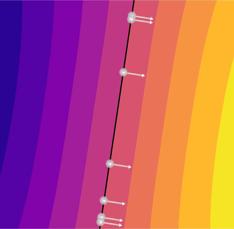
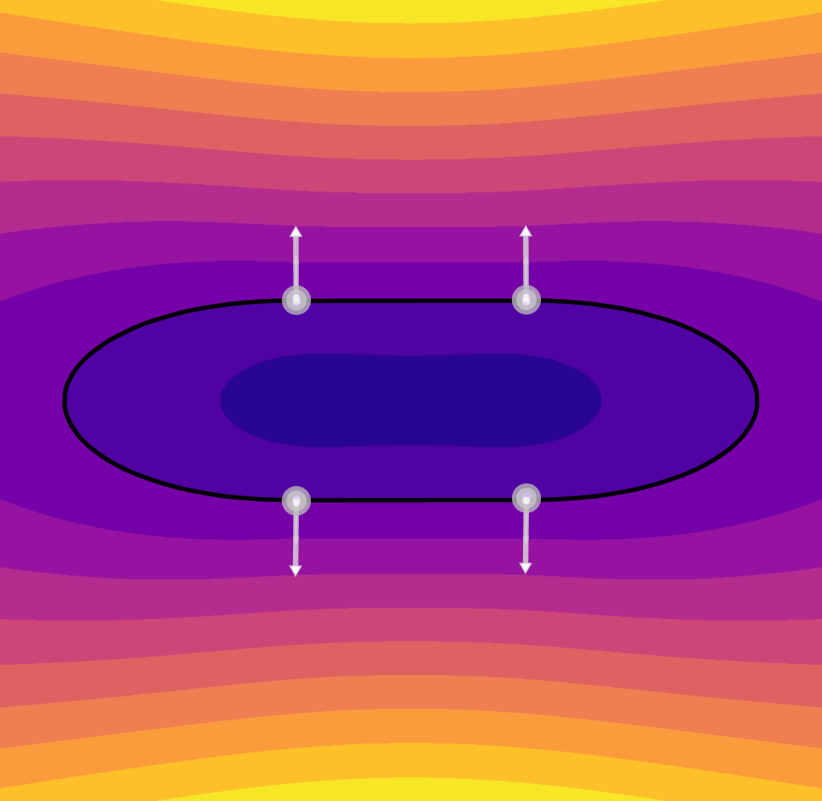
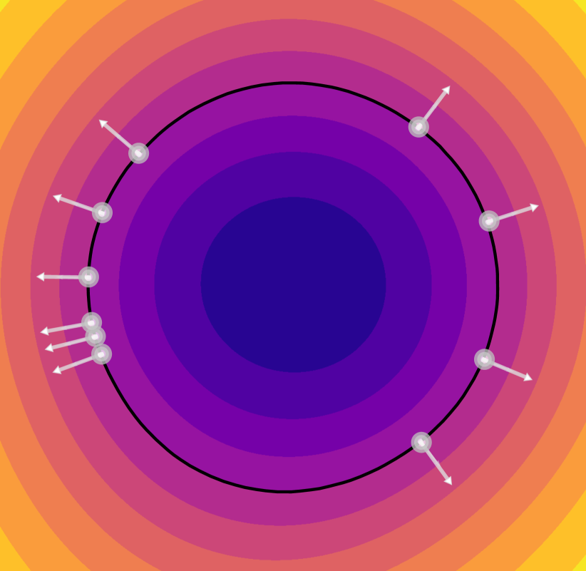
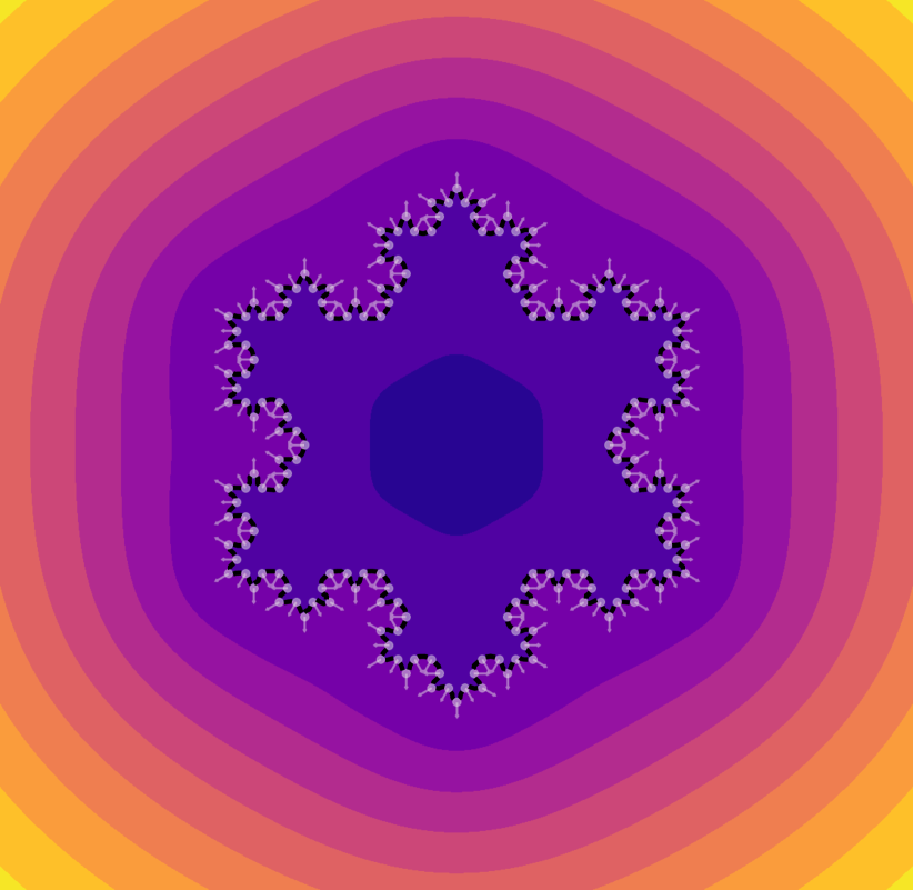
Estimating a 3D surface from a scattered point cloud is a classical and important problem in computer vision and computer graphics. In this task, the input is a set of 3D points sampled from an unknown surface and, possibly, normals of the surface at those points. The goal is to estimate a representation of the complete surface from which the input samples were obtained, for example, a polygonal mesh or an implicit function. This problem is challenging in practice: It is inherently ill-posed, since an infinite number of surfaces can interpolate the data. Furthermore, the input 3D points are often incomplete and noisy, as they are acquired from range sensors such as LIDAR, structured light, and laser scans. Ideally, the recovered surface should not interpolate noise but preserve key features and surface details.
Many early surface reconstruction techniques consider a kernel formulation of the surface reconstruction problem, using translation-invariant kernels such as biharmonic RBFs [9], Gaussian kernels [22], or compactly supported RBFs [34]. Currently, the most widely used method for surface reconstruction is Screened Poisson Surface Reconstruction [31], which solves a variant of the Poisson equation to find an implicit function whose zero-level set produces an approximating surface. We show in this paper that this method can also be viewed as a kernel method for a particular choice of kernel.
More recently, many papers have used neural networks to represent an implicit function or a local chart in a manifold atlas as a means of reconstructing a surface [44, 19, 26, 3, 24, 40, 42]. These methods can be integrated into a data-driven learning pipeline or directly applied in the so called “overfitting” regime, where a massively overparameterized (\ie, more parameters than input points) neural network is fitted to a single input point cloud as a functional representation for a surface. Empirical evidence has shown that these methods enjoy some form of “implicit regularization” that biases the recovered surface towards smoothness. Moreover, employing early stopping in gradient descent can prevent these approaches from interpolating noise.
Under certain parameter initializations, infinitely-wide neural networks de facto behave as kernel machines [30, 14], defining Reproducing Kernel Hilbert Spaces (RKHS), whose kernel is obtained by linearizing the neural network mapping around its initialization. While the kernel regime simplifies non-linear neural network learning into a convex program and provides a simple explanation for the successful optimization of overparameterized models, it cannot explain the good generalization properties observed for high-dimensional problems due to the inability of the RKHS to approximate non-smooth functions [4]. However, the situation for low-dimensional problems such as surface reconstruction is entirely different, and RKHS can provide powerful characterizations of regularity. In this context, [45] shows that in the univariate case the RKHS norm associated with a wide ReLU network is a weighted curvature, and leads to cubic spline interpolants. In higher dimensions, similar (albeit more complex) characterizations of the RKHS norm exist [35] (see also Proposition 2). In order to assess the benefits of neural networks on such low-dimensional problems, it is thus important to first understand their linearized counterparts, given by their associated kernel machines.
In this work, we demonstrate that in fact kernels arising from shallow ReLU networks are extremely competitive for 3D surface reconstruction, achieving state-of-the-art results: outperforming classical methods as well as non-linear methods based on far more complex neural network optimization.
Kernels provide many advantages over neural networks in our context: (i) They are well understood theoretically. (ii) Kernel regression boils down to solving a linear system, and avoids gradient descent that suffers from slow convergence. (iii) Kernel-based interpolants are represented using a number of parameters that is linear in the size of the input, whereas overparameterized neural networks require many more parameters than points. (iv) The inductive bias of kernel methods can be characterized explicitly via the RKHS norm (Section 3.3). (v) Kernel methods lend to scalable and efficient implementations (Section 3.5). We provide explicit expressions for two kinds of infinite-width ReLU kernels, their derivatives, and their corresponding RKHS norms. We further argue that these kernels can be viewed as a multidimensional generalization of cubic spline interpolation in 1D. Moreover, we show that Poisson Surface Reconstruction can itself be viewed as a kernel method and give an expression for its RKHS norm, suggesting that kernels are a broad framework which enable the rigorous understanding both traditional and modern surface reconstruction techniques.
1.1 Additional Related Work
Methods for 3D surface reconstruction can mostly be divided by their choice of surface representation: These are (i) the zero level set of a volumetric scalar function [31, 3, 24, 33, 36, 10, 40, 42], (ii) the fixed point of a projection operator onto locally fitted patches [1, 25, 29], (iii) a mesh connecting the input points [28], (iv) a collection of local parametric maps [44, 26, 17, 19], or (v) the union of parametric shapes [21, 20, 16, 13, 43]. For a recent up-to-date survey of surface reconstruction techniques, we refer the reader to [6].
The “random feature” kernels used this paper arise from training the top-layer weights in two-layer networks of infinite width and were described in [15, 32]. More recently, a lot of work has focused on a different kernel, known as the “neural tangent kernel” [30, 14], that linearly approximates the training of both layers of a neural network. We chose to use random feature kernels since, when the input dimension is small, typical initializations in neural networks lead to mainly training the top layer weights. More broadly, the function spaces associated with shallow neural networks were studied in [4, 7, 35, 39, 45].
2 Neural Spline Formulation
We formulate the problem of surface reconstruction as the task of finding a scalar function whose zero level set is the estimated surface (see Figure 1). In its most general form in arbitrary dimensions, we write our problem as follows.
We assume we are given a set of input points , function values , and normals . Our goal is to optimize an objective function of the form:
| (1) |
Here is a family of functions parameterized by . For surface reconstruction, we have and , since the reconstructed surface is given by the zero level set.
We begin by introducing the Neural Spline family of functions through the lens of finite-width shallow neural networks in Section 2.1, and turn to the infinite-width limit formulation in Section 2.2. While our approach is simple and our derivations straightforward, we differ slightly from a standard kernel regression setting since we employ a multi-dimensional kernel that includes the gradient of the fitted function. This formulation allows us to fit points and normals simultaneously.
2.1 Finite-Width Kernel
We first assume that the model is a two-layer ReLU neural network with neurons, but we keep the bottom layer weights fixed from initialization:
| (2) |
Here we write for the ReLU function. The bottom-layer weights are fixed randomly according to some specified distribution.
Remark 1.
In typical initialization schemes for neural networks (\eg, Kaiming He initalization [27]), the weights of each layer are initialized with a variance that is inversely proportional to the number of inputs of that layer. Our choice of fixing is motivated by the fact that using a standard two-layer network, for a given target model and as , only the top layer weights tend to vary throughout training [45].
Our model (2) is linear in the parameters , so our objective function is convex. However, since we assume , we expect to have an infinite set of global minimizers (an affine subspace in . Our goal is to find the minimizer with smallest parameter norm:
This minimizer is given explicitly by where denotes the Moore-Penrose pseudo-inverse of and
| (3) |
so that and . If has full rank, then and we can equivalently look for such that where . Note that can be viewed as a Gram matrix associated with the multi-dimensional kernel described by
| (4) |
where for compactness we used , and .
2.2 Infinite-Width Kernel
As the number of neurons tends to infinity, the kernel (4) converges to defined by
| (5) |
where is the chosen distribution of bottom layer weights . We use this kernel to characterize the interpolant in the infinite-width limit. For this, we simply replace in (4) with and solve the linear system the described in the previous section. More concretely (and rearranging terms), our goal is to recover such that
| (6) |
Our interpolant is such that for all . It can also be viewed as the solution to
| (7) | ||||
where is the RKHS corresponding to the one-dimensional kernel . In Section 3.3 we give an expression for the norm that defines the inductive bias of solutions. In Appendix B, we provide analytic expressions for the kernel (5) for two natural distributions over the weights :
| Uniform: | (8) | |||
| Gaussian: | (9) |
The uniform distribution (8) corresponds to the default initialization of linear layers in PyTorch and, as we argue in Section 3.1, it leads to a direct generalization of cubic spline interpolation. However, the Gaussian initialization actually leads to simpler analytical expressions for and produces almost the same results. We refer to Appendix B for a discussion and comparison of the two distributions.
3 Discussion
3.1 Connection to Cubic Splines in 1D
When , the uniform initialization (8) is such that and, assuming , the top-left element in is given by
| (10) | ||||
The expression assuming is obtained by swapping and . For fixed , the map is piecewise cubic and twice continuously differentiable (). This implies that kernel regression with (10) yields cubic spline interpolation. Applying the Neural Spline objective (1) with derivative constraints at the samples in also yields a piecewice cubic interpolant, although this curve is in general only . For other distributions of and , the kernel is no longer cubic, but the norm in the RKHS is a weighed norm of curvature (see [45] for details). In this sense, our approach with the initialization (8) can be viewed as a multi-dimensional version of spline interpolation.
3.2 Regularization and Robustness to Noise
To deal with noisy data, we can optionally add a simple regularizer term to our formulation that corresponds to penalizing the RKHS norm of the interpolant (“kernel ridge regression”). Concretely, we replace (6) with
| (11) |
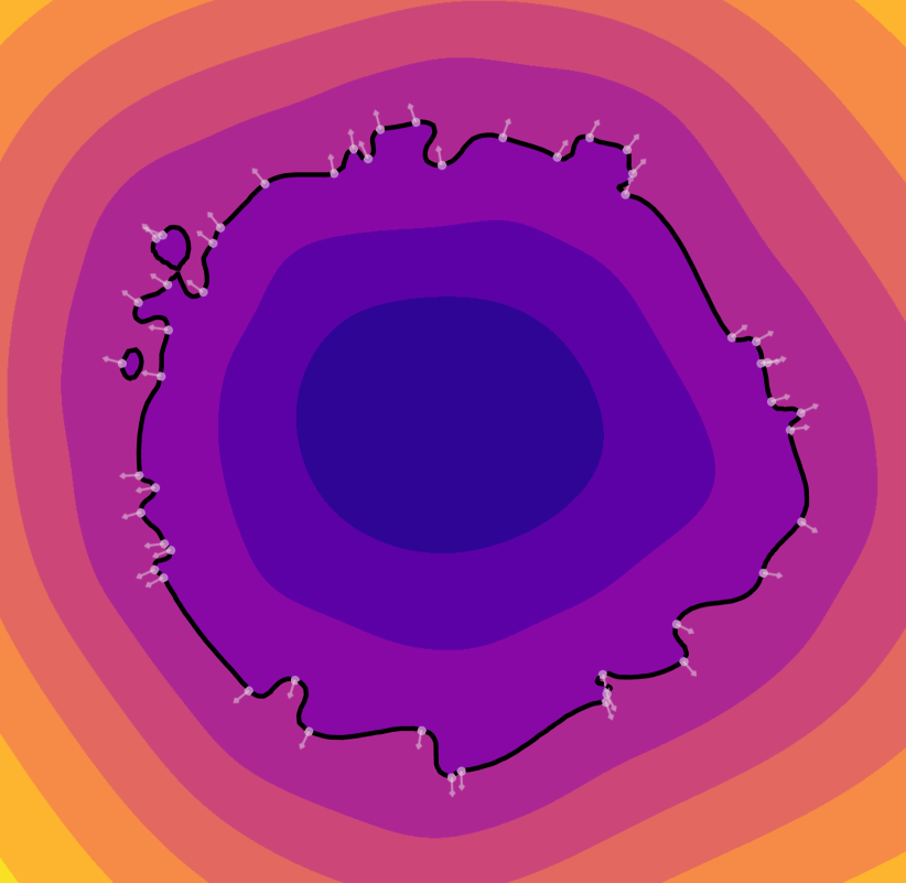
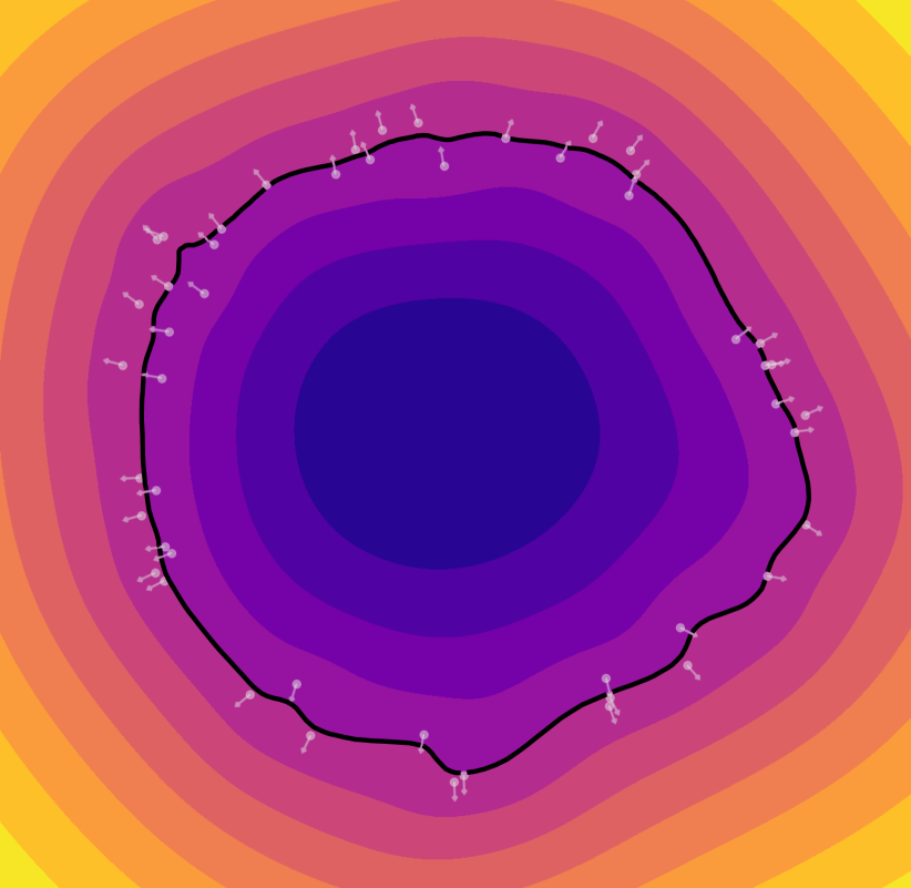
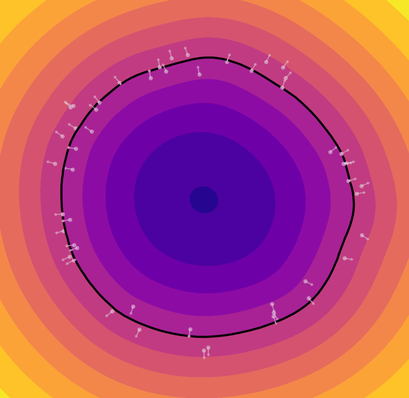
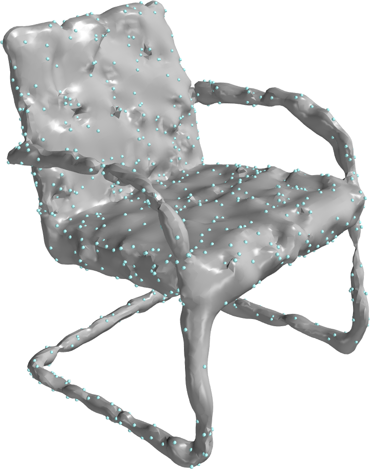
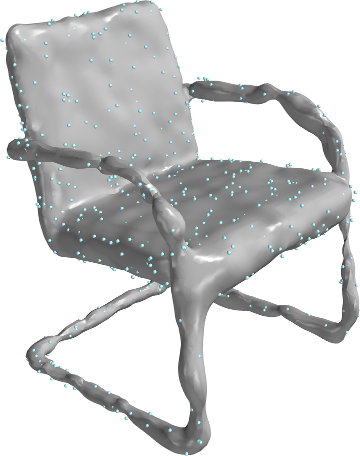
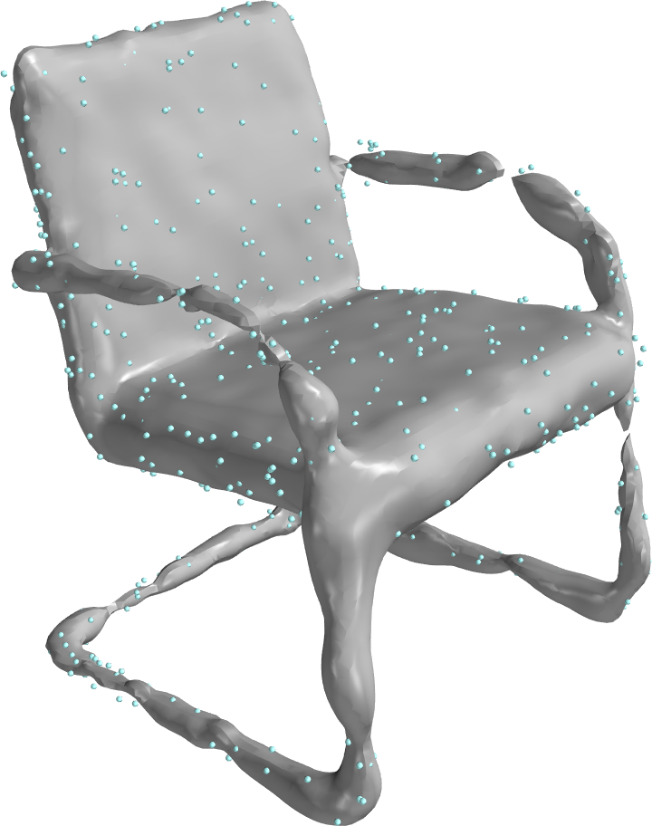
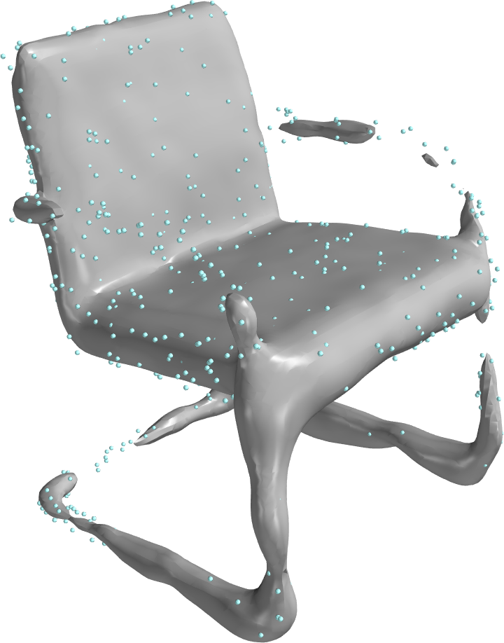
for . The regularizer term affects the spectrum of the Gram matrix by smoothing its smallest eigenvalues, with a similar effect to early stopping in gradient descent (see \eg [2]). Figure 2 shows examples of applying this regularizer on 2D and 3D problems.
3.3 Inductive Bias of Interpolants
Our interpolant belongs to the Hilbert space given by
| (12) |
where is a measure over the weights (\eg, (8) or (9)), and can be viewed as a continuous analog of the outer-layer weights of the finite network given by (2). The inductive bias of Neural Splines is thus determined by the RKHS norm in (12) since our method outputs the interpolating function which minimizes that norm. As noted in [35], if and then, by differentiating twice, we note that the Laplacian of is given by
| (13) |
By comparing (12) and (13), we see that the RKHS norm and the Laplacian of are closely related. More precisely, the Laplacian is the Dual Radon Transform of . Under certain assumptions, (13) can be inverted, yielding an explicit expression for in terms of . Intuitively, this shows that bounding the RKHS norm imposes a constraint on the Laplacian of , and thus encourages to be smooth. We report the following statement from [35] and we refer to Appendix D for more details.
Proposition 2.
3.4 Poisson Surface Reconstruction as a Kernel
We cast Screened Poisson Surface Reconstruction [31] in kernel form to facilitate comparisons. In its simplest form, Poisson reconstruction, extracts the level set of a smoothed indicator function determined as the solution of
where is a vector field obtained from normals at samples , and we use to denote the (smoothed) indicator function as it plays the same role as in (1). The equation above is closely related to (1): specifically, it is the equation for the minimizer of and the second term in (1) can be viewed as a approximation of this term by sampling at . The screened form of Poisson reconstruction effectively adds the first term with , as the indicator function at points of interest is supposed to be zero. For the Poisson equation, the solution can be explicitly written as an integral
The vector field is obtained by interpolating the normals using a fixed-grid spline basis and barycentric coordinates of the sample points with respect to the grid cell containing it. This is equivalent to using a non-translation invariant non-symmetric locally-supported kernel :
Lemma 3.
Let be a set of points arranged on a regular grid, be the trilinear basis function, and be a degree- spline basis function (See Appendix C for equations for and ). The kernel corresponding to Poisson Surface Reconstruction is
| (14) |
where .
To study the qualitative properties of this kernel, we replace with a radial kernel (see Appendix C) which has qualitatively similar behavior (see Figure 3). Since both and the Laplace kernel are radial functions, their convolution is also radial, yielding a translation-invariant radial approximation of :
| (15) |
Lemma 4.
The RKHS norm of the corresponding to the approximate Poisson kernel is
| (16) |
where is the Fourier transform.
We discuss the kernel formulation of Poisson Reconstruction in more detail in Appendix C.
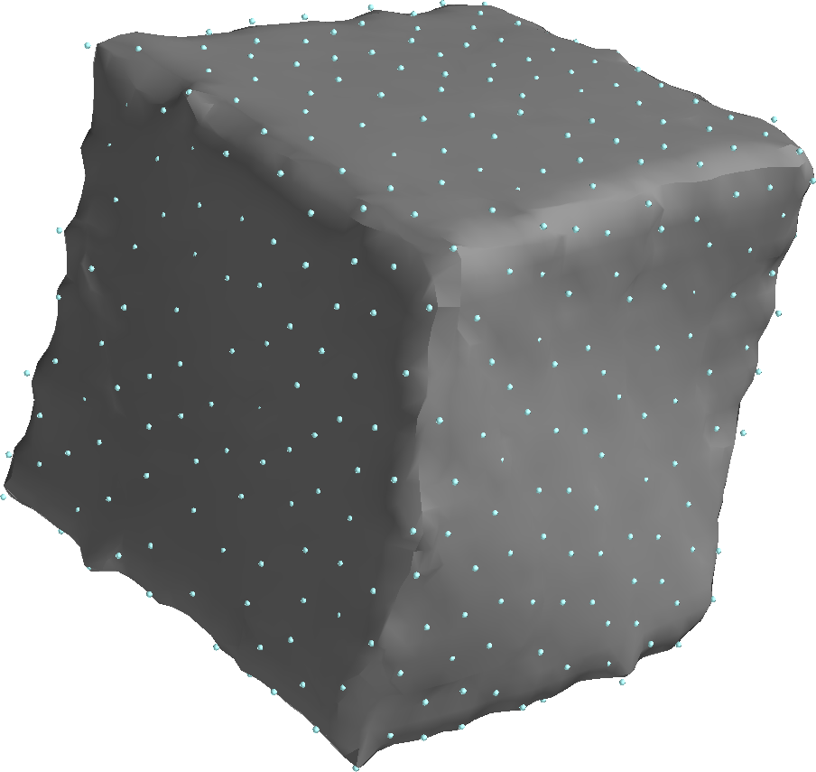
Approximate Poisson Kernel
Poisson Surface Reconstruction
3.5 Fast and Scalable Implementation
We provide a fast and scalable implementation of Neural Spline kernels based on FALKON [38], a recently-proposed solver for kernel-ridge-regression which runs in parallel on the GPU. While naïve kernel ridge-regression with points requires solving and storing an dense linear system, FALKON uses conjugate gradient descent requiring only storage, and convergence (though in practice we find that even for very large inputs, we converge in fewer than 10 iterations). To speed up convergence, FALKON can optionally store an preconditioner matrix in CPU memory (where , see paragrph below). To maximize performance and reduce memory overhead, we rely on KeOps [12] to evaluate kernel matrix-vector products symbolically on the GPU, which means our implementation uses only a small constant amount GPU memory and can be readily used on commodity hardware. Section 4.4 compares the performance of our implementation against other state of the art surface reconstruction techniques. We note that in principle, low-dimensional kernel methods can be accelerated using fast multipole-based approaches [23] (in particular, in the context of 3D surface reconstruction this was used in [9]); this yields optimal time complexity, for dense matrix-vector multiplication.
Nyström Subsampling
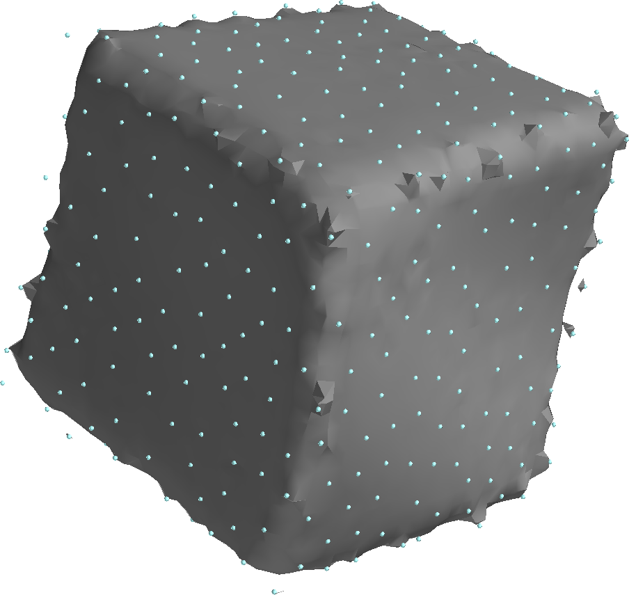
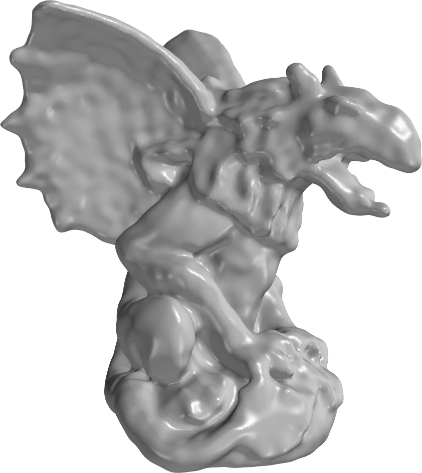
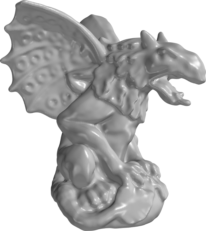
Full kernel ridge regression predicts a function which is supported on every input point as in (6), requiring coefficients to store the resulting function. We rely on Nyström sampling [18] to instead produce a kernel function which is supported on a small -sized subset of the input points (while still minimizing a loss on all the points). This is equivalent to approximating the kernel matrix with a low rank linear system. To choose Nyström samples, we leverage the geometric nature of our problem and select these by downsampling the input point cloud to have a blue-noise distribution using Bridson’s algorithm [8]. We demonstrate the effect of varying the number of Nyström samples qualitatively in Figure 4.


5k Nyström
10k Nyström
15k Nyström
75k Nyström
4 Experiments and Results
We now demonstrate the effectiveness of Neural Splines on the task of surface reconstruction. For all the experiments in this section, we used the analytical form of the kernel (5) with Gaussian initialization (8). Appendix A.7 compares the uniform (8) and Gaussian (9) kernels, showing almost no measurable difference in the reconstructions produced by either. We compare the empirical and analytical kernels in detail in Appendix A.6. An implementation of Neural Splines is available at https://github.com/fwilliams/neural-splines.
4.1 Sparse Reconstruction on Shapenet
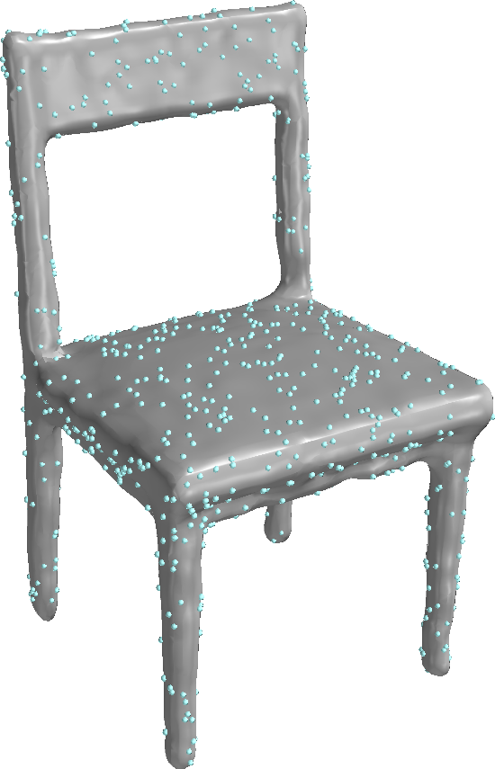
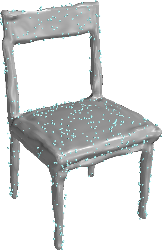
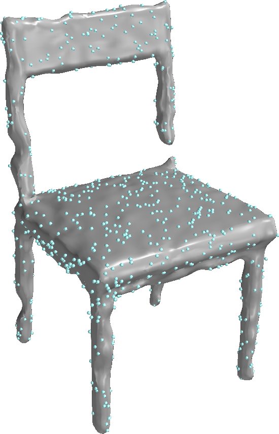
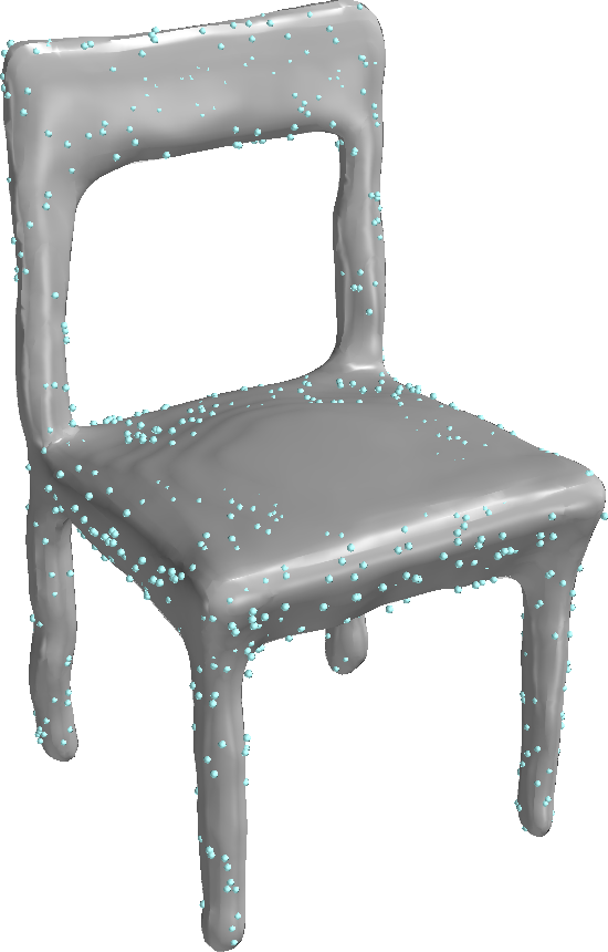
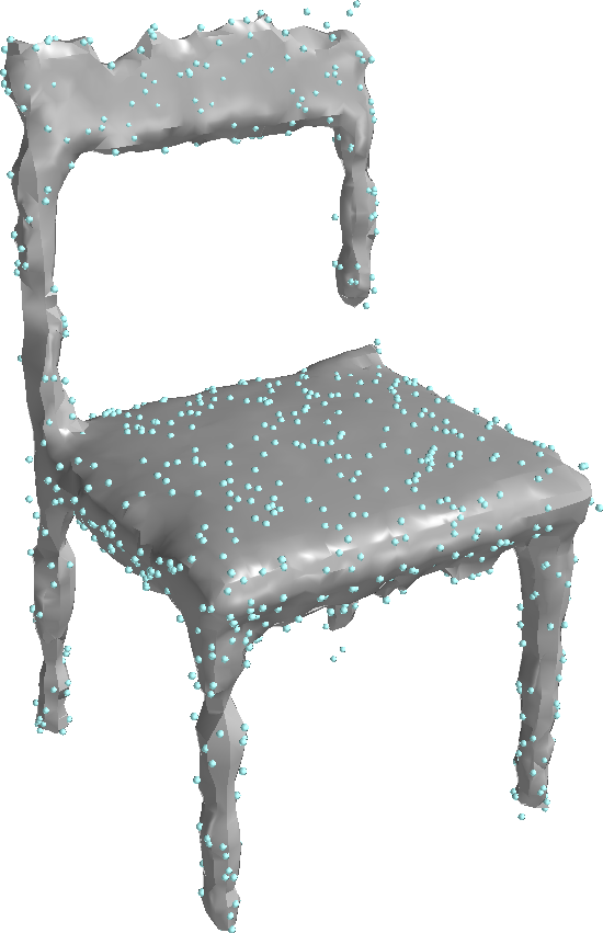
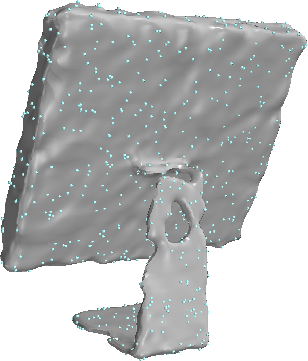
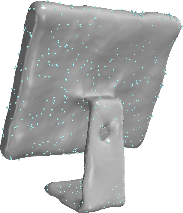
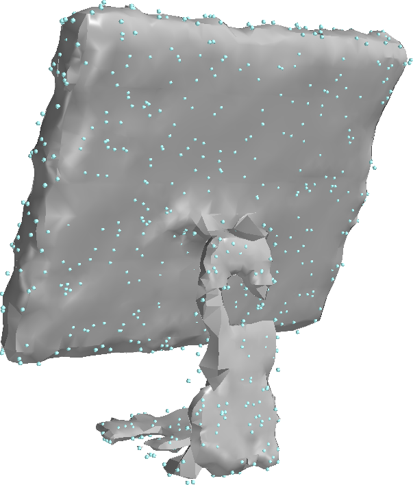
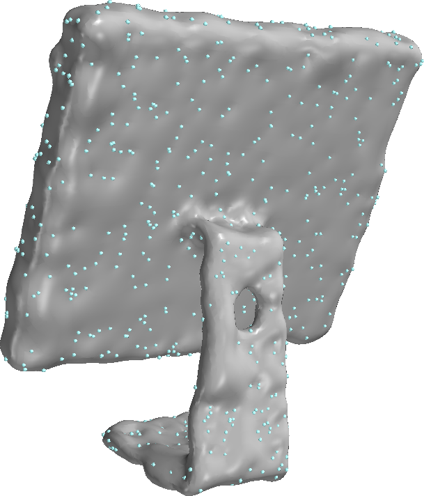
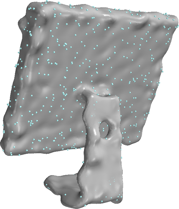
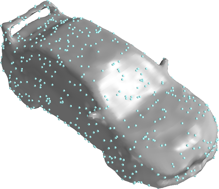
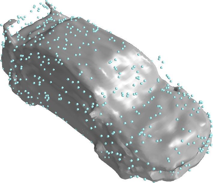
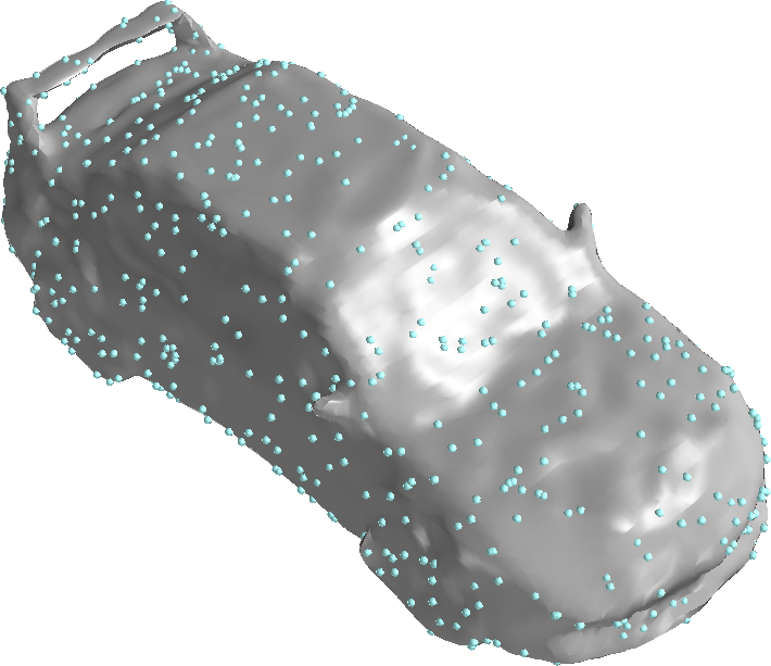
We performed a quantitative evaluation on a subset of the Shapenet dataset [11] to demonstrate that the inductive bias of Neural Splines is particularly effective for reconstructing surfaces from sparse points. We chose 1024 random points and normals sampled from the surface of 20 shapes per category across 13 categories (totalling 260 shapes). Using this dataset, we compared our method against Implicit Geometric Regularization (IGR) [24], SIREN [40], Fourier Feature Networks [42], Biharmonic RBF (Biharmonic) [9], SVM surface modelling (SVR) [22], and Screened Poisson Surface Reconstruction (Poisson) [31]. The first three techniques are modern neural network based methods, while the latter three techniques are classical methods based on kernels or solving a PDE. As criteria for the benchmark, we consider the Intersection over Union (IoU) and Chamfer Distance between the reconstructed shapes and the ground truth shapes. The former metric captures the accuracy of the predicted occupancy function, while the latter metric captures the accuracy of the predicted surface. Under both metrics, our method outperforms all other methods by a large margin. Table 1 reports quantitative results for the experiment and Figure 5 shows visual results on a few models. We report per-category results in Appendix A.4 and show many more figures in Appendix A.3.
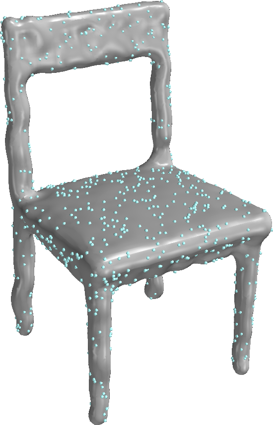
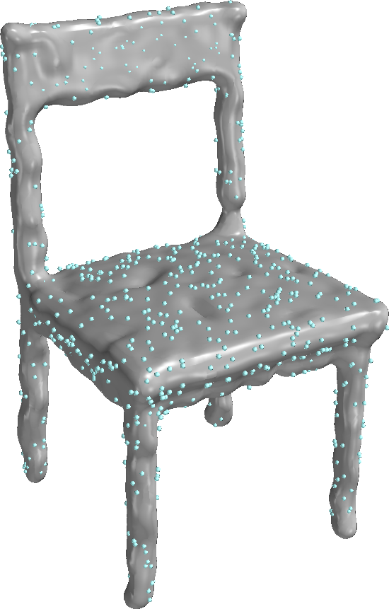
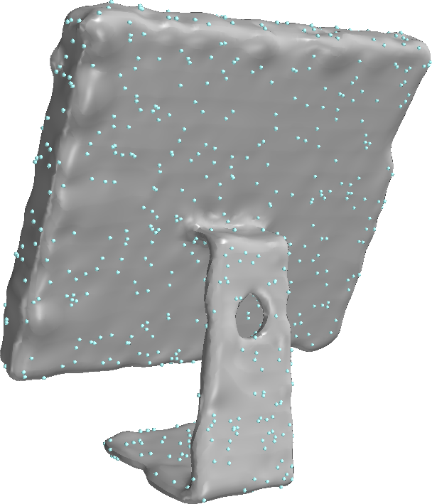
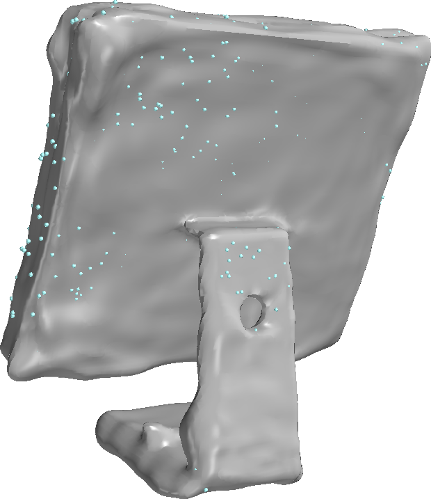
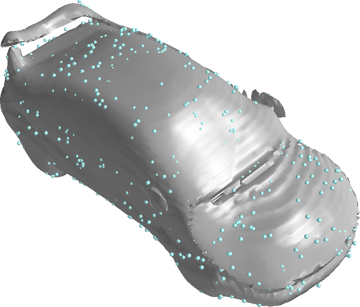
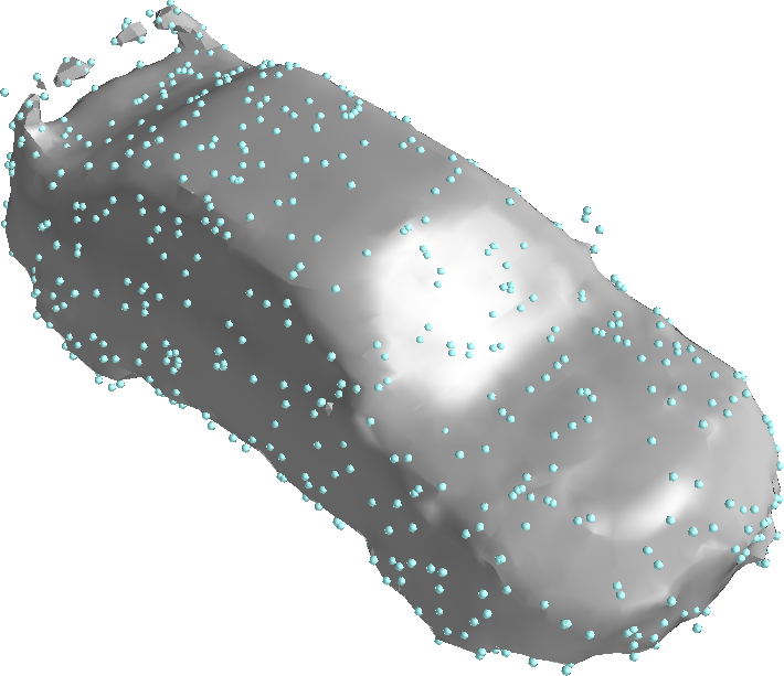
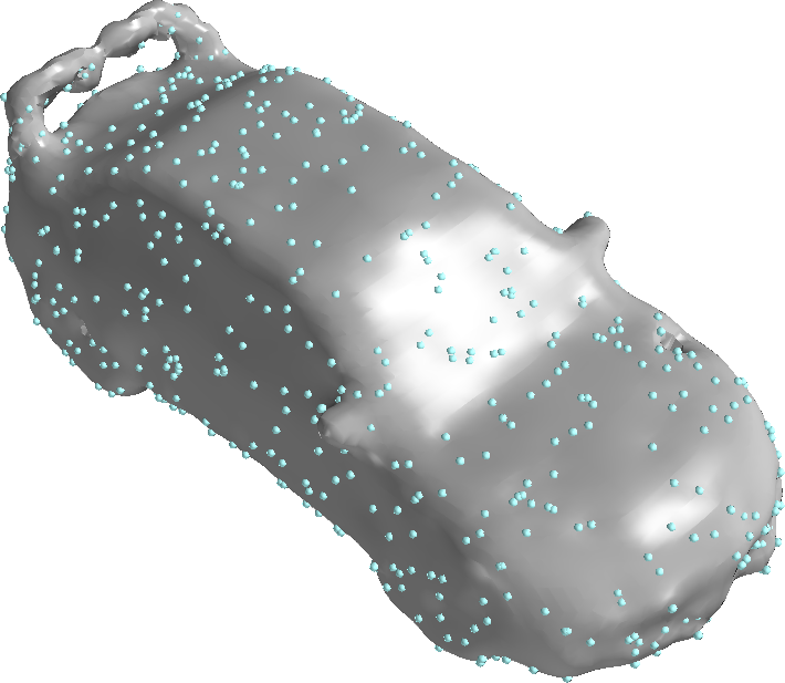
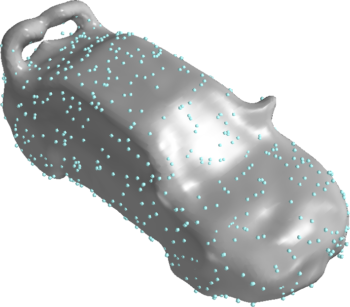
Ours
IGR
SIREN
Fourier Feats
Poisson
Biharmonic
SVR
| Method | mean | median | std | |
|---|---|---|---|---|
| IoU | Screened Poisson [31] | 0.6340 | 0.6728 | 0.1577 |
| IGR [24] | 0.8102 | 0.8480 | 0.1519 | |
| SIREN [40] | 0.8268 | 0.9097 | 0.2329 | |
| Fourier Feat. Nets [42] | 0.8218 | 0.8396 | 0.0989 | |
| Biharmonic RBF [9] | 0.8247 | 0.8642 | 0.1350 | |
| SVR [22] | 0.7625 | 0.7819 | 0.1300 | |
| Ours | 0.8973 | 0.9230 | 0.0871 | |
| Chamfer | Screened Poisson [31] | 2.22e-4 | 1.70e-4 | 1.76e-4 |
| IGR [24] | 5.12e-4 | 1.13e-4 | 2.15e-3 | |
| SIREN [40] | 1.03e-4 | 5.28e-5 | 1.93e-4 | |
| Fourier Feat. Nets [42] | 9.12e-5 | 8.65e-5 | 3.36e-5 | |
| Biharmonic RBF [9] | 1.11e-4 | 8.97e-5 | 7.06e-5 | |
| SVR [22] | 1.14e-4 | 1.04e-4 | 5.99e-5 | |
| Ours | 5.36e-5 | 4.06e-5 | 3.64e-5 |
Parameter Selection
Several of the above methods have parameters which can be tuned to increase performance. To ensure a fair comparison, we ran parameters sweeps for each Shapenet model for these methods, reporting the maximimum of each metric under consideration (see Appendix A.1 for a detailed description). For our method we did not tune parameters. We used no regularization and 1024 as Nyström samples for all models.
4.2 Surface Reconstruction Benchmark
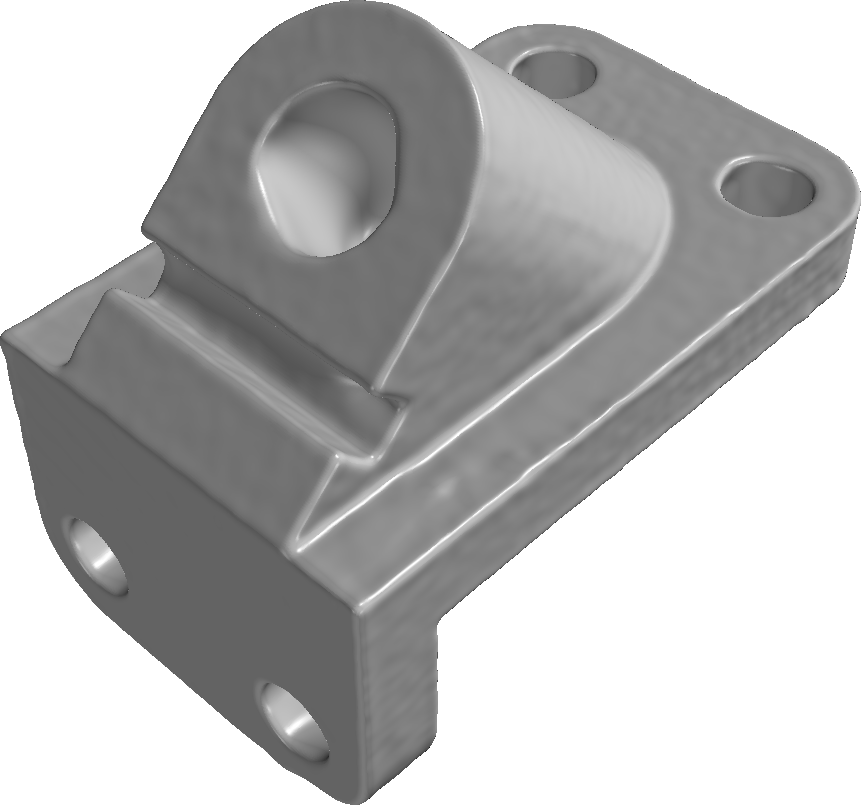
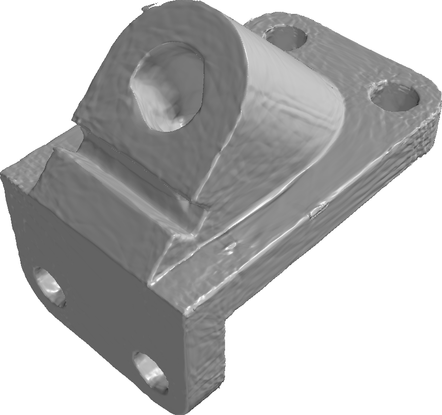
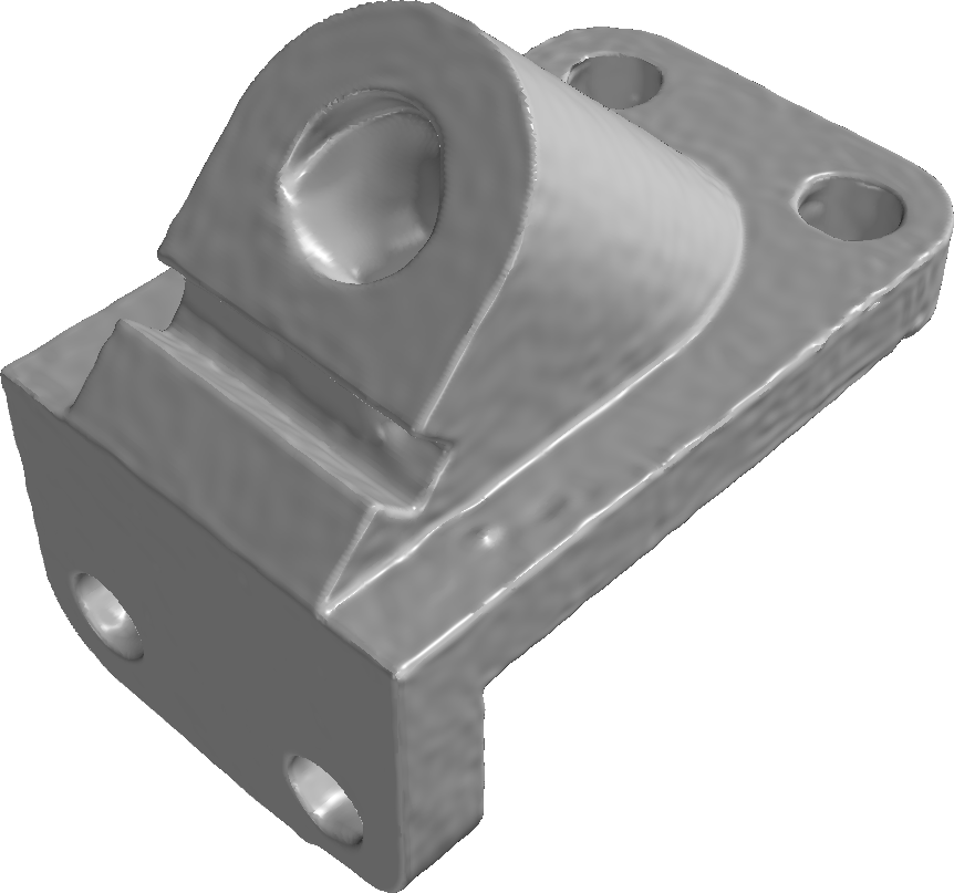
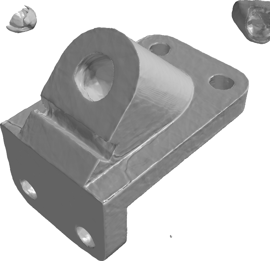
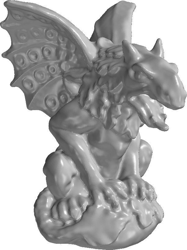
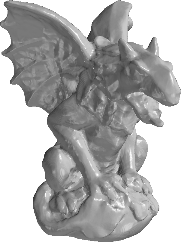
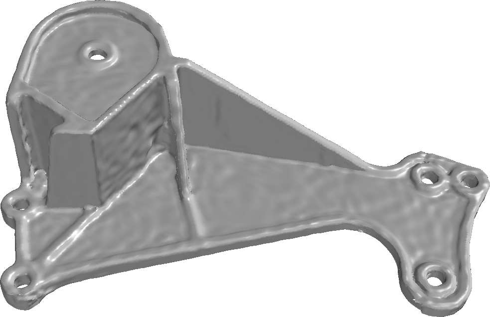
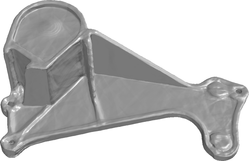
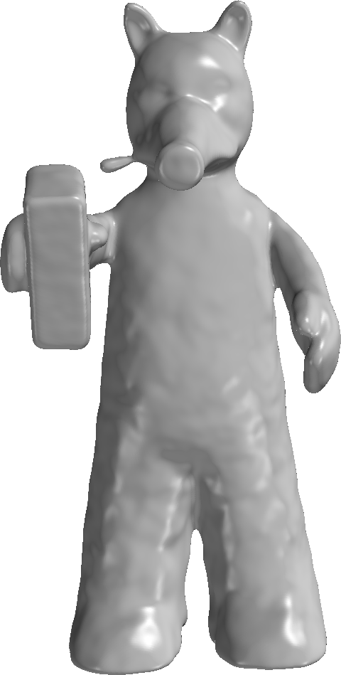
We evaluated our method on the Surface Reconstruction Benchmark [5] which consists of simulated noisy range scans (points and normals) taken from 5 shapes with challenging properties such as complex topologies, sharp features, and small surface details. We evaluate our method against Deep Geometric Prior (DGP) [44], Implicit Geometric Regularization (IGR) [24], SIREN [40], and Fourier Feature Networks (FFN) [42]. We remark that DGP establishes itself as superior to a dozen other classical methods on this benchmark and IGR furhter outperforms DGP. As in [24] and [44], Table 2 reports the Hausdorff () and Chamfer () distances between the reconstruction and ground-truth. We also report the one sided Hausdorff () and Chamfer () distances between the scan and the reconstruction, which measures how much the reconstructions overfits noise in the input. Our reconstructions are quantitatively closer to ground truth on all but one model. Figure 6 shows visual examples of a few models from the benchmark. All models are shown in Appendix A.3. As with the Shapenet benchmark, we did parameter sweeps for those methods which have tunable parameters, choosing the best model for each metric under consideration. See Appendix A.2 for details.

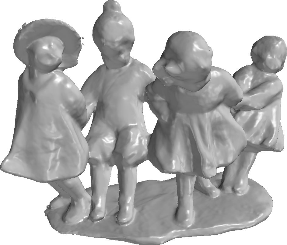
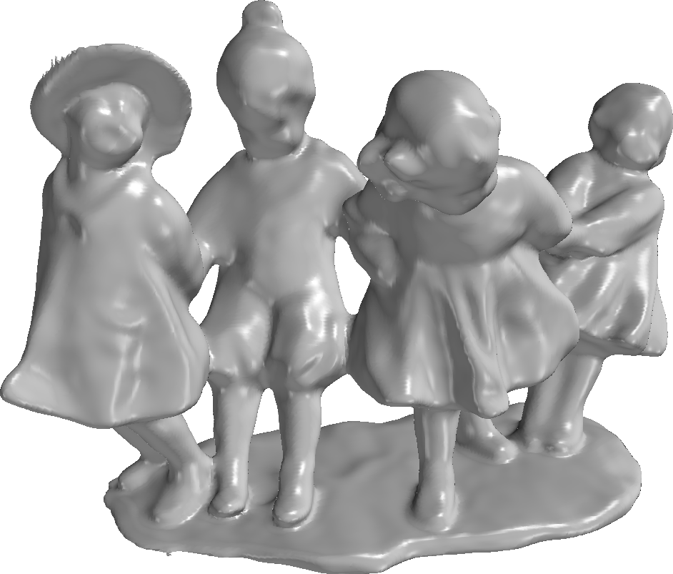
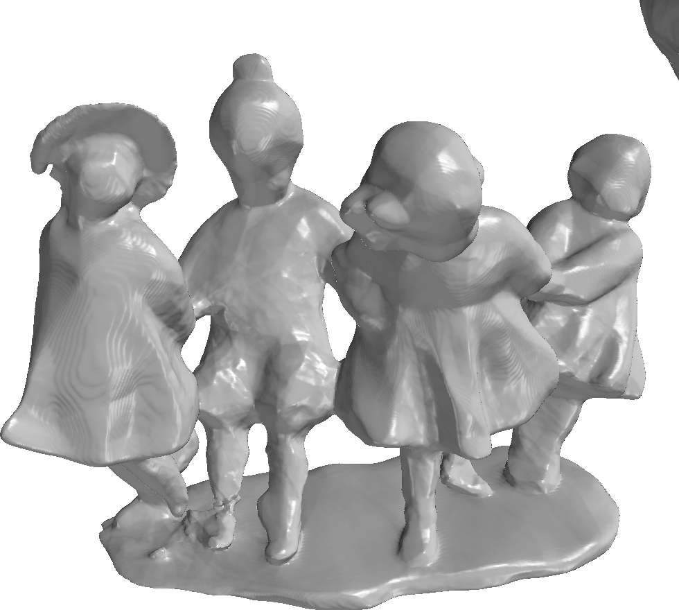

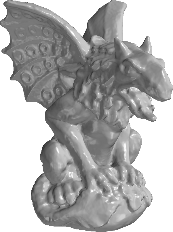
Ours
IGR
SIREN
Fourier Feats
| Ground Truth | Scans | ||||
|---|---|---|---|---|---|
| Method | |||||
| Anchor | DGP [44] | 0.33 | 8.82 | 0.08 | 2.79 |
| IGR [24] | 0.22 | 4.71 | 0.12 | 1.32 | |
| SIREN [40] | 0.32 | 8.19 | 0.11 | 2.43 | |
| FFN [42] | 0.31 | 4.49 | 0.10 | 0.10 | |
| Ours | 0.22 | 4.65 | 0.11 | 1.11 | |
| Daratech | DGP [44] | 0.2 | 3.14 | 0.04 | 1.89 |
| IGR [24] | 0.25 | 4.01 | 0.08 | 1.59 | |
| SIREN [40] | 0.21 | 4.30 | 0.09 | 1.77 | |
| FFN [42] | 0.34 | 5.97 | 0.10 | 0.10 | |
| Ours | 0.21 | 4.35 | 0.08 | 1.14 | |
| DC | DGP [44] | 0.18 | 4.31 | 0.04 | 2.53 |
| IGR [24] | 0.17 | 2.22 | 0.09 | 2.61 | |
| SIREN [40] | 0.15 | 2.18 | 0.06 | 2.76 | |
| FFN [42] | 0.20 | 2.87 | 0.10 | 0.12 | |
| Ours | 0.14 | 1.35 | 0.06 | 2.75 | |
| Gargoyle | DGP [44] | 0.21 | 5.98 | 0.06 | 3.41 |
| IGR [24] | 0.16 | 3.52 | 0.06 | 0.81 | |
| SIREN [40] | 0.17 | 4.64 | 0.08 | 0.91 | |
| FFN [42] | 0.22 | 5.04 | 0.09 | 0.09 | |
| Ours | 0.16 | 3.20 | 0.08 | 2.75 | |
| Lord Quas | DGP [44] | 0.14 | 3.67 | 0.04 | 2.03 |
| IGR [24] | 0.12 | 1.17 | 0.07 | 0.98 | |
| SIREN [40] | 0.17 | 0.82 | 0.12 | 0.76 | |
| FFN [42] | 0.35 | 3.90 | 0.06 | 0.06 | |
| Ours | 0.12 | 0.69 | 0.05 | 0.62 | |
4.3 Large Scale Reconstruction of Full Scenes
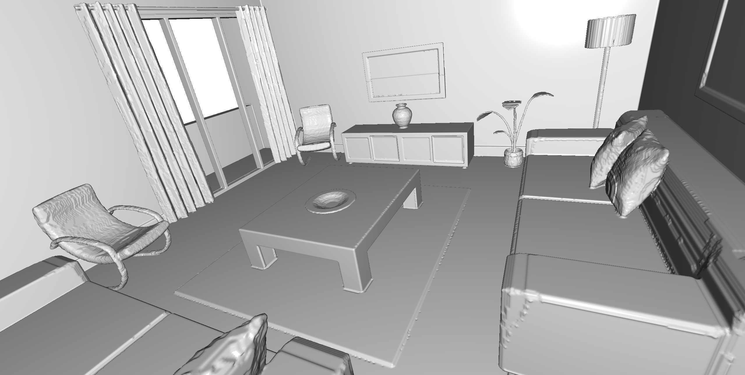
Figure 7 shows a full scene consisting of 9 million points reconstructed using our method. This is the same scene used in [40], and contains many thin features that are difficult to reconstruct (\eg, curtains, plant, and lampshade). To generate the input point cloud for this experiment, we densely sampled a mesh extracted from a occupancy grid of the scene. To perform the reconstruction, we subdivided the space into 8x8x8 cells containing between 10k and 500k samples and reconstructed each cell interdependently using up to 15k Nyström samples. The whole process takes 1.5 hours on a machine with an NVIDIA 1080Ti GPU.
4.4 Timing and Performance
Table 3 compares the average running time and GPU memory usage of our method and others when reconstructing point clouds from the Surface Reconstruction Benchmark described in Section 4.2. To ensure a fair comparison we ran all neural network based methods for 5000 iterations. We do not report exact CPU memory usage for the methods since it is hard to measure but we remark that, by observation, system memory usage never exceeded 3GiB for any of the methods. Appendix A.5 reports the running times and memory usages for individual models in the benchmark.
| FFN | IGR | SIREN | Poisson | Ours | |
| Runtime (sec) | 337.71 | 1413.94 | 599.00 | 1.64 | 11.91 |
| Max VRAM (MiB) | 3711 | 5093 | 1607 | N.A. | 5285 |
4.5 Our Method versus Neural Networks
5k Iter
50k Iter
75k Iter
100k Iter
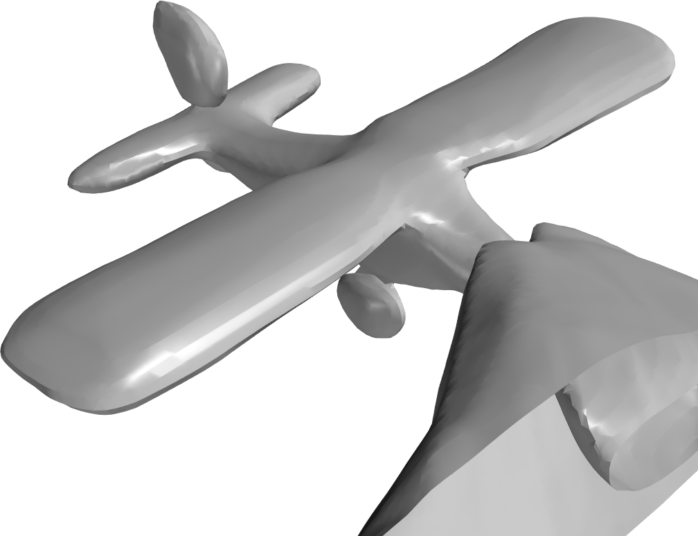
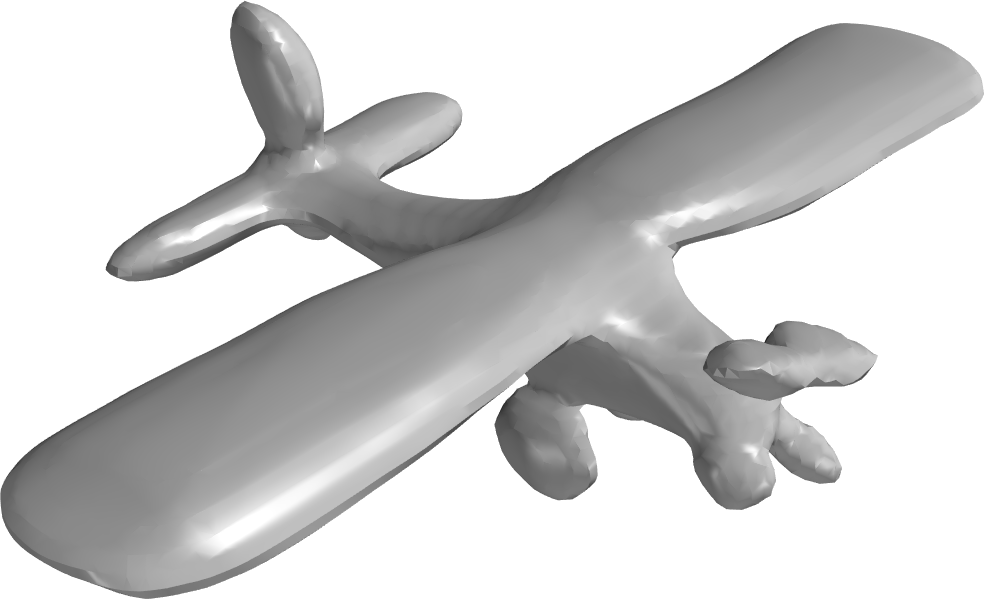
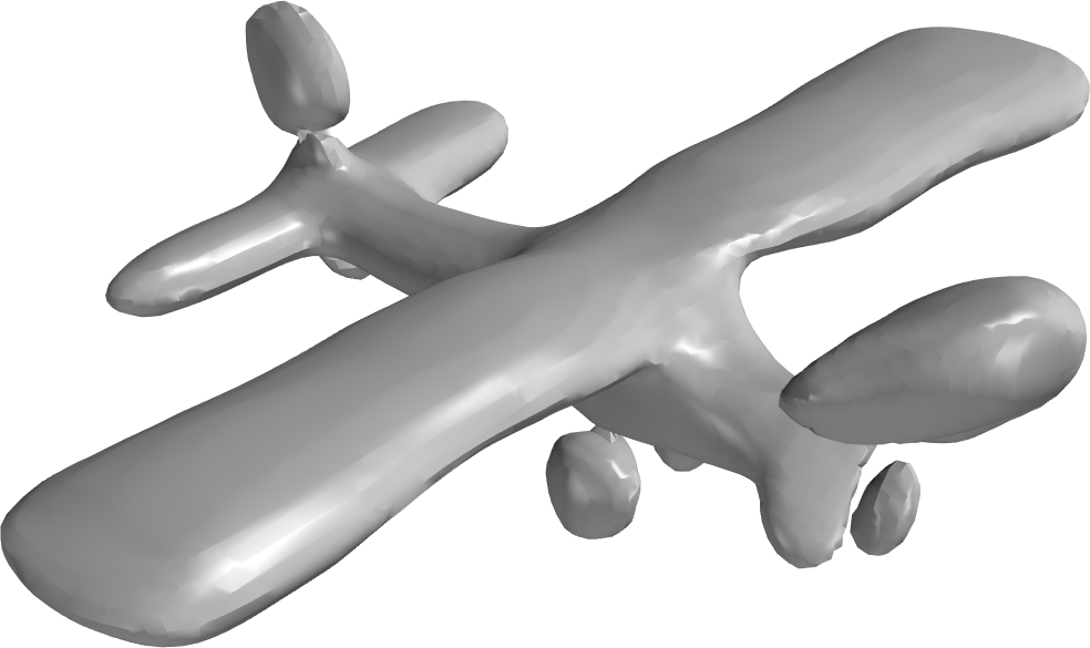
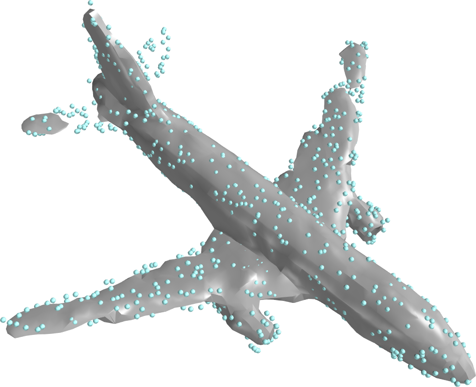
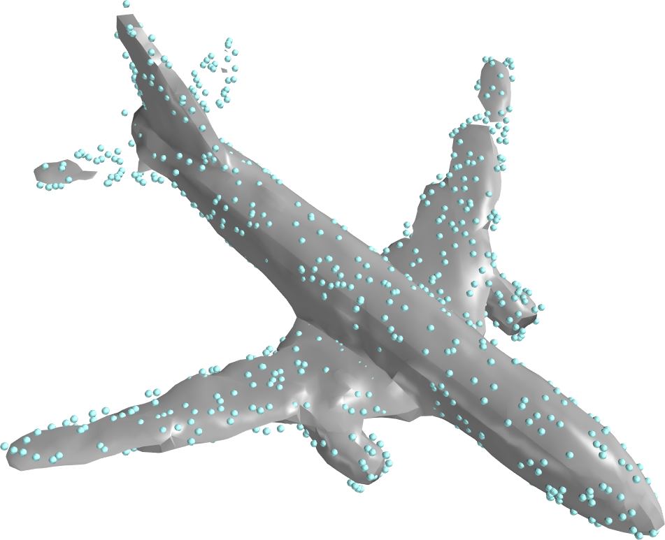
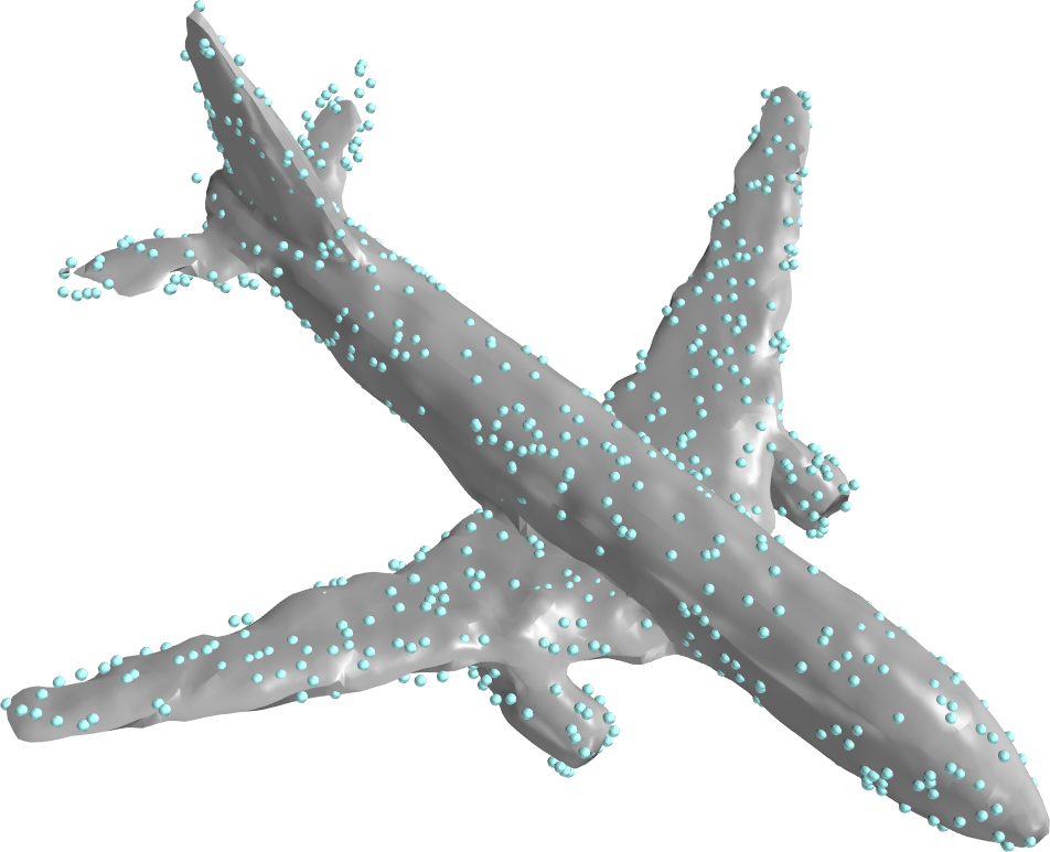
Implicit Geometric Regularization [24] demonstrates that ReLU networks have a natural inductive bias making them good at reconstructing shapes. However, methods based on ReLU networks suffer from slow convergence (see Figure 8). SIREN [40] drastically improves convergence speed by replacing ReLU with sinusoidal activations and a clever initialization, however, SIREN occasionally underfits on sparse inputs and requires an additional loss computed on points in the volume around the shape to prevent reconstruction artefacts. This loss increase runtimes, and suggest that SIREN’s inductive bias may not be ideal for sparse reconstruction tasks. By projecting input points onto random Fourier features, Fourier Feature Networks (FFNs) [42] present a principled approach rooted in Kernel methods to control the inductive bias of the solution as well as convergence speed. While FFNs are capable of producing high quality solutions, they are sensitive to the choice of feature distribution when data is sparse (see Figure 9) and thus require tuning to work well. In contrast, our technique converges in seconds (Section 4.4), has a well suited inductive bias for shape representation (Section 3.3), and requires minimal parameter tuning.
5 Conclusion and Future Work
We have shown that Neural Spline kernels arising from infinitely wide shallow ReLU networks are very effective tools for 3D surface reconstruction, outperforming state-of-the-art methods while being computationally efficient and conceptually simple. In a sense, our work bridges the gap between traditional reconstruction methods and modern neural network based methods by leveraging the deep connection between neural networks and kernels.
We remark that our kernel formulation is fully differentiable. In the future, we hope to integrate Neural Splines into deep learning pipelines and apply them to other 3D tasks such as shape completion and sparse reconstruction. On the theory side, we would like to investigate and compare the approximation properties of different kernels (in particular those arising from infinite width sinusoidal networks) in the context of 3D reconstruction.
Acknowledgements
This work is partially supported by the Alfred P. Sloan Foundation, NSF RI-1816753, NSF CAREER CIF 1845360, NSF CHS-1901091, and Samsung Electronics.
References
- [1] Anders Adamson and Marc Alexa. Approximating and intersecting surfaces from points. In Proceedings of the 2003 Eurographics/ACM SIGGRAPH symposium on Geometry processing, pages 230–239. Eurographics Association, 2003.
- [2] Alnur Ali, J. Zico Kolter, and Ryan J. Tibshirani. A Continuous-Time View of Early Stopping for Least Squares. arXiv:1810.10082 [cs, stat], Feb. 2019.
- [3] Matan Atzmon and Yaron Lipman. Sal: Sign agnostic learning of shapes from raw data, 2019.
- [4] Francis Bach. Breaking the curse of dimensionality with convex neural networks. Journal of Machine Learning Research, 18(19):1–53, 2017.
- [5] Matthew Berger, Joshua A Levine, Luis Gustavo Nonato, Gabriel Taubin, and Claudio T Silva. A benchmark for surface reconstruction. ACM Transactions on Graphics (TOG), 32(2):1–17, 2013.
- [6] Matthew Berger, Andrea Tagliasacchi, Lee M Seversky, Pierre Alliez, Gael Guennebaud, Joshua A Levine, Andrei Sharf, and Claudio T Silva. A survey of surface reconstruction from point clouds. In Computer Graphics Forum, volume 36, pages 301–329. Wiley Online Library, 2017.
- [7] Alberto Bietti and Julien Mairal. On the Inductive Bias of Neural Tangent Kernels. arXiv:1905.12173 [cs, stat], Oct. 2019.
- [8] Robert Bridson. Fast poisson disk sampling in arbitrary dimensions. In ACM SIGGRAPH 2007 Sketches, SIGGRAPH ’07, page 22–es, New York, NY, USA, 2007. Association for Computing Machinery.
- [9] Jonathan C Carr, Richard K Beatson, Jon B Cherrie, Tim J Mitchell, W Richard Fright, Bruce C McCallum, and Tim R Evans. Reconstruction and representation of 3d objects with radial basis functions. In Proceedings of the 28th annual conference on Computer graphics and interactive techniques, pages 67–76, 2001.
- [10] Rohan Chabra, Jan Eric Lenssen, Eddy Ilg, Tanner Schmidt, Julian Straub, Steven Lovegrove, and Richard Newcombe. Deep local shapes: Learning local sdf priors for detailed 3d reconstruction, 2020.
- [11] Angel X. Chang, Thomas Funkhouser, Leonidas Guibas, Pat Hanrahan, Qixing Huang, Zimo Li, Silvio Savarese, Manolis Savva, Shuran Song, Hao Su, Jianxiong Xiao, Li Yi, and Fisher Yu. Shapenet: An information-rich 3d model repository, 2015.
- [12] Benjamin Charlier, Jean Feydy, Joan Alexis Glaunès, François-David Collin, and Ghislain Durif. Kernel operations on the GPU, with autodiff, without memory overflows. arXiv preprint arXiv:2004.11127, 2020.
- [13] Zhiqin Chen, Andrea Tagliasacchi, and Hao Zhang. Bsp-net: Generating compact meshes via binary space partitioning, 2020.
- [14] Lenaic Chizat, Edouard Oyallon, and Francis Bach. On lazy training in differentiable programming. In Advances in Neural Information Processing Systems, pages 2933–2943, 2019.
- [15] Youngmin Cho and Lawrence K Saul. Kernel methods for deep learning. In Advances in neural information processing systems, pages 342–350, 2009.
- [16] Boyang Deng, Kyle Genova, Soroosh Yazdani, Sofien Bouaziz, Geoffrey Hinton, and Andrea Tagliasacchi. Cvxnet: Learnable convex decomposition, 2020.
- [17] Theo Deprelle, Thibault Groueix, Matthew Fisher, Vladimir G. Kim, Bryan C. Russell, and Mathieu Aubry. Learning elementary structures for 3d shape generation and matching, 2019.
- [18] Petros Drineas and Michael W Mahoney. On the nyström method for approximating a gram matrix for improved kernel-based learning. journal of machine learning research, 6(Dec):2153–2175, 2005.
- [19] Matheus Gadelha, Rui Wang, and Subhransu Maji. Deep manifold prior, 2020.
- [20] Kyle Genova, Forrester Cole, Avneesh Sud, Aaron Sarna, and Thomas Funkhouser. Local deep implicit functions for 3d shape, 2020.
- [21] Kyle Genova, Forrester Cole, Daniel Vlasic, Aaron Sarna, William T. Freeman, and Thomas Funkhouser. Learning shape templates with structured implicit functions, 2019.
- [22] Joachim Giesen, Simon Spalinger, and Bernhard Schölkopf. Kernel methods for implicit surface modeling. In L. K. Saul, Y. Weiss, and L. Bottou, editors, Advances in Neural Information Processing Systems 17, pages 1193–1200. MIT Press, 2005.
- [23] Leslie Greengard and Vladimir Rokhlin. A fast algorithm for particle simulations. Journal of computational physics, 73(2):325–348, 1987.
- [24] Amos Gropp, Lior Yariv, Niv Haim, Matan Atzmon, and Yaron Lipman. Implicit geometric regularization for learning shapes, 2020.
- [25] Gaël Guennebaud and Markus Gross. Algebraic point set surfaces. In ACM SIGGRAPH 2007 papers, pages 23–es. ACM New York, NY, USA, 2007.
- [26] Rana Hanocka, Gal Metzer, Raja Giryes, and Daniel Cohen-Or. Point2mesh: A self-prior for deformable meshes, 2020.
- [27] Kaiming He, Xiangyu Zhang, Shaoqing Ren, and Jian Sun. Delving deep into rectifiers: Surpassing human-level performance on imagenet classification. 2015 IEEE International Conference on Computer Vision (ICCV), Dec 2015.
- [28] Hugues Hoppe, Tony DeRose, Tom Duchamp, John McDonald, and Werner Stuetzle. Surface reconstruction from unorganized points. In Proceedings of the 19th annual conference on Computer graphics and interactive techniques, pages 71–78, 1992.
- [29] Hui Huang, Shihao Wu, Minglun Gong, Daniel Cohen-Or, Uri Ascher, and Hao Zhang. Edge-aware point set resampling. ACM transactions on graphics (TOG), 32(1):1–12, 2013.
- [30] Arthur Jacot, Franck Gabriel, and Clément Hongler. Neural tangent kernel: Convergence and generalization in neural networks, 2018.
- [31] Michael Kazhdan and Hugues Hoppe. Screened poisson surface reconstruction. ACM Transactions on Graphics (ToG), 32(3):1–13, 2013.
- [32] Nicolas Le Roux and Yoshua Bengio. Continuous neural networks. In Artificial Intelligence and Statistics, pages 404–411, 2007.
- [33] Lars Mescheder, Michael Oechsle, Michael Niemeyer, Sebastian Nowozin, and Andreas Geiger. Occupancy networks: Learning 3d reconstruction in function space. 2019 IEEE/CVF Conference on Computer Vision and Pattern Recognition (CVPR), Jun 2019.
- [34] Yutaka Ohtake, Alexander Belyaev, and Hans-Peter Seidel. Sparse surface reconstruction with adaptive partition of unity and radial basis functions. Graphical Models, 68(1):15–24, 2006.
- [35] Greg Ongie, Rebecca Willett, Daniel Soudry, and Nathan Srebro. A function space view of bounded norm infinite width relu nets: The multivariate case, 2019.
- [36] Jeong Joon Park, Peter Florence, Julian Straub, Richard Newcombe, and Steven Lovegrove. Deepsdf: Learning continuous signed distance functions for shape representation. 2019 IEEE/CVF Conference on Computer Vision and Pattern Recognition (CVPR), Jun 2019.
- [37] Alexander D Poularikas. Transforms and applications handbook. CRC press, 2018.
- [38] Alessandro Rudi, Luigi Carratino, and Lorenzo Rosasco. Falkon: An optimal large scale kernel method, 2018.
- [39] Pedro Savarese, Itay Evron, Daniel Soudry, and Nathan Srebro. How do infinite width bounded norm networks look in function space?, 2019.
- [40] Vincent Sitzmann, Julien N. P. Martel, Alexander W. Bergman, David B. Lindell, and Gordon Wetzstein. Implicit neural representations with periodic activation functions, 2020.
- [41] Donald C Solmon. Asymptotic formulas for the dual radon transform and applications. Mathematische Zeitschrift, 195(3):321–343, 1987.
- [42] Matthew Tancik, Pratul P. Srinivasan, Ben Mildenhall, Sara Fridovich-Keil, Nithin Raghavan, Utkarsh Singhal, Ravi Ramamoorthi, Jonathan T. Barron, and Ren Ng. Fourier features let networks learn high frequency functions in low dimensional domains, 2020.
- [43] Francis Williams, Jerome Parent-Levesque, Derek Nowrouzezahrai, Daniele Panozzo, Kwang Moo Yi, and Andrea Tagliasacchi. Voronoinet: General functional approximators with local support. In Proceedings of the IEEE/CVF Conference on Computer Vision and Pattern Recognition (CVPR) Workshops, June 2020.
- [44] Francis Williams, Teseo Schneider, Claudio Silva, Denis Zorin, Joan Bruna, and Daniele Panozzo. Deep geometric prior for surface reconstruction. 2019 IEEE/CVF Conference on Computer Vision and Pattern Recognition (CVPR), Jun 2019.
- [45] Francis Williams, Matthew Trager, Claudio Silva, Daniele Panozzo, Denis Zorin, and Joan Bruna. Gradient dynamics of shallow univariate relu networks, 2019.
Appendix A Additional Experiments
A.1 Detailed description of Shapenet Experiment
Many of the methods we compared against on Shapenet have tunable parameters which can drastically alter the quality of reconstructed outputs. To ensure a proper comparison, we ran sweeps over these parameters where appropriate choosing the best reconstruction for each model under both metrics (Chamfer and IoU). For our method we did no parameter sweeps, using no regularization and 1024 Nyström samples for each model in the dataset. We describe the exerimental methodology for each method in the benchmark below.
Implicit Geometric Regularization [24]
We trained each model for 5k iterations with Adam and a learning rate of 0.001 using the same parameters and architecture as proposed in the original paper. We included the normals in the loss with the parameter set to 1. The Eikonal regularization term was set to 0.1. While IGR can slightly improve by using a very large number of iterations. doing so is prohibitively slow over many models. Figure 8 motivates our choice of iterations, demonstrating only a slight improvements between 5k and 100k iterations (the latter which required 2 hours of fitting on a NVIDIA-1080-Ti GPU).
Screened Poisson Surface Reconstruction [31]
We considered every possible combination of the following parameters: the octree depth in , the number of points per leaf in , the point weight (which controls the degree to which the method interpolates the input) in . Since all the shapes in the benchmark are watertight meshes, we used Dirichlet boundary constraints for the reconstruction.
SIREN [40]
We trained used a SIREN network with 5 hidden layers each containing 256 neurons for 5000 iterations, using a learning rate of 1e-4 with Adam. We used the same loss for shapes as in the original SIREN paper, sampling an additional (where is the number of input points) points in an axis aligned bounding box whose diagonal is 10% larger than the object’s bounding box. We minimize the same loss for shapes as the SIREN paper (see section 4.2 in the original SIREN paper).
Fourier Feature Networks [42]
We used an 8-layer ReLU MLP with 256 Fourier features sampled from a Gaussian distribution. This is the same architecture as the shape representation experiment in the original paper. For each model in the benchmark, we did a parameter sweep on the variance of the Gaussian distribution, considering . The range of parameters was chosen by empirical verification on 3 models from the airplanes, benches, and cars categories.
SVR [22]
As in the original paper, we use a Gaussian kernel to perform support vector regression. To generate occupancy samples, we augmented the input points with an ”inside“ and ”outside“ point by perturbing them by along the normal at that point. We used forall the models. For each model we did a joint parameter sweep over the regularization parameter and the variance parameter . The range of parameters was chosen by empirical verification on 3 models from the airplanes, benches, and cars categories.
Biharmonic RBF [9]
To generate occupancy samples, we augmented the input points with an ”inside“ and ”outside“ point by perturbing them by along the normal at that point. We used for all the models. The biharmonic function is very simple where and does require tuning parameters.
A.2 Detailed Description of Surface Reconstrucion Benchmark Experiment
For the surface reconstruction benchmark we only included comparisons against neural network based methods since [44] performed an extensive comparison against traditional methods and clearly established itself as superior. We used the same experimental setup and parameter sweeps as in the Shapenet benchmark (Section A.1) for IGR, SIREN and Fourier feature networks. We verified that the range of parameters used for Fourier feature networks was valid by qualitative verification on the models (there are only 5 so this is straightforward). For our method we use 15000 Nyström samples. Additionally, since noise is present in the input data, we performed a modest parameter sweep over regularization parameters considering . We remark that a full parameter sweep with our method requires less time than fitting a single model with competing methods (See timings in Section A.5).
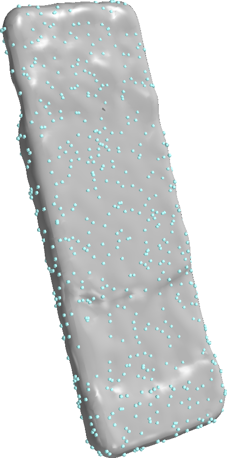
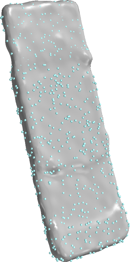
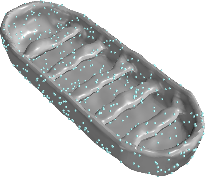
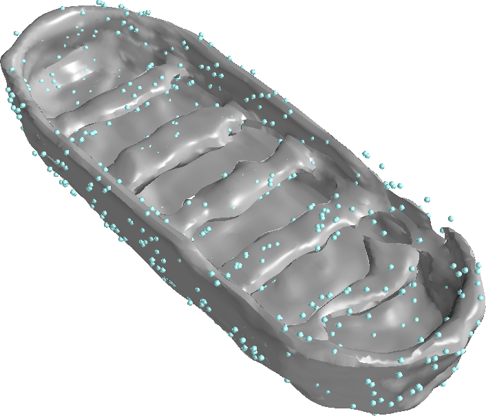
A.3 Additional Figures
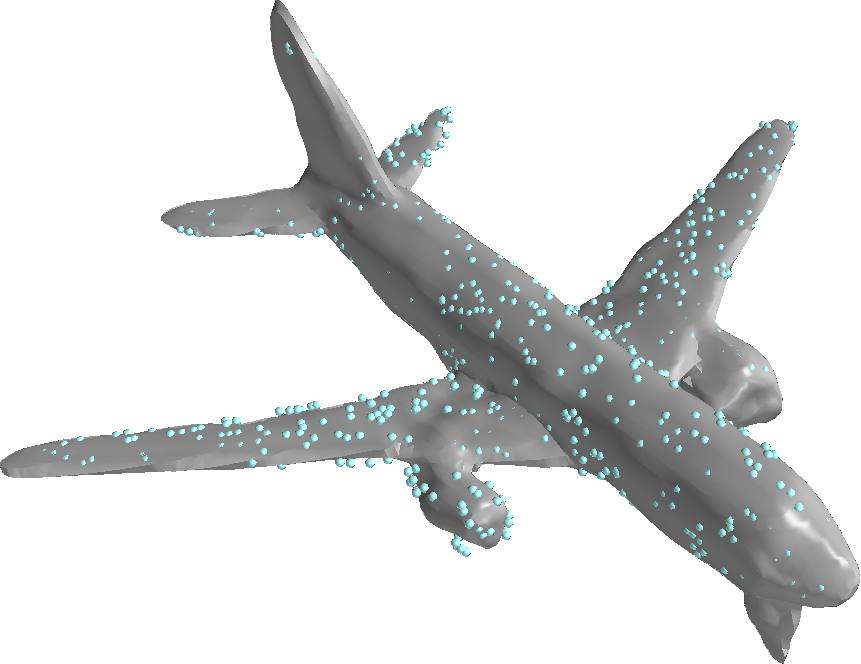
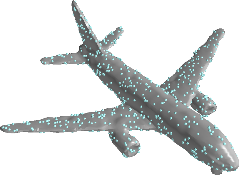
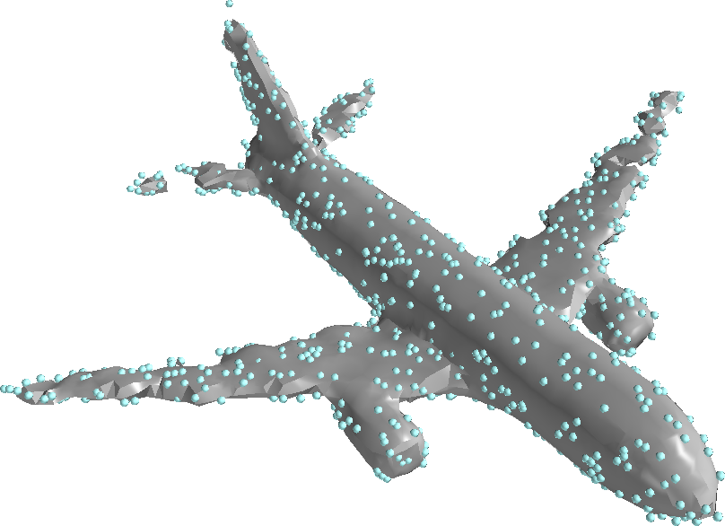
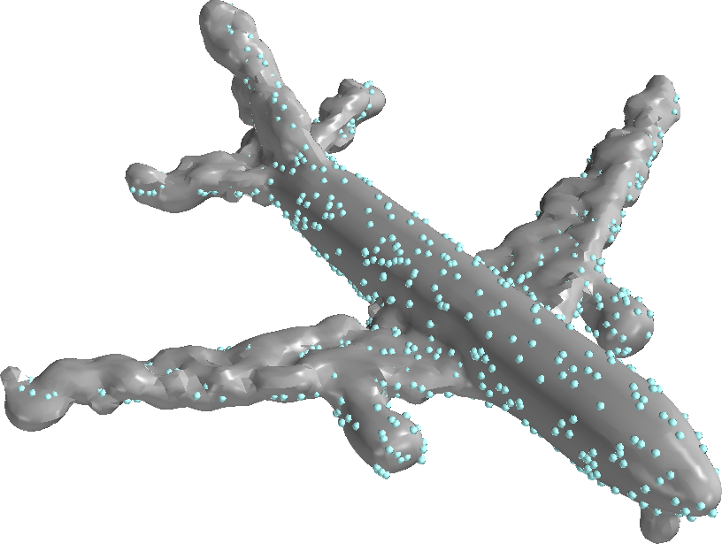
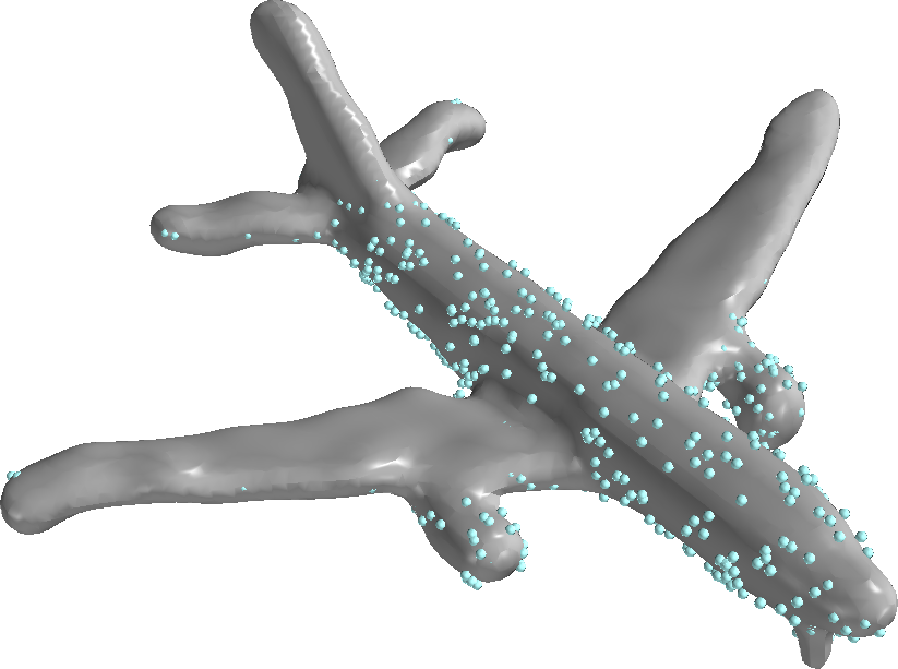
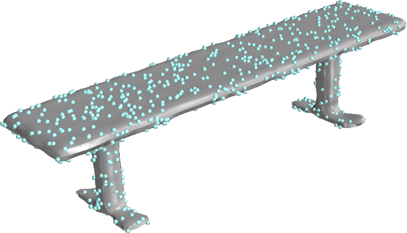
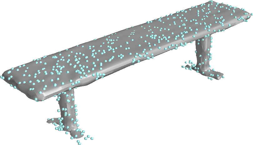
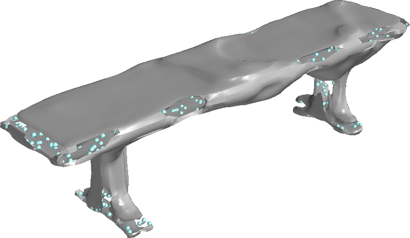
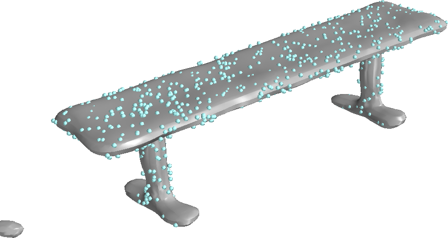
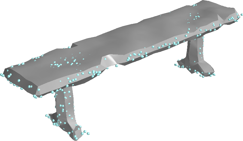
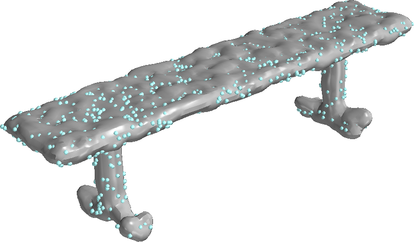
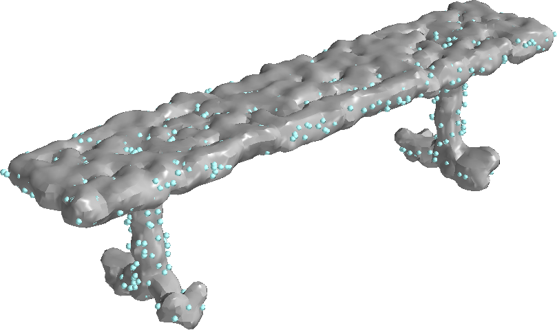
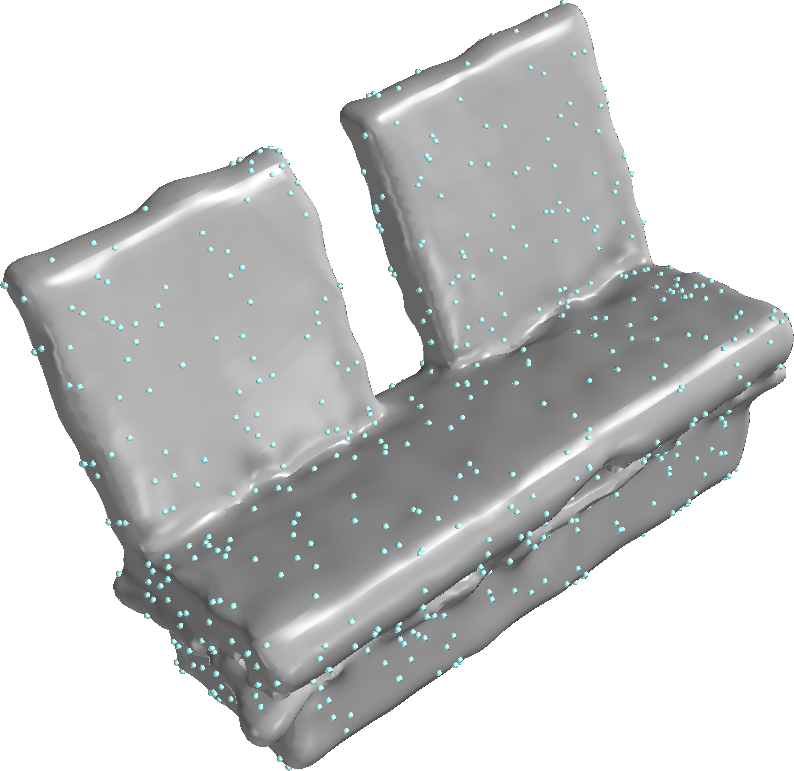
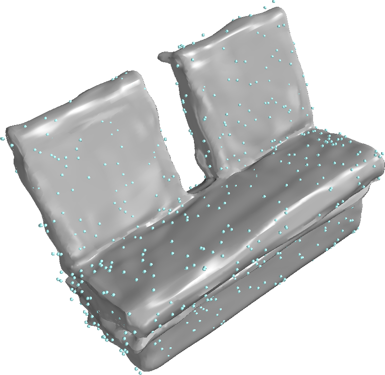
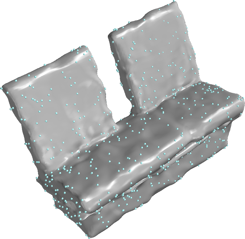
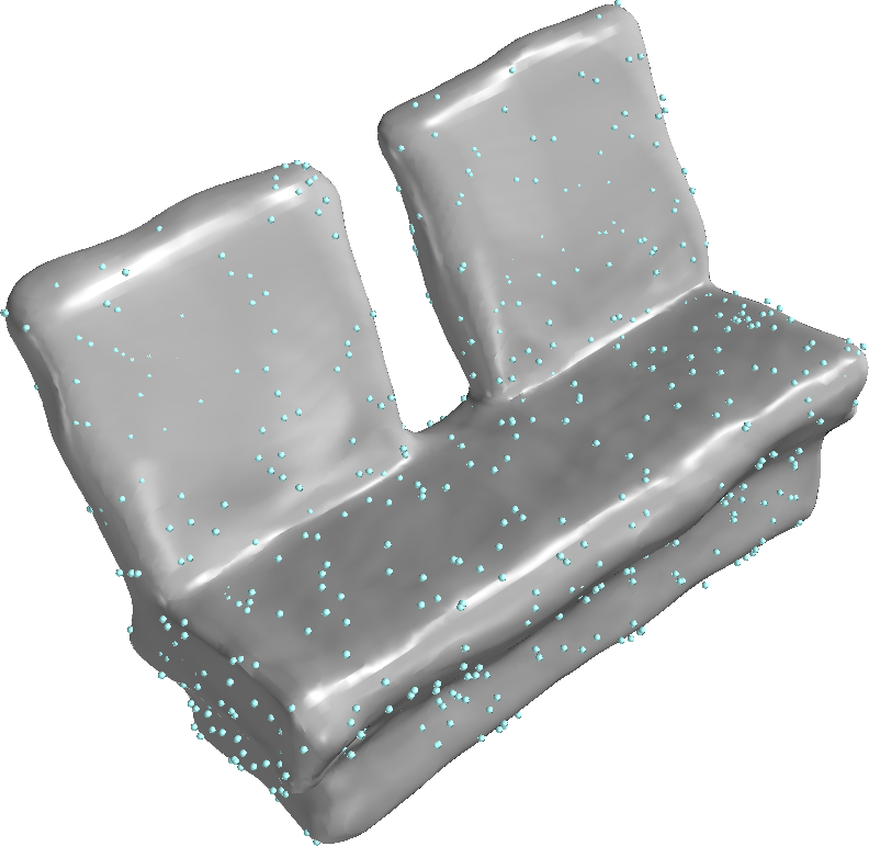
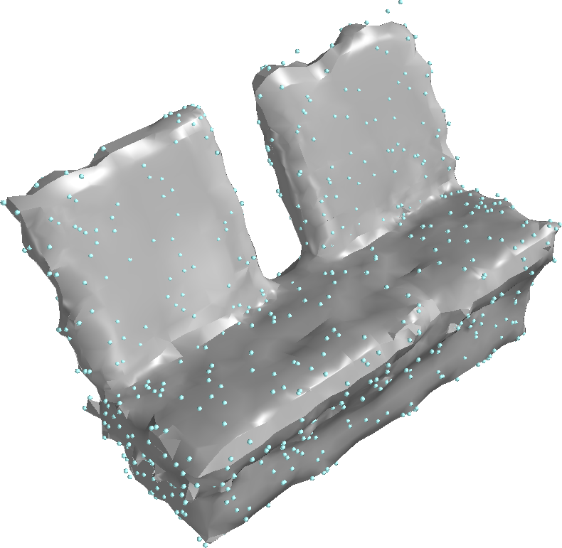
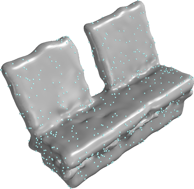
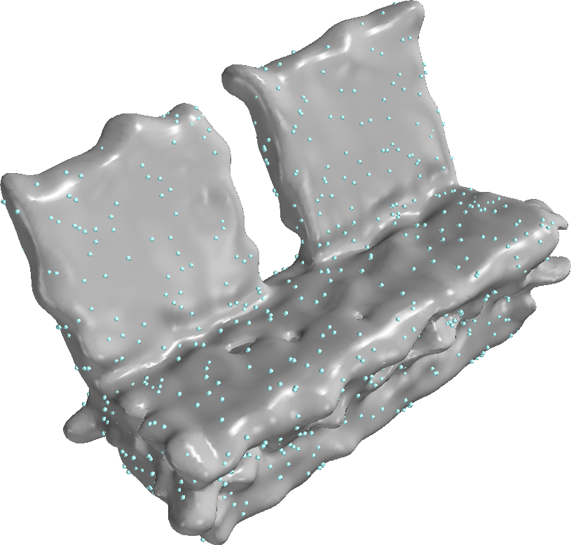
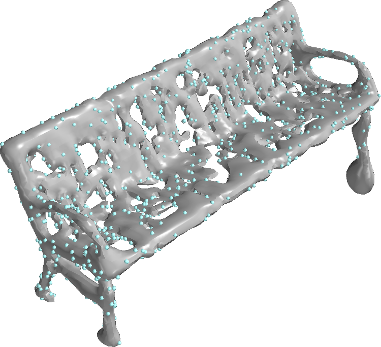
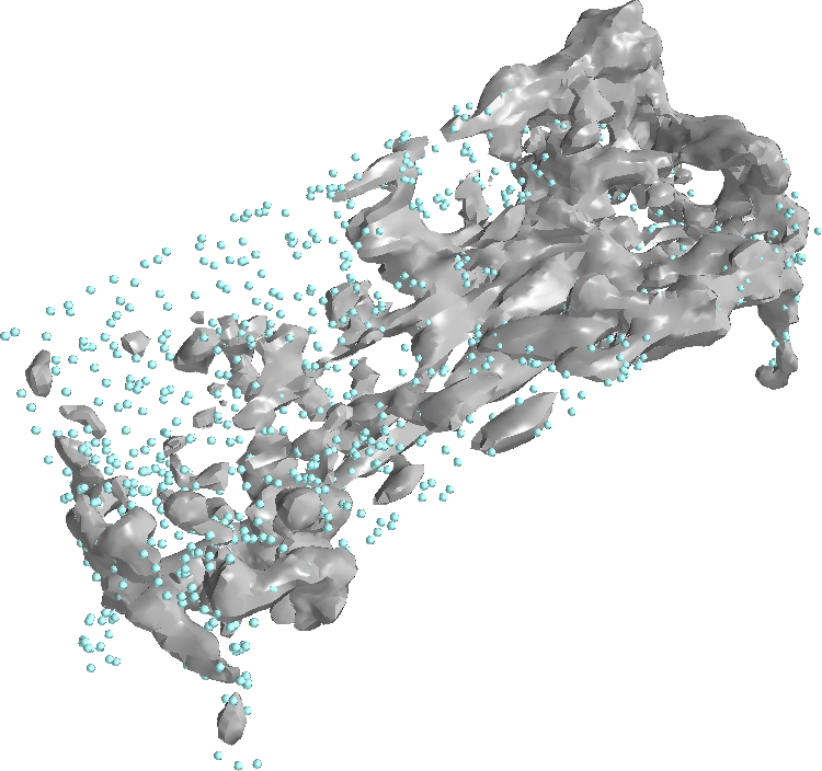
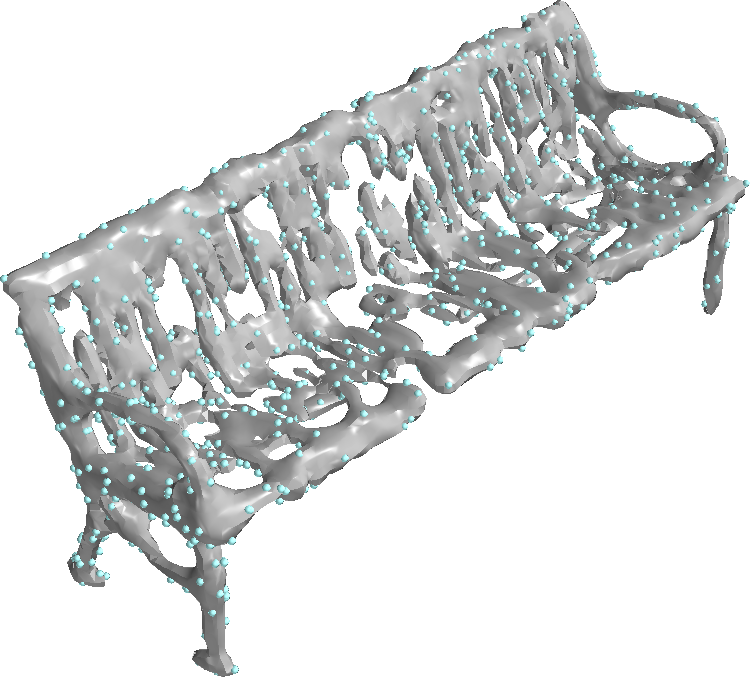
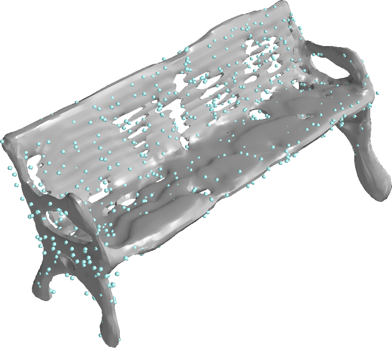
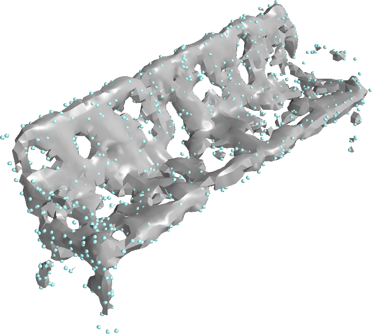
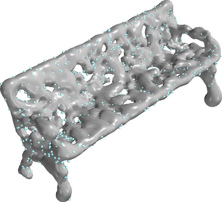
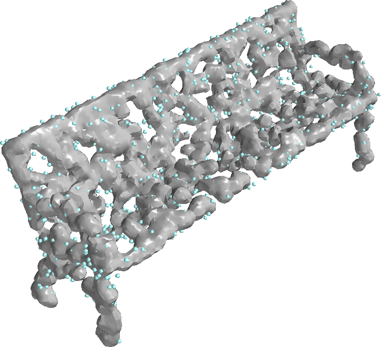
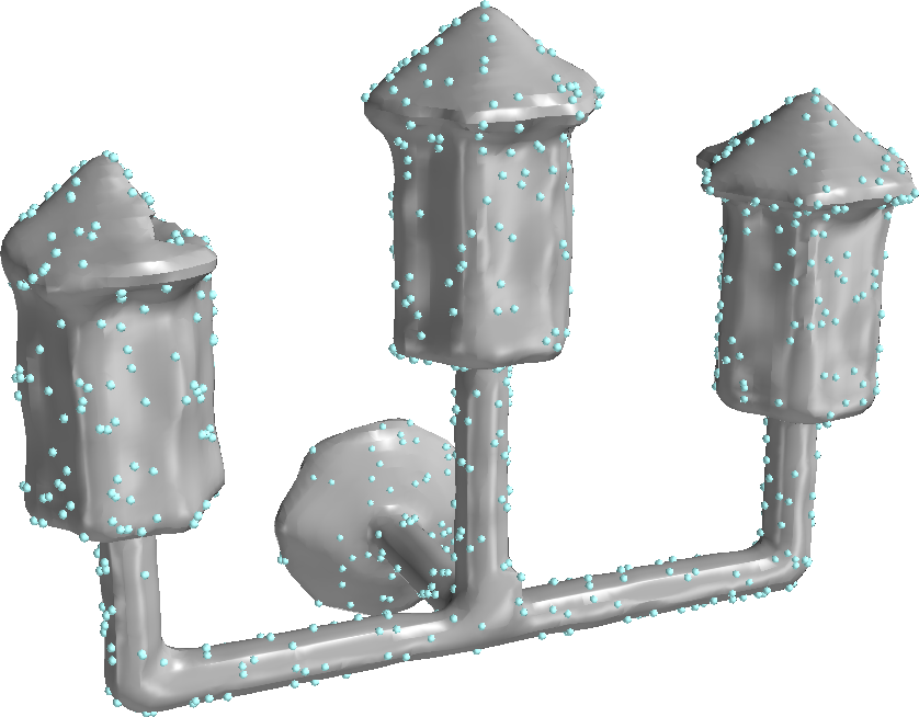
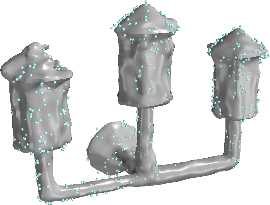
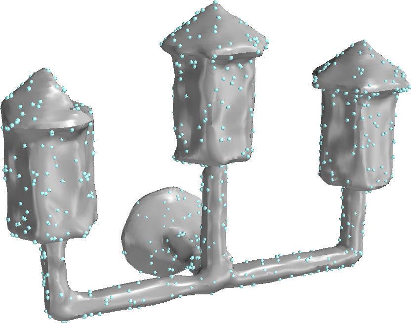
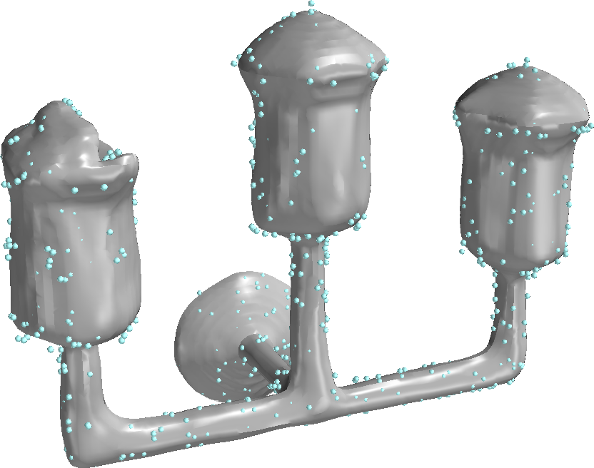
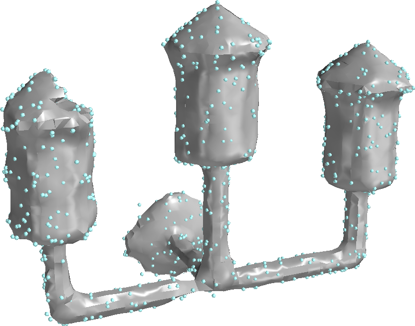
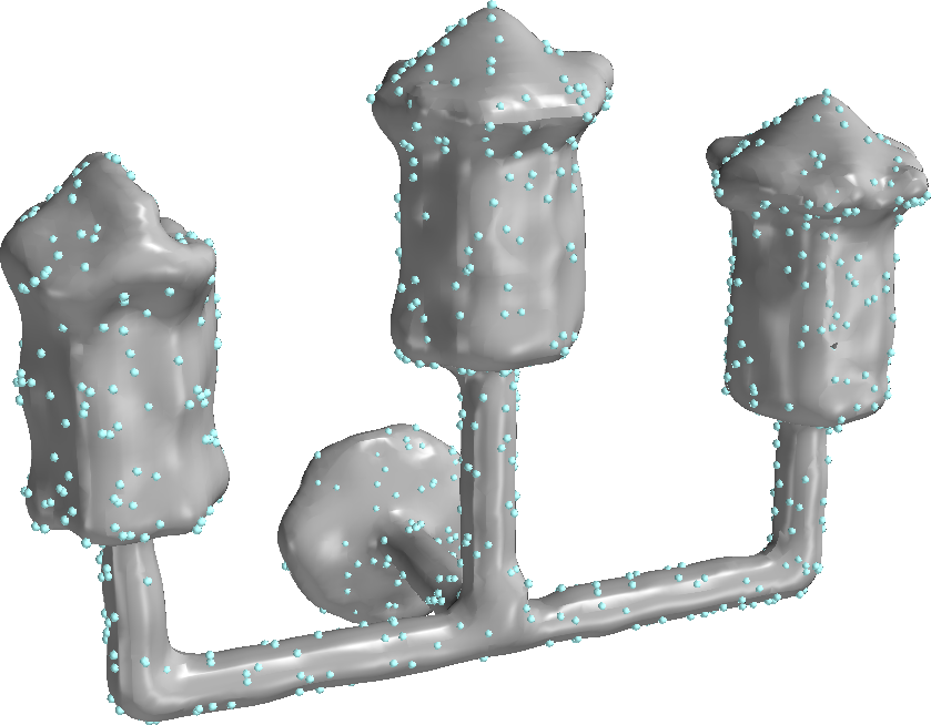
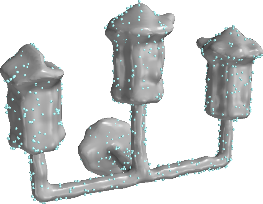
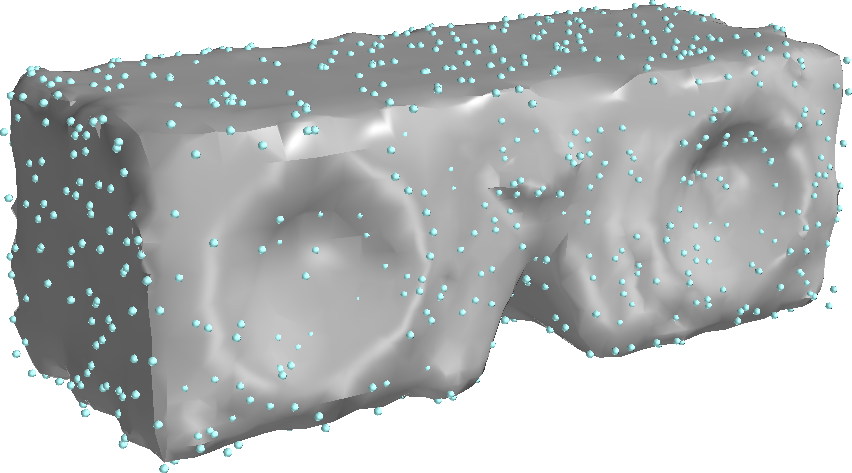
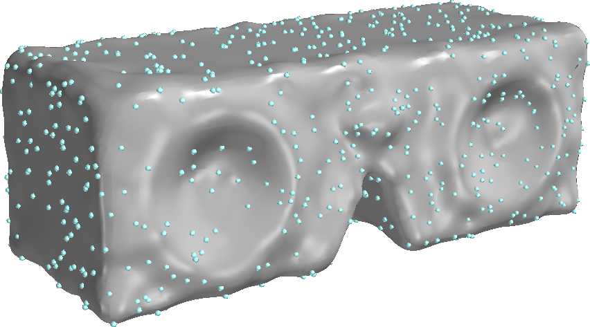
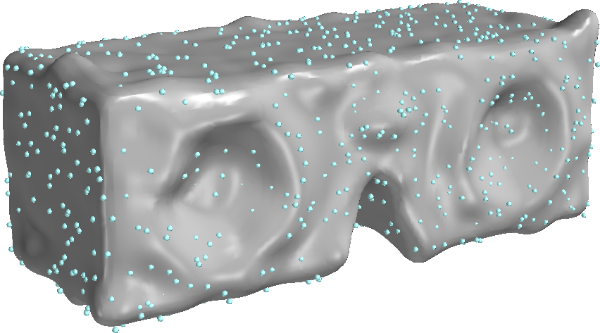
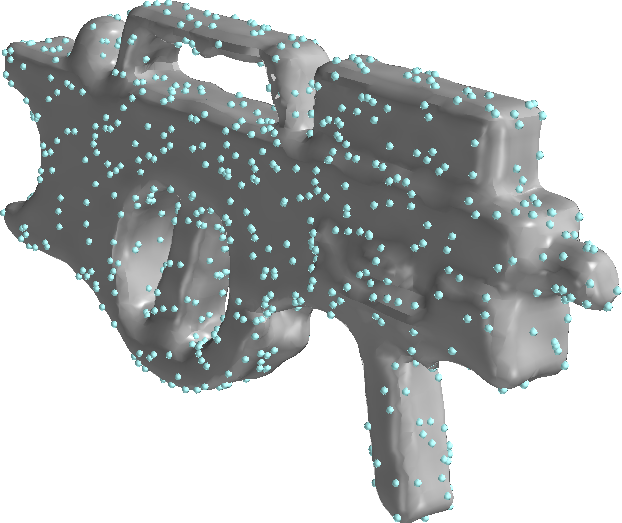
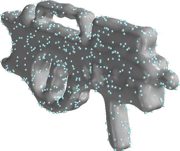
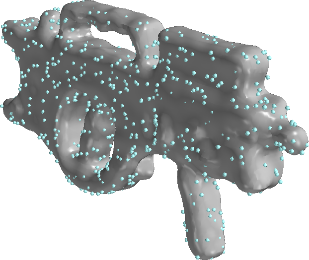
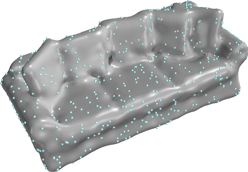
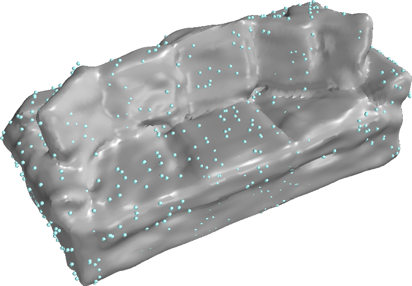
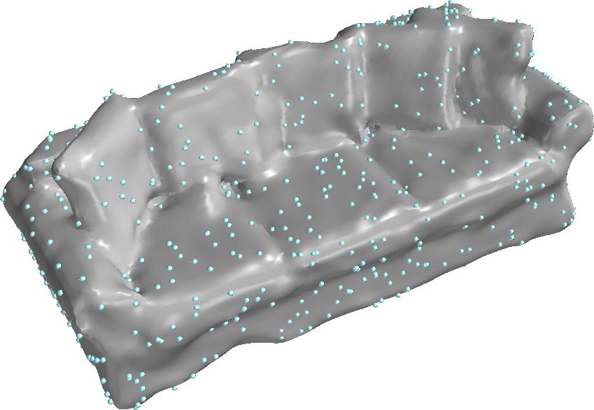
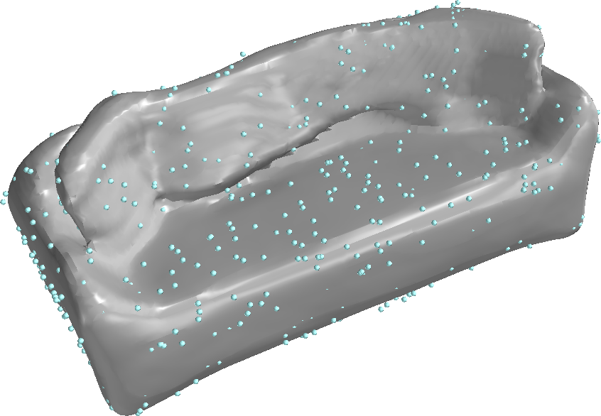
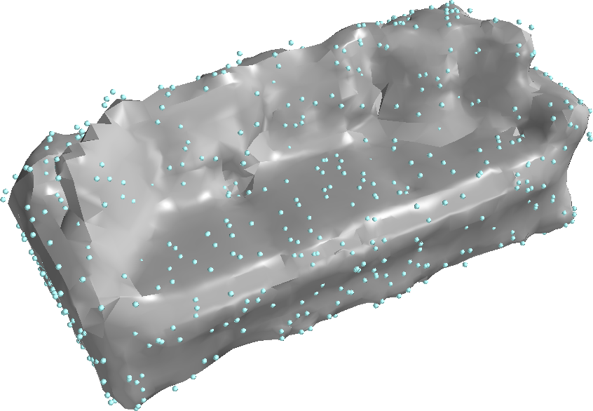
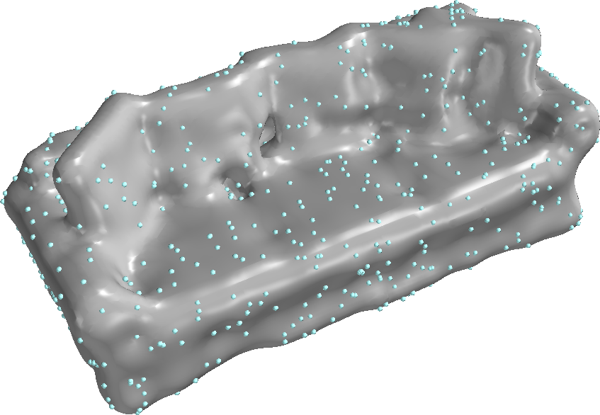
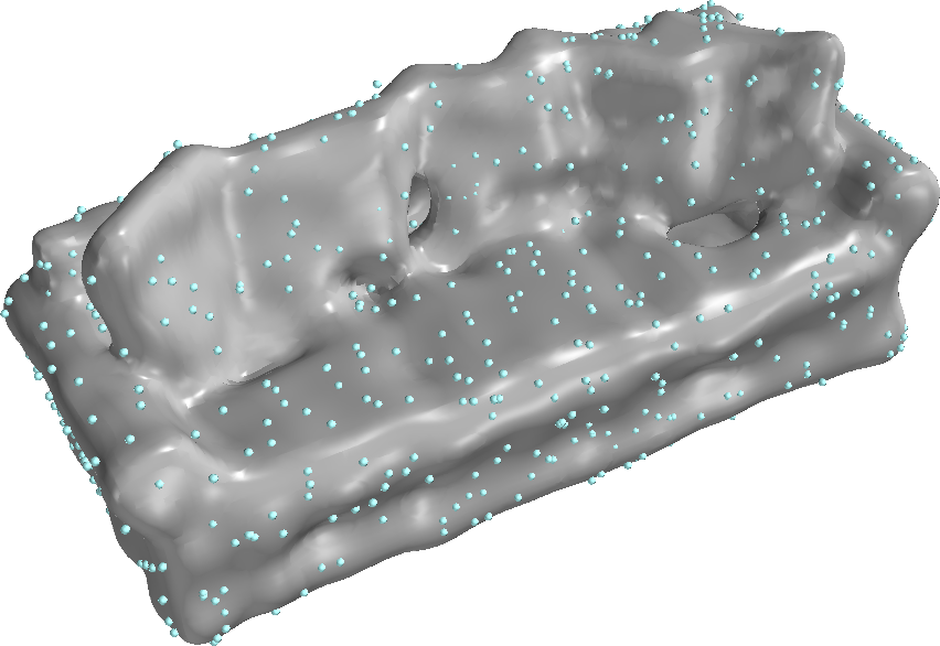
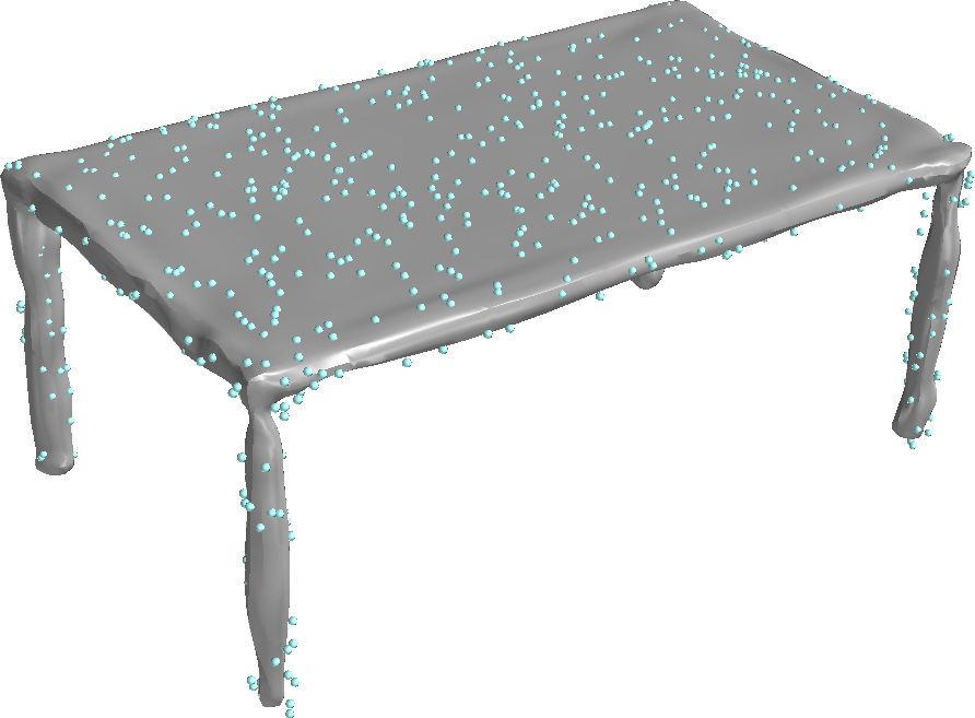
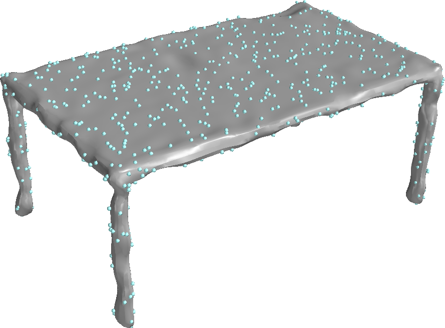
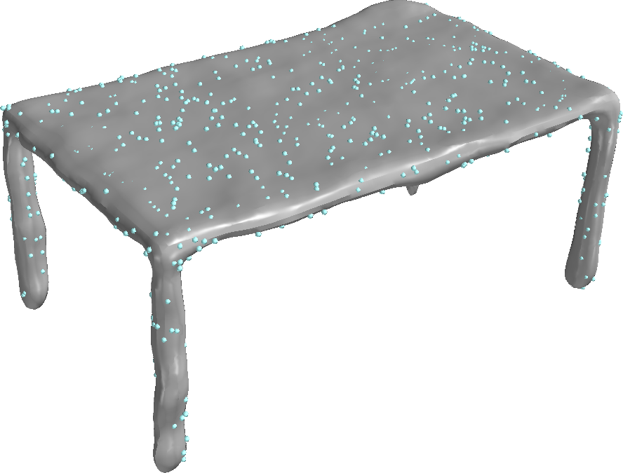
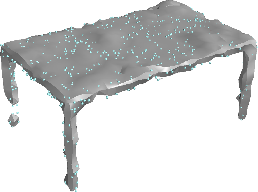
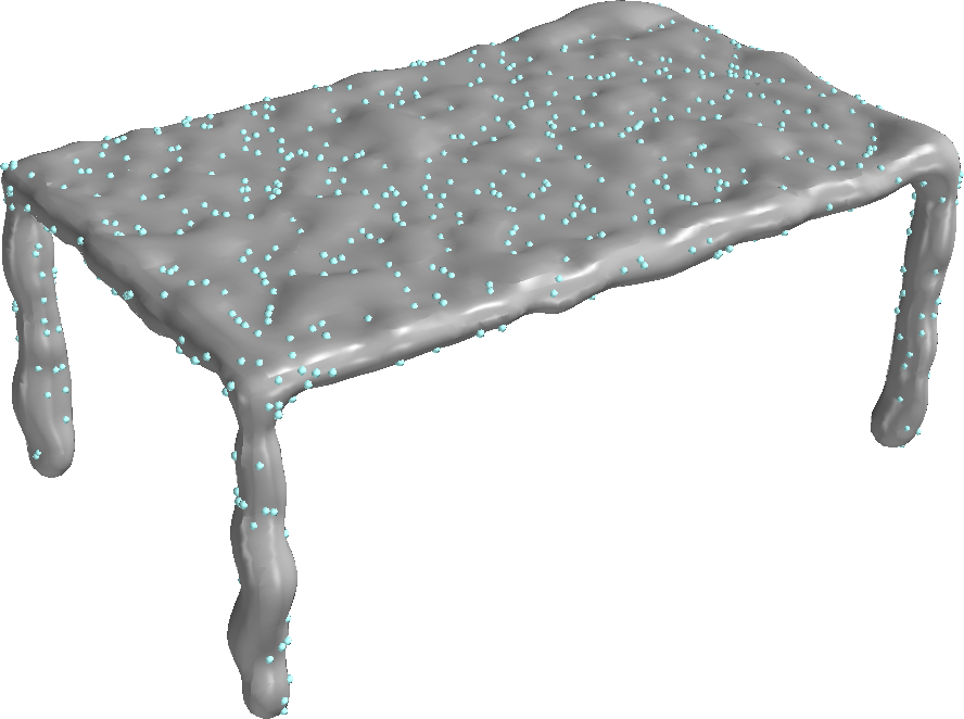
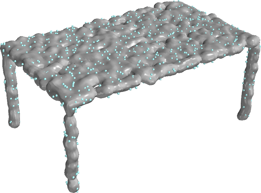
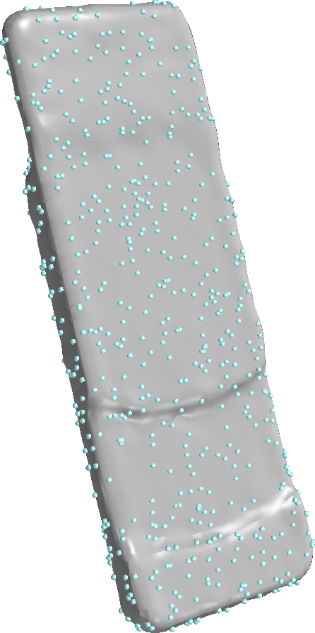
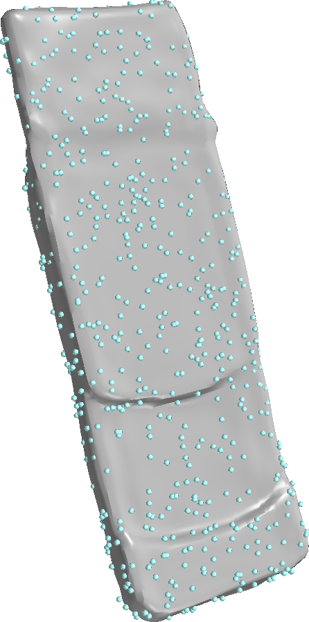
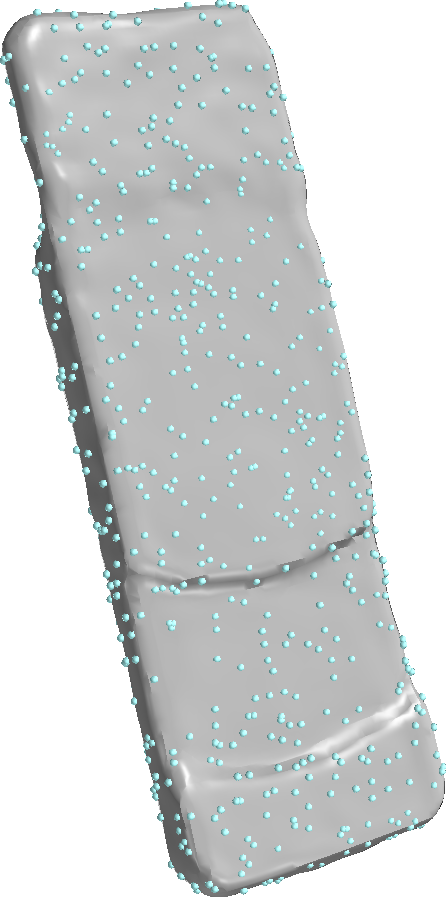
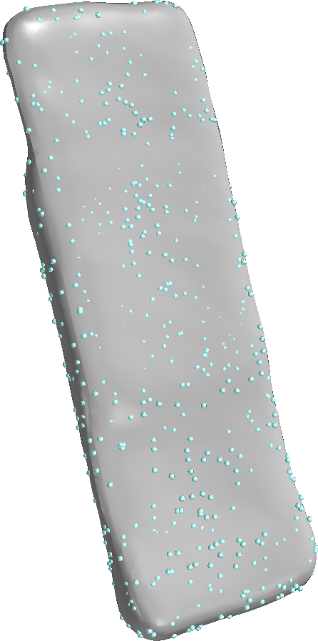
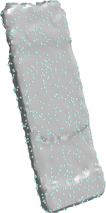
Figures 10 and 11 show at least one model reconstructed from each ShepeNet category using our method, Implicit Geometric Regularization (IGR) [24], SIREN [40], Fourier Feature Networks (FFN) [42], Screened Poisson Surface Reconstruction [31], Biharmonic RBF [9], and Support Vector Regression (SVR) [22]. Figure 12 shows the reconstructions of all the models from the Surface Reconstruction Benchmark [5] using our method, IGR [24], SIREN [40], and Fourier Feature Networks [42].
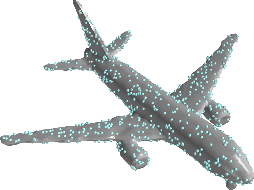



Ours
IGR
SIREN
Fourier Feats
Poisson
Biharmonic
SVR
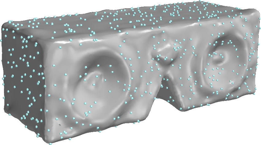
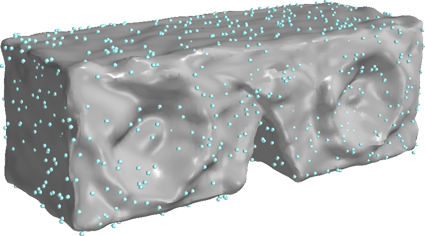
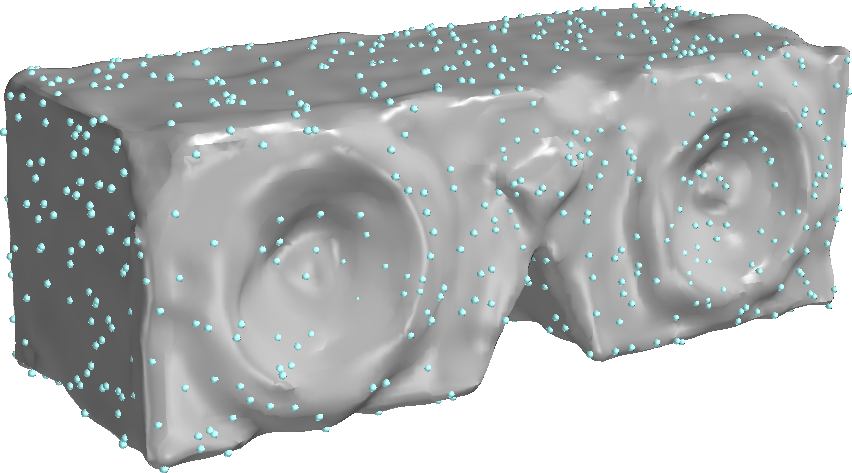
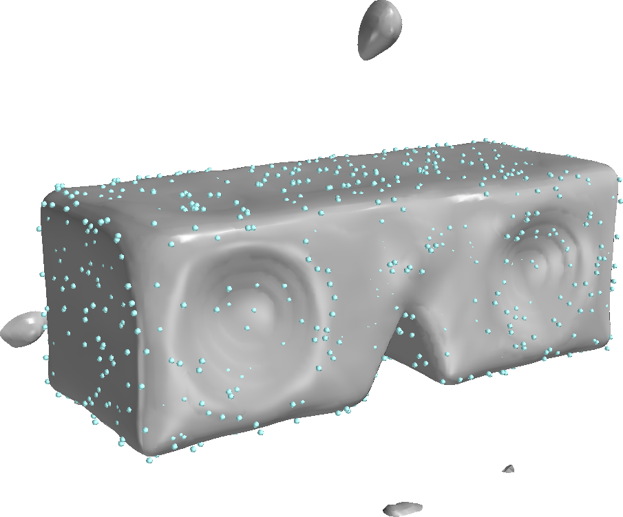
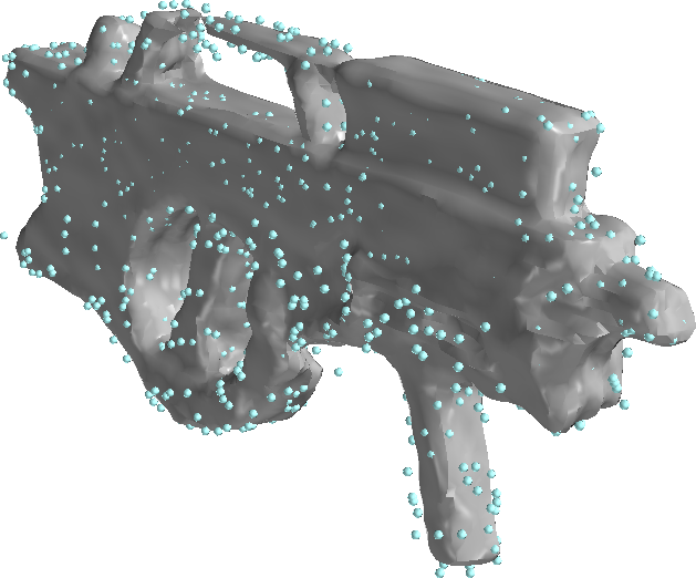
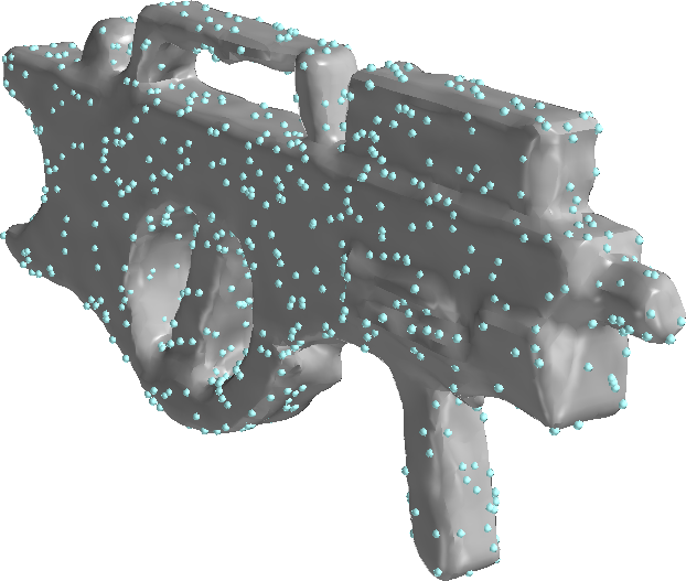
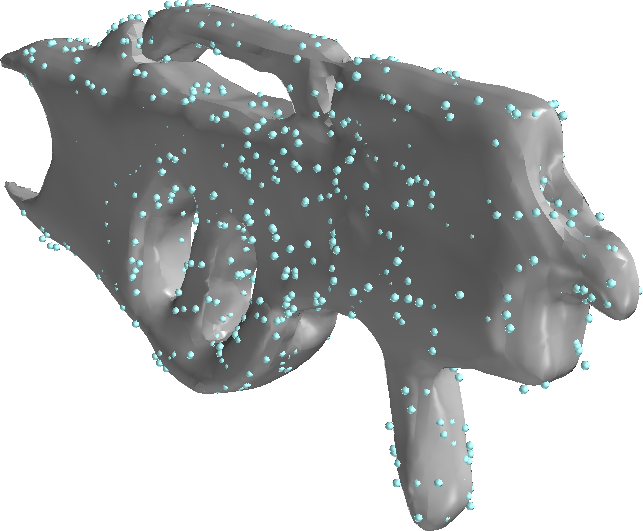
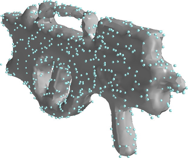

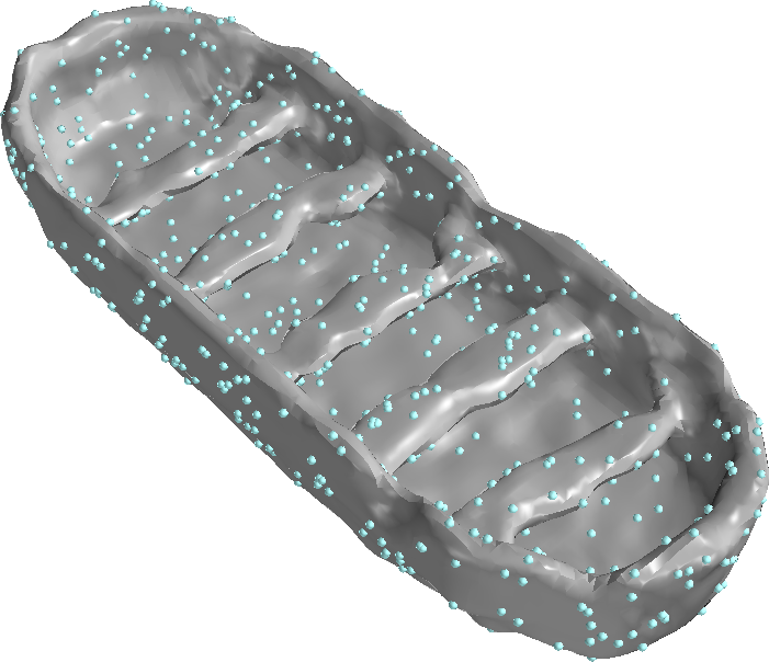
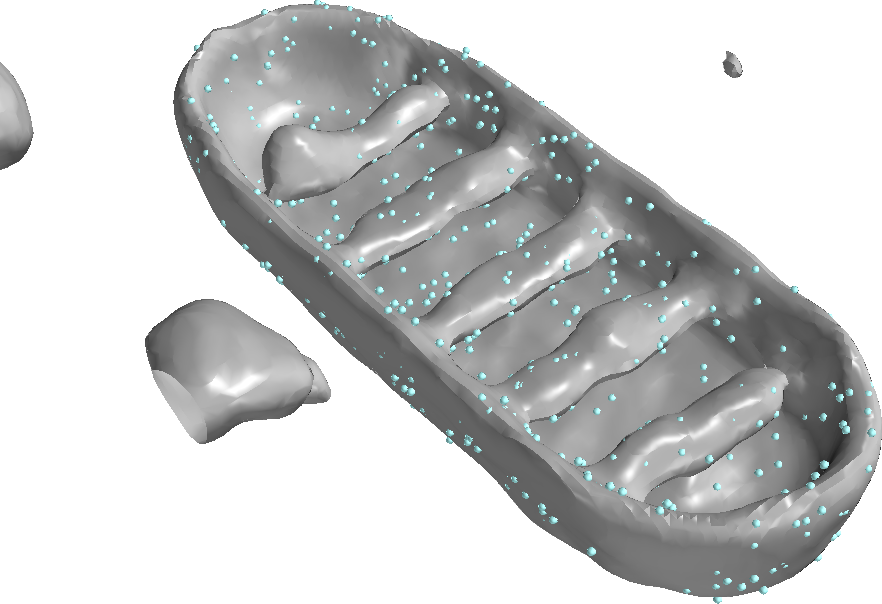
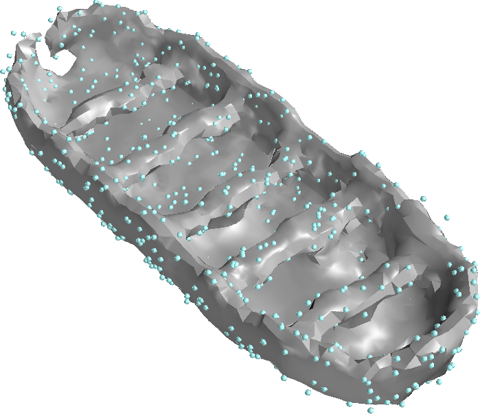
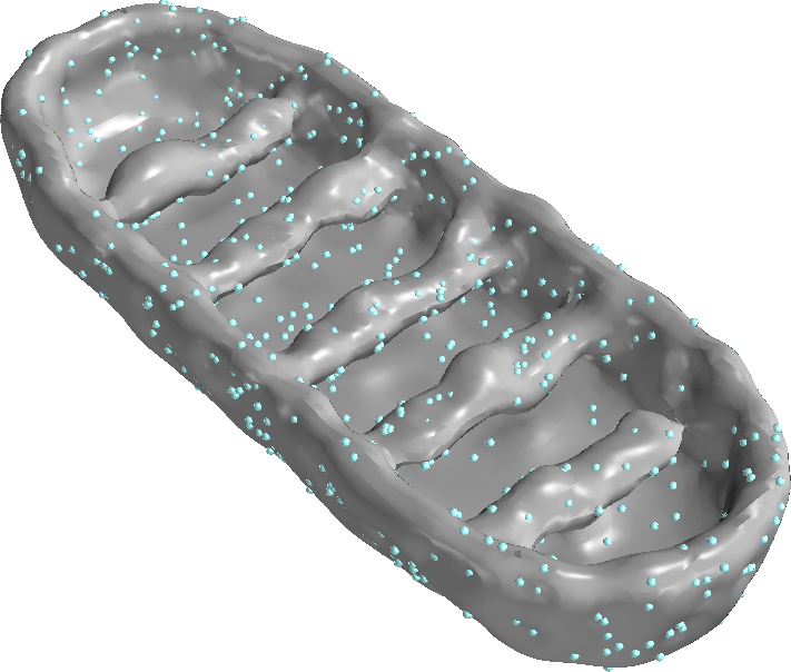
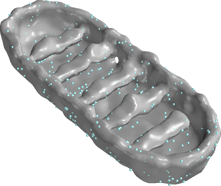
Ours
IGR
SIREN
Fourier Feats
Poisson
Biharmonic
SVR




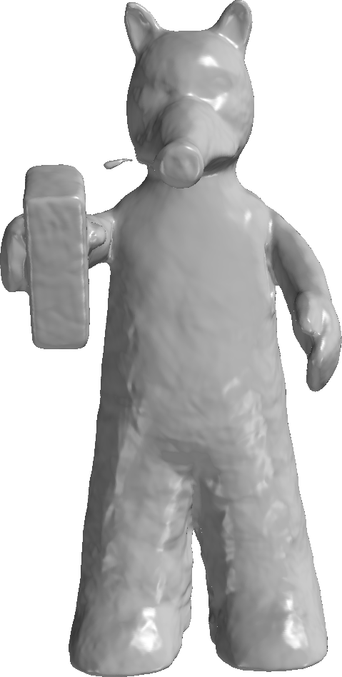
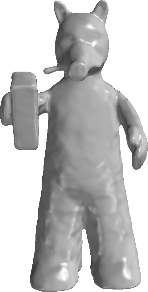
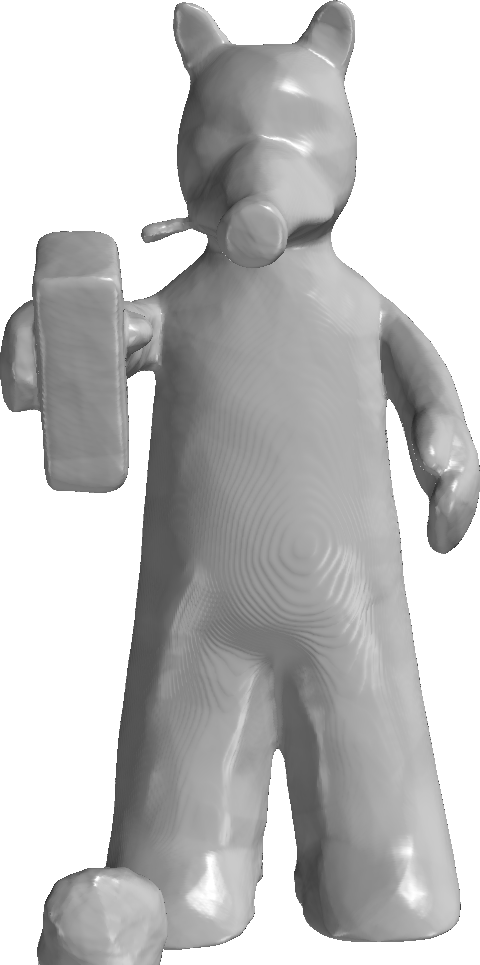
Ours
IGR
SIREN
Fourier Feats
A.4 Quantitative Results Per ShapeNet Class
Tables 4 show the per ShapeNet category IoU and Chamfer distance statistics for the benchmark described in Section 4.1.
| Intersection over Union (IoU) | |||||||||||||||||||||
| SIREN [40] | Fourier Feat. Nets [42] | Biharmonic RBF [9] | SVR [22] | Screened Poisson [31] | IGR [24] | Ours | |||||||||||||||
| Class | mean | median | std | mean | median | std | mean | median | std | mean | median | std | mean | median | std | mean | median | std | mean | median | std |
| airplane | 0.8045 | 0.9080 | 0.2696 | 0.6838 | 0.6926 | 0.0420 | 0.6690 | 0.7064 | 0.0809 | 0.6016 | 0.6257 | 0.0611 | 0.5954 | 0.6139 | 0.0581 | 0.7851 | 0.8193 | 0.0977 | 0.8165 | 0.8998 | 0.1551 |
| bench | 0.6109 | 0.7442 | 0.3258 | 0.6755 | 0.6583 | 0.1348 | 0.6237 | 0.6592 | 0.1682 | 0.6052 | 0.6282 | 0.1487 | 0.4728 | 0.4384 | 0.1213 | 0.5812 | 0.5923 | 0.2487 | 0.7872 | 0.8370 | 0.1236 |
| cabinet | 0.8706 | 0.9263 | 0.1621 | 0.8900 | 0.8984 | 0.0702 | 0.8913 | 0.9206 | 0.0926 | 0.7268 | 0.7142 | 0.0740 | 0.7301 | 0.7764 | 0.1095 | 0.8709 | 0.8857 | 0.0924 | 0.9274 | 0.9291 | 0.0422 |
| car | 0.8036 | 0.9241 | 0.2753 | 0.8173 | 0.8346 | 0.0847 | 0.8656 | 0.9020 | 0.1004 | 0.7903 | 0.8065 | 0.0773 | 0.6637 | 0.7192 | 0.1255 | 0.8026 | 0.8664 | 0.1300 | 0.8954 | 0.9288 | 0.0740 |
| chair | 0.8721 | 0.8807 | 0.0495 | 0.8250 | 0.8470 | 0.0618 | 0.8428 | 0.8667 | 0.0824 | 0.8127 | 0.8389 | 0.0839 | 0.5880 | 0.6046 | 0.1243 | 0.8049 | 0.8320 | 0.1022 | 0.8841 | 0.9034 | 0.0825 |
| display | 0.9014 | 0.9146 | 0.0440 | 0.8663 | 0.8755 | 0.0350 | 0.8470 | 0.8593 | 0.0738 | 0.8307 | 0.8407 | 0.0722 | 0.7027 | 0.7072 | 0.0800 | 0.8741 | 0.8917 | 0.0533 | 0.9309 | 0.9316 | 0.0251 |
| lamp | 0.8392 | 0.8995 | 0.2025 | 0.8192 | 0.8394 | 0.0773 | 0.8282 | 0.8706 | 0.1155 | 0.7728 | 0.7907 | 0.0963 | 0.5413 | 0.5786 | 0.1858 | 0.7865 | 0.8259 | 0.1318 | 0.9037 | 0.9178 | 0.0512 |
| loudspeaker | 0.8458 | 0.9618 | 0.2404 | 0.8993 | 0.9203 | 0.0709 | 0.9076 | 0.9621 | 0.1067 | 0.7098 | 0.6956 | 0.1193 | 0.7432 | 0.7848 | 0.1309 | 0.8867 | 0.9324 | 0.1017 | 0.9323 | 0.9627 | 0.0599 |
| rifle | 0.7329 | 0.9132 | 0.3662 | 0.7650 | 0.7693 | 0.0686 | 0.8350 | 0.8447 | 0.0845 | 0.7764 | 0.8013 | 0.0970 | 0.6803 | 0.6791 | 0.0532 | 0.8279 | 0.8267 | 0.0542 | 0.9299 | 0.9313 | 0.0215 |
| sofa | 0.9251 | 0.9411 | 0.0390 | 0.8805 | 0.8988 | 0.0554 | 0.9164 | 0.9377 | 0.0630 | 0.8694 | 0.8791 | 0.0740 | 0.7122 | 0.7326 | 0.0662 | 0.8891 | 0.9139 | 0.0708 | 0.9387 | 0.9473 | 0.0264 |
| table | 0.7280 | 0.8058 | 0.2089 | 0.7749 | 0.7786 | 0.0645 | 0.7096 | 0.7350 | 0.1150 | 0.6779 | 0.6596 | 0.1127 | 0.3720 | 0.3565 | 0.1334 | 0.6852 | 0.7260 | 0.2004 | 0.8414 | 0.8427 | 0.0534 |
| telephone | 0.9427 | 0.9514 | 0.0310 | 0.9111 | 0.9202 | 0.0483 | 0.9286 | 0.9433 | 0.0662 | 0.9195 | 0.9399 | 0.0638 | 0.7883 | 0.7990 | 0.0552 | 0.9148 | 0.9372 | 0.0639 | 0.9569 | 0.9625 | 0.0260 |
| watercraft | 0.8722 | 0.9279 | 0.1990 | 0.8180 | 0.8176 | 0.0545 | 0.8557 | 0.8756 | 0.0768 | 0.8197 | 0.8379 | 0.0742 | 0.6523 | 0.6793 | 0.0994 | 0.8146 | 0.8445 | 0.0931 | 0.9207 | 0.9231 | 0.0402 |
| All Classes: | 0.8268 | 0.9097 | 0.2329 | 0.8218 | 0.8396 | 0.0989 | 0.8247 | 0.8642 | 0.1350 | 0.7625 | 0.7819 | 0.1300 | 0.6340 | 0.6728 | 0.1577 | 0.8102 | 0.8480 | 0.1519 | 0.8973 | 0.9230 | 0.0871 |
| Chamfer Distance (CD) | |||||||||||||||||||||
| SIREN [40] | Fourier Feat. Nets [42] | Biharmonic RBF [9] | SVR [22] | Screened Poisson [31] | IGR [24] | Ours | |||||||||||||||
| Class | mean | median | std | mean | median | std | mean | median | std | mean | median | std | mean | median | std | mean | median | std | mean | median | std |
| airplane | 4.15e-5 | 3.87e-5 | 8.57e-6 | 1.04e-4 | 1.04e-4 | 1.02e-5 | 1.41e-4 | 1.31e-4 | 3.07e-5 | 1.61e-4 | 1.66e-4 | 1.01e-5 | 8.37e-5 | 8.76e-5 | 1.77e-5 | 3.04e-4 | 1.74e-4 | 3.47e-4 | 3.55e-5 | 3.44e-5 | 2.45e-6 |
| bench | 9.63e-5 | 8.12e-5 | 5.41e-5 | 9.45e-5 | 9.34e-5 | 2.10e-5 | 1.58e-4 | 1.73e-4 | 4.91e-5 | 1.34e-4 | 1.41e-4 | 3.05e-5 | 1.93e-4 | 1.93e-4 | 8.14e-5 | 4.48e-4 | 2.58e-4 | 4.33e-4 | 5.66e-5 | 4.82e-5 | 2.09e-5 |
| cabinet | 1.51e-4 | 6.69e-5 | 1.77e-4 | 1.01e-4 | 8.89e-5 | 3.86e-5 | 1.29e-4 | 1.19e-4 | 7.81e-5 | 1.34e-4 | 1.30e-4 | 8.27e-5 | 3.62e-4 | 2.91e-4 | 1.96e-4 | 1.56e-4 | 9.39e-5 | 1.23e-4 | 6.98e-5 | 4.69e-5 | 4.34e-5 |
| car | 1.39e-4 | 9.07e-5 | 1.03e-4 | 1.17e-4 | 1.10e-4 | 2.96e-5 | 1.17e-4 | 1.00e-4 | 5.23e-5 | 1.23e-4 | 1.18e-4 | 3.90e-5 | 2.27e-4 | 2.22e-4 | 8.04e-5 | 2.60e-4 | 2.82e-4 | 9.80e-5 | 8.21e-5 | 7.18e-5 | 3.60e-5 |
| chair | 1.05e-4 | 6.34e-5 | 1.18e-4 | 1.00e-4 | 8.85e-5 | 4.23e-5 | 1.10e-4 | 9.60e-5 | 6.11e-5 | 1.11e-4 | 1.01e-4 | 5.66e-5 | 2.82e-4 | 2.13e-4 | 1.84e-4 | 9.25e-4 | 9.88e-5 | 3.11e-3 | 5.62e-5 | 4.21e-5 | 4.32e-5 |
| display | 6.98e-5 | 5.68e-5 | 3.86e-5 | 7.60e-5 | 7.32e-5 | 2.36e-5 | 9.85e-5 | 9.06e-5 | 3.42e-5 | 9.86e-5 | 1.01e-4 | 3.35e-5 | 2.45e-4 | 2.13e-4 | 1.11e-4 | 9.99e-5 | 7.49e-5 | 8.44e-5 | 4.36e-5 | 3.99e-5 | 1.28e-5 |
| lamp | 6.26e-5 | 5.07e-5 | 3.35e-5 | 7.79e-5 | 7.97e-5 | 1.33e-5 | 9.26e-5 | 8.05e-5 | 4.81e-5 | 1.10e-4 | 1.02e-4 | 4.26e-5 | 1.61e-4 | 1.35e-4 | 1.02e-4 | 1.72e-3 | 1.28e-4 | 6.24e-3 | 4.19e-5 | 3.91e-5 | 1.00e-5 |
| loudspeaker | 2.77e-4 | 6.88e-5 | 5.54e-4 | 1.07e-4 | 9.22e-5 | 4.66e-5 | 1.36e-4 | 7.94e-5 | 1.16e-4 | 1.36e-4 | 9.91e-5 | 1.02e-4 | 4.29e-4 | 3.54e-4 | 2.68e-4 | 3.77e-3 | 1.15e-4 | 1.49e-2 | 8.41e-5 | 4.54e-5 | 7.54e-5 |
| rifle | 3.62e-5 | 3.50e-5 | 4.03e-6 | 7.17e-5 | 7.05e-5 | 1.43e-5 | 5.04e-5 | 5.00e-5 | 9.36e-6 | 7.20e-5 | 7.12e-5 | 1.46e-5 | 4.46e-5 | 3.11e-5 | 2.76e-5 | 9.62e-5 | 5.29e-5 | 1.25e-4 | 3.26e-5 | 3.15e-5 | 2.79e-6 |
| sofa | 7.88e-5 | 6.99e-5 | 3.90e-5 | 9.77e-5 | 9.59e-5 | 2.48e-5 | 8.42e-5 | 7.72e-5 | 3.17e-5 | 9.46e-5 | 9.02e-5 | 3.39e-5 | 2.72e-4 | 2.46e-4 | 1.02e-4 | 2.86e-4 | 1.02e-4 | 5.30e-4 | 5.11e-5 | 4.80e-5 | 1.24e-5 |
| table | 1.92e-4 | 8.32e-5 | 2.32e-4 | 1.02e-4 | 9.35e-5 | 3.62e-5 | 1.96e-4 | 1.91e-4 | 8.62e-5 | 1.66e-4 | 1.60e-4 | 6.73e-5 | 3.50e-4 | 2.53e-4 | 2.14e-4 | 3.40e-4 | 1.95e-4 | 3.33e-4 | 6.60e-5 | 4.88e-5 | 4.17e-5 |
| telephone | 3.88e-5 | 3.58e-5 | 9.64e-6 | 4.91e-5 | 4.63e-5 | 1.28e-5 | 4.90e-5 | 4.04e-5 | 2.93e-5 | 4.77e-5 | 4.06e-5 | 2.19e-5 | 1.28e-4 | 1.17e-4 | 3.36e-5 | 1.03e-4 | 4.43e-5 | 1.54e-4 | 3.34e-5 | 3.19e-5 | 3.60e-6 |
| watercraft | 5.57e-5 | 4.21e-5 | 2.95e-5 | 9.05e-5 | 8.46e-5 | 2.18e-5 | 7.81e-5 | 6.73e-5 | 3.89e-5 | 9.47e-5 | 8.56e-5 | 3.07e-5 | 1.07e-4 | 8.82e-5 | 6.12e-5 | 1.47e-4 | 1.12e-4 | 1.23e-4 | 4.41e-5 | 3.84e-5 | 1.42e-5 |
| All Classes: | 1.03e-4 | 5.28e-5 | 1.93e-4 | 9.12e-5 | 8.65e-5 | 3.36e-5 | 1.11e-4 | 8.97e-5 | 7.06e-5 | 1.14e-4 | 1.04e-4 | 5.99e-5 | 2.22e-4 | 1.70e-4 | 1.76e-4 | 6.66e-4 | 1.07e-4 | 4.69e-3 | 5.36e-5 | 4.06e-5 | 3.64e-5 |
A.5 Per Model Performance Numbers
Table 5 shows the runtime and GPU usage required to reconstruct each model in the Surface Reconstruction Benchmark. For our model, we used 15k Nyström samples and a regularization of 1e-11. We do not report CPU memory usage since it is hard to profile exactly, however we observed that none of the methods used more than 4GiB of CPU memory. All timings were done on a machine with a single NVIDIA-V100 GPU with 16GiB of VRAM, 32GiB of CPU RAM, and and an 8 core Intel Xeon processor.
| Method | Runtime (seconds) | GPU Memory | |
|---|---|---|---|
| Anchor | IGR [24] | 1726.84 | 5093 |
| SIREN [40] | 684.66 | 1855 | |
| FFN [42] | 385.90 | 4266 | |
| Poisson [31] | 2.35 | N.A. | |
| Ours | 13.22 | 5528 | |
| Daratech | IGR [24] | 1239.43 | 5093 |
| SIREN [40] | 500.42 | 1855 | |
| FFN [42] | 281.61 | 4266 | |
| Poisson [31] | 1.83 | N.A. | |
| Ours | 10.75 | 5528 | |
| DC | IGR [24] | 1443.65 | 5093 |
| SIREN [40] | 576.83 | 1545 | |
| FFN [42] | 325.10 | 3565 | |
| Poisson [31] | 1.41 | N.A. | |
| Ours | 12.31 | 5510 | |
| Gargoyle | IGR [24] | 1646.44 | 5093 |
| SIREN [40] | 766.27 | 2076 | |
| FFN [42] | 432.59 | 4778 | |
| Poisson [31] | 1.44 | N.A. | |
| Ours | 12.87 | 5145 | |
| Lord Quas | IGR [24] | 1013.33 | 5093 |
| SIREN [40] | 466.82 | 1237 | |
| FFN [42] | 263.34 | 2870 | |
| Poisson [31] | 1.21 | N.A. | |
| Ours | 10.41 | 5281 |
A.6 Empirical versus Analytical Kernel
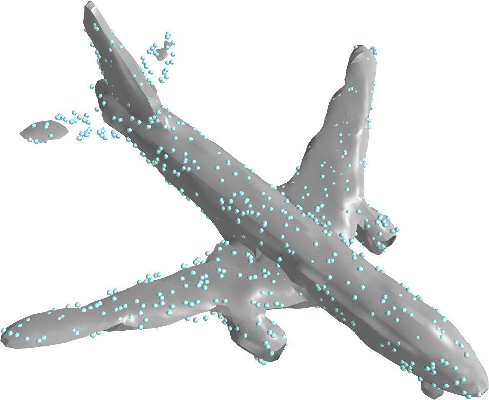
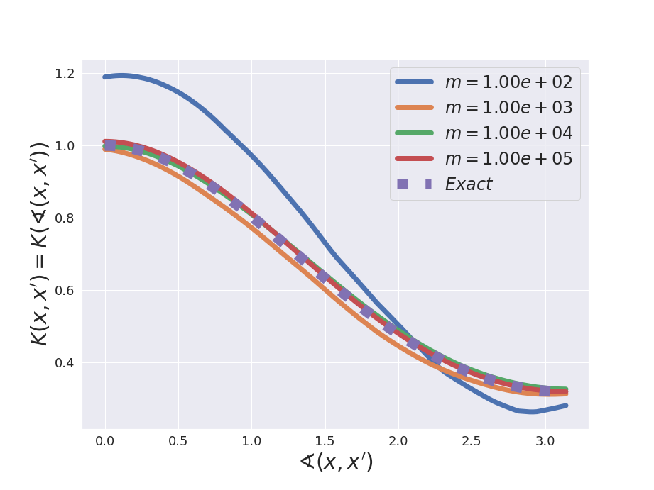
Figure 14 compares results using the empirical kernel with neurons and using the analytical kernel. Figure 13 shows the convergence of the empirical Kernel to the analytic one as the number of neurons grows.
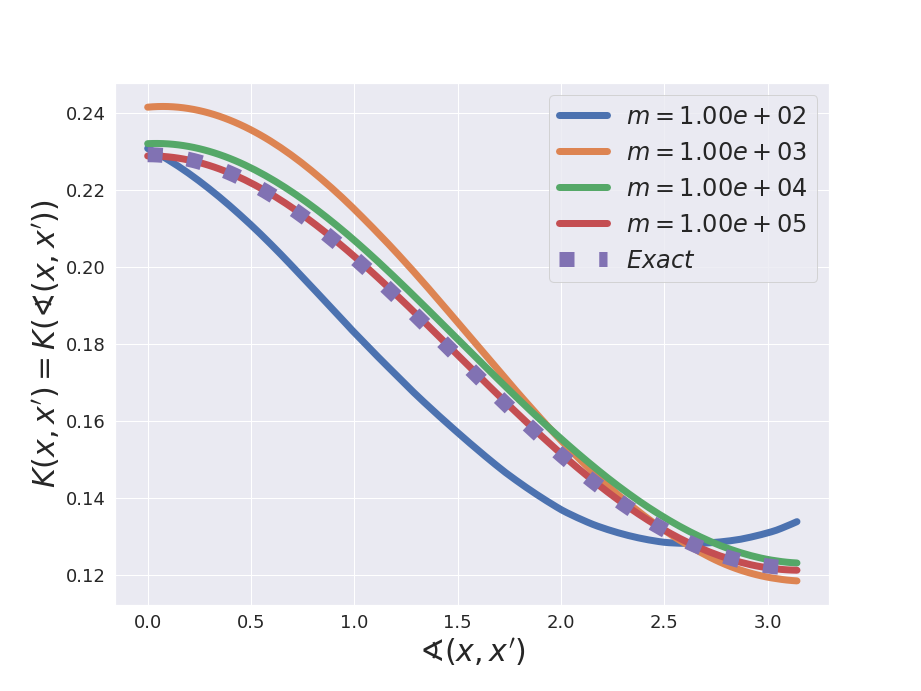
Gaussian Kernel
Uniform Kernel
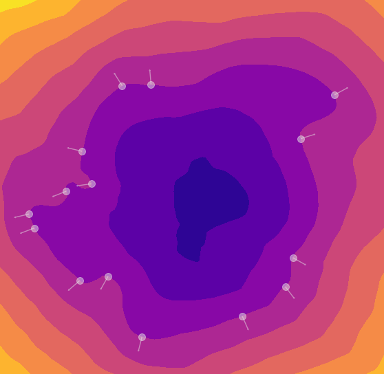
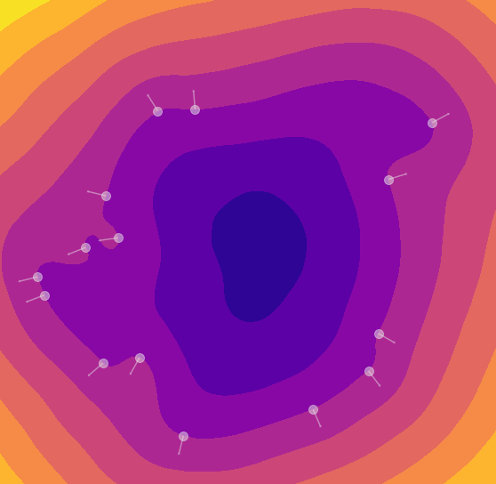
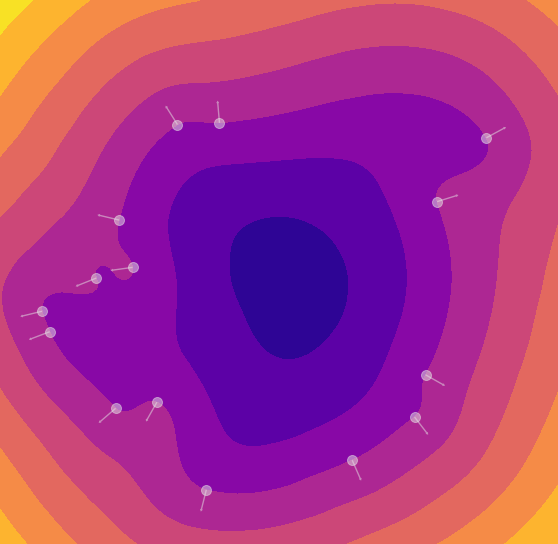

= 1k
= 10k
= 50k
Analytical
A.7 Quantitative Comparison between Gaussian and Uniform Kernels
Table 6 shows a quantitative comparison between Neural Splines using the Gaussian initialization (9) and the Uniform initialization (8) on the benchmark described in Section (4.1). The results in both cases are very close to each other in both Chamfer distance and in IoU.
| Intersection over Union (IoU) | ||||||
| Neural Spline (Uniform) | Neural Spline (Gaussian) | |||||
| Class | mean | median | std | mean | median | std |
| car | 0.9082 | 0.9399 | 0.0747 | 0.9084 | 0.9392 | 0.0743 |
| chair | 0.9056 | 0.9369 | 0.1062 | 0.9131 | 0.9357 | 0.0852 |
| airplane | 0.7773 | 0.8796 | 0.1961 | 0.8388 | 0.9159 | 0.1531 |
| display | 0.9533 | 0.9549 | 0.0188 | 0.9523 | 0.9535 | 0.0193 |
| table | 0.8968 | 0.9011 | 0.0500 | 0.8952 | 0.8980 | 0.0508 |
| rifle | 0.9489 | 0.9491 | 0.0169 | 0.9488 | 0.9498 | 0.0185 |
| cabinet | 0.9478 | 0.9467 | 0.0377 | 0.9477 | 0.9475 | 0.0377 |
| loudspeaker | 0.9507 | 0.9768 | 0.0518 | 0.9500 | 0.9768 | 0.0531 |
| telephone | 0.9746 | 0.9772 | 0.0202 | 0.9741 | 0.9774 | 0.0209 |
| bench | 0.8160 | 0.8900 | 0.1365 | 0.8195 | 0.8902 | 0.1296 |
| sofa | 0.9565 | 0.9644 | 0.0267 | 0.9584 | 0.9643 | 0.0221 |
| watercraft | 0.9340 | 0.9380 | 0.0462 | 0.9360 | 0.9386 | 0.0404 |
| lamp | 0.9467 | 0.9470 | 0.0306 | 0.9457 | 0.9459 | 0.0319 |
| All Classes: | 0.9167 | 0.9438 | 0.0985 | 0.9221 | 0.9441 | 0.0834 |
| Chamfer Distance (CD) | ||||||
| Neural Spline (Uniform) | Neural Spline (Gaussian) | |||||
| Class | mean | median | std | mean | median | std |
| car | 8.21e-05 | 7.23e-05 | 3.59e-05 | 8.21e-05 | 7.18e-05 | 3.60e-05 |
| chair | 5.52e-05 | 4.20e-05 | 4.01e-05 | 5.62e-05 | 4.21e-05 | 4.32e-05 |
| airplane | 3.55e-05 | 3.45e-05 | 2.45e-06 | 3.55e-05 | 3.44e-05 | 2.45e-06 |
| display | 4.31e-05 | 3.95e-05 | 1.24e-05 | 4.36e-05 | 3.99e-05 | 1.28e-05 |
| table | 6.44e-05 | 4.78e-05 | 4.01e-05 | 6.60e-05 | 4.88e-05 | 4.17e-05 |
| rifle | 3.27e-05 | 3.16e-05 | 2.81e-06 | 3.26e-05 | 3.15e-05 | 2.79e-06 |
| cabinet | 6.93e-05 | 4.67e-05 | 4.30e-05 | 6.98e-05 | 4.69e-05 | 4.34e-05 |
| loudspeaker | 8.27e-05 | 4.58e-05 | 7.24e-05 | 8.41e-05 | 4.54e-05 | 7.54e-05 |
| telephone | 3.33e-05 | 3.18e-05 | 3.42e-06 | 3.34e-05 | 3.19e-05 | 3.60e-06 |
| bench | 5.62e-05 | 4.74e-05 | 2.05e-05 | 5.66e-05 | 4.82e-05 | 2.09e-05 |
| sofa | 5.08e-05 | 4.81e-05 | 1.22e-05 | 5.11e-05 | 4.80e-05 | 1.24e-05 |
| watercraft | 4.41e-05 | 3.84e-05 | 1.42e-05 | 4.41e-05 | 3.84e-05 | 1.42e-05 |
| lamp | 4.15e-05 | 3.89e-05 | 9.61e-06 | 4.19e-05 | 3.91e-05 | 1.00e-05 |
| All Classes: | 5.32e-05 | 4.07e-05 | 3.53e-05 | 5.36e-05 | 4.06e-05 | 3.64e-05 |
Appendix B Derivation of the Infinite Width Kernels
B.1 Uniform Initialization
We derive an explicit expression for the kernel in (5) in the case of uniform initialization (8). We first prove the following Lemma which we will use in our calculations.
Lemma 5.
Assume that is such that for some and any . For any we have that
| (17) | ||||
where (for , etc.), is such that , and
Proof.
If then by change of variables we have that
where . Without loss of generality we thus assume that and where . We now adopt hyperspherical coordinates where and . The conversion between cartesian and spherical coordinates is given by:
We also have that
We now consider the integral . For any two indices , we have
| (18) | ||||
This is now a product of one-dimensional integrals. Since if is odd, we have that the integral (18) vanishes if . If instead , we use the fact that
and we deduce that
This proves the diagonal part in our expression for . All remaining terms as well as the two integrals and follow from very similar (and slightly simpler) calculations. ∎
Proposition 6.
If and and then
| (19) | ||||||||
where , , is such that , and
| (20) | ||||||
Proof.
The idea is to compute the integral with respect to the bias term and then split the result into homogeneous expressions where Lemma 5 can be applied. In particular, assuming that :
where we collected terms that have total degree in . The computation of is now reduced to four one-dimensional integrals of the form where . The most tedious case is where we need to compare and . Assuming , then holds if and only if where
From this we obtain that
Expanding this integral we obtain the expressions for in the statement. The remaining integrals are computed similarly by considering the homogeneous parts of
∎
B.2 Gaussian Initialization
The Gaussian initialization (9) yields the following simpler formula for . The first term is well known and is derived in [15]. The second and third terms are easily derived by taking derivatives of the first term.
Proposition 7.
If and , then
| (21) | ||||||||
where , , and .
Appendix C Poisson Surface Reconstruction Kernel
In its simplest form, Poisson reconstruction of a surface [31], extracts the level set of a smoothed indicator function determined as the solution of
where is a vector field obtained from normals at samples , and we use to denote the (smoothed) indicator function as it plays the same role as in (1). The equation above is closely related to (1): specifically, it is the equation for the minimizer of , i.e., the second term in (1), can be viewed as a approximation of this term by sampling at . The screened form of Poisson reconstruction effectively adds the first term with , as the indicator function at points of interest is supposed to be zero. For the Poisson equation, the solution can be explicitly written as an integral
The vector field is obtained by interpolating the normals using a fixed-grid spline basis and barycentric coordinates of the sample points with respect to the grid cell containing it. This is equivalent to using a non-translation invariant non-symmetric locally-supported kernel :
Let , be the trilinear basis function centered at a regular grid point , and be a tensor-product spline basis function of degree defined in a similar way. (Note that in Lemma 3 in the main document, we slightly abuse notation, denoting as the trilinear basis and as the degree- spline basis). Poisson reconstruction uses or where
| (22) |
Then . where only 8 terms corresponding to the vertices of the grid cube containing are nonzero. This yields the following expression for the kernel corresponding to Poisson reconstruction,
, the convolution of the Laplacian kernel and the gradient of . Using the identity , we can write this as the gradient of , defined as
| (23) |
To make it easier to understand the qualitative behavior of the kernel, replacing with a radial kernel , with qualitatively similar behavior (see Figure 3) yields a translation-invariant radial approximation of the kernel , as the convolution of two radial kernels is a radial function.
| (24) |
As both and the Laplace kernel are radial functions, their convolution is also radial. It can be expressed in a more explicit form using the relation between Fourier and Hankel transforms for radial functions. For , the Hankel transform is related to Fourier transform by [37]
The Hankel transform is an involution, so the relationship for the inverse Fourier transform is similar. Writing , we obtain the expression for the radial convolution in terms of one-dimensional integrals,
where we use . and is just the gradient of this, i.e., a derivative times .
The RKHS norm for the space corresponding to this kernel is given by
with obtained using the Hankel transforms as above.
Appendix D RKHS Norm of the Neural Spline Kernel
We now discuss how in (12) is related to the Laplacian of the fucntion. If we make the mild assumption that our functions contain a linear and bias term (Lemma 8), then is the Radon Transform of the laplacian of the function. Thus, the least norm minimizers of the least squares problem (1) are related to the laplacian of the function and the RKHS norm corresponds to the integral of the laplacian over hyperplanes in the domain. In our experiments, we added an option to include the linear and bias terms to the solution. They appear to have no effect on the final reconstruction. The derivation below is borrowed from [35].
Lemma 8.
Let be an infinite-width, one hidden layer neural whose weights are distributed according to the measure
| (25) |
Then, can always be rewritten as
| (26) |
where is an even measure on , , and .
Proof.
We can split the integral in into even and odd parts:
where and are the even and odd parts of respectively. Observing that and , we have that
| (27) | ||||
| (28) | ||||
| (29) |
where , , and the last step holds because is even. ∎
Using Lemma 8, we will consider without loss of generality, neural networks of the form (25) with even measures . We now give a few useful definitions and lemmas.
Definition 9.
Let . The Radon Transform of is
| (30) |
where is a measure on the -hyperplane . Intuitively the Radon transform represents a function in terms of its integrals along all possible hyperplanes.
Remark 10.
Since the hyperplane is the same as the hyperplane , the Radon transform is an even function. i.e. .
Definition 11.
Let . The Dual Radon Transform of is the adjoint of the Radon Transform
| (31) |
where is a measure on the -hypersphere . Intuitively the Dual Radon transform represents a function at in terms of its integrals on all hyperplanes through .
The Radon Transform satisfies the intertwining property. i.e. for any positive integer
| (32) |
Lemma 12.
(From [41]) If is an even function mapping to which is smooth and whose partial derivatives decrease at a rate faster than as for any , then the Dual Radon Transform can be inverted using
| (33) |
Lemma 13.
(From [35]) Let be an infinite-width, one hidden layer neural whose weights are distributed according to the even measure . Then can be expressed as
where is the Radon Transform of . In particular, for ,
Proof.
Corollary 14.
The RKHS norm of the function is
| (35) |